TU3.T10.2.pdf

Normal Modes Analysis of RiverSonde Data in a

Tidal Channel

Calvin C. Teague, Donald E. BarrickCODAR Ocean Sensors, Ltd.

Mountain View, CA

David HoneggerOregon State University

Corvallis, OR

RiverSonde Description

• UHF (435 MHz, 70-cm wavelength) radar

• Bragg scattering from 35-cm wavelength waves

• Based on SeaSonde hardware

• 1 W transmit power

• MUSIC direction finding using 3-yagi antenna array

• 5–15 m range bins, 1° angle bins

• Typically installed on a river bank

AntennasCenter array used for Transmit & Receive

Side arrays used for receive only

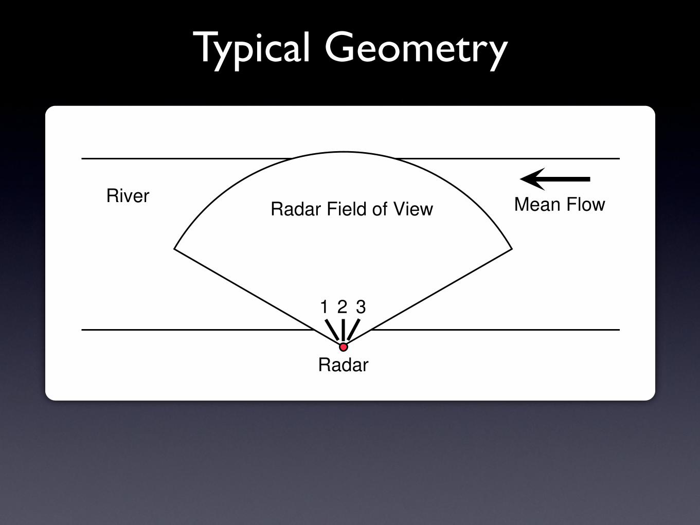
Typical Geometry

Radar Field of View Mean Flow

Radar

River

1 2 3

Newport Experiment

• CODAR student grant program

• Installed in September 2010 at Newport, Oregon

• Channel connecting Yaquina Bay to Pacific Ocean

• Tidal flow between parallel jetties

Experiment Location

Radial Vectors2010-12-07-13:00 UTC

Velocity Vector Estimation

• From a single site, find along- and cross-channel components from least-squares fit to radials

• If 2 sites are available, find full vectors by combining radial measurements from both sites

• From a single site, use Normal Modes Analysis of radial measurements to infer full vectors

• For arbitrary boundary, numerical solution required

• For rectangular boundary, closed-form solution possible

• Useful for dynamic flow conditions like tidal reversals

Normal Modes Analysis

• Assume water incompressible

• Express horizontal flow in terms of velocity potentials and stream func-

tions

• Boundary conditions

– Zero normal flow at banks

– No impedance to tangential flow at banks

– Periodic boundary at ends of analysis region

• Horizontal surface velocity vector−→U

−→U = ∇× [z(−Ψ) +∇× (zΦ)]

where z is the vertical unit vector, Ψ is the stream function, and Φ is

the velocity potential

• Allow up to 20 modes across river, only 2 along river

• Closed-form solutions in terms of sines and cosines

Homogeneous Equations• Stream function satisfying Dirichlet condition at bank

∇2ψn + νnψn = 0, where ψn|Γ = 0�uD

n , vDn

�=

�−∂ψn

∂y,

∂ψn

∂x

�

where ψn is the n-th eigenfunction of the stream function Ψ, νn is thecorresponding n-th eigenvalue and uD

n and vDn are the velocity compo-

nents in the x and y directions, respectively.

• Velocity function satisfying Neumann condition at bank

∇2φn + µnφn = 0, where (λ ·∇φn)��Γ

=∂φn

∂λ

��Γ

= 0

[uNn , vN

n ] =

�∂φn

∂x,

∂φn

∂y

�

where φn is the n-th eigenfunction of the velocity potential Φ, µn is thecorresponding n-th eigenvalue and λ is the direction perpendicular tothe boundary.

Normal Modes SolutionsVelocity potential modes with a periodic boundary at x = ±L/2 and bank at y = ±W/2

φn(x, y) =

cos(j2πx/L) cos(mπy/W )for j = 0,1,2,3, . . . ; m = 0,2,4,6, . . .

cos(j2πx/L) sin(mπy/W )for j = 0,1,2,3, . . . ; m = 1,3,5,7, . . .

sin(j2πx/L) cos(mπy/W )for j = 0,1,2,3, . . . ; m = 0,2,4,6, . . .

sin(j2πx/L) sin(mπy/W )for j = 0,1,2,3, . . . ; m = 1,3,5,7, . . .

Corresponding stream modes

ψn(x, y) =

cos(j2πx/L) cos(mπy/W )for j = 0,1,2,3, . . . ; m = 1,3,5,7, . . .

cos(j2πx/L) sin(mπy/W )for j = 0,1,2,3, . . . ; m = 0,2,4,6, . . .

sin(j2πx/L) cos(mπy/W )for j = 0,1,2,3, . . . ; m = 1,3,5,7, . . .

sin(j2πx/L) sin(mπy/W )for j = 0,1,2,3, . . . ; m = 0,2,4,6, . . .

Velocity Mode Examples 1

IfBdoPlotModes, BlockB8n, x0, y0, L, W<, L = x2 - x1; W = y2 - y1; x0 =x1 + x2

2; y0 =

y1 + y2

2;

For@n = 1, n § Length@uPhiD, n++, title = "n = " <> ToString@nD; title = modeIDPnT;plt = HVectorPlot@8uPhiPnT, vPhiPnT<, 8x, x1, x2<, 8y, y1, y2<, Frame Ø True,

PlotLabel Ø title, AspectRatio Ø Automatic, DisplayFunction Ø IdentityDL;Print@Show@plt, Graphics@8RGBColor@1, 0, 0D, Disk@80, 0<, 82, 2<D<D,

PlotRange Ø 88x1 - 10 - 0.01`, x2 + 10<, 8yp1, yp2<<,

ImageSize Ø modesPlotWidth, DisplayFunction Ø $DisplayFunctionDDD;F;F;

-400 -200 0 200 4000

50

100

150

200

250

300

35081, 0, -1, Null, Null<

-400 -200 0 200 4000

50

100

150

200

250

300

35082, 0, 0, Null, Null<

-400 -200 0 200 4000

50

100

150

200

250

300

35083, 0, 1, Null, Null<

-400 -200 0 200 4000

50

100

150

200

250

300

35084, 1, -1, Null, Null<

-400 -200 0 200 4000

50

100

150

200

250

300

35085, 1, 0, Null, Null<

-400 -200 0 200 4000

50

100

150

200

250

300

35086, 1, 1, Null, Null<

-400 -200 0 200 4000

50

100

150

200

250

300

35087, 2, -1, Null, Null<

2 FitModes6-ModePlots.nb

j = 1m = 0

j = 1m = 1

-400 -200 0 200 4000

50

100

150

200

250

300

35084, 1, -1, Null, Null<

-400 -200 0 200 4000

50

100

150

200

250

300

35085, 1, 0, Null, Null<

-400 -200 0 200 4000

50

100

150

200

250

300

35086, 1, 1, Null, Null<

-400 -200 0 200 4000

50

100

150

200

250

300

35087, 2, -1, Null, Null<

2 FitModes6-ModePlots.nb

-400 -200 0 200 4000

50

100

150

200

250

300

35088, 2, 0, Null, Null<

-400 -200 0 200 4000

50

100

150

200

250

300

35089, 2, 1, Null, Null<

-400 -200 0 200 4000

50

100

150

200

250

300

350810, 3, -1, Null, Null<

-400 -200 0 200 4000

50

100

150

200

250

300

350811, 3, 0, Null, Null<

FitModes6-ModePlots.nb 3


j = 0m = 1

j = 0m = 2


IfBdoPlotModes,

BlockB8n, x0, y0, L, W<, L = x2 - x1; W = y2 - y1; x0 =x1 + x2

2; y0 =

y1 + y2

2; For@n = 1,

n § Length@uPsiD, n++, title = "n = " <> ToString@nD; title = modeIDPLength@uPhiD + nT;plt = HVectorPlot@8uPsiPnT, vPsiPnT<, 8x, x1, x2<, 8y, y1, y2<, Frame Ø True,




-400 -200 0 200 4000

50

100

150

200

250

300

350864, Null, Null, 1, 0<

-400 -200 0 200 4000

50

100

150

200

250

300

350865, Null, Null, 2, 0<


IfBdoPlotModes,

BlockB8n, x0, y0, L, W<, L = x2 - x1; W = y2 - y1; x0 =x1 + x2

2; y0 =

y1 + y2

2; For@n = 1,

n § Length@uPsiD, n++, title = "n = " <> ToString@nD; title = modeIDPLength@uPhiD + nT;plt = HVectorPlot@8uPsiPnT, vPsiPnT<, 8x, x1, x2<, 8y, y1, y2<, Frame Ø True,




-400 -200 0 200 4000

50

100

150

200

250

300

350864, Null, Null, 1, 0<

-400 -200 0 200 4000

50

100

150

200

250

300

350865, Null, Null, 2, 0<


j = 0m = 1

j = 0m = 2

Mode Coefficients Determination

• Evaluate model in terms of unknown mode coefficients at each point where radar data are available

• At each point, equate sum of radial components of model to radial radar measurement

• Repeat over all available radar measurements

• Solve overdetermined set of equations for mode coefficients (~5000 equations in ~50 unknowns) using least-squares

• Allow up to 20 modes across river for along-river component (mmax), only 2 along river for both along- and cross-river components (jmax)

Streamline Examples

!200 !100 0 100 20050

100

150

200

250

300

x !m"

y!m"

NWPT_2010_12_07_0600

0.0

0.5

1.0

1.5

2.0

m#s

!200 !100 0 100 20050

100

150

200

250

300

x !m"

y!m"

NWPT_2010_12_07_0945

0.0

0.5

1.0

1.5

2.0

m#s

!200 !100 0 100 20050

100

150

200

250

300

x !m"

y!m"

NWPT_2010_12_07_1300

0.0

0.5

1.0

1.5

2.0

m#s

!200 !100 0 100 20050

100

150

200

250

300

x !m"

y!m"

NWPT_2010_12_07_1530

0.0

0.5

1.0

1.5

2.0

m#s

Mode Limits

u: jmax = 1, mmax = 5v: jmax = 0, mmax = 2

!200 !100 0 100 20050

100

150

200

250

300

x !m"

y!m"

NWPT_2010_12_07_1530

0.0

0.5

1.0

1.5

2.0

m#s

!200 !100 0 100 20050

100

150

200

250

300

x !m"

y!m"

NWPT_2010_12_07_1530

0.0

0.5

1.0

1.5

2.0

m#s u: jmax = 1, mmax = 20

v: jmax = 0, mmax = 2

Lagrangian Particle Trajectories

• Compute velocity vectors at 5-minute intervals

• Seed study area with 100 particles randomly placed every 2 minutes

• Integrate particle velocity in 10-second steps

• Display 10 locations of particles with lighter color for older positions

• Movie covers 2.5 hours around a tidal reversal

Particle Trajectory Example

!200 !100 0 100 20050

100

150

200

250

300

350

x !m"

y!m"

2010!12!07 08:30:00 !0000

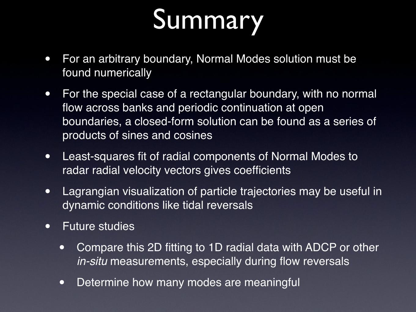
Summary• For an arbitrary boundary, Normal Modes solution must be

found numerically

• For the special case of a rectangular boundary, with no normal flow across banks and periodic continuation at open boundaries, a closed-form solution can be found as a series of products of sines and cosines

• Least-squares fit of radial components of Normal Modes to radar radial velocity vectors gives coefficients

• Lagrangian visualization of particle trajectories may be useful in dynamic conditions like tidal reversals

• Future studies

• Compare this 2D fitting to 1D radial data with ADCP or other in-situ measurements, especially during flow reversals

• Determine how many modes are meaningful

TU3.T10.2.pdf

Technology

TU3.T10.2.pdf