Trade Openness, Education and Growth
Parantap Basu1
Durham University
Keshab Bhattarai2
University of Hull
December 2008
Preliminary, Commets Welcome
1Department of Economics and Finance, Durham University, 23/26 Old Elvet,
Durham DH1 3HY, UK. e-mail: [email protected] School, University of Hull, HU6 7RX, Hull, UK. email:
Abstract
A signi�cant positive relationship exists between the trade share and educational
spending to GDP implying that countries which are more open on the trade front
also spend more on education. An open economy endogenous growth model with
human capital is developed to understand this stylized fact. The model demon-
strates that countries with greater cognitive skill spends more on education, and
grow faster. These countries open up on the trade front to �nance import of
physical capital which becomes scarce due to the diversion of resources to educa-
tion. The model highlights the importance of the productivity of human capital
or cognitive skill as an important economic fundamental determining the comove-
ment between trade share and education share. The Variance decomposition of
the shocks also con�rm that cognitive skill is important.
JEL Classi�cation: F41, O11, O33, O41
Keywords: Growth, Openness, Human capital, Cognitive Skill
1 Introduction
A plethora of literature exists about the relationship between openness and
growth. Grossman and Helpman (1990) show how openness promotes inno-
vation and growth in an open economy. Barro (1991) Mankiw, Romer and
Weil (1992), Jogenson and Fraumeni (1992), Parente and Prescott (2002))
took closed economy endogenous growth model to study theoretically and
empirically the link between growth and education leaving the trade issue
aside. Earlier Manning (1982) had shown how an increase in the educational
activity could reduce the amount of factors available for production of goods
and services in the short run but actually expands the production possibility
set when the level of skill rises in the long run. The literature has grown
further in recent years. Cartiglia (1997) had shown how trade liberalization
in skill scarce country leads to a higher investment in human capital and
creates the pattern of comparative advantage on international trade. Using
a multisectoral general equilibrium model Kim and Kim (2000) �nd that
education enhances mobility of workers across industries by enhancing their
human capital and removes the poverty trap. In a study of skill based wage
di¤erentials in Taiwan, Chang (2003) used a dynamic general equilibrium
model to establish how the education and the international trade were im-
portant factors in determining these wage di¤erentials. Basu and Guariglia
(2007) point out that FDI can complement human capital and could be bene-
�cial for growth at the expense of greater inequality. Despite all these studies
less is known whether countries which are more open on the trade front also
invest more in human capital. This is the central question addressed in this
paper.
1
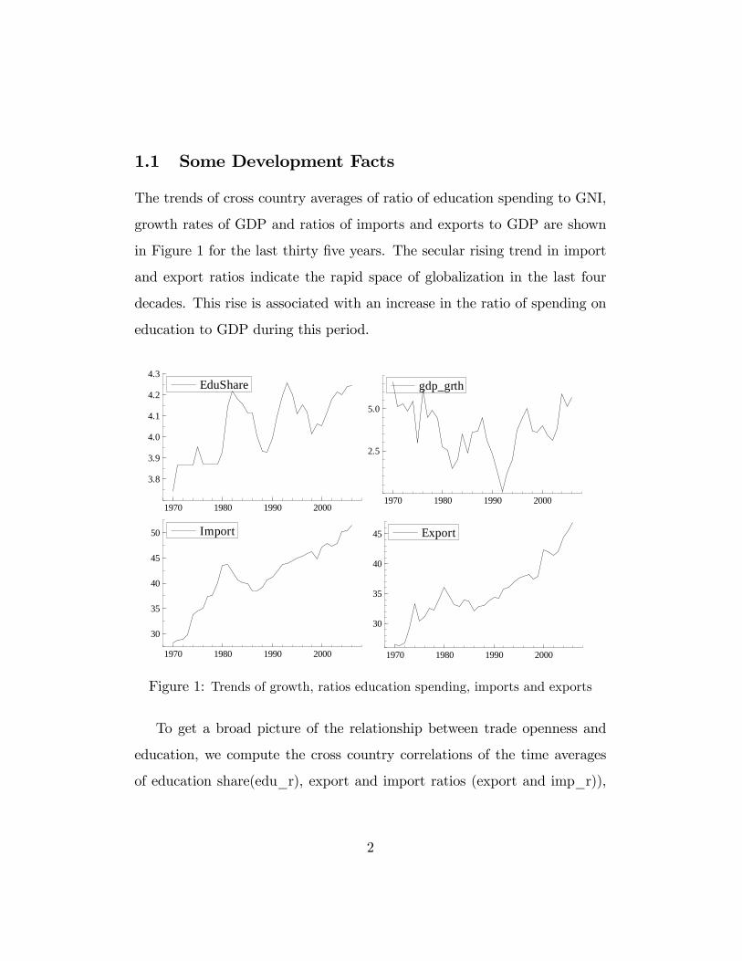
1.1 Some Development Facts
The trends of cross country averages of ratio of education spending to GNI,
growth rates of GDP and ratios of imports and exports to GDP are shown
in Figure 1 for the last thirty �ve years. The secular rising trend in import
and export ratios indicate the rapid space of globalization in the last four
decades. This rise is associated with an increase in the ratio of spending on
education to GDP during this period.
1970 1980 1990 2000
3.8
3.9
4.0
4.1
4.2
4.3EduShare
1970 1980 1990 2000
30
35
40
45 Export
1970 1980 1990 2000
30
35
40
45
50 Import
1970 1980 1990 2000
2.5
5.0
gdp_grth
Figure 1: Trends of growth, ratios education spending, imports and exports
To get a broad picture of the relationship between trade openness and
education, we compute the cross country correlations of the time averages
of education share(edu_r), export and import ratios (export and imp_r)),
2

growth rate (Growth) and total trade ratio (Trade_r).1
Table 1: Correlation coe¢ cients among ratios education spending, imports,
exports and growth
Edu_r Export Growth Imp_r Trade_r
Edu_r 1
Export_r 0.23 1
Growth -0.16 0.1687 1
Import_r 0.23 0.81 0.14 1
Trade_r 0.24 0.95 0.16 0.94 1
Correlations in Table 1 reveal the positive and signi�cant relation between
export share and education spending ratios implying that a country with a
higher spending on education has higher ratio of export to GDP. 2
1See http://www.esds.ac.uk/international/ and www.undp.org for detailed data source.
All the series came from the World Bank�s Development Indicator (WDI) database which
covers 206 countries.2Table 1 also re�ects a negative correlation between growth rates and education spend-
ing. This re�ects the fact that low income countries tend to grow faster than higher income
countries which makes the education share to correlate negatively with growth. To verify
this conjecture, we sort the data between low income and high income countries. For
low income countries, the correlation is -0.17 while for high income countries it is .002.
Also a panel regression of country growth rates on education shares after controlling for
country speci�c e¤ects provides a positive coe¢ cient which is not statistically signi�cant.
Given that the cross country growth shows tremendous disparity, locating only educa-
tion as a single explanatory variables may not be the way to determine education-growth
relationship.
3

The positive correlations between trade openness and education share are
reasonably robust with respect to �ner partitions of countries. Table 2 re-
ports the panel regression of export share and import shares on education
share after controlling for country speci�c e¤ects. The coe¢ cients of ed-
ucation share is statistically signi�cant at the 5% level in both regressions.
Panel ADF tests are run for each series to check for spurious correlations.
ADF test statistics are signi�cantly less than the critical value of -3.45.at 1
percent level of signi�cance indicating stationarity of each series. 3
Table 2: Panel Regressions of Export Ratio on Education Spending Ratio
Dep Variable: Export Ratio Coe¢ cient T-Value
Constant 10.61 4.33
Education ratio 2.58 4.54
R-square = 0.034; N =14; T=36 (1971-2006)
The aim of this paper is to understand this positive robust relationship
between trade openness and education. Our principal query is: why do coun-
tries which are more open on the trade front also invest more in education?
We answer this question in terms of a well articulated endogenous growth
3While running this panel regression, we controlled for country heterogeneity, and con-
ditional convergence. This is done by adding dummies for groups of countries, and adding
growth rate and level of GDP as regressors. Full details of these regressions are omitted
for brevity but available from the authors upon request.
4
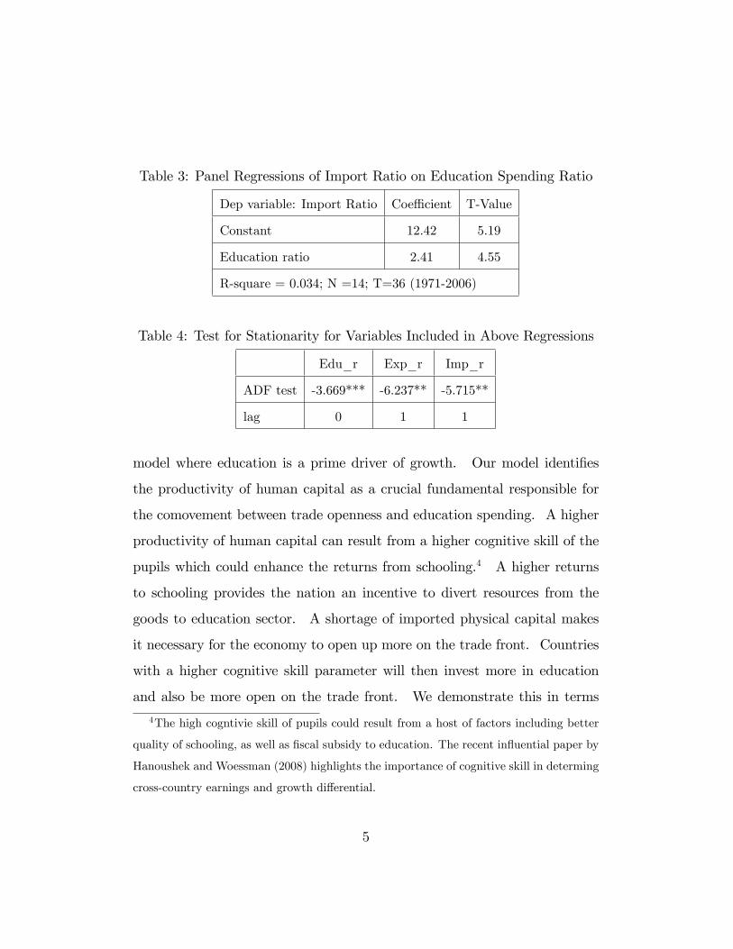
Table 3: Panel Regressions of Import Ratio on Education Spending Ratio
Dep variable: Import Ratio Coe¢ cient T-Value
Constant 12.42 5.19
Education ratio 2.41 4.55
R-square = 0.034; N =14; T=36 (1971-2006)
Table 4: Test for Stationarity for Variables Included in Above Regressions
Edu_r Exp_r Imp_r
ADF test -3.669*** -6.237** -5.715**
lag 0 1 1
model where education is a prime driver of growth. Our model identi�es
the productivity of human capital as a crucial fundamental responsible for
the comovement between trade openness and education spending. A higher
productivity of human capital can result from a higher cognitive skill of the
pupils which could enhance the returns from schooling.4 A higher returns
to schooling provides the nation an incentive to divert resources from the
goods to education sector. A shortage of imported physical capital makes
it necessary for the economy to open up more on the trade front. Countries
with a higher cognitive skill parameter will then invest more in education
and also be more open on the trade front. We demonstrate this in terms
4The high cogntivie skill of pupils could result from a host of factors including better
quality of schooling, as well as �scal subsidy to education. The recent in�uential paper by
Hanoushek and Woessman (2008) highlights the importance of cognitive skill in determing
cross-country earnings and growth di¤erential.
5
of an endogenous growth model in the tradition of Becker (1975) and Lucas
(1988) in an open economy context which is new in the literature.
The rest of the paper is organized as follows. The following section lays
out the model. Section 3 analyzes the long run properties of the model.
Section 4 performs short run analysis in terms of impulse responses and vari-
ance decompositions of shocks to goods and education productivity. Section
5 concludes.
2 The Model
The model is a small open economy adaptation of the Lucas-Uzawa (Lucas,
1988) model. There are two sectors, goods and education. The output in
the goods sector (yt) is produced with the help of imported physical capital
(kt) and home grown intangible or human capital (ht): Human capital is
augmented only with the aid of human capital and this activity is called
schooling. At any date t; a fraction lGt of human capital is allocated to the
goods sector and remaining fraction lHt is allocated to schooling. The human
capital evolves following the technology:
ht+1 = (1� �h)ht + AHtlHtht (1)
where AHt is the total factor productivity (TFP) in the education sector
at date t. This education TFP can be attributed to cognitive skills of pupils
in the home country. Quality of schooling and education subsidy could sig-
ni�cantly account for this variable. The introduction of this cognitive skill
6
variable is motivated by the recent work of Hanoushek andWoessman (2008).
Basu and Guariglia (2008) also use the same human capital investment tech-
nology to understand the e¤ect education on the pace of industrialization.
Final goods (yt) are produced with the help of human and physical capital
via the Cobb-Douglas production technology:
yt = AGtkt�(lGtht)
1�� (2)
where AGt is the the date t total factor productivity (TFP) in the goods
sector. We assume the following stationary stochastic processes for these
two TFP shocks around the steady state:
AGt ��AG = �G(AGt�1 �
�AG) + �
Gt (3)
AHt ��AH = �G(AHt�1 �
�AH) + �
Ht (4)
where�AGand
�AH as the steady state TFP of the goods and education
sectors. �G and �H are positive fractions and �Gt and �
Ht are white noises.
The goods are used for consumption (ct) and export (xt). The home
country faces a �xed price pk for investment goods (ikt ) . It �nances this
physical investment by a combination of export and foreign borrowing (bt)
at a �xed world interest rate, r�.
The resource constraint facing the country is:
ct + xt = yt (5)
7

xt + bt+1 = (1 + r�)bt + p
kikt (6)
ikt = kt+1 � (1� �k)kt (7)
The home country faces a borrowing constraint. The amount that it
can borrow in the international market is constrained by the current capital
stock which means:
bt � kt (8)
The timeline is as follows. At date t, the state of the economy is charac-
terized by kt, ht and bt. The home country after realizing the TFP shocks,
�Gt ; �Ht , makes decisions about goods production (yt), schooling (lHt), ex-
ports (xt); external borrowing (bt+1) and consumption (ct) which maximizes
the following expected utility functional.
E0
1Xt=0
�tU(ct)
subject to (2) through (8).
The lagrange at date t is:
Lt = Et1Ps=0
�sU(ct+s)+1Ps=0
�t+s[AGt+sk�t+s(lGt+sht+s)
1���ct+s�pkfkt+s+1�
(1� �k)kt+sg � (1 + r�)bt+s + bt+s+1]
+1Ps=0
�t+s[(1��h)ht+s+AHt+sf(1�lGt)ht+sg�ht+s+1]+1Ps=0
!t+s(kt+s�bt+s)
8

where �t; �t; !t are lagrange multiplier associated with the �ow budget
constraint (5), human capital technology, (1) and the borrowing constraint
(8).
First order conditions are:
ct : �tU 0(ct) = �t (9)
kt+1 : �tpk�Et!t+1 = Et�t+1fAGt+1�k��1t+1 (lGt+1ht+1g1��+(1� �k)pkg (10)
ht+1 : �t = Et�t+1f1� �h + AHt+1(1� lGt+1)g (11)
+Et�t+1fAGt+1(1� �)k�t+1h��t+1l1��Gt+1
lGt : �t(1� �)AGtl��Gt k�t ht1�� � �tAHht = 0 (12)
bt+1 : �t = Et(1 + r�)�t+1 + Et!t+1 (13)
3 Balanced Growth Properties
Hereafter we specialize to a logarithmic utility function, U(ct) to analyze the
long run and short run properties of the model. We also assume that the
borrowing constraint (8) binds. In the absence of any shock to technology,
9
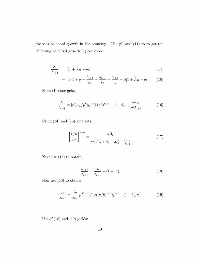
there is balanced growth in the economy. Use (9) and (11) to to get the
following balanced growth (g) equation:
�t�t+1
= [1 +�AH � �h] (14)
= > 1 + g =ht+1ht
=kt+1kt
=ct+1ct
= �[1 +�AH � �h] (15)
From (10) one gets:
�t�t+1
= [�(�AG=p
k)l1��G (k=h)��1 + 1� �k] +!t+1pk�t+1
(16)
Using (14) and (16), one gets:
�k=h
lG
�1��=
��AG
pk(�AH + �k � �h)� !t+1
�t+1
(17)
Next use (13) to obtain:
!t+1�t+1
=�t�t+1
� (1 + r�) (18)
Now use (10) to obtain
!t+1�t+1
=�t�t+1
pK � [�AG�(k=h)
��1l1��G + (1� �k)pk] (19)
Use of (18) and (19) yields:
10
�t�t+1
=1 + r� �
�AG�(k=h)
��1l1��G � (1� �k)pk1� pk =
1� pk + r� ��AG�(k=h)
��1l1��G + �kpk
1� pk(20)
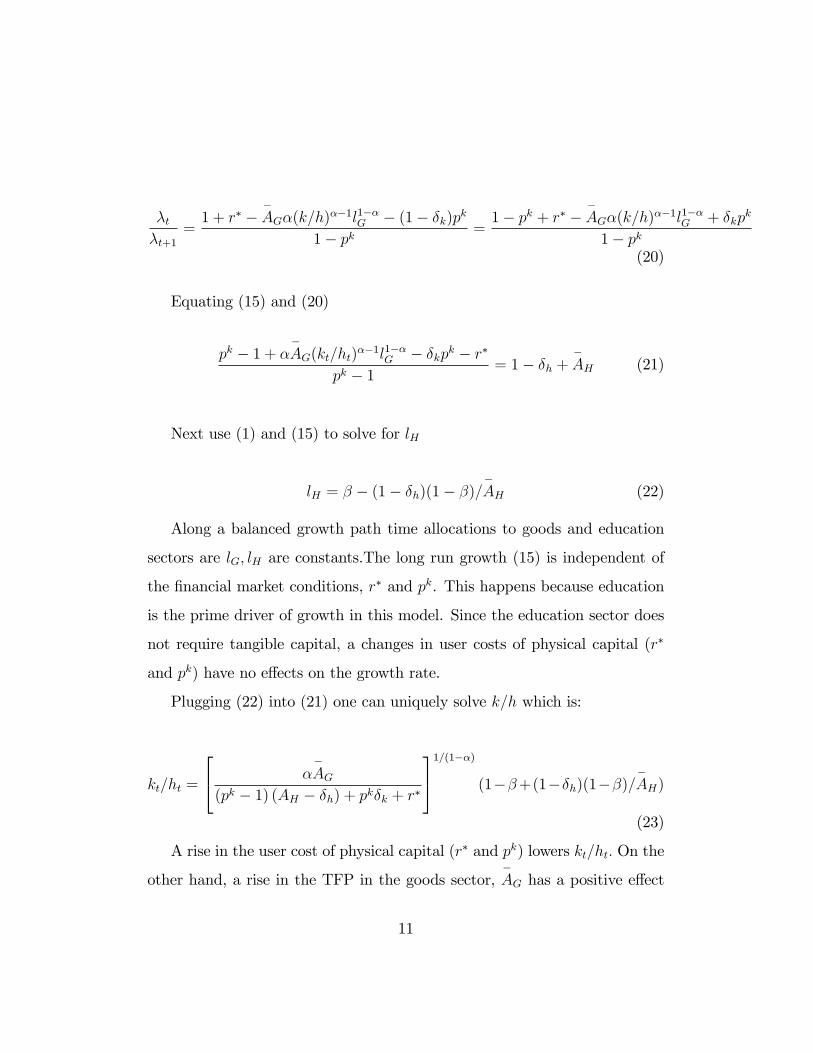
Equating (15) and (20)
pk � 1 + ��AG(kt=ht)
��1l1��G � �kpk � r�pk � 1 = 1� �h +
�AH (21)
Next use (1) and (15) to solve for lH
lH = � � (1� �h)(1� �)=�AH (22)
Along a balanced growth path time allocations to goods and education
sectors are lG; lH are constants.The long run growth (15) is independent of
the �nancial market conditions, r� and pk. This happens because education
is the prime driver of growth in this model. Since the education sector does
not require tangible capital, a changes in user costs of physical capital (r�
and pk) have no e¤ects on the growth rate.
Plugging (22) into (21) one can uniquely solve k=h which is:
kt=ht =
24 ��AG
(pk � 1) (AH � �h) + pk�k + r�
351=(1��) (1��+(1��h)(1��)=�AH)(23)
A rise in the user cost of physical capital (r� and pk) lowers kt=ht: On the
other hand, a rise in the TFP in the goods sector,�AG has a positive e¤ect
11
on kt=ht to keep the marginal product of physical capital constant because
the balanced growth rate (15) is independent of�AG:
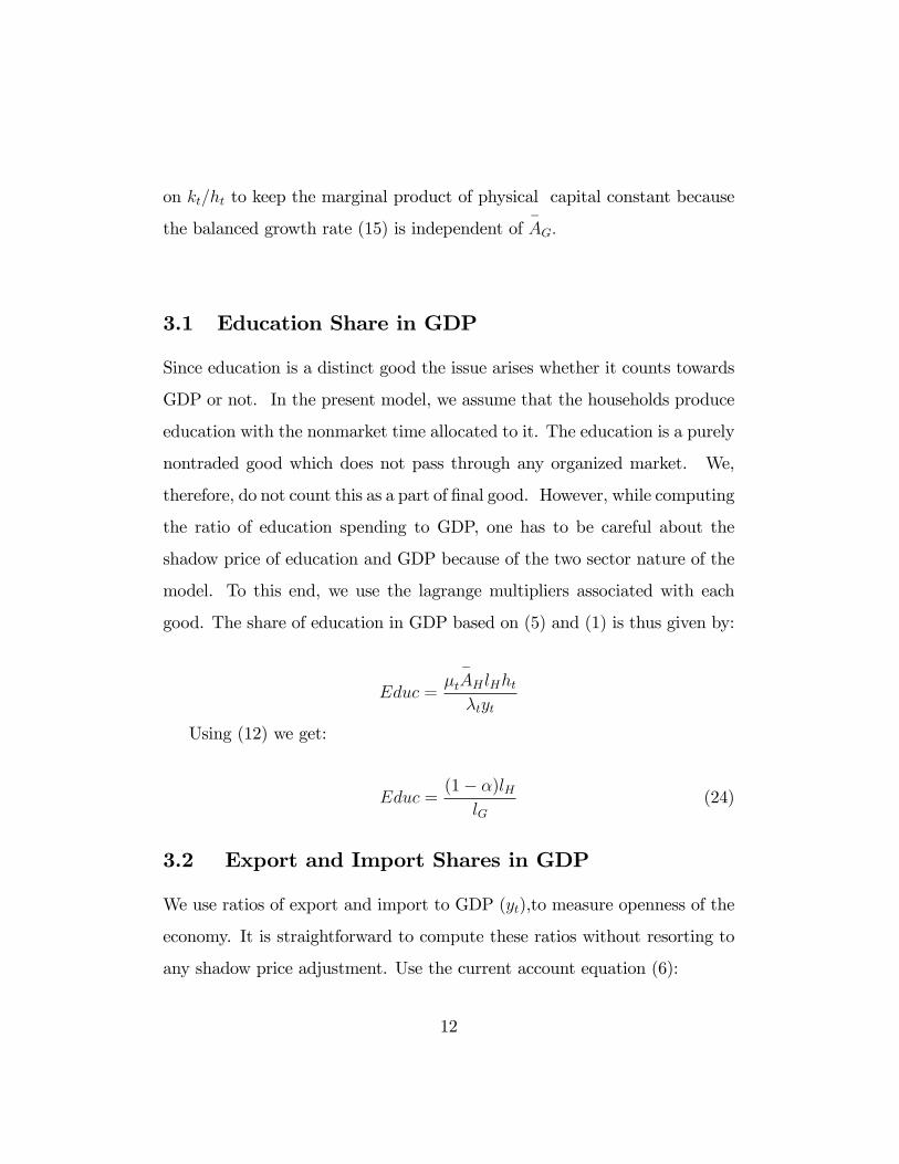
3.1 Education Share in GDP
Since education is a distinct good the issue arises whether it counts towards
GDP or not. In the present model, we assume that the households produce
education with the nonmarket time allocated to it. The education is a purely
nontraded good which does not pass through any organized market. We,
therefore, do not count this as a part of �nal good. However, while computing
the ratio of education spending to GDP, one has to be careful about the
shadow price of education and GDP because of the two sector nature of the
model. To this end, we use the lagrange multipliers associated with each
good. The share of education in GDP based on (5) and (1) is thus given by:
Educ =�t�AH lHht�tyt
Using (12) we get:
Educ =(1� �)lH
lG(24)
3.2 Export and Import Shares in GDP
We use ratios of export and import to GDP (yt),to measure openness of the
economy. It is straightforward to compute these ratios without resorting to
any shadow price adjustment. Use the current account equation (6):
12

xt + kt+1 = (1 + r�)kt + p
k[kt+1 � (1� �k)kt]
Divide through by kt and using the balanced growth rate (15) to get
xtyt=��(1� �h + AH)(pk � 1) + �(1 + r�)� �(1� �k)pk
MPK(25)
where the denominator is basically the marginal product of capital (MPK)
given as follows:
MPK = (pk � 1)AH + pk(�k � �h) + �h + r� (26)
Next de�ne the import share in GDP as:
mt
yt=pk(kt+1 � (1� �k)kt)
yt(27)
which after using the balanced growth rate (15) and the aggregate pro-
duction function reduces to:
mt
yt=�pkf�(1 +
�AH � �h)� (1� �k)gMPK
(28)
3.3 Baseline Calibration
This model is de�ned in terms of eight parameters,�AG ,
�AH , pk ,r�; �; �; �h; �k
which describe the preferences, technology and accumulation processes in the
economy. Our primary query is: what could contribute to a positive cross
country correlation between openness and education as seen in the data?.
13
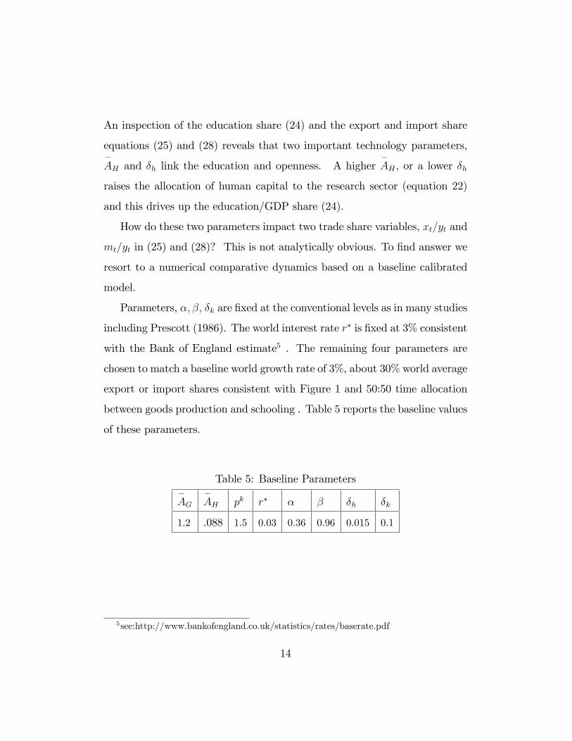
An inspection of the education share (24) and the export and import share
equations (25) and (28) reveals that two important technology parameters,�AH and �h link the education and openness. A higher
�AH ; or a lower �h
raises the allocation of human capital to the research sector (equation 22)
and this drives up the education/GDP share (24).
How do these two parameters impact two trade share variables, xt=yt and
mt=yt in (25) and (28)? This is not analytically obvious. To �nd answer we
resort to a numerical comparative dynamics based on a baseline calibrated
model.
Parameters, �; �; �k are �xed at the conventional levels as in many studies
including Prescott (1986). The world interest rate r� is �xed at 3% consistent
with the Bank of England estimate5 . The remaining four parameters are
chosen to match a baseline world growth rate of 3%, about 30% world average
export or import shares consistent with Figure 1 and 50:50 time allocation
between goods production and schooling . Table 5 reports the baseline values
of these parameters.
Table 5: Baseline Parameters�AG
�AH pk r� � � �h �k
1.2 .088 1.5 0.03 0.36 0.96 0.015 0.1
5see:http://www.bankofengland.co.uk/statistics/rates/baserate.pdf
14
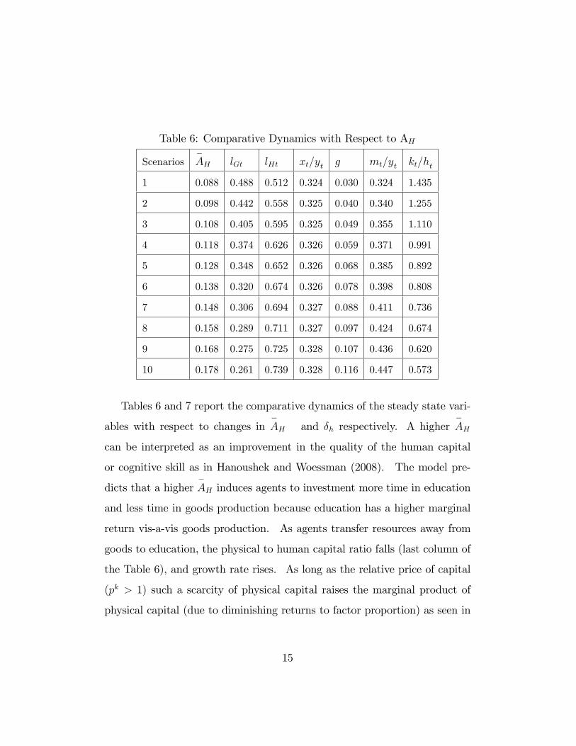
Table 6: Comparative Dynamics with Respect to AH
Scenarios�AH lGt lHt xt=yt g mt=yt kt=ht
1 0.088 0.488 0.512 0.324 0.030 0.324 1.435
2 0.098 0.442 0.558 0.325 0.040 0.340 1.255
3 0.108 0.405 0.595 0.325 0.049 0.355 1.110
4 0.118 0.374 0.626 0.326 0.059 0.371 0.991
5 0.128 0.348 0.652 0.326 0.068 0.385 0.892
6 0.138 0.320 0.674 0.326 0.078 0.398 0.808
7 0.148 0.306 0.694 0.327 0.088 0.411 0.736
8 0.158 0.289 0.711 0.327 0.097 0.424 0.674
9 0.168 0.275 0.725 0.328 0.107 0.436 0.620
10 0.178 0.261 0.739 0.328 0.116 0.447 0.573
Tables 6 and 7 report the comparative dynamics of the steady state vari-
ables with respect to changes in�AH and �h respectively. A higher
�AH
can be interpreted as an improvement in the quality of the human capital
or cognitive skill as in Hanoushek and Woessman (2008). The model pre-
dicts that a higher�AH induces agents to investment more time in education
and less time in goods production because education has a higher marginal
return vis-a-vis goods production. As agents transfer resources away from
goods to education, the physical to human capital ratio falls (last column of
the Table 6), and growth rate rises. As long as the relative price of capital
(pk > 1) such a scarcity of physical capital raises the marginal product of
physical capital (due to diminishing returns to factor proportion) as seen in
15

Table 7: Comparative Dynamics with Respect to dh
Scenarios �h lGt lHt xt=yt mt=yt g kt=ht
1 0.015 0.488 0.512 0.3243 0.3244 0.030 1.435
2 0.016 0.488 0.513 0.3243 0.3236 0.030 1.437
3 0.016 0.487 0.513 0.3243 0.3228 0.029 1.439
4 0.017 0.487 0.513 0.3242 0.3220 0.029 1.441
5 0.017 0.487 0.513 0.3242 0.3211 0.028 1.443
6 0.018 0.487 0.513 0.3242 0.3203 0.028 1.445
7 0.018 0.486 0.514 0.3242 0.3195 0.027 1.447
8 0.019 0.486 0.514 0.3241 0.3186 0.027 1.449
9 0.019 0.486 0.514 0.3241 0.3178 0.026 1.451
10 0.020 0.486 0.514 0.3241 0.3170 0.026 1.453
(26). Since the home country has the option to augment physical capital by
�nancing it through current account, it will take advantage of it by raising
its export and import share. Thus the country becomes more open on the
trade front. The bottomline is that as a consequence of higher�AH , the home
country invests more in education, its growth rises via the human capital
equation (1) and its trade share also increases. The e¤ect of a lower rate of
depreciation in �h is analogous to a higher�AHas can be read from Table 7
although its e¤ect is small compared to�AH .
16

4 Short Run Dynamics
Until now we only analyzed the steady states of the model. Such a steady
state analysis can be motivated by cross country comparison of various long
run averages such as average growth, trade share, education share. The
underlying assumption here is that each country is in di¤erent long run steady
states and the research question is what drives this cross country dispersion.
We identify TFP in each sector as a major fundamental for the cross country
dispersion of growth, education share and trade share. However, such a
long run analysis cannot re�ect how a country can respond to shocks to its
fundamentals. Analysis of this kind of within-country response to shocks
necessitates a short run analysis.
The short run system is given by equations (29) to (36) as following(The
appendix shows the derivation of these equations).
kt+1ht+1
=pk (1� �k) ktht + AGt(
ktht)�l1��Gt � ct
ht� (1 + r�) kt
ht
(pk � 1) f1� �h + AHt(1� lGt)g(29)
1 = mt+1:�AGt+1
�kt+1ht+1
���1l1��Gt+1 + (1� �k)pk � 1� r�
pk � 1 (30)
AGtAht
:l��Gt :(ktht)� =
mt+1
�AGt+1Aht+1
:l��Gt+1:(kt+1ht+1
)� f1� �h + AHt+1(1� lGt+1)g+ AGt+1�kt+1ht+1
��l1��Gt+1
�(31)
where mt+1 is the discount factor given by
17

mt+1 =�(ct=ht)
(ct+1=ht+1)
1
(AHt+1(1� lGt+1) + 1� �h)(32)
Export and import share equations are given by:
xtyt
= [1 + r� � pk(1� �k)](kt=yt) (33)
+(pk � 1)(kt+1=yt+1)(AGt+1=AGt)�kt+1=ht+1kt=ht
��f1� �h + AHtlhtg:
�lGt+1lGt
�1��
mt
yt= pk
"kt+1yt+1
:AGt+1AGt
:
�kt+1=ht+1kt=ht
���lGt+1lGt
�1��f1� �h + AHtlhtg � (1� �k):
ktyt
#(34)
The ratio of current account to GDP is de�ned as:
catyt=xtyt� mt
yt(35)
The physical capital:output ratio is given by the production function (2)
as:
ktyt= A�1Gt (kt=ht)
1��l��1Gt (36)
The education share equation is given by:
Educt =(1� �)lHt
lGt(37)
Finally the gorwth rate of output is given by:
18
yt+1yt
=AGt+1AGt
:
�AGt+1AGt
� �kt+1=ht+1kt=ht
��fAHtlHt + 1� �hg:
�lGt+1lGt
�1��(38)
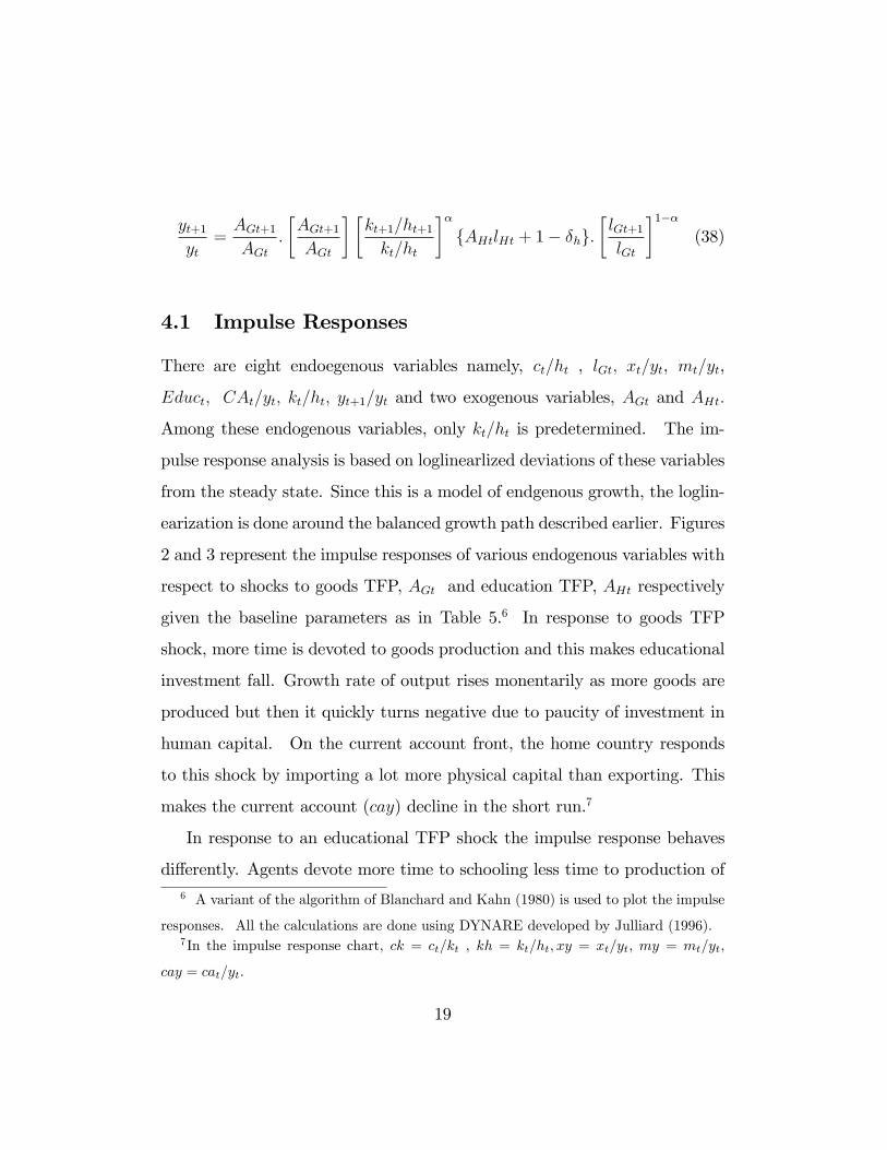
4.1 Impulse Responses
There are eight endoegenous variables namely, ct=ht , lGt; xt=yt, mt=yt,
Educt; CAt=yt; kt=ht; yt+1=yt and two exogenous variables, AGt and AHt:
Among these endogenous variables, only kt=ht is predetermined. The im-
pulse response analysis is based on loglinearlized deviations of these variables
from the steady state. Since this is a model of endgenous growth, the loglin-
earization is done around the balanced growth path described earlier. Figures
2 and 3 represent the impulse responses of various endogenous variables with
respect to shocks to goods TFP, AGt and education TFP, AHt respectively
given the baseline parameters as in Table 5.6 In response to goods TFP
shock, more time is devoted to goods production and this makes educational
investment fall. Growth rate of output rises monentarily as more goods are
produced but then it quickly turns negative due to paucity of investment in
human capital. On the current account front, the home country responds
to this shock by importing a lot more physical capital than exporting. This
makes the current account (cay) decline in the short run.7
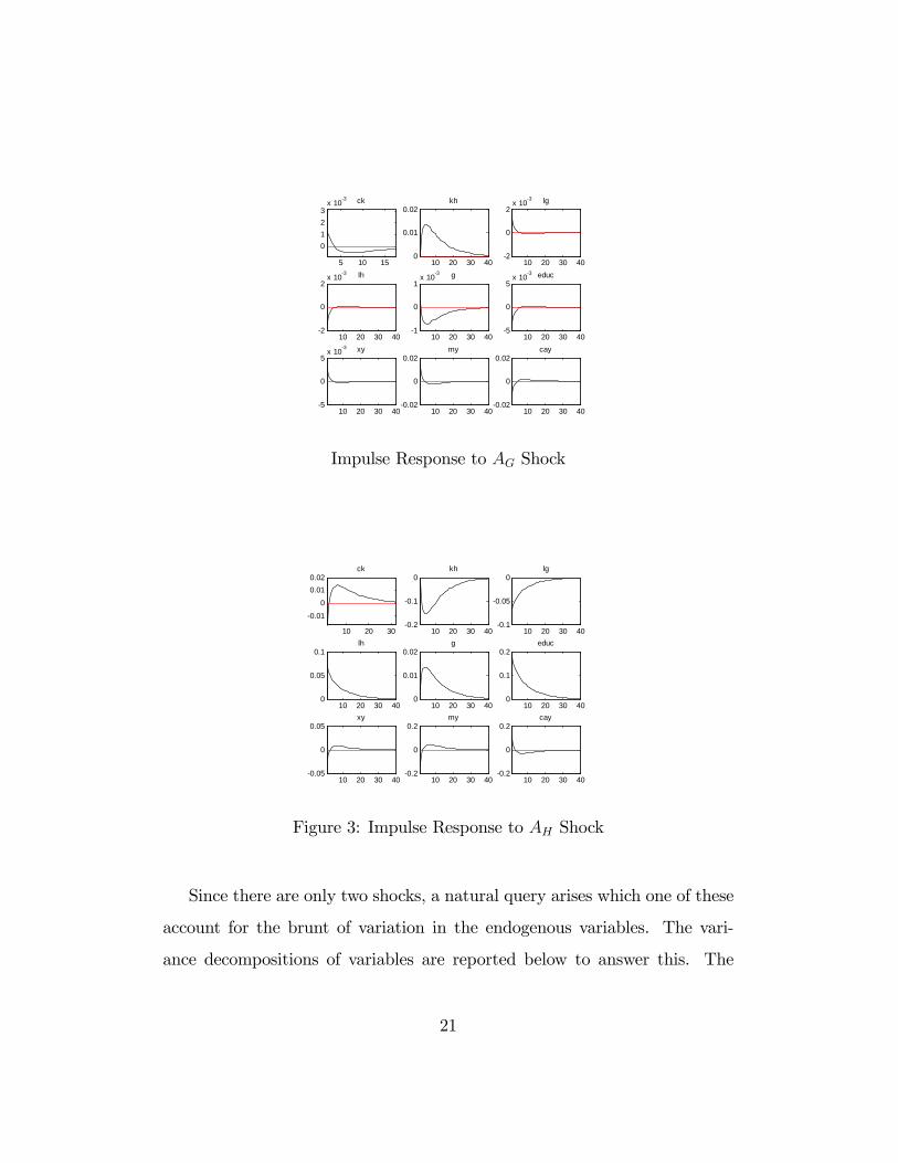
In response to an educational TFP shock the impulse response behaves
di¤erently. Agents devote more time to schooling less time to production of6 A variant of the algorithm of Blanchard and Kahn (1980) is used to plot the impulse
responses. All the calculations are done using DYNARE developed by Julliard (1996).7In the impulse response chart, ck = ct=kt , kh = kt=ht; xy = xt=yt; my = mt=yt,
cay = cat=yt:
19
�nal goods. Growth rate of output rises due to transfer of resources from
goods to education sector and then it picks up as more schooling increases the
human capital base. Both export and import shares fall although the latter
falls more than the former making the current account rise. At a later stage,
the nation starts allocating more resources to the goods sector which makes
import and export share rise. The current account shows greater volatility
in response to this shock.
Note the contrast between long run and short run e¤ects of AG: First, In
the long run scenario, a change in AG has neutral e¤ects on growth, education
and trade shares while this is not the case in the short run. A shock to goods
sector productivity has important e¤ects on time allocation to schooling and
hence growth and openness.
Second, the short run response of shocks to cognitive skill is remarkably
di¤erent from what we see in the long run. While in the long run, a higher
AH results in a higher trade share, a temporary positive shock to AH makes
the home country cut back in exports and imports to allow for growth in the
education sector. 8
8The short run correlation between trade share and education is negative while cross
country data suggets that it is positive. Note that the cross country correlations referes to
the long run comparision of countries which di¤er in terms of long run average TFP. This
basically means between-country variation in trade shares and education shares. The
short run analysis can be interpreted as within-country response of a transitory shock to
productivity.
20
5 10 15
0123
x 103 ck
10 20 30 400
0.01
0.02kh
10 20 30 402
0
2x 10³ lg
10 20 30 402
0
2x 10
3 lh
10 20 30 401
0
1x 10
3 g
10 20 30 405
0
5x 10
3 educ
10 20 30 405
0
5x 10³ xy
10 20 30 400.02
0
0.02my
10 20 30 400.02
0
0.02cay
Impulse Response to AG Shock
10 20 30
0.01
0
0.010.02
ck
10 20 30 400.2
0.1
0kh
10 20 30 400.1
0.05
0lg
10 20 30 400
0.05
0.1lh
10 20 30 400
0.01
0.02g
10 20 30 400
0.1
0.2educ
10 20 30 400.05
0
0.05xy
10 20 30 400.2
0
0.2my
10 20 30 400.2
0
0.2cay
Figure 3: Impulse Response to AH Shock
Since there are only two shocks, a natural query arises which one of these
account for the brunt of variation in the endogenous variables. The vari-
ance decompositions of variables are reported below to answer this. The
21
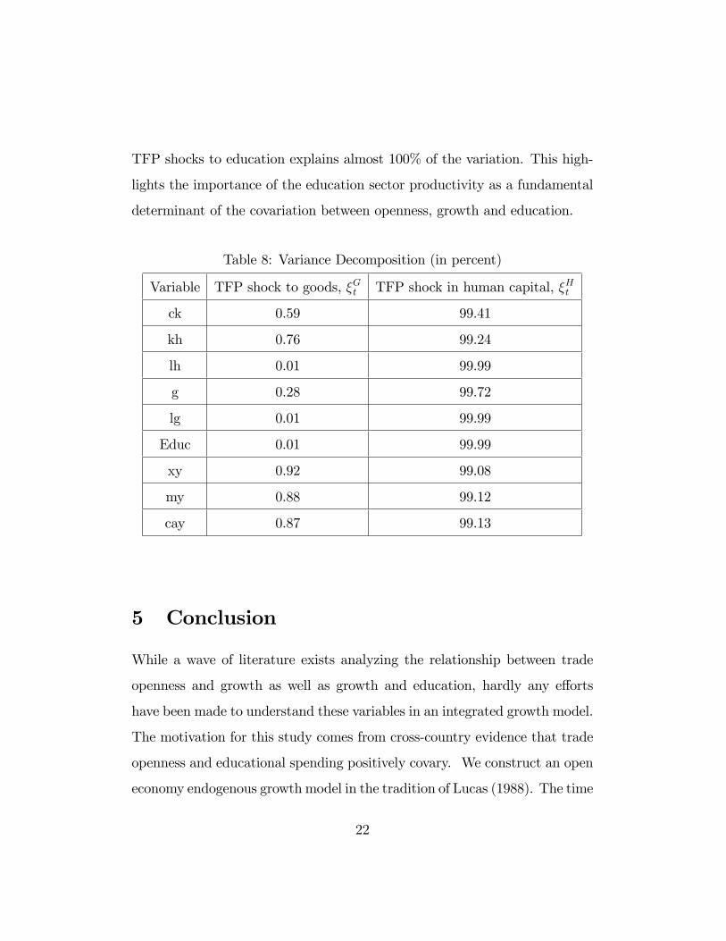
TFP shocks to education explains almost 100% of the variation. This high-
lights the importance of the education sector productivity as a fundamental
determinant of the covariation between openness, growth and education.
Table 8: Variance Decomposition (in percent)
Variable TFP shock to goods, �Gt TFP shock in human capital, �Ht
ck 0.59 99.41
kh 0.76 99.24
lh 0.01 99.99
g 0.28 99.72
lg 0.01 99.99
Educ 0.01 99.99
xy 0.92 99.08
my 0.88 99.12
cay 0.87 99.13
5 Conclusion
While a wave of literature exists analyzing the relationship between trade
openness and growth as well as growth and education, hardly any e¤orts
have been made to understand these variables in an integrated growth model.
The motivation for this study comes from cross-country evidence that trade
openness and educational spending positively covary. We construct an open
economy endogenous growth model in the tradition of Lucas (1988). The time
22
allocation between goods production and schooling is an essential ingredient
of human capital growth. Our model identi�es the productivity of human
capital as a crucial fundamental causing this comovement between education
and trade openness. This fundamental can be interpreted as cognitive skill
along the lines of a recent literature which pinpoints cognitive skill as a critical
determinant of growth. While cognitive skill is an exogenous technology
variable in our model, future research can delve deeper into the underlying
reasons for the cross country di¤erences in cognitive skills.
References
[1] Barro R. J.(1991) Economic Growth in Cross Section of Countries, Quar-
terly Journal of Economics, May, 407-433.
[2] Basu P and A Guariglia (2008) Does low education delay structural
transformation, Southern Economic Journal, forthcoming.
[3] Becker G.S. (1975) Human Capital, Columbia University, New York.
[4] Blanchard, O and C.M. Kahn (1980), The Solution of Linear Di¤erence
Models under Rational Expectations, Econometrica 48, pp. 1305-1313.
[5] Cartiglia F. (1997) Credit constraints and human capital accumulation
in the open economy, Journal of International Economics, 43, 221:236.
[6] Chang H C (2003) International trade, productivity growth, education
and wage di¤erential: A case study of Taiwan, Journal of Applied Eco-
nomics, 6:1:25-48.
23
[7] Findlay R and H Kierzkowski (1983) International trade and human cap-
ital: A simple general equilibrium model, Journal of Political Economy,
91:6:957-978.
[8] Grossman G.M. and E. Helpman (1990) Comparative Advantage and
Long-Run Growth, American
Economic Review, 80:4:796-815
[9] Hanushek E A and L Woessmann (2008) The Role of Cognitive Skills in
Economic Development, Journal of Economic Literature, 46:3:607-668,
September.
[10] Jogenson DW and B. Fraumeni (1992) Investment in Education and US
Economic Growth, Scandinavian Journal of Economics 94:51-70, Sep-
tember.
[11] Juillard, M (1996), Dynare: A Program for the Resolution and Simula-
tion of Dynamic Models with Forward Variables through the Use of a
Relaxation Algorithm, CEPREMAP, Couverture Orange, 9602,
[12] Kim S J and Y J Kim (2000) Growth gains from trade and education,
Journal of International Economics, 50:519-545.
[13] Lucas R.E. (1988) On the Mechanics of Economic Development, Journal
of Monetary Economics, 22:1: 3-42.
[14] Mankiw N.G., D. Romer and D. N. Weil (1992) Contribution to the
Empirics of Economic Growth,Quarterly Journal of Economics, 107:407-
437, May.
24

[15] Manning R. (1982) Trade, Education and Growth: The Small-Country
Case, International Economic Review, 23:1:83-106.
[16] Owen A L (1999) International trade and the accumulation of human
capital, Southern Economic Journal, 66:1:61-81.
[17] Parente S.L. and E.C. Prescott (2002) Barriers to Riches, MIT Press.
[18] Prescott, E.C. (1986), Theory Ahead of Business Cycle Measurement,
Federal Reserve Bank of Minneapolis, Quarterly Review; Fall.
[19] Romer, Paul (1989) Endogenous Technological Change, Journal of Po-
litical Economy, 98:5: Pt. 2: S71-S102.
25

6 Appendix
Use (5), (6), (7), (8) with equality to get:
kt+1 =pk(1� �k)kt + AGtk�t (lGtht)1�� � ct � (1 + r�)kt
pk � 1 (39)
Dividing (39) by (1), one gets (29).
(30) can be obtained by combining (9),(10) and (13).
Use (11) and (12) to obtain (31).
The discount factor (32) is basically �ct=ct+1 . This can be rewritten as
�f(ct=ht)=(ct+1=ht+1)g(ht+1=ht)�1: After using (1), one gets the expression
for (32).
To obtain the export share equation (33) , use (6) and (8) to obtain:
xt = (1 + r�)kt + (p
k � 1)kt+1 � pk(1� �k)kt
Divide through by yt to obtain
xtyt= (1 + r� � pk(1� �k))
ktyt+ (pk � 1)(kt+1
yt+1)(yt+1yt)
Next use the production function (2) and the human capital equation (1)
to obtain (33).
To get (34), use (27)
mt
yt=pk(kt+1 � (1� �k)kt)
yt
which can be rewritten as:
26

mt
yt= pk(
kt+1yt+1
:yt+1yt
� (1� �k)ktyt)
which after using the production function (2) and the human capital
equation (1) yields the expression (34).
The expression for (36) directly follows from the production function (2).
The expression for (37) is the same as the steady state expression (24).
The expression for the growth rate in (38) follows from the use of the
production function (2) and the human capital equation (1).
27