1
Trade liberalization and SO2 emissions:
Firm -level evidence from China’s WTO entry
Lei Li (Nankai University, China), Andreas Löschel (Westfälische Wilhelms-Universität Münster, ZEW Mannheim, Germany, UIBE, China), Jiansuo Pei (UIBE, China), Bodo Sturm (HTWK Leipzig, ZEW Mannheim, Germany), and
Anqi Yu (UIBE, China)
Abstract: Is trade liberalization contributing to cleaner production amongst manufacturing
firms? Theoretical predictions and empirical evidences are mixed. This study utilizes China’s
dual trade regime and China’s WTO entry in 2001 to construct a unique micro dataset on
manufacturing firms for China for the period 2000-2007, and performs a
difference-in-difference estimation strategy to directly examine this issue. Specifically,
normal exporters that saw tariff changes during the same period form the treatment group;
while processing exporters that enjoy tariff-exemptions both pre- and post-WTO entry serve
as the control group. Results show that China’s WTO entry contributed to a lower SO2
emission intensity for normal exporting firms. We further examine the mechanism and show
that the productivity channel accounted for the observed pattern. Specifically, more efficient
normal exporters saw greater decline of SO2 emission intensity than average normal exporters.
This study contributes to a better understanding of the impact of trade on the environment,
especially in developing countries. It also complements the literature in terms of providing
China’s micro evidence on the impact of trade liberalization on firm’s environmental
performance.
Keywords: WTO; trade liberalization; dual trade regime; SO2 emission intensity; China
JEL codes: F18; Q53; Q56
Acknowledgements: We are very grateful to constructive comments and suggestions from seminar participants, in
particular from Kathrine von Graevenitz and Robert Germeshausen, at the ZEW – Leibniz
Centre for European Economic Research. Financial support by the National Natural Science
Foundation of China (No. 41675139; 72042003) and the German Federal Ministry of
Education and Research (INTEGRATE, FKZ: 01LP1928A) is gratefully acknowledged. The
authors are listed alphabetically by last name.

2
1. Introduction
The degradation of the environment in developing countries has been one of the most
challenging policy issues of recent times. The massive growth in world trade might be
the main source of this problem. On the one hand, there are theoretical and empirical
concerns that the developing world acts as a “pollution haven” for the developed
world (e.g., Copeland and Taylor, 2004; Kellenberg, 2009). In addition, empirical
evidence shows that trends of local pollution in developed countries are declining
strongly (e.g. WIOD 2013 & 2016). On the other hand, trade may lead to structural
changes, efficiency gains and technological improvements which could contribute to
less pollution in developing countries.
China is not only key to understanding whether trade is good or bad for the
environment in developing countries, it is also the most prominent example both in
terms of export growth and growth in sulfur dioxide (SO2) emissions,1 especially
after its accession to the World Trade Organization (WTO). From 2001 till 2007
(before the financial crisis in 2008/09), the trade volume soared from about half
trillion RMB (i.e., 51 million USD in 2001) to 1.8 trillion RMB in 2007; and during
the same period, SO2 emissions grew from 21.9Mt to 27.9Mt. China now is one of the
world’s biggest SO2 emitters and simultaneously plays an important and increasing
role in trade. Will this exacerbate the problem or bring improvements in SO2
pollution?
Answering this question is central to understanding the environmental effects of
trade liberalization. For instance, one strand of research argues that international trade
is not conducive to improvements in environmental quality or at best the effect is
ambiguous. Classical discussions date back to Leontief (1970). More recently, Cole et
al. (2006) used energy consumption as the main dependent variable (rather than
1 There are several reasons why a focus on SO2 is warranted. SO2 emissions are primarily industry-driven (rather than generated by transportation or household activity) and the corresponding negative effects are local (rather than trans-boundary or global). Furthermore, different abatement technologies exist. In fact, China ranks the first for total SO2 emissions in the world, and emitted 30.8Mt in 2010 (Klimont et al., 2013). The SO2 emission intensity (measured by SO2 emissions per unit of total output), however, gradually declined from 13.60t/million dollars in 1997 to 1.45t/million dollars in 2014 or respectively by about 12 percent per year (Source: WIOD 2013 & 2016; National Bulletin of Environmental Statistics of China, various years).

3
various pollutants) and found a positive correlation between the degree of trade
openness and per capita energy consumption. Recently, Shapiro and Walker (2018)
report a large role of technique effects and very small trade-induced composition
effects. In contrast, Cherniwchan (2017), who uses NAFTA as a policy shock to
examine the effects of trade liberalization and the pollution emitted by US
manufacturing plants, shows that ratification of NAFTA accounted for a substantial
decline of particulate matter and SO2 emissions from affected US manufacturing
plants. In other words, trade liberalization is found to be an important driving force
for reductions of pollution for manufacturing plants. In this vein, World Development
Report 2020, the flagship report by the World Bank, recognizes the ambiguous effects
of international trade on the environment (see Chapter 5).
To examine this problem, relying on aggregate data (either industry and/or region)
as a standard practice has provided robust empirical evidence on the differential
effects of trade liberalization across heterogeneous regions and sectors (see Dean and
Lovely, 2010).2 However, these studies do not offer much insight on the behavior of
individual polluters within each industry. In this paper, we move beyond the
relationship between trade and aggregate pollution levels and study the firms’
responses (in terms of pollution behavior, measured by emissions per unit of total
output) to China’s WTO entry, a trade shock that accounts for the increase in market
competition in China. Specifically, we focus on SO2 emissions, one of the main local
pollutants with severe negative effects for the environment and human health in China
(HEI, 2016).
This paper builds on a unique dataset to investigate the manufacturing firms’
environmental responses to trade liberalization. Specifically, we utilized data during
the period 2000-2007, and took China’s WTO entry in 2001 as a quasi-experimental
setting, to perform a difference-in-difference (DID) estimation. In this way, we are
able to directly examine the impact of trade liberalization on firms’ environmental
performance. To that end, we combined and merged three rich firm-level datasets for
2 They point out the heterogeneous performance of different firms, an important aspect that will be further considered in our study.

4
China, namely the National Bureau of Statistics’ annual survey of industrial
production (ASIP), which shows firm-level production information; the Chinese
environmental statistics database (CESD) obtained from the Ministry of Ecology and
Environment; and customs data provided by China Customs plus tariff data obtained
from WITS (World Integrated Trade Solution, developed and maintained by
UNCTAD and World Bank). A total of 13,641 manufacturing observations were
successfully matched. To the best of our knowledge, it is the first time that this unique
dataset has been constructed and used in this line of research.
The identification in this paper is made possible due to China’s dual trade regime.
In addition to the normal trade regime, there is a special treatment of processing trade.
Specifically, processing trade refers to a trade mode in which firms import raw
materials, or parts and components from other countries, combining with their own
land or labor resources, process them into final products and then export. In fact,
processing exports accounted for over half of China's total exports for the period
1996-2007 (see Yu, 2015; Dietzenbacher et al., 2012).
The tariff reduction after China joined the WTO has had different effects on the
enterprises engaged in processing trade and normal trade (in several aspects, e.g.
declining input costs). Theoretically speaking, for the enterprises participating in
processing trade, the impact of trade liberalization on their environmental
performances should be relatively small, as processing trade enjoys tax-free treatment
both before and after the trade shock (i.e., these firms were not directly affected by the
shock). While the firms engaged in normal trade did not enjoy a preferential tariff
before China's accession to the WTO, yet saw an import tariff decline after China's
accession to the WTO (i.e., these firms were directly affected by the shock). Therefore,
it is expected that the impact of trade liberalization on pollutant discharges of normal
trade enterprises is greater compared to processing trade enterprises.
Using processing exporters that enjoy tariff-exemptions both pre- and post-WTO
entry as the control group and normal exporters that saw tariff changes during the
same period as the treatment group, our empirical findings can be summarized as

5
follows. China’s WTO entry contributed to lower SO2 emission intensity for normal
exporters. Specifically, compared with processing exporters that are not directly
affected by trade liberalization, SO2 emission intensity of normal exporters is
statistically significantly reduced by roughly 6% after China's accession to WTO.
Hence, China’s WTO entry accounted for a lower SO2 emission intensity for normal
exporters, which is in line with previous evidence reported for developed economies
(see Cherniwchan, 2017). In order to provide supportive evidence for our approach,
we conducted a falsification test, in which hybrid exporters (performing both
processing and normal exports) replaced the pure normal exporters. As expected, the
impact of China's accession to the WTO on the SO2 emission intensity of hybrid
exporters is no longer statistically significant. We also study possible confounding
effects of two policy reforms, i.e. the reform of state-owned enterprises and the
relaxation of regulations on the entry of foreign invested enterprises. China's
accession to the WTO still has a significantly negative impact on the SO2 emissions
intensity. We show that these effects vary across ownership in different regions.
In theory, there are several potential mechanisms which may be accountable for
this pattern, our focus here however is on the ones described by Melitz (2003) model
with heterogeneous firms. China's accession to the WTO might impact enterprises
engaged in normal export via different channels: First, through the productivity
channel, i.e. lower input costs (due to lower import tariffs) result in higher
productivity, and productivity is negatively related to firms’ emission intensity
(Forslid et al., 2018). Second, through the dynamics of firm entry and exit, i.e. the
reallocation of market shares, trade openness increases local competition and forces
the least productive (also the most polluting) firms to exit the exporting market, and
non-exporters to scale down their production. Previous studies have shown that more
productive firms are cleaner for a given productivity level since they find it profitable
to make larger fixed investments in clean technology (e.g., due to more stringent
environmental regulations) (see e.g., Forslid et al., 2018). We observe that these
properties are consistent with Chinese manufacturing survey data, which contains rich

6
information at the firm level. Indeed, our results show that especially more productive
normal exporters became cleaner (with lower SO2 emissions per output) after China's
accession to the WTO.
We make three main contributions to the literature: first, relative to other recent
micro data work on environmental effects of trade liberalization in developed
countries, we constructed a unique dataset for China from the merger of three rich
firm-level datasets. It allows us to conduct in-depth study for the environmental
performance (i.e., SO2 emission intensity) of Chinese firms due to trade shocks.
Second, we study the impact of trade liberalization on the environment at granular
firm level, taking advantage of China’s dual trade regime (processing vs. normal
exports). Third, we make use of China's accession to the WTO in 2001 as a
semi-natural policy shock to perform a DID estimation strategy that directly tackles
the potential endogeneity problem (i.e., the simultaneity issue),3 which is key in order
to correctly estimate whether trade liberalization contributes to cleaner manufacturing
production.
Our paper provides novel evidence on firms’ environmental reactions in China
due to the trade liberalization shock and discusses the underling driving forces of
these reactions. It relates to the long-time debate on whether trade is good or bad for
the environment, most notably Cherniwchan (2017) (see also World Development
Report 2020; Forslid et al., 2018; Cui et al., 2012; Cole and Elliott, 2003; Antweiler et
al., 2001; Copeland and Taylor, 1994; Grossman and Krueger, 1991).4 Our paper also
3 Generally speaking, there are three main sources of endogeneity: first, policy endogeneity; second, omitting variables; and third, reverse causality. This could occur if there were to be measurement errors concerning estimates of the possible interaction between trade and the environment. Previous studies have contributed to investigations along this vein (see e.g., Baghdadi et al., 2013; Löschel et al., 2013; Managi et al., 2009; Gamper-Rabindran, 2006). In our case, it is more about simultaneity, i.e. did trade increase productivity which reduced pollution, or did productivity increase trade and reduce pollution simultaneously? Therefore, the WTO accession in our setting could work as a quasi-experiment. 4 The availability of micro-level data allows for a better understanding of firms’ heterogeneity with regard to their environmental performance (Bernard and Jensen, 1999; Tybout, 2001). More recent empirical studies seek to explore the firm-level relationship between export status and environmental performance, and the mechanisms at play. For example, British exporting firms are found to contribute to better environmental performance because they innovate more (Girma et al., 2008). Similar results are obtained for Ireland (Batrakova and Davies, 2012), Sweden (Forslid et al., 2018), and the US (Holladay, 2016). Clearly, most research focuses on developed countries, while evidence from developing economies is scant. The main reasons for the relatively small amount of literature for developing countries seem to be lacking data availability, and poor data quality, in particular

7
relates to a fast-growing strand of literature that studies the impact of China's entry
into WTO on firm performances, e.g. total factor productivity (TFP); mark-up (Brandt
et al., 2012; 2017) and innovation (Liu et al., 2016). Moreover, discussions on
environmental policy issues have been growing in China (Xu, 2011), and trade
policies are often adopted to address such issues (Eisenbarth, 2017). Our paper
complements these studies and also relates to Brandt et al. (2017) who study the
effects of trade liberalization on firms’ mark-up changes.
The paper proceeds as follows: Section 2 describes the dataset and presents some
stylized facts. Section 3 formally introduces the econometric models and conducts the
empirical investigation on trade liberalization and SO2 emission intensity for
manufacturing firms. Section 4 discusses potential explanations for the observed
pattern. Section 5 concludes.
2. Data and background
2.1 Data overview
Our dataset is derived from three rich firm-level data sources: i) the annual survey of
industrial production (ASIP) maintained by National Bureau of Statistics (NBS); ii)
China's environmental statistics database (CESD) provided by Ministry of Ecology
and Environment (formerly known as Ministry of Environmental Protection); and iii)
customs trade database collected by China Customs. Further, we obtain tariff data
from WITS (i.e., World Integrated Trade Solution) maintained by the World Bank.
These four datasets are matched and merged.
ASIP database records annual firm-level data for the period 2000-2007, covering
all state-owned enterprises, and other firms with sales above 5 million RMB. These
data are derived from annual surveys conducted by NBS, and widely used in
economics studies. The original ASIP data set includes the mining, manufacturing and
public utilities industries; however, as most of the merchandise trade occurs in
concerning the firm-level data characterizing heterogeneity of firms within industry.
8
manufacturing, we only consider the data from the manufacturing industry. Following
common practice dealing with China’s ASIP (see e.g., Yu, 2015; Feenstra et al., 2014;
and Brandt et al., 2012), as a first step, observations that reported missing or negative
values for any of the following variables were omitted from the study: total sales, total
revenue, total employment, fixed capital, export value, intermediate inputs; as well as
those where export values exceeds total sales, and/or if share of foreign assets
exceeded one. Thereafter, we also omitted observations with less than eight
employees (which are not likely to have reliable accounting capacity). Further, as the
data ranges from 2000 to 2007, corresponding to two different versions of industry
classifications, we map the data for 2000 and 2001 (based on the 1994 standard) to the
2002 version of the China Standard Industrial Classification.
The CESD is the most extensive nationwide environmental dataset in China
provided by the Ministry of Ecology and Environment, and just recently made
available to researchers (see Pei et al., 2019; Wang et al., 2018 for recent
contributions using the dataset). Due to the strict data quality control procedures, the
CESD is arguably the most reliable dataset in China recording plant-level
environmental performance. In fact, the CESD collects annual emissions data for
three industrial sectors, namely mining, manufacturing, and electricity, heat and water
production and supply, covering 39 two-digit National Standard Industrial
Classification (SIC) industries. According to the authority, all plants within each
county are first ordered from highest to lowest according to their annual discharges of
pollutants and waste, such as Chemical Oxygen Demand (COD), NH3, SO2, NOx, and
Total Suspended Particulate (TSP). Then, the plants in each county that account for 85%
of the annual discharges of one or more pollutants in the same county are included in
the CESD. The variables included in the annual CESD are 1) basic information of the
enterprise (e.g., name, address); 2) basic production information (e.g., total output); 3)
pollutants (e.g., SO2, COD); 4) pollution abatement equipment (e.g., investment in
abatement).
Customs data is provided by China Customs. This database covers all trading
9
firms with trade related indicators and spans from 2000 to 2007. It covers the entire
sample of China's exporters and importers, and contains disaggregate product level
information of firms' trading price, quantity and value at the HS eight-digit level.
Importantly, this data also provides information on trade mode, i.e. whether a firm is
conducting processing export or normal export, allowing us to construct firms' status
as to processing and/or normal traders. Following previous research for matching and
merging China’s micro data, we first match the ASIP and the CESD. The matching
and merging process is roughly divided into two main steps (see Pei et al., 2019 for a
related discussion regarding the year 2007). And then, the merged data are matched
with Customs data, resulting in an unbalanced panel from 2000 to 2007 with 13,641
observations (plus 10,412 observations for hybrid firms; and for identification
consideration, the 13,641 observations of pure processing and normal exporters are
used in subsequent analysis, if not otherwise stated). Details are provided in the
Appendix A1.
2.2 Policy background
In order to attract foreign invested enterprises and accumulate foreign reserve (via
trade surplus), among other motives, China started processing trade (i.e., imports to
exports) after her opening-up policy in 1978. Like many other economies, where
preferential measures such as duty-free when enterprises import raw materials,
components or other investment goods are only applicable to strictly controlled export
processing zones, China designated several areas (mainly along the coastal regions,
e.g. Guangdong Province) as the processing zones. For management concern,
originally the idea was to put all the processing firms in processing zones, but this was
not very successful (in fact, less than one third of processing trade is conducted within
officially defined processing zones).
One major obstacle for this practice is that, the firms will not be able to exploit
the full potential of China’s relative low cost (e.g., labor cost). Then, in parallel to
normal trade regime, China Customs implemented a processing trade regime which

10
traced the processing imports virtually all over China until they are re-exported.
Although the special economic zones (SEZs) attracted a lot of attention and are
located near important economic centers in southern coastal China, they did not
determine the scope of the export processing regime. Rather the definition of the
processing zone is not geographical, but formed on the legal status of enterprises (as
long as they have foreign orders specified as processing trade). In essence, China has
created a huge export processing zone.
The processing traders, which can be foreign invested enterprises (FIEs), private,
or state owned enterprises (SOEs), are tariff-exempt (Naughton et al., 1996), and can
perform the production activities virtually anywhere within China (i.e. they are not
restricted to processing zones, in contrast to typical cases in many other economies).
Compared with normal trade, the typical feature of processing trade is that it is duty
free, that is, the imported inputs are exempted from import tariff (plus value-added tax
applicable). Further, processing trade is also subject to tax rebate policy, i.e. domestic
materials and parts used in the processing process can be refunded when exporting. In
sum, no tariff and value-added tax (VAT) must be paid in China when processing
imported materials and parts, but all final products must be exported.5 In sharp
contrast, firms engaged in normal trade are required to pay import tariff and VAT;
even if VAT may be refunded, it is only partially reimbursed.
China formally joined the WTO on December 11, 2001. It took about 15 years
since the negotiation started, whose exact timing can be regarded as an unpredictable.
Moreover, the ratification is depending on factors outside China such as the
negotiations between China and WTO member economies like the US and EU. More
specifically, from China’s perspective, it is exogenous and out of control though
China has devoted a lot of effort, e.g. before the establishment of WTO, it was hoped
to regain the status of founding member of GATT but not successful, and it took
another 6 years to get a ticket entering WTO in 2001. From the US perspective, it also
5 It was strictly implemented before 2008 (when global financial crisis started) that processing trade must be exported. After 2008, acknowledging the difficult situation of exports plus the pressure of rebalancing and China’s own structural reform towards more domestic consumption, the processing trade was allowed to sell domestically given that the tax was properly paid.

11
comes as a surprise, e.g. Schott and Pierce (2016) attribute the decline of US
manufacturing jobs to US (unexpectedly) granted permanent MFN to China in 2000;
ADH (2013) directly link the job losses to China’s (unexpected) accession to WTO. In
this regard, the exact timing of China’s entry into WTO is arguably unpredictable,
thus can be considered as a policy shock.
2.3 Variable construction
In what follows, we construct relevant variables (based on the merged dataset) for the
empirical study.
Dummy normal variable
In our sample, trade mode is a variable in the data (see Table 1 for summary statistics).
In fact, there are several categories of trade mode in the raw data, including:
processing and assembling (no ownership changes), processing trade with imported
materials (with ownership changes), normal trade, and other forms of trade (a small
proportion of trade). Following relevant regulations and official definitions, the mode
of processing trade consists of processing and assembling and the processing trade
with imported materials, while the mode of normal trade refers to the remaining
modes of trade.
In addition, we observe that there are enterprises performing both processing
trade and normal trade. These enterprises are termed as hybrid type of trading firms.
For specification and identification consideration, we focus on firms engaging in one
single trade mode, i.e. either pure processing trade or pure normal trade. Therefore,
the main results in the paper do not include the hybrid trading firms (10,142
observations).
As previously stated, the final dataset is an unbalanced panel from 2000 to 2007
with a total of 13,641 observations. To facilitate our analysis, we generate a new
dummy variable (normal) from the unbalanced panel dataset; 11,875 out of 13,641
observations are assigned the dummy variable normal, which equals 1, while the rest
(i.e., the remaining 1,766 observations) equals zero.

12
The lower panel of Table 1 presents several key statistics for the raw data from
ASIP and CESD (served as the population). Due to different coverage of firms in
different surveys, the merged sample is a subset of the raw data. Nonetheless, some
preliminary comparisons between the sample and the raw data can be seen. It is
observed that the merged dataset in general is larger in average total output and
employs more workers, while emits less SO2 than the raw data. A simple calculation
shows that the average SO2 emission intensity of the merged dataset is lower than that
of the raw data, so we interpret our subsequent empirical results as a lower bound
estimation.
Table 1: Observations of different trade modes and statistics for the raw data
Trade mode/dataset Observations Total output
(simple mean in
million RMB)
SO2 emissions
(simple mean
in tonnes)
Employment
(simple mean
in thousand)
Normal trade 11,875 269.273 169.152 0.844
Processing trade 1,766 316.118 117.127 0.814
Hybrid 10,142 549.181 109.229 1.049
ASIP 1,777,293 80.852 n.a. 0.267
CESD 599,035 125.807 197.757 n.a.
Exporters in ASIP
and CESD
29,245 451.265 120.946 1.039
Source: Authors’ own illustration based on raw data and the matched dataset. ASIP = annual survey of
industrial production maintained by National Bureau of Statistics of China; CESD = China
environmental statistics database maintained by Ministry of Ecology and Environment.
SO2 emission intensity
We use the ratio of sulfur dioxide emissions to total output, and then add 1 to calculate
the sulfur dioxide emission intensity (to facilitate our analysis when taking logarithms,
as some firms may report zero emissions).6
Real total output, real intermediate input and real value added
The World Input-Output Table of 1998-2007 from the WIOD database (see Timmer et
6 In the sample, the number of observations with no reporting SO2 emissions value is 3,617, accounting for 26.52% of the total observations.

13
al., 2015) provides annual data for China. The data include the total output and
intermediate input in current prices, and there are also data of total output and
intermediate input in previous year’s price. The ratio of the two different output
values gives the total output price index, which can be used to estimate the real total
output value of each year at 1998 constant prices. Likewise, the ratio of the two
versions of intermediate inputs gives the price index of the intermediate inputs, which
can be used to derive the intermediate input value at 1998 constant prices. Ultimately,
real value added can be obtained (as a residual) by subtracting the real intermediate
input value from the real total output value.
Real Capital Stock
We use the standard perpetual inventory method to calculate capital stocks. This
variable is used to estimate productivity. In the calculation process, it was necessary
to ensure the availability of the initial capital stock of each enterprise, the real
investment of fixed assets and depreciation value in each year were available. We use
the net value of fixed assets of each enterprise in 1998, or the net value of fixed assets
corresponding to the year when the enterprise first appears in the database, to convert
it into the actual value in 1998 as the initial capital stock of each enterprise.
Although ASIP database does not directly report the fixed asset investment at the
enterprise level, it reports the original value of fixed assets in each year. The
difference between the original values of fixed assets in the next two years is the
nominal investment of the enterprise in each year. Then, according to the price index
of fixed asset investment, it can be converted into the real investment value. ASIP
database directly reports the depreciation amount of each enterprise in the current year,
and then using the fixed asset investment price index as a deflator, we can calculate
the real depreciation value. Finally, we can obtain the real capital stock at firm level.
TFP (ACF), TFP (OP) and TFP (OLS)
There are several methods to estimate total factor productivity (TFP), and each of
14
them addresses certain issues pertaining to the data. For the sake of completeness, we
briefly discuss the main approaches, and how we apply those methods in our data.
The baseline estimation for TFP normally starts with OLS estimation of a production
function. However, (for the econometrician unobserved) productivity shocks may
influence inputs and output leading to simultaneity bias (e.g. Griliches and Mairesse,
1995). To reckon with the simultaneity problem, Olley and Pakes (1996) proposed to
use the current investment of enterprises as a proxy variable of the impact of
unobservable productivity; alternatively, Levinsohn and Petrin (2003) chose to rely on
the intermediate input as a proxy variable of the unobservable productivity impact.
Moreover, according to Ackerberg et al. (2015), both OP (Olley and Pakes, 1996)
and LP (Levinsohn and Petrin, 2003) methods have the problem of "function
correlation", that is, the labor input is a certain function of other variables, so the
coefficient of labor input cannot be estimated directly. They therefore proposed a
method to solve the "function correlation". Specifically, they introduce labor input
into the function of investment demand or intermediate demand, so as to obtain a
consistent estimation of production function, making the estimation result preferred.
In this regard, we use the ACF method (Ackerberg et al. 2015) to calculate TFP. In
addition, the OP and OLS are employed to re-estimate TFP as robustness tests. A
summary of the variables is given in Table 2.

15
Table 2: Variable definition
Variables Description
Normal A dummy variable. If an enterprise engaged in normal trade, the value
is 1; otherwise 0.
Post2002 A dummy variable. For 2002 and later years, the value is 1; or
otherwise 0.
SO2 emissions
SO2 emission intensity
Employment
TFP(ACF)
TFP(OLS)
TFP(OP)
Intermediate ratio
Wage ratio
Total sulfur dioxide emissions in ton per year by enterprises
The ratio of sulfur dioxide emissions in ton to total industrial output
value in mRMB +1
Average number of employees per year
Total factor productivity calculated using ACF method
Total factor productivity calculated using OLS method
Total factor productivity calculated using OP method
The ratio of intermediate input value in mRMB to total industrial
output value in mRMB
The ratio of employees’ wage in mRMB to main business revenue in
mRMB
Source: Authors’ own illustration.
3. Statistical analysis
3.1 Descriptive statistics
Table 3 shows descriptive statistics for the whole sample; Tables 4 and 5 for normal
and processing exporters respectively. The observation that processing exporters on
average are cleaner than normal exporters is not surprising given that the production
of processing trade is more labor-intensive than normal trade, and usually
capital-intensive production is positively associated with heavy pollution.
Table 3: Whole sample including normal and processing exporters
Variable Observations Mean Sd Med iqr Min Max
SO2 emission intensity (t/mRMB) 13,641 1.618 1.298 1.114 0.585 1 8.431
Normal × Post2002 13,641 0.711 0.453 1 1 0 1
Employment 13,641 839.990 1739.234 375 665 8 44233
TFP (ACF) 13,641 0.414 0.180 0.391 0.210 0.054 1.118
Intermediate ratio 13,641 0.760 0.118 0.772 0.144 0.360 0.981
Wage ratio 13,641 0.078 0.065 0.060 0.069 0.005 0.346
Source: Authors’ calculation based on the merged dataset.

16
Table 4: The sample of normal exporters
Variable Observations Mean Sd Med iqr Min Max
SO2 emission intensity (t/mRMB) 11,875 1.650 1.335 1.128 0.626 1 8.431
Employment 11,875 843.784 1742.083 380 670 11 44233
TFP (ACF) 11,875 0.416 0.180 0.393 0.210 0.054 1.118
Intermediate ratio 11,875 0.758 0.118 0.769 0.145 0.360 0.981
Wage ratio 11,875 0.077 0.063 0.059 0.067 0.005 0.346
Source: Authors’ calculation based on the merged dataset.
More specifically processing trade involves fabrication activities (e.g., the assembly
of iPhone by Foxconn in China, hardly generate emissions directly), whereas normal
trade consists of production both for intermediate and final goods (typically
associated with emissions). From a production chain point of view, processing trade
has a shorter production chain than that for normal trade (see a thorough discussion in
Yang et al., 2015), thus c.p. generates less emissions in China.
Table 5: The sample of processing exporters
Variable Observations Mean Sd Med iqr Min Max
SO2 emission intensity (t/mRMB) 1,766 1.403 0.983 1.032 0.338 1 8.431
Employment 1,766 814.477 1720.225 340 629 8 37530
TFP (ACF) 1,766 0.400 0.181 0.376 0.208 0.054 1.118
Intermediate ratio 1,766 0.776 0.119 0.791 0.138 0.360 0.981
Wage ratio 1,766 0.088 0.077 0.065 0.083 0.005 0.346
Source: Authors’ calculation based on the merged dataset.
3.2 The environmental effects of trade shocks on exporting firms
As stated above, processing trade is a typical arrangement in developing countries,
taking advantage of cheap labor combined with technology and markets in developed
economies. That said, this form of trade is not unique to China, and is also existing in
other East Asian countries (e.g., Indonesia and Viet Nam) and Mexico (being the three
most prominent examples).
Governments in developing countries usually encourage the development of
various types of processing trade as a means to participate in global production (see
e.g., World Development Report 2020), where imported intermediates such as parts
17
and components are usually tax-free. Hence, during the process of trade liberalization
(mainly in the form of import tariff reduction), the enterprises engaging in processing
trade are not (or to a lesser extent) affected compared with the enterprises conducting
normal trade. Therefore, it is hypothesized that, the environmental effects of trade
liberalization on the pollutants discharged by heterogeneous enterprises will differ,
depending on whether processing trade accounts for a large proportion of a firm’s
total trade. Precisely, in order to investigate the impact of trade liberalization on firm’s
environmental performance, we take advantage of China’s processing trade and WTO
entry. Normal traders face different tariff rates pre- and post-WTO serving as the
treatment group; while processing exporters subject to tariff-exempt both pre- and
post-WTO are the control group.
3.2.1 Regression analysis
To the best of our knowledge, this study is amongst the first to focus on the
environmental performance due to China's accession to WTO as it differentiates
between normal trade and processing trade. Recent studies investigated the
differential productivity effects of trade liberalization on processing trade and normal
trade. For instance, Yu (2015) found that tariff reduction had a significant positive
effect on the productivity of normal trade enterprises, and the higher the share of
processing trade enterprises, the smaller the benefit from tariff reduction. Our main
departure from this line of research is that we focus on the differential environmental
effects of trade liberalization across processing exporters and normal exporters. In
what follows, we will test this hypothesis empirically.
Our focus is on the impact of China's accession to WTO and on the differential
environmental performance of normal trade enterprises and processing trade
enterprises. To tackle potential endogeneity issues, we use China’s WTO entry in
2001 as a quasi-experiment to perform a DID estimation. Here, we take processing
exporters as the control group that enjoys tariff-exempt both pre- and post-WTO entry;
while normal exporters saw tariff reductions during the same period, forming the
18
treatment group. In this way, we can directly evaluate the impact of trade
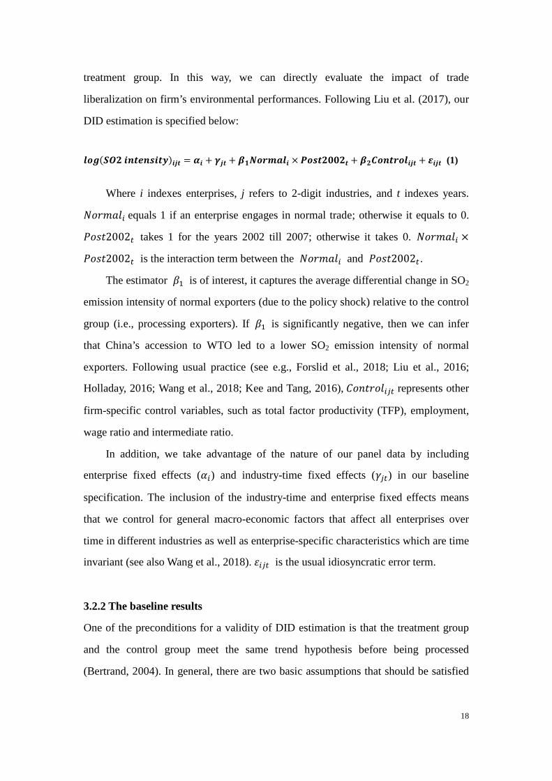
liberalization on firm’s environmental performances. Following Liu et al. (2017), our
DID estimation is specified below:
��� � ������������� = �� + ��� + ���� !�� × "���##�� + ��$������� + %��� (1)
Where i indexes enterprises, j refers to 2-digit industries, and t indexes years.
&'()*+, equals 1 if an enterprise engages in normal trade; otherwise it equals to 0.
-'./20020 takes 1 for the years 2002 till 2007; otherwise it takes 0. &'()*+, ×
-'./20020 is the interaction term between the &'()*+, and -'./20020.
The estimator 12 is of interest, it captures the average differential change in SO2
emission intensity of normal exporters (due to the policy shock) relative to the control
group (i.e., processing exporters). If 12 is significantly negative, then we can infer
that China’s accession to WTO led to a lower SO2 emission intensity of normal
exporters. Following usual practice (see e.g., Forslid et al., 2018; Liu et al., 2016;
Holladay, 2016; Wang et al., 2018; Kee and Tang, 2016), 3'4/('+,50 represents other
firm-specific control variables, such as total factor productivity (TFP), employment,
wage ratio and intermediate ratio.
In addition, we take advantage of the nature of our panel data by including
enterprise fixed effects (6,) and industry-time fixed effects (750) in our baseline
specification. The inclusion of the industry-time and enterprise fixed effects means
that we control for general macro-economic factors that affect all enterprises over
time in different industries as well as enterprise-specific characteristics which are time
invariant (see also Wang et al., 2018). 8,50 is the usual idiosyncratic error term.
3.2.2 The baseline results
One of the preconditions for a validity of DID estimation is that the treatment group
and the control group meet the same trend hypothesis before being processed
(Bertrand, 2004). In general, there are two basic assumptions that should be satisfied

19
when using the DID model, namely parallel trend assumption,7 and no association
between temporary shocks (the stochastic error) and policy dummy variables.
DID allows selection to be based on individual characteristics, as long as the
characteristics do not change with time; as such, an advantage of using DID is that it
addresses the endogeneity issue due to possible “selection bias”. The result of parallel
pre-trend hypothesis is presented below.
Figure 1: China’s dual trade regime: processing trade vs. normal trade Note: Mean values of log(SO2 emissions intensity). See Table 2 for variable definition.
Before China's accession to the WTO (i.e., before 2002), the SO2 emission intensity of
the treatment group and the control group exhibited are not statistically different. In
fact, the dynamic regression analysis (given later in Table 8) reveals that, relative to
2000, firms engaged in normal trade did not exhibit significantly lower SO2 emission
7 The DID method does not require that the treatment group and the control group are identical, and there may be some differences between the two groups; but the DID method requires that the differences are constant, i.e. the treatment group and the control group exhibit the same development trend before the implementation of the policy (or external shock).

20
intensity relative to firms engaged in processing trade in the years before China’s
WTO entry.
However, due to data availability, only two data points are available before the
policy shock. In this sense, our result is only suggestive evidence for a parallel trend
assumption. After China's accession to the WTO, the SO2 emission intensity of the
treatment group and the control group exhibited different dynamics. The DID
specification examines the differential effects of China's accession to WTO on the
SO2 emission intensity of firms engaging in the two different trade modes.
3.2.3 Empirical results based on DID specification
Table 6 shows differences in mean value of natural logarithm of SO2 emission
intensity between treatment (i.e., normal exporters) and control groups (i.e.,
processing exporters) before and after China’s WTO entry.
Table 6: Differences in mean value of natural logarithm of SO2 emission intensity between treatment (i.e., normal exporters) and control groups (i.e., processing
exporters) before and after China’s WTO entry Before After Difference DID
Control
(1)
Treated
(2)
Control
(3)
Treated
(4)
(5)=(2)-(1) (6)=(4)-(3) (7)=(6)-(5)
Whole
Sample
0.278 0.442 0.215 0.327 0.165***
(0.025)
0.113***
(0.012)
-0.052*
(0.028)
Note: Before refers to the period before China's accession to the WTO; After refers to the period after
China's accession to the WTO; Control refers to processing exporters; Treated refers to normal
exporters; Difference refers to the difference of mean value of natural logarithm of SO2 emission
intensity between normal exporters and processing exporters after China's accession to the WTO
compared with the difference between the SO2 emission intensity before China's accession to the WTO.
Standard errors in parentheses. All of the values in the last row are logarithms of SO2 emission intensity. * p < 0.1, ** p < 0.05, *** p < 0.01.
There are three general observations: first, processing exporters have lower SO2
emission intensity in the whole study period (a micro evidence supporting the
differential treatment for processing trade and normal trade in studies using macro
framework, e.g. Dietzenbacher et al., 2012); second, both types of exporters saw
emission intensity decline after China’s WTO entry (in line with the general trend of

21
China’s SO2 emission intensity declining, from 1.12t/mRMB in 2000 to
0.506t/mRMB in 2007 in all industries); third, normal exporters were affected more
than processing exporters (echoing previous studies for other outcome variables such
as TFP, see e.g. Yu, 2015). In particular, it is observed that China’s WTO entry
contributed to less SO2 emission intensity for normal traders (statistically significant
at the level of 10%, see column (7)).
Table 7: DID empirical results Log (SO2 emission intensity) (1) (2) (3) (4) (5)
�� !�� × "���##�� -0.055**
(0.028)
-0.066**
(0.028)
-0.055**
(0.027)
-0.048*
(0.027)
-0.062**
(0.027)
TFP�ACF�,50 -0.227*** -0.316*** -0.179*** -0.323***
(0.039) (0.071) (0.037) (0.073)
Log �employment�,50 -0.075*** -0.100***
(0.029) (0.030)
Log �intermediate ratio�,50 -0.096* -0.092***
(0.051) (0.051)
Log �wage ratio�,50 0.066*** 0.072***
(0.013) (0.013)
Constant 0.008
(0.143)
0.481**
(0.203)
0.082
(0.143)
0.439***
(0.160)
1.046***
(0.239)
Industry fixed * Year fixed Yes Yes Yes Yes Yes
Firm fixed Yes Yes Yes Yes Yes
n 13,641 13,641 13,641 13,641 13,641
J� 0.0006 0.0002 0.0002 0.0013 0.0013
Note: Standard errors in parentheses, clustered at firm level if not otherwise stated. * p < 0.1, ** p < 0.05, *** p < 0.01. Individual fixed effect is to exclude the influence of other unobservable factors that do not
change with the enterprise; time fixed effect is to control the influence of other unobservable factors
that do not change with the time, so as to exclude the influence of other policy factors as much as
possible; industry fixed effect is to control the influence of other unobservable factors that do not
change with the industry. The fixed effects are included to control for potential omitted
industry-year-specific variables. We control for general macro-economic factors that affect all
enterprises over time in different industries as well as enterprise-specific characteristics which are time
invariant. Industry-year fixed includes 210 different categories.
In order to partial out the effects of covariates, Table 7 highlights the results of DID
estimation of relative SO2 emission intensity change of normal exporters after China's
WTO entry, where fixed effects for firms and industry*year are always included. It is

22
found that the coefficient of �� !�� × "���##�� is negative and statistically
significant.8
We start with the specification with only the interaction term included (column
(1)), the coefficient -0.055 means that compared with the processing exporters that are
not directly affected by the WTO entry, SO2 emission intensity of normal exporters
were reduced by 5.39 percent after China's accession to WTO.9 This difference is
also economically significant (noting that, during the same period, the annual average
SO2 emission intensity in China’s manufacturing sector declined by 10.7 percent from
2000 till 2007).
Next, acknowledging the important role of productivity, employment, wage ratio
and intermediate input ratio (see e.g., Forslid et al., 2018; Liu et al., 2016; Holladay,
2016; Wang et al., 2018; Kee and Tang, 2016), these control variables were each
included in the regression. The results still hold (see column (2)-(5)). Column (5) is
our preferred estimation. As expected, firms with higher productivity, larger
employment and larger intermediate input ratio saw a decline in the emission intensity.
Whereas, firms with higher wage ratio saw a rise in the emission intensity.
Essentially, in column (5) we have excluded potential confounding explanations
stemming from scale (where we controlled for employment), technology (we
controlled for TFP), outsourcing (intermediate input ratio), as well as wage ratio and
c.p. the WTO entry contributed to an extra 6% decline of SO2 emission intensity for
normal exporting firms.10 The conclusion can be drawn with relative confidence that,
compared with the processing exporters that are not directly affected by the trade
shock (i.e., China’s WTO entry), SO2 emission intensity of normal exporters saw a
8 By adopting an alternative method to delineate trade modes (e.g., Lu et al., 2015), we also found that China's accession to the WTO contributed to statistically significant negative impact on the SO2 emission intensity of normal exporters. These additional results are available upon request to the authors. 9 Following Halvorsen and Palmquist (1980) and Kennedy (1981), the percentage is calculated as
exp(βL −2
NOL�βL�) − 1, where βL is the estimate of βL and OL�βL� is the estimate of the variance of βL.
10 We also run all the regressions with TFP estimated using OLS and OP methods, the results are essentially the same. In addition, taking advantage of the fact that there is information for the trade mode at firm level, we have re-run the estimation with clustering enterprises at the level of trade mode. The results are comparable, and for the sake of brevity are omitted from the text but available upon request.
23
reduction by as much as 6% (see column (5)) after the trade shock.
This result is in line with studies for developed economies (e.g. the US, see
Cherniwchan, 2017); however, the underlying mechanism is different. Cherniwchan
(2017) attributes the clean-up of US firms exposed more to the trade shocks via
substitution of inputs by Mexican imported materials; while in our case, the declining
of SO2 emission intensity is mainly due to technology advancement (for more details
see the following section). It is worth noting that, additional results (see Appendix A7)
indicate that only in pollution-intensive manufacture industries samples, China’s
WTO entry contributed to less SO2 emission intensity for normal traders, which is
different from the findings in Forslid et al. (2018).11
Further, the pre-2002 trend indicates whether environmental performance of
normal exporters followed the same trend before China’s WTO entry. To investigate
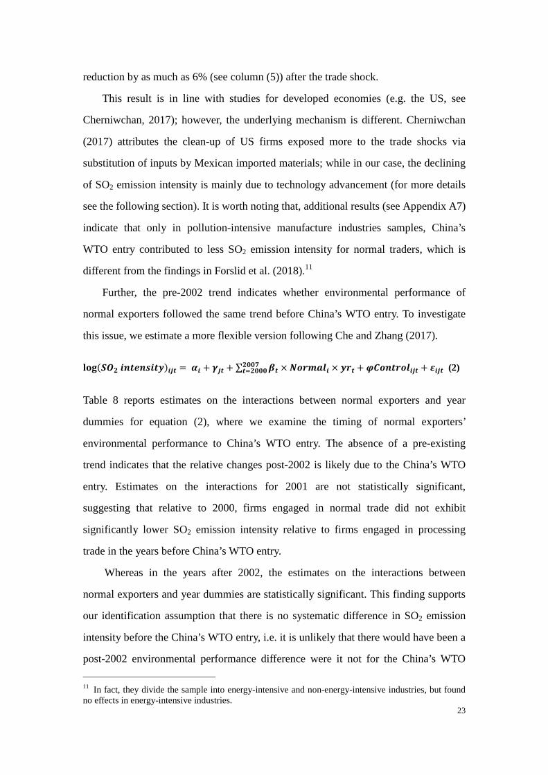
this issue, we estimate a more flexible version following Che and Zhang (2017).
QRS�� � ������������� = �� + ��� + ∑ �� × �� !�� × ��� + U$������� + %���
�##V�W�### (2)
Table 8 reports estimates on the interactions between normal exporters and year
dummies for equation (2), where we examine the timing of normal exporters’
environmental performance to China’s WTO entry. The absence of a pre-existing
trend indicates that the relative changes post-2002 is likely due to the China’s WTO
entry. Estimates on the interactions for 2001 are not statistically significant,
suggesting that relative to 2000, firms engaged in normal trade did not exhibit
significantly lower SO2 emission intensity relative to firms engaged in processing
trade in the years before China’s WTO entry.
Whereas in the years after 2002, the estimates on the interactions between
normal exporters and year dummies are statistically significant. This finding supports
our identification assumption that there is no systematic difference in SO2 emission
intensity before the China’s WTO entry, i.e. it is unlikely that there would have been a
post-2002 environmental performance difference were it not for the China’s WTO
11 In fact, they divide the sample into energy-intensive and non-energy-intensive industries, but found no effects in energy-intensive industries.

24
entry shock.
Table 8: Dynamic effects of China’s WTO entry on normal exporters’
environmental performance Log (SO2 emission intensity) (1) (2) (3) (4) (5)
&'()*+, × 2001 -0.071
(0.046)
-0.065
(0.047)
-0.059
(0.046)
-0.057
(0.047)
-0.062
(0.049)
&'()*+, × 2002 -0.092** -0.099** -0.086* -0.082* -0.095**
(0.043) (0.045) (0.043) (0.043) (0.046)
&'()*+, × 2003 -0.118** -0.122** -0.111** -0.104** -0.121**
(0.043) (0.047) (0.045) (0.043) (0.047)
&'()*+, × 2004 -0.127*** -0.136*** -0.117*** -0.108*** -0.128***
(0.040) (0.041) (0.039) (0.039) (0.041)
&'()*+, × 2005 -0.080* -0.091* -0.069 -0.055 -0.079
(0.047) (0.049) (0.046) (0.046) (0.050)
&'()*+, × 2006 -0.093** -0.106** -0.082* -0.062 -0.090*
(0.045) (0.048) (0.045) (0.044) (0.049)
&'()*+, × 2007 -0.168*** -0.195*** -0.158*** -0.152** -0.196***
(0.052) (0.054) (0.053) (0.056) (0.057)
TFP�ACF�,50 -0.226*** -0.315*** -0.178*** -0.321***
(0.053) (0.088) (0.046) (0.099)
Log �employment�,50 -0.076** -0.100***
(0.032) (0.036)
Log �intermediate ratio�,50 -0.096* -0.092
(0.054) (0.054)
Log �wage ratio�,50 0.067*** 0.072***
(0.018) (0.020)
Constant 0.053
(0.078)
0.524**
(0.218)
0.118
(0.079)
0.474***
(0.115)
1.087***
(0.311)
Industry fixed * Year fixed Yes Yes Yes Yes Yes
Firm fixed Yes Yes Yes Yes Yes
n 13,641 13,641 13,641 13,641 13,641
J� 0.0008 0.0003 0.0001 0.0011 0.0010
Note: Standard errors in parentheses. * p < 0.1, ** p < 0.05, *** p < 0.01. Individual fixed effect is to
exclude the influence of other unobservable factors that do not change with the enterprise; time fixed
effect is to control the influence of other unobservable factors that do not change with the time, so as to
exclude the influence of other policy factors as much as possible; industry fixed effect is to control the
influence of other unobservable factors that do not change with the industry. The fixed effects are
included to control for potential omitted industry-year-specific variables. We control for general
macro-economic factors that affect all enterprises over time in different industries as well as
enterprise-specific characteristics which are time invariant. Industry-year fixed includes 210 different
categories.

25
4. Mechanism test
This section proposes a potential mechanism regarding why normal exporters saw
lower emission intensity after China’s entry into WTO. Our point of departure is the
Melitz (2003) model with heterogeneous firms. Confounding policies are then
identified and discussed. Lastly, we present a further mechanism test.
4.1 Productivity channel
Previous studies have confirmed that China's accession to the WTO has significant
impact on enterprises engaged in normal trade, by increasing the total export volume
and mark-up (Brandt et al., 2017) and productivity (Yu, 2015). An additional robust
empirical finding is that processing exporters are less productive than normal
exporters, and have inferior performance in many other aspects such as profitability,
wage, R&D and skill intensity (Dai et al., 2016). Given reasonable conditions,
production volumes increase with firm productivity and, as a consequence, firms’
emission intensity is negatively related to firm productivity (Forslid et al., 2018). In
addition, trade openness increases local competition, implying that the least
productive, and usually also the most polluting, firms are forced to close down (or are
forced to scale down their production volume), thus losing market share. The Forslid
et al. (2018) model has the property that i) more productive firms are cleaner since
they find it profitable to make larger fixed investments in clean technology; ii)
exporters are cleaner for a given productivity level, since exporting implies a larger
scale of production which motivates a larger fixed investment in clean technology.
In this section, we show that these properties are largely consistent with Chinese
manufacturing survey data. As stated, the dataset contains rich information at the firm
level for a large number of variables relating to production. In line with previous
sections, the firms’ productivity is measured by TFP, and is calculated based on
Ackerberg et al. (2015).
Table 9 shows how firm-level SO2 emissions per unit of output vary with
productivity and with being a normal exporter. To account for sectoral differences in

26
emissions, we include industry dummies (two-digit industries for 28 categories); and
the year dummies are included to control for time trends. In addition, we also include
firm-level fixed effects (see also Wang et al., 2018).
Column (1) only includes the interaction term, which is interpreted as follows: for
normal exporters (compared with processing exporters), higher productivity
contributes to greater reduction of SO2 emission intensity. It is suggestive that our
proposed mechanism that China’s WTO entry contributes to normal exporting firms’
productivity (confirming previous findings, see e.g. Yu, 2015), and higher
productivity resulting in the observed lower emission intensity. Next, we explicitly
add different control variables in the regressions, and the result remains significantly
negative.12 Overall, we show that more productive normal exporters are cleaner (with
lower SO2 emission per unit of output).
Table 9: Empirical results, clustered at industry and year Log (SO2 emission intensity) (1) (2) (3) (4) (5)
�� !�� × ]^"��� -0.205***
(0.038)
-0.229***
(0.040)
-0.290***
(0.056)
-0.184***
(0.037)
-0.286***
(0.058)
Log �employment�,50 -0.071*** -0.093***
(0.022) (0.023)
Log (intermediate ratio) -0.071** -0.061**
(0.029) (0.027)
Log (wage ratio) 0.067*** 0.075***
(0.011) (0.012)
Constant 0.043
(0.122)
0.431**
(0.177)
0.065
(0.122)
0.428***
(0.135)
1.000***
(0.222)
Industry fixed * Year fixed Yes Yes Yes Yes Yes
Firm fixed Yes Yes Yes Yes Yes
Cluster Industry & Year
N 13,641 13,641 13,641 13,641 13,641
J� 0.0000 0.0003 0.0000 0.0011 0.0007
Note: Standard errors in parentheses. * p < 0.1, ** p < 0.05, *** p < 0.01. Individual fixed effect is to
exclude the influence of other unobservable factors that do not change with the enterprise; time fixed
12 Similar results are found when errors are clustered at the sector and trade mode level (available upon request). Further, in the Appendix, we extend the analysis to i) conduct falsification test via deliberately incorrectly define hybrid exporters as normal counterparts (Table A2); ii) align the analysis taking into account the environmental policy regarding pollution-intensive versus non-pollution-intensive firms (Table A4); and iii) examine potential heterogeneous effects across regions and firm ownership (Table A5) as well as ruling out trade intermediaries (Table A6).

27
effect is to control the influence of other unobservable factors that do not change with the time, so as to
exclude the influence of other policy factors as much as possible; industry fixed effect is to control the
influence of other unobservable factors that do not change with the industry. The fixed effects are
included to control for potential omitted industry-year-specific variables. We control for general
macro-economic factors that affect all enterprises over time in different industries as well as
enterprise-specific characteristics which are time invariant. Industry-year fixed includes 210 different
categories.
4.2 Ruling out confounding policies
If other policies issued before and after China's accession to the WTO that may have
different impacts on our treatment and control groups, then the effect of these policy
reforms may also be reflected in the estimates of DID.
In that case, the regression result from Eq. (1) will not be the pure effect of
China’s accession to WTO. In fact, two important reforms have taken place at the
beginning of the 2000s: the reform of state-owned enterprises (SOEs) and the
relaxation of regulations on the entry of foreign invested enterprises (FIEs).13
However, in order to control the possible confounding effects of these two policy
reforms, we add two additional control variables in our DID estimation following Liu
et al. (2016): SOEratiobc (the ratio of SOEs number to the total domestic firms
number) and Log �FIE number�bc (the logarithm of the number of foreign invested
enterprises).
The results of Table 10 show that China's accession to the WTO still has a
significantly negative impact on the SO2 emissions intensity. Our main conclusion is
still present. Firms in industries with a higher share of state-owned enterprises often
have lower SO2 emissions intensity (not statistically significant), which may be
because state-owned enterprises have a major responsibility for environmental
protection and should maintain their reputation. However, an increasing share of
13 These reforms were on-going reforms that had started in the 1980s and 1990s, respectively, and accelerated after the WTO accession. The SOE reform resulted in a large-scale privatization, close-down of small SOEs, and an improvement in the efficiency of surviving (large) SOEs. The new FDI regulations relaxed the entry requirements for foreign investors and reduced the range of industries restricted to foreign investment. These reforms may not have differentiated effects on the treatment and control groups.

28
foreign firms has c.p. no effect on the emissions intensity.
Table 10: Ruling out confounding policies Log (SO2 emission intensity) (1) (2)
�� !�� × "���##�� -0.037**
(0.002)
-0.038**
(0.001)
TFP�ACF�,50 -0.319* -0.319*
(0.034) (0.032)
Log �employment�,50 -0.095* -0.096*
(0.013) (0.013)
Log �intermediate ratio�,50 -0.087 -0.086
(0.027) (0.026)
Log �wage ratio�,50 0.076** 0.076**
(0.005) (0.006)
SOE ratio50 -0.209
(0.039)
Log �FIE number�,0 -0.002
(0.012)
Constant 1.319**
(0.096)
1.414***
(0.008)
Year fixed Yes Yes
Firm fixed Yes Yes
n 13,641 13,641
J� 0.0205 0.0220
Note: Standard errors in parentheses. * p < 0.1, ** p < 0.05, *** p < 0.01. Individual fixed effect is to
exclude the influence of other unobservable factors that do not change with the enterprise; time fixed
effect is to control the influence of other unobservable factors that do not change with the time, so as to
exclude the influence of other policy factors as much as possible.
4.3 Further mechanism check
To further investigate the impact of the productivity change of normal exporters on
their environmental performance after China's accession to WTO, we have generated
a triple interaction term �� !�� × "���##�� × ]^"��� added to Eq. (1), to
examine whether there is a differential effect that increases with TFP.
29
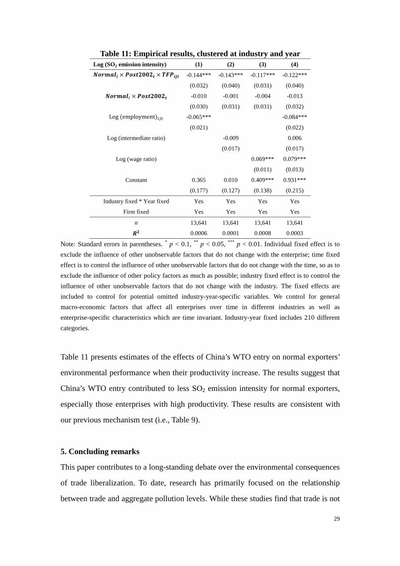
Table 11: Empirical results, clustered at industry and year Log (SO2 emission intensity) (1) (2) (3) (4)
�� !�� × "���##�� × ]^"��� -0.144*** -0.143*** -0.117*** -0.122***
(0.032) (0.040) (0.031) (0.040)
�� !�, × "���##�� -0.010
(0.030)
-0.001
(0.031)
-0.004
(0.031)
-0.013
(0.032)
Log �employment�,50 -0.065*** -0.084***
(0.021) (0.022)
Log (intermediate ratio) -0.009 0.006
(0.017) (0.017)
Log (wage ratio) 0.069*** 0.079***
(0.011) (0.013)
Constant 0.365
(0.177)
0.010
(0.127)
0.409***
(0.138)
0.931***
(0.215)
Industry fixed * Year fixed Yes Yes Yes Yes
Firm fixed Yes Yes Yes Yes
n 13,641 13,641 13,641 13,641
J� 0.0006 0.0001 0.0008 0.0003
Note: Standard errors in parentheses. * p < 0.1, ** p < 0.05, *** p < 0.01. Individual fixed effect is to
exclude the influence of other unobservable factors that do not change with the enterprise; time fixed
effect is to control the influence of other unobservable factors that do not change with the time, so as to
exclude the influence of other policy factors as much as possible; industry fixed effect is to control the
influence of other unobservable factors that do not change with the industry. The fixed effects are
included to control for potential omitted industry-year-specific variables. We control for general
macro-economic factors that affect all enterprises over time in different industries as well as
enterprise-specific characteristics which are time invariant. Industry-year fixed includes 210 different
categories.
Table 11 presents estimates of the effects of China’s WTO entry on normal exporters’
environmental performance when their productivity increase. The results suggest that
China’s WTO entry contributed to less SO2 emission intensity for normal exporters,
especially those enterprises with high productivity. These results are consistent with
our previous mechanism test (i.e., Table 9).
5. Concluding remarks
This paper contributes to a long-standing debate over the environmental consequences
of trade liberalization. To date, research has primarily focused on the relationship
between trade and aggregate pollution levels. While these studies find that trade is not

30
necessarily bad for the environment, they often appeal to the unobserved responses of
individual polluters to explain the mechanisms underlying their findings. Yet, there
has been little evidence of how trade liberalization affects the pollution from
individual manufacturing plants especially in developing countries.
This paper provides additional evidence and extends the literature in several
dimensions: First, we merged three rich firm-level datasets for China, which adds to
the empirical evidence for China, one of the most important countries in the
environment-trade debate; second, we examined the impact of trade liberalization on
China's manufacturing firms’ environmental performances with this unique dataset at
the plant level, thereby taking advantage of China’s dual trade regime (processing vs.
normal trade) and China’s WTO entry in 2001 by using a DID estimation strategy.
Third, we investigated why normal exporters saw lower emission intensity after
China’s entry into WTO pointing at the role of productive firms, echoing the channel
proposed in Melitz (2003).
Our results suggest that WTO entry played an important role in the observed
clean-up of the Chinese normal exporters in the manufacturing sector. We find that
trade liberalization following China’s accession into WTO decreased emission
intensity of sulfur dioxide from affected plants. Altogether, our estimates suggest that,
compared with the processing exporters that are not directly affected by the WTO
entry, SO2 emission intensity of normal exporters were reduced by roughly 6% due to
the trade shock. In short, China’s WTO entry contributed to less SO2 emission
intensity for normal traders, which is in line with previous evidence reported for
developed economies.
We also discuss one important mechanism that explains the observed pattern,
which is the productivity channel (motivated by Melitz, 2003 and Forslid et al., 2018).
Indeed, our results show that more productive normal exporters are cleaner (have
lower SO2 emissions per output) following China's accession to the WTO; and this
effect is more pronounced for emission-intensive industries. Future research may
focus on the explanatory power of the identified channel.
31
References
Ackerberg, D. A., K. Caves, and G. Frazer (2015). Identification Properties of Recent Production Function Estimators. Econometrica, 83(6): 2411–51.
Amiti, M., and J. Konings (2007). Trade liberalization, intermediate inputs, and productivity: evidence from Indonesia. American Economic Review, 97(5), 1611–38.
Antweiler, W., B. Copeland, and S. Taylor (2001). Is Free Trade Good for the Environment? American Economic Review, 91(4), 877-908.
Autor, D., D. Dorn, and G. Hanson (2013). The China Syndrome: Local Labor Market Effects of Import Competition in the United States, American Economic Review, 103(6), 2121-68.
Baghdadi, L., I. Zarzoso, and H. Zitouna (2013). Are RTA Agreements with Environmental Provisions Reducing Emissions? Journal of International Economics, 90, 378-390.
Batrakova, S., and R. Davies (2012). Is There an Environmental Benefit to Being an Exporter? Evidence from firm-level data, Review of World Economics, 148(3), 449-474.
Beladi, H., and R. Oladi (2010). Does Trade Liberalization Increase Global Pollution? Resource and Energy Economics, 33, 172-178.
Bernard, A., and B. Jensen (1999). Exceptional Exporter Performance: Cause, Effect, or both? Journal of International Economics, 47, 1-25.
Brandt, L., J. Biesebroeck, L. Wang, and Y. Zhang (2017). WTO Accession and Performance of Chinese Manufacturing Firms. American Economic Review, 107(9), 2784-2820.
Brandt, L., J. Biesebroeck, and Y. Zhang (2012). Creative Accounting or Creative Destruction? Firm-level Productivity Growth in Chinese Manufacturing, Journal of Development Economics, 97(2), 339-351.
Bertrand, M., E. Duflo, and S. Mullainathan (2004). How Much Should We Trust Differences-In-Differences Estimates? The Quarterly Journal of Economics, 119(1), 249-275.
Cherniwchan, J. (2017). Trade liberalization and the environment: Evidence from NAFTA and U.S. manufacturing, Journal of International Economics, 105(2017), 130-149.
Cherniwchan, J., B. Copeland, and M. Taylor (2017). Trade and the Environment: New Methods, Measurements, and Results, Annual Review of Economics, 9(1), 59-85.
Che, Y., and Z. Lei (2017). Human capital, technology adoption and firm performance: impacts of China’s higher education expansion in the late 1990s, The Economic Journal, 128(9), 2282-2320.
Cole, M., and R. Elliott (2003). Determining the Trade-Environment Composition Effect: The Role of Capital, Labor and Environmental Regulations, Journal of Environmental Economics and Management, 46(3), 363–383.
32
Cole, M., R. Elliott, and P. Fredriksson (2006). Endogenous Pollution Havens: Does FDI Influence Environmental Regulations? Scandinavian Journal of Economics, 108(1), 157-178.
Copeland, B., and S. Taylor (1994). North-South Trade and the Environment, Quarterly Journal of Economics, 109, 755-787.
Cui, J., H. Lapan, and G. Moschini (2012). Are Exporters More Environmentally Friendly than Non-Exporters? Theory and Evidence. Working Paper 12022, Iowa State University.
Dai, M., M. Maitra, and M. Yu (2016). Unexceptional exporter performance in China? The role of processing trade, Journal of Development Economics, 121, 177-189.
Dean, J. (2002). Does Trade Liberalization Harm the Environment? A New Test, Canadian Journal of Economics, 35(4), 819-842.
Dean J., and M. Lovely (2010). Trade Growth, Production Fragmentation, and China's Environment, NBER Chapters, in: China's Growing Role in World Trade, 429-469.
Dietzenbacher, E., J. Pei, and C. Yang (2012). Trade, production fragmentation, and China's carbon dioxide emissions, Journal of Environmental Economics and Management, 64(1), 88-101.
Eisenbarth, S. (2017). Is Chinese trade policy motivated by environmental concerns? Journal of Environmental Economics and Management, 82, 74-103.
Feenstra, R., Z. Li, and M. Yu (2014). Export and credit constrains under incomplete information: theory and application to China. Review of Economics and Statistics, 96(4), 729-744.
Forslid, R., T. Okubo, and K. Ulltveit-Moe (2018). Why are Firms that Export Cleaner? International Trade, Abatement and Environmental Emissions, Journal of Environmental Economics and Management, 91, 166-183.
Frankel, J., and A. Rose (2005). Is Trade Good or Bad for the Environment? Sorting out the Causality, Review of Economics and Statistics, 87(1), 85-91.
Gamper-Rabindran, S. (2006). NAFTA and the Environment: What Can the Data Tell Us? Economic Development and Cultural Change, 54(3), 605-633.
Girma, S., A. Hanley, and F. Tintelnot (2008). Exporting and the Environment: A New Look with Micro-Data, Working Paper 1423, Kiel Institute for the World Economy.
Griliches, Z., and J. Mairesse (1995). Production Functions: The Search for Identification, NBER Working Paper No. w5067.
Grossman, G., and A. Krueger (1991). Environmental Impacts of a North American Free Trade Agreement, NBER Working Paper No. 3914.
HEI (2016). Burden of disease attributable to coal-burning and other major sources of air pollution in China, Health Effects Institute, August 2016, http://pubs.healtheffects.org/view.php?id=455.
He, G., M. Fan, M. Zhou (2016). The effect of air pollution on mortality in China: Evidence from the 2008 Beijing Olympic Games, Journal of Environmental Economics and Management, 79, 18-39.
33
Hertwich, E., and G. Peters (2009). Carbon Footprint of Nations: A Global, Trade-Linked Analysis, Environmental Science & Technology, 43(16), 6414-6420.
Holladay, J. (2016). Exporters and the Environment. Canadian Journal of Economics, 49, 147-172.
Kee, H., and H. Tang (2016). Domestic Value Added in Exports: Theory and Firm Evidence from China, American Economic Review, 106(6), 1402-1436.
Klimont, Z., S. J. Smith, and J. Cofala (2013). The last decade of global anthropogenic sulfur dioxide: 2000–2011 emissions, Environmental Research Letters, 8, 014003.
Kreickemeier, U., and P. Richter (2014). Trade and the Environment: The Role of Firm Heterogeneity, Review of International Economics, 22(2), 209–225.
Leontief, W. (1970). Environmental Repercussions and the Economic Structure: An Input-Output Approach, Review of Economics and Statistics, 52(3), 262-271.
Levinsohn, J., and A. Petrin (2003). Estimating Production Functions Using Inputs to Control for Un-observables, Review of Economic Studies, 70(2), 317-341.
Liu, Q., and L. Qiu (2016). Intermediate input imports and innovations: Evidence from Chinese firms’ patent filings, Journal of International Economics, 103, 166-183.
Liu, M., R. Shadbegian, and B. Zhang (2017). Does Environmental regulation affect labor demand in China? Evidence from the textile printing and dyeing industry, Journal of Environmental Economics and Management, 86(1), 277-294.
Löschel, A., S. Rexhäuser, and M. Schymura (2013). Trade and the environment: An application of the WIOD database, Chinese Journal of Population Resources and Environment, 11(1), 51-61.
Lu, D. (2010). Exceptional Exporter Performance? Evidence from Chinese Manufacturing Firms, Chicago University, mimeo.
Lu, Y., and L. Yu (2015). Trade Liberalization and Markup Dispersion: Evidence from China’s WTO Accession. American Economic Journal: Applied Economics, 7(4), 221–53.
Managi, S., A. Hibiki, and T. Tsurumi (2009). Does trade openness improve environmental quality? Journal of Environmental Economics and Management, 58(3), 346-363.
Melitz, M.J. (2003). The impact of trade on intra-industry reallocations and aggregate industry productivity. Econometrica, 71(6), 1695-1725.
Naughton, B., and N. Lardy (1996). China’s Emergence and Prospects as a Trading Nation, Brookings Papers on Economic Activity, 1996(2), 273-344.
Olley, S., and A. Pakes (1996). The Dynamics of Productivity in The Telecommunications Equipment Industry, Econometric, 64(6), 1263-1297.
Pei, J., B. Sturm, and A. Yu (2019). Are Exporters More Environmentally Friendly? A Re-appraisal that Uses China’s Micro-data, ZEW DP #19014.
Peters, G., J. Minx, C. Weber, and O. Edenhofer (2011). Growth in Emission Transfers via International Trade from 1990 to 2008, PNAS, 108(21), 8903-8908.

34
Pierce, J., and P. Schott (2016). The Surprisingly Swift Decline of US Manufacturing Employment, American Economic Review, 106 (7), 1632-62.
Shapiro, J., and R. Walker (2018). Why Is Pollution from US Manufacturing Declining? The Roles of Environmental Regulation, Productivity, and Trade, American Economic Review, 108(12), 3814-3854.
Timmer, M. P., E. Dietzenbacher, B. Los, R. Stehrer, and G. J. de Vries (2015). An Illustrated User Guide to the World Input–Output Database: the Case of Global Automotive Production, Review of International Economics, 23: 575–605.
Tybout, J. (2001). Plant- and Firm-Level Evidence on “New” Trade Theories. NBER Working Papers 8418, National Bureau of Economic Research, Inc.
Wang, C., J. Wu, and B. Zhang (2018). Environmental regulation, emissions and productivity: Evidence from Chinese COD-emitting manufacturers, Journal of Environmental Economics and Management, 92, 54-73.
World Development Report (2020). Trading for Development in the Age of Global Value Chains, World Bank.
https://openknowledge.worldbank.org/handle/10986/32437. Xu, Y. (2011). The Use of a Goal for SO2 Mitigation Planning and Management in
China’s 11th Five-Year Plan, Journal of Environmental Planning and Management, 54(6), 769-783.
Yang, C., E. Dietzenbacher, J. Pei, X. Chen, K. Zhu, and Z. Tang (2015). Processing Trade Biases the Measurement of Vertical Specialization in China, Economic Systems Research, 26: 60-76
Yu, M. (2015). Processing trade, tariffs reductions, and firm productivity: evidence from Chinese firms, The Economic Journal, 125(6), 943-988.
Yu, M., and W. Tian (2012). China's Processing Trade: A Firm-Level Analysis, in (H. Mckay and L. Song, eds.), Rebalancing and Sustaining Growth in China, Australian National University Press, 111-148.
35
Appendix
A1. Matching and merging the datasets
Following previous research for matching and merging China’s micro data, we first
match the ASIP and the CESD. The matching and merging process is roughly divided
into two main steps (see Pei et al., 2019 for a related discussion regarding the year
2007).
Step 1: First, the ASIP and CESD databases are matched for the same year
according to enterprise name (note, duplication records are dealt with beforehand).
Second given the fact that the CESD also discloses the name an enterprise used in
previous years, the enterprise name in the remaining ASIP data sample that were not
matched in the previous step are matched with the remaining sample of CESD by
using the previously used name. Successfully matched observations are supplemented
in the original matched sample.
Step 2: Some enterprises have the same name in the ASIP database, however the
corporate code, administrative division code, telephone number, postal code and other
enterprise information may be different. Therefore, third, samples which have the
same enterprise name but different other information were screened. Likewise, there
are samples with the same enterprise name but different enterprise information in the
CESD. Based on this observation, we use the combination of enterprise name and
administration code to generate a new combination variable, and then match the
corresponding combination variable in the environmental statistics. Fourth, the
remaining ASIP database sample without being matched in the previous steps are
matched again using the combination variable generated by the name and
administration code with the environmental statistics database. Successfully matched
observations are also supplemented to samples previously obtained. Now we have the
final merged sample with both production information and environmental
performance indicators.
However, challenges remain when matching and merging the aforementioned
36
dataset with customs data. One typical issue is that ASIP data and customs data have
their own company identification numbers, and the two datasets belong to different
authorities. Consequently, one cannot merge these databases directly using enterprise
code. Following Yu and Tian (2012), we merge the two databases in two steps. First,
we merge companies with the same company name (for each year); second, we then
also merge companies with the same postal code and the same last seven digits of the
phone number. It is worth noting that, during the matching and merging process,
companies with invalid postal codes and phone numbers were excluded, i.e. 1) postal
code or phone number is lost; 2) postal code is invalid (e.g., postal code value is less
than 100000); and 3) phone number is invalid (that is, the number is less than
1000000).
Finally, our dataset is an unbalanced panel from 2000 to 2007 with 13,641
observations (plus 10,412 observations for hybrid firms; and for identification
consideration, the 13,641 observations of pure processing and normal exporters are
used in subsequent analysis, if not otherwise stated). To get a sense of the dataset, we
present three sets of information, namely the frequency distribution of survival years
and corresponding number of enterprises (given in Table A1a), the fraction of
observations matched to previous year’s firms (see Table A1b), and the dynamics of
the firms (see Table A1c).
According to the statistics, there are 7,822 (resp. 6,004) enterprises included in
the unbalanced panel (resp. hybrid firms) in the period of 2000-2007.

37
Table A1a: Survival years and the number of firms
Survival Years Number of enterprises (pure
normal & processing exporters)
Number of enterprises (Hybrid)
1 4,543 3,974
2 1,776 965
3 880 513
4 344 275
5 170 135
6 83 84
7 26 44
8 0 14
Total 7,822 6,004
Observations 13,641 10,142
Source: Authors’ own calculation based on the matched dataset.
Further, unique firms’ IDs enable us to link firms over time.14 In our context, it is
important to be able to link subsequent observations of the same firm even when the
firm ID changed. In this way, it is possible to understand the dynamics of entry and
exit of firms. Table A1b reports the percentage of firms that are matched each year on
the basis of firm ID and those matched using other information. The total proportion
of successfully matched enterprises, for example, in 2000-2001 is 27.28%, and 25.49%
in 2006-2007. Overall, the proportion of matched firms is rather stable over time.
14 Firms occasionally receive a new ID if they encounter restructuring, merger and/or acquisition. Following Brandt et al. (2012), we linked and also tracked firms as their boundaries or ownership structure changed, where possible, using information such as firm name, industry, phone number, post, etc. Many incumbents were restructured or privatized and we want to make sure not to lump these with exiting firms or classify them as de novo entrants under their new firm ID.
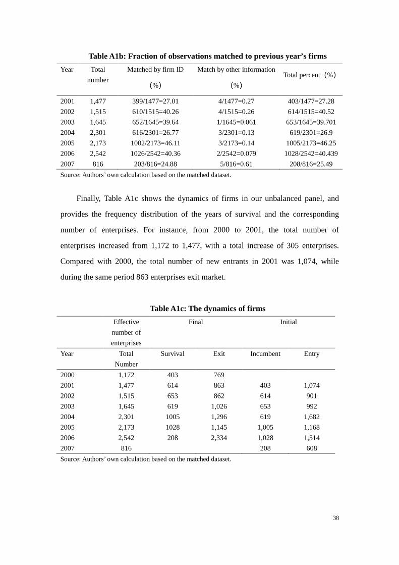
38
Table A1b: Fraction of observations matched to previous year’s firms
Year Total
number
Matched by firm ID
(%)
Match by other information
(%)
Total percent(%)
2001 1,477 399/1477=27.01 4/1477=0.27 403/1477=27.28
2002 1,515 610/1515=40.26 4/1515=0.26 614/1515=40.52
2003 1,645 652/1645=39.64 1/1645=0.061 653/1645=39.701
2004 2,301 616/2301=26.77 3/2301=0.13 619/2301=26.9
2005 2,173 1002/2173=46.11 3/2173=0.14 1005/2173=46.25
2006 2,542 1026/2542=40.36 2/2542=0.079 1028/2542=40.439
2007 816 203/816=24.88 5/816=0.61 208/816=25.49
Source: Authors’ own calculation based on the matched dataset.
Finally, Table A1c shows the dynamics of firms in our unbalanced panel, and
provides the frequency distribution of the years of survival and the corresponding
number of enterprises. For instance, from 2000 to 2001, the total number of
enterprises increased from 1,172 to 1,477, with a total increase of 305 enterprises.
Compared with 2000, the total number of new entrants in 2001 was 1,074, while
during the same period 863 enterprises exit market.
Table A1c: The dynamics of firms
Effective
number of
enterprises
Final Initial
Year Total
Number
Survival Exit
Incumbent
Entry
2000 1,172 403 769
2001 1,477 614 863 403 1,074
2002 1,515 653 862 614 901
2003 1,645 619 1,026 653 992
2004 2,301 1005 1,296 619 1,682
2005 2,173 1028 1,145 1,005 1,168
2006 2,542 208 2,334 1,028 1,514
2007 816 208 608
Source: Authors’ own calculation based on the matched dataset.

39
Robustness check 1: Replacing normal trade with hybrid trade
As explained previously, there are enterprises engaged in both normal trade and
processing trade, and we termed these enterprises as hybrid firms. In theory, if we
have a ranking for the firms that are directly affected by trade shocks, it is reasonable
to consider that the normal exporting firms would be the most affected by China's
accession to the WTO, and the processing exporters would be the least, while the
hybrid firms lie in between (i.e., ambiguous or insignificant effects are expected).
Table A2: DID Results: falsification test
Log (SO2 emission intensity) (1) (2) (3) (4) (5)
g�h��i� × "���##�� -0.011
(0.014)
-0.012
(0.014)
-0.011
(0.014)
-0.010
(0.014)
-0.010
(0.014)
TFP�ACF�,50 -0.079** -0.213*** -0.055* -0.225***
(0.031) (0.064) (0.030) (0.068)
Log �employment�,50 -0.033*** -0.049***
(0.012) (0.013)
Log �intermediate ratio�,50 -0.121*** -0.125***
(0.044) (0.046)
Log �wage ratio�,50 0.036*** 0.035***
(0.011) (0.011)
Constant 0.322
(0.200)
0.556**
(0.229)
0.366*
(0.202)
0.513***
(0.187)
0.810***
(0.195)
Industry fixed * Year fixed Yes Yes Yes Yes Yes
Firm fixed Yes Yes Yes Yes Yes
N 11,908 11,908 11,908 11,908 11,908
J� 0.0021 0.0033 0.0041 0.0034 0.0055
Note: Standard errors in parentheses. * p < 0.1, ** p < 0.05, *** p < 0.01. Individual fixed effect is to
exclude the influence of other unobservable factors that do not change with the enterprise; time fixed
effect is to control the influence of other unobservable factors that do not change with the time, so as to
exclude the influence of other policy factors as much as possible; industry fixed effect is to control the
influence of other unobservable factors that do not change with the industry. The fixed effects are
included to control for potential omitted industry-year-specific variables. We control for general
macro-economic factors that affect all enterprises over time in different industries as well as
enterprise-specific characteristics which are time invariant. Industry-year fixed includes 204 different
categories.
Empirically, we deliberately replace the normal exporters using the hybrid firms and
re-run the regression (similar to a falsification test). The results are shown in Table A2.
40
We observe that China's accession to the WTO also contributed to lower SO2 emission
intensity for hybrid firms, however, the result is not statistically significant.
Robustness check 2: pollution intensity
According to the First National Pollution Source Census Program issued by the State
Council, we divide the manufacturing industry into pollution-intensive industry and
non-pollution-intensive industry. The pollution-intensive industries include the key
pollution industries and key monitoring industries, while the non-pollution-intensive
industry includes all other industries (State Council, 2007, see Table A3).
To allow for variation between the pollution-intensive industries and
non-pollution-intensive industries, we re-estimate equation (1) in Section 3.2 of the
paper by splitting the sample into pollution-intensive industries and
non-pollution-intensive industries. The results are reported for both groups of
industries in Table A4.

41
Table A3: Classification of manufacture industries Pollution-intensive industries Non-pollution-intensive industries
Heavy Pollution Industries Key Monitoring Industries
processing of food from
agricultural products (13)
manufacture of textile wearing
apparel, footwear, and caps (18)
manufacture of furniture (21)
manufacture of food (14) processing of timbers, manufacture of
wood, bamboo, rattan products (20)
manufacture of articles for culture,
education and sport act (24)
manufacture of textile (17) manufacture of general purpose
machinery (35)
manufacture of plastic (30)
manufacture of leather, fur,
feather and its products (19)
manufacture of special purpose
machinery (36)
manufacture of paper and
paper products (22)
manufacture of transport equipment
(37)
manufacture of tobacco (16)
processing of petroleum,
coking, processing of
nucleus fuel (25)
manufacture of communication
equipment, computer and other
electronic equipment (40)
printing reproduction of recording media
(23)
manufacture of chemical
raw material and chemical
products (26)
manufacture of beverage (15) manufacture of electrical machinery and
equipment (39)
manufacture of non-metallic
mineral products (31)
manufacture of metal products (34) manufacture of measuring instrument and
machinery for culture and office (41)
manufacture and processing
of ferrous metal (32)
manufacture of medicines (27) manufacture of artwork, other
manufacture (42)
manufacture and processing
of non-ferrous metals (33)
manufacture of chemical fiber (28)
recycling and disposal of waste (43)
manufacture of rubber (29)
Note: The figures in parentheses are the large-size industry codes of industries, corresponding to the national
industry classification issued by the National Bureau of Statistics of China (GB/T 4754-2002).
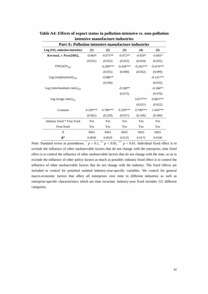
42
Table A4: Effects of export status in pollution-intensive vs. non-pollution intensive manufacture industries
Part A: Pollution intensive manufacture industries Log (SO2 emission intensity) (1) (2) (3) (4) (5)
�� !�� × "���##�� -0.064*
(0.031)
-0.075**
(0.032)
-0.072**
(0.032)
-0.059*
(0.034)
-0.065*
(0.035)
TFP�ACF�,50 -0.294*** -0.458*** -0.242*** -0.474***
(0.055) (0.090) (0.052) (0.099)
Log �employment�,50 -0.086** -0.121***
(0.036) (0.035)
Log �intermediate ratio�,50 -0.168** -0.166**
(0.075) (0.070)
Log �wage ratio�,50 0.077*** 0.083***
(0.021) (0.022)
Constant 0.250***
(0.062)
0.786***
(0.229)
0.359***
(0.057)
0.749***
(0.106)
1.456***
(0.300)
Industry fixed * Year fixed Yes Yes Yes Yes Yes
Firm fixed Yes Yes Yes Yes Yes
N 9455 9455 9455 9455 9455
J� 0.0030 0.0029 0.0125 0.0172 0.0100
Note: Standard errors in parentheses. * p < 0.1, ** p < 0.05, *** p < 0.01. Individual fixed effect is to
exclude the influence of other unobservable factors that do not change with the enterprise; time fixed
effect is to control the influence of other unobservable factors that do not change with the time, so as to
exclude the influence of other policy factors as much as possible; industry fixed effect is to control the
influence of other unobservable factors that do not change with the industry. The fixed effects are
included to control for potential omitted industry-year-specific variables. We control for general
macro-economic factors that affect all enterprises over time in different industries as well as
enterprise-specific characteristics which are time invariant. Industry-year fixed includes 121 different
categories.
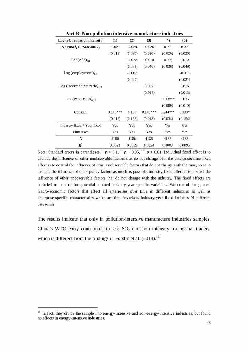
43
Part B: Non-pollution intensive manufacture industries
Log (SO2 emission intensity) (1) (2) (3) (4) (5)
�� !�� × "���##�� -0.027
(0.019)
-0.028
(0.020)
-0.026
(0.020)
-0.025
(0.020)
-0.029
(0.020)
TFP�ACF�,50 -0.022 -0.010 -0.006 0.010
(0.033) (0.046) (0.036) (0.049)
Log �employment�,50 -0.007 -0.013
(0.020) (0.021)
Log �intermediate ratio�,50 0.007 0.016
(0.014) (0.013)
Log �wage ratio�,50 0.033*** 0.035
(0.009) (0.010)
Constant 0.145***
(0.018)
0.195
(0.132)
0.143***
(0.018)
0.244***
(0.034)
0.333*
(0.154)
Industry fixed * Year fixed Yes Yes Yes Yes Yes
Firm fixed Yes Yes Yes Yes Yes
N 4186 4186 4186 4186 4186
J� 0.0023 0.0029 0.0024 0.0083 0.0095
Note: Standard errors in parentheses. * p < 0.1, ** p < 0.05, *** p < 0.01. Individual fixed effect is to
exclude the influence of other unobservable factors that do not change with the enterprise; time fixed
effect is to control the influence of other unobservable factors that do not change with the time, so as to
exclude the influence of other policy factors as much as possible; industry fixed effect is to control the
influence of other unobservable factors that do not change with the industry. The fixed effects are
included to control for potential omitted industry-year-specific variables. We control for general
macro-economic factors that affect all enterprises over time in different industries as well as
enterprise-specific characteristics which are time invariant. Industry-year fixed includes 91 different
categories.
The results indicate that only in pollution-intensive manufacture industries samples,
China’s WTO entry contributed to less SO2 emission intensity for normal traders,
which is different from the findings in Forslid et al. (2018).15
15 In fact, they divide the sample into energy-intensive and non-energy-intensive industries, but found no effects in energy-intensive industries.

44
Robustness check 2: Heterogeneous effects of regional structure and ownership Do the effects vary across regions?
There may be reasons to suspect that the effects of China’s WTO entry on normal
exporters’ environmental performance vary across regions. Because of the different
level of economic development in different regions, they have different degrees of
environmental protection, coupled with region-specific characteristics. According to
the classification of the central government, the address codes in our sample can be
divided into four regions: eastern, central, western and northeastern. The sub-samples
of the eastern region are larger than those of other regions, so we merge the samples
of three regions except the eastern region into one sample (other regions) for analysis
(see analogous treatment in Wang et al., 2018).
Do the effects vary by ownership?
One important feature of the Chinese economy is that state owned enterprises (SOEs),
other domestic enterprises, Hong Kong, Macao, Taiwan (HMT) invested enterprises
and foreign invested enterprises (FIEs) may face different incentives and constraints,
which may lead to different responses during China’s entry to WTO. Ownership may
also affect an enterprise's response to environmental regulations. Pargal and Wheeler
(1996) find that the marginal abatement cost of state-owned enterprises is higher than
that of private firms. By comparing the environmental performance of enterprises
with different ownership types, some studies have also found that multinational
enterprises are more inclined to have clean technology than other types of enterprises.
Developed countries usually have higher environmental standards than developing
countries, so this is more conducive to the innovation and development of
environment-friendly technologies in developed countries (Lanjouw and Mody,
1996).
Therefore, even where standards are relatively weak, foreign-invested enterprises
often adopt newer and cleaner technologies. Domestic enterprises in many developing
countries do not have enough funds to acquire environmental technologies to cope

45
with new entrants and foreign competition (Christmann and Taylor, 2001).
Multinational corporations usually face greater environmental protection pressures.
The institutional pressure of environmental self-regulation of multinational
corporations stems from a complex legal environment, including supranational
institutional pressure (Kostova and Zaheer, 1999).
Customers and the public may be much less tolerant of foreign companies'
misconduct than domestic companies, and in terms of bargaining power, foreign
companies may be weaker than domestic companies (Lin et al., 2014). Companies
with different ownership structures have different bargaining power in enforcing
environmental regulations, such as pollution charges and fines (Wang and Wheeler,
2003). Foreign companies are often the target of regulatory enforcement as they are
not familiar with the local political background.
In sum, to check whether the effects of China’s WTO entry on normal exporters’
environmental performance vary across ownership in different regions, one reference
is specified (i.e., other domestic firms). The results are reported in Table A5.
It is found that in Eastern regions, China’s WTO entry contributed to lower SO2
emissions intensity for normal exporters when the enterprise is state owned enterprise
(statistically significant at 10% level); for foreign invested normal exporters, China’s
WTO entry contributed to higher SO2 emissions intensity; while for HMT invested
normal exporters, there is no statistical significance; all compared with domestic other
firms. It is noted that, for China’s 11th Five-Year-Plan starting from 2006 till 2010, the
binding SO2 reduction targets (nation-wide is 10% lower in 2010 compared with 2005)
for eastern regions (e.g., Shanghai need to reduce 26%) are more ambitious than other
regions (e.g., Inner Mongolia for less than 4%); this could be one of the reasons but
should only play out after 2006. While in other regions, China’s WTO entry
contributed to higher SO2 emission intensity for normal exporters, in particular, when
the enterprise is state owned.
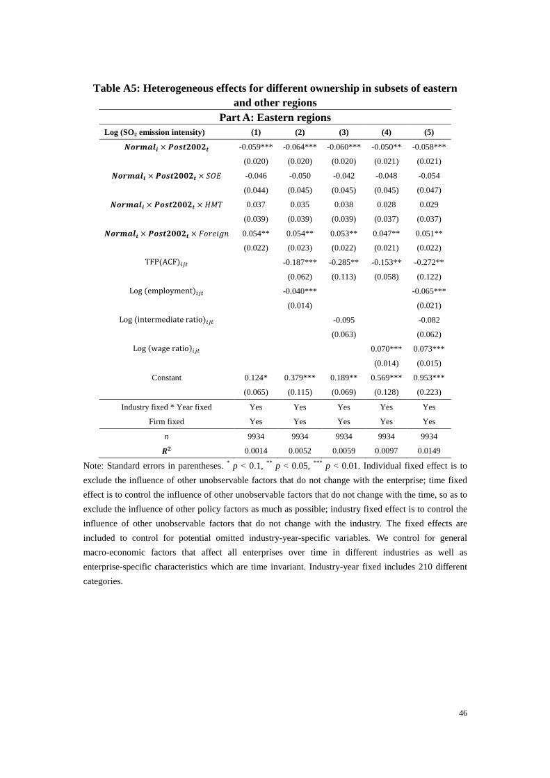
46
Table A5: Heterogeneous effects for different ownership in subsets of eastern
and other regions Part A: Eastern regions
Log (SO2 emission intensity) (1) (2) (3) (4) (5)
�� !�� × "���##�� -0.059***
(0.020)
-0.064***
(0.020)
-0.060***
(0.020)
-0.050**
(0.021)
-0.058***
(0.021)
�� !�� × "���##�� × jkl -0.046 -0.050 -0.042 -0.048 -0.054
(0.044) (0.045) (0.045) (0.045) (0.047)
�� !�� × "���##�� × mno 0.037 0.035 0.038 0.028 0.029
(0.039) (0.039) (0.039) (0.037) (0.037)
�� !�� × "���##�� × p'(qrs4 0.054** 0.054** 0.053** 0.047** 0.051**
(0.022) (0.023) (0.022) (0.021) (0.022)
TFP�ACF�,50 -0.187*** -0.285** -0.153** -0.272**
(0.062) (0.113) (0.058) (0.122)
Log �employment�,50 -0.040*** -0.065***
(0.014) (0.021)
Log �intermediate ratio�,50
-0.095
(0.063)
-0.082
(0.062)
Log �wage ratio�,50
0.070***
(0.014)
0.073***
(0.015)
Constant 0.124*
(0.065)
0.379***
(0.115)
0.189**
(0.069)
0.569***
(0.128)
0.953***
(0.223)
Industry fixed * Year fixed Yes Yes Yes Yes Yes
Firm fixed Yes Yes Yes Yes Yes
n 9934 9934 9934 9934 9934
J� 0.0014 0.0052 0.0059 0.0097 0.0149
Note: Standard errors in parentheses. * p < 0.1, ** p < 0.05, *** p < 0.01. Individual fixed effect is to
exclude the influence of other unobservable factors that do not change with the enterprise; time fixed
effect is to control the influence of other unobservable factors that do not change with the time, so as to
exclude the influence of other policy factors as much as possible; industry fixed effect is to control the
influence of other unobservable factors that do not change with the industry. The fixed effects are
included to control for potential omitted industry-year-specific variables. We control for general
macro-economic factors that affect all enterprises over time in different industries as well as
enterprise-specific characteristics which are time invariant. Industry-year fixed includes 210 different
categories.

47
Part B: Other regions Log (SO2 emission intensity) (1) (2) (3) (4) (5)
�� !�� × "���##�� 0.127
(0.174)
0.134
(0.171)
0.133
(0.172)
0.141
(0.174)
0.124
(0.175)
�� !�� × "���##�� × jkl 0.120** 0.111** 0.113** 0.111** 0.111**
(0.049) (0.048) (0.050) (0.051) (0.049)
�� !�� × "���##�� × mno 0.070 0.087 0.061 0.056 0.068
(0.132) (0.127) (0.130) (0.134) (0.134)
�� !�� × "���##�� × p'(qrs4 0.104 0.122* 0.097 0.092 0.113
(0.084) (0.070) (0.083) (0.087) (0.078)
TFP�ACF�,50 -0.266** -0.356*** -0.190* -0.452**
(0.116) (0.108) (0.109) (0.166)
Log �employment�,50 -0.186 -0.207*
(0.114) (0.116)
Log �intermediate ratio�,50
-0.122**
(0.052)
-0.162**
(0.062)
Log �wage ratio�,50 0.045
(0.053)
0.053
(0.053)
Constant 0.534***
(0.154)
1.630**
(0.703)
0.640***
(0.168)
0.717**
(0.284)
2.075**
(0.862)
Industry fixed * Year fixed Yes Yes Yes Yes Yes
Firm fixed Yes Yes Yes Yes Yes
n 3707 3707 3707 3707 3707
J� 0.0001 0.0002 0.0006 0.0010 0.0001
Note: Standard errors in parentheses. * p < 0.1, ** p < 0.05, *** p < 0.01. Individual fixed effect is to
exclude the influence of other unobservable factors that do not change with the enterprise; time fixed
effect is to control the influence of other unobservable factors that do not change with the time, so as to
exclude the influence of other policy factors as much as possible; industry fixed effect is to control the
influence of other unobservable factors that do not change with the industry. The fixed effects are
included to control for potential omitted industry-year-specific variables. We control for general
macro-economic factors that affect all enterprises over time in different industries as well as
enterprise-specific characteristics which are time invariant. Industry-year fixed includes 195 different
categories.
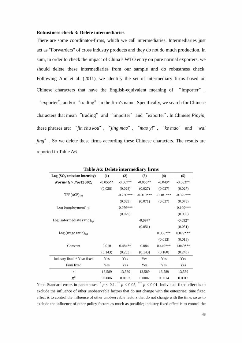
48
Robustness check 3: Delete intermediaries
There are some coordinator-firms, which we call intermediaries. Intermediaries just
act as "Forwarders" of cross industry products and they do not do much production. In
sum, in order to check the impact of China’s WTO entry on pure normal exporters, we
should delete these intermediaries from our sample and do robustness check.
Following Ahn et al. (2011), we identify the set of intermediary firms based on
Chinese characters that have the English-equivalent meaning of “ importer” ,
“exporter”, and/or “trading” in the firm's name. Specifically, we search for Chinese
characters that mean “trading” and “importer” and “exporter”. In Chinese Pinyin,
these phrases are: “jin chu kou”, “jing mao”, “mao yi”, “ke mao” and “wai
jing”. So we delete these firms according these Chinese characters. The results are
reported in Table A6.
Table A6: Delete intermediary firms Log (SO2 emission intensity) (1) (2) (3) (4) (5)
�� !�� × "���##�� -0.055**
(0.028)
-0.067**
(0.028)
-0.055**
(0.027)
-0.049*
(0.027)
-0.063**
(0.027)
TFP�ACF�,50 -0.230*** -0.319*** -0.181*** -0.325***
(0.039) (0.071) (0.037) (0.073)
Log �employment�,50 -0.076*** -0.100***
(0.029) (0.030)
Log �intermediate ratio�,50 -0.097* -0.092*
(0.051) (0.051)
Log �wage ratio�,50 0.066*** 0.072***
(0.013) (0.013)
Constant 0.010
(0.143)
0.484**
(0.203)
0.084
(0.143)
0.440***
(0.160)
1.049***
(0.240)
Industry fixed * Year fixed Yes Yes Yes Yes Yes
Firm fixed Yes Yes Yes Yes Yes
n 13,589 13,589 13,589 13,589 13,589
J� 0.0006 0.0002 0.0002 0.0014 0.0013
Note: Standard errors in parentheses. * p < 0.1, ** p < 0.05, *** p < 0.01. Individual fixed effect is to
exclude the influence of other unobservable factors that do not change with the enterprise; time fixed
effect is to control the influence of other unobservable factors that do not change with the time, so as to
exclude the influence of other policy factors as much as possible; industry fixed effect is to control the
49
influence of other unobservable factors that do not change with the industry. The fixed effects are
included to control for potential omitted industry-year-specific variables. We control for general
macro-economic factors that affect all enterprises over time in different industries as well as
enterprise-specific characteristics which are time invariant. Industry-year fixed includes 210 different
categories.
References
Ahn J., A. Khandelwal, and S. Wei (2011). The Role of Intermediaries in Facilitating Trade, Journal of International Economics, 84(1), 73-85.
Che, Y., and Z. Lei (2017). Human capital, technology adoption and firm performance: impacts of China’s higher education expansion in the late 1990s, The Economic Journal, 128(9), 2282-2320.
Christmann, P., and G. Taylor (2001). Globalization and the Environment: Determinants of Firm Self-Regulation in China, Journal of International Business Studies, 32(3), 439-458.
Kostova, T., and S. Zaheer (1999). Organizational Legitimacy under Conditions of Complexity: The Case of the Multinational Enterprise, The Academy of Management Review, 24(1), 64-81.
Lanjouw, J., and A. Mody (1996). Innovation and the international diffusion of environmentally responsive technology, Research Policy, 25(4), 549-571.
Lin, L., J. Moon, and H. Yin (2014). Does International Economic Integration Lead to a Cleaner Production in China? Production and Operations Management, 23(4), 525-536.
Pargal, S., and D. Wheeler (1996). Informal Regulation of Industrial Pollution in Developing Countries: Evidence from Indonesia, Journal of Political Economy, 104(6), 1314-27.
State Council (2007). Notice of the State Council on Launching the First National Pollution Source Survey. Beijing (in Chinese).
Wang, H., and D. Wheeler (2003). Equilibrium pollution and economic development in China, Environment and Development Economics, 8(3), 451-466.
Wang, C., J. Wu, and B. Zhang (2018). Environmental regulation, emissions and productivity: Evidence from Chinese COD-emitting manufacturers, Journal of Environmental Economics and Management, 92, 54-73.

ZEW – Leibniz-Zentrum für Europäische Wirtschaftsforschung GmbH MannheimZEW – Leibniz Centre for European Economic Research
L 7,1 · 68161 Mannheim · Germany Phone +49 621 1235-01 [email protected] · zew.de
Discussion Papers are intended to make results of ZEW research promptly avail able to other economists in order to encourage discussion and suggestions for revisions. The authors are solely respons ible for the contents which do not necessarily represent the opinion of the ZEW.
IMPRINT
//
Download ZEW Discussion Papers from our ftp server:
http://ftp.zew.de/pub/zew-docs/dp/
or see:
https://www.ssrn.com/link/ZEW-Ctr-Euro-Econ-Research.html https://ideas.repec.org/s/zbw/zewdip.html