FUTA Journal of Management and Technology Effect of Exchange Volatility on Export Volume Vol.1, No. 2 December 2016 A. Adaramola
45
THE EFFECT OF REAL EXCHANGE RATE VOLATILITY ON EXPORT
VOLUME IN NIGERIA
A. Adaramola
Department of Banking and Finance
Ekiti State University
Ado-Ekiti, Nigeria
Abstract
This paper examined the effect of real exchange rate volatility on export volumes in Nigeria.
The study employed the time series quarterly data for the period of 1970Q1-2014Q4. The
analytical method employed was econometric techniques of Johansen Multivariate approach
to co-integration as well as the Error Correction Mechanism (ECM). The study also
employed the ARCH and GARCH model to determine the presence of volatility in the real
exchange rate series. The real export volumes, real exchange rate as well as real exchange
rate volatility and all other orthodox determinants of export such as relative price and real
foreign income series were non-stationary. They were indeed I (1) series. The estimated
result indicated that there was a long run relationship between real exchange rate and its
volatility and export volumes in Nigeria. The ARCH and GARCH model showed that the
exchange rate was volatile. The paper concluded that real exchange rate uncertainty had
significantly and positively impacted on the volume of trade of the Nigerian economy. It was
therefore recommended that the monetary authorities in Nigeria should initiate policies and
programme that would stabilize naira exchange rate and remove the negative effect of
exchange rate fluctuations on Nigeria’s export performance.
Keywords: Real Exchange Rate, Export Income, Volatility, J-Curve.
1. Introduction
Export earnings assume vital importance not only for developing, but also for developed
countries. Developed countries mainly export capital and final goods, while the main part of
the export of developing countries consists of mining-industry goods, especially natural
resources (Obadan, 2006). According to export-led growth hypothesis, increased export can
perform the role of “engine of economic growth” because it can increase employment, create
profit, trigger greater productivity and lead to rise in accumulation of reserves, allowing a
country to balance their finances (Emilio (2001), Goldstein & Pevehouse (2008), Gibson &
Michael (1992), McCombie & Thirlwall (1994)).
However, exchange rate fluctuation is of interest because of its adverse effects on export
trade. More particularly, economists are interested in the operations involved in exchange
rate especially in developing countries. Real exchange rate uncertainty is said to probably
have a negative effect on international trade as bilateral trades are threatened with the risks
involved. The economic relationship supporting the negative link is the unwillingness of
firms to take on risky activity, namely trade (Anderton & Skudely, 2001).
Aliyu (2008) stated that the conception behind exchange rates is not exclusively as an
important relative price, which creates a correlation between the domestic market and the
world market for goods and assets, but as well distinguishes the competitiveness of a
country’s exchange power vis-à-vis the rest of the world in a pure market. It also sustains the
internal and external macroeconomic balances over the medium-to-long term.
FUTA Journal of Management and Technology Effect of Exchange Volatility on Export Volume Vol.1, No. 2 December 2016 A. Adaramola
46
Since the adoption of a floating exchange-rate regime in 1973 in Nigeria, the effects of
exchange-rate volatility on the volume of international trade have been the subjects of both
theoretical and empirical investigations (Obadan, 2006). Exchange rate volatility is defined
as the risk associated with unexpected movements in the exchange rate. Economic
fundamentals such as the inflation rate, interest rate and the balance of payments, which
have become more volatile in the past three decades are sources of exchange rate volatility.
The high degree of volatility and uncertainty of exchange rate movements since the
beginning of the generalized floating in 1973 has led policy makers and researchers to
investigate the nature and extent of the impact of such movements on the volume of trade.
The lack of certainty regarding economic variables that influence production is a problem
that characterizes the productive sector in general and is discussed in the literature both on
the level of the firm and on the level of aggregate investment. The path-breaking article by
Hartman (1972) tested the effect of uncertainty on the firm’s production decision. Since
then, interest has grown on the effect of uncertainty (of various types: ranging from
economy-wide uncertainty to price uncertainty and industry-wide shocks) on various
components of demand and in particular on private consumption and investment. Studies
have been carried out under various assumptions regarding the degree of risk aversion
among individuals and firms, i.e. under the assumption that individuals and firms are risk
averse or alternatively that they are risk indifferent.
The past several decades have witnessed considerable research concerning the impact of
exchange-rate volatility on the volume of international trade, and much has been written on
both the theoretical and empirical sides of this issue. Nonetheless, there is no real consensus
about the effects of real exchange rate on trade volume. Therefore, this research work is to
present additional evidence about the influence of real exchange rate uncertainty on exports,
using data for the developing economy of Nigeria.
Nigeria benefits when there is an increase in the price of oil and experiences a decline in the
value of her currency against the US dollar as a large volume of revenues is from oil export
and at the same time, the country is spending significant resources to import refined
petroleum and other oil related products which are basically traded in US dollars. The naira
exchange rate has witnessed some period of relative calm since the Implementation of the
Structural Adjustment Programme (SAP) in July, 1986; its continued depreciation, however,
scored an indelible mark in the level of real sector activities in the country. The naira which
traded at N0.935 = 1.00USD in 1985 depreciated to N2.413 = 1.00USD and further to
N7.901 against the US dollar in 1990. The naira as since depreciated from N21.886 = 1.00
USD to N142.00 = 1 USD between the period of 1994 to 2009 as a result of pegging and
further deregulation. It majorly declined by 12.95% and a further decline of 7.98% in 2008
and 2009 respectively. In spite of these developments, the national income accounts, for the
country revealed an impressive performance. Real GDP grew at an average of 5.01 percent
between 2000 and 2008 with the highest of 9.6 percent in 2003 (CBN Statistical Bulletin,
2010).
McKenzie (1999) and Clark, Tamirisa and Wei, (2004) are amongst notable scholars to have
analyzed the relationship between exchange rate volatility and international trade. They
concluded that there was a boom in international trade as a result of balance to the exchange
market. McKenzie (1999) further stated that there were theoretical models which supported
both negative and positive relationship between exchange rate volatility and international

FUTA Journal of Management and Technology Effect of Exchange Volatility on Export Volume Vol.1, No. 2 December 2016 A. Adaramola
47
trade. This shows that there is no consensus among scholars on the relationship between
exchange rate volatility and international trade, whether in the developed economies or the
developing ones. Moreover, most of the theories as well as the empirical studies on the
subject of real exchange rate uncertainty and its effect on exports are concentrated in the
developed countries. It is against this background that this paper seeks to measure the effect
of real exchange rate volatility on export volume in Nigeria.
2. Literature Review
2.1 Theoretical Literature
Clark’s (1973) model is one of the earliest theories that examined the connection between
exchange rate volatility and trade flows. The model makes several assumptions. First, the
firm has no market power, produces only one commodity which is sold entirely to one
foreign market and does not import any intermediate inputs. Second, payment is made to
this firm in foreign currency and the proceeds of its exports are converted at the current
exchange rate. In addition, the exchange rate is unpredictable and there are no hedging
possibilities. Lastly, the firm makes its production decision in advance because of the
exchange rate and therefore cannot alter its output in response to favourable or unfavourable
shifts in the profitability of its exports arising from fluctuations in the exchange rate. From
this scenario, Clark posited that the variability in the firm’s profits arises solely from the
exchange rate, and where the managers of the firm are adversely affected by risk, greater
volatility in the exchange rate – with no change in its average level leads to a reduction in
output, and hence in exports, in order to reduce the exposure to risk. This position was
corroborated by Hooper and Kohlhagen (1978) who also reached the same conclusion of a
clear negative relationship between exchange rate volatility and the level of trade. On the
other hand, Barkoulas, Baum & Caglayan (2002) developed a model in which exchange rate
volatility had positive effect on exports. However, the effect became negative when the
assumption of the existence of the forward exchange market is relaxed.
According to the J-Curve theory, depreciation of the national currency leads to serious
deterioration of the trade balance which is later followed by an improvement. A price effect
occurs immediately after the depreciation due to higher prices of imported goods and this
specifically affects inputs that are sourced from foreign countries. However, when traders
have had some time to change their input strategy, they integrate their loss in
competitiveness vis-à-vis goods produced abroad. This leads to what is termed the quantity
effect. The latter effect adjusts the volume of imports downward while local production
increases significantly. The final effect in the longer term is a net improvement in the trade
balance. This phenomenon is named the J-curve effect because when a country’s net trade
balance is plotted on the vertical axis and time is plotted on the horizontal axis, the response
of the trade balance to a devaluation or depreciation looks like the curve of the letter J. This
is shown in Fig. 2.1:
Fig. 2.1: The J-Curve

FUTA Journal of Management and Technology Effect of Exchange Volatility on Export Volume Vol.1, No. 2 December 2016 A. Adaramola
48
Marshall–Lerner theory used the J-Curve to explain why a reduction in value of a nation's
currency need not immediately improve its balance of payments. According to the theory,
for a currency depreciation to have a positive impact on the trade balance, the sum of price
elasticity of exports and imports in absolute value must be greater than one. Since a
devaluation or depreciation of the exchange rate implies a reduction in the price of exports,
the quantity exported will increase. At the same time, the price of imports will rise and their
quantity demanded will diminish. The net effect of these two phenomena – greater quantities
of exports at lower prices and diminished quantities of more expensive imports – depends on
import and export price elasticities. If exported goods are price elastic, their quantity
demanded will increase proportionately more than the decrease in price, and total export
revenue will increase. Similarly, if goods imported are elastic, total import expenditure will
decrease. This is shown in Fig. 2.2:
Fig. 2.2: Marshall–Lerner Curve
2.2 Empirical Evidence
Many studies have investigated the effect of exchange rate on export. Broadly, speaking,
studies on the effect of exchange rate volatility can be distinguished in terms of measures of
risks and technique of analysis adopted.
Callabero and Corbo (1989) investigated the effect of real exchange rate uncertainty on
exports for six developing countries (Chile, Colombia, Peru, Philippines, Thailand and
Turkey) and found that real exchange rate uncertainty did reduce exports in the short-run
and the results were substantially magnified in the long-run. Co-integration technique was
adopted by Samanta (1998) in examining the implications of exchange rate volatility for
India’s export. The results showed that over the period, 1953-1989, exchange rate risk had a
significant adverse impact on exports.
Hooper et al. (1978) and Chinn (2004, 2005) found that trade flows are significantly affected
by real exchange rates. This is corroborated by Thorbecke (2006), though he notes that
exchange rate elasticities for trade between the US and Asia are not large enough to lend
confidence that the depreciation of the US dollar will improve the US trade balance with
Asia. Comparing this with the multilateral trade balance approach, Oguro, Fukao and Khatri
(2008) observed that aggregate bias problems are reduced in bilateral trade analysis. In their
study of trade between the US and Japan, Breuer and Clements (2003) concluded that trade
between the two countries are affected by exchange rate elasticities. Commenting, Oguro et
al. (2008) opined that sensitivity of export trade to exchange rate changes is dependent on
certain conditions. Using a six-industry-panel data to investigate industry specific sensitivity
of exports to exchange rates for 38 trading pairs including China, USA and Japan, they
FUTA Journal of Management and Technology Effect of Exchange Volatility on Export Volume Vol.1, No. 2 December 2016 A. Adaramola
49
concluded that higher inter-industry trade reduces the export sensitivity to exchange rates
due to lower elasticity of substitution among differentiated products; but where inter-
industry trade does not exist, exchange rate changes affect export trade. Cui and Syed (2007)
suggest that these conditions do not eliminate the dependence of export trade on exchange
rate volatility; rather, China’s trade growth with the US is hinged on a favourable exchange
rate of China’s Yuan to the US dollar.
Panel data approach was employed by Ghura and Greenes (1993) in exploring the effect of
exchange rate volatility on the trade flows of sub-Saharan Africa countries. Gauging
exchange rate volatility by the coefficient of variation and utilizing data covering the period
1972-1987, they found that exchange rate volatility had a significantly negative and robust
impact on trade flows. The study however, focused exclusively on the fixed exchange rate
era and therefore did not investigate the likely impact of increased volatility during the
flexible exchange rate period on trade flows. Nigeria’s NEEDS document agreed that
Nigeria’s tariff and trade policies had been characterized by uncertainty and counter
policies; to which the government established a market determined nominal exchange rate
using the inter-bank foreign exchange market (IFEM), the autonomous foreign exchange
market (AFEM), and the Dutch auction system (DAS) at different times to avoid
overvaluation of the naira exchange rate and boost non-oil export. At the foreign exchange
market, the naira depreciated consistently against major foreign currencies which in theory
should have improved export performance as witnessed in China. Findings by De Grauwa
(1988) and Caballero & Corbo (1989) of the effect of currency depreciation of individual
member countries of the European Union on the export trade of those countries support this
idea that currency depreciation affects export trade positively.
Chukwu (2007) observed the instability exchange rate as a determinant of trade in Nigeria:
having a positive influence on the dependent variable, export trade; and at other times a
negative influence. This suggests an erratic change in its value having a long-run effect on
export and economic growth. Egert and Morales (2005) attempted to analyse the direct
impact of exchange rate volatility on the export performance of ten Central and Eastern
European transition economies as well as its indirect impact via changes in exchange rate
regimes. Not only aggregate but also bilateral and sectoral export flows were studied. First,
they analyzed shifts in exchange rate volatility linked to changes in the exchange rate
regimes and then, they used these changes to construct dummy variables that were included
in their export function. The results suggest that the size and the direction of the impact of
for exchange volatility and of regime changes on exports varied considerably across sectors
and countries and that they may be related to specific periods.
2.3 Exchange Rate Volatility, Export Performance and Economic Growth in Nigeria
Fluctuations, positive or negative, are not desirable to producers of export products as they
have been found to increase risk and uncertainty in international transactions which
according to Adubi & Okunmadewa (1999) discourage trade. Findings by the International
Monetary Fund (1984) reveal that these fluctuations induce undesirable macroeconomic
phenomena inflation; though Caballero and Carba (1989) observed a positive effect of
exchange rate fluctuations on export trade in European Union countries. Viewing the effect
of these fluctuations first from its impact on foreign direct investment, Walsh and Yu (2010)
noted that low exchange rate favours the importation of production machinery, and
production and export in periods of high foreign exchange rate. Further, Froot and Stein
(1991) found strong evidence that weak currency of a host country increases inward foreign

FUTA Journal of Management and Technology Effect of Exchange Volatility on Export Volume Vol.1, No. 2 December 2016 A. Adaramola
50
direct investment within an imperfect capital market model as depreciation (down change in
exchange rate) makes a host country less expensive than export destination countries.
Making a firm-specific-asset analysis argument, Blonigen and Piger (2011) argued that
exchange rate depreciation in host countries tend to increase foreign direct investment
inflows; adding that a strong real exchange rate strengthens the incentives of foreign
companies to produce at home for export instead of investing in a host country for export.
Lama and Medina (2010) opine that economies experience different episodes of exchange
rate appreciation in response to different types of stocks, contending that an appreciation in
exchange rate induces a contraction of the exporting manufacturing sector. According to
them, maintenance of export performance requires the depreciation of the real exchange rate
of a country’s currency. This, they suggest, is achievable through monetary injections, since
a policy of exchange rate depreciation can successfully prevent a contraction of export
output, having an allocative effect on the economy.
Adubi and Okunmadewa (1999) posited that Nigeria, a developing nation, is expected to
gain from export conversion price increase as a result of currency devaluation. Findings by
Obadan (1994) and Osuntogun, Edordu & Oramah (1993) on the effect of stable exchange
on export performance show that the exchange rate affects a country’s export performance;
and instability in an exchange rate with its attendant risk affects export earnings,
performance and growth: positive to exporters when devalued.
Poor results from the floating exchange regimes of the 1970’s necessitated a change in
foreign exchange rate management. The Structural Adjustment Program (SAP) was
introduced in 1986 with the cardinal objective of restructuring the production base of the
economy with a positive bias for agricultural export production. This reform facilitated the
continued devaluation of the Nigerian naira with the expected increase in domestic prices of
agricultural export boosting domestic production. Empirical findings by Oyejide (1986),
Osuntogun et al. (1993), Ihimodu (1993) revealed changes in both structure and volume of
Nigeria’s trade as a result of the devaluation of naira.
To Srour (2006), diversification of countries export base is one reason given by developing
nations for changing foreign exchange rates and regimes which in turn according to the
World Trade Organization (2010) increases local production, employment, income and
economic growth. In their study of Canada, Lama and Medina (2010) observed that foreign
exchange rate appreciation coincided with a contraction of 3% in the country’s gross
domestic product in the manufacturing sector; as well as a 2% average decline in
manufacturing GDP over a 20-year period. Though carrying attendant risks, foreign
exchange rate movement are monetary policy instruments to achieve export growth,
economic growth and development of any nation.
3. Methodology
This paper aims at presenting additional evidence about the influence of real exchange-rate
uncertainty on exports, using data for the developing economy of Nigeria. The study will
employ the Johansen (1988) Multivariate Co-integration procedure as well as the Error-
Correction Mechanism (ECM) to ascertain the long-run association and to evaluate the
dynamic relationship between real exchange-rate uncertainty and exports respectively. Prior
to testing for co-integration, the time series properties of the individual variables shall be
investigated using the Augmented Dickey Fuller (ADF) test of unit root.
FUTA Journal of Management and Technology Effect of Exchange Volatility on Export Volume Vol.1, No. 2 December 2016 A. Adaramola
51
However, it is necessary to derive an operational measure of exchange-rate volatility.
Though there is no universal consensus in the literature with respect to the most appropriate
proxy to represent uncertainty, this study will employ the time–varying measure of
exchange-rate uncertainty. The measure captures the movements of exchange rate
uncertainty over time. The main characteristic of this measure is its ability to capture the
higher persistence of real exchange rate movements in the exchange rate (Klaassen, 2004).
This proxy is constructed by the Moving Average Standard Deviation (MASD) expressed
as;
--------------------- (3.1)
Where R is the natural logarithm of real exchange rate and m is the order of moving average.
The current volatility is calculated on the movements of exchange rate during the previous
eight quarters reflecting the backward-looking nature of risk, that is, firms’ use past
volatility to predict present risk. However, in testing for the presence of volatility in the
series, this study shall the autoregressive conditional heteroscedasticity (ARCH) and the
generalised autoregressive conditional heteroscedasticity (GARCH) model.
In order to model the impact of exchange rates and their volatility on export, a multiple
linear regression model has been constructed following the work of Hooper and Kohlhagen
(1978). This study made an extra effort to derive the nominal values of all the variables by
adjusting for inflation (real values) since inflation is a major challenge in Nigeria. The
model is thus specified as follows:
REXPt = f(RFIt, REPt, RERt, RERVt) ------------------ (3.2)
The model is explicitly stated below in a natural log form:
tt4t3t2t10t lnlnlnlnln RERVRERREPRFIREXP ----------------- (3.3)
where:
REXP = Real Exports
RFI = Real Foreign Income
REP = Relative Price
RER = Real Exchange Rate
RERV = Real Exchange Rate Volatility
43210 ,,,, = parameters estimate in the model,
= Stochastic error term
Data for this study are mainly from secondary sources, particularly from Central Bank of
Nigeria (CBN). The economic a-priori expectation is as follows: if foreign income rises, the
demand for exports will rise, so1 is expected to be positive (i.e.
1 > 0). On the other hand, if
relative prices rises, the demand for exports will fall, so2 is expected to be negative (i.e.
2
<0). Conversely, real exchange rate movements are negatively correlated to real exports. A
decrease in the real exchange rate means a real depreciation of the domestic currency, which
makes exportable items cheaper and therefore boosts demand of foreign trading partners. If
the real exchange rate appreciates, the reverse is likely to occur, hence,3 is expected to be
negative (i.e. 3 <0). Regarding the effects of real exchange rate volatility, recent theoretical
FUTA Journal of Management and Technology Effect of Exchange Volatility on Export Volume Vol.1, No. 2 December 2016 A. Adaramola
52
developments suggest that real exchange-rate volatility could have negative or positive
effects on trade volume (i.e. 4><0). Durbin - Watson statistics (ρ) will be used to show the
presence or otherwise of auto-correlation in the model.
4. Results and Discussion
4.1 Descriptive Statistics
The data used in this study consist of quarterly data spanning between 1970 through 2010.
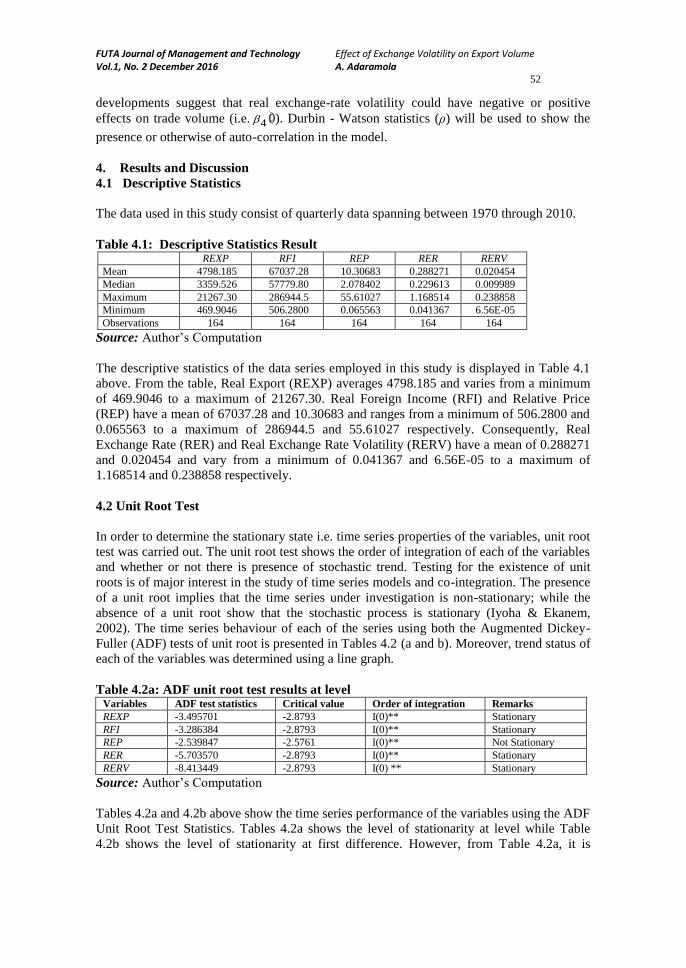
Table 4.1: Descriptive Statistics Result REXP RFI REP RER RERV
Mean 4798.185 67037.28 10.30683 0.288271 0.020454
Median 3359.526 57779.80 2.078402 0.229613 0.009989
Maximum 21267.30 286944.5 55.61027 1.168514 0.238858
Minimum 469.9046 506.2800 0.065563 0.041367 6.56E-05
Observations 164 164 164 164 164
Source: Author’s Computation
The descriptive statistics of the data series employed in this study is displayed in Table 4.1
above. From the table, Real Export (REXP) averages 4798.185 and varies from a minimum
of 469.9046 to a maximum of 21267.30. Real Foreign Income (RFI) and Relative Price
(REP) have a mean of 67037.28 and 10.30683 and ranges from a minimum of 506.2800 and
0.065563 to a maximum of 286944.5 and 55.61027 respectively. Consequently, Real
Exchange Rate (RER) and Real Exchange Rate Volatility (RERV) have a mean of 0.288271
and 0.020454 and vary from a minimum of 0.041367 and 6.56E-05 to a maximum of
1.168514 and 0.238858 respectively.
4.2 Unit Root Test
In order to determine the stationary state i.e. time series properties of the variables, unit root
test was carried out. The unit root test shows the order of integration of each of the variables
and whether or not there is presence of stochastic trend. Testing for the existence of unit
roots is of major interest in the study of time series models and co-integration. The presence
of a unit root implies that the time series under investigation is non-stationary; while the
absence of a unit root show that the stochastic process is stationary (Iyoha & Ekanem,
2002). The time series behaviour of each of the series using both the Augmented Dickey-
Fuller (ADF) tests of unit root is presented in Tables 4.2 (a and b). Moreover, trend status of
each of the variables was determined using a line graph.
Table 4.2a: ADF unit root test results at level Variables ADF test statistics Critical value Order of integration Remarks
REXP -3.495701 -2.8793 I(0)** Stationary
RFI -3.286384 -2.8793 I(0)** Stationary
REP -2.539847 -2.5761 I(0)** Not Stationary
RER -5.703570 -2.8793 I(0)** Stationary
RERV -8.413449 -2.8793 I(0) ** Stationary
Source: Author’s Computation
Tables 4.2a and 4.2b above show the time series performance of the variables using the ADF
Unit Root Test Statistics. Tables 4.2a shows the level of stationarity at level while Table
4.2b shows the level of stationarity at first difference. However, from Table 4.2a, it is
FUTA Journal of Management and Technology Effect of Exchange Volatility on Export Volume Vol.1, No. 2 December 2016 A. Adaramola
53
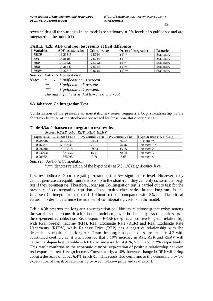
revealed that all the variables in the model are stationary at 5% levels of significance and are
integrated of the order I(1).
TABLE 4.2b: ADF unit root test results at first difference Variables ADF test statistics Critical value Order of integration Remarks
REXP -16.23815 -2.8794 I(1)** Stationary
RFI -17.56194 -2.8794 I(1)** Stationary
REP -17.19629 -2.5762 I(1)* Stationary
RER -17.26448 -2.8794 I(1)** Stationary
RERV -17.32816 -2.8794 I(1) ** Stationary
Source: Author’s Computation
Note: * - Significant at 10 percent
** - Significant at 5 percent
*** - Significant at 1 percent;
The null hypothesis is that there is a unit root.
4.3 Johansen Co-integration Test
Confirmation of the presence of non-stationary series suggests a bogus relationship in the
short-run because of the stochastic possessed by these non-stationary series.
Table 4.3a: Johansen co-integration test results
Series: REXP RFI REP RER RERV Eigen value Likelihood Ratio 5% Critical Value 1% Critical Value Hypothesized No. of CE(s)
0.595680 200.3943 68.52 76.07 None **
0.169871 53.69531 47.21 54.46 At most 1 *
0.092386 23.53518 29.68 35.65 At most 2
0.037936 7.831456 15.41 20.04 At most 3
0.009621 1.566205 3.76 6.65 At most 4
Source: Author’s Computation
*(**) denotes rejection of the hypothesis at 5% (1%) significance level
L.R. test indicates 2 co-integrating equation(s) at 5% significance level. However, they
cannot generate an equilibrium relationship in the short-run; they can only do so in the long-
run if they co-integrate. Therefore, Johansen Co-integration test is carried out to test for the
presence of co-integrating equation of the multivariate series in the long-run. In the
Johansen Co-integration test, the Likelihood ratio is compared with 5% and 1% critical
values in order to determine the number of co-integrating vectors in the model.
Table 4.3b presents the long-run co-integration equilibrium relationship that exists among
the variables under consideration in the model employed in this study. As the table shows,
the dependent variable, (i.e. Real Export - REXP), depicts a positive long-run relationship
with Real Foreign Income (RFI), Real Exchange Rate (RER) and Real Exchange Rate
Uncertainty (RERV) while Relative Price (REP) has a negative relationship with the
dependent variable in the long-run. From the long-run equation as presented in 4.3 with
substituted coefficients, it was observed that a 10% increase in RFI, RER and RERV will
cause the dependent variable – REXP to increase by 9.9 %, 9.6% and 7.2% respectively.
This result conforms to the economic a priori expectation of positive relationship between
real export and real foreign income. Consequently, a 10% increase change in REP will bring
about a decrease of about 6.4% in REXP. This result also conforms to the economic a priori
expectation of negative relationship between relative price and real export.
FUTA Journal of Management and Technology Effect of Exchange Volatility on Export Volume Vol.1, No. 2 December 2016 A. Adaramola
54
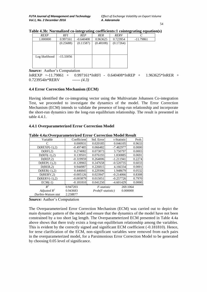
Table 4.3b: Normalized co-integrating coefficients:1 cointegrating equation(s) REXP RFI REP RER RERV C
1.000000 0.997161 -0.640408 0.963625 0.723954 -11.79861
(0.25688) (0.11587) (0.48108) (0.17264)
Log likelihood -15.33056
Source: Author’s Computation
lnREXP =-11.79861 + 0.997161*lnRFI - 0.640408*lnREP + 1.963625*lnRER +
0.723954ln*RERV ------ (4.3)
4.4 Error Correction Mechanism (ECM)
Having identified the co-integrating vector using the Multivariate Johansen Co-integration
Test, we proceeded to investigate the dynamics of the model. The Error Correction
Mechanism (ECM) intends to validate the presence of long-run relationship and incorporate
the short-run dynamics into the long-run equilibrium relationship. The result is presented in
table 4.4.1.
4.4.1 Overparameterized Error Correction Model
Table 4.4a:Overparameterized Error Correction Model Result Variable Coefficient Std. Error t-Statistic Prob.
C 0.000931 0.020185 0.046105 0.9633
D(REXP(-1),2) -0.497485 0.066482 -7.482977 0.0000
D(RFI,2) 0.274082 0.073073 3.750797 0.0003
D(RFI(-1),2) 0.139501 0.076193 1.830885 0.0691
D(REP,2) -0.319959 0.264006 -1.211941 0.2274
D(REP(-1),2) -0.128965 0.247658 -0.520735 0.6033
D(RER,2) 0.944987 0.226815 4.166334 0.0001
D(RER(-1),2) 0.446845 0.229306 1.948679 0.0532
D(RERV,2) -0.005126 0.023947 -0.214066 0.8308
D(RERV(-1),2) -0.003879 0.015051 -0.257726 0.7970
ECM(-1) -0.181810 0.041250 -4.601429 0.0000
R2 0.947203 F-statistic 269.1064
Adjusted R2 0.943683 Prob(F-statistic) 0.000000
Durbin-Watson stat 2.258877
Source: Author’s Computation
The Overparameterized Error Correction Mechanism (ECM) was carried out to depict the
main dynamic pattern of the model and ensure that the dynamics of the model have not been
constrained by a too short lag length. The Overparameterized ECM presented in Table 4.4a
above shows that there truly exists a long-run equilibrium relationship among the variables.
This is evident by the correctly signed and significant ECM coefficient (-0.181810). Hence,
for terse clarification of the ECM, non-significant variables were removed from each pairs
in the overparameterized model, for a Parsimonious Error Correction Model to be generated
by choosing 0.05 level of significance.
FUTA Journal of Management and Technology Effect of Exchange Volatility on Export Volume Vol.1, No. 2 December 2016 A. Adaramola
55
4.4.2 Parsimonious Error Correction Model
The Parsimonious ECM result presented in Table 4.4b above shows that the coefficient of
one period lag of ECM is statistically significant and correctly signed. This validates the
existence of long-run equilibrium relationship among the variables despite the presence of
short-run inconsistencies due to non-stationary of one of the series.
Table 4.4b: Parsimonious Error Correction Model Result Variable Coefficient Std. Error t-Statistic Prob.
C 0.000976 0.020052 0.048662 0.9613
D(REXP(-1),2) -0.498655 0.065185 -7.649862 0.0000
D(RFI,2) 0.263775 0.071870 3.670166 0.0003
D(RFI(-1),2) 0.135157 0.074021 1.825931 0.0698
D(RER,2) 0.661871 0.064924 10.19453 0.0000
D(RER(-1),2) 0.331054 0.078571 4.213418 0.0000
ECM(-1) -0.193805 0.040789 -4.751405 0.0000
R2 0.946499 F-statistic 454.0763
Adjusted R2 0.944415 Prob(F-statistic) 0.000000
Durbin-Watson stat 2.256991
Source: Author’s Computation
D(REXP,2) = 0.0009757852388 – 0.498655356*D(REXP(-1),2)+0.2637749787*D(RFI,2) +
0.1351572058*D(RFI(-1),2) + 0.6618713705*D(RER,2) + 0.3310541545*D(RER(-1),2) -
0.1938045609*ECM(-1) --------------------- (4.4)
The result shows that about 19% of the short-run inconsistencies are being corrected and
incorporated into the long-run equilibrium relationship. In the parsimonious ECM result, the
short-run inter-relationship between differenced real foreign income and real export is
positive and statistically significant. The significance of the coefficient can be attributed to
fact that an increased foreign income (foreign exchange earnings) will boost the productive
capacity of the economy thereby leading to increased export of domestic goods. This result
however conforms to the economic a priori expectation of positive relationship. However, a
10% increase real foreign income will bring about 2.6% increase in real export in the short-
run. Consequently, from the parsimonious ECM result presented in the Table 4.4b, it is
observed that real exchange rate depicts a positive and statistically significant relationship
with the explained variables – real export. This result however does not conform to the
economic a priori expectation of negative relationship with the explained variable. This is
due to the ever increasing exchange Nigeria exchange rate at the international market.
However, since crude oil provides the major export earnings of the economy, and this
commodity is indispensable to by the Nigeria’s importing trade partners, the increasing
exchange rate will further increase export as a result of the adduced reason, hence, a unit
change in the real exchange rate will bring about an increase of about 0.6% in the value of
real export in the economy. Moreover, the result shows the coefficient of multiple
determination (R2) to be 0.946499. This implies that 95% of the systematic variations in the
dependent variable (real export) can be explained by the explanatory variables. Moreover,
the statistical significance of the F-Statistics depicts the overall goodness of fit of the model.
This implies that the systematic variations in the dependent variable are truly explained by
the behaviour of the explanatory variables. However, the Durbin Watson test of first order
serial autocorrelation is inconclusive.

FUTA Journal of Management and Technology Effect of Exchange Volatility on Export Volume Vol.1, No. 2 December 2016 A. Adaramola
56
4.5 ARCH and GARCH Model
This section aims to test for the presence of volatility by employing the ARCH and GARCH
model.
4.5.1 Mean Equation
eRFIφRER = φ 21 --------------------- (4.5)
where
RER= Real rate of exchange,
RFI= Real foreign income accruing from transactions in the international market,
e = Residual.
Having estimated the OLS regression of the above mean equation model, the residual plot
result for ascertaining the presence/absence of ARCH and GARCH effect is presented in the
figure below;
Figure 4.1: Residuals of Nigeria Exchange Rate
Source: Author’s Computation
It is evident from Figure 4.1 that there is prolonged period of low volatility from 1970 to
1974 and a prolonged period of high volatility from 1975 to 1980. In other words, periods of
low volatility are followed by periods of high volatility and period of high volatility are
followed by periods of low volatility. This suggests that the residual or error term is
heteroscedastic and it can be represented by ARCH and GARCH model.
4.5.2 Variance Equation
Residuals derived from the mean equation above is used in making the variance equation,
this is presented below;
OPeHt
t 62
5143t1
= H
--------------------- (4.6)
where:
Ht= variance of the residual (error term) derived from the mean equation. It is also
known as the current year’s volatility of Nigeria exchange rate in real term.
5 = constant
Ht-1 = previous year’s residual variance of Nigeria’s real exchange rate. It is also known
as the GARCH term
-6,000
-4,000
-2,000
0
2,000
4,000
6,0000
5,000
10,000
15,000
20,000
25,000
1970 1975 1980 1985 1990 1995 2000 2005 2010
Residual Actual Fitted
FUTA Journal of Management and Technology Effect of Exchange Volatility on Export Volume Vol.1, No. 2 December 2016 A. Adaramola
57
2
1te = previous period’s squared residual derived from the mean equation. It is also
previous year’s real exchange rate information about volatility. This is the ARCH
term.
OP= Oil price in the international market. It is an exogenous or predetermined variable.
Equation (4.6) is a GARCH (1.1) model as it has one ARCH (2
1te ) and one GARCH (Ht-1)
term. In other words, it refers to a first order ARCH term and a first order GARCH term.
Hence, the mean equation of equation (4.5) as well as the variance equation of equation
(4.6) shall be estimated thus simultaneously. It should however be noted that this study aims
to model the volatility of Nigeria real exchange rate and the factor(s) affecting the volatility
of Nigeria real exchange rate.
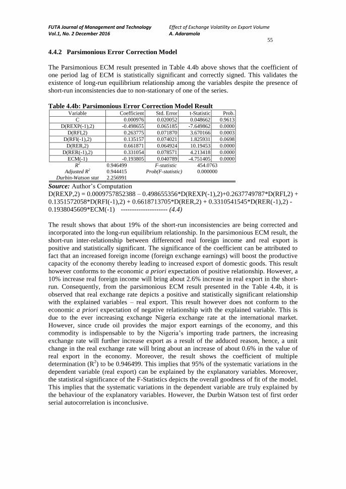
4.5.3 Result and Discussion of GARCH (1.1) Model: Variance Equation
Annual data for estimating GARCH (1.1) model have been chosen in which all the variables
therein are assumes to be stationary. However, the student’s t-distributions have been
employed in this analysis.
Table 4.5: Result of GARCH (1.1) Model
Dependent Variable: RER Method: ML - ARCH (Marquardt) - Student's t distribution
GARCH = C(3) + C(4)*RESID(-1)^2 + C(5)*GARCH(-1) + C(6)*OP
Variable Coefficient Std. Error z-Statistic Prob.
C 0.165123 0.015311 10.78487 0.0000
RFI 3.57E-07 1.25E-07 2.855856 0.0043
Variance Equation
C 0.003273 0.001459 2.243728 0.0248
RESID(-1)^2 0.336939 0.154953 2.174451 0.0297
GARCH(-1) 0.568444 0.164497 3.455649 0.0005
OP -0.000111 3.22E-05 -3.458511 0.0005
Source: Author’s Computation
Under this distribution as presented in Table 4.5, ARCH is significant. This implies that the
previous year’s real exchange rate information (that is, 2
1te in equation 4.6) can influence this
year’s real exchange rate volatility (that is, Ht in equation 4.6). In the same vein, under this
distribution, GARCH is also significant. This means that the previous year’s real exchange
rate volatility (that is, Ht-1in equation 4.6) can influence this year’s real exchange rate
volatility. This result implies that Nigeria’s real exchange rate is influenced by its own
ARCH and GARCH factors or own shocks. On the other hand, Oil Price (OP) is significant,
meaning that the volatility in the price of oil can transmit to the exchange rate situation in
Nigeria. Therefore, we can conclude that the volatility in Nigeria exchange rate is largely
dependent on its own shocks such as ARCH and GARCH and oil price.
However, in order to ascertain if the estimated GARCH (1.1) model above is theoretically
meaningful; some of the following assumptions must be fulfilled:
i. There is no serial correlation in the residual or error term;
ii. Residuals are normally distributed; and
iii. There is no ARCH effect.
FUTA Journal of Management and Technology Effect of Exchange Volatility on Export Volume Vol.1, No. 2 December 2016 A. Adaramola
58
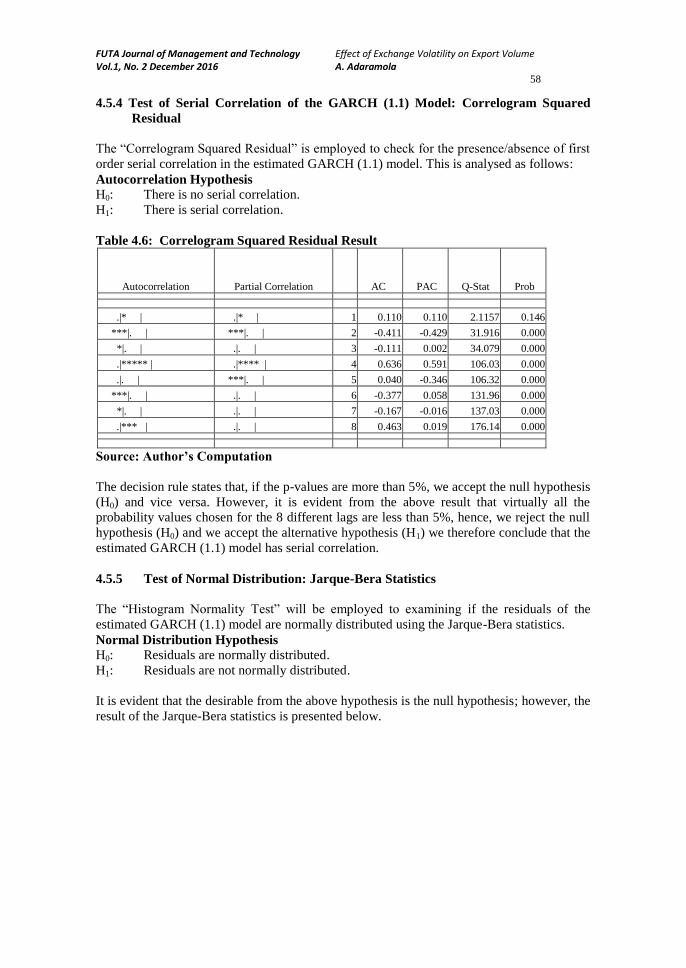
4.5.4 Test of Serial Correlation of the GARCH (1.1) Model: Correlogram Squared
Residual
The “Correlogram Squared Residual” is employed to check for the presence/absence of first
order serial correlation in the estimated GARCH (1.1) model. This is analysed as follows:
Autocorrelation Hypothesis
H0: There is no serial correlation.
H1: There is serial correlation.
Table 4.6: Correlogram Squared Residual Result
Autocorrelation Partial Correlation AC PAC Q-Stat Prob
.|* | .|* | 1 0.110 0.110 2.1157 0.146
***|. | ***|. | 2 -0.411 -0.429 31.916 0.000
*|. | .|. | 3 -0.111 0.002 34.079 0.000
.|***** | .|**** | 4 0.636 0.591 106.03 0.000
.|. | ***|. | 5 0.040 -0.346 106.32 0.000
***|. | .|. | 6 -0.377 0.058 131.96 0.000
*|. | .|. | 7 -0.167 -0.016 137.03 0.000
.|*** | .|. | 8 0.463 0.019 176.14 0.000
Source: Author’s Computation
The decision rule states that, if the p-values are more than 5%, we accept the null hypothesis
(H0) and vice versa. However, it is evident from the above result that virtually all the
probability values chosen for the 8 different lags are less than 5%, hence, we reject the null
hypothesis (H0) and we accept the alternative hypothesis (H1) we therefore conclude that the
estimated GARCH (1.1) model has serial correlation.
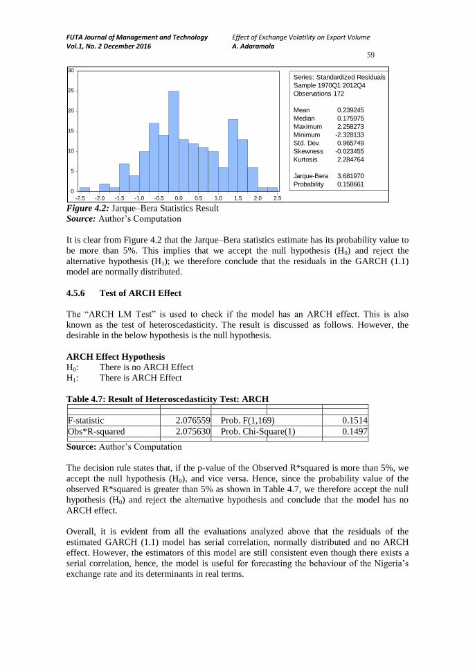
4.5.5 Test of Normal Distribution: Jarque-Bera Statistics
The “Histogram Normality Test” will be employed to examining if the residuals of the
estimated GARCH (1.1) model are normally distributed using the Jarque-Bera statistics.
Normal Distribution Hypothesis
H0: Residuals are normally distributed.
H1: Residuals are not normally distributed.
It is evident that the desirable from the above hypothesis is the null hypothesis; however, the
result of the Jarque-Bera statistics is presented below.
FUTA Journal of Management and Technology Effect of Exchange Volatility on Export Volume Vol.1, No. 2 December 2016 A. Adaramola
59
Figure 4.2: Jarque–Bera Statistics Result
Source: Author’s Computation
It is clear from Figure 4.2 that the Jarque–Bera statistics estimate has its probability value to
be more than 5%. This implies that we accept the null hypothesis (H0) and reject the
alternative hypothesis (H1); we therefore conclude that the residuals in the GARCH (1.1)
model are normally distributed.
4.5.6 Test of ARCH Effect
The “ARCH LM Test” is used to check if the model has an ARCH effect. This is also
known as the test of heteroscedasticity. The result is discussed as follows. However, the
desirable in the below hypothesis is the null hypothesis.
ARCH Effect Hypothesis
H0: There is no ARCH Effect
H1: There is ARCH Effect
Table 4.7: Result of Heteroscedasticity Test: ARCH
F-statistic 2.076559 Prob. F(1,169) 0.1514
Obs*R-squared 2.075630 Prob. Chi-Square(1) 0.1497
Source: Author’s Computation
The decision rule states that, if the p-value of the Observed R*squared is more than 5%, we
accept the null hypothesis (H0), and vice versa. Hence, since the probability value of the
observed R*squared is greater than 5% as shown in Table 4.7, we therefore accept the null
hypothesis (H0) and reject the alternative hypothesis and conclude that the model has no
ARCH effect.
Overall, it is evident from all the evaluations analyzed above that the residuals of the
estimated GARCH (1.1) model has serial correlation, normally distributed and no ARCH
effect. However, the estimators of this model are still consistent even though there exists a
serial correlation, hence, the model is useful for forecasting the behaviour of the Nigeria’s
exchange rate and its determinants in real terms.
0
5
10
15
20
25
30
-2.5 -2.0 -1.5 -1.0 -0.5 0.0 0.5 1.0 1.5 2.0 2.5
Series: Standardized Residuals
Sample 1970Q1 2012Q4
Observations 172
Mean 0.239245
Median 0.175975
Maximum 2.258273
Minimum -2.328133
Std. Dev. 0.965749
Skewness -0.023455
Kurtosis 2.284764
Jarque-Bera 3.681970
Probability 0.158661

FUTA Journal of Management and Technology Effect of Exchange Volatility on Export Volume Vol.1, No. 2 December 2016 A. Adaramola
60
5 Conclusion and Recommendations
The effect of real exchange rate volatility on real exports as estimated in this paper suggests
that risk-averse exporters will reduce their activities, switch sources of supply and demand or
change prices in order to minimize their exposure to the effect of exchange risk. This, in turn,
can alter the distribution of output across many sectors in the Nigerian economy. A major
policy lesson of this finding is that trade policy actions aimed at stabilizing the export market
are likely to generate uncertain results at best, if policymakers ignore the stability, as well as
the level, of the real exchange rate. Another implication is that trade adjustment programmes
in Nigeria that have mostly stressed the need for export expansion may lose their appeal to
local policymakers in periods of high exchange rate volatility. Also, the intended positive
effect of a trade liberalization policy may not only be doomed by a variable exchange rate but
could also precipitate a balance-of-payments crisis. This study concludes that real exchange
rate uncertainty has significant impact on the volume of trade of the Nigerian economy. It is
therefore recommended that the monetary authorities in Nigeria should initiate policies and
programme that will stabilize naira exchange rate and remove the negative effect of exchange
rate fluctuations on Nigeria’s export performance. In addition, Nigerian exporters should take
advantage of the future market and hedge the export income (real foreign income), reducing
the effect of exchange rate fluctuations on export trade. Since interest rate fluctuation is a
function of import which itself is a reflection of the poor industrial base of the nation,
affecting export capacity, the Nigerian government should initiate policies to boost local
production to satisfy local consumption, reduce demand and pressure on the naira exchange
rate, stabilize the rate while increasing production capacity, boosting stock of export goods,
growth and income.
References Adubi, A. A., & Okumadewa, F. (1999). Price exchange rate volatility and Nigeria’s trade flows: a dynamic
analysis. AERC Research paper 87. Nairobi: African Economic Research Consortium.
Aliyu, S. U. R. (2009). Impact of oil price shock and exchange rate volatility on economic growth in Nigeria: An empirical investigation. Research Journal of International Studies, 11.
Anderton, R., & Skudelny, F. (2001). Exchange rate volatility and euro area imports. European Central Bank
(ECB) Working Paper, No. 64. Barkoulas, J., Baum, C., & Caglayan, M. (2002). Exchange rate effects on the volume and variability of trade
flows. Journal of International Money and Finance, 21(4), 481-496.
Blonigen, B.A., & Piger, J. (2011).Determinants of foreign direct investment. NBER Working Paper 16704. Breuer, J. B., & Leianne, A. C. (2003).The commodity composition of US-Japanese trade and the yen/dollar real
exchange rate. Japan and the World Economy, 15(3), 307-330.
Callabero, R., & Corbo, V. (1989). The effect of real exchange rate uncertainty on exports: Empirical evidence. The World Bank Economic Review, 3(2), 263-278.
CBN Statistical Bulletin (2010)
Chinn, M. (1997). Sectoral productivity, government spending, and real exchange rates: Empirical evidence for OECD countries. NBER Working Paper Series 6017.
Chinn, M., & Johnston, L. (1999).The impact of productivity differentials on real exchange rates: Beyond the
Balassa-Samuelson framework, (Working Paper 442). Santa Cruz: University of California Dept. of Economics.
Chukwu, (2007). Exchange rate fluctuation and export performance in Nigeria (1961-2011). Unpublished Undergraduate Project.
Clark, P. B. (1973). Uncertainty, exchange risk, and the level of international trade. Western Economic Journal,
11(3), 302-313. Clark, P., Tamirisa, N., & Wei, S. J. (2004).Exchange rate volatility and trade flows-some new evidence. IMF
Working Paper, May 2004, International Monetary Fund.
Cui, L., & Syed, M. (2007).The shifting structure of china's external trade and its implications. Forthcoming IMF Working Paper (Washington: International Monetary Fund).
De Grauwe, P. (1988). Exchange rate variability and the slowdown in the growth of international trade. IMF Staff
Papers, 35(1): 63-84.

FUTA Journal of Management and Technology Effect of Exchange Volatility on Export Volume Vol.1, No. 2 December 2016 A. Adaramola
61
Egert, B, & Morales, Z. (2005). Exchange rate regimes, foreign exchange volatility, and export performance in
Central and Eastern Europe: Just another blur project? William Davidson Institute Working Paper Number 782.
Emilio J. Medina-Smith (2001). Is the export-led growth hypothesis valid for developing countries? A case study of
Costa Rica. Policy Issues in International Trade and Commodities, Study series No. 7 United Nations, New York and Geneva, 2001.
Froot, K. A., & Stein, J. C. (1991) Exchange rates and foreign direct investment: An imperfect capital markets
approach. The Quarterly Journal of Economics, 106(4), 1191-1217. Ghura, D., & Greenes, T. J. (1993). Gauging exchange rate volatility on the trade flows of sub-Saharan Africa
countries. Journal of Development Economics, 42(32), 155-174.
Gibson, L., & Ward, M. D. (1992). Export orientation: Pathway or artifact? International Studies Quarterly, 36(3), 331-343.
Goldstein, J., & Pevehouse, C. (2008).International relations (8thed.). New York: Pearson Longman.
Hartman, R. (1972). The effects of price and cost uncertainty on investment. Journal of Economic Theory, 5(2), 258-266
Hooper, P., & Kohlhagen, S. (1978). The effect of exchange rate uncertainty on the prices and volume of
international trade. Journal of International Economics, 8(4), 483-511. Ihimodu, I. I. (1993). The Structural Adjustment Programme and Nigeria’s agricultural development (NCEMA
Monograph Series, No. 2). Ibadan: National Centre for Economic Management and Administration
(NCEMA). IMF Staff Country Report 02/170 (Ireland) – accessible here:
https://www.imf.org/external/pubs/cat/longres.aspx?sk=16007.0
Iyoha, A. M., & Oriakhi, D. (2002).Explaining African economic growth performance: the case of Nigeria. Report on Nigerian case study prepared for AERC project on “Explaining African Economic growth
performance”.
Johansen (1988), Statistical nalysis of Co-integrations Vectors, Journal of Economics Dynamics and Control, 12, 231-254
Lama, R., & Medina, J. P. (2010). Is exchange rate stabilization an appropriate cure for the Dutch disease? (IMF working paper No 182). Retrieved from www.imf.org on 2/2/ 2010.
McCombie, J. S. L., & Thirlwall, A. P. (1994). Economic growth and the balance-of-payments constraint. New
York: St. Martin's. McKenzie, M. D. (1999).The impact of exchange rate volatility on international trade flows. Journal of Economic
Surveys, 13(1), 71-106.
Obadan, M. I. (2006). Overview of exchange rate management in Nigeria from 1986 to date, In the Dynamics of Exchange Rate in Nigeria. Central Bank of Nigeria Bullion, 30(3), 1-9.
Oguro, Y., Fukao, K., & Khatri, Y. (2008).Trade sensitivity to exchange rates in the context of intra-industry trade.
(IMF Working Paper WP/08/134). Retrieved from www.imf.org. Osuntogun, A., Edordu, C. C., & Oramah, B. O. (1993).Promoting Nigeria’s non-oil export: an analysis of some
strategic issues. Nairobi: African Economic Research Consortium.
Oyejide, T. A. (1986). The effect of trade and exchange rate policies on agriculture in Nigeria. Research report 55, Washington, D. C.: International Food Policy Research Institute.
Samanta, S. (1998). Exchange rate uncertainty and foreign trade for a developing country: An empirical analysis.
The Indian Economic Journal, 45(8), 51-65. Srour, G. (2006). The implications of trade barriers for sectoral diversification and macroeconomic stability in
developing economies, (IMF working paper N0. 50). Retrieved from www.imf.org on 8/9/2007.
Thorbecke, W. (2006).The effect of exchange rate changes on trade in East Asia. Discussion paper 06009, Research Institute of Economy, Trade and Industry (RIETI).
Walsh, J. P., & Yu, J. (2010). Determinants of foreign direct investment: A sectoral and institutional approach.
(IMF Working Paper WP/10/187) Asian Pacific Department. World Trade Organization (2010). 10 benefits of the WTO trading system. Retrieved from http://www.wto.org/
trade policy/country/Nigeria.