Exchange Rate Volatility and Export Growth in South …2015.essa.org.za/fullpaper/essa_3190.pdf · Exchange Rate Volatility and Export Growth in South Africa: ... Section 3 presents

1

Exchange Rate Volatility and Export Growth in South Africa: An ARDL Bounds Testing Approach

Author:

Azwifaneli Innocentia (Mulaudzi) Nemushungwa

Email:[email protected]

Pomotors:

Prof. Agyapong Gyekye

Email:[email protected]

Prof. Matthew, K. Ocran

Email:[email protected]

Abstract

The adoption of the flexible exchange rate system in 1973 resulted in significant volatility and uncertainty in

exchange rates. Likewise, since its adoption of flexible exchange rates system in the mid 1990’s, the South

African rand has been very volatile. The requirement by South African government to promote exports in an

environment of a flexible exchange rate requires a comprehensive understanding of how the highly fluctuating

rand impacts on the South Africa exports and the resultant effects on the economy at large. Against this

backdrop, this chapter empirically investigates the impact of exchange rate volatility on South African exports

using the ARDL bounds testing procedure and monthly data for the period 2000 to 2013.Furthermore; it

measures real exchange rate volatility and also examines the stability of the long run coefficients and the short-

run dynamics. The study results confirm that exchange rate volatility has insignificant negative long run impact

on South African exports. Besides, real exchange rate has insignificant negative long-run effects on South African

exports. The coefficient of error correction term for exports model, is positive and statistically insignificant and is

therefore not supportive of the validity of the long-run equilibrium relationship between the variables.

Key words: real exchange rate volatility, ARDL bounds testing procedure, short run dynamics and structural

breaks.

2

1. Introduction

1.1. Background

The trade liberalization programme pursued by South Africa since 1994 has resulted in a much

more open economy. Between 1994 and 2002, import penetration and export orientation ratios

rose in all 28 sectors of the standard industrial classification where in ten of these sectors, export

orientation increased by more than double. In 2007, total exports and imports of goods and

services amounted to 31 per cent and 35 per cent of GDP, respectively. The increase in export

values was due to high gold and platinum prices and a weaker rand. Mining products, such as

platinum, iron and coal, benefited from high demand from Asian countries. Exports of some

manufactured goods, particularly automobiles, chemicals and mining machinery also increased.

However, the current account balance had progressively deteriorated since 2003, reflecting a

widening trade deficit (Economic Outlook, 2008).

During fourth quarter of 2012 mining output fell by 6.1 percent (relative to the third quarter) due

to industrial action related production stoppages that started in the third quarter of 2012. Gold,

iron ore and platinum production contracted by 26.3 per cent, 17.3 per cent and 4.2 per cent,

respectively. In contrast, coal and diamond output increased by 3.2 per cent and 38.3 per cent

respectively. Overall, mining output fell by 3.1 per cent in 2012. Consequently, commodity

exports were severely affected, particularly in case of platinum and gold. In contrast, exports of

chemical products and transport equipment (especially vehicles) rose strongly, though only a

slight increase in unit terms occurred(Economic Overview, 2013)..

The poor export performance of the mining industry and certain sub-sectors of manufacturing

was clearly reflected in the substantial deterioration of South Africa’s trade balance, as overall

exports grew by a mere 0.8 percent in nominal value terms in 2012, against a 14.6 percent

growth in import demand. A widening trade deficit of R117.7 billion occurred, relative to a

much smaller R16.9 billion deficit in 2011 (Economic Overview, 2013).

Economic overview

In the first 11 months of 2013, exports rose to the value of R846 billion over R817 billion in

2012, boosted by the rand’s deterioration, while imports increased to R921 billion up from R852

billion. As a result the trade deficit almost doubled, rising from R40 billion in 2012 to over R74

billion in 2013 (African Economic Outlook, 2014).

3

1.2. Problem Statement

The adoption of the flexible exchange rate system in 1973 resulted in significant volatility and

uncertainty in exchange rates (Vergi,2002).The birth of this new system of exchange rate has

also prompted a ‘hot’ and extensive theoretical debate regarding the impact of exchange rate

variability on foreign trade (Johnson, 1969; Kihangire, 2004). However, both the theoretical and

empirical studies yielded conflicting results about the relationship between exchange rate

variability and international trade flows (Sekantsi, 2007).

Most models of trade argue that exchange rate volatility increases uncertainty and risk and

therefore hinders the trade flows. Amongst other are those by Doroodian (1999), Krugman

(1989), Hooper & Kohlhagen (1978) and Clark (1973). In contrast, other studies suggest

otherwise. Among them are studies by De Grauwe (1988); Asseery & Peel (1991) and

Chowdhury (1993).

As an open and middle income country in Sub-Saharan Africa (SSA), South Africa has not

escaped this debate. Ever since its adoption of flexible exchange rates system in the mid 1990’s,

the South African rand has been very volatile. The country has witnessed consistent depreciation

of exchange rate and a sharp appreciation thereafter, subjecting South African importers and

exporters to uncertainty regarding their payments and receipts in home currency terms ( Sekantsi,

2007).The requirement by South African government to promote exports in an environment of a

flexible exchange rate requires a comprehensive understanding of how the highly fluctuating

rand impacts on the South Africa exports and the resultant effects on the economy at large

(Aziakpono, et al, 2005; Todani & Munyama, 2005 and Sekantsi, 2007).

Against this background, this chapter analyzes the impact of rand volatility on South African

exports. It furthermore determines the long run relationships among the variables and estimates

the coefficients of the long and short run relationships and also determines the magnitude as well

as the speed of adjustment among the variables being modelled. The present study will cover the

period during the Eurozone crisis, which the studies by Aziakpono, et al, 2005; Todani &

Munyama, 2005 and Sekantsi (2007) did not cover. This will therefore help to ascertain the

existence of structural breaks during this period.

4

The chapter is organized as follows: Section 4.2 reviews the literature on exports and exchange

rate volatility. The outline of theoretical and empirical review is discussed in sections 2.1 and 2.2

respectively. Section 3 presents theoretical framework and model specification. Section 4

presents data issues. In sections 5 and 6, estimation techniques and the empirical results are

presented respectively. Section 7 presents conclusion and suggestions for policy interventions.

2. Review of the Literature

2.1. Theoretical Literature Review

There are several theories in economic literature that are used to assess the effect of

depreciation/devaluation on trade balance. Amongst them are the elasticity approach, monetary

approach, absorption approach and the gravity equation approach.

The elasticity approach, propounded by Robinson (1947) and Metzler (1948) and popularized by

Kreuger (1983), states that transactions under contract completed during the period of

devaluation/ depreciation may affect the trade balance negatively in the short run. However, over

time, export and import quantities adjust, which give rise to increase in exports and imports

elasticities and adjustment in quantities. Consequently, the foreign price of the

devaluing/depreciating country's export is reduced and the price of imported goods is increased,

which directly reduces the demand for imports at the long run the trade balance improves. This

theory clearly states that the effect of devaluation/depreciation is dependent on the elasticity of

exports and imports.

The elasticity approach, commonly known as the BRM model (after the proponents Bickerdike,

1920; Robinson, 1947; Metzler, 1948), has been recognized in the literature as providing a

sufficient condition for a trade balance improvement when exchange rates devalue/depreciate.

The monetary approach stresses that balance of payment is a monetary phenomenon (Frenkel

and Johnson 1977). The monetarist view is based on the argument that devaluation/depreciation

reduces the real value of cash balances and changes in relative price of traded and non-traded

goods, and causes the trade balance to improve (Miles, 1979). However, higher import prices

that will arise due to devaluation/depreciation may contribute to higher overall domestic prices

5

of non-traded goods and then impact negatively on the trade balance (Williams 1983, Upadyaya

and Dhakal, 2003; Hernan, 1998).

The gravity equation model, introduced by Cameron, Kihangire and Potts (2001), estimated the

bilateral trade flows between countries as depending positively on the product of their GDP’s

and negatively related to their geographical distance from each other.

The Constant Market Share (CMS) analysis developed by Tyszynski (1951) and later refined by

Milana (1988). The model involves decomposition of an identity (Ahmadi-Esfahani, 2006). It

measures a country’s share of world exports in a particular commodity or other export items. It is

based on the assumption that an industry should maintain its export share in a given market (i.e.

remain unchanged over time). If a country’s share of total products exports is growing in relation

to competitors, for example, this may reflect increasing competitiveness of that country’s product

sector (Siggel, 2006).

Another approach is to estimate a simple export demand equation with real exports as a

dependent variable and exchange rate volatility together with relative prices and a measure of

economic activity variable as regressors (Todani and Munyama, 2005; Goudarzi, 2012).This

study will also apply the simple export demand equation, but with nominal exports (rather than

real exports) as a dependent variable.

2.2. Empirical Literature Review

2.2.1. Introduction

Studies conducted for both developed and developing countries present contradicting results on

the relationship between exchange rate volatility and exports. This study will also contribute to

the ongoing debate on this issue.

2.2.2. Literature for developed countries

De Vita and Abbott (2004) use the autoregressive distributed lag (ARDL) technique and

disaggregated monthly data for period 1993 to 2001 to analyze the impact of exchange rate

volatility on UK exports to the European Union (EU). The results show that UK export to the EU

are largely unaffected by exchange rate volatility.

6

Dell' Ariccia (1999) used the gravity model and provides a systematic analysis of exchange rate

volatility on the bilateral trade of the 15 EU members and Switzerland over a period of20 years

from 1975 to 1994. In the basic regressions, exchange rate volatility has a small but significantly

negative impact on trade.

Hooper and Kohlhagen (1978) examined the effects of exchange rate uncertainty on the volume

of trade among developed countries. They do not find any significant impact of exchange rate

volatility on the volume of trade. However, Cushman (1983) found negative relation between

exchange rate volatility and volume of trade in the developed countries.

Akhtar and Hilton (1984) examined the bilateral trade between West Germany and US and found

that the exchange rate volatility has a significant negative impact on the exports and imports of

two countries.

Bailey et al. (1986) investigated the effect of exchange rate volatility on export of leading OECD

countries (Canada, France, Germany, Italy, Japan, UK and US). The study revealed that

exchange rate volatility has positive effect both in long run and short run.

Chowdhury (1993) investigated the impact of exchange rate volatility on the trade flows of the

G-7 countries, in context of a multivariate error-correction model. They found that the exchange

rate volatility has a significant negative impact on the volume of exports in each of the G-7

countries.

Qian and Virangis (1994) examined the impact of exchange rate volatility on trade in six

countries using ARCH model. The empirical results showed a negative link between exchange

rate volatility and export volumes for Australia, Canada, and Japan and positive for United

Kingdom, Sweden, and Netherlands.

For developing countries

Tandrayen-Ragoobur and Emamdy (2011), using ARDL model, analyses the impact of real

effective exchange rate volatility on the Mauritian export performance from 1975 to 2007.

Exchange rate volatility is derived from the moving average standard deviation method since no

7

GARCH effect was obtained. Their findings reveal that exchange rate volatility has a positive

and significant short run effect on exports, whilst in the long run; volatility adversely affects the

Mauritian exports.

Umaru et al. (2013) employs the ordinary Least Square, Granger causality test, ARCH and

GARCH techniques to investigate the impact of exchange rate volatility on export in Nigeria The

study further showed that exchange rate is impacting positively on export, as shown by the

regression results. The elasticity results revealed that, the demand for Nigerian products in the

World market is fairly elastic.

Ogundipe et al (2013) investigates the impact of currency devaluation on Nigerian trade balance

using the Johansen co-integration and variance decomposition analyses for the period 1970-

2010. The empirical results indicate that there exist no short run causality from exchange rate to

trade balance and money supply volatility contributes more to variance in trade balance than

exchange rate volatility.

Omojimite and Akpokodje (2010) empirically compare the effect of exchange rate volatility on

the exports of the panel of Communaute Financiere Africaine (CFA) countries with that of the

non-CFA counterparts during the period 1986-2006. Exchange rate volatility series were

generated utilizing the GARCH model. The results reveal that the system GMM technique

performed better than the other estimation techniques. Exchange rate volatility was found to

negatively impinge on the exports of both panels of countries. However, exchange rate volatility

has a larger effect on the panel of the non-CFA countries than on the CFA.

Alege and Osabuohien (2011), using panel co-integration with the application of Granger

Causality test, investigate exchange rate-trade nexus in SSA countries. Based on partial

equilibrium analysis, they develop two equations for export and import in which exchange rate,

real GDP, stock of capital, and technology are the independent variables. It was found that export

and import are inelastic to changes in exchange rate. It follows that depreciation of currencies in

the region may not have the expected results in view of the structure of the economies and export

compositions. In the same vein, depreciation would not depress imports but only aggravate

balance of payments.

8

Chit et al. (2008), employing a generalized gravity model that combines a long run demand

model with gravity type variables, examined the impact of bilateral real exchange rate volatility

on real exports on five emerging East Asian countries. The study found strong evidence that

exchange rate volatility has a negative impact on the exports of emerging East Asian countries.

Srinivasan and Kalaivan (2013), using the ARDL bounds testing procedure proposed by Pesaran,

Shin and Smith (2001) and annual data for the period 1970 to 2011, empirically investigates the

impact of exchange rate volatility on the real exports in India. Their findings indicate that the

exchange rate volatility has significant negative impact on real exports both in the short-run and

long-run.

Fang et al (2006) investigated the effect of exchange rate movement on exports of Eight Asian

countries. The study revealed that real exchange rate depreciation has significant impact on

exports for all countries except Singapore, whereas exchange rate risk proves positive for

Malaysia and Philippines but negative for Indonesia, Japan, Singapore, Taiwan and no effect for

Korea and Thailand.

Moccero and Winograd (2007), using the ARCH/GARCH and Markov SWARCH models, they

analyzed the link between real exchange rate volatility and exports in the case of Argentina. The

study showed that decrease in real exchange volatility has an impact on exports to Brazil but a

negative impact for the rest of world.

Aliyu (2008), using the Johansen cointegration analysis examined the impact of exchange rate

volatility on non-oil export trade in Nigeria. The study observed that exchange rate volatility was

found to have an adverse effect on non-oil exports in the long-run while in the short run, there is

positive relationship.

Arize et. Al, (2000) investigates empirically the impact of real exchange-rate volatility on the

export flows of eight Latin American countries over the quarterly period 1973-1997. Estimates

of the cointegrating relations are obtained using Johansen's multivariate procedure. Estimates of

the short-run dynamics are obtained utilizing the error-correction technique. The major results

show that increases in the volatility of the real effective exchange rate, approximating exchange-

9

rate uncertainty, exert a significant negative effect upon export demand in both the short-run and

the long-run in each of the eight Latin American countries.

Hooy and Choong (2010), employing EGARCH model examined the impact of currency

volatility on export demand within SAARC region (Bangladesh, India, Pakistan and Sri Lanka).

The results showed that real exchange rate volatility had negative relationship with exports

among the SAARC counterparts. Their results show positive effects of effects on exports in

most, but not all the South Asian countries.

Hosseini and Moghaddasi (2010) used the ARDL bound testing procedures and observed that

there is no significant relationship between Iranian exports flows and exchange rate volatility.

Besides, Alam and Ahmad (2011) based on the ARDL analysis showed that real exports are

cointegrated with volatility of real effective exchange rate. The study results revealed that

volatility of real effective exchange rate adversely affects the Pakistan’s exports.

Verena and Nawsheen (2011) empirically investigated the impact of real effective exchange rate

volatility on the Mauritian export performance. The results proved that exchange rate volatility

has positive effects on exports in the short-run while in the long-run, the impact was negative.

Srinivasan and Kalaivani (2012) empirically investigates the impact of exchange rate volatility

on the real exports in India using the ARDL bounds testing procedure proposed by Pesaran et al.

(2001). Using annual time series data, the empirical analyses has been carried out for the period

1970 to 2011. Their findings indicate that the exchange rate volatility has significant negative

impact on real exports both in the short-run and long-run, implying that higher exchange rate

fluctuation tends to reduce real exports in India.

Evidence for South Africa

Poonyth & van Zyl (2000) evaluate the long run and short run effects of real exchange rate

changes on South African agricultural exports using an Error Correction Model (ECM) within

the cointegrated VAR model. The results suggest that there is a unidirectional causal flow from

exchange rate to agricultural exports. The empirical findings establish both short-run and long

run relationships between real agricultural exports and the real exchange rate.

10

Damoense and Agbola (2004) usmg the Johansen co-integration technique and VECM to

determine the lag length and also make use of the final prediction error (FPE) criteria which

indicates that domestic and foreign income, domestic money supply, domestic interest rates and

exchange rates have a negative impact on the trade balance, while foreign money supply and

interest rates have a positive impact on the trade balance.

Arize, Malindretos and Kasibhatla (2003) study a sample of 10 less developed countries (LDCs)

including South Africa. Having tested for long-run cointegration and used the error correction

technique to model the short-run dynamics of the variables, they found that exchange rate

volatility exerts a significant negative effect on export demand in both the short- and the long run

in most of the countries studied. However, South Africa was an important exception where

positive statistically significant exchange rate elasticities were obtained. These results were

qualitatively similar whether nominal or real effective exchange rates were used and when

ARCH residuals were used to measure exchange rate uncertainty.

Samson et al (2003) investigate the impact of the volatility of the exchange rate on the South

African economy. Evidence from sectoral analysis of South African manufacturing exports

documents the strong negative impact of exchange rate appreciation on the volume of exports.

Edwards and Willcox (2005) assess the impact of exchange rate movements on the South

African trade balance. In particular, they analyze whether a depreciation of the currency can

improve the trade balance through promoting export production and import substitution. The

study follows much international empirical research and uses the elasticity approach to analyze

the responsiveness of exports and imports to exchange rate movements. and draws upon the

BRM condition which defines a set of necessary conditions on the size of import demand, import

supply, export demand and export supply elasticities for a depreciation to improve the trade

balance. The study finds that export and imports remained relatively stable during the 1970s and

early 1980s, but grew strongly from the mid-1980s.

Sekantsi (2007), using GARCH and ARDL bounds testing procedure proposed by Pesaran et al.

(2001), empirically examines the impact of real exchange rate volatility on trade in the context of

South Africa’s exports to the U.S. for South Africa’s floating period (January 1995-February

11

2007) The results indicate that real exchange rate volatility exerts a significant and negative

impact on South Africa’s exports to the U.S.

Raddatz (2008) investigates the impact of exchange rate volatility on trade and exports in South

Africa using time-series and gravity equations models. The results show no evidence of a robust,

first-order detrimental effect of exchange rate volatility on aggregate exports or bilateral trade

flows.

Edwards and Garlick (2008) review the theoretical and empirical relationship between exchange

rate and trade flows in South Africa. Trade volumes are found to be sensitive to real exchange

rate movements but nominal depreciations have a limited long-run impact on trade volumes and the

trade balance, as real effects are offset by domestic inflation.

Bah and Amusi (2003) used ARCH and GARCH models to examine the effect of real exchange

rate volatility on South African exports to the U.S. for the period 1990:1- 2000:4.The findings

are that Rand’s real exchange rate variability exerts a significant and negative impact of exports

both in the long and short-run.

The similar study by Azaikpono, et al. (2005) extends the work of Bah and Amusa (2003) over

the period 1992:1-2004:4 by employing EGARCH method proposed by Nelson (1991) as a

measure of variability of exchange rate. Negative results were found.

Todani and Munyama (2005), using ARDL bounds testing procedures developed by Pesaran et al.

(2001) on quarterly data for the period 1984 to 2004, investigates the impact of exchange rate

volatility on aggregate South African exports flows to the rest of the world, as well as on South

African goods, services and gold exports. The results suggest that, depending on the measure of

volatility used, either there exist no statistically significant relationship between South African

exports flows and exchange rate volatility or when a significant relationship exists, it is positive.

Obi et al. (2013), using ARIMA/ARMA, ARCH and export demand equation, estimate the

impact of exchange rate volatility on the competitiveness of South Africa's agricultural exports to

the European Union for the period 1980-2008. The Constant Market Share model was applied to

assess the extent to which the South African citrus industry has maintained its competitive

12

advantage in several markets. The overall results strongly confirm that exchange rate volatility

has a positive impact on the competitiveness of South Africa's agricultural exports.

From the review of empirical literature on exports and exchange rate volatility, it is clear that the

findings of studies for both developed and developing countries are conflicting. Therefore, the

effect of exchange rate volatility on exports is still a debatable issue. This study will also

contribute to the ongoing debate concerning the impact of exchange rate variability on foreign

trade.

Review results also show that the ARDL approach and ARCH/GARCH model are the mostly

used methods in estimating the relationship between exchange rate volatility and export

performance. The present study will also employ the ARDL model.

3. Theoretical Framework and Model Specification

3.1 Theoretical Framework

Theoretical analyses of the relationship between higher exchange-rate volatility and international

trade transactions have been conducted by Hooper and Kohlhagen (1978), amongst others. They

argued that higher exchange-rate volatility leads to higher cost for risk-averse traders and in turn

depresses foreign trade, as the exchange rate is agreed on at the time of the trade contract, but

payment is not made until the future delivery actually takes place. If changes in exchange rates

become unpredictable this creates uncertainty about the profits to be made and, hence, reduces

the benefits of international trade. Exchange-rate risk for LDC's is generally not hedged because

forward markets are not accessible to all traders. Even if hedging in the forward markets were

possible, there are limitations and costs. For example, the size of the contracts is generally large,

the maturity is relatively short, and it is difficult to plan the magnitude and timing of all

international transactions to take advantage of the forward markets (Arize et. al,, 2000)

Conversely, recent theoretical developments suggest that there are situations in which the

volatility of exchange rates could be expected to have either negative or positive effects on trade

volume. De Grauwe (1988) stressed that the dominance of income effects over substitution

effects can lead to a positive relationship between trade and exchange-rate volatility. This is

13

because, if exporters are sufficiently risk averse, an increase in exchange-rate volatility raises the

expected marginal utility of export revenue and therefore induces them to increase exports.

Therefore, the effects of exchange-rate uncertainty on exports should depend on the degree of

risk aversion.

A traditional specification of the long-run equilibrium export demand in the flexible exchange-

rate environment is that of Arize (1995) and Chowdhury (1993),

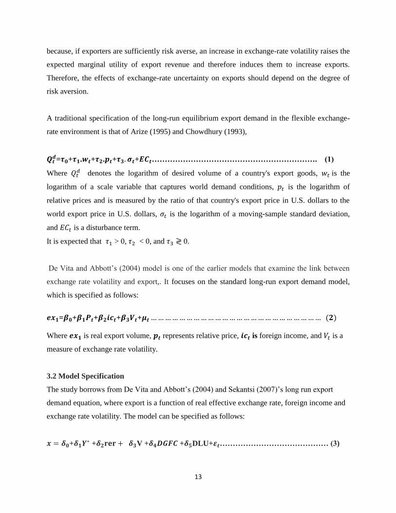
𝑸𝒕𝒅=𝝉𝟎+𝝉𝟏.𝒘𝒕+𝝉𝟐.𝒑𝒕+𝝉𝟑. 𝝈𝒕+𝑬𝑪𝒕………………………………………………………. (1)

Where 𝑄𝑡𝑑 denotes the logarithm of desired volume of a country's export goods, 𝑤𝑡 is the

logarithm of a scale variable that captures world demand conditions, 𝑝𝑡 is the logarithm of

relative prices and is measured by the ratio of that country's export price in U.S. dollars to the

world export price in U.S. dollars, 𝜎𝑡 is the logarithm of a moving-sample standard deviation,

and 𝐸𝐶𝑡 is a disturbance term.

It is expected that 𝜏1 > 0, 𝜏2 < 0, and 𝜏3 ≷ 0.

De Vita and Abbott’s (2004) model is one of the earlier models that examine the link between

exchange rate volatility and export,. It focuses on the standard long-run export demand model,

which is specified as follows:

𝒆𝒙𝟏=𝜷𝟎+𝜷𝟏𝑷𝒕+𝜷𝟐𝒊𝒄𝒕+𝜷𝟑𝑽𝒕+𝝁𝒕 … … … … … … … … … … … … … … … … … … … … … … … … (𝟐)

Where 𝒆𝒙𝟏 is real export volume, 𝒑𝒕 represents relative price, 𝒊𝒄𝒕 is foreign income, and 𝑉𝑡 is a

measure of exchange rate volatility.

3.2 Model Specification

The study borrows from De Vita and Abbott’s (2004) and Sekantsi (2007)’s long run export

demand equation, where export is a function of real effective exchange rate, foreign income and

exchange rate volatility. The model can be specified as follows:

𝒙 = 𝜹𝟎+𝜹𝟏𝒀∗ +𝜹𝟐𝐫𝐞𝐫 + 𝜹𝟑V +𝜹𝟒𝑫𝑮𝑭𝑪 +𝜹𝟓DLU+𝜺𝒕…………………………………… (3)

14

where 𝑥 denotes exports, 𝑌∗ denotes foreign income and is used as an indicator of demand for

South African exports, 𝑟𝑒𝑟 denotes relative prices, which acts as an indicator of external

competitiveness and is measured as a logarithm of real effective exchange rate. 𝑉 is the measure

of real exchange rate volatility and measures uncertainty/risk associated with exchange rate

fluctuations. Dummy variables DGFC and DEC are also included to represent the effects of the

global financial and Eurozone crises respectively, since as North America (U.S) and Europe are

South Africa’s two chief export destinations.. 𝛿0 and 휀𝑡 are intercept parameter (constant) and a

normally distributed error (white noise) term.

A priori assumption

Economic theory dictates that the signs of 𝛿1 is expected to be positive as an increase in foreign

income should lead to greater volume of exports to South Africa’s trading partners. Depreciation

in real exchange rate (an increase in the level of directly quoted exchange rate or nominal

exchange rate) may lead to a rise in exports as a result of relative price effect, hence𝜹𝟐 it is

expected to be positive (Aziakpono, et al., 2005; Todani & Munyama, 2005). The relationship

between the volatility of the real exchange rate and the real exports is ambiguous. That is, trade

theory is not clear about the sign of 𝜹𝟑 , it is expected to be negative or positive.

4. Data Issues

This study uses monthly data over the South Africa floating period 2000:1 to 2013:12.This

sample period is chosen in order to analyze the impact of rand volatility on export performance

during the period of free floating regime and the explicit inflation targeting era.

4.1. Specification of Variables

Exports

Inconsistent with economic theory, which requires that quantity (volume) rather than value

(price) be used, we use value terms, since trade data in South Africa are available in value terms,

rather than in terms of volume (Sekantsi, 2007). Price of exports has been used widely by

researchers like Fountas & Aristotelous (1999) as the indicator of export competitiveness (Obi et

al, 2013). Therefore, this study will employ price of exports rather than exports volumes. PPI is

used as a measure of export data and is obtainable from the IMF’s IFS (online) database.

15

Foreign income

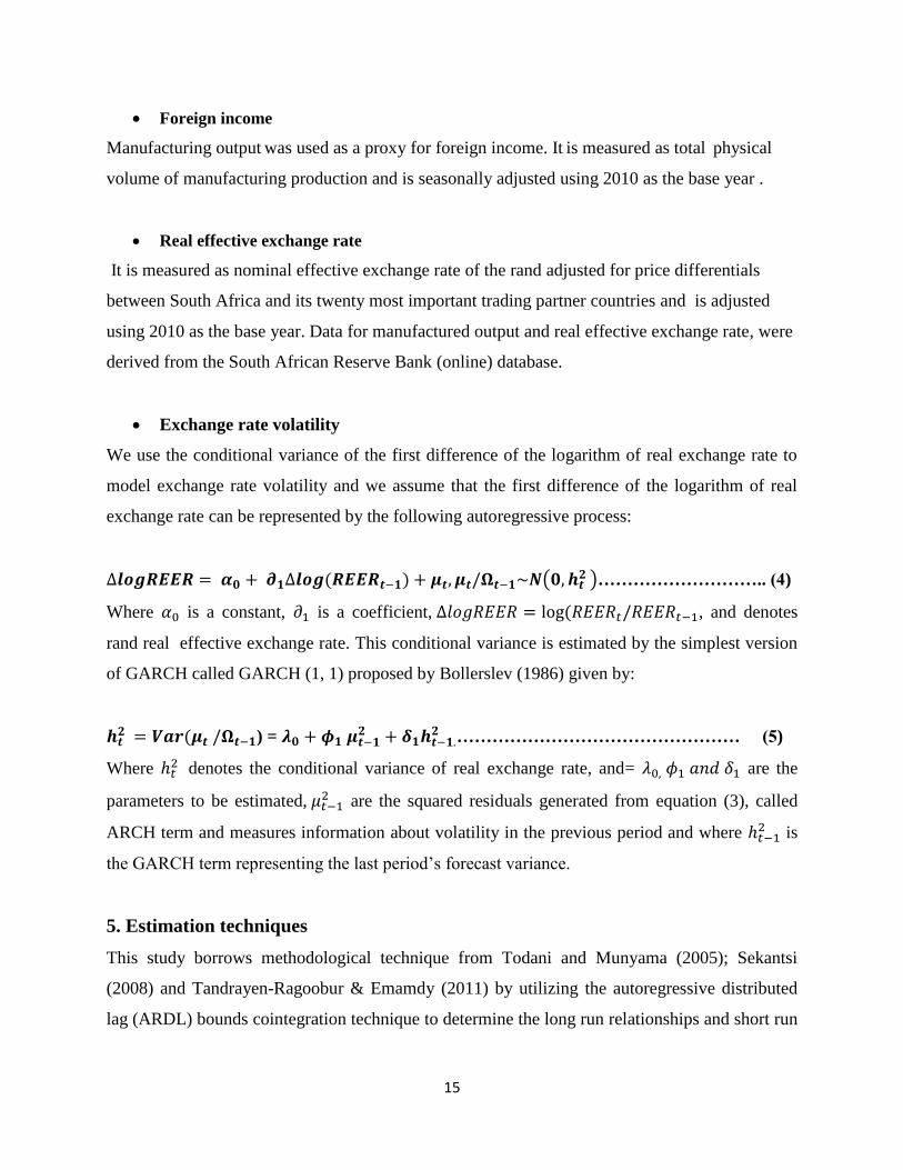
Manufacturing output was used as a proxy for foreign income. It is measured as total physical

volume of manufacturing production and is seasonally adjusted using 2010 as the base year .

Real effective exchange rate

It is measured as nominal effective exchange rate of the rand adjusted for price differentials

between South Africa and its twenty most important trading partner countries and is adjusted

using 2010 as the base year. Data for manufactured output and real effective exchange rate, were

derived from the South African Reserve Bank (online) database.

Exchange rate volatility

We use the conditional variance of the first difference of the logarithm of real exchange rate to

model exchange rate volatility and we assume that the first difference of the logarithm of real

exchange rate can be represented by the following autoregressive process:

∆𝒍𝒐𝒈𝑹𝑬𝑬𝑹 = 𝜶𝟎 + 𝝏𝟏∆𝒍𝒐𝒈(𝑹𝑬𝑬𝑹𝒕−𝟏) + 𝝁𝒕, 𝝁𝒕/𝛀𝒕−𝟏~𝑵(𝟎, 𝒉𝒕𝟐 )……………………….. (4)

Where 𝛼0 is a constant, 𝜕1 is a coefficient, ∆𝑙𝑜𝑔𝑅𝐸𝐸𝑅 = log (𝑅𝐸𝐸𝑅𝑡/𝑅𝐸𝐸𝑅𝑡−1, and denotes

rand real effective exchange rate. This conditional variance is estimated by the simplest version

of GARCH called GARCH (1, 1) proposed by Bollerslev (1986) given by:

𝒉𝒕𝟐 = 𝑽𝒂𝒓(𝝁𝒕 /𝛀𝒕−𝟏) = 𝝀𝟎 + 𝝓𝟏 𝝁𝒕−𝟏

𝟐 + 𝜹𝟏𝒉𝒕−𝟏.𝟐 ………………………………………… (5)

Where ℎ𝑡2 denotes the conditional variance of real exchange rate, and= 𝜆0, 𝜙1 𝑎𝑛𝑑 𝛿1 are the

parameters to be estimated, 𝜇𝑡−12 are the squared residuals generated from equation (3), called

ARCH term and measures information about volatility in the previous period and where ℎ𝑡−12 is

the GARCH term representing the last period’s forecast variance.

5. Estimation techniques

This study borrows methodological technique from Todani and Munyama (2005); Sekantsi

(2008) and Tandrayen-Ragoobur & Emamdy (2011) by utilizing the autoregressive distributed

lag (ARDL) bounds cointegration technique to determine the long run relationships and short run

16

dynamics between exports and regressor variables(foreign income, relative prices and real

exchange rate volatility) .

The ARDL cointegration approach was developed by Pesaran and Shin (1999) and Pesaran et al.

(2001). It has three advantages in comparison with other previous and traditional cointegration

methods. Firstly, the ARDL does not need that all the variables under study must be integrated of

the same order and it can be applied when the under-lying variables are integrated of order one,

order zero or fractionally integrated. Secondly, the ARDL test is relatively more efficient in the

case of small and finite sample data sizes. Lastly, by applying the ARDL technique, we obtain

unbiased estimates of the long-run model (Harris and Sollis, 2003).

The procedures to carry out the ARDL approach to cointegration technique include the

determination of the long run relationships among the variables by using the Bounds F-Test ; and

the estimation of the coefficients of the long and short run relationships by using the OLS

method and error correction model.

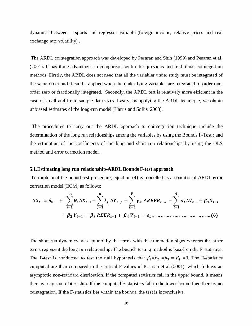
5.1.Estimating long run relationship-ARDL Bounds F-test approach

To implement the bound test procedure, equation (4) is modelled as a conditional ARDL error

correction model (ECM) as follows:

∆𝑿𝒕 = 𝜹𝟎 + ∑ 𝜽𝒊

𝒎

𝒊=𝟏

∆𝑿𝒕−𝒊 + ∑ ƛ𝒋

𝒏

𝒋=𝟏

∆𝒀𝒕−𝒋 + ∑ 𝜸𝒌

𝒑

𝒌=𝟏

∆𝑹𝑬𝑬𝑹𝒕−𝒌 + ∑ 𝜶𝒍

𝒒

𝒍=𝟏

∆𝑽𝒕−𝒍 + 𝜷𝟏𝑿𝒕−𝒍

+ 𝜷𝟐 𝒀𝒕−𝟏 + 𝜷𝟑 𝑹𝑬𝑬𝑹𝒕−𝟏 + 𝜷𝟒 𝑽𝒕−𝟏 + 𝜺𝒕 … … … … … … … … … … … … … (𝟔)

The short run dynamics are captured by the terms with the summation signs whereas the other

terms represent the long run relationship. The bounds testing method is based on the F-statistics.

The F-test is conducted to test the null hypothesis that 𝛽1=𝛽2 =𝛽3 = 𝛽4 =0. The F-statistics

computed are then compared to the critical F-values of Pesaran et al (2001), which follows an

asymptotic non-standard distribution. If the computed statistics fall in the upper bound, it means

there is long run relationship. If the computed F-statistics fall in the lower bound then there is no

cointegration. If the F-statistics lies within the bounds, the test is inconclusive.

17

5.2. Estimating short run dynamics- ARDL-ECM

After cointegration is found, the long run estimates of the ARDL model can be obtained.

Furthermore, the existence of the cointegration property means that there is the presence of an

error correction term, which shows the speed of adjustment back to the long run equilibrium as a

consequence of a short term shock. As a result, an error correction model (ECM) is estimated.

The ECM is expressed as follows:

∆𝑿𝒕 = 𝜹𝟎 + ∑ 𝜽𝒊 𝒎𝒊=𝟏 ∆𝑿𝒕−𝒊 + ∑ ƛ𝒋

𝒏𝒋=𝟏 ∆𝒀𝒕−𝒋 + ∑ 𝜸𝒌

𝒑𝒌=𝟏 ∆𝑹𝑬𝑬𝑹𝒕−𝒌 + ∑ 𝜶𝒍

𝒒𝒍=𝟏 ∆𝑽𝒕−𝒍 +

𝜷𝟏𝑿𝒕−𝟏 + 𝝅𝑬𝑪𝑴𝒕−𝟏 + 𝝁𝟏………………………………………………………………… (7)

Where:

𝜋 = the speed of adjustment parameter and

ECM = the lag residuals that are found from the estimated cointegration model.

If 𝜋 is negatively significant, then the variables tend to converge to their long run equilibrium.

5.3. Selection of lag order criteria

Selection of lag order criteria is done for each variable by using Schwarz criterion (SC). The

choice of the SC is based on the following argument:

The Bayesian information criterion or Schwarz criterion is a criterion for model selection among

a finite set of models where the model with the lowest BIC is preferred. It is based partly, on the

likelihood function and it is closely related to the AIC.

When fitting models, it is possible to increase the likelihood by adding parameters, but doing so

may result in overfitting. Though the SC and AIC resolve this problem by introducing a penalty

term for the number of parameters in the model; the penalty is larger in SC than IN AIC.

5.4. Stability tests

Finally, we examine the stability of the long-run coefficients together with the short-run

dynamics (that is, establishing the goodness of fit of the ARDL model) by applying the

18

cumulative sum of recursive residuals (CUSUM) and the cumulative sum of squares of recursive

residuals (CUSUMSQ), proposed by Brown et al. (1975). The CUSUM test uses the cumulative

sum of recursive residuals based on the first set of observations and is updated recursively and

plotted against break points. If the plot of CUSUM statistics stays within the critical bounds of 5

percent significance level (represented by a pair of straight lines drawn at the 5 percent level of

significance), the null hypothesis that all coefficients in the error correction model are stable

cannot be rejected. If either of the lines is crossed, the null hypothesis of coefficient constancy

can be rejected at the 5 percent level of significance. A similar procedure is used to carry out the

CUSUMSQ test, which is based on the squared recursive residuals.

6. Empirical Results

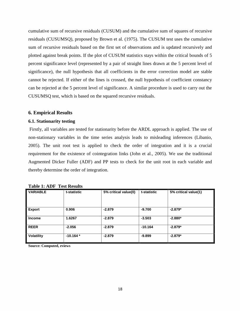
6.1. Stationarity testing

Firstly, all variables are tested for stationarity before the ARDL approach is applied. The use of

non-stationary variables in the time series analysis leads to misleading inferences (Libanio,

2005). The unit root test is applied to check the order of integration and it is a crucial

requirement for the existence of cointegration links (John et al., 2005). We use the traditional

Augmented Dicker Fuller (ADF) and PP tests to check for the unit root in each variable and

thereby determine the order of integration.

Table 1: ADF Test Results

VARIABLE t-statistic

5% critical value(0)

t-statistic

5% critical value(1)

Export 0.906 -2.879 -9.700 -2.879*

Income 1.6267 -2.879 -3.503 -2.880*

REER -2.056 -2.879 -10.164 -2.879*

Volatility -10.164 * -2.879 -9.899 -2.879*

Source: Computed, eviews

19

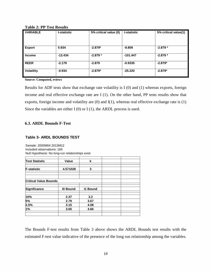
Table 2: PP Test Results

VARIABLE t-statistic

5% critical value (0) t-statistic

5% critical value(1)

Export 0.934 -2.879* -9.809 -2.879 *

Income -13.434 -2.879 * -101.447 -2.879 *

REER -2.179 -2.879 -0.9335 -2.879*

Volatility -0.934 -2.879* -25.220 -2.879*

Source: Computed, eviews

Results for ADF tests show that exchange rate volatility is I (0) and (1) whereas exports, foreign

income and real effective exchange rate are I (1). On the other hand, PP tests results show that

exports, foreign income and volatility are (0) and I(1), whereas real effective exchange rate is (1)

Since the variables are either I (0) or I (1), the ARDL process is used.

6.3. ARDL Bounds F-Test

Table 3- ARDL BOUNDS TEST

Sample: 2000M04 2013M12

Included observations: 165

Null Hypothesis: No long-run relationships exist

Test Statistic Value k

F-statistic 4.571028 3

Critical Value Bounds

Significance I0 Bound I1 Bound

10% 2.37 3.2

5% 2.79 3.67

2.5% 3.15 4.08

1% 3.65 4.66

The Bounds F-test results from Table 3 above shows the ARDL Bounds test results with the

estimated F-test value indicative of the presence of the long run relationship among the variables.

20

As the calculated F-statistic of 4.571028 exceeds the upper bound critical value (3.67), at 5%

then the null hypothesis of no cointegration is rejected.

6.4. Estimating long run relationship and short run dynamics - the ARDL approach

As cointegration is confirmed, we move to the second stage where the ARDL model can be

established to determine long run relationships and short run dynamics.

TABLE 4-ARDL Cointegrating And Long Run Form

Cointegrating Form

Variable Coefficient Std. Error t-Statistic Prob.

D(MAN__OUTPUT) 0.165505 0.061506 2.690849 0.0079

D(MAN__OUTPUT(-1)) 0.230963 0.065818 3.509127 0.0006

D(MAN__OUTPUT(-2)) 0.173775 0.062548 2.778256 0.0061

D(REER) -0.603342 0.348866 -1.729437 0.0857

D(REER(-1)) -0.070035 0.040931 -1.711063 0.0891

D(LOGREER) 34.795049 29.878562 1.164549 0.2460

CointEq(-1) -0.013788 0.002847 -4.842394 0.0000

Cointeq = PPI_EXPORT_ - (5.3577*MAN__OUTPUT + 17.6408*REER

-1497.3181*LOGREER + 4777.9458 )

Long Run Coefficients

Variable Coefficient Std. Error t-Statistic Prob.

FOREIGN INCOME 5.357651 1.824808 2.936008 0.0038

REER 17.640828 18.235200 0.967405 0.3349

LOGREER -

1497.318079 1570.668662 -0.953300 0.3419

C 4777.945805 5361.279217 0.891195 0.3742

As reported in table 4 above, the estimated coefficient of the long-run relationship is significant

for foreign income and but not significant for real effective exchange rates and exchange rate

volatility at 5 percent level. Foreign income bears a significant positive sign. This implies that

21

there is long run equilibrium between foreign income and South African exports. A positive

coefficient of 5.3577 implies that a 10 percent increase in foreign income will lead to about 54

percent increase in aggregate South African exports.

Relative prices also have a significant positive sign and a coefficient of 17.640828, but it is

statistically insignificant, implying no evidence of long-run equilibrium relationship between real

exchange rate and South African exports.

Real exchange rate volatility has a surprising positive sign and it is statistically insignificant.

This implies that there is no evidence of long-run equilibrium relationship between exchange rate

volatility and South African exports.

The coefficient of error correction term, -0.013788, is negative and statistically insignificant and is

therefore not supportive of the validity of the long-run equilibrium relationship between the

variables. The coefficient is also very small; suggesting a very slow adjustment process and indicate

what proportion of the disequilibrium is corrected each month. The coefficient implies that about 1.4

percent of the disequilibrium of the previous month’s shock adjusts back to equilibrium in the current

month.

6.6. Stability

Finally, we examine the stability of the long-run coefficients together with the short-run

dynamics by applying the CUSUM (Cumulative Sum of Recursive Residuals) and CUSUMSQ

(Cumulative Sum of Squares of Recursive Residuals) plots (Brown et al. 1975). The CUSUM

and CUSUMSQ plots for the estimated model are shown in Figure 1 and 2. If the plots of the

CUSUM and CUSUMSQ statistics stay within the critical bounds of five per cent level of

significance, the null hypothesis of all coefficients in the given regression are stable and cannot

be rejected. If CUSUM and CUSUMSQ statistics are well within the 5 percent critical bounds

that implies that short run and long run coefficients in the ARDL-Error Correction Model are

stable (Srinivasan and Kalaivani, 2013).

22

Figure 1: Plot of Cumulative Sum of Squares of Recursive Residual

-0.2

0.0

0.2

0.4

0.6

0.8

1.0

1.2

01 02 03 04 05 06 07 08 09 10 11 12 13

CUSUM of Squares 5% Significance Figure 2: Plot of Cumulative Sum of Recursive Residuals

-40

-30

-20

-10

0

10

20

30

40

01 02 03 04 05 06 07 08 09 10 11 12 13

CUSUM 5% Significance

Figures 1 and 2 show the CUSUMSQ and CUSUM plots respectively. Neither CUSUM nor

CUSUMSQ plots cross the critical bounds, indicating no evidence of any significant structural

instability.

23

7. Conclusion

This study employs the ARDL bounds test approach and monthly data for the period 2000 to

2013 to analyses the impact of exchange rate volatility on export growth in South Africa. Our

findings based on the ARDL bounds testing procedures show that volatility has a positive and

insignificant long run effect on South African exports. We also observe that foreign income has a

positive and significant long run effect on exports and this is in line with Arize e.t al, (2000).

The coefficient for foreign income bears correct positive sign (with a coefficient of 5.3577) and

is statistically significant at 5 percent level of significance, implying that a rise in foreign income

will boost South African exports.

The observed insignificant positive impact of exchange rate volatility on South African exports

implies that South Africa exporters are risk-neutral as they tend to reduce their exports

minimally. This may be attributed to availability of well-developed hedging facilities and

institutions in South Africa that can protect exporters against exchange risk.

The coefficient of the estimated Error Correction Model (ECM) is positive and insignificant.

This is an evidence of an unstable long term relationship. The coefficient of the estimated ECM

asserts that, on average, 25 percent of the departure from equilibrium value will be adjusted in

the current period. The remaining 75 percent is still to be rectified as the variables are

cointegrated. Thus, it is a fairly low speed of adjustment.

The insignificant negative impact of exchange rate on South African exports implies that

structural breaks occur during the period under review. The 2007/2008 global financial crisis can

also be cited as cause of structural instability in South Africa. The weaker rand could not boost

exports as international demand for local products was suppressed.

Labour unrests in almost all South African mines that started in the third quarter of 2012 and

ended in early 2013 can also be cited as anther cause of structural break. The weaker rand could

not boost exports as production stoppage in almost all the mines had resulted in a considerate

decline in exports.

24

We therefore recommend that, while South Africa needs to maintain competitive exchange rate

in order to sustain its exports performance, there is no need to worry about targeting at

minimizing the excessive volatility of the rand. However, the South African government should

focus on strengthening labour laws to avoid the situation that happened between 2012 and 2013, as

this may cause importers to look for alternative places where they can import

.

25

References

1. African Economic Outlook, (2008). © AfDB/OECD 2008.

2. Ahmadi-Esfahani, F. Z. (2006). Constant market shares analysis: uses, limitations and

prospects. The Australian Journal of Agricultural and Resource Economics, 50, 510-526.

3. Alexander, S.S. (1952). The Effect of a Devaluation on a Trade Balance. I.M.F. Staff

Papers, 2, 2, 263-278.

4. Arize A.C (1994) Cointegration test of a long-run relation between the real effective

exchange rate and the trade balance. International Economic Journal, volume 8, No. 3.

5. Asseery, A. & Peel, D., 1991. The effects of exchange rate volatility on exports.

Economic Letters, 37, pp. 173–177.

6. Aziakpono, M., Tsheole, T. & Takaendasa, P., 2005. Real exchange rate and its effect on

trade flows: New evidence from South Africa. [Online].Available at:

http://www.essa.org.za/download/2005Conference/Takaendesa.pdf.[Accessed on 21

April 2007].c Scholarlink Research Institute Journals, 2011 (ISSN: 2141-7024).

7. Cameron, S.; D. Kihangire and D. Potts (2005): “Has exchange rate volatility reduced

Ugandan coffee export earnings?,” Bradford Centre for International Development

(BCID), University of Bradford.

8. Clark, P.B. 1973. Uncertainty, Exchange Risk, and the Level of International Trade.

Western Economic Journal, 11: 302-313.

9. Cote A 1994. Exchange Rate Volatility and Trade: A Survey. Bank of Canada Working

Paper, 94-5.

10. De Vita, G. and A. Abbott (2004): “Real exchange rate volatility and US exports: An

ARDL bounds testing approach,” Economic Issues 9, 69-78.

11. Dell’Ariccia G 1999. Exchange Rate Fluctuations and Trade Flows: Evidence from the

European Union. IMF Staff Papers, 40: 315-334.

12. Dornbusch R 1980. Open Economy Macroeconomics. New York: Basic Books.

13. Doroodian, K., 1999. Does exchange rate volatility deter international trade in developing

countries? Journal of Asian Economics, 10 (3),pp.65-474

14. Economic Overview, 2013

26

15. Edwards, L., & Willcox, O. (2002). Exchange rate depreciation and the trade balance in

South Africa. Report Prepared for the National Treasury of Southa Africa.

16. Edwards,L.J. and Garlick, E.2008.Trade flows and the exchange rate in South Africa

School of Economics, University of Cape Town. January 2008

17. Fountas, S. and D. Bredin (1998): “Exchange rate volatility and exports: The case of

Ireland,” Applied Economics Letters, Taylor and Francis Journals 5, 301-304.

18. Franke, G (1991): “Exchange rate volatility and international trading strategy,” Journal of

19. Frankel, J. and Wei, S. (1993) “Trade Blocs and Currency Blocs,” NBER Working Paper

No. 4335.

20. Gotur P 1985. Effects of Exchange Rate Volatility on Trade: Some Further Evidence.

IMF Staff Papers. No.3: 475-512.

21. Hooper P. and Kohlhagen S. 1978. The Effect of Exchange Rate Uncertainty on the

Prices and Volume of International Trade. Journal of International Economics, 8: 483-

511.http://dx.doi.org/10.1111/j.1467-8489.2006.00364.x.International Money and

Finance 10, 1991, 292-307.

22. Johnson, H., 1969. The case of flexible exchange rates. Federal Reserve Bank of St Louis

Monthly Review, 51(6), pp. 12-24.

23. Johnson, H.G. (1967). Towards a General Theory of the Balance of Payments. In

International trade and Economic Growth: Studies in pure Theory. Cambridge, Mass:

Harvard University Press.

24. Kihangire, D., 2004. The impact of exchange rate variability on Uganda’s exports (1988-

2001). Ph.D. Thesis. University of Bradford.

25. Krugman, P., 1989. Exchange rate instability. Cambridge: The Massachusetts Institute of

Technology Press.

26. Metzler, L. (1948). The Theory of International Trade. In Howard, S.E. (1984), ed., 1, A

Survey of Contemporary Economics. Philadelphia: Blakiston. Michie, J. and Padayachee,

V. (1998). Three years after apartheid: growth employment and redistribution?

Cambridge Journal of Economics, 22, 623-635

27. Milana, C. (1988). Constant Market Shares analysis and Index number theory. European

Journal of Political Economy, 4(4), 453-478. http://dx.doi.org/10.1016/0176-

2680(88)90011-0

27

28. Miles, M.A. (1979). The Effects of Devaluation of the Trade Balance and the Balance of

Payments: Some New Results. Journal of Political economy, 87, 600-20.

MPRA Paper No. 36666, posted 15. February 2012 15:25 UTC

29. Nyahokwe, O. and N. (2013).The Impact of Exchange Rate Volatility on South African

Exports.Mediterranean Journal of Social Sciences.MCSER Publishing, Rome-Italy.Vol 4

No 3.September 2013

30. Obi et al. 2013. “Assessing the Impact of Exchange Rate Volatility on the

Competitiveness of South Africa’s Agricultural Exports.” Journal of Agricultural

Science; Vol. 5, No. 10; 2013 ISSN 1916-9752 E-ISSN 1916-9760.Published by

Canadian Center of Science and Education.227

31. Ogundipe et.al. 2013. Estimating the long run effects of exchange rate devaluation on the

trade balance of Nigeria. European Scientific Journal September 2013 edition vol.9,

No.25 ISSN: 1857 – 7881 (Print) e - ISSN 1857- 743

32. Ogunleye, E. K. (2010). “Exchange Rate Volatility and Foreign Direct Investment in

Sub-Saharan Africa: Evidences from Nigeria and South Africa”.

33. Omojimite A Comparative Analysis of the Effect of Exchange Rate Volatility on Exports

in the CFA and Non-CFA Countries of Africa.© Kamla-Raj 2010 J Soc Sci, 24(1): 23-31

(2010)

34. Omojimite, B. U. and Akpokodje, G. (2010) The Impact of Exchange Rate Reforms on

Trade Performances in Nigeria, Journal of Social Sciences, 23,1. Retrieved from

http://www.krepublishers.com.

Online at http://mpra.ub.uni-muenchen.de/36666/

35. Poonyth, D. and van Zyl, J. The impact of real exchange rate changes on south african

agricultural exports: an error correction model approach. Agrekon, Vol 39, No 4

(December 2000) Poonyth & Van Zyl 673

36. Qian, Y. and P. Varangis, “Does exchange rate volatility hinder export growth?”

Empirical Economics 19, 1994, 371-396.

Retrieved from http://www.resourcespolicy, on7/2/2010.

37. Robinson, J. (1947). The Foreign Exchanges. In Essays in the Theory of Employment.

Oxford: Blackwell.

38. Sekantsi ,L., 2007.The Impact of the real exchange rate volatility on South African

exports to the United States :A bound test approach.University of Lesotho.

28

39. Siggel, E. (2006). International competitiveness and comparative advantage: A survey

and a proposal for measurement.

Springer Science + Business Media, LLC 2006. Journal of Industry, Competition and

Trade, 6,137-159. http://dx.doi.org/10.1007/s10842-006-8430-x

40. Tandrayen-Ragoobur, V. and Emamdy, N. (2011). Does Exchange Rate Volatility Harm

Exports?Evidence from Mauritius. Journal of Emerging Trends in Economics and

Management Sciences (JETEMS) 2 (3): 146-155.The Manchester School of Economic

Social Studies, 19, 272-304. http://dx.doi.org/10.1111/j.1467-9957.1951.tb00012.x

41. Tyszynski, H. (1951). World trade in manufactured commodities, 1899-1950.

42. Umaru et al., 2005. An Empirical Analysis of Exchange Rate Volatility on Export Trade

In a Developing Economy Journal of Emerging Trends in Economics and Management

Sciences (JETEMS) 4(1): 42-53.© Scholarlink Research Institute Journals, 2013 (ISSN:

2141-7024)

43. Vergil, H., 2002. Exchange rate volatility in Turkey and its effects on trade flows.

Journal of Economic and Social Research, 4 (1), pp. 83-99.