, published 5 December 2011, doi: 10.1098/rstb.2011.0173367 2012 Phil. Trans. R. Soc. B Robertson, Sylvia Vetter, Hon Man Wong and Jo Smith
AndyJagadeesh B. Yeluripati, Emily Bottoms, Chris Brown, Jenny Farmer, Diana Feliciano, Cui Hao, Kuhnert, Dali R. Nayak, Mark Pogson, Mark Richards, Gosia Sozanska-Stanton, Shifeng Wang,Marta Dondini, Nuala Fitton, Helen Flynn, Astley Hastings, Jon Hillier, Edward O. Jones, Matthias Pete Smith, Fabrizio Albanito, Madeleine Bell, Jessica Bellarby, Sergey Blagodatskiy, Arindam Datta, researchSystems approaches in global change and biogeochemistry
Supplementary data
l http://rstb.royalsocietypublishing.org/content/suppl/2011/12/13/367.1586.311.DC1.htm
"Audio supplement"
References
http://rstb.royalsocietypublishing.org/content/367/1586/311.full.html#related-urls Article cited in:
http://rstb.royalsocietypublishing.org/content/367/1586/311.full.html#ref-list-1
This article cites 45 articles, 8 of which can be accessed free
Subject collections
(62 articles)systems biology � (207 articles)environmental science �
(448 articles)ecology � Articles on similar topics can be found in the following collections
Email alerting service hereright-hand corner of the article or click Receive free email alerts when new articles cite this article - sign up in the box at the top
http://rstb.royalsocietypublishing.org/subscriptions go to: Phil. Trans. R. Soc. BTo subscribe to
on May 16, 2013rstb.royalsocietypublishing.orgDownloaded from

on May 16, 2013rstb.royalsocietypublishing.orgDownloaded from
Phil. Trans. R. Soc. B (2012) 367, 311–321
doi:10.1098/rstb.2011.0173
Review
* Autho
One conecology:
Systems approaches in global changeand biogeochemistry research
Pete Smith*, Fabrizio Albanito, Madeleine Bell, Jessica Bellarby,
Sergey Blagodatskiy, Arindam Datta, Marta Dondini, Nuala Fitton,
Helen Flynn, Astley Hastings, Jon Hillier, Edward O. Jones,
Matthias Kuhnert, Dali R. Nayak, Mark Pogson, Mark Richards,
Gosia Sozanska-Stanton, Shifeng Wang, Jagadeesh B. Yeluripati,
Emily Bottoms, Chris Brown, Jenny Farmer, Diana Feliciano,
Cui Hao, Andy Robertson, Sylvia Vetter,
Hon Man Wong and Jo Smith
Institute of Biological and Environmental Sciences, University of Aberdeen, 23 St Machar Drive,Aberdeen AB24 3UU, UK
Systems approaches have great potential for application in predictive ecology. In this paper, we pre-sent a range of examples, where systems approaches are being developed and applied at a range ofscales in the field of global change and biogeochemical cycling. Systems approaches range fromBayesian calibration techniques at plot scale, through data assimilation methods at regional to con-tinental scales, to multi-disciplinary numerical model applications at country to global scales. Weprovide examples from a range of studies and show how these approaches are being used to addresscurrent topics in global change and biogeochemical research, such as the interaction betweencarbon and nitrogen cycles, terrestrial carbon feedbacks to climate change and the attribution ofobserved global changes to various drivers of change. We examine how transferable the methodsand techniques might be to other areas of ecosystem science and ecology.
Keywords: system biology; ecology; systems approach; global change; biogeochemistry; model
1. INTRODUCTION(a) Ecology is a systems science
Ecology, almost by definition, is a systems science.A system is defined [1] as a ‘whole compounded ofseveral parts or members’ or ‘a set of interacting orinterdependent system components forming an inte-grated whole’. Among the scientific research fieldslisted on the definition page (systems theory, cyber-netics, dynamical systems, thermodynamics andcomplex systems; [1]), ecology is not mentioned, butwhen we look at the common characteristics of systems(they have structure defined by components and theircomposition; they have behaviour, which involvesinputs, processing and outputs of material, energy,information or data; they have interconnectivityin terms of functional and structural relationshipsbetween components; and they have functions orgroups of functions), modern ecology is clearly a sys-tems science. This is further supported by thefinding that a search of Web of Knowledge on
r for correspondence ([email protected]).
tribution of 16 to a Discussion Meeting Issue ‘Predictivesystems approaches’.
311
10 March 2011, for articles containing the keywords‘ecology’ and ‘system’ for the 10 years 2001–2010,yielded more than 100 000 results.
Ecologists, and other scientists involved in model-ling ecological or ecosystem interactions, have longconsidered themselves to be systems scientists.Indeed, since the 1990s, a number of biogeochemicalor ecological modelling papers have been publishedin systems analysis journals [2]. If, in the late 1990s,we ecological modellers had been asked whether weconsidered ourselves to be working in ‘systemsbiology’, the majority of us would probably haveanswered ‘yes’. If we were to be asked the same ques-tion now, perhaps far fewer of us would answer in theaffirmative, since systems biology has largely come tomean something different. Systems biology is nowoften (but not exclusively) associated with rathersmall-scale processes (from the gene to the organism),with the majority of projects under recent UK systemsbiology initiatives operating at these scales [3]. Someof the authors of this paper attended a systems biologytalk at the University of Aberdeen in 2008 entitled‘Modelling across scales’—the scales in questionturned out to be from the gene to the cell! For theecological and ecosystem modellers, the talk, while
This journal is q 2011 The Royal Society
emissions and land demand: climate input drivers:
biological input drivers:NPP – Lund PotsdamJena (LPJ) model [12]soil geographical data(pedotransfer functions;JRC; [13])
climate models(HadCM3, PCM,CSIRO2, CGCM2; [4])
land-use change:
biospheric processes (IMAGE 2.0; [7])
emission scenario models [8]
regional climatedownscaling models [4]
soil C model:RothC [9]
energy sector and greenhouse gas emissions [7]
socioeconomic drivers [7,8]
— —
—
—
—
—
—
human and physicalgeography and technologydevelopment [10, 11]economic decision-making(autonomous adaptation; [11])resource base (IMAGE 2.0and UCL land-use changemodel; [11])
— —
—
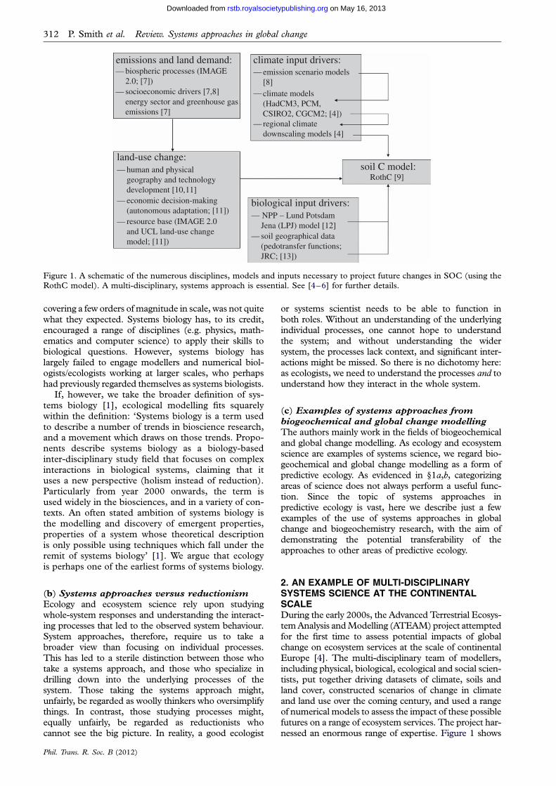
Figure 1. A schematic of the numerous disciplines, models and inputs necessary to project future changes in SOC (using theRothC model). A multi-disciplinary, systems approach is essential. See [4–6] for further details.
312 P. Smith et al. Review. Systems approaches in global change
on May 16, 2013rstb.royalsocietypublishing.orgDownloaded from
covering a few orders of magnitude in scale, was not quitewhat they expected. Systems biology has, to its credit,encouraged a range of disciplines (e.g. physics, math-ematics and computer science) to apply their skills tobiological questions. However, systems biology haslargely failed to engage modellers and numerical biol-ogists/ecologists working at larger scales, who perhapshad previously regarded themselves as systems biologists.
If, however, we take the broader definition of sys-tems biology [1], ecological modelling fits squarelywithin the definition: ‘Systems biology is a term usedto describe a number of trends in bioscience research,and a movement which draws on those trends. Propo-nents describe systems biology as a biology-basedinter-disciplinary study field that focuses on complexinteractions in biological systems, claiming that ituses a new perspective (holism instead of reduction).Particularly from year 2000 onwards, the term isused widely in the biosciences, and in a variety of con-texts. An often stated ambition of systems biology isthe modelling and discovery of emergent properties,properties of a system whose theoretical descriptionis only possible using techniques which fall under theremit of systems biology’ [1]. We argue that ecologyis perhaps one of the earliest forms of systems biology.
(b) Systems approaches versus reductionism
Ecology and ecosystem science rely upon studyingwhole-system responses and understanding the interact-ing processes that led to the observed system behaviour.System approaches, therefore, require us to take abroader view than focusing on individual processes.This has led to a sterile distinction between those whotake a systems approach, and those who specialize indrilling down into the underlying processes of thesystem. Those taking the systems approach might,unfairly, be regarded as woolly thinkers who oversimplifythings. In contrast, those studying processes might,equally unfairly, be regarded as reductionists whocannot see the big picture. In reality, a good ecologist
Phil. Trans. R. Soc. B (2012)
or systems scientist needs to be able to function inboth roles. Without an understanding of the underlyingindividual processes, one cannot hope to understandthe system; and without understanding the widersystem, the processes lack context, and significant inter-actions might be missed. So there is no dichotomy here:as ecologists, we need to understand the processes and tounderstand how they interact in the whole system.
(c) Examples of systems approaches from
biogeochemical and global change modelling
The authors mainly work in the fields of biogeochemicaland global change modelling. As ecology and ecosystemscience are examples of systems science, we regard bio-geochemical and global change modelling as a form ofpredictive ecology. As evidenced in §1a,b, categorizingareas of science does not always perform a useful func-tion. Since the topic of systems approaches inpredictive ecology is vast, here we describe just a fewexamples of the use of systems approaches in globalchange and biogeochemistry research, with the aim ofdemonstrating the potential transferability of theapproaches to other areas of predictive ecology.
2. AN EXAMPLE OF MULTI-DISCIPLINARYSYSTEMS SCIENCE AT THE CONTINENTALSCALEDuring the early 2000s, the Advanced Terrestrial Ecosys-tem Analysis and Modelling (ATEAM) project attemptedfor the first time to assess potential impacts of globalchange on ecosystem services at the scale of continentalEurope [4]. The multi-disciplinary team of modellers,including physical, biological, ecological and social scien-tists, put together driving datasets of climate, soils andland cover, constructed scenarios of change in climateand land use over the coming century, and used a rangeof numerical models to assess the impact of these possiblefutures on a range of ecosystem services. The project har-nessed an enormous range of expertise. Figure 1 shows
–10°(a) (b)10° 20° 30°
60°
50°
40°
60°
50°
40°
0°
0
tC ha–1
> 20 15 10 5 2 0 –2 –5 –10 –15
500 1000 1500 km 0 500 1000 1500 km
–10° 10° 20° 30°0°
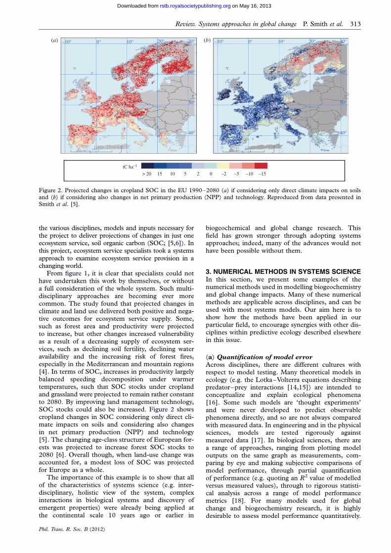
Figure 2. Projected changes in cropland SOC in the EU 1990–2080 (a) if considering only direct climate impacts on soilsand (b) if considering also changes in net primary production (NPP) and technology. Reproduced from data presented inSmith et al. [5].
Review. Systems approaches in global change P. Smith et al. 313
on May 16, 2013rstb.royalsocietypublishing.orgDownloaded from
the various disciplines, models and inputs necessary forthe project to deliver projections of changes in just oneecosystem service, soil organic carbon (SOC; [5,6]). Inthis project, ecosystem service specialists took a systemsapproach to examine ecosystem service provision in achanging world.
From figure 1, it is clear that specialists could nothave undertaken this work by themselves, or withouta full consideration of the whole system. Such multi-disciplinary approaches are becoming ever morecommon. The study found that projected changes inclimate and land use delivered both positive and nega-tive outcomes for ecosystem service supply. Some,such as forest area and productivity were projectedto increase, but other changes increased vulnerabilityas a result of a decreasing supply of ecosystem ser-vices, such as declining soil fertility, declining wateravailability and the increasing risk of forest fires,especially in the Mediterranean and mountain regions[4]. In terms of SOC, increases in productivity largelybalanced speeding decomposition under warmertemperatures, such that SOC stocks under croplandand grassland were projected to remain rather constantto 2080. By improving land management technology,SOC stocks could also be increased. Figure 2 showscropland changes in SOC considering only direct cli-mate impacts on soils and considering also changesin net primary production (NPP) and technology[5]. The changing age-class structure of European for-ests was projected to increase forest SOC stocks to2080 [6]. Overall though, when land-use change wasaccounted for, a modest loss of SOC was projectedfor Europe as a whole.
The importance of this example is to show that allof the characteristics of systems science (e.g. inter-disciplinary, holistic view of the system, complexinteractions in biological systems and discovery ofemergent properties) were already being applied atthe continental scale 10 years ago or earlier in
Phil. Trans. R. Soc. B (2012)
biogeochemical and global change research. Thisfield has grown stronger through adopting systemsapproaches; indeed, many of the advances would nothave been possible without them.
3. NUMERICAL METHODS IN SYSTEMS SCIENCEIn this section, we present some examples of thenumerical methods used in modelling biogeochemistryand global change impacts. Many of these numericalmethods are applicable across disciplines, and can beused with most systems models. Our aim here is toshow how the methods have been applied in ourparticular field, to encourage synergies with other dis-ciplines within predictive ecology described elsewherein this issue.
(a) Quantification of model error
Across disciplines, there are different cultures withrespect to model testing. Many theoretical models inecology (e.g. the Lotka–Volterra equations describingpredator–prey interactions [14,15]) are intended toconceptualize and explain ecological phenomena[16]. Some such models are ‘thought experiments’and were never developed to predict observablephenomena directly, and so are not always comparedwith measured data. In engineering and in the physicalsciences, models are tested rigorously againstmeasured data [17]. In biological sciences, there area range of approaches, ranging from plotting modeloutputs on the same graph as measurements, com-paring by eye and making subjective comparisons ofmodel performance, through partial quantificationof performance (e.g. quoting an R2 value of modelledversus measured values), through to rigorous statisti-cal analysis across a range of model performancemetrics [18]. For many models used for globalchange and biogeochemistry research, it is highlydesirable to assess model performance quantitatively.

314 P. Smith et al. Review. Systems approaches in global change
on May 16, 2013rstb.royalsocietypublishing.orgDownloaded from
Smith et al. [18] collated a range of statistical metricsto compare model outputs with measured data andthese are available within a spreadsheet as ModEvalv. 2.0 [16]. Depending on the quality of the measureddata available, the statistics provided allow the modelerror to be quantified, as well as bias (consistentunder- or over-prediction), association, coincidenceand the separation of error owing to the model fromthat inherent within the measurements.
The statistics presented in ModEval v. 2.0 havebeen used many times in model comparisons ([18]had been cited 337 times on 10 March 2011; [19]),most recently in a comparison of the performance ofagro-ecosystem models in simulating components ofthe European cropland carbon budget [20]. Quantitat-ive methods for model comparison are now widelyavailable, and can be used in all aspects of modeldevelopment for predictive ecology.
(b) Sensitivity and uncertainty analysis
When building a numerical model, one needs to testhow the model outputs vary with changes in themodel inputs or internal model parameters. This isdone through sensitivity analysis and uncertaintyanalysis. Sensitivity analysis identifies which modelcomponents exert the most influence on the modelresults. It compares changes in simulated valuesagainst changes in the model components: these com-ponents could be input variables or internal modelparameters. Sensitivity analysis determines howhighly correlated the model result is to the value of agiven input component: does a small change in theinput cause a significant change in the output? If thisis the case, the model is termed sensitive to the input.Uncertainty analysis determines how the variabilityin the input is propagated through the model andquantifies how this is translated into variability (uncer-tainty) in the model output. If this is the case, theinput is termed important. A sensitivity analysis andan uncertainty analysis do not necessarily identify thesame inputs. A model is always sensitive to the import-ant inputs that contribute most to model outputuncertainty, since the variability will not appear inthe model output unless the model is also sensitiveto the input. However, an input to which the modelis sensitive is not necessarily important: it does notnecessarily contribute to output uncertainty since itsvalue may be known precisely [16].
(i) Sensitivity analysisWith simple models, the sensitivity of a model can betested either by changing, one at a time, an input vari-able (or internal model parameter) within a range andexamining the effect on model outputs, or all variables/parameters can be varied within the range simul-taneously (the latter is termed global sensitivityanalysis). The ratio of the change in input variable(or internal parameter) to the change in the outputvariable indicates the model sensitivity to that inputvariable (or internal parameter; [16]).
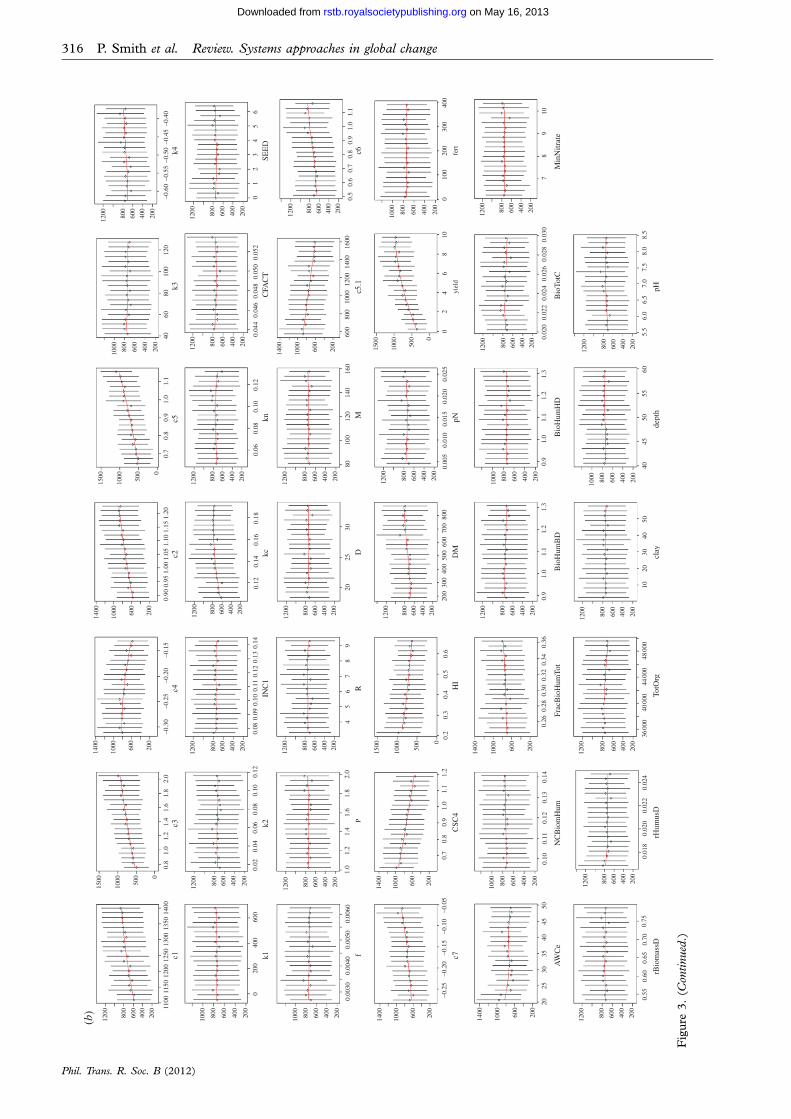
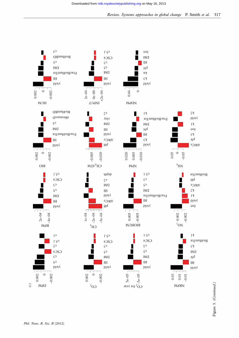
For more complex models, however, the processcan be trickier. Figure 3 shows a sensitivity analysisof the ECOSSE model [21,22], which is used for
Phil. Trans. R. Soc. B (2012)
simulating soil carbon and nitrogen turnover andgreenhouse gas emissions from soils. Two thousandMonte Carlo simulations were run using a weathergenerator [23], varying 40 soil and crop parameterswithin realistic ranges. Twenty response variableswere examined. Owing to the complexity of themodel, the relationships between inputs and outputsare somewhat unclear (figure 3a shows the depend-ence of the decomposable plant material (DPM)SOC fraction on variations in a range of internalmodel parameters and input variables). To elucidatethe relationships from the output, the data werebinned (i.e. grouped within fixed ranges of the par-ameter values) and a smooth spline was fittedthrough the means of the bins, making the relationshipclearer. The degrees of freedom in the spline werechosen to reduce scatter, but also to allow nonlinearity(figure 3b). From this, the most important sensitivitiesin the model can be determined, where the sensitivityindex is the variance in the smooth spline through thebins/total variance (note: sum of sensitivities nolonger ¼ 100%; figure 3c). This method demonstratesthat sensitivity analysis is possible even for complexmodels, and that metrics are available for comparingrelative sensitivity. The method is applicable to arange of numerical models.
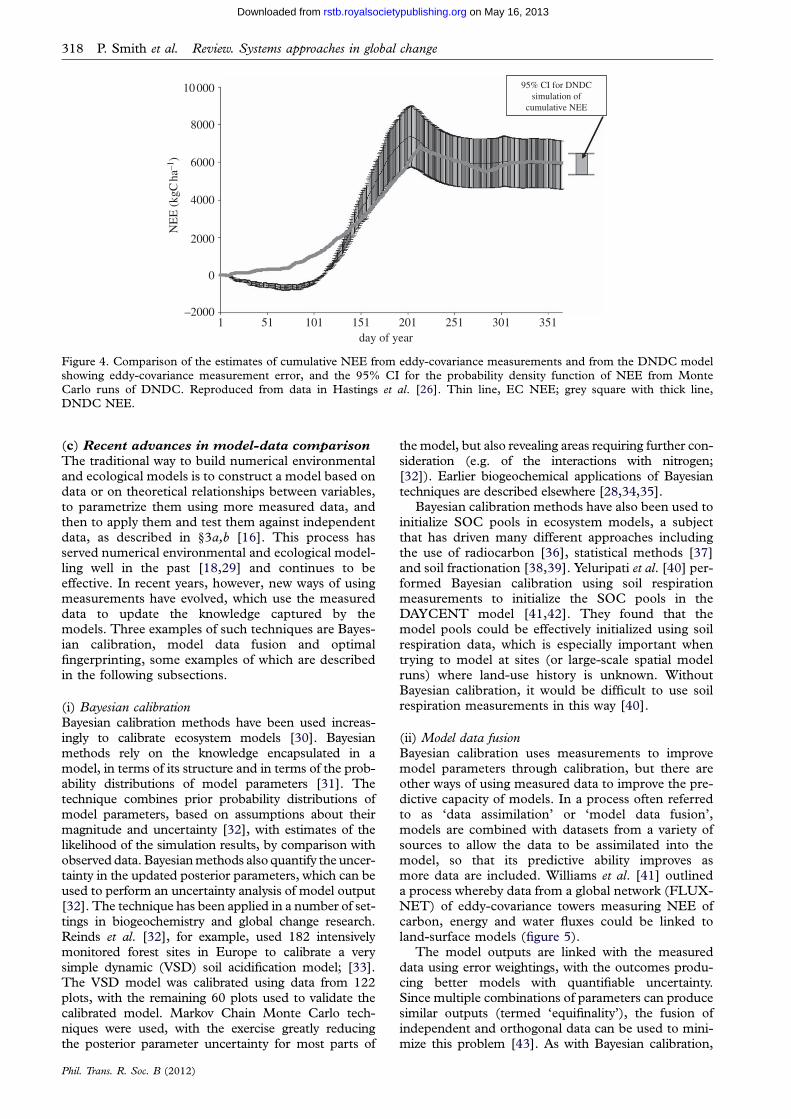
(ii) Uncertainty analysisThere have been a number of recent advances in asses-sing uncertainty in model outputs. One of thesetechniques, Bayesian calibration, is discussed further in§3c, so will not be further discussed here. Gottschalket al. [24] used Monte Carlo techniques to examine therole of measurement uncertainties in assessing estimatesof net ecosystem exchange (NEE) in European grass-lands, using the PaSim model [25]. Global uncertainty[16] was compared across 2 years and across sites. Theanalysis revealed considerable variation in global uncer-tainty from site to site and between years, indicatingthat output uncertainty does not depend solely on absol-ute input uncertainties, and suggesting that case specificuncertainty analysis is required. Hastings et al. [26]quantified uncertainty propagation through the DeNitri-fication DeComposition (DNDC) model on a croplandsite, finding that the overall impact of uncertainty ininput parameters on predicted biogenic greenhouse gasemissions was relatively small. Indeed, the studysuggested that the 95% CI of the DNDC predictionsof NEE were smaller than the error associated with theeddy-covariance measurements (figure 4).
Other developments in uncertainty analysis includemethods to combine uncertainties, including, forexample, expert judgement of error (measurement),analytical uncertainty (measurement), sampling uncer-tainty (measurement), conceptual uncertainty (model)and scenario uncertainty (model; [27]). Other categoriz-ations of the components of uncertainty have beenproposed, and schemes to combine these differentuncertainty components have been developed [28]. Ascomputing capacity has increased in recent years, andtechniques for comparing components, and partitioningthe sources, of uncertainty in numerical models haveimproved, so has the quantification of uncertainty inmodel outputs.

2500
(a)
1500 500 0
2500
1500 500 0
2500
1500 500 0
2500
1500 500 0
2500
1500 500 0
2500
1500 500 0
0
0.00
3
0.5 0 6
78
Min
Nitr
ate9
100.
550.
600.
65
rBio
mas
sDrH
umus
DTo
tOrg
clay
dept
hpH
0.70
0.75
0.80
0.01
80.
020
0.02
20.
024
35 0
0040
000
45 0
0050
000
010
2030
4050
6040
4550
5560
5.5
6.0
6.5
7.0
7.5
8.0
8.5
100
200
fert
AW
Ce
NC
Bio
mH
um30
040
020
2530
3540
4550
0.10
0.11
0.12
0.13
0.14
0.24
0.26
0.28
0.30
Frac
Bio
Hum
Tot
Bio
Hum
BD
Bio
Hum
HD
Bio
TotC
0.32
0.34
0.36
0.9
1.0
1.1
1.2
1.3
0.9
1.0
1.1
1.2
1.3
0.02
00.
022
0.02
40.
026
0.02
80.
030
0.6
0.7
0.8
0.9
1.0
1.1
1.2
–0.2
5–0
.20
–0.1
5–0
.10
–0.0
50.
60.
70.
80.
91.
01.
11.
20.
20.
30.
40.
50.
620
040
060
080
00.
005
0.01
00.
015
0.02
00.
025
02
46
810
0.00
4
f c6c7
CSC
4H
ID
IMpN
yiel
d
0.00
50.
006
1.0
1.2
1.4
P
1.6
1.8
2.0
4.0
4.5
5.0 L
5.5
6.0
34
56
R
78
920
25
D
3080
100
120
M
140
160
600
800
1000 c5
. 1
1200
1400
1600
200
400
k1k2
INC
1kc
knC
FAC
TSE
ED
600
0.02
0.04
0.06
0.08
0.08
0.10
0.10
0.12
0.12
0.12
0.14
0.16
0.18
0.06
0.08
0.10
0.12
0.04
40.
046
0.04
80.
050
0.05
20.
054
01
23
45
60.
14
1100
1150
1200
1250 c1
1300
1350
1400
0.8
1.0
1.2
1.4
c3c4
c2c5
k3k4
1.6
1.8
2.0
–0.3
0–0
.25
–0.2
0–0
.15
0.90
1.00
1.10
1.20
0.7
0.8
0.9
1.0
1.1
4060
8010
012
0–0
.60
–0.5
5–0
.50
–0.4
5–0
.40
Fig
ure
3.(C
ontinued
.)S
plin
efi
ttin
gfo
rse
nsi
tivit
yan
aly
sis
ofco
mple
xm
od
els.
(a)
Plo
tsofva
riati
on
sin
mod
elpools
(in
this
case
raw
ou
tpu
tson
the
dec
om
posa
ble
pla
nt
mat
eria
l(D
PM
)pool
of
the
EC
OS
SE
mod
el[2
1,2
2])
acco
rdin
gto
vari
ati
on
sin
mod
elin
tern
alpara
met
ers
an
din
pu
tva
riable
s,(b
)plo
tsof
splin
esfi
tted
thro
ugh
the
mea
ns
of
dat
aaft
erpoolin
gin
bin
s,re
vealin
gth
etr
end
sin
the
resp
on
ses,
(c)
the
sen
siti
vit
yof
all
soil
carb
on
an
dn
itro
gen
pools
inE
CO
SS
Eto
vari
ati
on
sin
inte
rnal
para
met
ers
an
din
pu
tvari
able
s,af
ter
sim
ilar
an
aly
sis
des
crib
edfo
r
DP
Min
(a,b
).D
etails
of
the
para
met
ers/
vari
able
sare
un
import
an
tin
dem
on
stra
tin
gth
em
ethod
.
Review. Systems approaches in global change P. Smith et al. 315
Phil. Trans. R. Soc. B (2012)
on May 16, 2013rstb.royalsocietypublishing.orgDownloaded from
1200
(b)
1500
1400
1000 600
200
1400
1000 600
200
–0.3
0–0
.25
–0.2
0–0
.15
0.90
0.95
1.00
1.05
1.10
1.15
1.20
0.7
0.8
0.9
1.0
1.1
4060
8010
012
0–0
.60
–0.5
5–0
.50
–0.4
5–0
.40
1000 500 0
1500
1000 50
0
1000 80
0
600
400
200
0
800
600
400
200
1200 80
0
600
400
200
1100
1150
1200
1250 c1 k1 f c7
AW
Ce
rBio
mas
sDrH
umus
DTo
tOr g
clay
dept
hpH
NC
Bio
mH
umFr
acB
ioH
umTo
tB
ioH
umB
DB
ioH
umH
DB
ioTo
tCM
inN
itrat
e
CSC
4H
ID
MpN
RD
Mc5
.1c6
k2IN
C1
kckn
CFA
CT
SEE
D
c3c4
c2c5
k3k4
1300
1350
1400
0.8
1.0
1.2
1.4
1.6
1.8
2.0
1200 800
1000 800
600
400
200
0
0.00
30
–0.2
5–0
.20
–0.1
5–0
.10
–0.0
50.
70.
80.
91.
01.
11.
20.
20.
30.
40.
50.
620
030
040
050
060
070
080
00.
005
0.01
00.
015
0.02
00.
025
0.00
400.
0050
0.00
601.
01.
21.
4
P
1.6
1.8
2.0
45
67
89
2025
3080
100
120
140
160
600
800
1000
1200
1400
1600
200
400
600
0.02
0.04
0.06
0.08
0.10
0.12
0.08
0.09
0.10
0.11
0.13
0.12
0.12
0.14
0.16
0.18
0.06
0.08
0.10
0.12
0.04
40.
046
0.04
80.
050
0.05
20
12
34
56
0.5
0.6
0.7
0.8
0.9
1.0
1.1
0.14
1000 800
600
400
200
600
400
200
1200 800
600
400
200
1200 800
600
400
200
1200 800
600
400
200
1200 800
600
400
200
1200
1000 80
0
600
400
200
1000 80
0
600
400
200
800
600
400
200
1200 800
600
400
200
1200 800
600
400
200
1200 800
600
400
200
1200 800
600
400
200
1200
1500
1000 80
0
600
400
200
500
1000 0
02
46
yiel
dfe
rt
810
010
020
030
040
0
800
600
400
200
1200 80
0
600
400
200
1200 80
0
600
400
200
1200 80
0
600
400
200
1200
1400
1000 60
0
200
1400
1000 600
200
1400
1000 600
200
20
0.55
0.60
0.65
0.70
0.75
0.01
80.
020
0.02
20.
024
36 0
0040
000
44 0
0048
000
1020
3040
5040
4550
5560
5.5
6.0
6.5
7.0
7.5
8.0
8.5
2530
3540
4550
0.10
0.11
0.12
0.13
0.14
0.26
0.28
0.30
0.32
0.34
0.36
0.9
1.0
1.1
1.2
1.3
0.9
1.0
1.1
1.2
1.3
0.02
00.
022
0.02
40.
026
0.02
80.
030
78
910
1400
1000 600
200
1000 800
400
600
200
1400
1000 600
200
1500
1000 500 0
800
600
400
200
1200 80
0
600
400
200
1200 800
600
400
200
1200 800
600
400
200
1200 80
0
600
400
200
1200 80
0
600
400
200
1200 80
0
600
400
200
Fig
ure
3.
(Con
tinued
.)
316 P. Smith et al. Review. Systems approaches in global change
Phil. Trans. R. Soc. B (2012)
on May 16, 2013rstb.royalsocietypublishing.orgDownloaded from
0.00
2
(c)
2e–0
40.
002
0.00
2
–0.0
02
2e–0
4
+2e
–04
0.04 0
0e–0
00
–0.0
02
–0.0
05
–0.0
20
0.02
0
0.05
–0.0
50
0.00
5
–0.0
100
–4e–
04
–5e–
04
0.00
5
0.00
2
–0.0
02
–0.0
05
–2e–
04
1e–0
4
–0.0
020
yieldc5
c3
c2
c1
c5.1
CSC4
yieldHI
DM
c3
c5.1
CSC4
c5
yield
yield
yield
yield
HI
HI
HI
HI
pN
pN
DM
DM
DM
DM
FracBioHumTot
BioHumTot
FracBioHumTot
c3
c3
k3
kn
k3
k1
k1
k2
AWCe
AWCe
pH
pN
k3
k2
fert
k1
fert
c5.1
c5.1
CSC4
c5
yield
yield
yield
HI
pN
k3
k1
fert
BioHumTot
DM
c5
pHAWCe
yield
DM
depth
c2
HI
pHAWCe
yield
yield
DM
DM
c2
c5c3
CSC4
c5.1
clay
HI
HI
yield
HI
DM
c3
c5.1
CSC4
c5
yield
HI
FracBioHumTot
c5
BioHumBD
rBiomassD
DM
yield
HI
FracBioHumTot
c5
c3
BioHumBD
DM
0.00
2
–0.0
02
–5e–
05
0.03
0.01
NRPMCO2 for yearCO2DPM
RPM
BIO
HUM INPUT NDPM
CH4ATM NPM NH4
CH4 BIOHUM NO3
–0.0
1
5e–0
50
Fig
ure
3.
(Con
tinued
.)
Review. Systems approaches in global change P. Smith et al. 317
Phil. Trans. R. Soc. B (2012)
on May 16, 2013rstb.royalsocietypublishing.orgDownloaded from
10 000
8000
6000
4000
2000
NE
E (
kgC
ha–1
)
–2000
0
1 51 101 151 201day of year
251 301
95% CI for DNDC simulation of
cumulative NEE
351
Figure 4. Comparison of the estimates of cumulative NEE from eddy-covariance measurements and from the DNDC modelshowing eddy-covariance measurement error, and the 95% CI for the probability density function of NEE from MonteCarlo runs of DNDC. Reproduced from data in Hastings et al. [26]. Thin line, EC NEE; grey square with thick line,
DNDC NEE.
318 P. Smith et al. Review. Systems approaches in global change
on May 16, 2013rstb.royalsocietypublishing.orgDownloaded from
(c) Recent advances in model-data comparison
The traditional way to build numerical environmentaland ecological models is to construct a model based ondata or on theoretical relationships between variables,to parametrize them using more measured data, andthen to apply them and test them against independentdata, as described in §3a,b [16]. This process hasserved numerical environmental and ecological model-ling well in the past [18,29] and continues to beeffective. In recent years, however, new ways of usingmeasurements have evolved, which use the measureddata to update the knowledge captured by themodels. Three examples of such techniques are Bayes-ian calibration, model data fusion and optimalfingerprinting, some examples of which are describedin the following subsections.
(i) Bayesian calibrationBayesian calibration methods have been used increas-ingly to calibrate ecosystem models [30]. Bayesianmethods rely on the knowledge encapsulated in amodel, in terms of its structure and in terms of the prob-ability distributions of model parameters [31]. Thetechnique combines prior probability distributions ofmodel parameters, based on assumptions about theirmagnitude and uncertainty [32], with estimates of thelikelihood of the simulation results, by comparison withobserved data. Bayesian methods also quantify the uncer-tainty in the updated posterior parameters, which can beused to perform an uncertainty analysis of model output[32]. The technique has been applied in a number of set-tings in biogeochemistry and global change research.Reinds et al. [32], for example, used 182 intensivelymonitored forest sites in Europe to calibrate a verysimple dynamic (VSD) soil acidification model; [33].The VSD model was calibrated using data from 122plots, with the remaining 60 plots used to validate thecalibrated model. Markov Chain Monte Carlo tech-niques were used, with the exercise greatly reducingthe posterior parameter uncertainty for most parts of
Phil. Trans. R. Soc. B (2012)
the model, but also revealing areas requiring further con-sideration (e.g. of the interactions with nitrogen;[32]). Earlier biogeochemical applications of Bayesiantechniques are described elsewhere [28,34,35].
Bayesian calibration methods have also been used toinitialize SOC pools in ecosystem models, a subjectthat has driven many different approaches includingthe use of radiocarbon [36], statistical methods [37]and soil fractionation [38,39]. Yeluripati et al. [40] per-formed Bayesian calibration using soil respirationmeasurements to initialize the SOC pools in theDAYCENT model [41,42]. They found that themodel pools could be effectively initialized using soilrespiration data, which is especially important whentrying to model at sites (or large-scale spatial modelruns) where land-use history is unknown. WithoutBayesian calibration, it would be difficult to use soilrespiration measurements in this way [40].
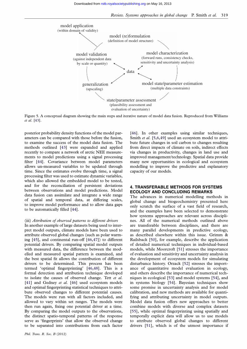
(ii) Model data fusionBayesian calibration uses measurements to improvemodel parameters through calibration, but there areother ways of using measured data to improve the pre-dictive capacity of models. In a process often referredto as ‘data assimilation’ or ‘model data fusion’,models are combined with datasets from a variety ofsources to allow the data to be assimilated into themodel, so that its predictive ability improves asmore data are included. Williams et al. [41] outlineda process whereby data from a global network (FLUX-NET) of eddy-covariance towers measuring NEE ofcarbon, energy and water fluxes could be linked toland-surface models (figure 5).
The model outputs are linked with the measureddata using error weightings, with the outcomes produ-cing better models with quantifiable uncertainty.Since multiple combinations of parameters can producesimilar outputs (termed ‘equifinality’), the fusion ofindependent and orthogonal data can be used to mini-mize this problem [43]. As with Bayesian calibration,
model application(within domain of validity)
model (re)formulation(definition of model structure)
state/parameter assessment(plausibility assessment andevaluation of uncertainty)
data
model characterization(forward runs, consistency checks,
sensitivity and uncertainty analysis)
model validation(against independent data
by scale or quantity)
generalization(upscaling)
model state/parameter estimation(multiple data constraints)
Figure 5. A conceptual diagram showing the main steps and iterative nature of model data fusion. Reproduced from Williams
et al. [43].
Review. Systems approaches in global change P. Smith et al. 319
on May 16, 2013rstb.royalsocietypublishing.orgDownloaded from
posterior probability density functions of the model par-ameters can be compared with those before the fusion,to examine the success of the model data fusion. Themethods outlined [43] were expanded and appliedrecently to compare a network of arctic NEE measure-ments to model predictions using a signal processingfilter [44]. Covariance between model parametersallows un-measured variables to be updated throughtime. Since the estimates evolve through time, a signalprocessing filter was used to estimate dynamic variables,which also allowed the embedded model to be tested,and for the reconciliation of persistent deviationsbetween observations and model predictions. Modeldata fusion can assimilate and integrate a wide rangeof spatial and temporal data, at differing scales,to improve model performance and to allow data gapsto be automatically filled [44].
(iii) Attribution of observed patterns to different driversIn another example of large datasets being used to inter-pret model outputs, climate models have been used toattribute observed global changes (such as polar warm-ing [45], and continental run-off [46,47]) to differentpotential drivers. By comparing spatial model outputswith measured data, the difference between the mod-elled and measured spatial pattern is examined, andthe best spatial fit allows the contribution of differentdrivers to be determined. This process has beentermed ‘optimal fingerprinting’ [46,48]. This is aformal detection and attribution technique developedto isolate the causes of observed change. Tett et al.[41] and Gedney et al. [46] used ecosystem modelsand optimal fingerprinting statistical techniques to attri-bute observed changes to different potential causes.The models were run with all factors included, andallowed to vary within set ranges. The models werethen run again, fixing one potential driver at a time.By comparing the model outputs to the observations,the distinct spatio-temporal patterns of the responseserve as ‘fingerprints’ that allow the observed changeto be separated into contributions from each factor
Phil. Trans. R. Soc. B (2012)
[46]. In other examples using similar techniques,Smith et al. [5,6,49] used an ecosystem model to attri-bute future changes in soil carbon to changes resultingfrom direct impacts of climate on soils, indirect effectsvia changes in productivity, changes in land use andimproved management/technology. Spatial data providemany new opportunities in ecological and ecosystemmodelling to improve the predictive and explanatorycapacity of our models.
4. TRANSFERABLE METHODS FOR SYSTEMSECOLOGY AND CONCLUDING REMARKSThe advances in numerical modelling methods inglobal change and biogeochemistry presented hereonly scratch the surface of a vast field of research,and the examples have been selected to demonstratehow systems approaches are relevant across discipli-nes. All of the numerical methods outlined aboveare transferable between disciplines, and there aremany parallel developments in predictive ecology,as described elsewhere within this issue. Grimm &Railsback [50], for example, describe the applicationof detailed numerical techniques in individual-basedmodels, while Moorcroft [51] stresses the importanceof evaluation and sensitivity and uncertainty analysis inthe development of ecosystem models for simulatingdisturbance history. Orzack [52] stresses the import-ance of quantitative model evaluation in ecology,and others describe the importance of numerical tech-niques in ecological [53] and model systems [54], andin systems biology [54]. Bayesian techniques showsome promise in uncertainty analysis and for modelcalibration, and new methods are available for quanti-fying and attributing uncertainty in model outputs.Model data fusion offers new approaches to bettercombine models with diverse and complex datasets[55], while optimal fingerprinting using spatially andtemporally explicit data will allow us to use modelsto attribute observed global changes to differentdrivers [51], which is of the utmost importance if
320 P. Smith et al. Review. Systems approaches in global change
on May 16, 2013rstb.royalsocietypublishing.orgDownloaded from
we are to manage our planet to mitigate adverseimpacts and to maximize benefits. As we increasinglyemploy systems approaches, and conduct research inmulti-disciplinary teams, the transfer of skills, tech-niques and ideas across disciplines offers excitingopportunities for predictive ecology.
This work was prepared for a conference, ‘Predictiveecology: systems approaches’ held at the Royal Society inLondon on 18–19 April 2011. P.S. is a Royal Society–Wolfson Research Merit Award holder.
REFERENCES1 Wikipedia 2011 See http://en.wikipedia.org/wiki/Main_
Page (accessed 12 March 2011).2 Smith, J. U., Bradbury, N. J., Glendining, M. J. & Smith,
P. 1997 Application of SUNDIAL to simulate nitrogenturnover in crop rotations. Quant. Approaches Syst.Anal. 10, 87–92.
3 BBSRC 2011 Search terms: ‘system’ and ‘biology’, 1622records. See http://www.bbsrc.ac.uk/pa/grants/SearchResults.aspx (accessed 12 March 2011).
4 Schroter, D. et al. 2005 Ecosystem service supply andhuman vulnerability to global change in Europe. Science310, 1333–1337. (doi:10.1126/science.1115233)
5 Smith, J. U. et al. 2005 Projected changes in mineral soilcarbon of European croplands and grasslands, 1990–2080. Global Change Biol. 11, 2141–2152. (doi:10.
1111/j.1365-2486.2005.001075.x)6 Smith, P. et al. 2006 Projected changes in mineral soil
carbon of European forests, 1990–2100. Can. J. SoilSci. 86, 159–169. (doi:10.4141/S05-078)
7 Van Vuuren, D. P. & Bouwman, L. F. 2005 Exploring
past and future changes in the ecological footprint forworld regions. Ecol. Econom. 52, 43–62. (doi:10.1016/j.ecolecon.2004.06.009)
8 Nakicenovic, N. et al. 2000 Special Report on EmissionsScenarios: a special report of Working Group III of the Inter-governmental Panel on Climate Change. Cambridge, UK:Cambridge University Press.
9 Coleman, K. & Jenkinson, D. S. 1996 RothC-26.3—Amodel for the turnover of carbon in soil. In Evaluationof soil organic matter models using existing, long-term data-sets, NATO ASI Series I, vol. 38 (eds D. S. Powlson, P.Smith & J. U. Smith), pp. 237–246. Heidelberg,Germany: Springer.
10 Ewert, F., Rounsevell, M. D. A., Reginster, I., Metzger,
M. & Leemans, R. 2005 Future scenarios of Europeanagricultural land use. I: Estimating changes in crop prod-uctivity. Agric. Ecosyst. Environ. 107, 101–116. (doi:10.1016/j.agee.2004.12.003)
11 Rounsevell, M. D. A. et al. 2006 A coherent set of future
land use change scenarios for Europe. Agric. Ecosyst.Environ. 114, 57–68. (doi:10.1016/j.agee.2005.11.027)
12 Sitch, S. et al. 2003 Evaluation of ecosystem dynamics,plant geography and terrestrial carbon cycling in theLPJ dynamic vegetation model. Global Change Biol. 9,
161–185. (doi:10.1046/j.1365-2486.2003.00569.x)13 Jones, R. J. A., Hiederer, R., Rusco, E., Loveland, P. J. &
Montanarella, L. 2005 Estimating organic carbon in thesoils of Europe for policy support. Eur. J. Soil Sci. 56,655–671. (doi:10.1111/j.1365-2389.2005.00728.x)
14 Lotka, A. J. 1925 Elements of physical biology. Baltimore,MD: Williams & Wilkins.
15 Volterra, V. 1931 Variations and fluctuations of thenumber of individuals in animal species living together.
In Animal ecology (ed. R. N. Chapman). New York,NY: McGraw–Hill.
Phil. Trans. R. Soc. B (2012)
16 Smith, J. U. & Smith, P. 2007 Environmental modelling. Anintroduction, p. 180. Oxford, UK: Oxford University Press.
17 Loague, K. & Green, R. E. 1991 Statistical and graphical
methods for evaluating solute transport models: overviewand application. J. Contamination Hydrol. 7, 51–73.(doi:10.1016/0169-7722(91)90038-3)
18 Smith, P. et al. 1997 A comparison of the performance ofnine soil organic matter models using seven long-term
experimental datasets. Geoderma 81, 153–225. (doi:10.1016/S0016-7061(97)00087-6)
19 Web of Knowledge 2011 See http://apps.isiknowledge.com/summary.do?qid=1&product=UA&SID=S1ffknjpHb
2GINf41Mh&search_mode=GeneralSearch (accessed 10March 2011).
20 Wattenbach, M. et al. 2010 The carbon balance of Euro-pean croplands: a cross-site comparison of simulationmodels. Agric. Ecosyst. Environ. 319, 419–453. (doi:10.
1016/j.agee.2010.08.004)21 Smith, J. U. et al. 2010 Estimating changes in national
soil carbon stocks using ECOSSE—a new model thatincludes upland organic soils. I. Model description anduncertainty in national scale simulations of Scotland.
Clim. Res. 45, 179–192. (doi:10.3354/cr00899)22 Smith, J. U. et al. 2010 Estimating changes in national
soil carbon stocks using ECOSSE—a new model thatincludes upland organic soils. II. Application in Scot-land. Clim. Res. 45, 193–205. (doi:10.3354/cr00902)
23 Dailey, A. G., Smith, J. U. & Whitmore, A. P. 2005Weekly weather generation for a nitrogen turnovermodel. Nutrient Cycl. Agroecosystems 73, 257–266.(doi:10.1007/s10705-005-3031-3)
24 Gottschalk, P. et al. 2007 The role of measurementuncertainties for the simulation of grassland ecosystemNEE in Europe. Agric. Ecosyst. Environ. 121, 175–185.(doi:10.1016/j.agee.2006.12.026)
25 Riedo, M., Milford, C., Schmid, M. & Sutton, M. A. 2002
Coupling soil–plant–atmosphere exchange of ammoniawith ecosystem functioning in grasslands. Ecol. Model.158, 83–110. (doi:10.1016/S0304-3800(02)00169-2)
26 Hastings, A. F., Wattenbach, M., Eugster, W., Li, C.,Buchmann, N. & Smith, P. 2010 Uncertainty propa-
gation in soil greenhouse gas emission models: anexperiment using the DNDC model at the Oensingencropland site. Agric. Ecosyst. Environ. 136, 97–110.(doi:10.1016/j.agee.2009.11.016)
27 Wattenbach, M., Gottschalk, P., Hattermann, F.,
Rachimow, C., Flechsig, M. & Smith, P. 2006 A frameworkfor assessing uncertainty in ecosystem models. In iEMSsThird Biennial Meeting: Summit on Environmental Model-ling and Software, Burlington, VT, 9–12 July 2006.
International Environmental Modelling and SoftwareSociety.
28 Kennedy, M. C. & O’Hagan, A. 2001 Bayesiancalibration of computer models. J. R. Stat. Soc. 63,425–464. (doi:10.1111/1467-9868.00294)
29 Morales, P. et al. 2005 Comparing and evaluating pro-cess-based ecosystem model predictions of carbon andwater fluxes in major European forest biomes. GlobalChange Biol. 11, 2211–2233. (doi:10.1111/j.1365-2486.2005.01036.x)
30 Van Oijen, M. & Thomson, A. 2010 Toward Bayesianuncertainty quantification for forestry models used inthe United Kingdom Greenhouse Gas Inventory forland use, land use change, and forestry. Clim. Change103, 55–67. (doi:10.1007/s10584-010-9917-3)
31 Van Oijen, M., Rougier, J. & Smith, R. 2005 Bayesian cali-bration of process-based forest models: bridging the gapbetween models and data. Tree Physiol. 25, 915–927.
32 Reinds, G. J., van Oijen, M., Heuvelink, G. B. M. &Kros, H. 2008 Bayesian calibration of the VSD soil

Review. Systems approaches in global change P. Smith et al. 321
on May 16, 2013rstb.royalsocietypublishing.orgDownloaded from
acidification model using European forest monitoringdata. Geoderma 146, 475–488. (doi:10.1016/j.geo-derma.2008.06.022)
33 Posch, M., Hettelingh, J.-P. & Slootweg, J. (eds) 2003Manual for dynamic modelling of soil response to atmosphericdeposition. Bilthoven, The Netherlands: RIVM.
34 Kennedy, M. C., Anderson, C. W., Conti, S. &O’Hagan, A. 2006 Case studies in Gaussian process
modelling of computer codes. Reliab. Eng. Syst. Safety91, 1301–1309. (doi:10.1016/j.ress.2005.11.028)
35 Kennedy, M. C., Anderson, C., O’Hagan, A., Lomas,M., Woodward, I. & Gosling, J. P. 2008 Quantifying
uncertainty in the biospheric carbon flux for Englandand Wales. J. R. Stat. Soc. A 171, 109–135.
36 Jenkinson, D. S., Harkness, D. D., Vance, E. D., Adams,D. E. & Harrison, A. F. 1992 Calculating net primaryproduction and annual input of organic matter to soil
from the amount and radiocarbon content of soil organicmatter. Soil Biol. Biochem. 24, 295–308. (doi:10.1016/0038-0717(92)90189-5)
37 Falloon, P., Smith, P., Coleman, K. & Marshall, S. 2000How important is inert organic matter for predictive soil
carbon modelling using the Rothamsted carbon model?Soil Biol. Biochem. 32, 433–436. (doi:10.1016/S0038-0717(99)00172-8)
38 Smith, J. U., Smith, P., Monaghan, R. & Macdonald,A. R. J. 2002 When is a measured soil organic matter
fraction equivalent to a model pool? Eur. J. Soil Sci.53, 405–416. (doi:10.1046/j.1365-2389.2002.00458.x)
39 Zimmermann, M., Leifeld, J., Schmidt, M. W. I., Smith,P. & Fuhrer, J. 2007 Measured soil organic matter frac-
tions can be related to pools in the RothC model.Eur. J. Soil Sci. 58, 658–667. (doi:10.1111/j.1365-2389.2006.00855.x)
40 Yeluripati, J. B., van Oijen, M., Wattenbach, M., Neftel,A., Ammann, A., Parton, W. J. & Smith, P. 2009 Bayes-
ian calibration as a tool for initialising the carbon pools ofdynamic soil models. Soil Biol. Biochem. 41, 2579–2583.(doi:10.1016/j.soilbio.2009.08.021)
41 Del Grosso, S. J. et al. 2001 Simulated interaction ofcarbon dynamics and nitrogen trace gas fluxes using
the DAYCENT model. In Modeling carbon and nitrogendynamics for soil management (ed. M. Schaffer), pp.303–332. Boca Raton, FL: CRC Press.
42 Del Grosso, S. J., Parton, W., Mosier, A. R., Walsh,M. K., Ojima, D. & Thornton, P. E. 2006 DAYCENT
national scale simulations of N2O emissions fromcropped soils in the USA. J. Environ. Qual. 35,1451–1460. (doi:10.2134/jeq2005.0160)
Phil. Trans. R. Soc. B (2012)
43 Williams, M. et al. 2009 Improving land surface modelswith FLUXNET data. Biogeosciences 6, 1341–1359.(doi:10.5194/bg-6-1341-2009)
44 Rastetter, E. B. et al. 2010 Processing Arctic eddy-fluxdata using a simple carbon-exchange model embeddedin the ensemble Kalman filter. Ecol. Appl. 20,1285–1301. (doi:10.1890/09-0876.1)
45 Gillett, N. P., Stone, D. A., Stott, P. A., Nozawa, T.,
Karpechko, A. Y., Hegerl, G. C., Wehner, M. F. & Jones,P. D. 2008 Attribution of polar warming to human influ-ence. Nat. Geosci. 1, 750–754. (doi:10.1038/ngeo338)
46 Gedney, N., Cox, P. M., Betts, R. A., Boucher, O., Hun-
tingford, C. & Stott, P. A. 2006 Detection of a directcarbon dioxide effect in continental river runoff records.Nature 439, 835–838. (doi:10.1038/nature04504)
47 Betts, R. A. et al. 2007 Projected increase in continentalrunoff due to plant responses to increasing carbon diox-
ide. Nature 448, 1037–1040. (doi:10.1038/nature06045)48 Tett, S. F. B. et al. 2002 Estimation of natural and
anthropogenic contributions to 20th century tempera-ture change. J. Geophys. Res. 107, 4306. (doi:10.1029/2000JD000028)
49 Smith, P. et al. 2007 Climate change cannot be entirelyresponsible for soil carbon loss observed in Englandand Wales, 1978–2003. Global Change Biol. 13,2605–2609. (doi:10.1111/j.1365-2486.2007.01458.x)
50 Grimm, V. & Railsback, S. F. 2012 Pattern-oriented
modelling: a ‘multi-scope’ for predictive systems ecology.Phil. Trans. R. Soc. B 367, 298–310. (doi:10.1098/rstb.2011.0180)
51 Medvigy, D. & Moorcroft, P. R. 2012 Predicting ecosys-
tem dynamics at regional scales: an evaluation of aterrestrial biosphere model for the forests of northeasternNorth America. Phil. Trans. R. Soc. B 367, 222–235.(doi:10.1098/rstb.2011.0253)
52 Orzack, S. H. 2012 The philosophy of modelling or does
the philosophy of biology have any use? Phil.Trans. R. Soc. B 367, 170–180. (doi:10.1098/rstb.2011.0265)
53 Evans, M. R., Norris, K. J. & Benton, T. G. 2012 Predict-ive ecology: systems approaches. Phil. Trans. R. Soc. B367, 163–169. (doi:10.1098/rstb.2011.0191)
54 Benton, T. G. 2012 Individual variation and populationdynamics: lessons from a simple system. Phil. Trans.R. Soc. B 367, 200–210. (doi:10.1098/rstb.2011.0168)
55 Penfield, S. & Springthorpe, V. 2012 Understanding chil-
ling responses in Arabidopsis seeds and their contributionto life history. Phil. Trans. R. Soc. B 367, 291–297.(doi:10.1098/rstb.2011.0186)