Southern Ocean Thermocline Ventilation
JEAN-BAPTISTE SALLEE
CSIRO-CMAR/CAWCR, Hobart, Tasmania, Australia
KEVIN SPEER
Department of Oceanography, The Florida State University, Tallahassee, Florida
STEVE RINTOUL
CSIRO-CMAR/CAWCR/ACE-CRC, Hobart, Tasmania, Australia
S. WIJFFELS
CSIRO-CMAR/CAWCR, Hobart, Tasmania, Australia
(Manuscript received 5 June 2009, in final form 22 September 2009)
ABSTRACT
An approximate mass (volume) budget in the surface layer of the Southern Ocean is used to investigate the
intensity and regional variability of the ventilation process, discussed here in terms of subduction and up-
welling. Ventilation resulting from Ekman pumping is estimated from satellite winds, the geostrophic mean
component is assessed from a climatology strengthened with Argo data, and the eddy-induced advection is
included via the parameterization of Gent and McWilliams, together with eddy mixing estimates. All three
components contribute significantly to ventilation. Finally, the seasonal cycle of the upper ocean is resolved
using Argo data.
The circumpolar-averaged circulation shows an upwelling in the Antarctic Intermediate Water (AAIW)
density classes, which is carried north into a zone of dense Subantarctic Mode Water (SAMW) subduction.
Although no consistent net production is found in the light SAMW density classes, a large subduction of
Subtropical Mode Water (STMW) is observed. The STMW area is fed by convergence of a southward and
a northward residual meridional circulation. The eddy-induced contribution is important for the water mass
transport in the vicinity of the Antartic Circumpolar Current. It balances the horizontal northward Ekman
transport as well as the vertical Ekman pumping.
While the circumpolar-averaged upper cell structure is consistent with the average surface fluxes, it hides
strong longitudinal regional variations and does not represent any local regime. Subduction shows strong
regional variability with bathymetrically constrained hotspots of large subduction. These hotspots are con-
sistent with the interior potential vorticity structure and circulation in the thermocline. Pools of SAMW and
AAIW of different densities are found along the circumpolar belt in association with the regional pattern of
subduction and interior circulation.
1. Introduction
Theories about the structure of the thermocline have
been widely discussed in the past 50 years using two main
models: one assuming an adiabatic thermocline (e.g.,
Luyten et al. 1983) and one assuming a diapycnally dif-
fusive thermocline (e.g., Robinson and Stommel 1959;
Welander 1959). Luyten et al. (1983) developed a mul-
tilayer model with which they showed that ventilation of
the thermocline happens where the isopycnals outcrop
at the sea surface. In their zero mixing model, poten-
tial vorticity (PV) is set at the surface where the wind-
induced Ekman convergence pumps water into the
thermocline. In this concept of large-scale subtropical
subduction, mixed layer convergence and the subsequent
subduction have long been regarded as driven primarily
by large-scale Ekman pumping. However, models in-
cluding a representation of the mixed layer have shown
Corresponding author address: Jean-Baptiste Sallee, CSIRO-
CMAR/CAWCR, Castray Esplanade, Hobart 7000, TAS, Australia.
E-mail: [email protected]
MARCH 2010 S A L L E E E T A L . 509
DOI: 10.1175/2009JPO4291.1
� 2010 American Meteorological Society
that subduction can be substantially enhanced by the
geostrophic mean flow in the presence of a horizontal
mixed layer gradient (Woods 1985). This process, known
as lateral induction (Huang 1991), can dominate sub-
duction in regions of large lateral mixed layer gradient
(e.g., Woods 1985; Cushman-Roisin 1987; Qiu and Huang
1995; Karstensen and Quadfasel 2002). Tracer budgets
and distributions are consistent with the hypothesis that
subduction is enhanced by lateral induction (Sarmiento
1983; Jenkins 1982).
The contribution of mesoscale eddies to stratification
and ventilation of the thermocline has only been dis-
cussed in recent years. Rhines and Young (1982) first
pointed out that in a closed gyre, a homogenized pool of
PV would emerge owing to synoptic-scale eddies. In
addition, Marshall et al. (2002) showed from a labora-
tory experiment that eddies could have a central role in
setting the structure of the thermocline. The subduction
experiment in the early 1990s showed some of the first
evidence of the role of the mesoscale in the ventilation
process, suggesting some departures from the early
subduction and ventilation theories that assumed large-
scale steady oceans. Mesoscale mixing is crucial for the
evolution of water mass properties following subduction
(Joyce et al. 1998; Joyce and Jenkins 1993). Although PV
fluxes generally are associated with mass fluxes, passive
tracer distributions and float trajectories have demon-
strated how diffusion by small-scale motions can ventilate
isopycnals exposed to the surface mixed layer without
concurrent formation and export of fluid (Sundermeyer
and Price 1998; Ledwell et al. 1998; Robbins et al. 2000).
In this study, we focus on the net mass exchange be-
tween the mixed layer and the thermocline and do not
treat the ventilation by a diffusive process.
Owing to the difficulties of observing mesoscale fluxes
over broad scales, the importance of the mesoscale mass
flux in the subduction process is still poorly understood.
Although subduction due to eddy-induced transport has
often been ignored in subduction studies (e.g., Marshall
et al. 1993; Qiu and Huang 1995; Karstensen and
Quadfasel 2002), recent studies have emphasized its im-
portance in frontal regions (e.g., Follows and Marshall
1994; Naveira-Garabato et al. 2001; Sorensen et al. 2001;
Karsten and Marshall 2002).
An alternative to the kinematic approach (volume
budget of the mixed layer) to subduction taken in the
latter studies is the thermodynamic approach (Marshall
and Marshall 1995; Marshall et al. 1999). Here diabatic
processes that cause the accumulation of water in a den-
sity class are summed to deduce the rate of subduction
(e.g., Speer and Tziperman 1992). This thermodynamic
approach has been widely used to estimate the subduc-
tion rate and assumes the diabatic processes are domi-
nated by air–sea buoyancy fluxes and not mixing, for
instance, which can be intense in the mixed layer. In the
vicinity of the Antarctic Circumpolar Current (ACC) a
diagnosis of transport across surface outcrops suggests
convergence of water centered on the ACC, associated
with subduction of Subantartic Mode Water (SAMW)
(Speer et al. 2000; Karsten and Marshall 2002). This must
involve a combination of the strong northward Ekman
transport and geostrophic transport and be balanced
by eddy processes of diffusion and a southward eddy-
induced advection. We aim to revisit these components
to the extent possible with existing observations.
Because of data from the Argo program, we have, for
the first time in the Southern Ocean, access to an accu-
rate month-by-month climatology resolving the seasonal
cycle and providing relatively robust estimates of the
climatological surface geostrophic flow and mixed layer
depth (Sallee et al. 2008a,b; Dong et al. 2008). In addition,
the 15 years of the Global Drifter Programs (GDP) re-
cently gave rise to new climatological estimates of eddy
activity (Zhurbas and Oh 2004; Rupolo 2007; Sallee et al.
2008c). Our principal goal is to evaluate the contribution
and relative roles of the different terms involved in the
mixed layer subduction using a variety of recent data in
a kinematic volume budget of the mixed layer.
2. Background
a. Subduction rate
Subduction intensity is the rate by which ventilated
fluid is transferred from the ocean surface layer into the
interior permanent thermocline. As sketched in Fig. 1,
water is only permanently injected directly from the
mixed layer to the interior thermocline in winter when
the mixed layer is at its deepest. In all other seasons, on
average, the water leaving the mixed layer enters an area
called the seasonal thermocline, which lies below the in-
stantaneous mixed layer H and above the base of the
winter mixed layer Hmax. In this study, we define the sub-
duction as the rate by which water from the seasonal
thermocline (i.e., which has been in recent contact with
the atmosphere) enters the permanent thermocline. This
subduction across the base of the winter mixed layer can
occur year-round. The processes opposing subduction,
which transfer fluid from the interior thermocline into the
ventilated layer, will be called upwelling in this study.
Therefore, in the remainder of this study, upwelling is
similar to the term obduction, sometimes used in sub-
duction studies.
Many studies have attempted a kinematic estimation
of subduction by computing a mixed layer volume bud-
get. As the volume of the mixed layer is changed only
by flow entering or leaving the permanent thermocline
510 J O U R N A L O F P H Y S I C A L O C E A N O G R A P H Y VOLUME 40
or converging laterally from the surrounding mixed
layer,1 the volume budget of the mixed layer is written
(Cushman-Roisin 1987) as
Sml
(t) 5›H
›t1 $
ðH
0
u
� �, (1)
where Sml is the rate by which water crosses the mixed
layer base (m s21, a positive subduction being a flux into
the mixed layer), u is the velocity in the mixed layer,
H(x, y, t) the depth of the mixed layer, and $ the two-
dimensional horizontal divergence operator.
As we are interested only in the water that perma-
nently leaves the mixed layer, we estimate the subduction
of water into the permanent thermocline by considering
the water crossing the base of the winter mixed layer Z 5
Hmax. Therefore, similarly to Eq. (1), the subduction is
S(t) 5›H
max
›t1 $
ðHmax
0
u dz
� �. (2)
The second term on the right-hand side of Eq. (2)
becomes
$ðH(t)
0
u(t) dz
!1 $
ðHmax
H(t)
u(t) dz
!. (3)
We split the velocity between an Ekman component
and a geostrophic velocity: u(t) 5 uEk(t) 1 ug(t). The
Ekman flow is assumed to be contained within the mixed
layer, which is a sensible assumption in the Southern
Ocean where mixed layers are deep. We consider two
layers of distinct geostrophic velocity: instantaneous
mixed layer geostrophic velocity uml(t) and velocity in
the seasonal thermocline, between the base of the in-
stantaneous mixed layer and the base of the winter mixed
layer usth(t). The second term on the right-hand side of
Eq. (2) becomes
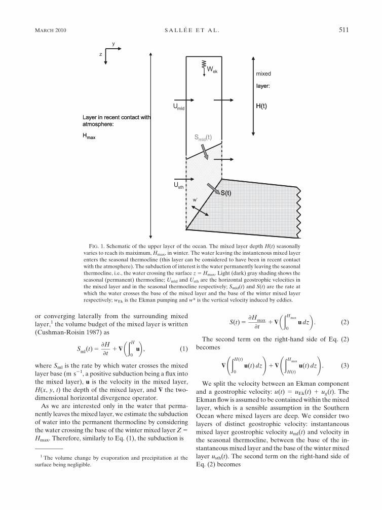
FIG. 1. Schematic of the upper layer of the ocean. The mixed layer depth H(t) seasonally
varies to reach its maiximum, Hmax, in winter. The water leaving the instantenous mixed layer
enters the seasonal thermocline (this layer can be considered to have been in recent contact
with the atmosphere). The subduction of interest is the water permanently leaving the seasonal
thermocline, i.e., the water crossing the surface z 5 Hmax. Light (dark) gray shading shows the
seasonal (permanent) thermocline; Umld and Usth are the horizontal geostrophic velocities in
the mixed layer and in the seasonal thermocline respectively; Smld(t) and S(t) are the rate at
which the water crosses the base of the mixed layer and the base of the winter mixed layer
respectively; wEk is the Ekman pumping and w* is the vertical velocity induced by eddies.
1 The volume change by evaporation and precipitation at the
surface being negligible.
MARCH 2010 S A L L E E E T A L . 511
ðHmax
0
u dz
� �5 $(U
Ek) 1 $(u
ml(t)H(t))
1 $[usth
(t)(Hmax� H(t))], (4)
where UEk is the Ekman transport. Exploiting the Argo
dataset, we resolve the seasonal cycle of the mixed layer
and examine the budget for monthly climatological means.
Since Hmax is fixed over the climatological annual cycle,
when averaged over a month Eq. (2) becomes
Sm
5 $(UEk
m) 1 $(u
ml(t)H(t)
m) 1 $(u
sth(t)(H
max�H(t))
m)
5 $(UEk
m) 1 $[(u
mlm 1 u
ml* )H
m] 1 $[(u
sthm 1 u
sth* )(H
max�H
m)],
(5)
where ( � )mdenotes a climatological monthly average,
(�)ml and (�)sth refer to mixed layer and seasonal thermo-
cline velocities, and u* the eddy-induced velocity (u* 5
u9H9m
/Hm
, see Gent and McWilliams 1990; see section
2.3 of McDougall 1991). Finally, assessing the divergence
of the geostrophic flow from the linear vorticity equation,
the monthly mean subduction through the base of the
winter mixed layer becomes
Sm
5 SEk
m1 S
geo
m1 S
eddy
m, (6a)
where
SEk
m5 w
Ekm, (6b)
Smgeo 5 u
mlm � $H
m1 u
sthm � $(H
max�H
m)
� b
f[H
my
mlm 1 (H
max�H
m) y
sthm], (6c)
and
Seddy
m5 $[u
ml* H
m1 u
sth* (H
max�H
m)]. (6d)
Annual mean subduction is the average of the monthly
means.
b. Transport in the upper ocean
As discussed above, subduction is the convergence of
water in the upper ocean (above the base of the winter
mixed layer). We examine the transport in the upper
ocean to understand better where the water subducted
into the ocean interior originates. We define the trans-
port above the winter mixed layer base to be
Tm
5
ðHmax
0
u(t) dz
� �m
5 UEk
m1 T
geo
m1 T
eddy
m, (7a)
where
Tgeo
m5 u
mlm H
m1 u
sthm (H
max�H
m) (7b)
and
Teddy
m5 u
ml* H
m1 u
sth* (H
max�H
m). (7c)
The buoyancy budget in the upper ocean is needed to
relate the transport to the diabatic processes of the up-
per ocean (e.g., Marshall 1997; Speer et al. 2000; Karsten
and Marshall 2002). The density of the water column
above Hmax (Fig. 1) can either be modified by air–sea
fluxes, lateral mixing and vertical diffusion, or by lateral
and vertical advection. Therefore, the transport of buoy-
ancy across a buoyancy surface b is (e.g., Marshall et al.
1999)
T(b)$b 5 Bsurf
(b) 1 Beddy
(b) 1 Bvertical
(b), (8)
where Bsurf is the air–sea buoyancy flux, Beddy the lateral
eddy buoyancy mixing above Hmax, and Bvertical the
vertical diffusion. We chose to set the vertical diffusion
to a constant value of kz 5 1.5 1025 m2 s21 [similar to,
e.g., Marshall et al. (1999), Karsten and Marshall (2002),
and to observations at the base of the mixed layer from
Cisewski et al. (2005)]. Then, one can easily relate the
subduction calculation to the buoyancy forcing (Bsurf 1
Beddy 1 Bvertical). We note that Eq. (8) is expressed in
terms of b, which undergoes a large seasonal cycle in the
mixed layer. We will therefore perform this calculation
in monthly averages, which will allow us to follow the
seasonal movement of b surfaces.
c. Eddy-induced velocity: u*
The water volume transport in a layer of thickness h
and velocity y is T 5 yh. Hence, the monthly mean av-
erage transport is
Tm
5 ym hm
1 y9h9m
, (9)
where the prime denotes an anomaly from the monthly
time average. Therefore, in addition to mixing, eddies
provide an advection of tracer by the eddy-induced ve-
locity defined here by
512 J O U R N A L O F P H Y S I C A L O C E A N O G R A P H Y VOLUME 40
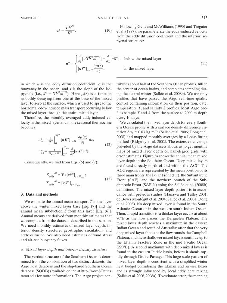
u* 5v9h9
m
hm . (10)
Following Gent and McWilliams (1990) and Treguier
et al. (1997), we parameterize the eddy-induced velocity
from the eddy diffusion coefficient and the interior iso-
pycnal structure:
u* 5
›
›z[k $b
m/b
z
m] 5
›
›z[k sm], below the mixed layer
[k sm]z5H
›m(z)
›z, in the mixed layer
8>><>>:
(11)
in which k is the eddy diffusion coefficient, b is the
buoyancy in the ocean, and s is the slope of the iso-
pycnals (i.e., sm 5 $bm
/bz
m). Here m(z) is a function
smoothly decaying from one at the base of the mixed
layer to zero at the surface, which is used to spread the
horizontal eddy-induced mass transport occurring below
the mixed layer through the entire mixed layer.
Therefore, the monthly averaged eddy-induced ve-
locity in the mixed layer and in the seasonal thermocline
becomes
uml* 5 1
Hm
ðHm
0
[k sm]z5H
›m(z)
›zdz,
usth* 5 1
Hmax�Hm
ðHmax
Hm
›
›z[k sm] dz.
(12)
Consequently, we find from Eqs. (6) and (7):
Seddy
m5 $ � [ksm]
z5Hmax;
Teddy
m5 [k sm]
z5Hmax.
(13)
3. Data and methods
We estimate the annual mean transport T in the layer
above the winter mixed layer base [Eq. (7)] and the
annual mean subduction S from this layer [Eq. (6)].
Annual means are derived from monthly estimates that
we compute from the datasets described in this section.
We need monthly estimates of mixed layer depth, in-
terior density structure, geostrophic circulation, and
eddy diffusion. We also need estimates of wind stress
and air–sea buoyancy fluxes.
a. Mixed layer depth and interior density structure
The vertical structure of the Southern Ocean is deter-
mined from the combination of two distinct datasets: the
Argo float database and the ship-based Southern Ocean
database (SODB) (available online at http://woceSOatlas.
tamu.edu for more information). The Argo project con-
tributes about half of the Southern Ocean profiles, fills in
the center of ocean basins, and completes sampling dur-
ing the austral winter (Sallee et al. 2008b). We use only
profiles that have passed the Argo real-time quality
control containing information on their position, date,
temperature T, and salinity S profiles. Most Argo pro-
files sample T and S from the surface to 2000-m depth
every 10 days.
We calculated the mixed layer depth for every South-
ern Ocean profile with a surface density difference cri-
terion Dsu # 0.03 kg m23 (Sallee et al. 2006; Dong et al.
2008) and mapped monthly averages by a Loess fitting
method (Ridgway et al. 2002). The extensive coverage
provided by the Argo datasets allows us to get monthly
maps of mixed layer depth on half-degree grids with
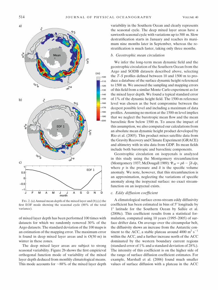
error estimates. Figure 2a shows the annual mean mixed
layer depth in the Southern Ocean. Deep mixed layers
are found directly north of and within the ACC. The
ACC regions are represented by the mean position of its
three main fronts: the Polar Front (PF), the Subantarctic
Front (SAF), and the northern branch of the Sub-
antarctic Front (SAF-N) using the Sallee et al. (2008b)
definitions. The mixed layer depth pattern is in accor-
dance with previous studies (Hanawa and Talley 2001;
de Boyer Montegut et al. 2004; Sallee et al. 2008a; Dong
et al. 2008). No deep mixed layer is found in the South
Atlantic Ocean or in the western south Indian Ocean.
Then, a rapid transition to a thicker layer occurs at about
708E as the flow passes the Kerguelen Plateau. The
mixed layer depth reaches a maximum in the eastern
Indian Ocean and south of Australia; after that the very
deep mixed layer shoals as the flow rounds the Campbell
Plateau, and these shallower mixed layers continue up to
the Eltanin Fracture Zone in the mid Pacific Ocean
(2208E). A second maximum with deep mixed layers is
found in the eastern Pacific basin, before it shoals rap-
idly through Drake Passage. This large-scale pattern of
mixed layer depth is consistent with a simplified winter
heat budget considering the Ekman and air–sea fluxes
and is strongly influenced by local eddy heat mixing
(Sallee et al. 2006, 2008a). To estimate error, the mapping
MARCH 2010 S A L L E E E T A L . 513
of mixed layer depth has been performed 100 times with
datasets for which we randomly removed 30% of the
Argo datasets. The standard deviation of the 100 maps is
an estimation of the mapping error. The maximum error
is found in deep mixed layer areas and is O(50 m) in
winter in these zones.
The deep mixed layer areas are subject to strong
seasonal variability. Figure 2b shows the first empiricval
orthogonal function mode of variability of the mixed
layer depth deduced from monthly climatological means.
This mode accounts for ;88% of the mixed layer depth
variability in the Southern Ocean and clearly represents
the seasonal cycle. The deep mixed layer areas have a
sawtooth seasonal cycle with variations up to 500 m. Slow
destratification starts in January and reaches its maxi-
mum nine months later in September, whereas the re-
stratification is much faster, taking only three months.
b. Geostrophic mean circulation
We infer the long-term mean dynamic field and the
geostrophic circulation of the Southern Ocean from the
Argo and SODB datasets described above, selecting
the T–S profiles defined between 10 and 1500 m to pro-
duce a database of the surface dynamic height referenced
to 1500 m. We assessed the sampling and mapping errors
of this field from a similar Monte Carlo experiment as for
the mixed layer depth. We found a typical standard error
of 1% of the dynamic height field. The 1500-m reference
level was chosen as the best compromise between the
deepest possible level and including a maximum of data
profiles. Assuming no motion at the 1500-m level implies
that we neglect the barotropic mean flow and the mean
baroclinic flow below 1500 m. To assess the impact of
this assumption, we also computed our calculations from
an absolute mean dynamic height product developed by
Rio et al. (2005). This product mixes satellite data from
the Gravity Recovery and Climate Experiment (GRACE)
and altimetry with in situ data from GDP. Its mean fields
include both barotropic and baroclinic components.
Geostrophic circulation on isopycnals is analyzed
in this study using the Montgomery streamfunction
(Montgomery 1937; McDougall 1989): CM 5 pd 2Ð
d dp,
where p is the pressure and d is the specific volume
anomaly. We note, however, that this streamfunction is
an approximation, neglecting the variations of specific
anomaly along the isopycnal surface: no exact stream-
function on an isopycnal exists.
c. Eddy diffusion coefficient
A climatological surface cross-stream eddy diffusivity
coefficient has been estimated in bins of 58 longitude by
18 latitude for the Southern Ocean by Sallee et al.
(2008c). This coefficient results from a statistical for-
mulation, computed using 10 years (1995–2005) of sur-
face drifter data. On average over the circumpolar belt,
the diffusivity shows an increase from the Antarctic con-
tinent to the ACC, a stable plateau around 4000 m2 s21
within the ACC, and a further increase north of the ACC
dominated by the western boundary current regions
(standard error of 1% and a standard deviation of 28%).
The intensity of this coefficient is on the higher side of
the range of surface diffusion coefficient estimates. For
example, Marshall et al. (2006) found much smaller
values of surface diffusion with a plateau in the ACC
FIG. 2. (a) Annual mean depth of the mixed layer and (b),(c) the
first EOF mode showing the seasonal cycle (88% of the total
variance).
514 J O U R N A L O F P H Y S I C A L O C E A N O G R A P H Y VOLUME 40
around 1000 m2 s21. The large range of diffusion coeffi-
cients estimates that exists in the literature comes from
the use of different methods. Indeed, studies resolving the
jets of the ACC have tended to show a reduction of the
surface diffusion coefficient in the ACC and an enhance-
ment at depth (Smith and Marshall 2009; Abernathey
et al. 2010; Naveira-Garabato et al. 2009, manuscript
submitted to J. Phys. Oceanogr.). Although Sallee et al.
(2008c) do not resolve the jets, they still represent the
only local estimates of a diffusion coefficient in the
Southern Ocean, and applying their coefficient with er-
ror bars is the best that we can do at present.
In addition, it has been shown that the high surface
diffusion coefficient better represents the mixing in a
coarse-resolution mixed layer model (Vivier et al. 2010).
Recent modeling studies suggest that surface intensified
diffusivity as large as 4000 m2 s21 improves the simula-
tion of the eddy-induced advection in the upper ocean
(Danabasoglu and Marshall 2007). Finally, Ferreira et al.
(2005) suggested that a high diffusion coefficient (up to
9000 m2 s21 at the surface) is needed in their coarse-
resolution residual mean ocean circulation model to min-
imize the departure from ocean observations. These
model studies at coarse resolution suggest that the ocean
surface is highly diffusive, in good agreement with Sallee
et al.’s (2008c) coefficient estimated on a coarse-resolution
grid. To better understand the impact of the choice of
mixing coefficient on the subduction and on the surface
layer transport, we will also use two others: one con-
stant surface value of 4000 m2 s21 as in Danabasoglu
and Marshall (2007) and one similar to that of Marshall
et al. (2006), that is, a constant value of 2000 m2 s21
outside the ACC and 1000 m2 s21 within the ACC. The
Marshall et al. coefficient is a circumpolar integrated
estimate, which suggests much lower surface diffusion
than Sallee et al. (2008c). Although an extension of their
study providing regional estimates of diffusion shows
closer values to Sallee et al. (2008c; see Shuckburgh et al.
2009), we will use the Marshall et al. coefficient to test
low coefficients.
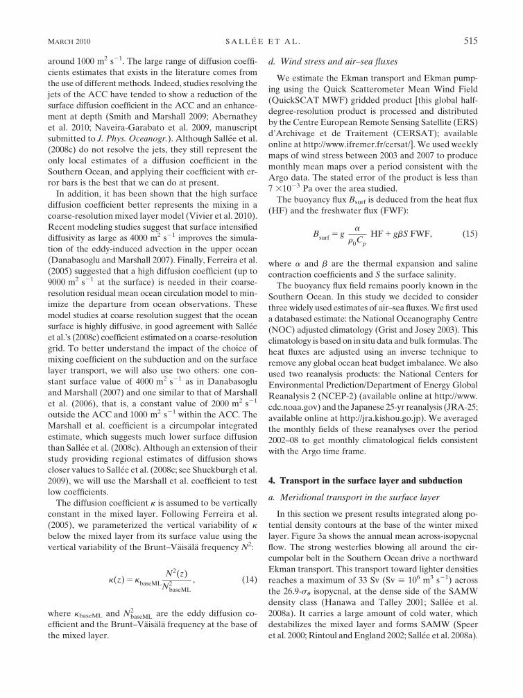
The diffusion coefficient k is assumed to be vertically
constant in the mixed layer. Following Ferreira et al.
(2005), we parameterized the vertical variability of k
below the mixed layer from its surface value using the
vertical variability of the Brunt–Vaisala frequency N2:
k(z) 5 kbaseML
N2(z)
N2baseML
, (14)
where kbaseML and N2baseML are the eddy diffusion co-
efficient and the Brunt–Vaisala frequency at the base of
the mixed layer.
d. Wind stress and air–sea fluxes
We estimate the Ekman transport and Ekman pump-
ing using the Quick Scatterometer Mean Wind Field
(QuickSCAT MWF) gridded product [this global half-
degree-resolution product is processed and distributed
by the Centre European Remote Sensing Satellite (ERS)
d’Archivage et de Traitement (CERSAT); available
online at http://www.ifremer.fr/cersat/]. We used weekly
maps of wind stress between 2003 and 2007 to produce
monthly mean maps over a period consistent with the
Argo data. The stated error of the product is less than
7 31023 Pa over the area studied.
The buoyancy flux Bsurf is deduced from the heat flux
(HF) and the freshwater flux (FWF):
Bsurf
5 ga
r0C
p
HF 1 gbS FWF, (15)
where a and b are the thermal expansion and saline
contraction coefficients and S the surface salinity.
The buoyancy flux field remains poorly known in the
Southern Ocean. In this study we decided to consider
three widely used estimates of air–sea fluxes. We first used
a databased estimate: the National Oceanography Centre
(NOC) adjusted climatology (Grist and Josey 2003). This
climatology is based on in situ data and bulk formulas. The
heat fluxes are adjusted using an inverse technique to
remove any global ocean heat budget imbalance. We also
used two reanalysis products: the National Centers for
Environmental Prediction/Department of Energy Global
Reanalysis 2 (NCEP-2) (available online at http://www.
cdc.noaa.gov) and the Japanese 25-yr reanalysis (JRA-25;
available online at http://jra.kishou.go.jp). We averaged
the monthly fields of these reanalyses over the period
2002–08 to get monthly climatological fields consistent
with the Argo time frame.
4. Transport in the surface layer and subduction
a. Meridional transport in the surface layer
In this section we present results integrated along po-
tential density contours at the base of the winter mixed
layer. Figure 3a shows the annual mean across-isopycnal
flow. The strong westerlies blowing all around the cir-
cumpolar belt in the Southern Ocean drive a northward
Ekman transport. This transport toward lighter densities
reaches a maximum of 33 Sv (Sv [ 106 m3 s21) across
the 26.9-su isopycnal, at the dense side of the SAMW
density class (Hanawa and Talley 2001; Sallee et al.
2008a). It carries a large amount of cold water, which
destabilizes the mixed layer and forms SAMW (Speer
et al. 2000; Rintoul and England 2002; Sallee et al. 2008a).
MARCH 2010 S A L L E E E T A L . 515
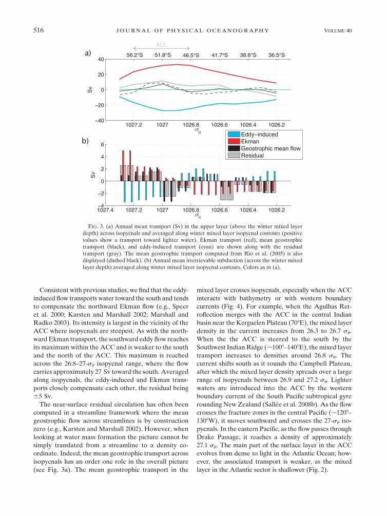
Consistent with previous studies, we find that the eddy-
induced flow transports water toward the south and tends
to compensate the northward Ekman flow (e.g., Speer
et al. 2000; Karsten and Marshall 2002; Marshall and
Radko 2003). Its intensity is largest in the vicinity of the
ACC where isopycnals are steepest. As with the north-
ward Ekman transport, the southward eddy flow reaches
its maximum within the ACC and is weaker to the south
and the north of the ACC. This maximum is reached
across the 26.8–27-su isopycnal range, where the flow
carries approximately 27 Sv toward the south. Averaged
along isopycnals, the eddy-induced and Ekman trans-
ports closely compensate each other, the residual being
65 Sv.
The near-surface residual circulation has often been
computed in a streamline framework where the mean
geostrophic flow across streamlines is by construction
zero (e.g., Karsten and Marshall 2002). However, when
looking at water mass formation the picture cannot be
simply translated from a streamline to a density co-
ordinate. Indeed, the mean geostrophic transport across
isopycnals has an order one role in the overall picture
(see Fig. 3a). The mean geostrophic transport in the
mixed layer crosses isopycnals, especially when the ACC
interacts with bathymetry or with western boundary
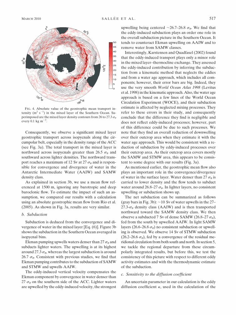
currents (Fig. 4). For example, when the Agulhas Ret-
roflection merges with the ACC in the central Indian
basin near the Kerguelen Plateau (708E), the mixed layer
density in the current increases from 26.3 to 26.7 su.
When the the ACC is steered to the south by the
Southwest Indian Ridge (;1008–1408E), the mixed layer
transport increases to densities around 26.8 su. The
current shifts south as it rounds the Campbell Plateau,
after which the mixed layer density spreads over a large
range of isopycnals between 26.9 and 27.2 su. Lighter
waters are introduced into the ACC by the western
boundary current of the South Pacific subtropical gyre
rounding New Zealand (Sallee et al. 2008b). As the flow
crosses the fracture zones in the central Pacific (;1208–
1308W), it moves southward and crosses the 27-su iso-
pycnals. In the eastern Pacific, as the flow passes through
Drake Passage, it reaches a density of approximately
27.1 su. The main part of the surface layer in the ACC
evolves from dense to light in the Atlantic Ocean; how-
ever, the associated transport is weaker, as the mixed
layer in the Atlantic sector is shallower (Fig. 2).
FIG. 3. (a) Annual mean transport (Sv) in the upper layer (above the winter mixed layer
depth) across isopycnals and averaged along winter mixed layer isopycnal contours (positive
values show a transport toward lighter water). Ekman transport (red), mean geostrophic
transport (black), and eddy-induced transport (cyan) are shown along with the residual
transport (gray). The mean geostrophic transport computed from Rio et al. (2005) is also
displayed (dashed black). (b) Annual mean irretrievable subduction (across the winter mixed
layer depth) averaged along winter mixed layer isopycnal contours. Colors as in (a).
516 J O U R N A L O F P H Y S I C A L O C E A N O G R A P H Y VOLUME 40
Consequently, we observe a significant mixed layer
geostrophic transport across isopycnals along the cir-
cumpolar belt, especially in the density range of the ACC
(see Fig. 3a). The total transport in the mixed layer is
northward across isopycnals greater than 26.5 su and
southward across lighter densities. The northward trans-
port reaches a maximum of 12 Sv at 27 su and is respon-
sible for convergence and divergence of water in the
Antarctic Intermediate Water (AAIW) and SAMW
density class.
As explained in section 3b, we use a mean flow ref-
erenced at 1500 m, ignoring any barotropic and deep
baroclonic flow. To estimate the impact of such an as-
sumption, we compared our results with a calculation
using an absolute geostrophic mean flow from Rio et al.
(2005). As shown in Fig. 3a, results are very similar.
b. Subduction
Subduction is deduced from the convergence and di-
vergence of water in the mixed layer [Eq. (6)]. Figure 3b
shows the subduction in the Southern Ocean averaged in
isopycnal bins.
Ekman pumping upwells waters denser than 27 su and
subducts lighter waters. The upwelling is at its highest
around 27.3 su, whereas the largest subduction is around
26.7 su. Consistent with previous studies, we find that
Ekman pumping contributes to the subduction of SAMW
and STMW and upwells AAIW.
The eddy-induced vertical velocity compensates the
Ekman component by convergence in water denser than
27 su on the southern side of the ACC. Lighter waters
are upwelled by the eddy-induced velocity, the strongest
upwelling being centered ;26.7–26.8 su. We find that
the eddy-induced subduction plays an order one role in
the overall subduction picture in the Southern Ocean. It
tends to counteract Ekman upwelling on AAIW and to
remove water from SAMW classes.
Interestingly, Karstensen and Quadfasel (2002) found
that the eddy-induced transport plays only a minor role
in the mixed layer–thermocline exchange. They assessed
the eddy-induced contribution by inferring the subduc-
tion from a kinematic method that neglects the eddies
and from a water age approach, which includes all com-
ponents; however, their error bars are big. Indeed, they
use the very smooth World Ocean Atlas 1998 (Levitus
et al. 1998) in the kinematic approach. Also, the water age
approach is based on a few lines of the World Ocean
Circulation Experiment (WOCE), and their subduction
estimate is affected by neglected mixing processes. They
refer to these errors in their study, and consequently
conclude that the difference they find is negligible and
does not reflect eddy-induced processes; however, part
of this difference could be due to such processes. We
note that they find an overall reduction of downwelling
over their outcrop area when they estimate it with the
water age approach. This would be consistent with a re-
duction of subduction by eddy-induced processes over
their outcrop area. As their outcrop area covers mostly
the SAMW and STMW area, this appears to be consis-
tent to some degree with our results (Fig. 3a).
As mentioned earlier, the geostrophic mean flow also
plays an important role in the convergence/divergence
of water in the surface layer. Water denser than 27 su is
carried to lower density and the flow tends to subduct
water around 26.8–27 su. In lighter layers, no consistent
upwelling or subduction shows up.
The net subduction can be summarized as follows
(gray bars in Fig. 3b): ;10 Sv of water upwells in the 27–
27.3-su density class (AAIW) and is then transported
northward toward the SAMW density class. We then
observe a subducted 7 Sv of dense SAMW (26.8–27 su),
fed from the south by upwelled AAIW. In light SAMW
layers (26.6–26.8 su) no consistent subduction or upwell-
ing is observed. We observe 14 Sv of STMW subduction
(26.2–26.6 su), fed by a convergence of the residual me-
ridional circulation from both south and north. In section 5,
we tackle the regional departure from these circum-
polarly integrated results, but before this, we test the
consistency of this picture with respect to different eddy
activity estimates and with the thermodynamic estimate
of the subduction.
c. Sensitivity to the diffusion coefficient
An uncertain parameter in our calculation is the eddy
diffusion coefficient k, used in the calculation of the
FIG. 4. Absolute value of the geostrophic mean transport in-
tensity (m2 s21) in the mixed layer of the Southern Ocean. Su-
perimposed are the mixed layer density contours from 26 to 27.3 su
every 0.1 kg m23.
MARCH 2010 S A L L E E E T A L . 517
eddy-induced flow. Recent observational studies have
provided different results concerning the magnitude of
the eddy diffusivity in the Southern Ocean (e.g., Marshall
et al. 2006; Sallee et al. 2008c; Shuckburgh et al. 2009). In
our study we chose to use the Lagrangian drifter-based
estimate from Sallee et al. (2008c). Here, we aim to quan-
tify the impact of this choice on the subduction picture. To
do so, we compute our calculations with two other surface
coefficients: one similar to the Marshall et al. (2006) es-
timate of average diffusivity, which is at the lower range of
diffusion estimates, and one similar to the constant co-
efficient from Danabasoglu and Marshall (2007).
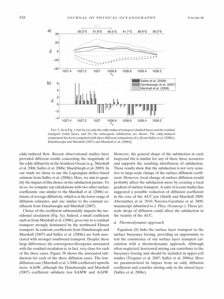
Choice of the coefficient substantially impacts the me-
ridional circulation (Fig. 5a). Indeed, a small coefficient
such as from Marshall et al. (2006), gives rise to a residual
transport strongly dominated by the northward Ekman
transport. In contrast, coefficients from Danabasoglu and
Marshall (2007) and Sallee et al. (2008c) are both asso-
ciated with stronger southward transport. Despite these
large differences, the convergence/divergence associated
with the residual circulation is, in fact, very close for each
of the three cases. Figure 5b shows the associated sub-
duction for each of the three diffusion cases. The low-
diffusion case (Marshall et al.’s 2006 coefficient) upwells
more AAIW, although the Danabasoglu and Marshall
(2007) coefficient subducts less SAMW and AAIW.
However, the general shape of the subduction in each
isopycnal bin is similar for any of these three scenarios
and supports the resulting distribution of subduction.
These results show that the subduction is not very sensi-
tive to large-scale change of the surface diffusion coeffi-
cient. However, local change of surface diffusion would
probably affect the subduction more by creating a local
gradient of surface transport. A suite of recent studies has
suggested a possible reduction of diffusion coefficient
in the core of the ACC jets (Smith and Marshall 2009;
Abernathey et al. 2010; Naveira-Garabato et al. 2009,
manuscript submitted to J. Phys. Oceanogr.). These jet-
scale drops of diffusion could affect the subduction in
the vicinity of the ACC.
d. Thermodynamic approach
Equation (8) links the surface layer transport to the
surface buoyancy forcing, providing an opportunity to
test the consistency of our surface layer transport cal-
culation with a thermodynamic approach. Although
often neglected, horizontal mixing can contribute to the
buoyancy forcing and should be included in upper-cell
studies (Treguier et al. 2007; Sallee et al. 2008a). Here
we parameterized its impact from an eddy diffusion
coefficient and consider mixing only in the mixed layer
(Sallee et al. 2008c).
FIG. 5. As in Fig. 3, but for (a) only the eddy-induced transport (dashed lines) and the residual
transport (solid lines), and (b) the subsequent subduction are shown. The eddy-induced
component has been computed with three different estimations of k: [from Sallee et al. (2008c),
Danabasoglu and Marshall (2007) and Marshall et al. (2006)].
518 J O U R N A L O F P H Y S I C A L O C E A N O G R A P H Y VOLUME 40
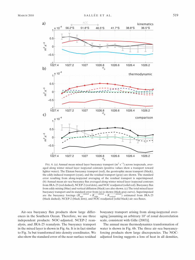
Air–sea buoyancy flux products show large differ-
ences in the Southern Ocean. Therefore, we use three
independent products: NOC-adjusted, NCEP-2 rean-
alysis, and JRA-25 reanalysis. The buoyancy transport
in the mixed layer is shown in Fig. 6a. It is in fact similar
to Fig. 3a but transformed into density coordinates. We
also show the standard error of the near-surface residual
bouyancy transport arising from along-isopycnal aver-
aging [assuming an arbitrary 108 of zonal decorrelation
scale, consistent with Gille (2003)].
The annual mean thermodynamics transformation of
water is shown in Fig. 6b. The three air–sea buoyancy-
forcing products show large discrepencies. The NOC-
adjusted forcing suggests a loss of heat in all densities,
FIG. 6. (a) Annual mean mixed layer buoyancy transport (m2 s23) across isopycnals, aver-
aged along winter mixed layer isopycnal contours (positive values show a transport toward
lighter water). The Ekman buoyancy transport (red), the geostrophic mean transport (black),
the eddy-induced transport (cyan), and the residual transport (gray) are shown. The standard
error resulting from along-isopycnal averaging of the residual transport is superimposed.
(b) Annual mean air–sea buoyancy flux averaged along winter mixed layer isopycnal contours
from JRA-25 (red dashed), NCEP-2 (red dots), and NOC readjusted (solid red). Buoyancy flux
from eddy mixing (blue) and vertical diffusion (black) are also shown. (c) The total mixed layer
buoyancy transport and its standard error from (a) is shown (thick-gray curve). Superimposed
are the buoyancy forcings (Bsurf
annual1 Beddy
annual1 Bvertical
annual) estimated from JRA-25
(black dashed), NCEP-2 (black dots), and NOC-readjusted (solid black) air–sea fluxes.
MARCH 2010 S A L L E E E T A L . 519
whereas the NCEP-2 suggests a gain of heat. Mixing
provides buoyancy on the light side of the strong gradients
(north) and extracts buoyancy on the dense side (south).
However, the averaging over the year, with isopycnal
meridionally moving owing to the mixed layer seasonal
cycle, tends to smooth out this frontal effect. We detect
a buoyancy gain signal on the dense side of the ACC
(around 27.2 su) and the western boundary currents
(around 26.4 su, Fig. 6b). Vertical diffusion has a negligi-
ble impact on the buoyancy. However, large uncertainties
remain on the vertical diffusion coefficient, and we note
that the vertical diffusion becomes significant in the
lightest density range when considering a coefficient kz
of O(1024 m2 s21).
The residual buoyancy forcing has a quite large en-
velope due to the discrepancy in the air–sea forcing
(Fig. 6c). However, a general shape is obtained, with
two maxima of buoyancy loss centered on 26.2 and
27.2 su. Although the thermodynamic and kinematics
results do not match exactly, they agree within the buoy-
ancy forcing envelope. We note that some inconsis-
tencies between the two approaches come from the
different ocean surface temperature used in the present
study and in the atmospheric reanalaysis products. A
comparison between the analyzed SST in JRA-25 and
the surface temperature from Argo floats suggests large
discrepencies, a maximum south of the ACC, around
27.3 su, where we consistently find the weakest agree-
ment between the thermodynamic and kinematic cal-
culations.
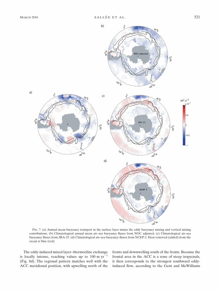
A qualitative regional comparison of the air–sea buoy-
ancy forcing and the buoyancy transport estimated from
the kinematic approach is presented in Fig. 7. We show
the buoyancy transport from which we removed the lat-
eral mixing by eddies and vertical diffusion (Tannual
$b
� Beddy
annual � Bvertical
annual, where ( � )annual
refers to
an annual mean carefully computed following the sea-
sonal cycle of the mixed layer density field) and we
compare it to the air–sea product (Bsurf
annual). We heavily
smoothed the results (over 58 of longitude and latitude)
to the typical spatial scale resolved by the reanalysis
products.
As above, we observed large discrepancies between
the three estimates of surface fluxes. However, these
three air–sea products show a large loss of buoyancy in
the western Indian Ocean and a small buoyancy gain or
reduced buoyancy loss in the Pacific basin. The air–sea
buoyancy fluxes needed to sustain our subduction cal-
culation thus show two key large-scale features. Our
results are qualitatively consistent with the three air–sea
products considered and imply realistic values of buoy-
ancy flux. The analysis shows that not all of the products
are necessarily in agreement.
5. Regional variability
a. Maps of subduction
The circumpolar integrated results presented above
suggest an overall upwelling of AAIW and downwelling
of dense SAMW. In this section, we investigate the re-
gional variability of the subduction and show that the
circumpolar integrated picture mixes regional regimes
and hides areas of intense subduction.
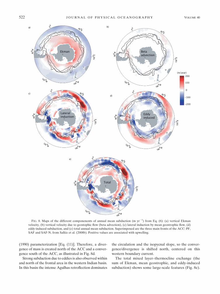
Ekman pumping has a near-zonal contribution to the
subduction with downwelling vertical velocity north of
the ACC and upwelling south of the ACC (Fig. 8a). This
is consistent with previous studies that showed the ACC
core position is related to a zero wind stress curl contour
(e.g., Chelton et al. 2004; Karstensen and Quadfasel 2002).
We divided the geostrophic contribution into two
pieces: the vertical velocity due to geostrophy [beta
advection term wz 5 (b/f ) yH] and the lateral induction
(u$H). The vertical velocity makes only a small contri-
bution to the subduction. The lateral induction term is
larger and induces velocities up to 200 m yr21. Strong
convergence is found in the Indian and Pacific western
basins where boundary currents flow southward and
merge with the ACC in the middle of the basins (near
Kerguelen at 708E and near the fracture zone at 2208E).
Before merging, these intense flows pass through a deep-
ening mixed layer in the subantarctic zone (see Fig. 2a),
which tends to bring water into the mixed layer (i.e., up-
welling).
Large areas of subduction are found in the subtropical
gyre, north of the western boundary currents, and north
of the ACC in the central and eastern basins. Figure 9a
shows the meridional mixed layer depth gradient along
with the surface geostrophic streamfunctions. North of
the intense currents, we observe branches of circulation
leaving the core of the ACC to circulate in the sub-
antarctic zone (especially near 608–708E, 1308E, and
1208–1408W). These branches flow through shoaling
mixed layers and consequently tend to push water out of
the mixed layer. Similarly, in Drake Passage the ACC
flows through a sharply shoaling mixed layer (Fig. 2),
which induces intense downwelling.
Large subduction is also observed where the ACC
shifts slightly toward the south away from the deep mixed
layer. For example, in the eastern Indian Ocean (around
1108E), the southeastern Indian Ridge steers the ACC to
flow southward across a mixed layer area, deepening to-
ward the north. Even if the southward shift is subtle, the
mixed layer gradient is sharp and the velocity is intense in
the ACC core; hence a large subduction is induced on the
southern edge of this deep mixed layer pool (Fig. 9).
Similar downwelling is observed as the ACC is steered
south in the eastern Pacific (around 1008W).
520 J O U R N A L O F P H Y S I C A L O C E A N O G R A P H Y VOLUME 40
The eddy-induced mixed layer–thermocline exchange
is locally intense, reaching values up to 100 m yr21
(Fig. 8d). The regional pattern matches well with the
ACC meridional position, with upwelling north of the
fronts and downwelling south of the fronts. Because the
frontal area in the ACC is a zone of steep isopycnals,
it then corresponds to the strongest southward eddy-
induced flow, according to the Gent and McWilliams
FIG. 7. (a) Annual mean buoyancy transport in the surface layer minus the eddy buoyancy mixing and vertical mixing
contributions. (b) Climatological annual mean air–sea buoyancy fluxes from NOC adjusted. (c) Climatological air–sea
buoyancy fluxes from JRA-25. (d) Climatological air–sea buoyancy fluxes from NCEP-2. Heat removed (added) from the
ocean is blue (red).
MARCH 2010 S A L L E E E T A L . 521
(1990) parameterization [Eq. (11)]. Therefore, a diver-
gence of mass is created north of the ACC and a conver-
gence south of the ACC, as illustrated in Fig. 8d.
Strong subduction due to eddies is also observed within
and north of the frontal area in the western Indian basin.
In this basin the intense Agulhas retroflection dominates
the circulation and the isopycnal slope, so the conver-
gence/divergence is shifted north, centered on this
western boundary current.
The total mixed layer–thermocline exchange (the
sum of Ekman, mean geostrophic, and eddy-induced
subduction) shows some large-scale features (Fig. 8e).
FIG. 8. Maps of the different componenents of annual mean subduction (m yr21) from Eq. (6): (a) vertical Ekman
velocity, (b) vertical velocity due to geostophic flow (beta advection), (c) lateral induction by mean geostrophic flow, (d)
eddy-induced subduction, and (e) total annual mean subduction. Superimposed are the three main fronts of the ACC: PF,
SAF and SAF-N, from Sallee et al. (2008b). Positive values are associated with upwelling.
522 J O U R N A L O F P H Y S I C A L O C E A N O G R A P H Y VOLUME 40
Large-scale upwellings, mainly due to lateral induction,
are observed in the western and central basins north of
the ACC in the Indian and Pacific Oceans. Elsewhere
north of the ACC, we observe several subduction areas
produced by lateral induction resulting from branches of
circulation leaving the ACC core. Strong downwelling
occurs when the ACC hits the shoaling mixed layer
around the Campbell Plateau (1708E) and in Drake
Passage. Lateral induction by geostrophic mean flow on
the southern edge of the deep mixed layer pool domi-
nates the mixed layer–thermocline exchanges in the
eastern Indian and Pacific basins (1208E and 908W).
Eddies dominate the subduction within the ACC core in
the western Indian basin and south of the ACC in the
Pacific basin. Finally, away from the ACC, Ekman
pumping dominates with downwelling water on the
northern side and upwelling water on the southern side.
We estimated the error associated with these up-
welling/downwelling structures from the datasets’ stated
errors and the mapping and sampling errors described in
section 3. We found median errors of 33 m yr21 for the
Ekman pumping, 27 m yr21 for the geostrophic mean
lateral induction, and 25 m yr21 for the eddy-induced
vertical velocity. This implies a total error of 85 m yr21
for the subduction, but the general structure of the
mixed layer–thermocline exchange remains within this
error limit and is fairly well defined.
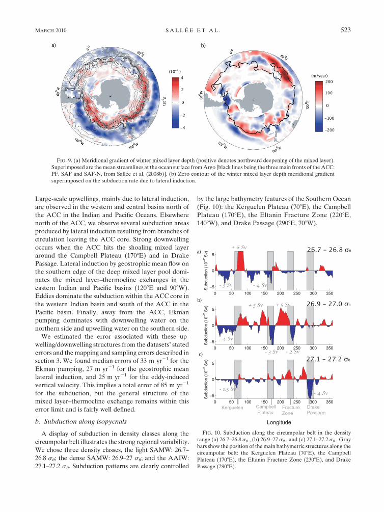
b. Subduction along isopycnals
A display of subduction in density classes along the
circumpolar belt illustrates the strong regional variability.
We chose three density classes, the light SAMW: 26.7–
26.8 su; the dense SAMW: 26.9–27 su; and the AAIW:
27.1–27.2 su. Subduction patterns are clearly controlled
by the large bathymetry features of the Southern Ocean
(Fig. 10): the Kerguelen Plateau (708E), the Campbell
Plateau (1708E), the Eltanin Fracture Zone (2208E,
1408W), and Drake Passage (2908E, 708W).
FIG. 9. (a) Meridional gradient of winter mixed layer depth (positive denotes northward deepening of the mixed layer).
Superimposed are the mean streamlines at the ocean surface from Argo [black lines being the three main fronts of the ACC:
PF, SAF and SAF-N, from Sallee et al. (2008b)]. (b) Zero contour of the winter mixed layer depth meridional gradient
superimposed on the subduction rate due to lateral induction.
FIG. 10. Subduction along the circumpolar belt in the density
range (a) 26.7–26.8 su , (b) 26.9–27 su , and (c) 27.1–27.2 su . Gray
bars show the position of the main bathymetric structures along the
circumpolar belt: the Kerguelen Plateau (708E), the Campbell
Plateau (1708E), the Eltanin Fracture Zone (2308E), and Drake
Passage (2908E).
MARCH 2010 S A L L E E E T A L . 523
Hotspots of subduction are found in the western In-
dian Ocean for the three density classes considered here.
These hotspots are dominated by an eddy-induced trans-
port convergence south of the intense Agulhas retroflec-
tion. Away from the western Indian Ocean, subduction in
each density class occurs at a preferred site. Whereas light
SAMWs downwells mostly in the eastern Indian Ocean
(;4 Sv, Fig. 10a), dense SAMWs subduct as the ACC
rounds the Campbell Plateau (;3 Sv, Fig. 10b) and
passes through the Eltanin Fracture Zone (;2 Sv, Fig.
10b). Consistent with previous studies, we find that the
AAIW density class water enters the permanent ther-
mocline mostly in Drake Passage (;4 Sv, Fig. 10c).
Near the Kerguelen Plateau light SAMW strongly
upwells (;6 Sv) into the mixed layer. The dense SAMW
upwells both in the eastern Indian Ocean (;5 Sv) and in
the western Pacific (;5 Sv). Because of these strong
upwelling regions, the net vertical velocity around the
circumpolar belt is positive (i.e., upwelling) in the SAMW
density class (Fig. 3b). However, this net upwelling is
actually composed of large downwelling and upwelling
variability. If the subducted water stays close to the base
of the mixed layer and is advected downstream, it is
likely to be reabsorbed by upwelling. In this situation,
the picture of the net mixed layer–thermocline exchange
is a good representation of the ventilation process.
However, if the subducted water is exported away from
the downwelling region by a circulation branch, then
each hotspot can ventilate the thermocline even if the
net mixed layer–thermocline exchange along the cir-
cumpolar belt shows no net subduction. The pathway of
particles in the interior needs to be taken into account in
studying the ventilation process. In the following we
tackle the issue of ventilated particle pathway, de-
scriptively, by examining tracers and circulation pat-
terns on density surfaces.
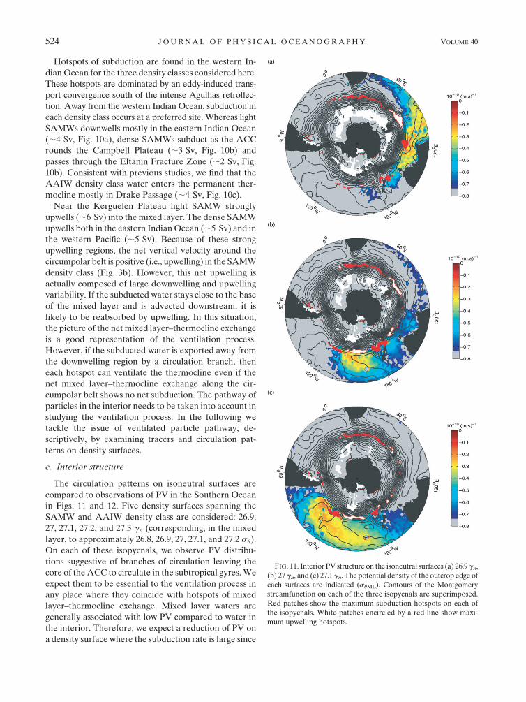
c. Interior structure
The circulation patterns on isoneutral surfaces are
compared to observations of PV in the Southern Ocean
in Figs. 11 and 12. Five density surfaces spanning the
SAMW and AAIW density class are considered: 26.9,
27, 27.1, 27.2, and 27.3 gn (corresponding, in the mixed
layer, to approximately 26.8, 26.9, 27, 27.1, and 27.2 su).
On each of these isopycnals, we observe PV distribu-
tions suggestive of branches of circulation leaving the
core of the ACC to circulate in the subtropical gyres. We
expect them to be essential to the ventilation process in
any place where they coincide with hotspots of mixed
layer–thermocline exchange. Mixed layer waters are
generally associated with low PV compared to water in
the interior. Therefore, we expect a reduction of PV on
a density surface where the subduction rate is large since
FIG. 11. Interior PV structure on the isoneutral surfaces (a) 26.9 gn,
(b) 27 gn, and (c) 27.1 gn. The potential density of the outcrop edge of
each surfaces are indicated (suML). Contours of the Montgomery
streamfunction on each of the three isopycnals are superimposed.
Red patches show the maximum subduction hotspots on each of
the isopycnals. White patches encircled by a red line show maxi-
mum upwelling hotspots.
524 J O U R N A L O F P H Y S I C A L O C E A N O G R A P H Y VOLUME 40
the interior is receiving large volumes of low PV water.
Water may also leave the mixed layer along more strat-
ified isopycnals; however, the rate is normally slower
since the isopycnal layers are thin.
The western Indian Ocean, south of Africa, is a region of
large mixed layer–thermocline exchanges in the SAMW
and AAIW density classes but with little consequence. In
this region, for each of the densities considered, water
subducts in the strong eastward flow of the ACC (red dots
south of Africa in Figs. 11 and 12). The water downwelled
in this region is not exported away from the base of
the mixed layer but this water is reabsorbed back into the
mixed layer in upwelling areas downstream, near the
Kerguelen Plateau.
The eastern Indian Ocean is a strong hotspot of sub-
duction in the 26.8 su (respectively, 26.9 gn). According
to Fig. 11, this hotspot coincides with flow toward the
subtropical gyre. Indeed, south of Australia, a branch of
circulation leaves the ACC core and loops back in the
eastern Indian Ocean to circulate in the south Indian
subtropical gyre. The PV structure is in good agreement
with these observations. First, we observe a strong re-
duction of PV right at the location of the subduction
hotspot, and second, the PV minimum created is ex-
ported away in the South Indian gyre through this ex-
change window. A smaller part is exported eastward.
The western Pacific Ocean is bounded by two sharp
bathymetric features: the Campbell Plateau and the
Eltanin Fracture Zone. As seen earlier, these two fea-
tures affected the subduction pattern on the isopycnals
26.9 and 27 su (respectively, 27 and 27.1 gn). Large
mass fluxes are found in the western Pacific south of
New Zealand on these two isopycnals (consistent with
Toggweiler et al. 1989). For both 26.9 su and 27 su, PV is
also strongly reduced near the Eltanin Fracture Zone. In-
deed, on 26.9 su there is a hotspot of downwelling slightly
to the west of the Eltanin Fracture Zone. A branch of
northward recirculation advects subducted water in a gyre
circulation. On 27 su the strong downwelling is slighly
shifted to the east. This subduction forms a minimum of
PV that is advected in the South Pacific subtropical gyre.
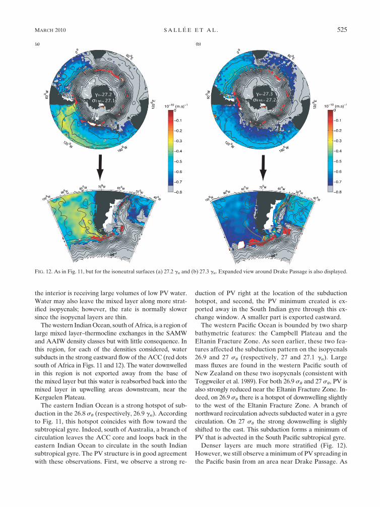
Denser layers are much more stratified (Fig. 12).
However, we still observe a minimum of PV spreading in
the Pacific basin from an area near Drake Passage. As
FIG. 12. As in Fig. 11, but for the isoneutral surfaces (a) 27.2 gn and (b) 27.3 gn. Expanded view around Drake Passage is also displayed.
MARCH 2010 S A L L E E E T A L . 525
seen earlier, Drake Passage is the location of a subdu-
ction maximum on these layers. Interestingly, the circu-
lation enters the area south of the tip of South America
and then comes back westward in the eastern Pacific,
advecting the low PV northward along the coast of Chile
before recirculating in the gyre. This is consistent with
previous studies that identified this branch of circulation
in AAIW layers from observational data (Suga and Talley
1995; Iudicone et al. 2007). The water entering Drake
Passage on the surface 27.2 su (27.3 gn) is very stratified
compared to lighter layers. However, we still observe
a slight reduction of PV. Similar to what happens on 27.1
su, a branch of circulation enters the region of large
subduction in Drake Passage and goes back into the
Pacific basin carrying ventilated water. Directly south of
the tip of South America a small closed gyrelike circula-
tion is observed, trapping water of very low PV. However,
most of the downwelling occurs in a strong eastward
current carrying the recently subducted water into the
Atlantic Ocean. We indeed observe a slightly lower PV in
the Atlantic basin on this layer.
6. Conclusions and discussion
The water mass exchange from the surface layer into
the interior has been estimated. The eddy-induced
transport in the surface layer makes a large contribution
to the transport, carrying ;30 Sv southward across the
ACC fronts. It tends to counterbalance the similarly
strong northward Ekman transport within the ACC
frontal system. The ACC surface geostrophic flow does
not strictly follow isopycnals along its circumpolar path.
The subsequent residual meridional circulation consists
of ;10 Sv of upwelling in the layer denser than 27 su,
which is advected toward the north in lighter layers.
Approximately 7 Sv are subducted into dense SAMW
(26.8–27 su), and no consistent downwelling or upwell-
ing is found in the lighter SAMWs (26.6–26.8 su). The
STMWs (26.2–26.6 su) are fed by northward residual
flows as well as by a southward flow, and a total of 14 Sv
are subducted in this layer.
This general structure of the mixed layer–thermocline
exchange is not very sensitive to large-scale change of
the diffusion coefficient and is consistent with existing
air–sea flux products. However, we found strong regional
variability, with downwelling and upwelling constrained
by bottom bathymetry. The bathymetry steers the circu-
lation, which affects the mixed layer depth distribution,
the circulation, and the slope of isopycnals—therefore
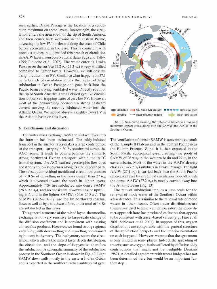
the subduction. A schematic summary of the subduction
process in the Southern Ocean is shown in Fig. 13. Light
SAMW downwells mostly in the eastern Indian Ocean
and is exported in the southern Indian subtropical gyre.
The ventilation of denser SAMW is concentrated south
of the Campbell Plateau and in the central Pacific near
the Eltanin Fracture Zone. It is then exported in the
South Pacific subtropical gyre, creating two pools of
SAMW of 26.9 su in the western basin and 27 su in the
eastern basin. Most of the water in the AAIW density
class (27.1–27.2 su) subducts in Drake Passage. The light
AAIW (27.1 su) is carried back into the South Pacific
subtropical gyre by a regional circulation loop, although
the dense AAIW (27.2 su) is mostly carried away into
the Atlantic Basin (Fig. 13).
The rate of subduction implies a time scale for the
renewal of mode water of the Southern Ocean within
a few decades. This is similar to the renewal rate of mode
waters in other oceans. Often tracer distributions are
themselves used to infer ventilation rates; the more di-
rect approach here has produced estimates that appear
to be consistent with tracer-based values (e.g., Fine et al.
2001; Schlosser et al. 2001). In support of this, oxygen
distributions are comparable with the general structure
of the subduction hotspots and the interior circulation
on each isopycnal. However, we note that the agreement
is only limited in some places. Indeed, the spreading of
tracers, such as oxygen, is also affected by diffusive eddy
contributions that might not be negligible (Jenkins
1987). A detailed agreement with tracer budgets has not
been determined here but would be an important fur-
ther step.
FIG. 13. Schematic showing the intense subduction areas and
maximum export areas, along with the SAMW and AAIW in the
Southern Ocean.
526 J O U R N A L O F P H Y S I C A L O C E A N O G R A P H Y VOLUME 40
Karsten and Marshall (2002) found a similar structure
of the meridional circulation: a meridional circulation
toward the north on the southern, dense side of the ACC
and toward the south on the northern, less-dense side.
However, they argued that the convergence is in AAIW
layers. In this study, we find, instead, the convergence in
the denser SAMW layers and also the STMW density
classes. Most importantly, we show that the circumpolar-
averaged structure hides regional variability and is not
representative of the local balances. Sloyan and Rintoul
(2001) also found that the northward Ekman transport is
largely compensated, suggesting that eddies play a ma-
jor role in the Southern Ocean meridional circulation.
They found a convergence of horizontal flow between
the STMW and the AAIW density class in the Atlantic
and Indian basin; however, they estimated a circumpolar
northward horizontal transport of 34 Sv in the AAIW,
which is more than the 12 Sv we find in this study. Marsh
et al. (2000) parameterized an eddy-induced transport in
their model and found a compensation of the northward
Ekman transport by eddies. Consistent with our find-
ings, the subduction they infer in their model is at its
maximum in the SAMW and is reduced toward the
AAIW density class. Finally, Lumpkin and Speer (2007)
estimated an upwelling in layers denser than 27 and a
subduction of SAMW water, using a global inverse
model, consistent with our results.
The estimates proposed in this study are a first step in
calculating the impact of eddies on the surface residual
circulation from observations. However, we consider only
the mesoscale and use a parameterization that could
be an inappropriate representation of the full complexity
of the mesoscale transport in the ocean (Hallberg and
Gnanadesikan 2006; Boning et al. 2008; Screen et al. 2009).
Recent studies have shown that smaller, submesoscale
eddies could have a great impact on the transfer between
the surface layer and interior ocean (Paci et al. 2005;
Lapeyre and Klein 2006; Thomas et al. 2010). Their role
as mixing processes or transport is not known. In addi-
tion, we neglected ventilation by diffusive processes at
the base of the mixed layer, which have an impact on
tracers (Joyce et al. 1998) and presumably affect the PV
flux, hence mass flux as well. A more complete under-
standing of these small scales and their role in the overall
meridional circulation structure would lead to a better
representation of the full ventilation process and a bet-
ter grasp of the impact of recent changes observed in the
Southern Ocean (Gille 2002; Morrow et al. 2008; Boning
et al. 2008).
Acknowledgments. Louise Bell kindly helped to draw
the schematic showing the intense areas of subduction. KS
received support from NSF OCE-0822075, OCE-0612167,
and OCE-0622670. JBS was supported by a CSIRO Office
of the Chief Executive (OCE) Postdoctoral Fellowship.
SR was supported by the Australian Government’s Co-
operative Research Centre’s Programme through the
Antarctic Climate and Ecosystems Cooperative Research
Centre (ACE-CRC). JBS, SR, and SW were also sup-
ported by the CSIRO Wealth from Oceans National
Research Flagship.
REFERENCES
Abernathey, R., J. Marshall, M. Mazloff, and E. Shuckburgh, 2010:
Enhancement of mesoscale eddy stirring at steering levels in
the Southern Ocean. J. Phys. Oceanogr., 40, 170–184.
Boning, C. W., A. Dispert, M. Visbeck, M. Rintoul, and
F. Schwarzkopf, 2008: Antarctic circumpolar current response
to recent climate change. Nat. Geosci., 1, 864–869.
Chelton, D. B., M. Schlax, M. Freilich, and R. Millif, 2004: Satellite
measurements reveal persistent small-scale features in ocean
winds. Science, 303, 978–983.
Cisewski, B., V. Strass, and H. Prandke, 2005: Upper-ocean vertical
mixing in the Antarctic Polar Front Zone. Deep-Sea Res. II,
52, 1087–1108.
Cushman-Roisin, B., 1987: Subduction. Dynamics of the Oceanic
Surface Mixed Layer: Proc. ‘Aha Huliko’a Hawaiian Winter
Workshop, Honolulu, HI, University of Hawaii at Manoa,
181–196.
Danabasoglu, G., and J. Marshall, 2007: Effects of vertical varia-
tions of thickness diffusivity in an ocean general circulation
model. Ocean Modell., 18, 122–141.
de Boyer Montegut, C., G. Madec, A. Fischer, A. Lazar, and
D. Iudicone, 2004: Mixed layer depth over the global
ocean: An examination of profile data and a profile-based
climatology. J. Geophys. Res., 109, C12003, doi:10.1029/
2004JC002378.
Dong, S., J. Sprintall, S. Gille, and L. Talley, 2008: Southern Ocean
mixed- layer depth from Argo float profiles. J. Geophys. Res.,
113, C06013, doi:10.1029/2006JC004051.
Ferreira, D., J. Marshall, and P. Heimbach, 2005: Estimating eddy
stresses by fitting dynamics to observations using a residual
mean ocean circulation model and its adjoint. J. Phys. Oce-
anogr., 35, 1891–1910.
Fine, R. A., K. A. Maillet, K. F. Sullivan, and D. Willey, 2001:
Circulation and ventilation flux of the Pacific Ocean. J. Geo-
phys. Res., 106 (C10), 22 159–22 178.
Follows, M. J., and J. C. Marshall, 1994: Eddy-driven exchange at
ocean fronts. Ocean Modell., 102, 5–9.
Gent, P., and J. McWilliams, 1990: Isopycnal mixing in ocean cir-
culation models. J. Phys. Oceanogr., 20, 150–155.
Gille, S. T., 2002: Warming of the Southern Ocean since the 1950s.
Science, 295, 1275–1277.
——, 2003: Float observations of the Southern Ocean. Part I: Esti-
mating mean fields, bottom velocities, and topographic steer-
ing. J. Phys. Oceanogr., 33, 1167–1181.
Grist, J. P., and S. A. Josey, 2003: Inverse analysis adjustment of the
SOC air–sea flux climatology using ocean heat transport
constraints. J. Climate, 16, 3274–3295.
Hallberg, R., and A. Gnanadesikan, 2006: The role of eddies in
determining the structure and response of the wind-driven
Southern Hemisphere overturning: Results from the Model-
ing Eddies in the Southern Ocean (MESO) Project. J. Phys.
Oceanogr., 36, 2232–2252.
MARCH 2010 S A L L E E E T A L . 527
Hanawa, K., and L. Talley, 2001: Mode waters. Ocean Circulation
and Climate, G. Siedler et al., Eds., International Geophysics
Series, Vol. 77, Academic Press, 373–386.
Huang, R. X., 1991: The three-dimensional structure of wind-driven
gyres: Ventilation and subduction. Rev. Geophys., 29 (Suppl.),
590–609.
Iudicone, D., K. Rodgers, R. Schopp, and G. Madec, 2007: An
exchange window for the injection of Antarctic Intermediate
Water into the South Pacific. J. Phys. Oceanogr., 37, 31–49.
Jenkins, W. J., 1982: On the climate of a subtropical gyre: Decadal
timescale variations in water mass renewal in the Sargasso Sea.
J. Mar. Res., 40, 265–290.
——, 1987: 3H and 3He in the Beta Triangle: Observations of gyre
ventilation and oxygen utilization rates. J. Phys. Oceanogr.,
17, 763–783.
Joyce, T. M., and W. J. Jenkins, 1993: Spatial variability of sub-
ducting water in the North Atlantic: A pilot study. J. Geophys.
Res., 98 (C6), 10 111–10 124.
——, J. R. Luyten, A. Kubryakov, F. B. Bahr, and J. S. Pallant,
1998: Meso- to large-scale structure of subducting water in the
subtropical gyre of the eastern North Atlantic Ocean. J. Phys.
Oceanogr., 28, 40–61.
Karsten, R., and J. Marshall, 2002: Constructing the residual cir-
culation of the ACC from observations. J. Phys. Oceanogr., 32,
3315–3327.
Karstensen, J., and D. Quadfasel, 2002: Formation of Southern
Hemisphere thermocline waters: Water mass conversion and
subduction. J. Phys. Oceanogr., 32, 3020–3038.
Lapeyre, G., and P. Klein, 2006: Dynamics of the upper oceanic
layers in terms of surface quasigeostrophic theory. J. Phys.
Oceanogr., 36, 165–176.
Ledwell, J., A. Watson, and C. Law, 1998: Mixing of a tracer in the
pycnocline. J. Geophys. Res., 103 (C10), 21 499–21 529.
Levitus, S., J. I. Antonov, T. P. Boyer, and C. Stephens, 1998:
Warming of the world. Ocean. Sci., 287, 2225–2229.
Lumpkin, R., and K. Speer, 2007: Global ocean meridional over-
turning. J. Phys. Oceanogr., 37, 2550–2562.
Luyten, J., J. Pedlosky, and H. Stommel, 1983: The ventilated
thermocline. J. Phys. Oceanogr., 13, 292–309.
Marsh, R., A. Nurser, A. Megann, and A. New, 2000: Water mass
formation in the Southern Ocean in a global isopycnal co-
ordinate GCM. J. Phys. Oceanogr., 30, 1013–1045.
Marshall, D., 1997: Subducting of water masses in an eddying
ocean. J. Mar. Res., 55, 201–222.
——, and J. Marshall, 1995: On the thermodynamics of subduction.
J. Phys. Oceanogr., 25, 138–151.
Marshall, J., and T. Radko, 2003: Residual mean solutions for the
Antarctic Circumpolar Current and its associated overturning
circulation. J. Phys. Oceanogr., 33, 2341–2354.
——, A. Nurser, and R. Williams, 1993: Inferring the subduction
rate and period over the North Atlantic. J. Phys. Oceanogr.,
23, 1315–1329.
——, D. Jamous, and J. Nilsson, 1999: Reconciling thermodynamic
and dynamic methods of computation of water mass trans-
formation rates. Deep-Sea Res. II, 46, 545–572.
——, H. Jones, R. Karsten, and R. Wardle, 2002: Can eddies set
ocean stratification? J. Phys. Oceanogr., 32, 26–38.
——, E. Shuckburgh, H. Jones, and C. Hill, 2006: Estimates and
implications of surface eddy diffusivity in the Southern
Ocean derived from tracer transport. J. Phys. Oceanogr., 36,
1806–1821.
McDougall, T. J., 1989: Streamfunctions for the lateral velocity
vector in a compressible ocean. J. Mar. Res., 47, 267–284.
——, 1991: Parameterizing mixing in inverse models. Dynamics of
Oceanic Internal Gravity Waves: Proc. Sixth. ‘Aha Huliko’a
Hawaiian Winter Workshop, P. Muller and D. Henderson,
Eds., Honolulu, HI, University of Hawaii at Manoa, 355–386.
Montgomery, R., 1937: A suggested method for representing gradient
flow in isentropic surfaces. Bull. Amer. Meteor. Soc., 18, 210.
Morrow, R., G. Valladeau, and J. Sallee, 2008: Observed sub-
surface signature of Southern Ocean decadal sea level rise.
Prog. Oceanogr., 77, 351–366.
Naveira-Garabato, A. C., J. Allen, H. Leach, V. Strass, and R. Pollard,
2001: Mesoscale subduction at the Antarctic Polar Front
driven by baroclinic instability. J. Phys. Oceanogr., 31, 2087–
2107.
Paci, A., G. Caniaux, M. Gavart, H. Giordani, M. Levy, L. Prieur, and
G. Reverdin, 2005: A high-resolution Simulation of the ocean
during the POMME experiment: Simulation results and com-
parison with observations. J. Geophys. Res., 110, doi:10.1029/
2004JC002712.
Qiu, B., and R. Huang, 1995: Ventilation of the North Atlantic and
North Pacific: Subduction versus obduction. J. Phys. Ocean-
ogr., 25, 2374–2390.
Rhines, P. B., and W. R. Young, 1982: Homogenization of potential
vorticity in planetary gyres. J. Fluid Mech., 122, 347–367.
Ridgway, K., J. Dunn, and J. Wilkin, 2002: Ocean interpolation by
four-dimensional weighted least squares—Application to the
waters around Australasia. J. Atmos. Oceanic Technol., 19,
1357–1375.
Rintoul, S., and M. England, 2002: Ekman transport dominates air–
sea fluxes in driving variability of subantarctic mode water. J.
Phys. Oceanogr., 32, 1308–1321.
Rio, M., P. Schaeffer, F. Hernandez, and J. Lemoine, 2005: The es-
timation of the ocean mean dynamic topography through the
combination of altimetric data, in-situ measurements and
GRACE geoid: From global to regional studies. Proc. GOCINA
Int. Workshop, Luxembourg, Geoid and Ocean Circulation in
the North Atlantic, 171–177.
Robbins, P. E., J. Price, W. B. Owens, and W. Jenkins, 2000: The
importance of lateral diffusion for the ventilation of the lower
thermocline in the subtropical North Atlantic. J. Phys. Oce-
anogr., 30, 67–89.
Robinson, A. R., and H. Stommel, 1959: The oceanic thermo-
cline and the associated thermohaline circulation. Tellus, 11,
295–308.
Rupolo, V., 2007: A Lagrangian-based approach for determining
trajectories taxonomy and turbulence regimes. J. Phys. Oce-
anogr., 37, 1584–1609.
Sallee, J., N. Wienders, R. Morrow, and K. Speer, 2006: Forma-
tion of Subantarctic Mode Water in the southeastern Indian
Ocean. Ocean Dyn., 56, 525–542, doi:10.1007/s10236-005-
0054-x.
——, R. Morrow, and K. Speer, 2008a: Eddy diffusion and Sub-
antarctic Mode Water formation. Geophys. Res. Lett., 35,
L05607, doi:10.1029/2007GL032827.
——, K. Speer, and R. Morrow, 2008b: Response of the Antarctic
Circumpolar Current to atmospheric variability. J. Climate, 21,
3020–3039.
——, ——, ——, and R. Lumpkin, 2008c: An estimate of La-
grangian eddy statistics and diffusion in the mixed layer of the
Southern Ocean. J. Mar. Res., 66, 441–463.
Sarmiento, J., 1983: A tritium box model of the North Atlantic
thermocline. J. Phys. Oceanogr., 13, 1269–1274.
Schlosser, P., J. Bullister, R. Fine, W. Jenkins, R. Key, J. Lupton,
W. Roether, and W. Smethie, 2001: Transformation and age of
528 J O U R N A L O F P H Y S I C A L O C E A N O G R A P H Y VOLUME 40
water masses. Ocean Circulation and Climate: Observing and
Modelling the Global Ocean, G. Siedler et al., Eds., International
Geophysics Series, Vol. 77, Academic Press, 427–450.
Screen, J., N. Gillett, D. Stevens, G. Marshall, and H. Roscoe, 2009:
The role of eddies in the Southern Ocean tempereature re-
sponse to the Southern Annular Mode. J. Climate, 22, 806–818.
Shuckburgh, E., E. Jones, J. Marshall, and C. Hill, 2009: Under-
standing the regional variability of eddy diffusivity in the Pacific
sector of the Southern Ocean. J. Phys. Oceanogr., 39, 2011–2023.
Sloyan, B., and S. Rintoul, 2001: Circulation, renewal, and modi-
fication of Antarctic Mode Water and Intermediate Water.
J. Phys. Oceanogr., 31, 1005–1030.
Smith, K. S., and J. Marshall, 2009: Evidence for deep eddy mixing
in the Southern Ocean. J. Phys. Oceanogr., 39, 50–69.
Sorensen, J., J. Ribbe, and G. Shaffer, 2001: On Antarctic Inter-
mediate Water mass formation in general circulation models.
J. Phys. Oceanogr., 31, 77–91.
Speer, K., and E. Tziperman, 1992: Rates of water mass formation
in the North Atlantic Ocean. J. Phys. Oceanogr., 22, 93–104.
——, S. R. Rintoul, and B. M. Sloyan, 2000: The diabatic Deacon
cell. J. Phys. Oceanogr., 30, 3212–3222.
Suga, T., and L. D. Talley, 1995: Antarctic Intermediate Water
circulation in the tropical and subtropical South Atlantic.
J. Geophys. Res., 100 (C7), 13 441–13 453.
Sundermeyer, M. A., and J. Price, 1998: Lateral mixing and the
North Atlantic Tracer Release Experiment: Observations and
numerical simulations of Lagrangian particles and a passive
tracer. J. Geophys. Res., 103 (C10), 21 481–21 497.
Thomas, L., C. Lee, and Y. Yoshikawa, 2010: The subpolar Front
of the Japan/East Sea. Part II: Inverse method for de-
termining the frontal vertical circulation. J. Phys. Oceanogr.,
40, 3–25.
Toggweiler, J. R., K. Dixon, and K. Bryan, 1989: Simulations of
radiocarbon in a coarse-resolution World Ocean Model. 2.
Distributions of bomb-produced carbon 14. J. Geophys. Res.,
94 (C6), 8243–8264.
Treguier, A., I. Held, and V. Larichev, 1997: Parameterization of
quasigeostrophic eddies in primitive equation ocean model.
J. Phys. Oceanogr., 27, 567–580.
——, M. England, S. Rintoul, G. Madec, J. Le Sommer, and
J. Molines, 2007: Upper-ocean meridional circulation in a nu-
merical model of the Antarctic Circumpolar Current. Ocean
Sci., 4, 653–698.
Vivier, F., D. Iudicone, F. Busdraghi, and Y.-H. Park, 2010: Dy-
namics of sea surface temperature anomalies in the Southern
Ocean diagnosed from a 2-D mixed layer model. Ocean Mod-
ell., 40, 3–25.
Welander, P., 1959: An advective model of the ocean thermocline.
Tellus, 11, 309–318.
Woods, J. D., 1985: The physics of thermocline ventilation. Cou-
pled Ocean–Atmosphere Models, J. C. J. Nihoul, Ed., Elsevier
Oceanography Series, Vol. 40, Elsevier, 543–590.
Zhurbas, V., and I. Oh, 2004: Drifter-derived maps of lateral dif-
fusivity in the Pacific and Atlantic Oceans in relation to sur-
face circulation patterns. J. Geophys. Res., 109, C05015,
doi:10.1029/2003JC002241.
MARCH 2010 S A L L E E E T A L . 529


![Nonbreaking wave‐induced mixing in upper ocean during ... · layer by entraining cooler water from the thermocline up into the well-mixed ocean surface [Yablonsky et al., 2015a]](https://static.cupdf.com/doc/110x72/602546ee425f8f53b55e6217/nonbreaking-waveainduced-mixing-in-upper-ocean-during-layer-by-entraining.jpg)