Reactive AUV motion for thermocline tracking

Reactive AUV Motion forThermocline Tracking

Nuno A. Cruz and Anı́bal C. MatosINESC Porto and FEUP–DEEC

Rua Dr. Roberto Frias, 378; 4200-465 Porto; PortugalEmail: {nacruz, anibal}@fe.up.pt

Abstract— The thermocline is a vertical transition layer in thewater column with a strong impact on marine biology, since itaffects phytoplankton concentration and, hence, primary pro-duction. AUVs can play an important role in understanding thisrelationship, by sampling the relevant data, usually describingyo-yo patterns spanning the whole water column. In this paperwe describe a reactive behavior implemented onboard a smallsized AUV, to adapt depth in real time in order to maintain thevehicle in the vicinity of the thermocline and therefore increasingefficiency in the sampling process. Preliminary field tests showthat the method is simple, robust and effective.

I. INTRODUCTION

Autonomous Underwater Vehicles (AUVs) are extremelyversatile platforms to sample wide regions of underwaterenvironments with minimal setup and operational costs. Inmost current applications, AUVs are programmed to followgeo-referenced paths while collecting relevant data, whichyields more efficient synoptic views of 3D fields as comparedto traditional ocean sampling techniques. However, if themission objective concerns the search for a given underwaterfeature, then the pre-programmed path has to include all theregions where the feature is likely to be found, resulting ina small percentage of useful data about the specific feature.More, it is common for this data to be post-processed off-lineby a human operator to refine the mission plan, which takesvaluable time and may even prevent the re-acquisition of adynamic feature.

A standard AUV navigation system is based on a kinematicor dynamic model that relates the vehicle actuation with thestate variables that are used in the feedback loops (positionand velocity). All relevant sensors to map the underwaterfeatures are carried as independent payload sensors, withno direct influence on vehicle control or navigation. CurrentAUV implementations carry tremendous on-board computa-tional power, which allows for real time, on-line processingof data being collected. As a consequence, it is possible toimplement algorithms for AUV guidance that take into accountinformation extracted from a given feature being mapped inorder to increase the efficiency in the observation procedure ofthat same feature, in a process frequently known as adaptivesampling. This requires a careful design of the AUV on-boardnavigation system so that the motion characteristics of thevehicle may be modified in real time without compromisingsafety and robustness. The main difficulty for this approach isthe absence of simple models that relate the mapped features

with the vehicle dynamics. Even if feature models are knownor assumed, their specific parameters have to be estimated inreal time using discrete, possibly noisy measurements.

Our strategy relies on relatively simple feature models forwhich the AUV can estimate relevant parameters in real time,and then use these parameters to define the motion characteris-tics (and sampling pattern) of the AUV. This way, the AUV isable to decide an adequate trajectory in order to concentrate themeasurements in the region of interest, yielding a significantimprovement in efficiency as compared to a standard broadsurvey. Some other forms of reactive behaviors have alreadybeen implemented with success in AUVs, particularly for thecase of finding the sources of chemical plumes, most of themtrying to mimic the real behavior of lobsters or bacterium inodor source localization ([1]–[3]).

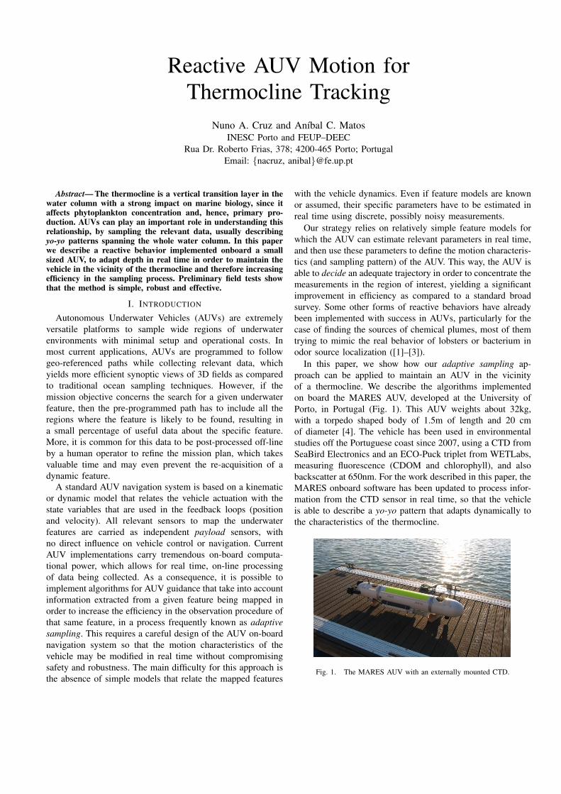
In this paper, we show how our adaptive sampling ap-proach can be applied to maintain an AUV in the vicinityof a thermocline. We describe the algorithms implementedon board the MARES AUV, developed at the University ofPorto, in Portugal (Fig. 1). This AUV weights about 32kg,with a torpedo shaped body of 1.5m of length and 20 cmof diameter [4]. The vehicle has been used in environmentalstudies off the Portuguese coast since 2007, using a CTD fromSeaBird Electronics and an ECO-Puck triplet from WETLabs,measuring fluorescence (CDOM and chlorophyll), and alsobackscatter at 650nm. For the work described in this paper, theMARES onboard software has been updated to process infor-mation from the CTD sensor in real time, so that the vehicleis able to describe a yo-yo pattern that adapts dynamically tothe characteristics of the thermocline.

Fig. 1. The MARES AUV with an externally mounted CTD.

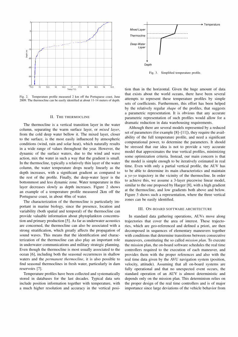
Fig. 2. Temperature profile measured 2 km off the Portuguese coast, June2009. The thermocline can be easily identified at about 11-14 meters of depth.

II. THE THERMOCLINE

The thermocline is a vertical transition layer in the watercolumn, separating the warm surface layer, or mixed layer,from the cold deep water bellow it. The mixed layer, closerto the surface, is the most easily influenced by atmosphericconditions (wind, rain and solar heat), which naturally resultsin a wide range of values throughout the year. However, thedynamic of the surface waters, due to the wind and waveaction, mix the water in such a way that the gradient is small.In the thermocline, typically a relatively thin layer of the watercolumn, the water temperature drops nearly linearly as thedepth increases, with a significant gradient as compared tothe rest of the profile. Finally, the deep-water layer is thebottommost and less dynamic zone. Water temperature in thislayer decreases slowly as depth increases. Figure 2 showsan example of a temperature profile measured 2km off thePortuguese coast, in about 40m of water.

The characterization of the thermocline is particularly im-portant in marine biology, since the presence, location andvariability (both spatial and temporal) of the thermocline canprovide valuable information about phytoplankton concentra-tion and primary production [5]. As far as underwater acousticsare concerned, the thermocline can also be associated with astrong stratification, which greatly affects the propagation ofsound waves. This means that the identification and charac-terization of the thermocline can also play an important rolein underwater communications and military strategic planning.Even though the thermocline is most usually associated to theocean [6], including both the seasonal occurrences in shallowwaters and the permanent thermocline, it is also possible tofind seasonal thermoclines in fresh water, particularly in damreservoirs [7].

Temperature profiles have been collected and systematicallystored in databases for the last decades. Typical data setsinclude position information together with temperature, witha much higher resolution and accuracy in the vertical posi-

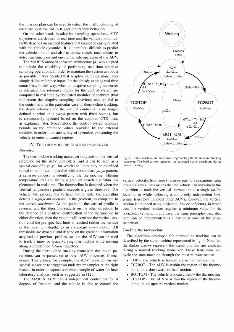
Fig. 3. Simplified temperature profile.

tion than in the horizontal. Given the huge amount of datathat exists about the world oceans, there have been severalattempts to represent these temperature profiles by simplesets of coefficients. Furthermore, this effort has been helpedby the relatively regular shape of the profiles, that suggestsa parametric representation. It is obvious that any accurateparametric representation of such profiles would allow for adramatic reduction in data warehousing requirements.

Although there are several models represented by a reducedset of parameters (for example [8]–[11]), they require the avail-ability of the full temperature profile, and need a significantcomputational power, to determine the parameters. It shouldbe stressed that our idea is not to provide a very accuratemodel that approximates the true vertical profiles, minimizingsome optimization criteria. Instead, our main concern is thatthe model is simple enough to be iteratively estimated in realtime. Even with only a partial vertical profile, the AUV hasto be able to determine its main characteristics and maintaina yo-yo trajectory in the vicinity of the thermocline. In orderto achieve this, we assume a 3-layer piecewise linear model,similar to the one proposed by Haeger [8], with a high gradientat the thermocline, and low gradients both above and below.Figure 3 shows such a representation, where the three verticalzones can be easily identified.

III. ON-BOARD SOFTWARE ARCHITECTURE

In standard data gathering operations, AUVs move alongtrajectories that cover the area of interest. These trajecto-ries, which are geo-referenced and defined a priori, are thendecomposed in sequences of elementary maneuvers togetherwith conditions that determine transitions between consecutivemaneuvers, constituting the so called mission plan. To executethe mission plan, the on-board software schedules the real timecontrollers required to the execution of each maneuver, andprovides them with the proper references and also with thereal time data given by the AVU navigation system (position,velocity, attitude). Assuming that all on-board systems arefully operational and that no unexpected event occurs, thestandard operation of an AUV is almost deterministic anddepends only on the mission plan. This determinism relies onthe proper design of the real time controllers and is of majorimportance since large deviations of the vehicle behavior from

the mission plan can be used to detect the malfunctioning ofon-board systems and to trigger emergency behaviors.

On the other hand, in adaptive sampling operations, AUVtrajectories are defined in real time and the vehicle motion di-rectly depends on mapped features that cannot be easily relatedwith the vehicle dynamics. It is, therefore, difficult to predictthe vehicle motion and also to devise simple mechanisms todetect malfunctions and ensure the safe operation of the AUV.

The MARES onboard software architecture [4] was adaptedto include the capability of performing real time adaptivesampling operations. In order to maintain the system as robustas possible it was decided that adaptive sampling maneuverssimply define reference inputs for the already existing real timecontrollers. In this way, when an adaptive sampling maneuveris activated, the reference inputs for the control system arecomputed in real time by dedicated modules of software (thatimplement the adaptive sampling behaviors) and are fed tothe controllers. In the particular case of thermocline tracking,the depth reference for the vertical controller is no longerdefined a priori in a yo-yo pattern with fixed bounds, butis continuously updated based on the acquired CTD data,as explained later. Nonetheless, the control system imposesbounds on the reference values provided by the externalmodules in order to ensure safety of operation, preventing thevehicle to enter unwanted regions.

IV. THE THERMOCLINE TRACKING MANEUVER

Overview

The thermocline tracking maneuver only acts on the verticalreference for the AUV controllers, and it can be seen as aspecial case of a yo-yo, for which the limits may be redefinedin real time. In fact, in parallel with the standard yo-yo pattern,a separate process is identifying the thermocline, filteringtemperature data and fitting a gradient search algorithm im-plemented in real time. The thermocline is detected when thevertical temperature gradient exceeds a given threshold. Thevehicle will proceed the vertical motion until the algorithmdetects a significant decrease in the gradient, as compared tothe current maximum. At this position, the vertical profile isreversed and the algorithm restarts on the other direction. Inthe absence of a positive identification of the thermocline ineither direction, then the vehicle will continue the vertical mo-tion until the pre-specified limit is reached (either the surfaceor the maximum depth), as in a standard yo-yo motion. Allthresholds are dynamic and depend on the gradient informationacquired on previous profiles, so that the AUV can be usedto track a time- or space-varying thermocline while movingalong a pre-defined lat-lon trajectory.

During the thermocline tracking maneuver, the model pa-rameters can be passed on to other AUV processes, if nec-essary. This allows, for example, the AUV to switch on anyspecial sensor or to trigger an underwater sampler at the rightinstant, in order to capture a relevant sample of water for laterlaboratory analysis, such as suggested in [12].

The MARES AUV has 4 independent controllers for 4degrees of freedom, and the vehicle is able to control the

Fig. 4. State machine and transitions representing the thermocline trackingmaneuver. The bold arrows represent the expected cyclic transitions duringnormal tracking.

vertical velocity, from zero (i.e. hovering) to a maximum valuearound 40cm/s. This means that the vehicle can implement thisalgorithm to track the vertical thermocline at a single lat-lonlocation, or while following a completely independent hori-zontal trajectory. In most other AUVs, however, the verticalmotion is obtained using horizontal fins or deflectors, in whichcase the vertical motion requires a minimum value for thehorizontal velocity. In any case, the same principles describedhere can be implemented as a particular case of the yo-yomaneuver.

Tracking the thermocline

The algorithm developed for thermocline tracking can bedescribed by the state machine represented in fig. 4. Note thatthe darker arrows represent the transitions that are expectedduring a normal tracking maneuver. These transitions willcycle the state machine through the most relevant states:

• TOP - The vehicle is located above the thermocline.• TC2BOT - The AUV is within the region of the thermo-

cline, on a downward vertical motion.• BOTTOM - The vehicle is located below the thermocline.• TC2TOP - The AUV is within the region of the thermo-

cline, on an upward vertical motion.

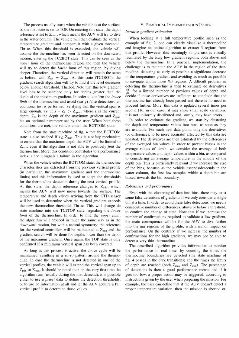
The process usually starts when the vehicle is at the surface,so the first state is set to TOP. On entering this state, the depthreference is set to Zmax, which means the AUV will try to divein the water column. The vehicle will then evaluate the verticaltemperature gradient and compare it with a given threshold,Thr tc. When this threshold is exceeded, the vehicle willassume the thermocline has been detected on the downwardmotion, entering the TC2BOT state. This can be seen as theupper limit of the thermocline region and then the vehiclewill try to detect the lower limit of this region, by divingdeeper. Therefore, the vertical direction will remain the sameas before, with Zref = Zmax. At this state (TC2BOT), thegradient search algorithm will try to find if the level decreasesbelow another threshold, Thr bot. Note that this low gradientlevel has to be searched only for depths greater than thedepth of the maximum gradient. In order to confirm the lowerlimit of the thermocline and avoid (early) false detections, anadditional test is performed, verifying that the vertical span islarge enough, i.e. if z − Ztc > Zspan, where z is the currentdepth, Ztc is the depth of the maximum gradient and Zspanhis an optional parameter set by the user. When both theseconditions are met, the vehicle enters the BOTTOM state.

Note from the state machine of fig. 4 that the BOTTOMstate is also reached if z≥ Zmax. This is a safety mechanismto ensure that the maximum depth the AUV will be limited toZmax, even if the algorithm is not able to positively find thethermocline. More, this condition contributes to a performanceindex, since it signals a failure in the algorithm.

When the vehicle enters the BOTTOM state, the thermoclinecharacteristics are extracted from the previous vertical profile(in particular, the maximum gradient and the thermoclinelimits) and this information is used to adapt the thresholdsfor the thermocline detection during the next vertical profile.At this state, the depth reference changes to Zmin, whichmeans the AUV will now move towards the surface. Thetemperature and depth values arriving from the CTD sensorwill be used to determine when the vertical gradient exceedsthe new thermocline threshold, Thr tc. This will change destate machine into the TC2TOP state, signaling the lowerlimit of the thermocline. In order to find the upper limit,the algorithm will proceed in much the same way as in thedownward motion, but with a natural symmetry: the referencefor the vertical controllers will be maintained at Zmin and thegradient search will be done for depths lower than the depthof the maximum gradient. Once again, the TOP state is onlyconfirmed if a minimum vertical span has been covered.

As long as this process is active, the above cycle will bemaintained, resulting in a yo-yo pattern around the thermo-cline. In case the thermocline is not detected in one of thevertical profiles, the vehicle will extend the vertical span up toZmin or Zmax. It should be noted than on the very first time thealgorithm runs (usually during the first descend), it is possibleeither to use a priori data to define the detection thresholds,or to use no information at all and let the AUV acquire a fullvertical profile to determine those values.

V. PRACTICAL IMPLEMENTATION ISSUES

Iterative gradient estimation

When looking at a full temperature profile such as theexample of fig. 2, one can clearly visualize a thermoclineand imagine an online algorithm to extract 3 regions fromthat profile. However, this seemingly simple task is visuallyfacilitated by the long low gradient regions, both above andbelow the thermocline. In a practical implementation, thechallenge is to maintain the AUV in the region of the ther-mocline, detecting as early as possible a significant decreasein the temperature gradient and avoiding as much as possibleto navigate within those flat regions. A difficult problem indetecting the thermocline is then to estimate de derivativesdTdz for a limited number of previous values of depth anddecide if those derivatives are sufficient to conclude that thethermocline has already been passed and there is no need toproceed further. More, this data is updated several times persecond (16, in our case), it may show small scale variations,it is not uniformly distributed and, surely, may have errors.

In order to estimate the gradient, we start by clusteringthe depth and temperature values into bins, as soon as theyare available. For each new data point, only the derivatives(or differences, to be more accurate) affected by this data areupdated. The derivatives are then estimated by the differencesof the averaged bin values. In order to prevent biases in theaverage values of depth, we consider the average of bothtemperature values and depth values within a bin, as comparedto considering an average temperature in the middle of thedepth bin. This is particularly relevant if we increase the sizeof the bins, because as the vehicle ascends/descends in thewater column, the first few samples within a depth bin arebiased towards the bin boundary.

Robustness and performance

Even with the clustering of data into bins, there may existsome false detections of gradients if we only consider a singlebin at a time. In order to avoid these false detections, we need aconsecutive number of differences, above or below a threshold,to confirm the change of state. Note that if we increase thenumber of confirmations required to validate a low gradient,the main consequence will be for the AUV to dive furtherinto the flat regions of the profile, with a minor impact onperformance. On the contrary, if we increase the number ofconfirmations for the high gradients, we may not be able todetect a very thin thermocline.

The described algorithm provides information to monitorthe performance in real time, by counting the times thethermocline boundaries are detected (the state machine offig. 4 passes in the dark transitions) and the times the limitsof depth are reached (both Zmax and Zmin). The percentageof detections is then a good performance metric and if itgets too low, a proper action may be triggered, according toinstructions given by the user when preparing the mission. Forexample, the user can define that if the AUV doesn’t detect aproper temperature variation, then the mission is aborted or,

alternatively, the vehicle just reverts to a broader survey totry to reacquire the feature – a standard yo-yo pattern withuser-defined vertical limits.

Magic numbers

The size of the depth bins is an important design parameterfor the algorithm, since it acts as a low pass filter which mayaffect the ability to detect gradients. If the bins are too small,only few data points will fall into that bin, resulting in largeerrors in gradient estimation. If the bins are too large, thenthey will smooth the temperature variations and the algorithmwill have difficulty in separating significant variations. Afterseveral tests with both real and simulated vertical temperatureprofiles, we’ve found that we should have at least 5 to 8 binsspanning the depths of the thermocline to have significantchanges in the gradients. Currently, the bin size is a fixednumber chosen when the algorithm runs, so, as a rule ofthumb, we usually set this value so that the first estimatedthermocline spans about 10 bins.

The number of consecutive detections required to confirma given threshold also depends on the size of the bins. Forthe size of our bins, we’ve considered a minimum numberof 3 consecutive detections to confirm the gradient thresh-olds. We’ve also implemented a mechanism of validating abin, depending on the quantity of data points used. For ourexperiments, we’ve considered a minimum number of 5 datapoints in a bin for its data to be used for gradient detection.

VI. FIELD TESTS AND RESULTS

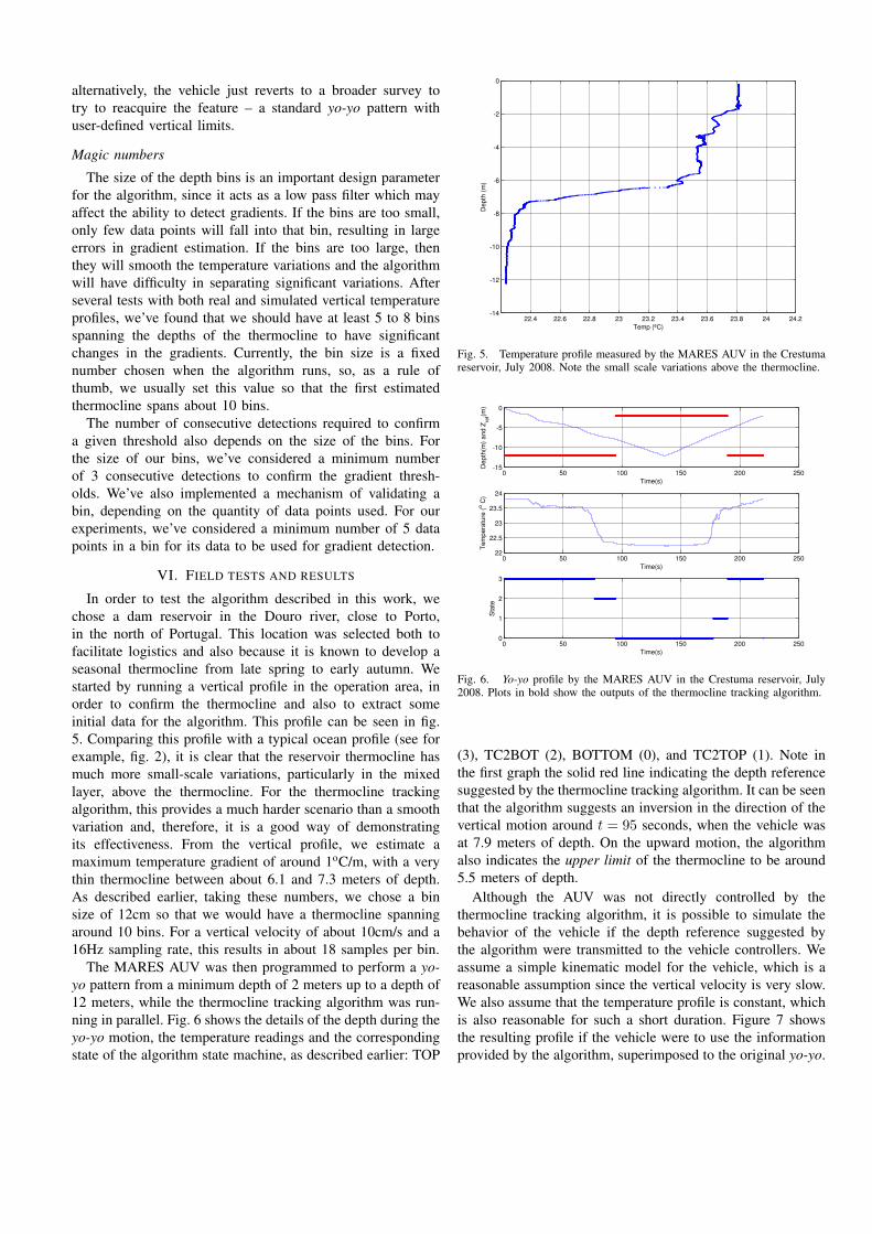
In order to test the algorithm described in this work, wechose a dam reservoir in the Douro river, close to Porto,in the north of Portugal. This location was selected both tofacilitate logistics and also because it is known to develop aseasonal thermocline from late spring to early autumn. Westarted by running a vertical profile in the operation area, inorder to confirm the thermocline and also to extract someinitial data for the algorithm. This profile can be seen in fig.5. Comparing this profile with a typical ocean profile (see forexample, fig. 2), it is clear that the reservoir thermocline hasmuch more small-scale variations, particularly in the mixedlayer, above the thermocline. For the thermocline trackingalgorithm, this provides a much harder scenario than a smoothvariation and, therefore, it is a good way of demonstratingits effectiveness. From the vertical profile, we estimate amaximum temperature gradient of around 1oC/m, with a verythin thermocline between about 6.1 and 7.3 meters of depth.As described earlier, taking these numbers, we chose a binsize of 12cm so that we would have a thermocline spanningaround 10 bins. For a vertical velocity of about 10cm/s and a16Hz sampling rate, this results in about 18 samples per bin.

The MARES AUV was then programmed to perform a yo-yo pattern from a minimum depth of 2 meters up to a depth of12 meters, while the thermocline tracking algorithm was run-ning in parallel. Fig. 6 shows the details of the depth during theyo-yo motion, the temperature readings and the correspondingstate of the algorithm state machine, as described earlier: TOP

Fig. 5. Temperature profile measured by the MARES AUV in the Crestumareservoir, July 2008. Note the small scale variations above the thermocline.

Fig. 6. Yo-yo profile by the MARES AUV in the Crestuma reservoir, July2008. Plots in bold show the outputs of the thermocline tracking algorithm.

(3), TC2BOT (2), BOTTOM (0), and TC2TOP (1). Note inthe first graph the solid red line indicating the depth referencesuggested by the thermocline tracking algorithm. It can be seenthat the algorithm suggests an inversion in the direction of thevertical motion around t = 95 seconds, when the vehicle wasat 7.9 meters of depth. On the upward motion, the algorithmalso indicates the upper limit of the thermocline to be around5.5 meters of depth.

Although the AUV was not directly controlled by thethermocline tracking algorithm, it is possible to simulate thebehavior of the vehicle if the depth reference suggested bythe algorithm were transmitted to the vehicle controllers. Weassume a simple kinematic model for the vehicle, which is areasonable assumption since the vertical velocity is very slow.We also assume that the temperature profile is constant, whichis also reasonable for such a short duration. Figure 7 showsthe resulting profile if the vehicle were to use the informationprovided by the algorithm, superimposed to the original yo-yo.

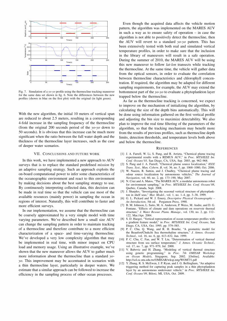
Fig. 7. Simulation of a yo-yo profile using the thermocline tracking maneuverfor the same data set shown in fig. 6. Note the differences between the newprofiles (shown in blue on the first plot) with the original (in light green).

With the new algorithm, the initial 10 meters of vertical spanare reduced to about 2.5 meters, resulting in a corresponding4-fold increase in the sampling frequency of the thermocline(from the original 200 seconds period of the yo-yo down to50 seconds). It is obvious that this increase can be much moresignificant when the ratio between the full water depth and thethickness of the thermocline layer increases, such as the caseof deeper water scenarios.

VII. CONCLUSIONS AND FUTURE WORK

In this work, we have implemented a new approach to AUVsurveys that is to replace the standard predefined mission byan adaptive sampling strategy. Such an approach exploits theon-board computational power to infer some characteristics ofthe oceanographic environment and react to this environmentby making decisions about the best sampling strategy to use.By continuously interpreting collected data, this decision canbe made in real time so that the vehicle can use most of theavailable resources (mainly power) in sampling the ocean inregions of interest. Naturally, this will contribute to faster andmore efficient surveys.

In our implementation, we assume that the thermocline canbe coarsely approximated by a very simple model with timevarying parameters. We’ve described how a small size AUVcan change the sampling pattern in order to maintain trackingof a thermocline and therefore contribute to a more efficientcharacterization of a space- and time-varying thermocline.We’ve developed a very low complexity algorithm that maybe implemented in real time, with minor impact on CPUload and memory usage. Using an illustrative example, we’veshown that the new maneuver allows the AUV to gather muchmore information about the thermocline than a standard yo-yo. This improvement may be accentuated in scenarios witha thin thermocline layer, particularly in deeper waters. Weestimate that a similar approach can be followed to increase theefficiency in the sampling process of other ocean processes.

Even though the acquired data affects the vehicle motionpattern, the algorithm was implemented on the MARES AUVin such a way as to ensure safety of operation – in case thealgorithm is not able to positively detect the thermocline, thenthe AUV will revert to a standard yo-yo pattern. This hasbeen extensively tested with both real and simulated verticaltemperature profiles, in order to make sure that the inclusionin the library of maneuvers will result in a safe operation.During the summer of 2010, the MARES AUV will be usingthis new maneuver to follow lat-lon transects while trackingthe thermocline. At the same time, the vehicle will gather datafrom the optical sensors, in order to evaluate the correlationbetween thermocline characteristics and chlorophyll concen-tration. If required, the algorithm may be adapted for differentsampling requirements, for example, the AUV may extend thebottommost part of the yo-yo to evaluate a phytoplankton layertrapped below the thermocline.

As far as the thermocline tracking is concerned, we expectto improve on the mechanism of initializing the algorithm, bycalculating the size of the depth bins automatically. This willbe done using information gathered on the first vertical profileand adjusting the bin size to maximize detectability. We alsoplan to improve the real time filtering of the parameters of thealgorithm, so that the tracking mechanism may benefit morefrom the results of previous profiles, such as thermocline depthlimits, detection thresholds, and temperature levels both aboveand below the thermocline.

REFERENCES

[1] J. A. Farrell, W. Li, S. Pang, and R. Arrieta, “Chemical plume tracingexperimental results with a REMUS AUV,” in Proc. MTS/IEEE Int.Conf. Oceans’03, San Diego, CA, USA, Sep. 2003, pp. 962–968.

[2] S. Pang and J. A. Farrell, “Chemical plume source localization,” IEEETrans. Syst., Man, Cybern. B, vol. 36, no. 5, pp. 1068–1080, Oct. 2006.

[3] W. Naeem, R. Sutton, and J. Chudley, “Chemical plume tracing andodour source localization by autonomous vehicles,” The Journal ofNavigation, vol. 60, no. 2, pp. 173–190, May 2007.

[4] N. Cruz and A. Matos, “The MARES AUV, a modular autonomous robotfor environment sampling,” in Proc. MTS/IEEE Int. Conf. Oceans’08,Quebec, Canada, Sept. 2008.

[5] J. Sharples, “Investigating the seasonal vertical structure of phytoplank-ton in shelf seas,” Mar. Model., vol. 1, no. 1–4, pp. 3–38, 1999.

[6] G. L. Pickard and W. J. Emery, Descriptive Physical Oceanography –An Introduction, 5th ed. Pergamon Press, 1990.

[7] B. M. Johnson, L. Saito, M. A. Anderson, P. Weiss, M. Andre, and D. G.Fontane, “Effects of climate and dam operations on reservoir thermalstructure,” J. Water Resour. Plann. Manage., vol. 130, no. 2, pp. 112–122, Mar./Apr. 2004.

[8] S. D. Haeger, “Vertical representation of ocean temperature profiles witha gradient feature model,” in Proc. MTS/IEEE Int. Conf. Oceans, SanDiego, CA, USA, Oct. 1995, pp. 579–585.

[9] P. C. Chu, Q. Wang, and R. H. Bourke, “A geometric model forthe Beaufort/Chukchi Sea thermohaline structure,” J. Atmos. OceanicTechnol., vol. 16, no. 6, pp. 613–632, Jun. 1999.

[10] P. C. Chu, C. Fan, and W. T. Liu, “Determination of vertical thermalstructure from sea surface temperature,” J. Atmos. Oceanic Technol.,vol. 17, no. 7, pp. 971–979, Jul. 2000.

[11] V. Babovic and H. Zhang, “Modeling of vertical thermal structureusing genetic programming,” in Proc. 7th OMISAR Workshopon Ocean Models, Singapore, Sep. 2002. [Online]. Available:http://sol.oc.ntu.edu.tw/OMISAR/wksp.mtg/WOM7/1.pdf

[12] Y. Zhang, R. S. McEwen, J. P. Ryan, and J. G. Bellingham, “An adaptivetriggering method for capturing peak samples in a thin phytoplanktonlayer by an autonomous underwater vehicle,” in Proc. MTS/IEEE Int.Conf. Oceans’09, Biloxi, MI, USA, Oct. 2009.