Simulating the Effects of Climate Change on Fraser River Flood Scenarios – Phase 2
Final Report
26 May 2015
Prepared for: Flood Safety Section Ministry of Forests Lands and Natural Resource Operations
Rajesh R. Shrestha
Markus A. Schnorbus
Alex J. Cannon
Francis W. Zwiers
i
Simulating the Effects of Climate Change on Fraser River Flood Scenarios
– Phase 2
EXECUTIVE SUMMARY .................................................................................................................................. ii
1. INTRODUCTION ..................................................................................................................................... 1
1.1 Project Background ........................................................................................................................... 1
1.2 Scope of Work ................................................................................................................................... 2
1.3 Deliverables ....................................................................................................................................... 2
2. METHODS .............................................................................................................................................. 4
2.1 Generalized Extreme Value (GEV) Model ......................................................................................... 4
2.2 Stationary Analysis of Historical Extreme Discharge ........................................................................ 5
2.2.1 Stationary GEV Parameter Estimation .......................................................................................... 6
2.2.2 Plotting Positions .......................................................................................................................... 6
2.3 Nonstationary Analysis of Future Extreme Discharge ...................................................................... 6
2.3.1 Nonstationary GEV Parameter Estimation ................................................................................... 7
2.3.2 Covariates Evaluation ................................................................................................................... 8
2.3.3 Model Implementation and Selection ........................................................................................... 9
3. RESULTS AND DISCUSSION .................................................................................................................. 11
3.1 Stationary Historical Flood Frequency Analysis .............................................................................. 11
3.2 Nonstationary Analysis of Future Extreme Discharge .................................................................... 13
3.2.1 Evaluation of Training and Validation Results ............................................................................ 13
3.2.2 Future Changes in Discharge Quantiles for CMIP3 GCMs ........................................................... 15
3.2.3 Future Changes in Discharge Quantiles for CMIP5 GCMs ........................................................... 21
3.2.4 Uncertainties in Estimating Discharge Quantiles ........................................................................ 25
4. CONCLUSIONS AND FUTURE WORK ................................................................................................... 27
REFERENCES ................................................................................................................................................ 29
LIST OF TABLES ............................................................................................................................................ 33
LIST OF FIGURES .......................................................................................................................................... 34
APPENDIX A: EMISSIONS SCENARIOS ......................................................................................................... 36
APPENDIX B: TABLES ................................................................................................................................... 38
APPENDIX C: FIGURES ................................................................................................................................. 54
ii
EXECUTIVE SUMMARY
Projecting streamflow extremes under nonstationarity is important for managing river flooding in a
changing climate. The objective of this study is to develop a nonstationary modelling framework for
projecting future changes in the annual exceedance probabilities of streamflow extremes for the Fraser
River at Hope station (WSC gauge 08MF005) using phase 5 of the Coupled Model Intercomparison
Project (CMIP5) generation of global climate models (GCMs). Nonstationarity is represented by the
variable parameter Generalized Extreme Value (GEV) distribution, which provides a flexible approach for
estimating the distribution of extremes.
In the first part of this work, a stationary analysis of extreme historical discharge was conducted based
on 102-year (1912-2013) historical annual maximum daily flow data, supplemented with the estimated
1894 peak discharge value. Based on the fitted Gumbel distribution, the 1894 event (≈ 17000 m3/s) has
a return period of about 500 years, with a confidence range (5% to 95%) of 16000 m3/s to 18000 m3/s.
Likewise, an event of 17000 m3/s has a return period that ranges from 250 to 1000 years.
In the second part of this study, a nonstationary flood frequency analysis was conducted with the
parameters of the GEV distribution expressed as a function of climate covariates. The parameters were
estimated using the GEV conditional density network (GEVcdn) with seasonal precipitation and
temperature, which drive the peak streamflow in spring, and time (year) used as covariates. The GEVcdn
model was trained using climate projections and hydrology model output based on the phase 3 of the
Coupled Model Intercomparison Project (CMIP3). The results of the GEVcdn nonstationary model
showed a good ability of the model to simulate quantile discharges. We then projected future flow
quantiles by using covariates taken from latest CMIP5 generation of climate projections. For the
evaluation of the future changes in discharge quantiles, we considered 30-year periods as stationary,
and future change in discharge quantiles were evaluated relative to the historical discharge quantiles
(from the first part of this study).
The future discharge quantiles for the CMIP5-based projections mostly showed increases in flow
magnitudes for the three representative concentration pathways (RCPs)1 and three future periods. In
general, the larger the return period, the larger is the increase in flow magnitude. The median increases
in 2071-2100 based on CMIP5 GCM ensembles are 5% to 15%, 3% to 18% and -3% to 24% (range are for
10 year-10000 year return periods) for RCP 2.6, 4.5 and 8.5, respectively. The maximum increases in
2071-2098 from CMIP5 GCM ensembles are 15% to 53%, 21% to 52% and 22% to 74% for RCP 2.6, 4.5
and 8.5, respectively. The results of this study are affected by a number of different sources of
uncertainties, which arise from the data and model used. In particular, long return periods (e.g. > 1000
year) are affected by uncertainties due to sampling variability, and the results for long return period
events presented in this report should be treated with a caution.
1 Emissions scenarios are summarized in Appendix A
1
1. INTRODUCTION
1.1 Project Background
The Flood Safety Section of the Ministry of Forests, Lands and Natural Resource Operations (FLNRO) and
Northwest Hydraulic Consultants (NHC) completed a joint project on: “Simulating the Effects of Sea
Level Rise and Climate Change on Fraser River Flood Scenarios” (Flood Safety Section, 2014). The
project used the MIKE-11 hydrodynamic model for the Fraser River from Hope to the Strait of Georgia to
generate water surface profiles for peak flow quantiles corresponding to a range of annual exceedance
probabilities (AEPs) derived from historical flow data. Additionally, future water surface profiles for the
same range of AEPs were generated, with the future discharge quantiles derived from the Pacific
Climate Impacts Consortium’s (PCIC’s) projected future hydrologic scenarios (Shrestha et al. 2012) based
on the Variable Infiltration Capacity (VIC) hydrology model simulations. These simulations were based
on climate projections using Global Climate Models (GCMs) and emissions scenarios from phase 3 of the
Coupled Model Intercomparison Project (CMIP3)2.
The purpose of the current study is to update the peak flow quantile projections for the Fraser River at
Hope using climate projections from the more recent phase 5 of the Coupled Model Intercomparison
Project (CMIP5). These peak flow projections will be based on results from a new generation of GCMs
and new emissions scenarios (Appendix A provides a description of the CMIP3 and CMIP5 emissions
scenarios). Given the projected intensification of the global water cycle due to climate change
(Huntington 2006) and natural climate variability, another important consideration for generating future
change in discharge extremes is nonstationarity. This study explicitly considers nonstationarity by using
a variable parameter Generalized Extreme Value (GEV) distribution.
The direct means of estimating peak flow quantiles for given AEPs for CMIP5 would be to force VIC with
the downscaled CMIP5 climate projections. However, CMIP5-based VIC projections are presently (April
2015) unavailable. Given the computational cost and time required for downscaling GCMs and
hydrologic modelling, such a methodology was not considered for this study. As an alternative, a
computationally efficient Generalized Extreme Value conditional density network (GEVcdn) model
(Cannon 2010, 2011), which can estimate nonstationary discharge quantiles based on covariates, was
employed. Climatic covariates derived from an ensemble of 23 CMIP3 projections were used to train
the GEVcdn model to emulate the VIC simulated peak streamflows (Shrestha et al. 2012). The model
was then used to estimate the streamflow peak flow quantiles for the CMIP5 generation of climate
projections. Given that both CMIP3 and CMIP5 projections produced generally warmer and wetter
future climate responses for the Fraser basin (Schnorbus and Cannon 2014), the CMIP3 data was
considered suitable for training the GEVcdn model. Similar methodology - statistical emulation of the
monthly streamflow projections for the CMIP3 GCMs and simulation of for CMIP5 GCMs - was used by
Schnorbus and Cannon (2014).
2More information on the Coupled Model Intercomparison Project can be found at http://cmip-
pcmdi.llnl.gov/index.html?submenuheader=0 (last accessed April 30, 2015)
2
1.2 Scope of Work
1.2.1. Setup of a stationary statistical model for the historical streamflow extremes data.
The GEV distribution was fit to the historical data (1912-2013) augmented with historical peak
discharge values composed of a single extreme flood magnitude.
1.2.2. Setup of a nonstationary statistical model for approximating the relationship between
climate variables (i.e., precipitation and temperature) and streamflow extremes. After
reviewing previous studies on statistical modelling of climate extremes (e.g., Kharin and Zwiers
2005; Cannon 2010; Zhang et al. 2010; Kharin et al. 2013; Vasiliades et al. 2014) and streamflow
extremes (e.g., Towler et al. 2010; Salas and Obeysekera 2014; Condon et al. 2015), the GEVcdn
nonstationary model was setup for linking the CMIP3 precipitation and temperature covariates
with the VIC model simulated streamflow extremes for the Fraser River at Hope station that are
extracted from VIC simulations driven with the same CMIP3 GCMs.
1.2.3. Evaluation of the performance of the nonstationary statistical model. A number of
combinations of covariates were considered for modelling the streamflow extremes. After
evaluating the performance of the different covariate combinations, the model with the best
statistical performance was chosen.
1.2.4. Projection of future flow quantiles using statistical model. Using the nonstationary
GEV statistical mode, peak flow quantiles were resampled from the 30-year baseline (1961-
1990), and 30-year (2011-2040 and 2041-2070) and 28-year (2071-2098) future periods. GEV
distributions were next fit to the resampled data assuming stationarity within each 30-year
period. The baseline and future flood frequency distributions were then used to estimate the
percentage change in future discharge quantiles for given AEPs. The percentage change values
were then used to scale the historical discharge quantiles (section 1.2.1), thus obtaining
estimates of projected future discharge quantiles.
1.3 Deliverables
Based on the project proposal, PCIC prepared this report by including the following deliverables:
Annual maximum discharge data and plotting positions for the historical stationary flood
frequency analysis.
Model calibration and validation results for the nonstationary flood frequency analysis.
Future flood frequency curves for the CMIP3 and CMIP5 GCMs for return periods extending
from 10 to 10,000 years.
3
A table showing percent change in projected discharges for 10-year, 50-year, 100-year, 200-year,
500-year, 1000-year, 2000-year, 5000-year, and 10000-year return periods (for Timespan1=
2011 to 2040, Timespan2= 2041 to 2070, and Timespan3= 2071 to 2098).
A table with projected discharges for 10-year, 50-year, 100-year, 200-year, 500-year, 1000-year,
2000-year, 5000-year, and 10000-year return periods.
Boxplots showing statistical distribution of discharges from multiple GCMs, emissions scenarios,
and future periods.
4
2. METHODS
2.1 Generalized Extreme Value (GEV) Model
Extreme value theory provides a basis for modelling the maxima or minima of a data series. On the
basis of an underlying asymptotic argument, the theory allows for extrapolation beyond observed
events (Coles 2001; Towler et al. 2010) using the generalized extreme value (GEV) distribution. The
cumulative distribution function (CDF) of the GEV can be expressed as:
𝐹(𝑥, 𝜃) = exp [− {1 + 𝜉 (𝑥 − 𝜇
𝜎)}
−1/𝜉
]
for 𝜉 ≠ 0, 1 + 𝜉 (𝑥−𝜇
𝜎) > 0
(1)
𝐹(𝑥, 𝜃) = exp [−exp {− (𝑥 − 𝜇
𝜎)}]
for 𝜉 = 0
(2)
where 𝜃 = (𝜇, 𝜎, 𝜉) are the location (𝜇), scale (𝜎 > 0) and shape (𝜉) parameters of the GEV distribution
and x denotes the annual streamflow maximum value (in this case). The location and scale parameters
represent the centre and spread of the distribution, respectively. Based on the shape parameter, which
characterizes the distribution’s tail, the GEV can assume three types: (I) 𝜉 = 0 light-tailed or Gumbel
type. (II) 𝜉 > 0 heavy-tailed or Fréchet type; and (III) 𝜉 < 0 bounded tail or Weibull type. Note that the
parameterization of equations (1) and (2) follows the convention in Towler et al. (2010) – in the hydro-
climatological literature it is also common to parameterize 𝜉∗ = −𝜉 (e.g., Kharin and Zwiers 2005;
Cannon 2010).
From equations (1) and (2), the probabilistic quantile 𝑥𝜏 can be obtained:
𝑥𝜏 = 𝜇 −𝜎
𝜉[1 − {−log(𝜏)}−𝜉], 𝜉 ≠ 0 (3)
𝑥𝜏 = 𝜇 − 𝜎𝑙𝑜𝑔{−𝑙𝑜𝑔(𝜏)}, 𝜉 = 0
(4)
where 𝜏 is the non-exceedance probability with the exceedance probability 𝑝 = (1 − 𝜏) and 0 < 𝜏 < 1 ,
and the annual maxima (or minima) 𝑥𝜏 corresponds to the return period 𝑇 = 1/(1 − 𝜏).
The distribution can represent either stationary or nonstationary conditions by using either constant or
variables (one or more) GEV parameters, respectively. Nonstationary parameters can be described as
functions of covariates. Under stationarity, a T-year event has two equivalent interpretations. The first
interpretation is that the expected waiting time for an event until the next exceedance is T-years. The
second interpretation is that the size of an event 𝑥𝜏 has probability 1/T of exceedence in any given year
(Wilks 2006; Cooley 2013). In contrast, in the non-stationary case the return value becomes covariate
dependent, and thus only the latter (instantaneous risk) interpretation is possible.
5
2.2 Stationary Analysis of Historical Extreme Discharge
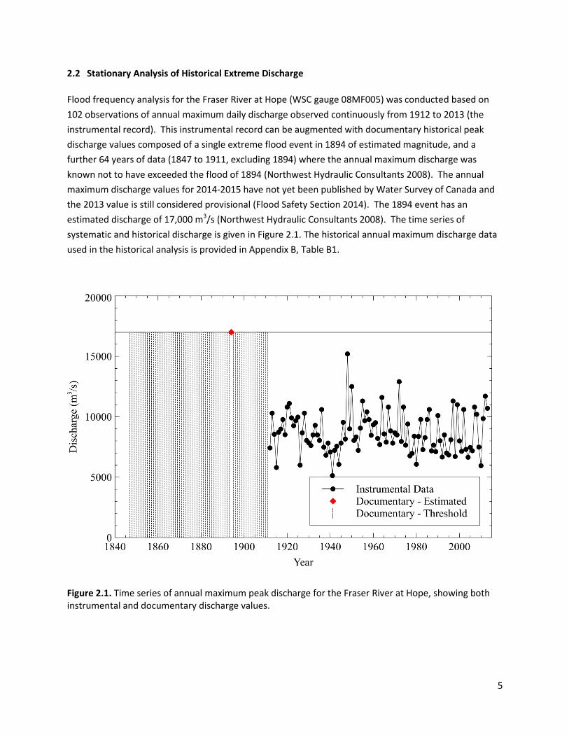
Flood frequency analysis for the Fraser River at Hope (WSC gauge 08MF005) was conducted based on
102 observations of annual maximum daily discharge observed continuously from 1912 to 2013 (the
instrumental record). This instrumental record can be augmented with documentary historical peak
discharge values composed of a single extreme flood event in 1894 of estimated magnitude, and a
further 64 years of data (1847 to 1911, excluding 1894) where the annual maximum discharge was
known not to have exceeded the flood of 1894 (Northwest Hydraulic Consultants 2008). The annual
maximum discharge values for 2014-2015 have not yet been published by Water Survey of Canada and
the 2013 value is still considered provisional (Flood Safety Section 2014). The 1894 event has an
estimated discharge of 17,000 m3/s (Northwest Hydraulic Consultants 2008). The time series of
systematic and historical discharge is given in Figure 2.1. The historical annual maximum discharge data
used in the historical analysis is provided in Appendix B, Table B1.
Figure 2.1. Time series of annual maximum peak discharge for the Fraser River at Hope, showing both instrumental and documentary discharge values.
6
2.2.1 Stationary GEV Parameter Estimation
Initial parameter estimation made use of the complete set of instrumental and documentary data in
order to maintain consistency with previous work (Northwest Hydraulic Consultants 2008). For this
initial approach we used Maximum likelihood (ML) estimation, an efficient and flexible approach which
can easily incorporate all manner of historic information (Stedinger et al. 1993; Payrastre et al. 2011).
We explored GEV parameter estimation using three different target data sets:
1) combined instrumental and documentary data (n=167);
2) only instrumental data (n=102); and
3) instrumental data, but including the 1894 event as an additional observation (n=103).
2.2.2 Plotting Positions
Probability plotting positions are used for the graphical display of flood peaks and as an empirical
estimate of the probability of exceedance. In order to estimate the exceedance probability of annual
maximum flood discharges comprised of both instrumental records as well as documentary records, we
use the plotting positions suggested by Hirsch and Stedinger (1987). Following the nomenclature of
Hirsch and Stedinger (1987), let n be the length (in years) of the historical period over which a set of
flood events can be ranked, let s be the length of the systematic record period and let g consist of the
complete record of observed floods where n>g>s. Among these floods there is a subset of
“extraordinary” floods which are known to have ranks 1 through k over the period of length n, and let e
be the number of extraordinary floods from the 1912-2013 record, where e ≤ k and g = s + k – e. Plotting
positions have been calculated as:
�̂�𝑖 = {𝑝𝑒
𝑖 − 𝛼
𝑘 + 1 − 2𝛼𝑖 = 1, … , 𝑘
𝑝𝑒 + (1 − 𝑝𝑒)𝑖 − 𝑘 − 𝑎
𝑠 − 𝑒 + 1 − 2𝑎𝑖 = 𝑘 + 1,… , 𝑔
(5)
where �̂�𝑖 is the estimated exceedance probability, 𝑝𝑒 is the probability of exceedance above the
threshold yT, estimated as k/n.
2.3 Nonstationary Analysis of Future Extreme Discharge
Presently (March 2015), streamflow projections based on the CMIP5 GCMs are unavailable. Given the
computational cost and time required for downscaling GCMs and hydrologic modelling, a
computationally efficient Generalized Extreme Value conditional density network (GEVcdn) model
proposed by Cannon (2010, 2011) was employed. The model was developed and trained with inputs
derived from the CMIP3 generation of GCMs and targets obtained from the corresponding VIC simulated
7
peak streamflows (Shrestha et al. 2012). The model was then used to derive the discharge quantiles for
the CMIP5 generation of the GCMs.
2.3.1 Nonstationary GEV Parameter Estimation
The “GEVcdn” R package (Cannon 2014) was employed for the evaluation of the GEV parameters. The
GEVcdn is a probabilistic extension of the multilayer perceptron neural network, which expresses the
GEV parameters as nonlinear function of covariates. Due to its nonlinear architecture, the model is
capable of representing a wide range of nonstationary relationships, including interactions between
covariates.
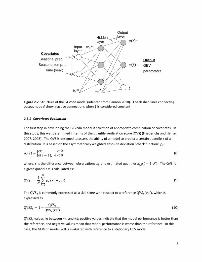
The GEVcdn structure consists of a three-layer interconnected network model (Cannon 2010), with the
first (input) layer providing connections to the covariates, the second (hidden) layer providing
connections to all inputs in the first layer, and the third (output) layer providing outputs in the form GEV
parameters (Figure 2.2). Given covariates at time t, 𝑥(𝑡) = {𝑥𝑖(𝑡), 𝑖 = 1: 𝐼}, the output from the jth
hidden layer node h𝑗(𝑡) is given by transforming the signals using an activation function 𝑓(. ):
h𝑗(𝑡) = 𝑓 (∑𝑤𝑗𝑖(𝑛)𝑥𝑖(𝑡) + 𝑏𝑗
(𝑛)
𝐼
𝑖=1
) (6)
Where, 𝑤𝑗𝑖(𝑛) is a hidden layer weight and 𝑏𝑗
(𝑛)is a bias at node 𝑛 = 1:𝑁. The activation function 𝑓(. )
is taken to be the sigmoidal function 1/(1 + 𝑒−(.)) or hyperbolic tangent function tanh(. ) for the
nonlinear GEVcdn network and identity function for the strictly linear GEVcdn network. Similarly, the
value at an output layer node 𝑂𝑘(𝑡) (𝑚 = 1: 3) is obtained as:
𝑂𝑘(𝑡) = 𝑓 (∑𝑤𝑘𝑗(𝑚)ℎ𝑗(𝑡) + 𝑏𝑘
(𝑚)
𝐽
𝑗=1
) (7)
The output layer activation functions depend on the GEV parameter: identity for 𝜇, exp(. ) for 𝜎 (to
ensure positivity), and 0.5 ∗ tanh(. ) for 𝜉 (to ensure values between -0.5 to 0.5):
The GEVcdn model parameters were estimated by using the ML approach (described in section 2.2.1)
with the quasi-Newton algorithm used for optimization. The appropriate GEVcdn model hyper-
parameters (i.e., number of hidden nodes and activation function) for a given dataset was selected by
fitting models with different hyper-parameters and choosing the one that minimizes the Akaike
information criterion with small sample size correction (AICc) (Akaike 1974; Hurvich and Tsai 1989). The
AICc chooses the most parsimonious model that is capable of accounting for the true (but unknown)
deterministic function responsible for generating the observations, thus, avoiding overfitting (fits the
data to the noise rather than underlying signal) (Cannon 2010). Additionally, a part of the available data
was kept aside (spilt-sampling) for an independent validation of the results.
8
Figure 2.2. Structure of the GEVcdn model (adapted from Cannon 2010). The dashed lines connecting output node 𝝃 show inactive connections when 𝝃 is considered constant.
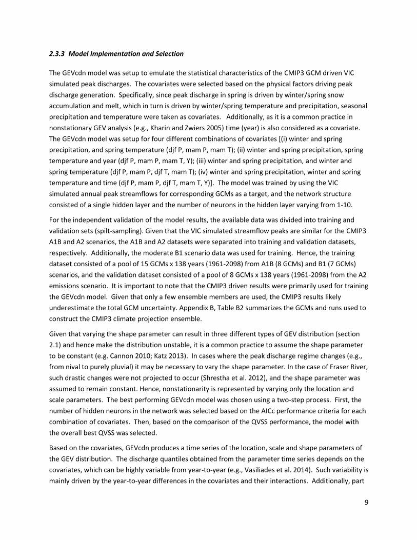
2.3.2 Covariates Evaluation
The first step in developing the GEVcdn model is selection of appropriate combination of covariates. In
this study, this was determined in terms of the quantile verification score (QVS) (Friederichs and Hense
2007, 2008). The QVS is designed to assess the ability of a model to predict a certain quantile 𝜏 of a
distribution. It is based on the asymmetrically weighted absolute deviation “check function” 𝜌𝜏:
𝜌𝜏(𝜖) = {𝜖𝜏, ≥ 0𝜖(𝜏 − 1),𝜖 < 0
(8)
where, 𝜖 is the difference between observations 𝑥𝑖and estimated quantiles 𝑧𝜏,𝑖(𝑖 = 1:𝑁). The QVS for
a given quantile 𝜏 is calculated as:
QVS𝜏 =1
𝑁∑𝜌𝜏(𝑥𝑖 − 𝑧𝜏,𝑖)
𝑁
𝑖=1
(9)
The QVS𝜏 is commonly expressed as a skill score with respect to a reference QVS𝜏(ref), which is
expressed as.
QVSS𝜏 = 1 −QVS𝜏
QVS𝜏(ref) (10)
QVSS𝜏 values lie between −∞ and +1; positive values indicate that the model performance is better than
the reference, and negative values mean that model performance is worse than the reference. In this
case, the GEVcdn model skill is evaluated with reference to a stationary GEV model.
)
(m) (n)
(t)
(t)
(m)
(n) Input layer
Hidden layer
Covariates
Seasonal prec.
Seasonal temp.
Time (year)
Output
GEV
parameters
Output layer
9
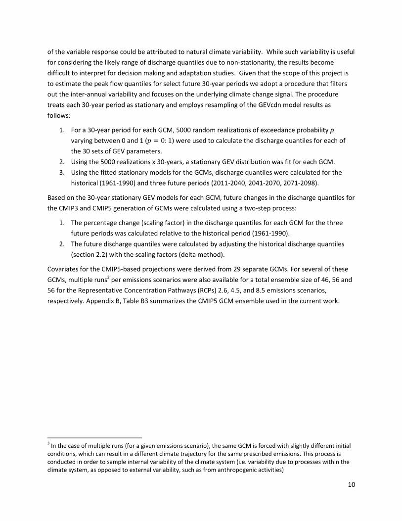
2.3.3 Model Implementation and Selection
The GEVcdn model was setup to emulate the statistical characteristics of the CMIP3 GCM driven VIC
simulated peak discharges. The covariates were selected based on the physical factors driving peak
discharge generation. Specifically, since peak discharge in spring is driven by winter/spring snow
accumulation and melt, which in turn is driven by winter/spring temperature and precipitation, seasonal
precipitation and temperature were taken as covariates. Additionally, as it is a common practice in
nonstationary GEV analysis (e.g., Kharin and Zwiers 2005) time (year) is also considered as a covariate.
The GEVcdn model was setup for four different combinations of covariates [(i) winter and spring
precipitation, and spring temperature (djf P, mam P, mam T); (ii) winter and spring precipitation, spring
temperature and year (djf P, mam P, mam T, Y); (iii) winter and spring precipitation, and winter and
spring temperature (djf P, mam P, djf T, mam T); (iv) winter and spring precipitation, winter and spring
temperature and time (djf P, mam P, djf T, mam T, Y)]. The model was trained by using the VIC
simulated annual peak streamflows for corresponding GCMs as a target, and the network structure
consisted of a single hidden layer and the number of neurons in the hidden layer varying from 1-10.
For the independent validation of the model results, the available data was divided into training and
validation sets (spilt-sampling). Given that the VIC simulated streamflow peaks are similar for the CMIP3
A1B and A2 scenarios, the A1B and A2 datasets were separated into training and validation datasets,
respectively. Additionally, the moderate B1 scenario data was used for training. Hence, the training
dataset consisted of a pool of 15 GCMs x 138 years (1961-2098) from A1B (8 GCMs) and B1 (7 GCMs)
scenarios, and the validation dataset consisted of a pool of 8 GCMs x 138 years (1961-2098) from the A2
emissions scenario. It is important to note that the CMIP3 driven results were primarily used for training
the GEVcdn model. Given that only a few ensemble members are used, the CMIP3 results likely
underestimate the total GCM uncertainty. Appendix B, Table B2 summarizes the GCMs and runs used to
construct the CMIP3 climate projection ensemble.
Given that varying the shape parameter can result in three different types of GEV distribution (section
2.1) and hence make the distribution unstable, it is a common practice to assume the shape parameter
to be constant (e.g. Cannon 2010; Katz 2013). In cases where the peak discharge regime changes (e.g.,
from nival to purely pluvial) it may be necessary to vary the shape parameter. In the case of Fraser River,
such drastic changes were not projected to occur (Shrestha et al. 2012), and the shape parameter was
assumed to remain constant. Hence, nonstationarity is represented by varying only the location and
scale parameters. The best performing GEVcdn model was chosen using a two-step process. First, the
number of hidden neurons in the network was selected based on the AICc performance criteria for each
combination of covariates. Then, based on the comparison of the QVSS performance, the model with
the overall best QVSS was selected.
Based on the covariates, GEVcdn produces a time series of the location, scale and shape parameters of
the GEV distribution. The discharge quantiles obtained from the parameter time series depends on the
covariates, which can be highly variable from year-to-year (e.g., Vasiliades et al. 2014). Such variability is
mainly driven by the year-to-year differences in the covariates and their interactions. Additionally, part
10
of the variable response could be attributed to natural climate variability. While such variability is useful
for considering the likely range of discharge quantiles due to non-stationarity, the results become
difficult to interpret for decision making and adaptation studies. Given that the scope of this project is
to estimate the peak flow quantiles for select future 30-year periods we adopt a procedure that filters
out the inter-annual variability and focuses on the underlying climate change signal. The procedure
treats each 30-year period as stationary and employs resampling of the GEVcdn model results as
follows:
1. For a 30-year period for each GCM, 5000 random realizations of exceedance probability p
varying between 0 and 1 (𝑝 = 0: 1) were used to calculate the discharge quantiles for each of
the 30 sets of GEV parameters.
2. Using the 5000 realizations x 30-years, a stationary GEV distribution was fit for each GCM.
3. Using the fitted stationary models for the GCMs, discharge quantiles were calculated for the
historical (1961-1990) and three future periods (2011-2040, 2041-2070, 2071-2098).
Based on the 30-year stationary GEV models for each GCM, future changes in the discharge quantiles for
the CMIP3 and CMIP5 generation of GCMs were calculated using a two-step process:
1. The percentage change (scaling factor) in the discharge quantiles for each GCM for the three
future periods was calculated relative to the historical period (1961-1990).
2. The future discharge quantiles were calculated by adjusting the historical discharge quantiles
(section 2.2) with the scaling factors (delta method).
Covariates for the CMIP5-based projections were derived from 29 separate GCMs. For several of these
GCMs, multiple runs3 per emissions scenarios were also available for a total ensemble size of 46, 56 and
56 for the Representative Concentration Pathways (RCPs) 2.6, 4.5, and 8.5 emissions scenarios,
respectively. Appendix B, Table B3 summarizes the CMIP5 GCM ensemble used in the current work.
3 In the case of multiple runs (for a given emissions scenario), the same GCM is forced with slightly different initial
conditions, which can result in a different climate trajectory for the same prescribed emissions. This process is conducted in order to sample internal variability of the climate system (i.e. variability due to processes within the climate system, as opposed to external variability, such as from anthropogenic activities)

11
3. RESULTS AND DISCUSSION
3.1 Stationary Historical Flood Frequency Analysis
Estimated quantile values were found to have little difference (not shown) based on parameters
estimated using the three different data sets: 1) combined instrumental and documentary data (n=167);
2) only instrumental data (n=102); instrumental data, but treating the 1894 event as an additional
observation (n=103). It is apparent that given the relatively long instrumental record for this site, the
addition of documentary data has little overall effect on the quantile estimates. Fitting of the GEV
distribution also reveals that the shape parameter is close to zero (|ξ| < 0.01), indicating that the GEV
Type I distribution (Gumbel) is appropriate for modelling historical peak flow frequency. Further, as
documentary data is not required, parameters can be estimated using the simpler method of L-
moments (e.g. Stedinger et al. 1993), which provides very similar results to ML estimates. Hence, the
historical peak flow frequency for the Fraser River at Hope is estimated by fitting the GEV Type I
(Gumbel) distribution to the instrumental record augmented with the 1894 event (n=103) using the
method of L-moments. The L-moment Gumbel estimates for the Fraser River at Hope are given in Table
3.1 and the empirical quantiles and the fitted Gumbel distribution is shown in Figures 3.1 and 3.2.
Quantile estimates are also summarized in Table 3.2.
Approximate confidence intervals for both distribution parameters and quantiles are estimated by
assuming that both parameters and quantiles are asymptotically normally distributed (Stedinger et al.
1993). The variance of the GEV Type I parameters and quantile variances are calculated from formulas
provided by Phien (1987). Quantile uncertainty can be large, particularly at the higher return periods.
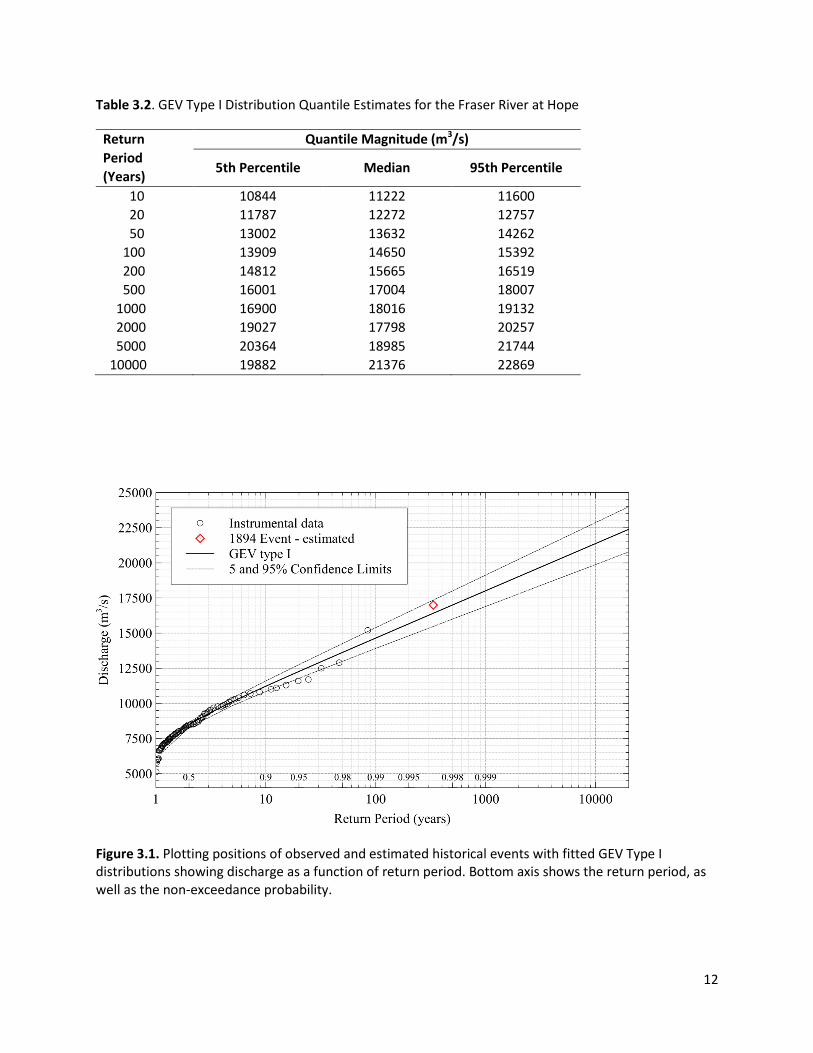
For instance, the 1894 event has an estimated return period ~500 years (Figure 3.1 and Table 3.2), but
the magnitude of a 500-year event has 5 to 95% confidence range of 16000 m3/s to 18000 m3/s (Figure
3.1). Likewise, the return period for an event of 17000 m3/s magnitude ranges from 250 years to 1000
years (based on 5% to 95% confidence limits; Figure 3.2).
It is to be noted that the estimated long return period (1000-10000 years) quantile values are affected
by a number of uncertainties, such as due to a limited number of sample points and changes in river
geomorphological and watershed characteristics. Therefore, the long return period values presented in
this and other sections of this report should be treated with a caution.
Table 3.1. L-moment Gumbel parameter estimates
Parameter Parameter values
5th Percentile Median 95th Percentile
µ 7744 7939 8134
σ 1293 1459 1625
12
Table 3.2. GEV Type I Distribution Quantile Estimates for the Fraser River at Hope
Return
Period
(Years)
Quantile Magnitude (m3/s)
5th Percentile Median 95th Percentile
10 10844 11222 11600
20 11787 12272 12757
50 13002 13632 14262
100 13909 14650 15392
200 14812 15665 16519
500 16001 17004 18007
1000 16900 18016 19132
2000 19027 17798 20257
5000 20364 18985 21744
10000 19882 21376 22869
Figure 3.1. Plotting positions of observed and estimated historical events with fitted GEV Type I distributions showing discharge as a function of return period. Bottom axis shows the return period, as well as the non-exceedance probability.

13
Figure 3.2. Plotting positions of observed and estimated historical events with fitted GEV Type I distributions showing return period as a function of discharge. Left axis shows the return period, as well as the non-exceedance probability.
3.2 Nonstationary Analysis of Future Extreme Discharge
3.2.1 Evaluation of Training and Validation Results
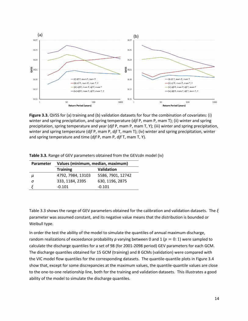
The Quantile Verification Skill Score (QVSS) for the training dataset using the four different combinations
of covariates are shown in Figure 3.3a. In all cases, the stationary model was used as a reference.
Relative to the reference model, all four nonstationary models showed positive skills ranging between
0.17 and 0.26. Comparing the results with and without time as a covariate, i.e., (i) vs. (ii), and (iii) vs. (iv),
in both cases, the results show better QVSS scores when time is used as a covariate. Overall, the results
for the training dataset showed a superior model performance for the model trained with winter and
spring precipitation, winter and spring temperature and time (djf P, mam P, djf T, mam T, Y), except for
1000-year return period. Based on the results, model (iv) was selected as the best model for the
evaluation of the CMIP3 and CMIP5 quantile discharges. Similar results were also obtained for the
validation dataset (Figure 3.3b), with the stationary GEV parameters obtained from the training dataset
used as the reference model.
14
Figure 3.3. QVSS for (a) training and (b) validation datasets for four the combination of covariates: (i) winter and spring precipitation, and spring temperature (djf P, mam P, mam T); (ii) winter and spring precipitation, spring temperature and year (djf P, mam P, mam T, Y); (iii) winter and spring precipitation, winter and spring temperature (djf P, mam P, djf T, mam T); (iv) winter and spring precipitation, winter and spring temperature and time (djf P, mam P, djf T, mam T, Y).
Table 3.3. Range of GEV parameters obtained from the GEVcdn model (iv)
Parameter Values (minimum, median, maximum)
Training Validation
µ 4792, 7984, 13103 5586, 7901, 12742
σ 333, 1184, 2395 630, 1196, 2875
ξ -0.101 -0.101
Table 3.3 shows the range of GEV parameters obtained for the calibration and validation datasets. The ξ
parameter was assumed constant, and its negative value means that the distribution is bounded or
Weibull type.
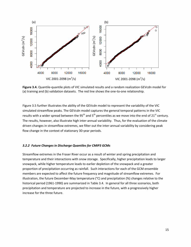
In order the test the ability of the model to simulate the quantiles of annual maximum discharge,
random realizations of exceedance probability p varying between 0 and 1 (𝑝 = 0: 1) were sampled to
calculate the discharge quantiles for a set of 98 (for 2001-2098 period) GEV parameters for each GCM.
The discharge quantiles obtained for 15 GCM (training) and 8 GCMs (validation) were compared with
the VIC model flow quantiles for the corresponding datasets. The quantile-quantile plots in Figure 3.4
show that, except for some discrepancies at the maximum values, the quantile-quantile values are close
to the one-to-one relationship line, both for the training and validation datasets. This illustrates a good
ability of the model to simulate the discharge quantiles.
(a) (b)
15
Figure 3.4. Quantile-quantile plots of VIC simulated results and a random realization GEVcdn model for (a) training and (b) validation datasets. The red line shows the one-to-one relationship.
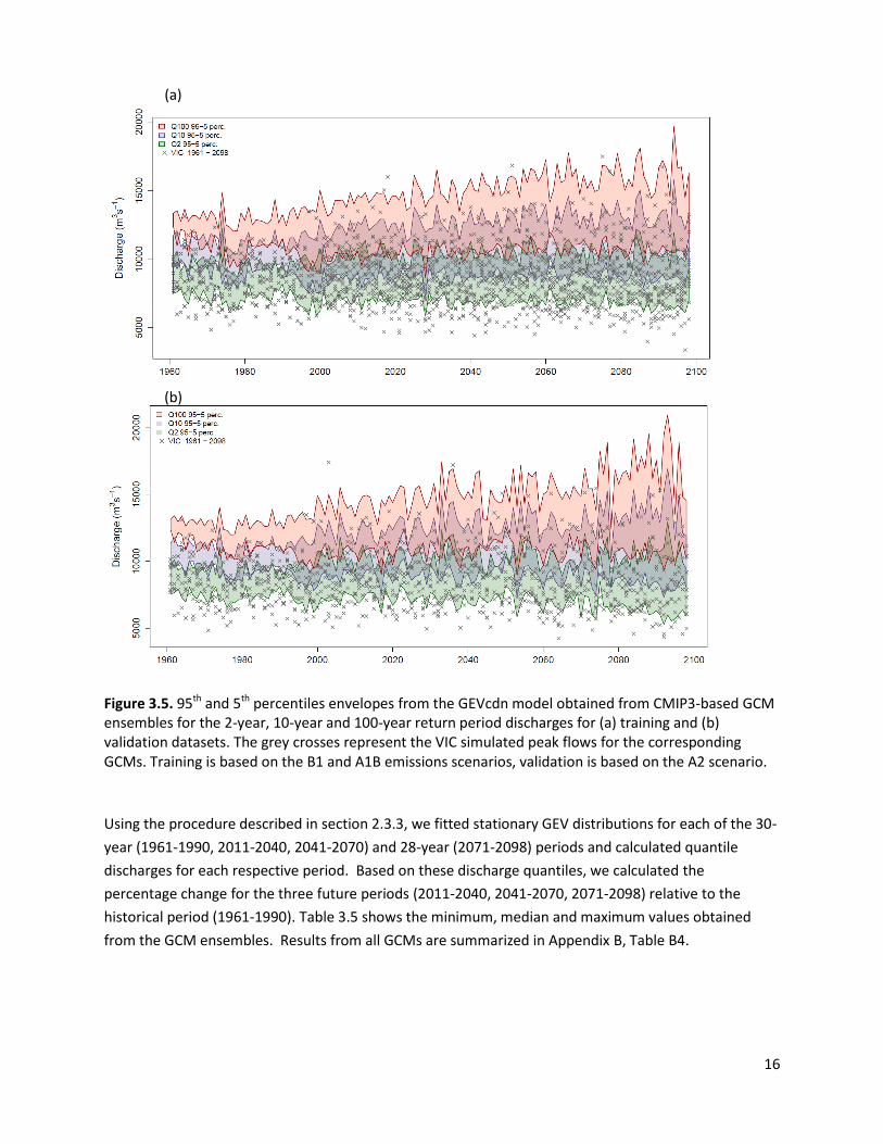
Figure 3.5 further illustrates the ability of the GEVcdn model to represent the variability of the VIC
simulated streamflow peaks. The GEVcdn model captures the general temporal patterns in the VIC
results with a wider spread between the 95th and 5th percentiles as we move into the end of 21st century.
The results, however, also illustrate high inter-annual variability. Thus, for the evaluation of the climate
driven changes in streamflow extremes, we filter out the inter-annual variability by considering peak
flow change in the context of stationary 30-year periods.
3.2.2 Future Changes in Discharge Quantiles for CMIP3 GCMs
Streamflow extremes in the Fraser River occur as a result of winter and spring precipitation and
temperature and their interactions with snow storage. Specifically, higher precipitation leads to larger
snowpack, while higher temperature leads to earlier depletion of the snowpack and a greater
proportion of precipitation occurring as rainfall. Such interactions for each of the GCM ensemble
members are expected to affect the future frequency and magnitude of streamflow extremes. For
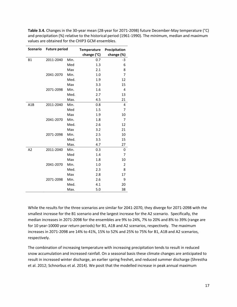
illustration, the future December-May temperature (°C) and precipitation (%) changes relative to the
historical period (1961-1990) are summarized in Table 3.4. In general for all three scenarios, both
precipitation and temperature are projected to increase in the future, with a progressively higher
increase for the three future.
VIC 2001-2098 (m3/s)
GEV
cdn
(m
3/s
)
(a) (b)
VIC 2001-2098 (m3/s)
GEV
cdn
(m
3 /s)
16
Figure 3.5. 95th and 5th percentiles envelopes from the GEVcdn model obtained from CMIP3-based GCM ensembles for the 2-year, 10-year and 100-year return period discharges for (a) training and (b) validation datasets. The grey crosses represent the VIC simulated peak flows for the corresponding GCMs. Training is based on the B1 and A1B emissions scenarios, validation is based on the A2 scenario.
Using the procedure described in section 2.3.3, we fitted stationary GEV distributions for each of the 30-
year (1961-1990, 2011-2040, 2041-2070) and 28-year (2071-2098) periods and calculated quantile
discharges for each respective period. Based on these discharge quantiles, we calculated the
percentage change for the three future periods (2011-2040, 2041-2070, 2071-2098) relative to the
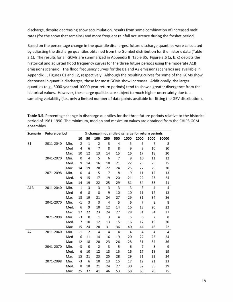
historical period (1961-1990). Table 3.5 shows the minimum, median and maximum values obtained
from the GCM ensembles. Results from all GCMs are summarized in Appendix B, Table B4.
(a)
(b)
17
Table 3.4. Changes in the 30-year mean (28-year for 2071-2098) future December-May temperature (°C) and precipitation (%) relative to the historical period (1961-1990). The minimum, median and maximum values are obtained for the CHIP3 GCM ensembles.
Scenario Future period Temperature
change (°C)
Precipitation
change (%)
B1 2011-2040 Min. 0.7 -3
Med 1.3 6
Max 2.1 8
2041-2070 Min. 1.0 7
Med. 1.9 12
Max 3.3 15
2071-2098 Min. 1.6 4
Med. 2.7 13
Max. 4.5 21
A1B 2011-2040 Min. 0.8 4
Med 1.5 7
Max 1.9 10
2041-2070 Min. 1.8 7
Med. 2.6 12
Max 3.2 21
2071-2098 Min. 2.5 10
Med. 3.5 15
Max. 4.7 27
A2 2011-2040 Min. 0.3 0
Med 1.4 7
Max 1.8 10
2041-2070 Min. 1.0 2
Med. 2.3 8
Max 2.8 17
2071-2098 Min. 2.6 9
Med. 4.1 20
Max. 5.0 38
While the results for the three scenarios are similar for 2041-2070, they diverge for 2071-2098 with the
smallest increase for the B1 scenario and the largest increase for the A2 scenario. Specifically, the
median increases in 2071-2098 for the ensembles are 9% to 24%, 7% to 20% and 8% to 39% (range are
for 10 year-10000 year return periods) for B1, A1B and A2 scenarios, respectively. The maximum
increases in 2071-2098 are 14% to 41%, 15% to 52% and 25% to 75% for B1, A1B and A2 scenarios,
respectively.
The combination of increasing temperature with increasing precipitation tends to result in reduced
snow accumulation and increased rainfall. On a seasonal basis these climate changes are anticipated to
result in increased winter discharge, an earlier spring freshet, and reduced summer discharge (Shrestha
et al. 2012; Schnorbus et al. 2014). We posit that the modelled increase in peak annual maximum
18
discharge, despite decreasing snow accumulation, results from some combination of increased melt
rates (for the snow that remains) and more frequent rainfall occurrence during the freshet period.
Based on the percentage change in the quantile discharges, future discharge quantiles were calculated
by adjusting the discharge quantiles obtained from the Gumbel distribution for the historic data (Table
3.1). The results for all GCMs are summarized in Appendix B, Table B5. Figure 3.6 (a, b, c) depicts the
historical and adjusted flood frequency curves for the three future periods using the moderate A1B
emissions scenario. The flood frequency curves for the B1 and A2 emissions scenarios are available in
Appendix C, Figures C1 and C2, respectively. Although the resulting curves for some of the GCMs show
decreases in quantile discharges, those for most GCMs show increases. Additionally, the larger
quantiles (e.g., 5000-year and 10000-year return periods) tend to show a greater divergence from the
historical values. However, these large qualities are subject to much higher uncertainty due to a
sampling variability (i.e., only a limited number of data points available for fitting the GEV distribution).
Table 3.5. Percentage change in discharge quantiles for the three future periods relative to the historical period of 1961-1990. The minimum, median and maximum values are obtained from the CHIP3 GCM ensembles.
Scenario Future period % change in quantile discharge for return periods
10 50 100 200 500 1000 2000 5000 10000
B1 2011-2040 Min. -2 1 2 3 4 5 6 7 8
Med 4 6 7 8 8 9 9 10 10
Max 10 12 13 14 15 16 17 18 20
2041-2070 Min. 0 4 5 6 7 9 10 11 12
Med. 9 14 16 18 21 22 23 25 25
Max 14 19 20 22 24 25 27 29 30
2071-2098 Min. 0 4 5 7 8 9 11 12 13
Med. 9 15 17 19 20 21 22 23 24
Max. 14 19 22 25 29 31 34 38 41
A1B 2011-2040 Min. 1 3 3 3 3 3 3 4 4
Med 6 8 8 9 10 10 11 12 13
Max 13 19 21 24 27 29 31 34 36
2041-2070 Min. -1 3 3 4 5 6 7 8 8
Med. 6 9 10 12 14 16 18 20 22
Max 17 22 23 24 27 28 31 34 37
2071-2098 Min. -3 0 1 3 4 5 6 7 8
Med. 7 10 12 13 15 16 17 19 20
Max. 15 24 28 31 36 40 44 48 52
A2 2011-2040 Min. -1 2 4 4 4 4 4 4 4
Med 6 11 14 16 19 20 22 23 24
Max 12 18 20 23 26 28 31 34 36
2041-2070 Min. -3 0 2 3 5 6 7 8 9
Med. 6 10 12 13 15 16 17 18 19
Max 15 21 23 25 28 29 31 33 34
2071-2098 Min. -3 6 10 13 15 17 19 21 23
Med. 8 18 21 24 27 30 32 35 39
Max. 25 37 41 46 53 58 63 70 75
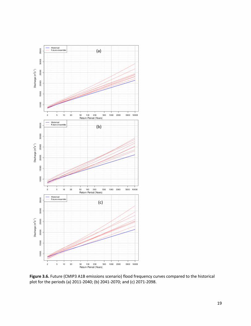
19
Figure 3.6. Future (CMIP3 A1B emissions scenario) flood frequency curves compared to the historical plot for the periods (a) 2011-2040; (b) 2041-2070; and (c) 2071-2098.
(a)
(b)
(c)
20
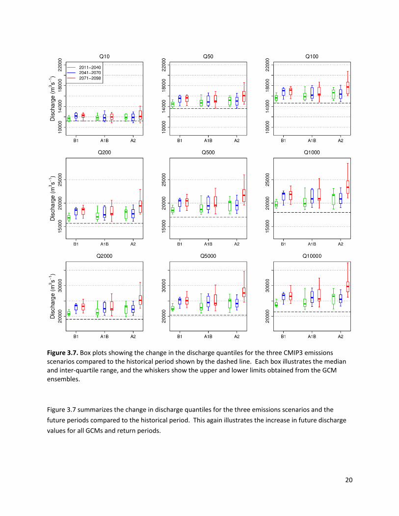
Figure 3.7. Box plots showing the change in the discharge quantiles for the three CMIP3 emissions scenarios compared to the historical period shown by the dashed line. Each box illustrates the median and inter-quartile range, and the whiskers show the upper and lower limits obtained from the GCM ensembles.
Figure 3.7 summarizes the change in discharge quantiles for the three emissions scenarios and the
future periods compared to the historical period. This again illustrates the increase in future discharge
values for all GCMs and return periods.
21
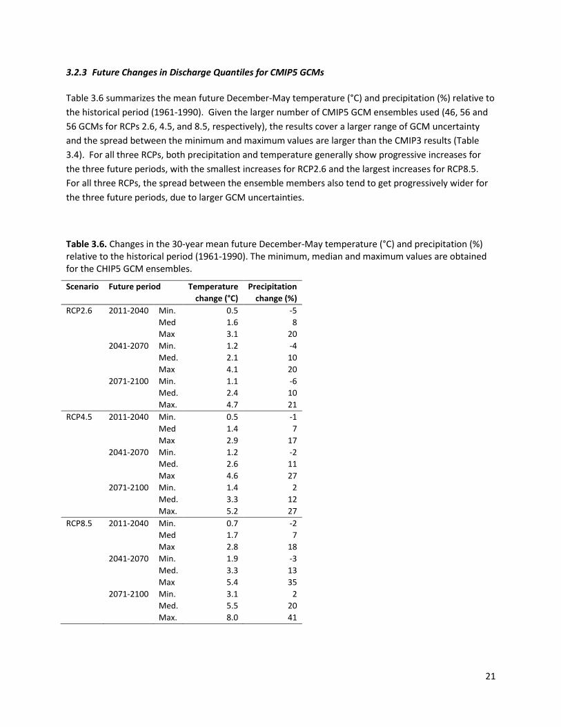
3.2.3 Future Changes in Discharge Quantiles for CMIP5 GCMs
Table 3.6 summarizes the mean future December-May temperature (°C) and precipitation (%) relative to
the historical period (1961-1990). Given the larger number of CMIP5 GCM ensembles used (46, 56 and
56 GCMs for RCPs 2.6, 4.5, and 8.5, respectively), the results cover a larger range of GCM uncertainty
and the spread between the minimum and maximum values are larger than the CMIP3 results (Table
3.4). For all three RCPs, both precipitation and temperature generally show progressive increases for
the three future periods, with the smallest increases for RCP2.6 and the largest increases for RCP8.5.
For all three RCPs, the spread between the ensemble members also tend to get progressively wider for
the three future periods, due to larger GCM uncertainties.
Table 3.6. Changes in the 30-year mean future December-May temperature (°C) and precipitation (%) relative to the historical period (1961-1990). The minimum, median and maximum values are obtained for the CHIP5 GCM ensembles.
Scenario Future period Temperature
change (°C)
Precipitation
change (%)
RCP2.6 2011-2040 Min. 0.5 -5
Med 1.6 8
Max 3.1 20
2041-2070 Min. 1.2 -4
Med. 2.1 10
Max 4.1 20
2071-2100 Min. 1.1 -6
Med. 2.4 10
Max. 4.7 21
RCP4.5 2011-2040 Min. 0.5 -1
Med 1.4 7
Max 2.9 17
2041-2070 Min. 1.2 -2
Med. 2.6 11
Max 4.6 27
2071-2100 Min. 1.4 2
Med. 3.3 12
Max. 5.2 27
RCP8.5 2011-2040 Min. 0.7 -2
Med 1.7 7
Max 2.8 18
2041-2070 Min. 1.9 -3
Med. 3.3 13
Max 5.4 35
2071-2100 Min. 3.1 2
Med. 5.5 20
Max. 8.0 41
22
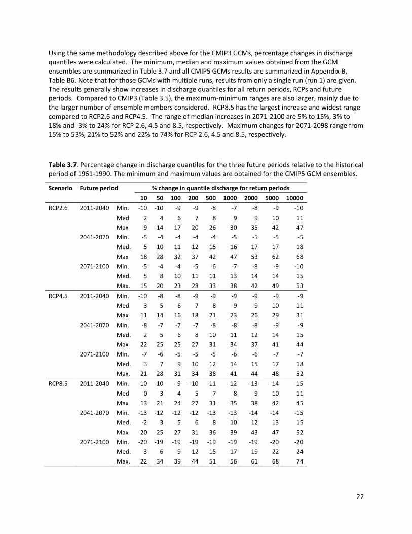
Using the same methodology described above for the CMIP3 GCMs, percentage changes in discharge quantiles were calculated. The minimum, median and maximum values obtained from the GCM ensembles are summarized in Table 3.7 and all CMIP5 GCMs results are summarized in Appendix B, Table B6. Note that for those GCMs with multiple runs, results from only a single run (run 1) are given. The results generally show increases in discharge quantiles for all return periods, RCPs and future periods. Compared to CMIP3 (Table 3.5), the maximum-minimum ranges are also larger, mainly due to the larger number of ensemble members considered. RCP8.5 has the largest increase and widest range compared to RCP2.6 and RCP4.5. The range of median increases in 2071-2100 are 5% to 15%, 3% to 18% and -3% to 24% for RCP 2.6, 4.5 and 8.5, respectively. Maximum changes for 2071-2098 range from 15% to 53%, 21% to 52% and 22% to 74% for RCP 2.6, 4.5 and 8.5, respectively.
Table 3.7. Percentage change in discharge quantiles for the three future periods relative to the historical period of 1961-1990. The minimum and maximum values are obtained for the CMIP5 GCM ensembles.
Scenario Future period % change in quantile discharge for return periods
10 50 100 200 500 1000 2000 5000 10000
RCP2.6 2011-2040 Min. -10 -10 -9 -9 -8 -7 -8 -9 -10
Med 2 4 6 7 8 9 9 10 11
Max 9 14 17 20 26 30 35 42 47
2041-2070 Min. -5 -4 -4 -4 -4 -5 -5 -5 -5
Med. 5 10 11 12 15 16 17 17 18
Max 18 28 32 37 42 47 53 62 68
2071-2100 Min. -5 -4 -4 -5 -6 -7 -8 -9 -10
Med. 5 8 10 11 11 13 14 14 15
Max. 15 20 23 28 33 38 42 49 53
RCP4.5 2011-2040 Min. -10 -8 -8 -9 -9 -9 -9 -9 -9
Med 3 5 6 7 8 9 9 10 11
Max 11 14 16 18 21 23 26 29 31
2041-2070 Min. -8 -7 -7 -7 -8 -8 -8 -9 -9
Med. 2 5 6 8 10 11 12 14 15
Max 22 25 25 27 31 34 37 41 44
2071-2100 Min. -7 -6 -5 -5 -5 -6 -6 -7 -7
Med. 3 7 9 10 12 14 15 17 18
Max. 21 28 31 34 38 41 44 48 52
RCP8.5 2011-2040 Min. -10 -10 -9 -10 -11 -12 -13 -14 -15
Med 0 3 4 5 7 8 9 10 11
Max 13 21 24 27 31 35 38 42 45
2041-2070 Min. -13 -12 -12 -12 -13 -13 -14 -14 -15
Med. -2 3 5 6 8 10 12 13 15
Max 20 25 27 31 36 39 43 47 52
2071-2100 Min. -20 -19 -19 -19 -19 -19 -19 -20 -20
Med. -3 6 9 12 15 17 19 22 24
Max. 22 34 39 44 51 56 61 68 74
23
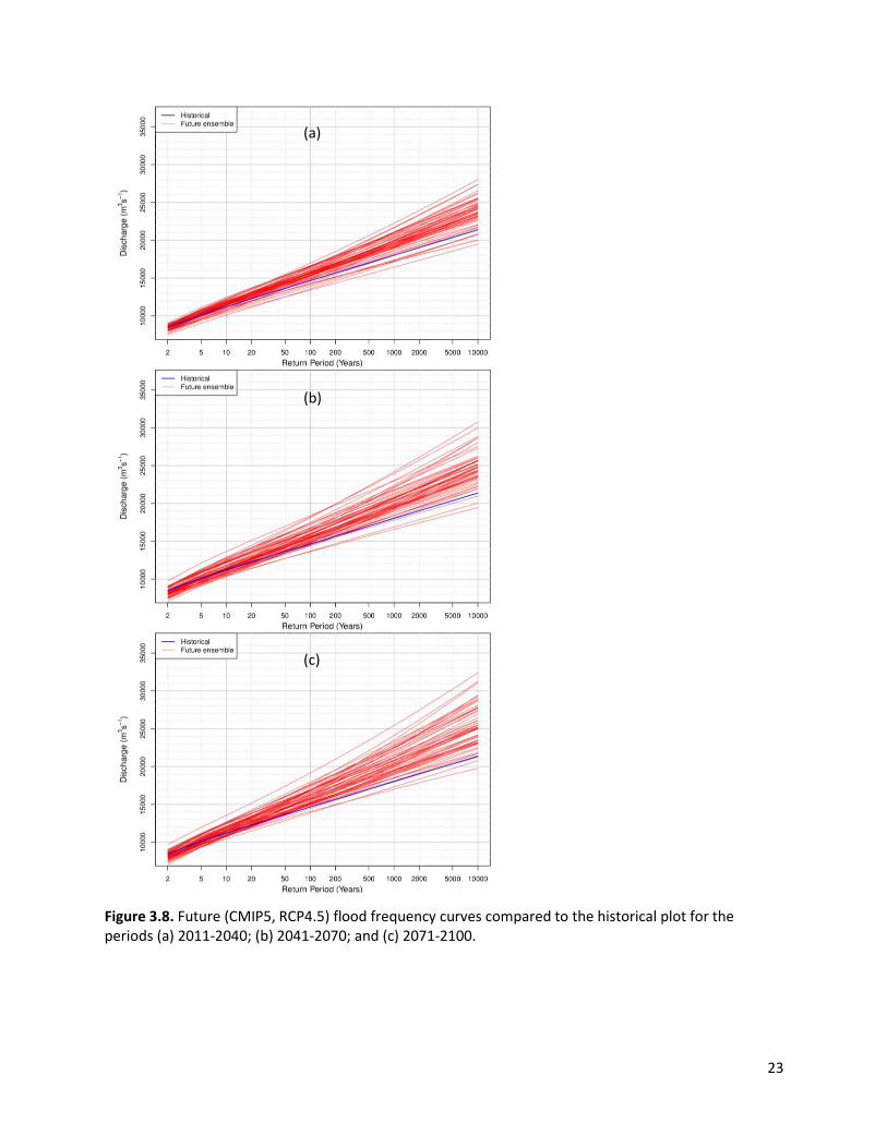
Figure 3.8. Future (CMIP5, RCP4.5) flood frequency curves compared to the historical plot for the periods (a) 2011-2040; (b) 2041-2070; and (c) 2071-2100.
(a)
(b)
(c)
24
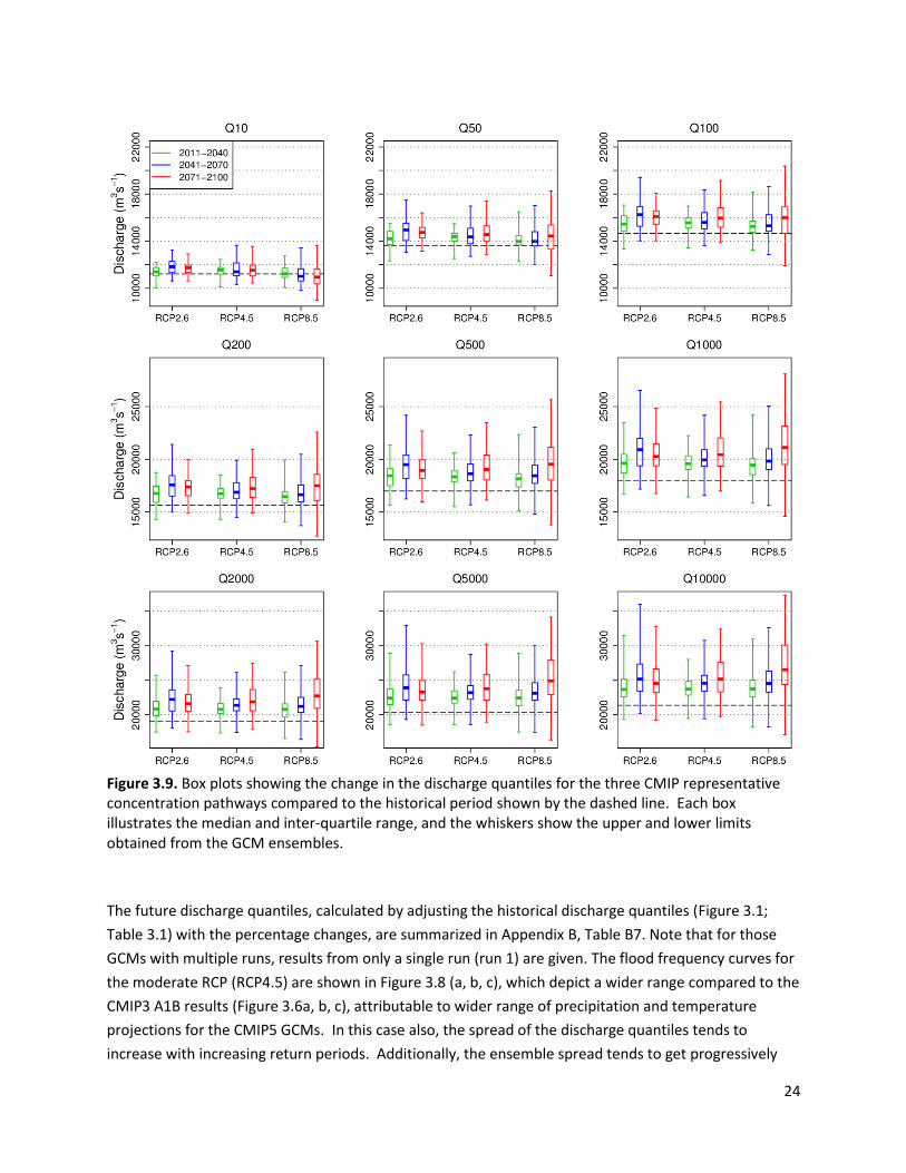
Figure 3.9. Box plots showing the change in the discharge quantiles for the three CMIP representative concentration pathways compared to the historical period shown by the dashed line. Each box illustrates the median and inter-quartile range, and the whiskers show the upper and lower limits obtained from the GCM ensembles.
The future discharge quantiles, calculated by adjusting the historical discharge quantiles (Figure 3.1;
Table 3.1) with the percentage changes, are summarized in Appendix B, Table B7. Note that for those
GCMs with multiple runs, results from only a single run (run 1) are given. The flood frequency curves for
the moderate RCP (RCP4.5) are shown in Figure 3.8 (a, b, c), which depict a wider range compared to the
CMIP3 A1B results (Figure 3.6a, b, c), attributable to wider range of precipitation and temperature
projections for the CMIP5 GCMs. In this case also, the spread of the discharge quantiles tends to
increase with increasing return periods. Additionally, the ensemble spread tends to get progressively

25
wider for 2011-2040, 2041-2070 and 2071-2100. The frequency curves for the RCP2.6 and RCP8.5 are
available in Appendix C, Figures C3 and C4, respectively.
Figure 3.9 summarizes the future discharge quantiles for the three RCPs compared to the historical
period. The results depict a tendency for increased quantile discharges in the future. Specifically,
although several individual projections indicate decreased quantile values, the ensemble median values
generally show progressively increasing quantile values for the three future periods for all return periods
(excepting T=10 years). An exception to this is RCP2.6 scenario, which shows the quantile values
peaking in mid-century (2014-2070), which is a consequence of the emissions for this RCP also peaking
in mid-century (see Appendix A for a description of emissions scenarios).
3.2.4 Uncertainties in Estimating Discharge Quantiles
Uncertainty is an inherent in the development of hydrologic projections. The quantification of projected
changes in annual maximum peak flow quantiles based on the methodology employed is affected by the
following main sources of uncertainty:
1. Choice of emissions scenario;
2. GCM structure;
3. Climate variability;
4. Hydrologic model and GEVcdn model structure; and
5. Sampling variability.
Climate projections are affected by uncertainties arising from the unknown trajectory of future
greenhouse gas (GHG) emissions, GCM model structure, natural variability of the climate system, and
choice of downscaling method (Kay et al. 2008). Previous studies (Kay et al. 2008; Prudhomme and
Davies 2008a,b; Bennett et al. 2012) indicated that, in the context of hydrologic projections, GCM
structure is the largest source of uncertainty. The climate’s natural chaotic internal variability, which is
represented by ensemble members of a climate model, can also have appreciable impacts on the
sensitivity of some of the outputs (Kendon et al. 2010; Deser et al. 2012). For the CMIP5-based
projections the uncertainties related to the GHG emissions, GCM structure and natural climate
variability have been explicitly taken into account by using a large ensemble of different GCMs with
multiple runs (for select GCMs) for a range of emissions scenarios. It is to be noted that the CMIP3-
based projections use a much more limited number of GCMs, with only a single run from each model
(ensemble size of 7, 8 and 8 for B1, A1B and A2, respectively). Hence, projection uncertainty is likely
underestimated for the CMIP3 results. Nevertheless, this is not considered problematic as the CMIP3-
based climate projections are primarily used for training and validation of the GEVcdn model.
Uncertainty due to downscaling has not been explicitly addressed, but is expected to be a minor
component of overall climate projection uncertainty.
The VIC model simulated CMIP3 streamflow used for setting up the GEVcdn model is also affected by
uncertainties. Specifically, hydrologic models are affected by errors in input data, model structure, and
26
parameter specification (Beven 2006). These errors affect the ability of a hydrologic model in replicating
the observed variability of streamflow, including streamflow extremes (Shrestha et al. 2014). However,
the use of a simple scaling approach to estimate future discharge quantiles (i.e. the ‘observed’ peak flow
frequency is scaled according to quantile changes modelled using GEVcdn) is expected to mitigate the
effect of any VIC model bias in simulating annual maximum peak flow. The application of the GEVcdn
methodology for estimating future discharge is also subject to uncertainty. Firstly, the chosen
covariates may not fully describe the mechanism for generation of annual maximum peak streamflows
and, secondly, given the limited extrapolation capability of a neural network, the GEVcdn model is not
suitable for estimating discharge quantiles beyond the range of training dataset. However, model
verification (see Section 3.2.1) indicates that the GEVcdn model is accurate and robust and the CMIP5
climate projections are within the range of the CMIP3 training data. VIC- and GEVcdn-related errors and
uncertainties are judged to be relatively minor with respect to the uncertainties in the climate
projections.
Lastly, GEV parameter estimation (for both stationary and nonstationary parameters) is also affected by
uncertainties due to sampling variability (Kharin and Zwiers 2005). In particular, the effect of sampling
variability can be considerable for the longer return period flow quantiles (e.g., > 1000 years). As such
we advise caution when using peak discharge values reported herein for such high return period (low
probability) events.
27
4. CONCLUSIONS AND FUTURE WORK
This study evaluated potential future changes in flood frequencies for the Fraser River at Hope station
(WSC gauge 08MF005). The analysis was conducted using the GEV conditional density network
(GEVcdn) statistical model, which provides a flexible, efficient and robust means of estimating the
nonstationary distribution of annual maximum streamflow events using the Generalized Extreme Value
(GEV) distribution. Results are presented for a range of possible future emission scenarios spanning low,
medium and high emission (e.g. CMIP3) or strong mitigation, stabilization or high emissions (i.e.
business-as-usual; CMIP5) using output from a large pool of GCMs derived from two separate global
climate modelling experiments. Although not explicitly predictions of the future, the provided
projections cover wide and realistic range of possible future outcomes and, hence, will prove useful for
flood management and adaptation activities.
In the first part of this work, a stationary analysis of extreme historical discharge was conducted based
on 102-year (1912-2013) historical peak annual maximum daily flow data, supplemented with estimated
1894 peak discharge value. Based on the fitted Gumbel distribution, the 1894 event (≈ 17000 m3/s) has
a return period of about 500 years, with a 16000 m3/s to 18000 m3/s confidence range (5% to 95%).
Alternatively, a 17000 m3/s event is estimated to have a return period ranging from 250 to 1000 years
(also based on 5% to 95% confidence range). .
In the second part of this study, a nonstationary analysis of the VIC model simulated historical/future
discharge was conducted with the GEV parameters expressed as a function of covariates. The GEV
conditional density network (GEVcdn) was employed for the estimation of GEV parameters, with
covariates consisting of seasonal precipitation and temperature from CMIP3 and time (year). The
results of the GEVcdn nonstationary model showed a good ability of the model to simulate quantile
discharges and a reasonable representation of the temporal patterns in the VIC simulated streamflow
extremes. The results also illustrate high inter-annual variability in the parameters of the GEV
distribution. Thus, for the evaluation of the climate driven changes in streamflow extremes, we used
30-year climatological periods, which we treated as stationary, and evaluated future change in discharge
quantiles relative to the discharge quantiles from a baseline historical period. Results of the analysis
showed increases in flow quantiles for both the CMIP3- and CMIP5-based projections, with progressively
larger increases for 2011-2040, 2041-2070 and 2071-2100. The median increases in 2071-2098 based
on CMIP3 GCM ensembles are 9% to 24%, 7% to 20% and 8% to 39% (range are for 10 year-10000 year
return periods) for B1, A1B and A2 scenarios, respectively. The maximum increases in 2071-2098 from
CMIP3 GCM ensembles are 14% to 41%, 15% to 52% and 25% to 75% for B1, A1B and A2 scenarios,
respectively. In the case of CMIP5 GCM ensembles, the range of median increases in 2071-2100 are 5%
to 15%, 3% to 18% and -3% to 24% for RCP 2.6, 4.5 and 8.5, respectively. The maximum increase ranges
are 15% to 53%, 21% to 52% and 22% to 74% for RCP 2.6, 4.5 and 8.5, respectively.
The results of this study are affected by a number of different sources of uncertainties, which arise from
emissions uncertainty, model structure, and climate variability. The methodology of using projection
ensembles based on a range of possible emission, multiple GCMs, and multiple runs per GCM explicitly
and addresses uncertainty in the climate projections. However, long return period events (e.g. > 1000
28
year) are particularly affected by uncertainties due to sampling variability, and the results for long return
period events presented in this report should be treated with a caution.
For future research, the streamflow extremes for CMIP5 should be updated with the CMIP5 GCM driven
VIC model simulations. While the GEVcdn model provides a robust statistical methodology for
evaluating the parameters of the GEV distribution based on climatic covariates, the CMIP5 GCM driven
VIC simulations will provide a means for directly estimating the GEV parameters for future peak flow
distributions. The generation of hydrologic projections using the VIC model is part of PCIC’s work plan,
but the process is resource intensive and will likely require several years. Nevertheless, the use of such
direct methodology could potentially reduce uncertainties in the projected streamflow extremes. Future
research should also focus on ascertaining a clearer understanding of the physical mechanisms which
drive annual maximum peak flow events, particularly extremely rare events. A more physically-based
understanding of peak flow change would lend greater confidence to climate change studies on flood
impacts.
29
REFERENCES
Akaike, H., 1974: A new look at the statistical model identification. IEEE Trans. Autom. Control, 19, 716–723, doi:10.1109/TAC.1974.1100705.
Arora, V. K., and Coauthors, 2011: Carbon emission limits required to satisfy future representative concentration pathways of greenhouse gases. Geophys. Res. Lett., 38, n/a – n/a, doi:10.1029/2010GL046270.
Bennett, K. E., A. T. Werner, and M. Schnorbus, 2012: Uncertainties in Hydrologic and Climate Change Impact Analyses in Headwater Basins of British Columbia. J. Clim., 25, 5711–5730, doi:10.1175/JCLI-D-11-00417.1.
Beven, K., 2006: A manifesto for the equifinality thesis. J. Hydrol., 320, 18–36, doi:10.1016/j.jhydrol.2005.07.007.
Cannon, A. J., 2010: A flexible nonlinear modelling framework for nonstationary generalized extreme value analysis in hydroclimatology. Hydrol. Process., 24, 673–685, doi:10.1002/hyp.7506.
——, 2011: GEVcdn: An R package for nonstationary extreme value analysis by generalized extreme value conditional density estimation network. Comput. Geosci., 37, 1532–1533, doi:10.1016/j.cageo.2011.03.005.
——, 2014: GEVcdn: GEV conditional density estimation network. http://cran.r-project.org/web/packages/GEVcdn/index.html (Accessed January 22, 2015).
Coles, S., 2001: An Introduction to Statistical Modeling of Extreme Values. Springer Science & Business Media, 226 pp.
Condon, L. E., S. Gangopadhyay, and T. Pruitt, 2015: Climate change and non-stationary flood risk for the upper Truckee River basin. Hydrol Earth Syst Sci, 19, 159–175, doi:10.5194/hess-19-159-2015.
Cooley, D., 2013: Return Periods and Return Levels Under Climate Change. Extremes in a Changing Climate, A. AghaKouchak, D. Easterling, K. Hsu, S. Schubert, and S. Sorooshian, Eds., Water Science and Technology Library, Springer Netherlands, 97–114 http://link.springer.com/chapter/10.1007/978-94-007-4479-0_4 (Accessed April 17, 2015).
Deser, C., A. Phillips, V. Bourdette, and H. Teng, 2012: Uncertainty in climate change projections: the role of internal variability. Clim. Dyn., 38, 527–546, doi:10.1007/s00382-010-0977-x.
Edenhofer, O., and Coauthors, eds., 2014: Climate change 2014: Mitigation of climate change. Work. Group III Contrib. Fifth Assess. Rep. Intergov. Panel Clim. Change UK N. Y.,. http://report.mitigation2014.org/spm/ipcc_wg3_ar5_summary-for-policymakers_may-version.pdf (Accessed April 22, 2015).
Flood Safety Section, 2014: Simulating the Effects of Sea Level Rise and Climate Change on Fraser River Flood Scenarios. BC Ministry of Forests, Lands and Natural Resource Operations, Surrey, BC, http://www.env.gov.bc.ca/wsd/public_safety/flood/pdfs_word/Simulating_Effects_of_Sea_Level_Rise_and_Climate_Change_on_Fraser_Flood_Scenarios_Final_Report_May-2014.pdf.
30
Friederichs, P., and A. Hense, 2007: Statistical Downscaling of Extreme Precipitation Events Using Censored Quantile Regression. Mon. Weather Rev., 135, 2365–2378, doi:10.1175/MWR3403.1.
Friederichs, P., and A. Hense, 2008: A Probabilistic Forecast Approach for Daily Precipitation Totals. Weather Forecast., 23, 659–673, doi:10.1175/2007WAF2007051.1.
Hirsch, R. M., and J. R. Stedinger, 1987: Plotting positions for historical floods and their precision. Water Resour. Res., 23, 715–727, doi:10.1029/WR023i004p00715.
Huntington, T. G., 2006: Evidence for intensification of the global water cycle: Review and synthesis. J. Hydrol., 319, 83–95, doi:10.1016/j.jhydrol.2005.07.003.
Hurvich, C. M., and C.-L. Tsai, 1989: Regression and time series model selection in small samples. Biometrika, 76, 297–307, doi:10.1093/biomet/76.2.297.
Katz, R. W., 2013: Statistical Methods for Nonstationary Extremes. Extremes in a Changing Climate, A. AghaKouchak, D. Easterling, K. Hsu, S. Schubert, and S. Sorooshian, Eds., Water Science and Technology Library, Springer Netherlands, 15–37 http://link.springer.com/chapter/10.1007/978-94-007-4479-0_2 (Accessed January 21, 2015).
Kay, A. L., H. N. Davies, V. A. Bell, and R. G. Jones, 2008: Comparison of uncertainty sources for climate change impacts: flood frequency in England. Clim. Change, 92, 41–63, doi:10.1007/s10584-008-9471-4.
Kendon, E. J., R. G. Jones, E. Kjellström, and J. M. Murphy, 2010: Using and Designing GCM–RCM Ensemble Regional Climate Projections. J. Clim., 23, 6485–6503, doi:10.1175/2010JCLI3502.1.
Kharin, V. V., and F. W. Zwiers, 2005: Estimating Extremes in Transient Climate Change Simulations. J. Clim., 18, 1156–1173, doi:10.1175/JCLI3320.1.
Kharin, V. V., F. W. Zwiers, X. Zhang, and M. Wehner, 2013: Changes in temperature and precipitation extremes in the CMIP5 ensemble. Clim. Change, 119, 345–357, doi:10.1007/s10584-013-0705-8.
Knutti, R., and J. Sedláček, 2013: Robustness and uncertainties in the new CMIP5 climate model projections. Nat. Clim. Change, 3, 369–373, doi:10.1038/nclimate1716.
Moss, R. H., and Coauthors, 2008: Towards New Scenarios for Analysis of Emissions, Climate Change, Impacts, and Response Strategies. Pacific Northwest National Laboratory (PNNL), Richland, WA (US), http://www.osti.gov/scitech/biblio/940991 (Accessed April 22, 2015).
——, and Coauthors, 2010: The next generation of scenarios for climate change research and assessment. Nature, 463, 747–756, doi:10.1038/nature08823.
Nakićenović, N., and R. Swart, eds., 2000: Special report on emissions scenarios: a special report of working group III of the Intergovernmental Panel on Climate Change. Cambridge University Press,.
Northwest Hydraulic Consultants, 2008: Comprehensive review of Fraser at Hope flood hydrology and flows - Scoping Study. Surrey, BC,
31
http://www.env.gov.bc.ca/wsd/public_safety/flood/pdfs_word/review_fraser_flood_flows_hope.pdf.
Payrastre, O., E. Gaume, and H. Andrieu, 2011: Usefulness of historical information for flood frequency analyses: Developments based on a case study. Water Resour. Res., 47, W08511, doi:10.1029/2010WR009812.
Phien, H. N., 1987: A review of methods of parameter estimation for the extreme value type-1 distribution. J. Hydrol., 90, 251–268, doi:10.1016/0022-1694(87)90070-9.
Prudhomme, C., and H. Davies, 2008a: Assessing uncertainties in climate change impact analyses on the river flow regimes in the UK. Part 2: future climate. Clim. Change, 93, 197–222, doi:10.1007/s10584-008-9461-6.
——, and ——, 2008b: Assessing uncertainties in climate change impact analyses on the river flow regimes in the UK. Part 2: future climate. Clim. Change, 93, 197–222, doi:10.1007/s10584-008-9461-6.
Salas, J., and J. Obeysekera, 2014: Revisiting the Concepts of Return Period and Risk for Nonstationary Hydrologic Extreme Events. J. Hydrol. Eng., 19, 554–568, doi:10.1061/(ASCE)HE.1943-5584.0000820.
Schnorbus, M., A. Werner, and K. Bennett, 2014: Impacts of climate change in three hydrologic regimes in British Columbia, Canada. Hydrol. Process., 28, 1170–1189, doi:10.1002/hyp.9661.
Schnorbus, M. A., and A. J. Cannon, 2014: Statistical emulation of streamflow projections from a distributed hydrological model: Application to CMIP3 and CMIP5 climate projections for British Columbia, Canada. Water Resour. Res., n/a – n/a, doi:10.1002/2014WR015279.
Shrestha, R. R., M. A. Schnorbus, A. T. Werner, and A. J. Berland, 2012: Modelling spatial and temporal variability of hydrologic impacts of climate change in the Fraser River basin, British Columbia, Canada. Hydrol. Process., 26, 1840–1860, doi:10.1002/hyp.9283.
——, D. L. Peters, and M. A. Schnorbus, 2014: Evaluating the ability of a hydrologic model to replicate hydro-ecologically relevant indicators. Hydrol. Process., 28, 4294–4310, doi:10.1002/hyp.9997.
Solomon, S., D. Qin, M. Manning, Z Chen, M. Marquis, K. Averyt, M. Tignor, and Miller, eds., 2007: Climate change 2007-the physical science basis: Working group I contribution to the fourth assessment report of the IPCC. Cambridge University Press,.
Stedinger, J. R., R. M. Vogel, and E. Foufoula-Georgiou, 1993: Frequency analysis of extreme events. Handbook of Hydrology, D.R. Maidment, Ed., McGraw-Hill, United States, p. 1424.
Towler, E., B. Rajagopalan, E. Gilleland, R. S. Summers, D. Yates, and R. W. Katz, 2010: Modeling hydrologic and water quality extremes in a changing climate: A statistical approach based on extreme value theory. Water Resour. Res., 46, W11504, doi:10.1029/2009WR008876.
32
Vasiliades, L., P. Galiatsatou, and A. Loukas, 2014: Nonstationary Frequency Analysis of Annual Maximum Rainfall Using Climate Covariates. Water Resour. Manag., 29, 339–358, doi:10.1007/s11269-014-0761-5.
Van Vuuren, D. P., and Coauthors, 2011: The representative concentration pathways: an overview. Clim. Change, 109, 5–31, doi:10.1007/s10584-011-0148-z.
Wilks, D. S., 2006: Statistical Methods in the Atmospheric Sciences: An Introduction. Academic Press, 650 pp.
Zhang, X., J. Wang, F. W. Zwiers, and P. Y. Groisman, 2010: The Influence of Large-Scale Climate Variability on Winter Maximum Daily Precipitation over North America. J. Clim., 23, 2902–2915, doi:10.1175/2010JCLI3249.1.
33
LIST OF TABLES
Table 3.1. L-moment Gumbel parameter estimates .................................................................................. 11
Table 3.2. GEV Type I Distribution Quantile Estimates for the Fraser River at Hope ................................. 12
Table 3.3. Range of GEV parameters obtained from the GEVcdn model (iv) ............................................. 14
Table 3.4. Changes in the 30-year mean (28-year for 2071-2098) future December-May temperature (°C)
and precipitation (%) relative to the historical period (1961-1990). The minimum, median and maximum
values are obtained for the CHIP3 GCM ensembles. .................................................................................. 17
Table 3.5. Percentage change in discharge quantiles for the three future periods relative to the historical
period of 1961-1990. The minimum, median and maximum values are obtained from the CHIP3 GCM
ensembles. .................................................................................................................................................. 18
Table 3.6. Changes in the 30-year mean future December-May temperature (°C) and precipitation (%)
relative to the historical period (1961-1990). The minimum, median and maximum values are obtained
for the CHIP5 GCM ensembles. ................................................................................................................... 21
Table 3.7. Percentage change in discharge quantiles for the three future periods relative to the historical
period of 1961-1990. The minimum and maximum values are obtained for the CHIP5 GCM ensembles. 22
Table B1. Annual maximum flow data and plotting positions for Fraser River at Hope (WSC 08MF005) . 38
Table B2. Summary of CMIP3 Global Climate Model ensemble ................................................................ 41
Table B3. Summary of CMIP5 Global Climate Model ensemble ................................................................ 42
Table B4. Percentage change in discharge quantiles for the three future periods against the historical
period of 1961-1990. The results are for CMIP3 GCMs. ............................................................................. 43
Table B5. Discharge quantiles for the three future periods for the CMIP3 GCMs. .................................... 45
Table B6. Percentage change in discharge quantiles for the three future periods against the historical
period of 1961-1990. The results are for selected CMIP5 GCMs ............................................................... 47
Table B7. Discharge quantiles for the three future periods for the selected CMIP5 GCMs. ...................... 50
34
LIST OF FIGURES
Figure 2.1. Time series of annual maximum peak discharge for the Fraser River at Hope, showing both
instrumental and documentary discharge values. ....................................................................................... 5
Figure 2.2. Structure of the GEVcdn model (adapted from Cannon 2010). The dashed lines connecting
output node 𝝃 show inactive connections when 𝝃 is considered constant. ................................................. 8
Figure 3.1. Plotting positions of observed and estimated historical events with fitted GEV Type I
distributions showing discharge as a function of return period. Bottom axis shows the return period, as
well as the non-exceedance probability. .................................................................................................... 12
Figure 3.2. Plotting positions of observed and estimated historical events with fitted GEV Type I
distributions showing return period as a function of discharge. Left axis shows the return period, as well
as the non-exceedance probability. ............................................................................................................ 13
Figure 3.3. QVSS for (a) training and (b) validation datasets for four the combination of covariates: (i)
winter and spring precipitation, and spring temperature (djf P, mam P, mam T); (ii) winter and spring
precipitation, spring temperature and year (djf P, mam P, mam T, Y); (iii) winter and spring precipitation,
winter and spring temperature (djf P, mam P, djf T, mam T); (iv) winter and spring precipitation, winter
and spring temperature and time (djf P, mam P, djf T, mam T, Y). ............................................................ 14
Figure 3.4. Quantile-quantile plots of VIC simulated results and a random realization GEVcdn model for
(a) training and (b) validation datasets. The red line shows the one-to-one relationship. ....................... 15
Figure 3.5. 95th and 5th percentiles envelopes from the GEVcdn model obtained from CMIP3-based GCM
ensembles for the 2-year, 10-year and 100-year return period discharges for (a) training and (b)
validation datasets. The grey crosses represent the VIC simulated peak flows for the corresponding
GCMs. Training is based on the B1 and A1B emissions scenarios, validation is based on the A2 scenario.
.................................................................................................................................................................... 16
Figure 3.6. Future (CMIP3 A1B emissions scenario) flood frequency curves compared to the historical
plot for the periods (a) 2011-2040; (b) 2041-2070; and (c) 2071-2098. .................................................... 19
Figure 3.7. Box plots showing the change in the discharge quantiles for the three CMIP3 emissions
scenarios compared to the historical period shown by the dashed line. Each box illustrates the median
and inter-quartile range, and the whiskers show the upper and lower limits obtained from the GCM
ensembles. .................................................................................................................................................. 20
Figure 3.8. Future (CMIP5, RCP4.5) flood frequency curves compared to the historical plot for the
periods (a) 2011-2040; (b) 2041-2070; and (c) 2071-2100. ........................................................................ 23
Figure 3.9. Box plots showing the change in the discharge quantiles for the three CMIP representative
concentration pathways compared to the historical period shown by the dashed line. Each box
illustrates the median and inter-quartile range, and the whiskers show the upper and lower limits
obtained from the GCM ensembles. ........................................................................................................... 24
Figure A1. Global temperature change and uncertainty. Global temperature change (mean and one
standard deviation as shading) relative to 1986–2005 for the SRES scenarios run by CMIP3 and the RCP
scenarios run by CMIP5. The number of models is given in brackets. The box plots (mean, one standard
deviation, and minimum to maximum range) are given for 2080–2099 for CMIP5 (colours) and for the
35
model calibrated to 19 CMIP3 models (black), both running the RCP scenarios (Source: Knutti and
Sedláček 2013). ........................................................................................................................................... 37
Figure C1. Future (CMIP3 B1 emissions scenarios) flood frequency curves compared to the historical plot
for the periods (a) 2011-2040; (b) 2041-2070; and (c) 2071-2100. ............................................................ 54
Figure C2. . Future (CMIP3 A2 emissions scenarios) flood frequency curves compared to the historical
plot for the periods (a) 2011-2040; (b) 2041-2070; and (c) 2071-2100. .................................................... 55
Figure C3. Future (CMIP5 RCP2.6) flood frequency curves compared to the historical plot for the periods
(a) 2011-2040; (b) 2041-2070; and (c) 2071-2100. ..................................................................................... 56
Figure C4. . Future (CMIP5 RCP8.5) flood frequency curves compared to the historical plot for the
periods (a) 2011-2040; (b) 2041-2070; and (c) 2071-2100 ......................................................................... 57
36
APPENDIX A: EMISSIONS SCENARIOS
A1. Special Report on Emissions Scenarios (SRES)
SRES scenarios are emission scenarios, developed by Nakićenović and Swart (2000), are used as the basis
for climate projections for phase 3 of the Coupled Model Intercomparison Project (CMIP3). A brief
description of the SRES scenarios from Nakićenović and Swart (2000), which are used in this report is
given below:
The A1 storyline and scenario family describes a future world of very rapid economic growth,
global population that peaks in mid-century and declines thereafter, and the rapid introduction
of new and more efficient technologies. Major underlying themes are convergence among
regions, capacity building, and increased cultural and social interactions, with a substantial
reduction in regional differences in per capita income. The A1 scenario family develops into
three groups that describe alternative directions of technological change in the energy system.
The three A1 groups are distinguished by their technological emphasis: fossil intensive (A1FI),
non-fossil energy sources (A1T), or a balance across all sources (A1B).
The B1 storyline and scenario family describes a convergent world with the same global
population that peaks in mid-century and declines thereafter, as in the A1 storyline, but with
rapid changes in economic structures toward a service and information economy, with
reductions in material intensity, and the introduction of clean and resource-efficient
technologies. The emphasis is on global solutions to economic, social, and environmental
sustainability, including improved equity, but without additional climate initiatives.
The A2 storyline and scenario family describes a very heterogeneous world. The underlying
theme is self-reliance and preservation of local identities. Fertility patterns across regions
converge very slowly, which results in continuously increasing global population. Economic
development is primarily regionally oriented and per capita economic growth and technological
change are more fragmented and slower than in other storylines.
A2. Representative Concentration Pathways (RCPs)
The RCP emissions scenarios provide the radiative forcing conditions for phase 5 of the Coupled Model
Intercomparison Project (CMIP5). RCP scenarios include time series of emissions and concentrations of
the full suite of greenhouse gases (GHGs) and aerosols and chemically active gases, as well as land use /
land cover (Moss et al. 2008). The word representative signifies that each RCP provides only one of
many possible scenarios that would lead to the specific radiative forcing characteristics. The term
pathway emphasizes that not only the long-term concentration levels are of interest, but also the
trajectory taken over time to reach that outcome (Moss et al. 2010). A brief description of the RCPs from
IPCC WGIII Glossary (Edenhofer et al. 2014), which are used in this report is given below:
RCP2.6 is a pathway where radiative forcing peaks at approximately 3 W m-2 before 2100 and
then declines.
RCP4.5 is an intermediate stabilization pathway in which radiative forcing is stabilized at
approximately 4.5 W m-2 after 2100.
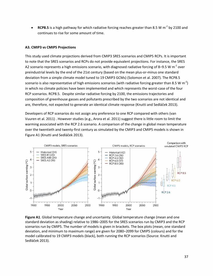
37
RCP8.5 is a high pathway for which radiative forcing reaches greater than 8.5 W m-2 by 2100 and
continues to rise for some amount of time.
A3. CMIP3 vs CMIP5 Projections
This study used climate projections derived from CMIP3 SRES scenarios and CMIP5 RCPs. It is important
to note that the SRES scenarios and RCPs do not provide equivalent projections. For instance, the SRES
A2 scenario represents a high emissions scenario, with diagnosed radiative forcing of 8–9.5 W m-2 over
preindustrial levels by the end of the 21st century (based on the mean plus-or-minus one standard
deviation from a simple climate model tuned to 19 CMIP3 GCMs) (Solomon et al. 2007). The RCP8.5
scenario is also representative of high emissions scenarios (with radiative forcing greater than 8.5 W m-2)
in which no climate policies have been implemented and which represents the worst-case of the four
RCP scenarios. RCP8.5. Despite similar radiative forcing by 2100, the emissions trajectories and
composition of greenhouse gasses and pollutants prescribed by the two scenarios are not identical and
are, therefore, not expected to generate an identical climate response (Knutti and Sedláček 2013).
Developers of RCP scenarios do not assign any preference to one RCP compared with others (van
Vuuren et al. 2011) . However studies (e.g., Arora et al. 2011) suggest there is little room to limit the
warming associated with the RCP 2.6 scenario. A comparison of the change in global mean temperature
over the twentieth and twenty-first century as simulated by the CMIP3 and CMIP5 models is shown in
Figure A1 (Knutti and Sedláček 2013).
Figure A1. Global temperature change and uncertainty. Global temperature change (mean and one standard deviation as shading) relative to 1986–2005 for the SRES scenarios run by CMIP3 and the RCP scenarios run by CMIP5. The number of models is given in brackets. The box plots (mean, one standard deviation, and minimum to maximum range) are given for 2080–2099 for CMIP5 (colours) and for the model calibrated to 19 CMIP3 models (black), both running the RCP scenarios (Source: Knutti and Sedláček 2013).
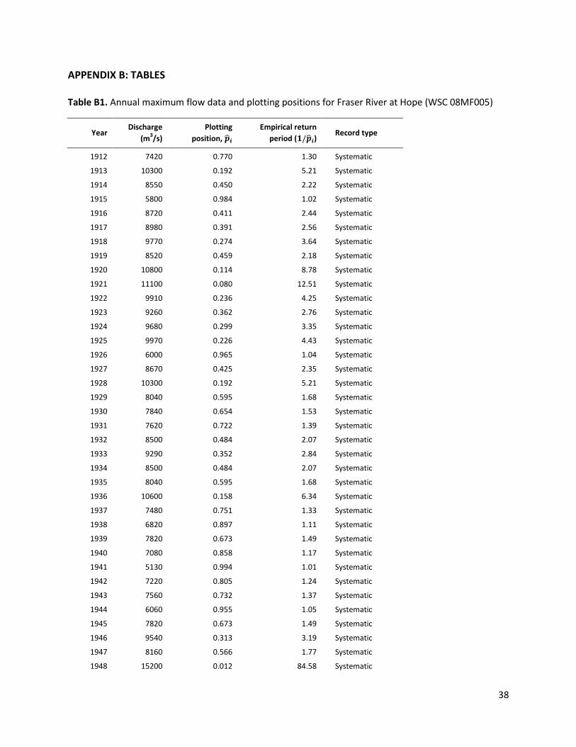
38
APPENDIX B: TABLES
Table B1. Annual maximum flow data and plotting positions for Fraser River at Hope (WSC 08MF005)
Year Discharge
(m3/s)
Plotting
position, �̂�𝒊
Empirical return
period (𝟏/�̂�𝒊) Record type
1912 7420 0.770 1.30 Systematic
1913 10300 0.192 5.21 Systematic
1914 8550 0.450 2.22 Systematic
1915 5800 0.984 1.02 Systematic
1916 8720 0.411 2.44 Systematic
1917 8980 0.391 2.56 Systematic
1918 9770 0.274 3.64 Systematic
1919 8520 0.459 2.18 Systematic
1920 10800 0.114 8.78 Systematic
1921 11100 0.080 12.51 Systematic
1922 9910 0.236 4.25 Systematic
1923 9260 0.362 2.76 Systematic
1924 9680 0.299 3.35 Systematic
1925 9970 0.226 4.43 Systematic
1926 6000 0.965 1.04 Systematic
1927 8670 0.425 2.35 Systematic
1928 10300 0.192 5.21 Systematic
1929 8040 0.595 1.68 Systematic
1930 7840 0.654 1.53 Systematic
1931 7620 0.722 1.39 Systematic
1932 8500 0.484 2.07 Systematic
1933 9290 0.352 2.84 Systematic
1934 8500 0.484 2.07 Systematic
1935 8040 0.595 1.68 Systematic
1936 10600 0.158 6.34 Systematic
1937 7480 0.751 1.33 Systematic
1938 6820 0.897 1.11 Systematic
1939 7820 0.673 1.49 Systematic
1940 7080 0.858 1.17 Systematic
1941 5130 0.994 1.01 Systematic
1942 7220 0.805 1.24 Systematic
1943 7560 0.732 1.37 Systematic
1944 6060 0.955 1.05 Systematic
1945 7820 0.673 1.49 Systematic
1946 9540 0.313 3.19 Systematic
1947 8160 0.566 1.77 Systematic
1948 15200 0.012 84.58 Systematic
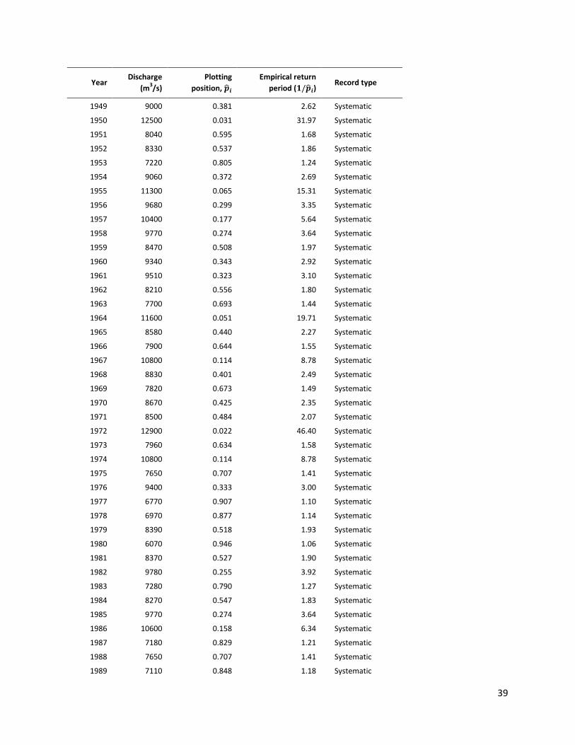
39
Year Discharge
(m3/s)
Plotting
position, �̂�𝒊
Empirical return
period (𝟏/�̂�𝒊) Record type
1949 9000 0.381 2.62 Systematic
1950 12500 0.031 31.97 Systematic
1951 8040 0.595 1.68 Systematic
1952 8330 0.537 1.86 Systematic
1953 7220 0.805 1.24 Systematic
1954 9060 0.372 2.69 Systematic
1955 11300 0.065 15.31 Systematic
1956 9680 0.299 3.35 Systematic
1957 10400 0.177 5.64 Systematic
1958 9770 0.274 3.64 Systematic
1959 8470 0.508 1.97 Systematic
1960 9340 0.343 2.92 Systematic
1961 9510 0.323 3.10 Systematic
1962 8210 0.556 1.80 Systematic
1963 7700 0.693 1.44 Systematic
1964 11600 0.051 19.71 Systematic
1965 8580 0.440 2.27 Systematic
1966 7900 0.644 1.55 Systematic
1967 10800 0.114 8.78 Systematic
1968 8830 0.401 2.49 Systematic
1969 7820 0.673 1.49 Systematic
1970 8670 0.425 2.35 Systematic
1971 8500 0.484 2.07 Systematic
1972 12900 0.022 46.40 Systematic
1973 7960 0.634 1.58 Systematic
1974 10800 0.114 8.78 Systematic
1975 7650 0.707 1.41 Systematic
1976 9400 0.333 3.00 Systematic
1977 6770 0.907 1.10 Systematic
1978 6970 0.877 1.14 Systematic
1979 8390 0.518 1.93 Systematic
1980 6070 0.946 1.06 Systematic
1981 8370 0.527 1.90 Systematic
1982 9780 0.255 3.92 Systematic
1983 7280 0.790 1.27 Systematic
1984 8270 0.547 1.83 Systematic
1985 9770 0.274 3.64 Systematic
1986 10600 0.158 6.34 Systematic
1987 7180 0.829 1.21 Systematic
1988 7650 0.707 1.41 Systematic
1989 7110 0.848 1.18 Systematic
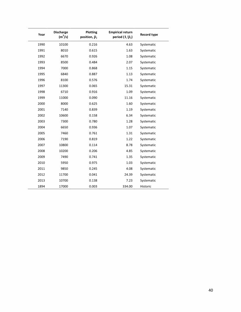
40
Year Discharge
(m3/s)
Plotting
position, �̂�𝒊
Empirical return
period (𝟏/�̂�𝒊) Record type
1990 10100 0.216 4.63 Systematic
1991 8010 0.615 1.63 Systematic
1992 6670 0.926 1.08 Systematic
1993 8500 0.484 2.07 Systematic
1994 7000 0.868 1.15 Systematic
1995 6840 0.887 1.13 Systematic
1996 8100 0.576 1.74 Systematic
1997 11300 0.065 15.31 Systematic
1998 6710 0.916 1.09 Systematic
1999 11000 0.090 11.16 Systematic
2000 8000 0.625 1.60 Systematic
2001 7140 0.839 1.19 Systematic
2002 10600 0.158 6.34 Systematic
2003 7300 0.780 1.28 Systematic
2004 6650 0.936 1.07 Systematic
2005 7460 0.761 1.31 Systematic
2006 7190 0.819 1.22 Systematic
2007 10800 0.114 8.78 Systematic
2008 10200 0.206 4.85 Systematic
2009 7490 0.741 1.35 Systematic
2010 5950 0.975 1.03 Systematic
2011 9850 0.245 4.08 Systematic
2012 11700 0.041 24.39 Systematic
2013 10700 0.138 7.23 Systematic
1894 17000 0.003 334.00 Historic
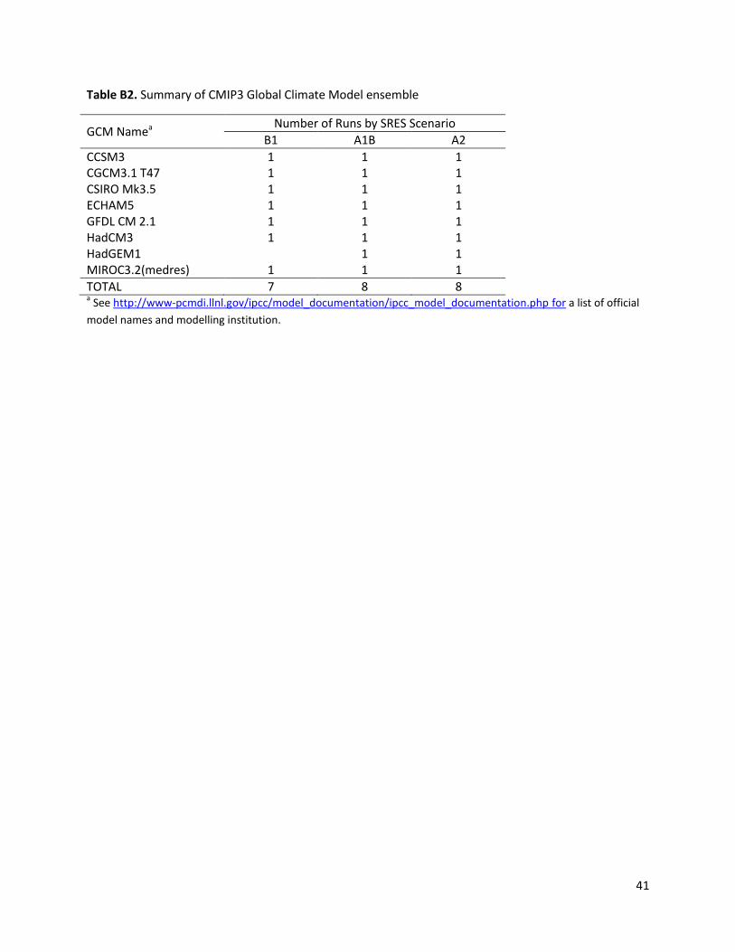
41
Table B2. Summary of CMIP3 Global Climate Model ensemble
GCM Namea Number of Runs by SRES Scenario
B1 A1B A2
CCSM3 1 1 1 CGCM3.1 T47 1 1 1 CSIRO Mk3.5 1 1 1 ECHAM5 1 1 1 GFDL CM 2.1 1 1 1 HadCM3 1 1 1 HadGEM1 1 1 MIROC3.2(medres) 1 1 1
TOTAL 7 8 8 a See http://www-pcmdi.llnl.gov/ipcc/model_documentation/ipcc_model_documentation.php for a list of official
model names and modelling institution.
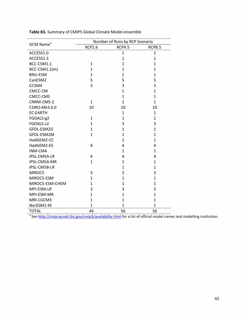
42
Table B3. Summary of CMIP5 Global Climate Model ensemble
GCM Namea Number of Runs by RCP Scenario
RCP2.6 RCP4.5 RCP8.5
ACCESS1.0 1 1 ACCESS1.3 1 1 BCC-CSM1.1 1 1 1 BCC-CSM1.1(m) 1 1 1 BNU-ESM 1 1 1 CanESM2 5 5 5 CCSM4 3 3 3 CMCC-CM 1 1 CMCC-CMS 1 1 CNRM-CM5-2 1 1 1 CSIRO-Mk3.6.0 10 10 10 EC-EARTH 1 1 FGOALS-g2 1 1 1 FGOALS-s2 1 3 3 GFDL-ESM2G 1 1 1 GFDL-ESM2M 1 1 1 HadGEM2-CC 1 1 HadGEM2-ES 4 4 4 INM-CM4 1 1 IPSL-CM5A-LR 4 4 4 IPSL-CM5A-MR 1 1 1 IPSL-CM5B-LR 1 1 MIROC5 3 3 3 MIROC5-ESM 1 1 1 MIROC5-ESM-CHEM 1 1 1 MPI-ESM-LR 3 3 3 MPI-ESM-MR 1 1 1 MRI-CGCM3 1 1 1 NorESM1-M 1 1 1
TOTAL 46 56 56 a See http://cmip-pcmdi.llnl.gov/cmip5/availability.html for a list of official model names and modelling institution.
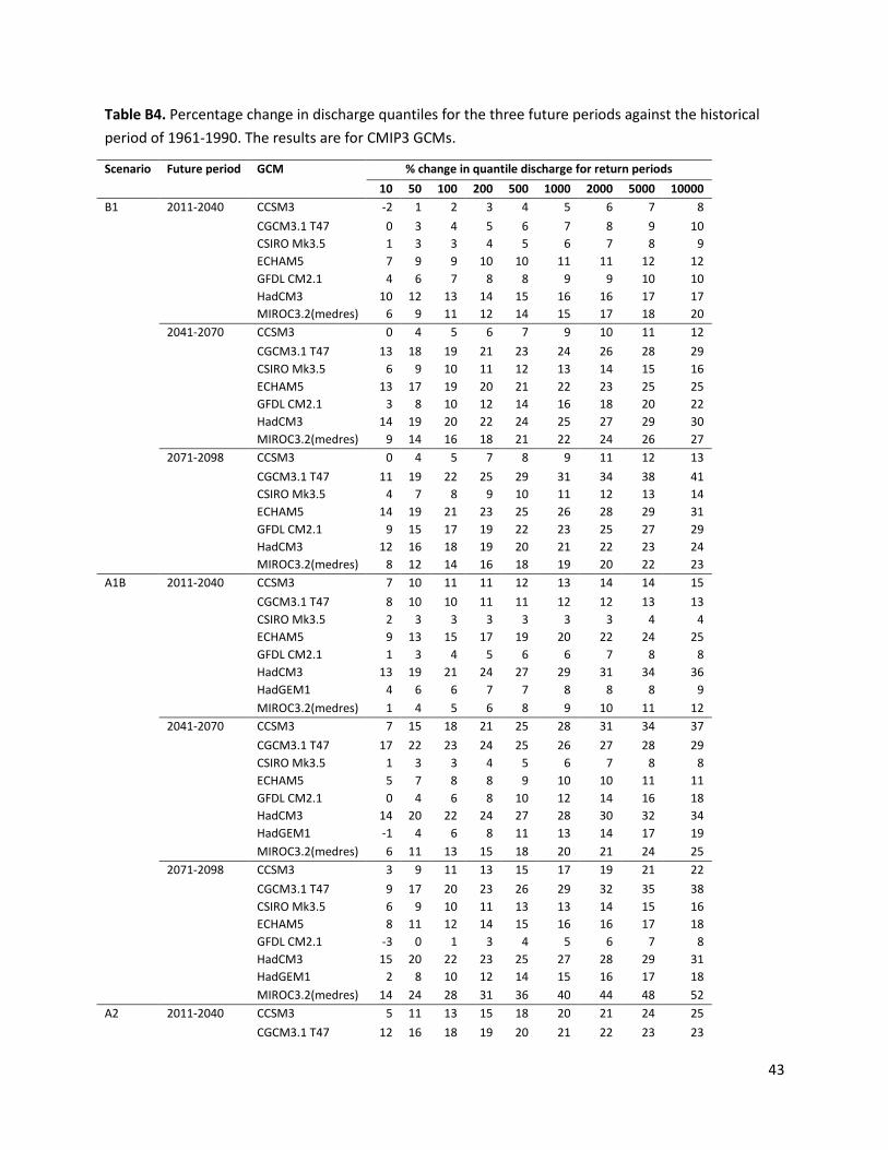
43
Table B4. Percentage change in discharge quantiles for the three future periods against the historical
period of 1961-1990. The results are for CMIP3 GCMs.
Scenario Future period GCM % change in quantile discharge for return periods
10 50 100 200 500 1000 2000 5000 10000
B1 2011-2040 CCSM3 -2 1 2 3 4 5 6 7 8
CGCM3.1 T47 0 3 4 5 6 7 8 9 10
CSIRO Mk3.5 1 3 3 4 5 6 7 8 9
ECHAM5 7 9 9 10 10 11 11 12 12
GFDL CM2.1 4 6 7 8 8 9 9 10 10
HadCM3 10 12 13 14 15 16 16 17 17
MIROC3.2(medres) 6 9 11 12 14 15 17 18 20
2041-2070 CCSM3 0 4 5 6 7 9 10 11 12
CGCM3.1 T47 13 18 19 21 23 24 26 28 29
CSIRO Mk3.5 6 9 10 11 12 13 14 15 16
ECHAM5 13 17 19 20 21 22 23 25 25
GFDL CM2.1 3 8 10 12 14 16 18 20 22
HadCM3 14 19 20 22 24 25 27 29 30
MIROC3.2(medres) 9 14 16 18 21 22 24 26 27
2071-2098 CCSM3 0 4 5 7 8 9 11 12 13
CGCM3.1 T47 11 19 22 25 29 31 34 38 41
CSIRO Mk3.5 4 7 8 9 10 11 12 13 14
ECHAM5 14 19 21 23 25 26 28 29 31
GFDL CM2.1 9 15 17 19 22 23 25 27 29
HadCM3 12 16 18 19 20 21 22 23 24
MIROC3.2(medres) 8 12 14 16 18 19 20 22 23
A1B 2011-2040 CCSM3 7 10 11 11 12 13 14 14 15
CGCM3.1 T47 8 10 10 11 11 12 12 13 13
CSIRO Mk3.5 2 3 3 3 3 3 3 4 4
ECHAM5 9 13 15 17 19 20 22 24 25
GFDL CM2.1 1 3 4 5 6 6 7 8 8
HadCM3 13 19 21 24 27 29 31 34 36
HadGEM1 4 6 6 7 7 8 8 8 9
MIROC3.2(medres) 1 4 5 6 8 9 10 11 12
2041-2070 CCSM3 7 15 18 21 25 28 31 34 37
CGCM3.1 T47 17 22 23 24 25 26 27 28 29
CSIRO Mk3.5 1 3 3 4 5 6 7 8 8
ECHAM5 5 7 8 8 9 10 10 11 11
GFDL CM2.1 0 4 6 8 10 12 14 16 18
HadCM3 14 20 22 24 27 28 30 32 34
HadGEM1 -1 4 6 8 11 13 14 17 19
MIROC3.2(medres) 6 11 13 15 18 20 21 24 25
2071-2098 CCSM3 3 9 11 13 15 17 19 21 22
CGCM3.1 T47 9 17 20 23 26 29 32 35 38
CSIRO Mk3.5 6 9 10 11 13 13 14 15 16
ECHAM5 8 11 12 14 15 16 16 17 18
GFDL CM2.1 -3 0 1 3 4 5 6 7 8
HadCM3 15 20 22 23 25 27 28 29 31
HadGEM1 2 8 10 12 14 15 16 17 18
MIROC3.2(medres) 14 24 28 31 36 40 44 48 52
A2 2011-2040 CCSM3 5 11 13 15 18 20 21 24 25
CGCM3.1 T47 12 16 18 19 20 21 22 23 23
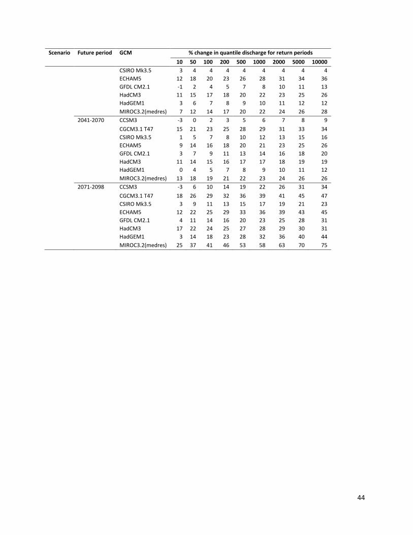
44
Scenario Future period GCM % change in quantile discharge for return periods
10 50 100 200 500 1000 2000 5000 10000
CSIRO Mk3.5 3 4 4 4 4 4 4 4 4
ECHAM5 12 18 20 23 26 28 31 34 36
GFDL CM2.1 -1 2 4 5 7 8 10 11 13
HadCM3 11 15 17 18 20 22 23 25 26
HadGEM1 3 6 7 8 9 10 11 12 12
MIROC3.2(medres) 7 12 14 17 20 22 24 26 28
2041-2070 CCSM3 -3 0 2 3 5 6 7 8 9
CGCM3.1 T47 15 21 23 25 28 29 31 33 34
CSIRO Mk3.5 1 5 7 8 10 12 13 15 16
ECHAM5 9 14 16 18 20 21 23 25 26
GFDL CM2.1 3 7 9 11 13 14 16 18 20
HadCM3 11 14 15 16 17 17 18 19 19
HadGEM1 0 4 5 7 8 9 10 11 12
MIROC3.2(medres) 13 18 19 21 22 23 24 26 26
2071-2098 CCSM3 -3 6 10 14 19 22 26 31 34
CGCM3.1 T47 18 26 29 32 36 39 41 45 47
CSIRO Mk3.5 3 9 11 13 15 17 19 21 23
ECHAM5 12 22 25 29 33 36 39 43 45
GFDL CM2.1 4 11 14 16 20 23 25 28 31
HadCM3 17 22 24 25 27 28 29 30 31
HadGEM1 3 14 18 23 28 32 36 40 44
MIROC3.2(medres) 25 37 41 46 53 58 63 70 75
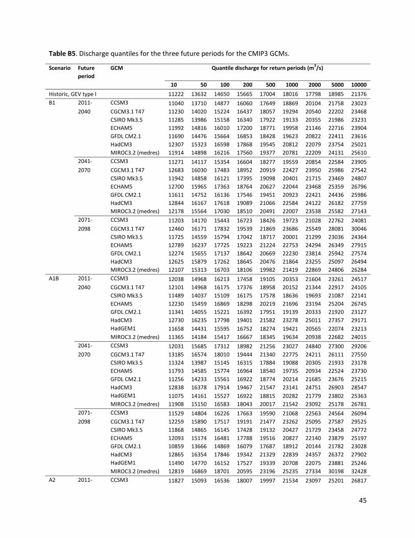
45
Table B5. Discharge quantiles for the three future periods for the CMIP3 GCMs.
Scenario Future
period
GCM Quantile discharge for return periods (m3/s)
10 50 100 200 500 1000 2000 5000 10000
Historic, GEV type I 11222 13632 14650 15665 17004 18016 17798 18985 21376
B1 2011- CCSM3 11040 13710 14877 16060 17649 18869 20104 21758 23023
2040 CGCM3.1 T47 11230 14020 15224 16437 18057 19294 20540 22202 23468
CSIRO Mk3.5 11285 13986 15158 16340 17922 19133 20355 21986 23231
ECHAM5 11992 14816 16010 17200 18771 19958 21146 22716 23904
GFDL CM2.1 11690 14476 15664 16853 18428 19623 20822 22411 23616
HadCM3 12307 15323 16598 17868 19545 20812 22079 23754 25021
MIROC3.2 (medres) 11914 14898 16216 17560 19377 20781 22209 24131 25610
2041- CCSM3 11271 14117 15354 16604 18277 19559 20854 22584 23905
2070 CGCM3.1 T47 12683 16030 17483 18952 20919 22427 23950 25986 27542
CSIRO Mk3.5 11942 14858 16121 17395 19098 20401 21715 23469 24807
ECHAM5 12700 15965 17363 18764 20627 22044 23468 25359 26796
GFDL CM2.1 11611 14752 16136 17546 19451 20923 22421 24436 25986
HadCM3 12844 16167 17618 19089 21066 22584 24122 26182 27759
MIROC3.2 (medres) 12178 15564 17030 18510 20491 22007 23538 25582 27143
2071- CCSM3 11203 14170 15443 16723 18426 19723 21028 22762 24081
2098 CGCM3.1 T47 12460 16171 17832 19539 21869 23686 25549 28081 30046
CSIRO Mk3.5 11725 14559 15794 17042 18717 20001 21299 23036 24364
ECHAM5 12789 16237 17725 19223 21224 22753 24294 26349 27915
GFDL CM2.1 12274 15655 17137 18642 20669 22230 23814 25942 27574
HadCM3 12625 15879 17262 18645 20476 21864 23255 25097 26494
MIROC3.2 (medres) 12107 15313 16703 18106 19982 21419 22869 24806 26284
A1B 2011- CCSM3 12038 14968 16213 17458 19105 20353 21604 23261 24517
2040 CGCM3.1 T47 12101 14968 16175 17376 18958 20152 21344 22917 24105
CSIRO Mk3.5 11489 14037 15109 16175 17578 18636 19693 21087 22141
ECHAM5 12230 15459 16869 18298 20219 21696 23194 25204 26745
GFDL CM2.1 11341 14055 15221 16392 17951 19139 20333 21920 23127
HadCM3 12730 16235 17798 19401 21582 23278 25011 27357 29171
HadGEM1 11658 14431 15595 16752 18274 19421 20565 22074 23213
MIROC3.2 (medres) 11365 14184 15417 16667 18345 19634 20938 22682 24015
2041- CCSM3 12031 15685 17312 18982 21256 23027 24840 27300 29206
2070 CGCM3.1 T47 13185 16574 18010 19444 21340 22775 24211 26111 27550
CSIRO Mk3.5 11324 13987 15145 16315 17884 19088 20305 21933 23178
ECHAM5 11793 14585 15774 16964 18540 19735 20934 22524 23730
GFDL CM2.1 11256 14233 15561 16922 18774 20214 21685 23676 25215
HadCM3 12838 16378 17914 19467 21547 23141 24751 26903 28547
HadGEM1 11075 14161 15527 16922 18815 20282 21779 23802 25363
MIROC3.2 (medres) 11908 15150 16583 18043 20017 21542 23092 25178 26781
2071- CCSM3 11529 14804 16226 17663 19590 21068 22563 24564 26094
2098 CGCM3.1 T47 12259 15890 17517 19191 21477 23262 25095 27587 29525
CSIRO Mk3.5 11868 14865 16145 17428 19132 20427 21729 23458 24772
ECHAM5 12093 15174 16481 17788 19516 20827 22140 23879 25197
GFDL CM2.1 10859 13666 14869 16079 17687 18912 20144 21782 23028
HadCM3 12865 16354 17846 19342 21329 22839 24357 26372 27902
HadGEM1 11490 14770 16152 17527 19339 20708 22075 23881 25246
MIROC3.2 (medres) 12819 16869 18701 20595 23196 25235 27334 30198 32428
A2 2011- CCSM3 11827 15093 16536 18007 19997 21534 23097 25201 26817
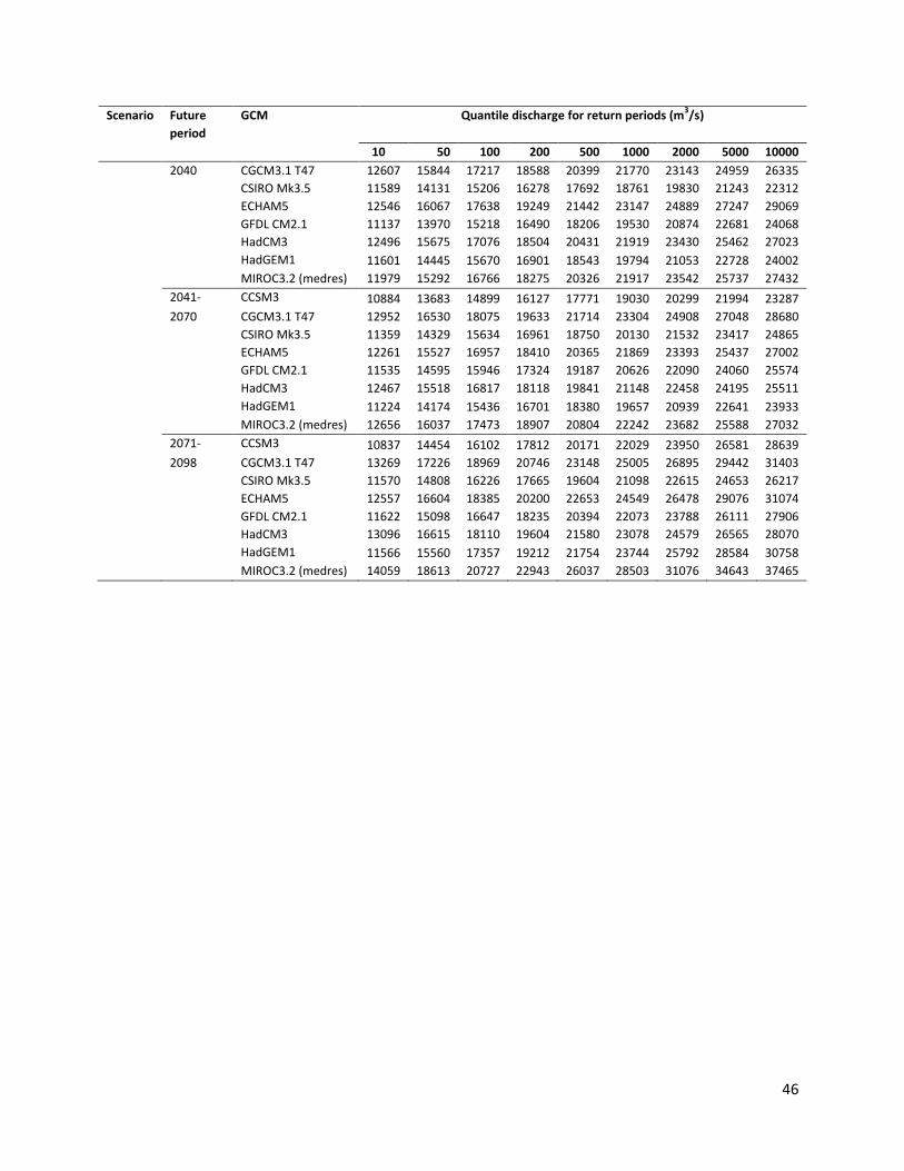
46
Scenario Future
period
GCM Quantile discharge for return periods (m3/s)
10 50 100 200 500 1000 2000 5000 10000
2040 CGCM3.1 T47 12607 15844 17217 18588 20399 21770 23143 24959 26335
CSIRO Mk3.5 11589 14131 15206 16278 17692 18761 19830 21243 22312
ECHAM5 12546 16067 17638 19249 21442 23147 24889 27247 29069
GFDL CM2.1 11137 13970 15218 16490 18206 19530 20874 22681 24068
HadCM3 12496 15675 17076 18504 20431 21919 23430 25462 27023
HadGEM1 11601 14445 15670 16901 18543 19794 21053 22728 24002
MIROC3.2 (medres) 11979 15292 16766 18275 20326 21917 23542 25737 27432
2041- CCSM3 10884 13683 14899 16127 17771 19030 20299 21994 23287
2070 CGCM3.1 T47 12952 16530 18075 19633 21714 23304 24908 27048 28680
CSIRO Mk3.5 11359 14329 15634 16961 18750 20130 21532 23417 24865
ECHAM5 12261 15527 16957 18410 20365 21869 23393 25437 27002
GFDL CM2.1 11535 14595 15946 17324 19187 20626 22090 24060 25574
HadCM3 12467 15518 16817 18118 19841 21148 22458 24195 25511
HadGEM1 11224 14174 15436 16701 18380 19657 20939 22641 23933
MIROC3.2 (medres) 12656 16037 17473 18907 20804 22242 23682 25588 27032
2071- CCSM3 10837 14454 16102 17812 20171 22029 23950 26581 28639
2098 CGCM3.1 T47 13269 17226 18969 20746 23148 25005 26895 29442 31403
CSIRO Mk3.5 11570 14808 16226 17665 19604 21098 22615 24653 26217
ECHAM5 12557 16604 18385 20200 22653 24549 26478 29076 31074
GFDL CM2.1 11622 15098 16647 18235 20394 22073 23788 26111 27906
HadCM3 13096 16615 18110 19604 21580 23078 24579 26565 28070
HadGEM1 11566 15560 17357 19212 21754 23744 25792 28584 30758
MIROC3.2 (medres) 14059 18613 20727 22943 26037 28503 31076 34643 37465
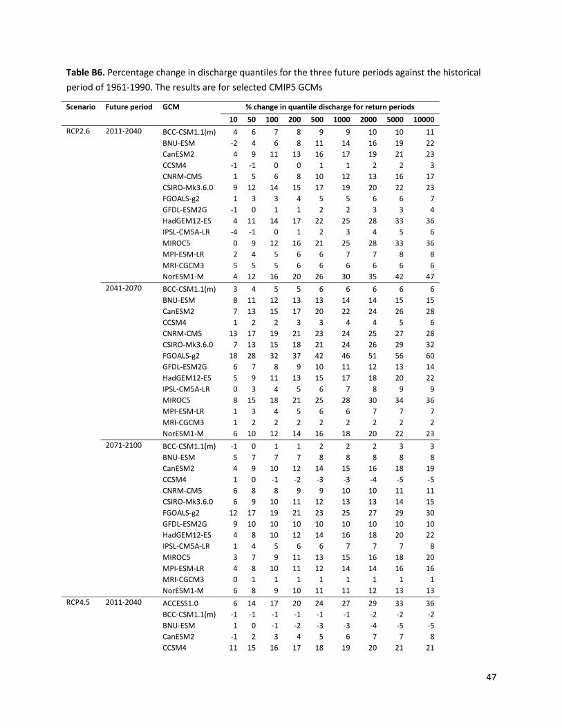
47
Table B6. Percentage change in discharge quantiles for the three future periods against the historical
period of 1961-1990. The results are for selected CMIP5 GCMs
Scenario Future period GCM % change in quantile discharge for return periods
10 50 100 200 500 1000 2000 5000 10000
RCP2.6 2011-2040 BCC-CSM1.1(m) 4 6 7 8 9 9 10 10 11
BNU-ESM -2 4 6 8 11 14 16 19 22
CanESM2 4 9 11 13 16 17 19 21 23
CCSM4 -1 -1 0 0 1 1 2 2 3
CNRM-CM5 1 5 6 8 10 12 13 16 17
CSIRO-Mk3.6.0 9 12 14 15 17 19 20 22 23
FGOALS-g2 1 3 3 4 5 5 6 6 7
GFDL-ESM2G -1 0 1 1 2 2 3 3 4
HadGEM12-ES 4 11 14 17 22 25 28 33 36
IPSL-CM5A-LR -4 -1 0 1 2 3 4 5 6
MIROC5 0 9 12 16 21 25 28 33 36
MPI-ESM-LR 2 4 5 6 6 7 7 8 8
MRI-CGCM3 5 5 5 6 6 6 6 6 6
NorESM1-M 4 12 16 20 26 30 35 42 47
2041-2070 BCC-CSM1.1(m) 3 4 5 5 6 6 6 6 6
BNU-ESM 8 11 12 13 13 14 14 15 15
CanESM2 7 13 15 17 20 22 24 26 28
CCSM4 1 2 2 3 3 4 4 5 6
CNRM-CM5 13 17 19 21 23 24 25 27 28
CSIRO-Mk3.6.0 7 13 15 18 21 24 26 29 32
FGOALS-g2 18 28 32 37 42 46 51 56 60
GFDL-ESM2G 6 7 8 9 10 11 12 13 14
HadGEM12-ES 5 9 11 13 15 17 18 20 22
IPSL-CM5A-LR 0 3 4 5 6 7 8 9 9
MIROC5 8 15 18 21 25 28 30 34 36
MPI-ESM-LR 1 3 4 5 6 6 7 7 7
MRI-CGCM3 1 2 2 2 2 2 2 2 2
NorESM1-M 6 10 12 14 16 18 20 22 23
2071-2100 BCC-CSM1.1(m) -1 0 1 1 2 2 2 3 3
BNU-ESM 5 7 7 7 8 8 8 8 8
CanESM2 4 9 10 12 14 15 16 18 19
CCSM4 1 0 -1 -2 -3 -3 -4 -5 -5
CNRM-CM5 6 8 8 9 9 10 10 11 11
CSIRO-Mk3.6.0 6 9 10 11 12 13 13 14 15
FGOALS-g2 12 17 19 21 23 25 27 29 30
GFDL-ESM2G 9 10 10 10 10 10 10 10 10
HadGEM12-ES 4 8 10 12 14 16 18 20 22
IPSL-CM5A-LR 1 4 5 6 6 7 7 7 8
MIROC5 3 7 9 11 13 15 16 18 20
MPI-ESM-LR 4 8 10 11 12 14 14 16 16
MRI-CGCM3 0 1 1 1 1 1 1 1 1
NorESM1-M 6 8 9 10 11 11 12 13 13
RCP4.5 2011-2040 ACCESS1.0 6 14 17 20 24 27 29 33 36
BCC-CSM1.1(m) -1 -1 -1 -1 -1 -1 -2 -2 -2
BNU-ESM 1 0 -1 -2 -3 -3 -4 -5 -5
CanESM2 -1 2 3 4 5 6 7 7 8
CCSM4 11 15 16 17 18 19 20 21 21
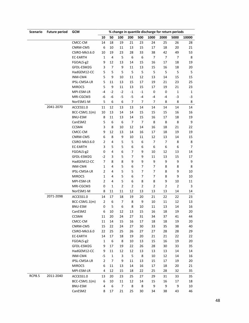
48
Scenario Future period GCM % change in quantile discharge for return periods
10 50 100 200 500 1000 2000 5000 10000
CMCC-CM 14 18 19 21 23 24 25 26 28
CNRM-CM5 6 10 11 13 15 17 18 20 21
CSIRO-Mk3.6.0 10 19 23 28 33 38 42 49 53
EC-EARTH 1 4 5 6 6 7 7 7 8
FGOALS-g2 9 12 13 14 15 16 17 18 19
GFDL-ESM2G 3 7 9 11 13 15 16 18 20
HadGEM12-CC 5 5 5 5 5 5 5 5 5
INM-CM4 5 9 10 11 12 13 14 15 15
IPSL-CM5A-LR 5 11 13 15 17 19 21 23 25
MIROC5 5 9 11 13 15 17 19 21 23
MPI-ESM-LR -4 -2 -2 -1 -1 0 0 1 1
MRI-CGCM3 -6 -6 -5 -5 -4 -4 -4 -3 -3
NorESM1-M 5 6 6 7 7 7 8 8 8
2041-2070 ACCESS1.0 11 12 13 13 14 14 14 14 14
BCC-CSM1.1(m) 10 13 14 14 15 15 15 16 16
BNU-ESM 8 11 13 14 15 16 17 18 19
CanESM2 5 6 6 7 7 8 8 8 9
CCSM4 3 8 10 12 14 16 18 21 22
CMCC-CM 9 12 13 14 16 17 18 19 19
CNRM-CM5 6 8 9 10 11 12 13 14 15
CSIRO-Mk3.6.0 2 4 5 5 6 7 7 8 8
EC-EARTH 3 5 5 6 6 6 6 6 7
FGOALS-g2 0 4 6 7 9 10 12 13 14
GFDL-ESM2G -2 3 5 7 9 11 13 15 17
HadGEM12-CC 7 8 8 9 9 9 9 9 9
INM-CM4 1 4 5 6 7 7 8 8 8
IPSL-CM5A-LR 2 4 5 5 7 7 8 9 10
MIROC5 1 4 5 6 7 7 8 9 10
MPI-ESM-LR 2 4 5 6 8 8 9 10 11
MRI-CGCM3 0 1 2 2 2 2 2 2 3
NorESM1-M 8 11 11 12 13 13 13 14 14
2071-2098 ACCESS1.0 14 17 18 19 20 21 22 22 23
BCC-CSM1.1(m) 2 6 7 8 9 10 11 12 13
BNU-ESM 0 5 6 8 10 11 13 14 16
CanESM2 6 10 12 13 15 16 18 19 20
CCSM4 11 20 24 27 31 34 37 41 44
CMCC-CM 11 14 15 16 17 18 18 19 20
CNRM-CM5 15 22 24 27 30 33 35 38 40
CSIRO-Mk3.6.0 22 25 25 26 27 27 28 28 29
EC-EARTH 14 17 18 19 20 21 21 22 22
FGOALS-g2 1 6 8 10 13 15 16 19 20
GFDL-ESM2G 9 17 19 22 26 28 30 33 35
HadGEM12-CC 9 11 12 12 13 13 13 14 14
INM-CM4 -5 1 3 5 8 10 12 14 16
IPSL-CM5A-LR 2 7 9 11 13 15 17 19 20
MIROC5 6 11 13 14 16 17 18 20 21
MPI-ESM-LR 4 12 15 18 22 25 28 32 35
RCP8.5 2011-2040 ACCESS1.0 13 20 23 25 27 29 31 33 35
BCC-CSM1.1(m) 6 10 11 12 14 15 16 17 18
BNU-ESM 4 6 7 8 8 9 9 9 10
CanESM2 8 17 21 25 30 34 38 43 46
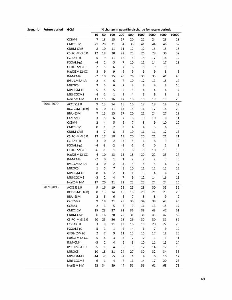
49
Scenario Future period GCM % change in quantile discharge for return periods
10 50 100 200 500 1000 2000 5000 10000
CCSM4 7 13 15 17 20 22 24 26 28
CMCC-CM 21 28 31 34 38 41 44 48 52
CNRM-CM5 8 10 11 11 12 12 13 13 13
CSIRO-Mk3.6.0 12 18 20 22 25 26 28 30 32
EC-EARTH 5 9 11 12 14 15 17 18 19
FGOALS-g2 -4 2 5 7 10 12 14 17 19
GFDL-ESM2G 2 5 6 7 8 8 9 9 9
HadGEM12-CC 8 9 9 9 9 9 9 8 8
INM-CM4 -2 10 15 20 26 30 35 41 46
IPSL-CM5A-LR -2 4 6 7 10 12 13 15 17
MIROC5 3 5 6 7 8 8 9 9 10
MPI-ESM-LR -5 -5 -5 -5 -5 -4 -4 -4 -4
MRI-CGCM3 -4 -1 1 2 4 5 6 8 9
NorESM1-M 13 15 16 17 18 18 19 19 20
2041-2070 ACCESS1.0 9 13 14 15 16 17 18 18 19
BCC-CSM1.1(m) 6 10 11 13 14 16 17 18 20
BNU-ESM 7 13 15 17 20 22 24 27 29
CanESM2 3 5 6 7 8 9 10 10 11
CCSM4 2 4 5 6 7 8 9 10 10
CMCC-CM 0 1 2 3 4 4 5 6 6
CNRM-CM5 4 7 8 8 10 11 11 12 13
CSIRO-Mk3.6.0 13 17 18 19 20 20 21 21 21
EC-EARTH -3 0 2 3 5 6 8 9 10
FGOALS-g2 -4 -3 -2 -2 -1 -1 0 1 1
GFDL-ESM2G -6 -1 1 3 6 8 10 13 15
HadGEM12-CC 4 10 13 15 18 20 22 25 27
INM-CM4 -2 0 1 1 2 2 2 3 3
IPSL-CM5A-LR -3 0 2 3 4 5 5 6 7
MIROC5 1 5 7 8 10 11 11 13 13
MPI-ESM-LR -8 -4 -2 -1 1 3 4 6 7
MRI-CGCM3 -3 2 4 7 9 12 14 16 18
NorESM1-M 17 20 21 22 23 23 24 24 25
2071-2098 ACCESS1.0 9 16 19 22 25 28 30 33 35
BCC-CSM1.1(m) 8 13 14 16 18 20 21 23 25
BNU-ESM 2 5 6 6 7 8 8 9 9
CanESM2 9 18 21 25 30 34 38 43 46
CCSM4 -2 3 5 7 9 11 13 15 17
CMCC-CM 15 23 27 31 36 39 43 47 51
CNRM-CM5 6 16 20 25 31 36 41 47 52
CSIRO-Mk3.6.0 20 25 26 28 29 30 30 31 32
EC-EARTH 3 9 11 13 16 18 20 22 23
FGOALS-g2 -5 -1 1 2 4 6 7 9 10
GFDL-ESM2G 2 7 9 11 13 15 17 18 20
HadGEM12-CC -5 -4 -3 -3 -2 -2 -1 -1 -1
INM-CM4 -5 2 4 6 8 10 11 13 14
IPSL-CM5A-LR -5 1 4 6 9 12 14 17 19
MIROC5 10 18 21 24 27 30 32 34 36
MPI-ESM-LR -14 -7 -5 -2 1 4 6 10 12
MRI-CGCM3 -6 1 4 7 11 14 17 20 23
NorESM1-M 22 34 39 44 51 56 61 68 73

50
Table B7. Discharge quantiles for the three future periods for the selected CMIP5 GCMs.
Scenario Future period
GCM Quantile Discharge for return periods (m3/s)
10 50 100 200 500 1000 2000 5000 10000
Historic, GEV type I 11222 13632 14650 15665 17004 18016 17798 18985 21376
RCP2.6 2011- BCC-CSM1.1(m) 11630 14473 15677 16879 18468 19672 20876 22470 23677
2040 BNU-ESM 11041 14114 15504 16942 18918 20470 22071 24261 25972
CanESM2 11698 14909 16314 17741 19661 21140 22639 24652 26196
CCSM4 11071 13558 14631 15710 17150 18250 19358 20835 21961
CNRM-CM5 11378 14267 15563 16895 18710 20123 21569 23528 25043
CSIRO-Mk3.6.0 12213 15321 16685 18071 19938 21376 22836 24795 26299
FGOALS-g2 11345 14018 15161 16306 17827 18983 20142 21680 22846
GFDL-ESM2G 11108 13650 14741 15837 17295 18406 19524 21011 22144
HadGEM12-ES 11663 15129 16724 18388 20692 22513 24399 26990 29020
IPSL-CM5A-LR 10761 13480 14650 15828 17397 18593 19798 21401 22621
MIROC5 11231 14827 16473 18188 20562 22440 24387 27068 29173
MPI-ESM-LR 11404 14195 15371 16542 18085 19251 20416 21955 23118
MRI-CGCM3 11789 14361 15452 16540 17977 19065 20154 21594 22685
NorESM1-M 11624 15217 16932 18761 21364 23478 25723 28895 31455
2041- BCC-CSM1.1(m) 11546 14245 15374 16493 17962 19068 20169 21619 22713 2070 BNU-ESM 12104 15127 16387 17635 19270 20498 21720 23328 24539 CanESM2 11958 15372 16862 18372 20402 21964 23547 25669 27296 CCSM4 11334 13896 15000 16112 17595 18728 19870 21393 22554 CNRM-CM5 12709 16013 17447 18895 20833 22316 23813 25812 27337 CSIRO-Mk3.6.0 12023 15381 16896 18460 20604 22283 24011 26367 28201 FGOALS-g2 13274 17483 19410 21414 24185 26373 28639 31750 34189 GFDL-ESM2G 11885 14643 15849 17073 18719 19986 21271 22996 24321 HadGEM12-ES 11751 14857 16231 17634 19529 20994 22482 24482 26017 IPSL-CM5A-LR 11223 14025 15228 16436 18044 19268 20499 22135 23379 MIROC5 12148 15744 17349 18996 21241 22989 24779 27205 29084 MPI-ESM-LR 11300 14098 15273 16441 17977 19135 20290 21815 22966 MRI-CGCM3 11326 13855 14912 15959 17331 18363 19391 20743 21762 NorESM1-M 11852 15044 16446 17873 19796 21281 22789 24817 26377
2071- BCC-CSM1.1(m) 11075 13679 14775 15864 17298 18380 19460 20885 21961 2098 BNU-ESM 11804 14566 15707 16831 18298 19396 20485 21914 22987 CanESM2 11692 14790 16134 17493 19311 20705 22113 23995 25432 CCSM4 11327 13579 14498 15397 16562 17429 18284 19400 20236 CNRM-CM5 11915 14693 15872 17048 18602 19779 20957 22515 23695 CSIRO-Mk3.6.0 11903 14862 16119 17375 19037 20297 21558 23229 24495 FGOALS-g2 12590 15970 17451 18956 20982 22540 24120 26238 27861 GFDL-ESM2G 12236 14975 16122 17259 18750 19872 20990 22461 23570 HadGEM12-ES 11635 14739 16118 17527 19437 20914 22418 24444 26001 IPSL-CM5A-LR 11380 14208 15387 16554 18084 19234 20378 21884 23018 MIROC5 11504 14647 16017 17406 19271 20704 22155 24099 25587 MPI-ESM-LR 11721 14774 16080 17389 19129 20453 21784 23552 24897 MRI-CGCM3 11208 13714 14766 15811 17185 18220 19252 20614 21641 NorESM1-M 11884 14763 15990 17217 18844 20079 21318 22961 24207
RCP4.5 2011- ACCESS1.0 11395 13855 14892 15924 17285 18311 19337 20691 21715 2040 BCC-CSM1.1(m) 11779 14559 15757 16962 18570 19797 21033 22680 23935 BNU-ESM 11571 14712 16062 17419 19228 20608 21998 23850 25262 CanESM2 11457 14139 15272 16402 17893 19020 20147 21637 22764 CCSM4 10389 12510 13416 14322 15524 16436 17351 18564 19485
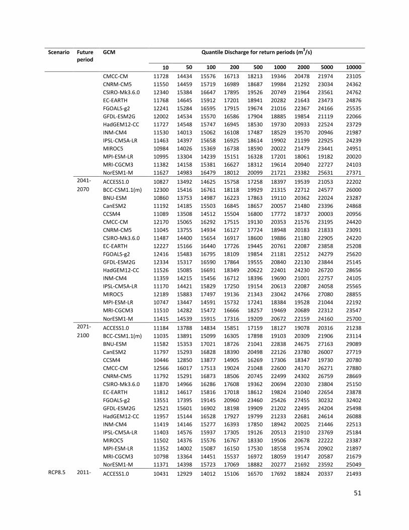
51
Scenario Future period
GCM Quantile Discharge for return periods (m3/s)
10 50 100 200 500 1000 2000 5000 10000
CMCC-CM 11728 14434 15576 16713 18213 19346 20478 21974 23105 CNRM-CM5 11550 14459 15719 16989 18687 19984 21292 23034 24362 CSIRO-Mk3.6.0 12340 15384 16647 17895 19526 20749 21964 23561 24762 EC-EARTH 11768 14645 15912 17201 18941 20282 21643 23473 24876 FGOALS-g2 12241 15284 16595 17915 19674 21016 22367 24166 25535 GFDL-ESM2G 12002 14534 15570 16586 17904 18885 19854 21119 22066 HadGEM12-CC 11727 14548 15747 16945 18530 19730 20933 22524 23729 INM-CM4 11530 14013 15062 16108 17487 18529 19570 20946 21987 IPSL-CM5A-LR 11463 14397 15658 16925 18614 19902 21199 22925 24239 MIROC5 10984 14026 15369 16738 18590 20022 21479 23441 24951 MPI-ESM-LR 10995 13304 14239 15151 16328 17201 18061 19182 20020 MRI-CGCM3 11382 14158 15381 16627 18312 19614 20940 22727 24103 NorESM1-M 11627 14983 16479 18012 20099 21721 23382 25631 27371
2041- ACCESS1.0 10827 13492 14625 15758 17258 18397 19539 21053 22202 2070 BCC-CSM1.1(m) 12300 15416 16761 18118 19929 21315 22712 24577 26000 BNU-ESM 10860 13753 14987 16223 17863 19110 20362 22024 23287 CanESM2 11192 14185 15503 16845 18657 20057 21480 23396 24868 CCSM4 11089 13508 14512 15504 16800 17772 18737 20003 20956 CMCC-CM 12170 15065 16292 17515 19130 20353 21576 23195 24420 CNRM-CM5 11045 13755 14934 16127 17724 18948 20183 21833 23091 CSIRO-Mk3.6.0 11487 14400 15654 16917 18600 19886 21180 22905 24220 EC-EARTH 12227 15166 16440 17726 19445 20761 22087 23858 25208 FGOALS-g2 12416 15483 16795 18109 19854 21181 22512 24279 25620 GFDL-ESM2G 12334 15317 16590 17864 19555 20840 22130 23844 25145 HadGEM12-CC 11526 15085 16691 18349 20622 22401 24230 26720 28656 INM-CM4 11359 14215 15456 16712 18396 19690 21001 22757 24105 IPSL-CM5A-LR 11170 14421 15829 17250 19154 20613 22087 24058 25565 MIROC5 12189 15883 17497 19136 21343 23042 24766 27080 28855 MPI-ESM-LR 10747 13447 14591 15732 17241 18384 19528 21044 22192 MRI-CGCM3 11510 14282 15472 16666 18257 19469 20689 22312 23547 NorESM1-M 11415 14539 15915 17316 19209 20672 22159 24160 25700
2071- ACCESS1.0 11184 13788 14834 15851 17159 18127 19078 20316 21238 2100 BCC-CSM1.1(m) 11035 13891 15099 16305 17898 19103 20309 21906 23114 BNU-ESM 11582 15353 17021 18726 21041 22838 24675 27163 29089 CanESM2 11797 15293 16828 18390 20498 22126 23780 26007 27719 CCSM4 10446 12850 13877 14905 16269 17306 18347 19730 20780 CMCC-CM 12566 16017 17513 19024 21048 22600 24170 26271 27880 CNRM-CM5 11792 15291 16873 18506 20745 22499 24302 26759 28669 CSIRO-Mk3.6.0 11870 14966 16286 17608 19362 20694 22030 23804 25150 EC-EARTH 11812 14617 15816 17018 18612 19824 21040 22654 23878 FGOALS-g2 13551 17395 19145 20960 23460 25426 27455 30232 32402 GFDL-ESM2G 12521 15601 16902 18198 19909 21202 22495 24204 25498 HadGEM12-CC 11957 15144 16528 17927 19799 21233 22681 24614 26088 INM-CM4 11419 14146 15277 16393 17850 18942 20025 21446 22513 IPSL-CM5A-LR 11403 14576 15937 17305 19126 20513 21910 23769 25184 MIROC5 11502 14376 15576 16767 18330 19506 20678 22222 23387 MPI-ESM-LR 11352 14002 15087 16150 17530 18558 19574 20902 21897 MRI-CGCM3 10798 13364 14451 15537 16972 18059 19147 20587 21679 NorESM1-M 11371 14398 15723 17069 18882 20277 21692 23592 25049
RCP8.5 2011- ACCESS1.0 10431 12929 14012 15106 16570 17692 18824 20337 21493
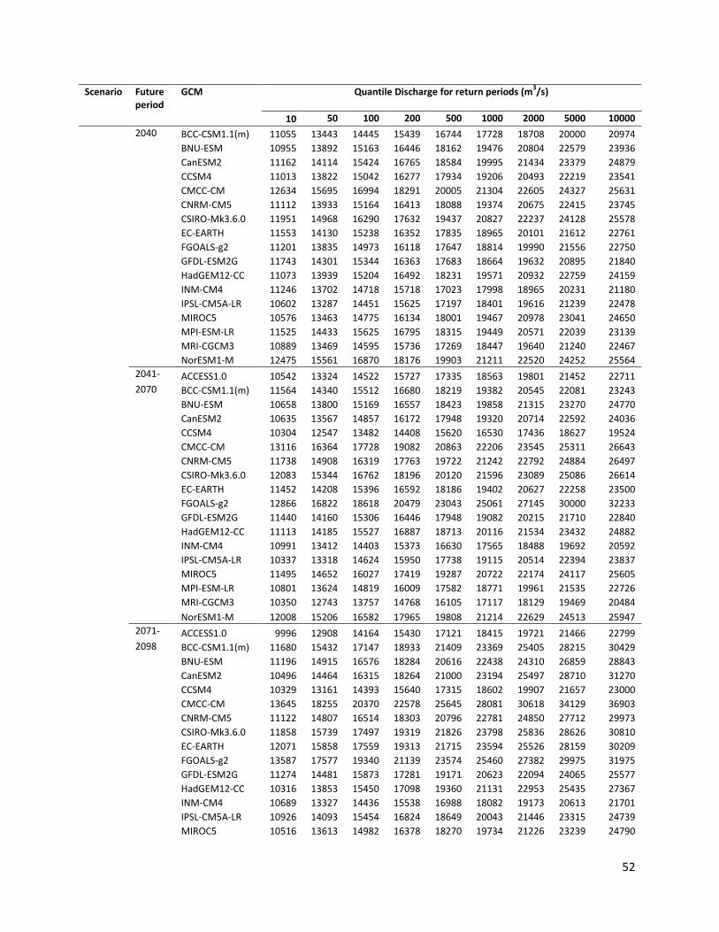
52
Scenario Future period
GCM Quantile Discharge for return periods (m3/s)
10 50 100 200 500 1000 2000 5000 10000
2040 BCC-CSM1.1(m) 11055 13443 14445 15439 16744 17728 18708 20000 20974 BNU-ESM 10955 13892 15163 16446 18162 19476 20804 22579 23936 CanESM2 11162 14114 15424 16765 18584 19995 21434 23379 24879 CCSM4 11013 13822 15042 16277 17934 19206 20493 22219 23541 CMCC-CM 12634 15695 16994 18291 20005 21304 22605 24327 25631 CNRM-CM5 11112 13933 15164 16413 18088 19374 20675 22415 23745 CSIRO-Mk3.6.0 11951 14968 16290 17632 19437 20827 22237 24128 25578 EC-EARTH 11553 14130 15238 16352 17835 18965 20101 21612 22761 FGOALS-g2 11201 13835 14973 16118 17647 18814 19990 21556 22750 GFDL-ESM2G 11743 14301 15344 16363 17683 18664 19632 20895 21840 HadGEM12-CC 11073 13939 15204 16492 18231 19571 20932 22759 24159 INM-CM4 11246 13702 14718 15718 17023 17998 18965 20231 21180 IPSL-CM5A-LR 10602 13287 14451 15625 17197 18401 19616 21239 22478 MIROC5 10576 13463 14775 16134 18001 19467 20978 23041 24650 MPI-ESM-LR 11525 14433 15625 16795 18315 19449 20571 22039 23139 MRI-CGCM3 10889 13469 14595 15736 17269 18447 19640 21240 22467 NorESM1-M 12475 15561 16870 18176 19903 21211 22520 24252 25564
2041- ACCESS1.0 10542 13324 14522 15727 17335 18563 19801 21452 22711 2070 BCC-CSM1.1(m) 11564 14340 15512 16680 18219 19382 20545 22081 23243 BNU-ESM 10658 13800 15169 16557 18423 19858 21315 23270 24770 CanESM2 10635 13567 14857 16172 17948 19320 20714 22592 24036 CCSM4 10304 12547 13482 14408 15620 16530 17436 18627 19524 CMCC-CM 13116 16364 17728 19082 20863 22206 23545 25311 26643 CNRM-CM5 11738 14908 16319 17763 19722 21242 22792 24884 26497 CSIRO-Mk3.6.0 12083 15344 16762 18196 20120 21596 23089 25086 26614 EC-EARTH 11452 14208 15396 16592 18186 19402 20627 22258 23500 FGOALS-g2 12866 16822 18618 20479 23043 25061 27145 30000 32233 GFDL-ESM2G 11440 14160 15306 16446 17948 19082 20215 21710 22840 HadGEM12-CC 11113 14185 15527 16887 18713 20116 21534 23432 24882 INM-CM4 10991 13412 14403 15373 16630 17565 18488 19692 20592 IPSL-CM5A-LR 10337 13318 14624 15950 17738 19115 20514 22394 23837 MIROC5 11495 14652 16027 17419 19287 20722 22174 24117 25605 MPI-ESM-LR 10801 13624 14819 16009 17582 18771 19961 21535 22726 MRI-CGCM3 10350 12743 13757 14768 16105 17117 18129 19469 20484 NorESM1-M 12008 15206 16582 17965 19808 21214 22629 24513 25947
2071- ACCESS1.0 9996 12908 14164 15430 17121 18415 19721 21466 22799 2098 BCC-CSM1.1(m) 11680 15432 17147 18933 21409 23369 25405 28215 30429 BNU-ESM 11196 14915 16576 18284 20616 22438 24310 26859 28843 CanESM2 10496 14464 16315 18264 21000 23194 25497 28710 31270 CCSM4 10329 13161 14393 15640 17315 18602 19907 21657 23000 CMCC-CM 13645 18255 20370 22578 25645 28081 30618 34129 36903 CNRM-CM5 11122 14807 16514 18303 20796 22781 24850 27712 29973 CSIRO-Mk3.6.0 11858 15739 17497 19319 21826 23798 25836 28626 30810 EC-EARTH 12071 15858 17559 19313 21715 23594 25526 28159 30209 FGOALS-g2 13587 17577 19340 21139 23574 25460 27382 29975 31975 GFDL-ESM2G 11274 14481 15873 17281 19171 20623 22094 24065 25577 HadGEM12-CC 10316 13853 15450 17098 19360 21131 22953 25435 27367 INM-CM4 10689 13327 14436 15538 16988 18082 19173 20613 21701 IPSL-CM5A-LR 10926 14093 15454 16824 18649 20043 21446 23315 24739 MIROC5 10516 13613 14982 16378 18270 19734 21226 23239 24790
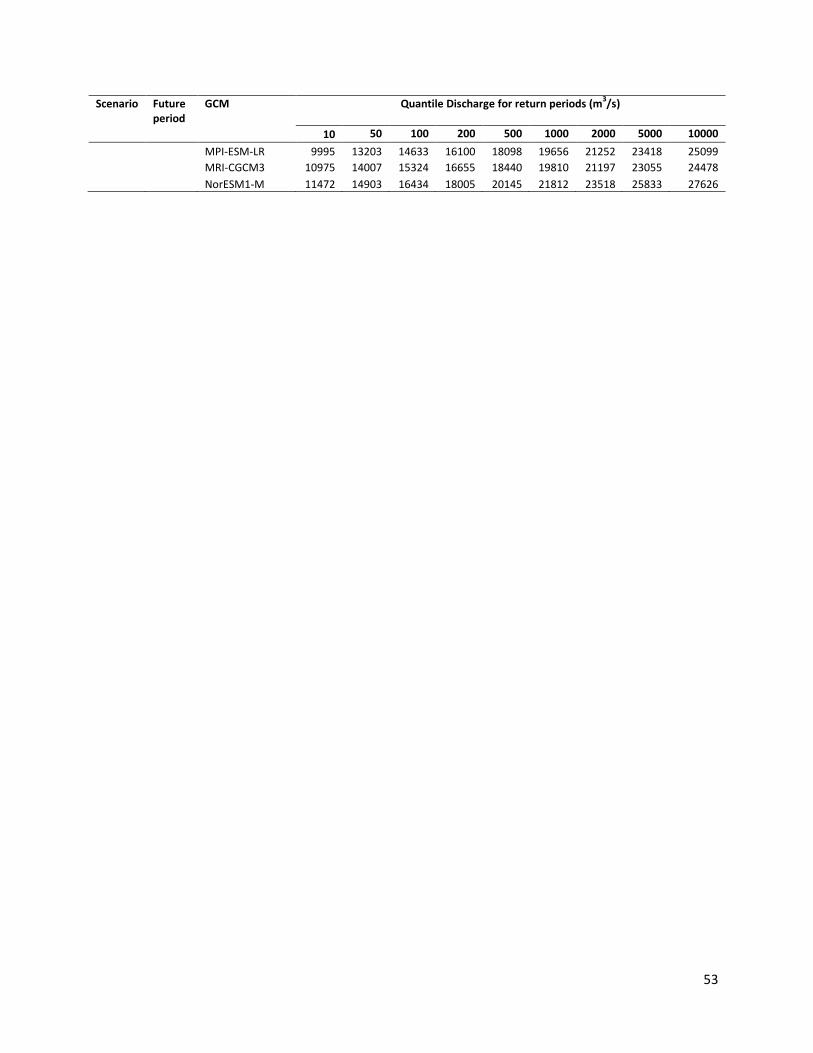
53
Scenario Future period
GCM Quantile Discharge for return periods (m3/s)
10 50 100 200 500 1000 2000 5000 10000
MPI-ESM-LR 9995 13203 14633 16100 18098 19656 21252 23418 25099 MRI-CGCM3 10975 14007 15324 16655 18440 19810 21197 23055 24478 NorESM1-M 11472 14903 16434 18005 20145 21812 23518 25833 27626
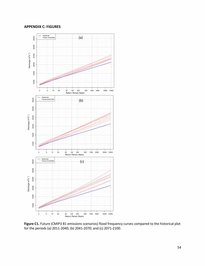
54
APPENDIX C: FIGURES
Figure C1. Future (CMIP3 B1 emissions scenarios) flood frequency curves compared to the historical plot for the periods (a) 2011-2040; (b) 2041-2070; and (c) 2071-2100.
(a)
(b)
(c)
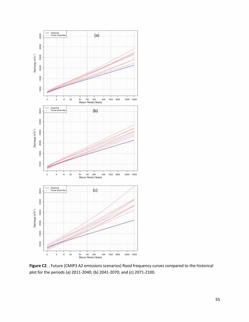
55
Figure C2. . Future (CMIP3 A2 emissions scenarios) flood frequency curves compared to the historical
plot for the periods (a) 2011-2040; (b) 2041-2070; and (c) 2071-2100.
(a)
(b)
(c)
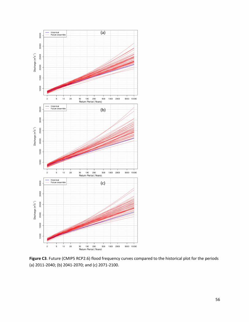
56
Figure C3. Future (CMIP5 RCP2.6) flood frequency curves compared to the historical plot for the periods
(a) 2011-2040; (b) 2041-2070; and (c) 2071-2100.
(a)
(b)
(c)
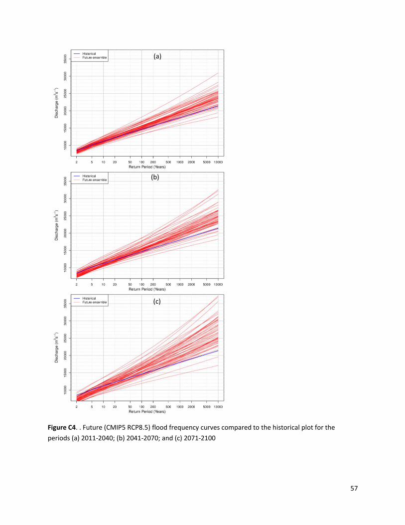
57
Figure C4. . Future (CMIP5 RCP8.5) flood frequency curves compared to the historical plot for the
periods (a) 2011-2040; (b) 2041-2070; and (c) 2071-2100
(a)
(b)
(c)


![Agency Coordination: Fraser River Estuary Management Program [FREMP] 1985-2003](https://static.cupdf.com/doc/110x72/568151bc550346895dbfed17/agency-coordination-fraser-river-estuary-management-program-fremp-1985-2003-56a33ab2af530.jpg)