Sensorless Drives for
Aerospace Applications
Stephen Borman
Thesis Submitted for the degree of
Engineering Doctorate – Power Electronics,
Machines and Drives
School of Electrical,
Electronic and Computer
Engineering
University of Newcastle upon Tyne
April 2012

i
Abstract
This Engineering Doctorate thesis investigates the different implementations and
theories allowing drives to control motors using sensorless techniques that could be
used in an aerospace environment. A range of converter topologies and their control
will be examined to evaluate the possible techniques that will allow a robust and
reliable drive algorithm to be implemented. The focus of the research is around
sensorless drives for fuel pump applications, with the potential to replace an existing
analogue implementation that is embedded in a fuel pump, contained within the fuel
tank. The motor choice (Brushless DC) reflects the requirement for endurance and tight
speed control over the life of the aircraft.
The study of currently understood sensorless control will allow a critical analysis over
the best and most robust sensorless control technique for a controller of this nature,
where reliability is a fundamental requirement.
Eaton Aerospace, Titchfield have sponsored this Engineering Doctorate to further their
understanding of the technologies and methodologies that will allow future motor drives
produced to keep a competitive edge.

ii
Acknowledgements
My thanks have to be made to Keith Evernden who initially led the programme from
Eaton, Titchfield, and Dr Dave Atkinson and Prof. Alan Jack from the University of
Newcastle-upon-Tyne for their academic input throughout the course of this
Engineering Doctorate. Thanks must also be made to Mick Lovell and Terry Wood
who have been part of the succession of managers under whom this project has fallen at
Eaton, and to Brian Pollard (Principal Engineer, Eaton) for his technical input during
my research at the Eaton facility.
My wife, Nicola, has shown unerring support during the write up of this thesis, and
motivation to bring the project to a successful conclusion. I cannot thank her enough.

iii
Section .................................................................................................................... Page
Abstract ......................................................................................................................... i
Acknowledgements ...................................................................................................... ii
Chapter 1. Introduction ............................................................................................ 1
1.1 Background to the project .................................................................................. 1
1.1.1 Transformer Rectifier Unit (TRU) .............................................................. 3
1.1.2 Current Source ............................................................................................ 4
1.1.3 Auxiliary power supply and fault detection ................................................ 6
1.1.4 Motor Drive ................................................................................................. 7
1.1.5 Rationale for Implementation using a Current Source ................................ 8
Chapter 2. Sensorless Control Schemes ................................................................ 10
2.1 Rotor Position Requirements ............................................................................ 10
2.2 Rotor Position Determination ........................................................................... 11
2.2.1 Inductance Variation ................................................................................. 11
2.2.2 High Frequency Injection .......................................................................... 13
2.2.3 Flux Linkage Estimation ........................................................................... 14
2.2.4 Position Estimation using an Observer ..................................................... 18
2.2.5 BEMF zero crossing detection .................................................................. 19
2.3 Justification for choosing BEMF detection ...................................................... 22
2.4 Sensorless Control for Different Motor Types ................................................. 23
2.5 Alternative Converter Topologies .................................................................... 24
2.5.1 Matrix Converters ..................................................................................... 24
2.5.2 Reduced Matrix Converter ........................................................................ 26
2.5.3 Multi – stage power converter topologies ................................................. 26
iv
2.5.4 Analysis of Converter Technologies ......................................................... 28
2.6 Simulation ........................................................................................................ 30
2.7 Summary .......................................................................................................... 32
Chapter 3. Converter Implementation .................................................................. 33
3.1 Controller to be used for research .................................................................... 33
3.2 Single Event Upsets .......................................................................................... 34
3.2.1 Single Event Upset – Single Point ............................................................ 35
3.2.2 Multi Gate Upset ....................................................................................... 35
3.2.3 Gate Rupture ............................................................................................. 35
3.2.4 SEU Mitigation Techniques ...................................................................... 36
3.3 Phase Locked Loops ......................................................................................... 37
3.4 ML4425 PLL .................................................................................................... 37
3.4.1 4046 Edge Triggered PLL ......................................................................... 41
3.5 DSP Implementation (ML4425 PLL) ............................................................... 48
3.6 DSP Implementation (4046 Edge Triggered PLL) ........................................... 49
3.7 4046 DSP Implementation with Analogue Filter ............................................. 53
3.8 Possible Start up Problems ............................................................................... 54
3.9 Digitally matching the analogue filter response ............................................... 57
3.10 Motor Characteristics .................................................................................... 58
3.11 Motor characteristics..................................................................................... 59
3.12 Software Structure for DSP Sensorless BEMF detection ............................. 60
3.13 Commutation Software Structure ................................................................. 62
3.13.1 Align .......................................................................................................... 62
3.13.2 Ramp ......................................................................................................... 64
3.13.3 Run ............................................................................................................ 64

v
3.14 Commutation Strategy .................................................................................. 65
3.15 Two phase equivalent ................................................................................... 71
3.16 Take Back Half (TBH) Control .................................................................... 74
3.17 Take Back All ............................................................................................... 85
3.17.1 Stability Requirement................................................................................ 85
3.17.2 Phase Error ................................................................................................ 93
3.18 DSP Hardware Voltage Measurement .......................................................... 94
3.19 Current measurement .................................................................................... 98
3.20 Summary ....................................................................................................... 99
Chapter 4. Experimental Results from Sensorless BLDC drive ....................... 101
4.1 Qualification of Hardware for flight .............................................................. 107
4.2 Pump Operation .............................................................................................. 109
Chapter 5. Sine Wave Induction Motor Drive.................................................... 112
5.1 Requirement for Induction Motor Drive ........................................................ 112
5.2 Concept Demonstrator .................................................................................... 112
Chapter 6. Conclusions and Further Work ........................................................ 121
6.1 Conclusions .................................................................................................... 121
6.2 Further Work .................................................................................................. 123
References ................................................................................................................. 125
Abbreviations and symbols used ............................................................................ 136
Appendix A. Motor Details .................................................................................. 137
Appendix B. IGBT Gate Drive Circuit ............................................................... 148
Appendix C. Flow Charts for Sinewave Induction Motor Drive ...................... 150
Appendix D. Circuit Diagrams ............................................................................ 156
Appendix E. Saber Simulation ............................................................................ 158

vi
Appendix F. PSim Simulations ............................................................................ 161
Appendix G. HEF4046 PLL Datasheet ............................................................... 164

vii
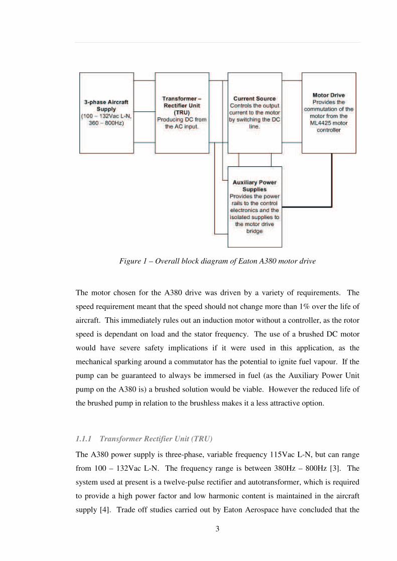
Figure 1 – Overall block diagram of Eaton A380 motor drive ......................................... 3
Figure 2 - TRU showing Autotransformer and rectifier ................................................... 4
Figure 3 - Current Source Circuit diagram ....................................................................... 5
Figure 4 - Motor drive bridge............................................................................................ 7
Figure 5 – Permanent-magnet salient rotor machine flux linkages and incremental
inductance as a function of rotor position ....................................................................... 12
Figure 6 - Closed loop estimator using mechanical model ............................................. 16
Figure 7 - Closed loop observer without mechanical model .......................................... 18
Figure 8 - Observer method for position estimation ....................................................... 19
Figure 9 - Three phase currents in a BLDC .................................................................... 20
Figure 10 – Saw-tooth waveform from three-phase BEMF signals on the ML4425...... 20
Figure 11 - Virtual star point creation ............................................................................. 21
Figure 12 - Full matrix converter .................................................................................... 25
Figure 13 - 12 switch matrix converter topology ............................................................ 26
Figure 14 - Two-stage converter ..................................................................................... 27
Figure 15 - Results from BLDC ...................................................................................... 31
Figure 16 – TMS320F2812 development kit (image from development kit datasheet) . 33
Figure 17 – Neutron Flux wrt altitude............................................................................. 34
Figure 18 - Gated off period ........................................................................................... 38
Figure 19 - Voltage variation with phase ........................................................................ 39
Figure 20 - Phase comparator 1 in 4046 waveforms....................................................... 40
Figure 21 - Diagram of ML4425 PLL arrangement [5][82] ........................................... 40
Figure 22 - Transfer functions of ML4425 PLL [5][82] ................................................. 41
Figure 23 - 4046 functional block diagram taken from data sheet ................................. 42
Figure 24 - Typical waveforms for 4046 PLL in edge triggered mode .......................... 42
viii
Figure 25 – Phase error generated by 4046 edge triggered PLL..................................... 43
Figure 26 - Mechanical model of motor ......................................................................... 45
Figure 27 – Acceleration results from step input to Simulink model ............................. 46
Figure 28 - Initial acceleration from step input to Simulink model ................................ 46
Figure 29 - Align currents through motor and bridge ..................................................... 49
Figure 30 – 4046 edge triggered PLL frequency from ideal BEMF zero crossing......... 50
Figure 31 - Frequency updates from three BEMF signals .............................................. 51
Figure 32 - DSP implementation of 4046 edge triggered PLL ....................................... 52
Figure 33 - dq axis .......................................................................................................... 53
Figure 34 - Implementing 4046 in DSP with analogue filter .......................................... 54
Figure 35 - Possible phase problems during start up ...................................................... 55
Figure 36 - Partly out of phase start up ........................................................................... 56
Figure 37 - Digital IIR filter implementation .................................................................. 58
Figure 38 - CARAD Times Fuel Rig .............................................................................. 59
Figure 39 - Overall Software Flow ................................................................................. 61
Figure 40 - Align currents in motor bridge ..................................................................... 62
Figure 41 - Two pole representation of Align position ................................................... 63
Figure 42 - Six pole motor during align .......................................................................... 63
Figure 43 – BEMF Amplitude ........................................................................................ 64
Figure 44 - Motor drive and motor showing current path ............................................... 66
Figure 45 – Oscilloscope trace showing experimental results with slow current turn off
due to only chopping the bottom IGBT .......................................................................... 67
Figure 46 - Motor drive and motor showing current path including fly-back current .... 67
Figure 47 - BEMF with fly-back pulses .......................................................................... 68
ix
Figure 48 - Switching for IGBTs controlling current using only the bottom switch in
each inverter leg (A, B and C) ........................................................................................ 69
Figure 49 - New commutation sequence for each inverter ............................................. 70
Figure 50 – Experimental results for current turn-off produced using new commutation
scheme ............................................................................................................................. 70
Figure 51 – Experimental voltage and current oscilloscope traces generated by alternate
chopping scheme ............................................................................................................. 71
Figure 52 - Motor drive bridge with sense resistor ......................................................... 72
Figure 53 - IIR profile ..................................................................................................... 73
Figure 54 – Control loops for Sensorless BLDC drive ................................................... 74
Figure 55 – Analytical analysis of Take-Back-Half control showing “VCO” produced
for a linear change in "Crossings" and the “error” generated. ........................................ 75
Figure 56 - Take Back Half (TBH) timings .................................................................... 76
Figure 57 - Analytical analysis of phase error at maximum deceleration observing three
phases BEMFs ................................................................................................................. 79
Figure 58 - Analytical analysis of phase error at maximum deceleration observing only
one phase’s BEMF .......................................................................................................... 79
Figure 59 - Phase error generated by using 3-phases for TBH controller ...................... 80
Figure 60 – Phase error generated by using only one phase’s BEMF crossing .............. 81
Figure 61 - 2 pole motor showing positions after max deceleration using 3-phases ...... 82
Figure 62 - Timings for zero crossing detection after max deceleration – 1 phase ........ 83
Figure 63 - Timings for zero crossing detection after max deceleration - 3 phases ....... 83
Figure 64 – Eaton implementation of a two stage filter for ML4425 circuit .................. 84
Figure 65 – Analytical results for TBA BEMF crossing and VCO without averaging .. 86
Figure 66 – Analytical results for TBA VCO averaged over 1 electrical revolution ..... 87

x
Figure 67 – Analytical results for TBA without averaging under deceleration .............. 88
Figure 68 – Analytical results for TBA under deceleration averaged over 1 electrical
revolution ........................................................................................................................ 89
Figure 69 – Analytical results for phase error for TBA averaged over 1 electrical
revolution under deceleration .......................................................................................... 91
Figure 70 - Analytical results for phase error generated by using 1 or 2 electrical cycle
averages under maximum deceleration ........................................................................... 92
Figure 71 - Analytical results for phase error for averaged TBA and averaged TBH
controllers ........................................................................................................................ 93
Figure 72 - Analytical results for TBA phase error for maximum deceleration without
averaging ......................................................................................................................... 94
Figure 73 – Phase BEMF detection circuit ..................................................................... 95
Figure 74 - Self adjusting BEMF detector ...................................................................... 96
Figure 75 - Self adjusting BEMF detector signals .......................................................... 97
Figure 76 – Current measurement circuit........................................................................ 98
Figure 77 – Control side current measurement ............................................................... 99
Figure 78 - Phase voltage and current from Take-Back-all sensorless BLDC drive
running at 1875rpm ....................................................................................................... 101
Figure 79 - No-load pump running at 1875rpm (Trace 3 = phase current, Trace 4= phase
voltage) .......................................................................................................................... 102
Figure 80 – Input signal to detector circuit ................................................................... 103
Figure 81 - PWM applied to Motor-Drive Bridge ........................................................ 104
Figure 82 - Control Logic for Analogue Switch circuit ................................................ 105
Figure 83 - Detector signals .......................................................................................... 107
Figure 84 - BLDC pump driving in CARAD Times rig ............................................... 109
xi
Figure 85 - BLDC pump used for CARAD Times rig .................................................. 110
Figure 86 - pump installed in CARAD Times rig ......................................................... 110
Figure 87 - A320 Induction motor pump ...................................................................... 113
Figure 88 – Simulation of concept sine wave drive ...................................................... 114
Figure 89 – Simulation result of 400Hz Motor phase current from PSim model ......... 115
Figure 90 - Induction motor complementary switching ................................................ 116
Figure 91 – Simulation results for 400Hz output current from PSim model using
complementary switching ............................................................................................. 117
Figure 92 – Experiment results showing sine wave start up current envelope ............. 118
Figure 93 - Measured RMS current of one phase operating on Eaton CARAD Times test
rig .................................................................................................................................. 119
Figure 94 - Pressure generated within the pipework of the CARAD TIMES rig ......... 120
1
Chapter 1. Introduction
Over the last ten years, the tendency in the aerospace industry has been to move towards
frequency wild power distribution through out the aircraft [1]. This has provided a
technical challenge for the fuel pump systems, as it no longer permits the direct
application of induction motors to the aircraft supply where tight speed regulation
requirements exist. The requirement to provide a speed stable system necessitates a
drive circuit, which due to space constraints will be housed within the fuel pump
assembly.
The choice of motor technology can also be explored, which allows a move away from
the conventional induction motor, allowing a more power dense and efficient solution to
be developed.
1.1 Background to the project
In modern aircraft, the necessity to be as light and fuel efficient as possible has in part
lead to the decision to remove a constant velocity gearbox that drives the aircraft
generators. As its name suggests, the velocity of the output from the gearbox is
constant and therefore the generators produce a constant frequency supply to the aircraft
independent of the speed that the engines are running at the time [1]. Reasons for
wanting to remove this system include weight saving, as the gearbox is heavy and
therefore impacts on fuel efficiency; and increase service intervals for the aircraft, as the
gearbox needs regular servicing that reduces the number of available flight hours.
The first commercial aircraft to introduce the frequency wild system is the Airbus A380
passenger jet [2]. Production of fuel pumps for this plane is currently under way using a
totally analogue control scheme. Obsolescence of parts means that the analogue scheme
has only a limited life (a production life span of five years is expected). This need for a
replacement system lead Eaton Aerospace (formerly FR-HiTemp) of Titchfield,
Hampshire to engage in the Engineering Doctorate scheme with The University of
Newcastle upon Tyne in October 2002.

2
The project specification was to design a digitally controlled drive that could be used as
a direct replacement for the A380 drive, using sensorless control techniques and
compare the applicability to being implemented in an aerospace environment.
Sensorless control schemes for the Brushless DC motor will be investigated. The
suitability of known and presently understood research techniques will be addressed.
An investigation of the techniques will be discussed and the practical limitations of how
control schemes can be implemented to a cost in a production aerospace environment.
A later addition to the project was the requirement for a basic sine wave drive for the
Boeing 787 that was implemented using the same hardware, thus exploring the
flexibility of the digital controller.
The Eaton sensorless BLDC analogue controller is used to drive a three-phase six/eight
pole Brushless DC motor. Using a digital controller will help reduce the obsolescence
of parts, as implementation simplicity and backwards compatibility will be addressed.
The drive currently in use by Eaton (Figure 1) can be broken down in to 4 parts:
• Rectifier
• Current Source
• Auxiliary power supply and fault detection
• Motor Drive
3
Figure 1 – Overall block diagram of Eaton A380 motor drive
The motor chosen for the A380 drive was driven by a variety of requirements. The
speed requirement meant that the speed should not change more than 1% over the life of
aircraft. This immediately rules out an induction motor without a controller, as the rotor
speed is dependant on load and the stator frequency. The use of a brushed DC motor
would have severe safety implications if it were used in this application, as the
mechanical sparking around a commutator has the potential to ignite fuel vapour. If the
pump can be guaranteed to always be immersed in fuel (as the Auxiliary Power Unit
pump on the A380 is) a brushed solution would be viable. However the reduced life of
the brushed pump in relation to the brushless makes it a less attractive option.
1.1.1 Transformer Rectifier Unit (TRU)
The A380 power supply is three-phase, variable frequency 115Vac L-N, but can range
from 100 – 132Vac L-N. The frequency range is between 380Hz – 800Hz [3]. The
system used at present is a twelve-pulse rectifier and autotransformer, which is required
to provide a high power factor and low harmonic content is maintained in the aircraft
supply [4]. Trade off studies carried out by Eaton Aerospace have concluded that the
4
weight gain achievable by changing to an electronically controlled system would be
negligible, and therefore the current system is acceptable unless a system providing the
same power quality at greatly reduced weight is discovered.
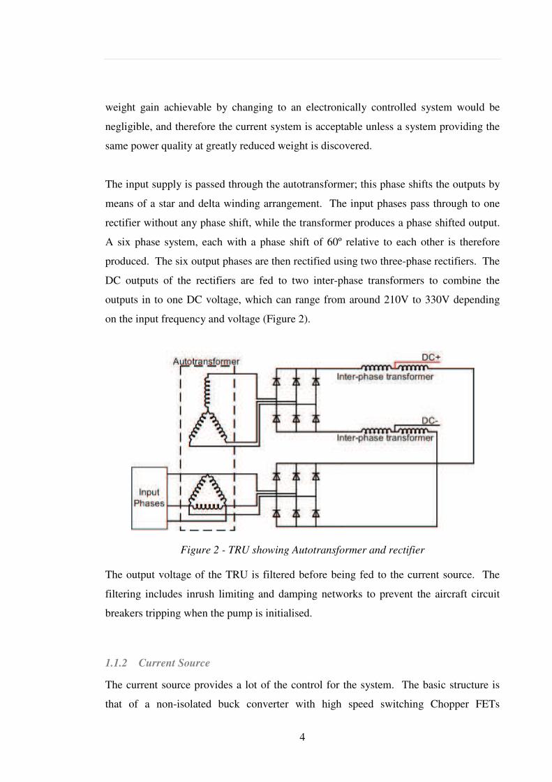
The input supply is passed through the autotransformer; this phase shifts the outputs by
means of a star and delta winding arrangement. The input phases pass through to one
rectifier without any phase shift, while the transformer produces a phase shifted output.
A six phase system, each with a phase shift of 60º relative to each other is therefore
produced. The six output phases are then rectified using two three-phase rectifiers. The
DC outputs of the rectifiers are fed to two inter-phase transformers to combine the
outputs in to one DC voltage, which can range from around 210V to 330V depending
on the input frequency and voltage (Figure 2).
Figure 2 - TRU showing Autotransformer and rectifier
The output voltage of the TRU is filtered before being fed to the current source. The
filtering includes inrush limiting and damping networks to prevent the aircraft circuit
breakers tripping when the pump is initialised.
1.1.2 Current Source
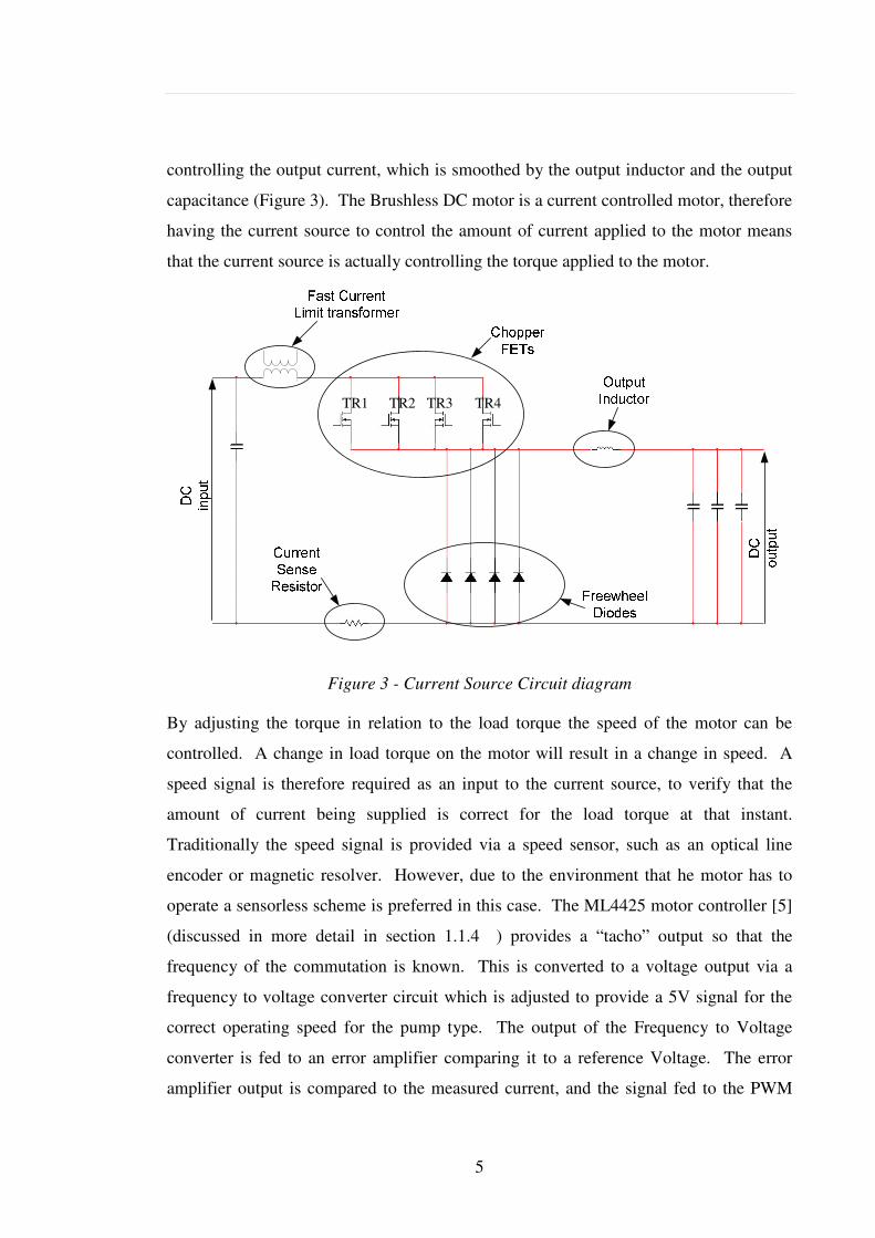
The current source provides a lot of the control for the system. The basic structure is
that of a non-isolated buck converter with high speed switching Chopper FETs
5
controlling the output current, which is smoothed by the output inductor and the output
capacitance (Figure 3). The Brushless DC motor is a current controlled motor, therefore
having the current source to control the amount of current applied to the motor means
that the current source is actually controlling the torque applied to the motor.
Figure 3 - Current Source Circuit diagram
By adjusting the torque in relation to the load torque the speed of the motor can be
controlled. A change in load torque on the motor will result in a change in speed. A
speed signal is therefore required as an input to the current source, to verify that the
amount of current being supplied is correct for the load torque at that instant.
Traditionally the speed signal is provided via a speed sensor, such as an optical line
encoder or magnetic resolver. However, due to the environment that he motor has to
operate a sensorless scheme is preferred in this case. The ML4425 motor controller [5]
(discussed in more detail in section 1.1.4 ) provides a “tacho” output so that the
frequency of the commutation is known. This is converted to a voltage output via a
frequency to voltage converter circuit which is adjusted to provide a 5V signal for the
correct operating speed for the pump type. The output of the Frequency to Voltage
converter is fed to an error amplifier comparing it to a reference Voltage. The error
amplifier output is compared to the measured current, and the signal fed to the PWM
TR1 TR2 TR3 TR4
6
controller (UC1825 PMW controller [6]). The current, and therefore the torque applied
to the motor is adjusted to maintain the output voltage of the F-V converter at 5V.
The chopping for the DC is provided by four high speed FETs [7], which are switched
in paralleled pairs (TR1 and TR2 are one parallel pair, and TR3 and TR4 are the other)
in a push-push configuration. Chopping in this way reduces the conduction losses in the
FETs (as the resistance is halved due to them being in parallel) and allows a near 100%
duty cycle for operation at high loads and low input voltages. The switched DC is
smoothed by an output inductor and the ripple on the output from this is smoothed by
the three output capacitors shown on the right of the diagram (Figure 3).
The brushless DC motor was chosen for the A380 drive as the speed requirements
specified that there should be no more than a 1% speed drift throughout the life of the
pump. This is not achievable with a normal induction motor running open loop
(without controller) directly off the variable frequency supply in the aircraft where the
input can vary from 360 – 800Hz [3]. An induction motor speed varies with load, as the
torque generated is related to the slip between the stator frequency and the rotor speed.
1.1.3 Auxiliary power supply and fault detection
The auxiliary power supply generation uses the high Voltage DC to generate all the
power supply rails for the rest of the system, including three floating supplies required
for the upper gate drives in the motor drive bridge, and the supplies for the control ICs.
The unit also enables the current source switching once all required power supply rails
are present.
The fault detection is required for protection of the system. This includes detection of a
missing input phase, and speed fault detection that may cause pressure problems within
the fuel system such as pressure pulses. The missing phase detection is achieved by
having sense windings built in to the Transformer Rectifier Unit (TRU) which provide a
low voltage signal detection of the three input phases. This is rectified, and used to
determine whether all three phases are present. The level of the rectified signal is also
used to determine whether a low mains condition is occurring. The speed fault signal is

7
masked during the low mains and missing phase conditions, as this will cause the speed
to drop, but is not due to a fault in the speed control of the motor. If a fault occurs
meaning that the motor does run outside the speed conditions, and the speed fault is
triggered, the unit disables the current source, and latches in this state requiring the
mains input to be cycled to re-enable it.
1.1.4 Motor Drive
The motor drive uses a motor control IC to commutate the Brushless DC motor (BLDC)
using sensorless control. The Fairchild ML4425 is used to provide the drives to an
IGBT bridge (Figure 4), which is used to direct the current produced by the current
source to the correct windings of the motor, and at present is the only IC offering
sensorless control in this manner.
Figure 4 - Motor drive bridge
The ML4425 is not available over the required temperature range for operation between
-55˚C and +125˚C (maximum manufacturers specified temperature range is for the
industrial version, and is between -40˚C and +85˚C [5]). To ensure that the operation
over the required extended temperature range was acceptable, a large amount of
characterisation of the controller was undertaken by Eaton using their in-house
environmental facilities. This information is only available as an internal document
within Eaton, and hence has not been cited as a reference.
Having characterised the operation over the -55˚C to +125˚ operating conditions, it was
recorded that the tolerances seen on the internal voltage and current sources (used for
8
timings during the commutation and current control) had large variations from IC to IC.
Due to this, the current control by way of switching the IGBTs that the ML4425 can
provide would have had too larger tolerance to provide the 1% speed variation over life
that is required. To facilitate the tighter speed requirement the current source was
introduced to the Eaton motor drive to provide the current and speed control. The
ML4425 was retained purely to provide the commutation and start up sequence to the
motor. The commutation requirements and sensorless scheme employed will be
discussed further in later sections of this thesis.
1.1.5 Rationale for Implementation using a Current Source
The space constraints for the Eaton designed A380 drive outlined in the previous
sections was particularly restrictive. The requirement was to provide an inverter to
maintain a constant pump speed from the variable frequency aircraft supply. The
necessity for a motor controller embedded in a fuel pump, and contained within a fuel
tank environment was perceived to require a non-standard approach to the motor drive.
The traditional use of a chopped motor bridge was not easily achievable with the motor
controller chosen (ML4425 motor drive IC) as the variability across production batches
and temperature was not accurate enough to guarantee the 1% speed change over the
life of the pump. A more accurate scheme to control the current was therefore required,
allowing the ML4425 to simply provide the start up sequence to the motor bridge, and
perform the commutation under sensorless operation once the motor was running. The
high accuracy current control required was then achievable using high quality, low
temperature coefficient devices in the current source control.
The choice of a current source controller over the chopped bridge was also influenced
by the misplaced belief that an output filter would be required between each phase of
the drive and the motor should a chopped bridge be employed. The size of a three-
phase filter would increase the weight and space required (having both inductors and
capacitors) for the drive, and would push the electronics beyond the space envelope
available. The inductance of the motor acts to smooth the switched waveform applied
to it, and is generally large enough to remove the switching frequency from the current
in to the motor, so the output filter is not necessary.

9
The motor design would not meet the dv/dt requirements if a high speed MOSFET
chopping bridge was employed directly to the windings, as the wire insulation is not
adequate. It is however adequate for a slower switching IGBT bridge to be applied
directly to the windings. A scheme has been identified (for another project bid) that
would allow a MOSFET bridge to be employed at a similar frequency to the A380
current source (250 kHz) with minimal change to the motor design. An additional layer
of insulation would be required along the first winding of each motor phase to increase
the dv/dt that it can withstand [8]. This is only required on the first turn of the winding,
as the inductance begins to limit the rate of change that the rest of the winding
experiences. This has not been used on any current projects, and is not used in the
context of the research presented in this thesis.

10
Chapter 2. Sensorless Control Schemes
Control schemes for the commutation of a permanent magnet DC motor can be broken
down in to two categories depending on the applied current shape and back EMF
voltage shape generated. The current applied to drive a permanent magnet motor can be
either sinusoidal or square wave. To distinguish the two, the sinusoidally driven motor
will be referred to as a Permanent Magnet Synchronous Machine (PMSM), and the
square wave will be referred to as a Brushless DC Machine (BLDC).
The motor being studied in this thesis has already been referred to as a Brushless DC
motor, as this is fed by square wave current commutation.
2.1 Rotor Position Requirements
Both the BLDC and PMSM motors are synchronous machines, so for optimum torque
production the commutation of the stator windings must be synchronised with the
position of the rotor. In a traditional control scheme, this information would be
determined from a rotor encoder or resolver. This allows maximum torque production
from standstill, and also allows full torque operation at zero speed.
The motors used in aircraft fuel pumps are often fuel flooded to provide cooling to the
motor windings. This means that the entire stator and rotor are immersed in the fuel,
and provide the flow through the motor due to the action of the impeller.
This environment is generally inhospitable to the inclusion of encoders, and the
construction of a dry area that is more suited to them requires the inclusion of fuel seals
both increase the load on the motor, and cannot be guaranteed for the life of the aircraft.
The use of an encoder in a fuel flooded environment has few advantages over a
sensorless controller.

11
2.2 Rotor Position Determination
A number of schemes for determining the rotor position from measurable and
determinable quantities exist. An overview of the most commonly researched is
discussed in the following sections.
2.2.1 Inductance Variation
The rate of change of current in a winding is dependant on the inductance of that
winding. The inductance is a function of winding current and rotor position. With a
permanent magnet rotor passing the winding, the inductance will vary due to the
magnetic field of the rotor [9][10][11][12][13][14][15][16]. Therefore, monitoring the
rate of change of current in the winding, the rotor position can be determined. This has
an advantage over some other sensorless schemes in that it can be useful for zero-speed
position detection. Using an inductance variation scheme can be compromised by three
factors:
1. The rate of change of current in the winding is dominated by the motional EMF
generated by the permanent magnets.
2. The variation in inductance occurs twice per electrical cycle, which may cause
ambiguity in the sensed position.
3. Rotors with surface mounted magnets do not have saliency, so any variation in
the inductance will be caused by magnetic saturation.
As stated previously, inductance variation can be used to determine the rotor position at
standstill; this has great benefits in applications such as traction where a reverse
movement due to an aligning pulse would not be acceptable.
Experiments with position estimation at standstill have been performed for applications
such as traction with exploratory voltage pulses being applied to all of the phase
windings of a salient rotor permanent-magnet machine, with the resulting current pulses
being used to determine the position of the rotor. This, however still leaves the
ambiguity as explained in the second point. The rotor position can be in one of two
positions.
The resulting incremental inductance in
has a low at both 0º and 180º (results shown are fo
machine). Research by Nakashima et al
determine which position the rotor is in, 0º or 180
to the winding with the rotor aligned at 0º has the
flux linked by that phase.
Figure 5 – Permanent
12
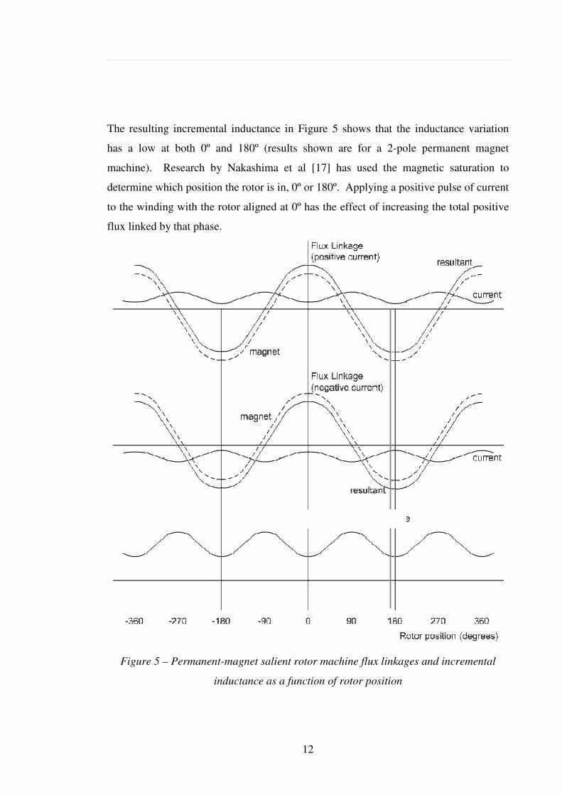
The resulting incremental inductance in Figure 5 shows that the inductance variation
has a low at both 0º and 180º (results shown are for a 2-pole permanent ma
machine). Research by Nakashima et al [17] has used the magnetic saturation to
determine which position the rotor is in, 0º or 180º. Applying a positive pulse of current
to the winding with the rotor aligned at 0º has the effect of increasing the to
flux linked by that phase.
Permanent-magnet salient rotor machine flux linkages and incr
inductance as a function of rotor position
Incremental inductance
shows that the inductance variation
pole permanent magnet
has used the magnetic saturation to
º. Applying a positive pulse of current
effect of increasing the total positive
magnet salient rotor machine flux linkages and incremental
Incremental inductance
13
If the rotor is aligned at 180º, the positive current pulse will reduce the total negative
flux linkage. The positive and negative flux linkages will therefore be at different
amplitudes, and hence a different level of magnetic saturation. An increase in magnetic
saturation will be seen as lower incremental inductance and hence the amplitude of the
current pulse will be greater in one of the two positions. This can then be used to
determine the position of the rotor, although Nakashima et al have reported accuracy of
only 18º.
2.2.2 High Frequency Injection
Whilst considered by some as a separate method of position estimation, the basic
concept behind high frequency injection is the same as inductance variation. The rotor
starting position can be investigated by applying a high frequency, low amplitude signal
to the stator windings, and detecting the position dependant incremental inductance
[18][19][20][21][22][23][24][25][26]. A 50Hz, low amplitude PWM signal was used
by Noguchi et al [27], and the winding impedance evaluated. By adjusting the current
controller’s parameters, an oscillatory behaviour was generated for the lowest values of
incremental impedance. This relates to the maximum magnetic saturation, and hence
the ambiguity between the 0° and 180° positions can be removed. A higher frequency
(500Hz) was used by Aihara et al [19] and discrimination between rotor positions
determined by magnetic saturation effects.
Using high frequency injection for continuous running salient rotor permanent magnet
machines has been used with two techniques:
Corley and Lorenz [28] used a 2kHz carrier frequency to inject a Voltage signal, and
measured the frequency component of the current, which was modulated by the rotor
position. The signal was compared to a signal of equal carrier frequency but modulated
by a motor estimator. The error signal generated by comparing the two was then used
to adjust the motor estimator and track the actual rotor position. This technique has
been demonstrated over a large speed range, including zero speed.
14
Kulkarni and Ehsani [29] calculated the effective phase inductance from the behaviour
of a hysteresis current controller. Assumptions were made that the motor was always
spinning in one direction, and the ambiguity of rotor position removed by always
starting from a known position.
Improvements in the inductance variation technique can be made by adding a short-
circuited winding to a surface mounted magnet rotor, which would normally have no
saliency. The winding increases the position dependence of the winding inductance and
therefore makes inductance variation possible with a non-salient rotor.
High frequency injection has been a strong area of research, particularly for the
University of Wuppertal [22][23][24]. Petrovi, Stankovi and Blaško [30] have
explored the idea of using a high frequency carrier wave by making use of the high
frequency component of the PWM signal instead of applying a separate high frequency
wave to the machine.
2.2.3 Flux Linkage Estimation
Flux linkage in permanent magnet machine can be simplified to the equation:
dt
dRiv
ψ+= (1)
where:
v = phase terminal Voltage
i = phase current
R = phase resistance
ψ = phase flux linkage
Re-arranging this equation to give:
−= dtRiv )(ψ (2)
15
Therefore, with a powerful enough processor, a real time estimation of the flux linkage
is obtainable from the phase voltage and Ri drop [31]. Using (2), a continuous estimate
of the phase flux linkage is produced. Using an open loop integrator in this way leaves
the system prone to integrator drift and integrator saturation over time [18].
In industrial applications, measurement of phase terminals is not always practical
because of requirements for isolation. In cases where this is applicable, the phase
voltage can be determined from the DC supply and the modulation index applied to it.
The use of the DC voltage and demanded voltage on that does not necessarily take in to
account the error that the introduction of dead-time required on the bridge switching.
This will tend to be greatest when the demanded voltage is close to zero, as the dead-
time proportionally increases with respect to the modulation index. Using a digital
controller allows the dead-time to be known, and so a correction factor can be achieved.
This error has been noted by a number of authors, who have compensated for the dead-
time error [18] [32] [33].
Replacing the open loop integrator with a low pass filter or alternative integrator can
reduce the drift. Modifying the system in this way can improve the overall
performance, but may degrade the low speed operation. A closed loop system is more
applicable and has been the focus of more recent research [34].
2.2.3.1 Mechanical Model for Flux Estimation
In a BLDC, motor the flux linkage due to the permanent magnets is a trapezoidal
function of position. In a PMSM, the variation of flux linkage must also be sinusoidal.
The flux linkage is a function of the permanent magnet and the current flowing in that
winding. As previously noted, the inductance variation, and hence the flux linkages for
a phase are dependant on the machine construction [18][35][36][37]. A mechanical
model of the motor is used, requiring knowledge of the mechanical inertia (J), viscous
friction (B), and load torque (TL).
16
)(1
LTBTJdt
d−−= ω
ω (3)
ωθ
=dt
d (4)
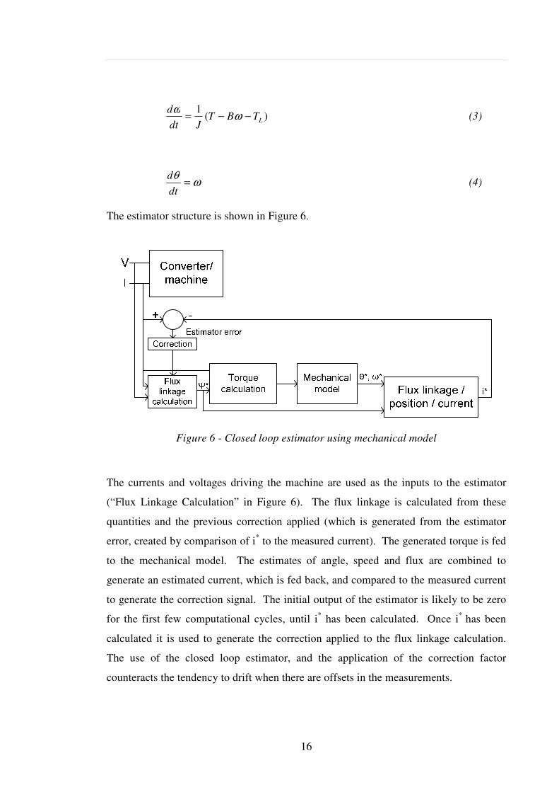
The estimator structure is shown in Figure 6.
Figure 6 - Closed loop estimator using mechanical model
The currents and voltages driving the machine are used as the inputs to the estimator
(“Flux Linkage Calculation” in Figure 6). The flux linkage is calculated from these
quantities and the previous correction applied (which is generated from the estimator
error, created by comparison of i* to the measured current). The generated torque is fed
to the mechanical model. The estimates of angle, speed and flux are combined to
generate an estimated current, which is fed back, and compared to the measured current
to generate the correction signal. The initial output of the estimator is likely to be zero
for the first few computational cycles, until i* has been calculated. Once i* has been
calculated it is used to generate the correction applied to the flux linkage calculation.
The use of the closed loop estimator, and the application of the correction factor
counteracts the tendency to drift when there are offsets in the measurements.
17
Use of a mechanical model is not desirable, despite results produced by Terzic and
Jadric [33] with operation down to speeds of 50 rpm. The mechanical model requires
that the motor parameters (inertia, viscous friction and load torque) must be available
before starting, these parameters have a tendency to drift and change with temperature,
and therefore the model becomes inaccurate for the motor at that time leading to
positional inaccuracy and a reduction in efficiency. Terzic and Jadric [33] also
introduced a winding resistance calculation, as this varies with temperature and creates
errors in the flux linkage estimation.
2.2.3.2 Flux Estimation without Mechanical Model
Wu and Slemon investigated the flux linkage without a mechanical model for a
sinusoidal machine without saliency [38]. This was implemented using a hysteresis
controller and external analogue integrators for the flux linkage estimation. To ensure
that the average flux linkage in each phase is zero, an offset voltage is generated to
counteract the drift of the analogue integrators. This approach resulted in accurate
steady state running, but was ineffective to fast changes in load or speed, and did not
allow the motor to self-start.
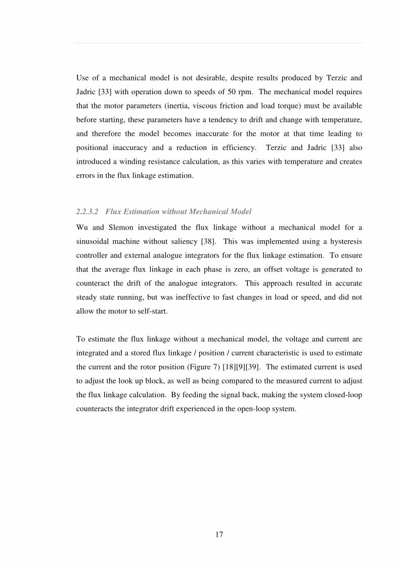
To estimate the flux linkage without a mechanical model, the voltage and current are
integrated and a stored flux linkage / position / current characteristic is used to estimate
the current and the rotor position (Figure 7) [18][9][39]. The estimated current is used
to adjust the look up block, as well as being compared to the measured current to adjust
the flux linkage calculation. By feeding the signal back, making the system closed-loop
counteracts the integrator drift experienced in the open-loop system.
18
Figure 7 - Closed loop observer without mechanical model
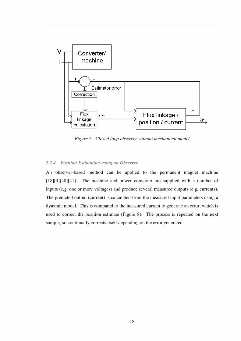
2.2.4 Position Estimation using an Observer
An observer-based method can be applied to the permanent magnet machine
[18][9][40][41]. The machine and power converter are supplied with a number of
inputs (e.g. one or more voltages) and produce several measured outputs (e.g. currents).
The predicted output (current) is calculated from the measured input parameters using a
dynamic model. This is compared to the measured current to generate an error, which is
used to correct the position estimate (Figure 8). The process is repeated on the next
sample, so continually corrects itself depending on the error generated.
19
Figure 8 - Observer method for position estimation
This approach has been adopted by International Rectifier for their range of sensorless
AC motor control devices [42].
2.2.5 BEMF zero crossing detection
The Fairchild ML4425 sensorless brushless dc motor controller is currently used by
Eaton Aerospace to commutate the BLDC motor that is employed in the Airbus A380
drive. This device uses the BEMF zero crossing detection technique to determine the
rotor position [37][43][44][45][46][47][48][49][50][51][52][53]
[54][55][56][57][58][59][60][61]. A BLDC motor is commutated so that only two
windings are energised at one time (Figure 9). The third winding is not energised, but
has a Voltage induced in it due to the permanent magnet rotor passing it. The level of
back EMF is proportional to the speed of the rotor.
ωekV = (5)
The ML4425 operates by gating the signal for the non-fed phase. The BEMF crossing
occurs on each phase twice per electrical cycle, meaning that six crossings can be
detected during one electrical cycle for a three-phase machine.
20
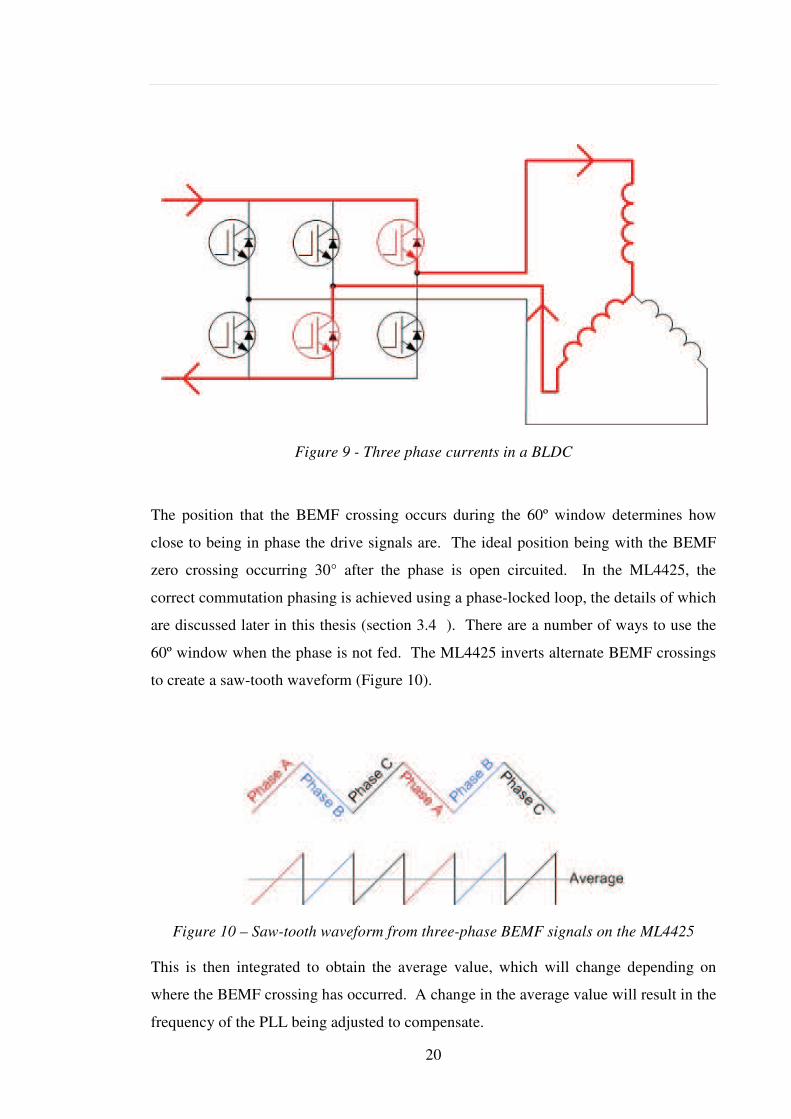
Figure 9 - Three phase currents in a BLDC
The position that the BEMF crossing occurs during the 60º window determines how
close to being in phase the drive signals are. The ideal position being with the BEMF
zero crossing occurring 30° after the phase is open circuited. In the ML4425, the
correct commutation phasing is achieved using a phase-locked loop, the details of which
are discussed later in this thesis (section 3.4 ). There are a number of ways to use the
60º window when the phase is not fed. The ML4425 inverts alternate BEMF crossings
to create a saw-tooth waveform (Figure 10).
Figure 10 – Saw-tooth waveform from three-phase BEMF signals on the ML4425
This is then integrated to obtain the average value, which will change depending on
where the BEMF crossing has occurred. A change in the average value will result in the
frequency of the PLL being adjusted to compensate.
21
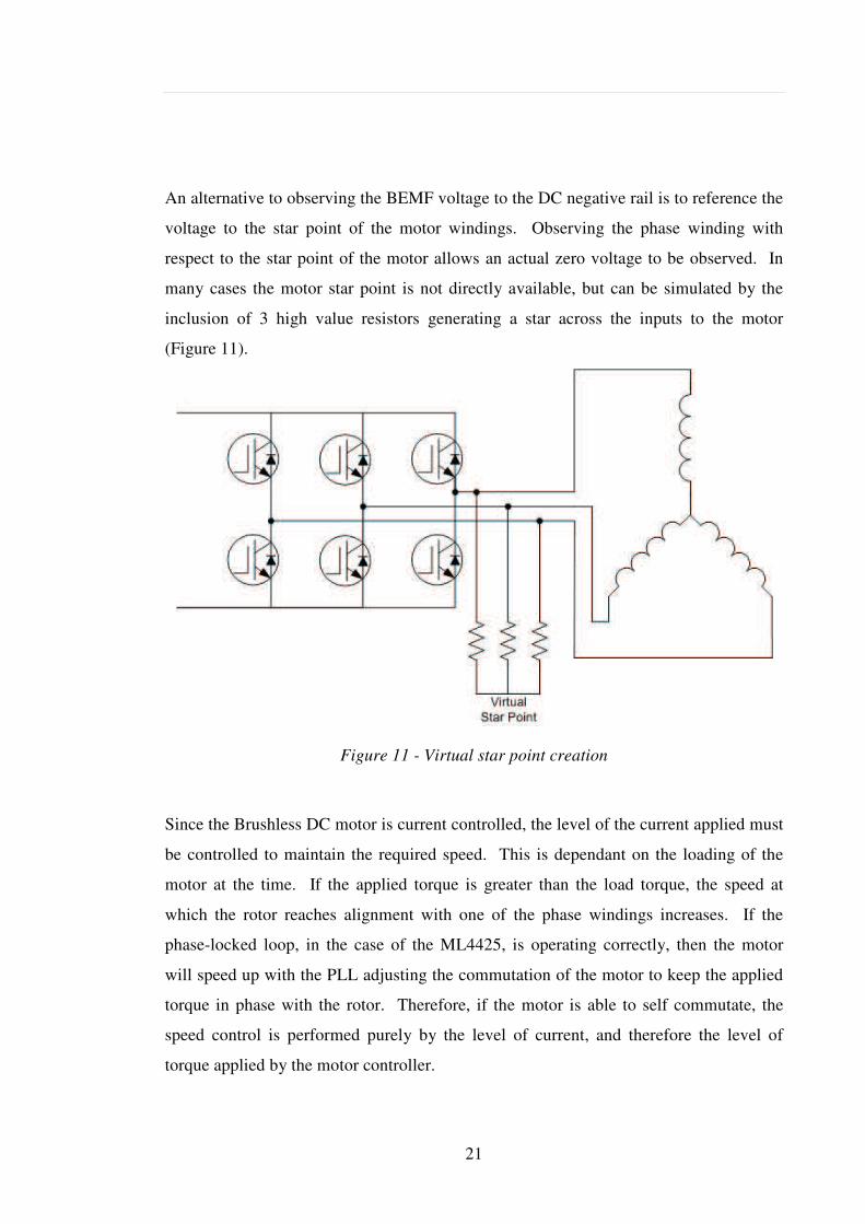
An alternative to observing the BEMF voltage to the DC negative rail is to reference the
voltage to the star point of the motor windings. Observing the phase winding with
respect to the star point of the motor allows an actual zero voltage to be observed. In
many cases the motor star point is not directly available, but can be simulated by the
inclusion of 3 high value resistors generating a star across the inputs to the motor
(Figure 11).
Figure 11 - Virtual star point creation
Since the Brushless DC motor is current controlled, the level of the current applied must
be controlled to maintain the required speed. This is dependant on the loading of the
motor at the time. If the applied torque is greater than the load torque, the speed at
which the rotor reaches alignment with one of the phase windings increases. If the
phase-locked loop, in the case of the ML4425, is operating correctly, then the motor
will speed up with the PLL adjusting the commutation of the motor to keep the applied
torque in phase with the rotor. Therefore, if the motor is able to self commutate, the
speed control is performed purely by the level of current, and therefore the level of
torque applied by the motor controller.

22
2.3 Justification for choosing BEMF detection
While the BEMF sensing scheme is not the most technically advanced, it does have
some advantages over other schemes evaluated:
• The scheme is already in use as the analogue ML4425 used in the existing A380
drive, and is therefore a known technology to the aerospace industry. This also
makes it Eaton’s preferred choice, as much of the knowledge already gained
from the production version of the A380 drive can be re-used.
• There have been no reported occurrences of in-service pumps having stability or
reliability issues due to the sensorless control scheme employed. It is therefore
considered robust and reliable by the customer. This confidence has taken a
number of years to be established, and a change to the control scheme would
require a similar maturity to be considered robust by the customer.
• The possibility of creating a relatively low complexity software implementation
of the BEMF sensing scheme would mean that the FAA and EASA qualification
of the electronics under DO-254 (Design Assurance Guidance for Airborne
Electronic Hardware) [62] would be simplified as the system could be defined as
a “simple” system. This would not be the case with the system implemented on
a DSP, as this would be considered complex hardware, but by keeping the
processing required by the DSP as low as possible may enable implementation
on a lower complexity device (e.g. a COTS Microprocessor, which does not
require DO-254 certification).
• DO-178 (Software Considerations in Airborne Systems and Equipment
Certification) [63] would be applicable, as virtually all software is considered
complex. This is unavoidable in the use of a software programmable device.
Alternatively, if the control scheme could be implemented in purely hardware,
the design could be transferred to an FPGA device, therefore removing the need
for DO-178 qualification.
Qualification programs add a large amount of cost to any development programs, so any
reduction possible constitutes a major cost saving for the company, and DO-178 is
renowned within the industry as the most arduous of the qualification criteria. The
OEM market within the commercial aerospace business is highly competitive, with

23
margins being very small or none existent (many OEM programmes run at a loss, with
the aftermarket spares and repairs business providing a much greater levels of
profitability). The use of software within a fuel pump, and its associated qualification
requirements would make the pump uncompetitive in the market. As the aerospace
market increases its desire for fault reporting to the aircraft (via ARINC interfaces,
based on CAN network) the use of software will increase. During the research carried
out within this thesis, this was not considered a high priority, and keeping the
complexity and cost of the system low was more desirable. The use of control scheme
already in service, albeit implemented using a different platform, is less likely to require
additional testing and qualification than a different implementation.
While the overall aim of the implementation from Eaton’s point of view is to produce a
system that would meet qualification requirements for the aerospace industry, a DSP
controller will be used for the development of the hardware, using a software
implementation of the solution. This will allow a flexible approach to the
implementation with the use of high level language programming (C code
implementation). A translation to COTs microprocessor, FPGA, or hardware only
based system would then be easily achievable once a finalised solution has been
reached.
The decision to implement the BEMF zero-crossing detection scheme is therefore partly
a commercial one (due to costs of implementing a scheme requiring software) and an
engineering one to allow re-use of knowledge already gained from Eaton’s previous
development.
2.4 Sensorless Control for Different Motor Types
Sensorless control schemes for induction motors and switched reluctance motors have
been of great interest during recent years. While accurate sensorless speed control is
now achievable, the size and relatively low power density in comparison to the
permanent magnet motor means that the induction motor is not a viable alternative to
BLDC motor used in the A380 motor controller. The relative weight and noise of the
switched reluctance motor compared to the brushless DC also make this motor type less

24
suited to the aircraft fuel pump. The sensorless techniques for induction motors and
switched reluctance motors have been investigated as a reference against the relative
performance to the brushless dc control schemes. While some cross over between
techniques used for the sensorless control of both the induction motor and the switched
reluctance motor these will not be discussed in this thesis, but are sited as references to
relevant techniques that may be of interest. [12]
[64][65][66][67][68][69][70][71][72][73][74]
2.5 Alternative Converter Topologies
The choice of an external current source for the Eaton drive allows the possibility of
alternative converter topologies to be explored. A range of different converter
topologies will be discussed and critically analysed, allowing the most appropriate
converter for an aerospace application to be selected. The analysis of converter
topologies was specifically requested by Eaton to ensure that future development plans
would focus on the correct technology path. The external current source topology is
included in the analysis, but is not discussed in depth during this section as it has
previously been described (Section 1.1.2 ).
2.5.1 Matrix Converters
The matrix converter has been an area of much research over the past twenty years or
so. The full matrix topology (Figure 12) allows bidirectional power flow within the
converter by the use of 9 bidirectional switches that connect the input phase to the
output phases to produce the desired frequency and voltage (up to 86% of the input
voltage) [75][76][77].
25
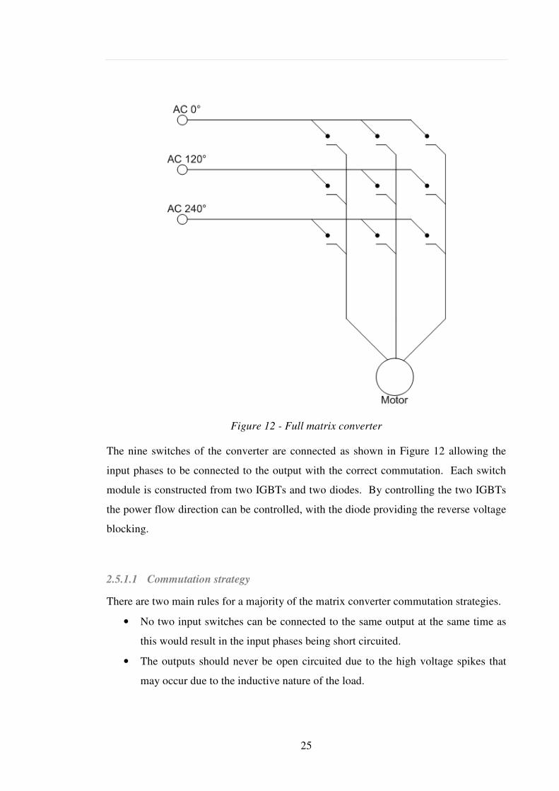
Figure 12 - Full matrix converter
The nine switches of the converter are connected as shown in Figure 12 allowing the
input phases to be connected to the output with the correct commutation. Each switch
module is constructed from two IGBTs and two diodes. By controlling the two IGBTs
the power flow direction can be controlled, with the diode providing the reverse voltage
blocking.
2.5.1.1 Commutation strategy
There are two main rules for a majority of the matrix converter commutation strategies.
• No two input switches can be connected to the same output at the same time as
this would result in the input phases being short circuited.
• The outputs should never be open circuited due to the high voltage spikes that
may occur due to the inductive nature of the load.
26
2.5.2 Reduced Matrix Converter
For the application of an aircraft fuel pump a unidirectional power flow is sufficient and
in many cases desirable as a reverse power flow may introduce distortion to the supply
grid which can impact the performance of other equipment connected to it. This is
particularly true of the variable frequency system, as the converter would have to ensure
the frequency being applied to the supply was the same as it.
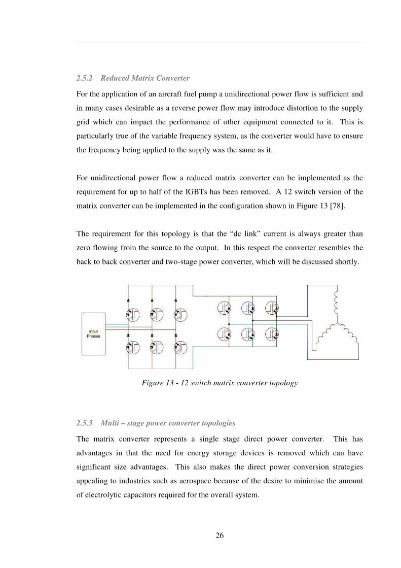
For unidirectional power flow a reduced matrix converter can be implemented as the
requirement for up to half of the IGBTs has been removed. A 12 switch version of the
matrix converter can be implemented in the configuration shown in Figure 13 [78].
The requirement for this topology is that the “dc link” current is always greater than
zero flowing from the source to the output. In this respect the converter resembles the
back to back converter and two-stage power converter, which will be discussed shortly.
Figure 13 - 12 switch matrix converter topology
2.5.3 Multi – stage power converter topologies
The matrix converter represents a single stage direct power converter. This has
advantages in that the need for energy storage devices is removed which can have
significant size advantages. This also makes the direct power conversion strategies
appealing to industries such as aerospace because of the desire to minimise the amount
of electrolytic capacitors required for the overall system.
27
The full matrix converter consists of x number of input phases and y number of output
phases. This requires the number of switches to be x*y. A number of multi-stage
topologies exist which also have no energy storage capacitors but also have some
advantages over other converters.
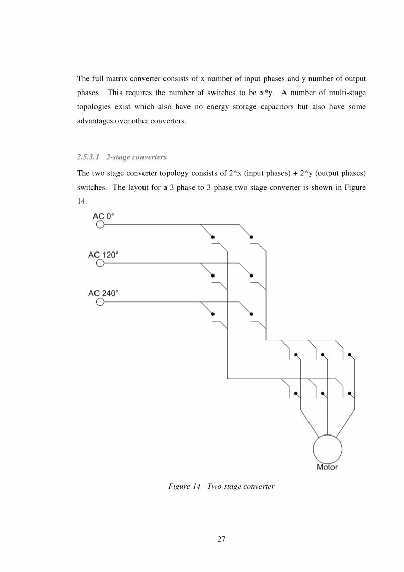
2.5.3.1 2-stage converters
The two stage converter topology consists of 2*x (input phases) + 2*y (output phases)
switches. The layout for a 3-phase to 3-phase two stage converter is shown in Figure
14.
Figure 14 - Two-stage converter
28
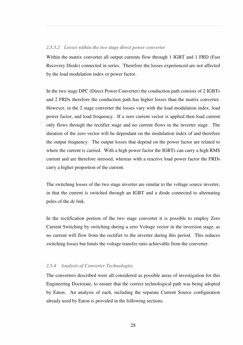
2.5.3.2 Losses within the two stage direct power converter
Within the matrix converter all output currents flow through 1 IGBT and 1 FRD (Fast
Recovery Diode) connected in series. Therefore the losses experienced are not affected
by the load modulation index or power factor.
In the two stage DPC (Direct Power Converter) the conduction path consists of 2 IGBTs
and 2 FRDs therefore the conduction path has higher losses than the matrix converter.
However, in the 2 stage converter the losses vary with the load modulation index, load
power factor, and load frequency. If a zero current vector is applied then load current
only flows through the rectifier stage and no current flows in the inverter stage. The
duration of the zero vector will be dependant on the modulation index of and therefore
the output frequency. The output losses that depend on the power factor are related to
where the current is carried. With a high power factor the IGBTs can carry a high RMS
current and are therefore stressed, whereas with a reactive load power factor the FRDs
carry a higher proportion of the current.
The switching losses of the two stage inverter are similar to the voltage source inverter,
in that the current is switched through an IGBT and a diode connected to alternating
poles of the dc link.
In the rectification portion of the two stage converter it is possible to employ Zero
Current Switching by switching during a zero Voltage vector in the inversion stage, as
no current will flow from the rectifier to the inverter during this period. This reduces
switching losses but limits the voltage transfer ratio achievable from the converter.
2.5.4 Analysis of Converter Technologies
The converters described were all considered as possible areas of investigation for this
Engineering Doctorate, to ensure that the correct technological path was being adopted
by Eaton. An analysis of each, including the separate Current Source configuration
already used by Eaton is provided in the following sections.
29
2.5.4.1 Matrix Converters
While these are an area of research, there are few areas where the reliability and benefits
of using these over a conventional converter can be observed. While the airline industry
likes to be seen to be pushing technology forward, safety and reliability are always
much more of a driver. The variable frequency input, to become standard on many
aircraft, complicates the control of the matrix converter. The control algorithm must be
able to adjust itself to changing input frequency. This is likely to require use of a high
powered software driven controller, as the overhead for implementing in hardware alone
would be large. This would dramatically increase the cost of the development and
qualification programme, and would push the costs beyond what is considered
acceptable for fuel pump application. The use of matrix converts may become more
common place but is currently perceived as a step too far for the aircraft manufacturers.
The 86% output voltage achievable by the matrix converter provides less output voltage
than is currently achieved from the current source topology, and would therefore reduce
the operating range of the drive.
2.5.4.2 Multi-stage Power Converters
The multi-stage power converter effectively provides a standard motor bridge from a dc
link, as with a standard motor drive. The addition of an active front end to provide this
DC does not provide a great enough benefit over the passive autotransformer TRU
scheme already employed. Weight and cost estimates (including cooling of the power
devices in the rectification stage) have suggested that there would be little benefit in
using an active rectifier over the current 12-pulse autotransformer system, and may have
a detrimental effect on the reliability figures that can be calculated for the system as
electronic devices are perceived to be unreliable when compared to magnetics.
2.5.4.3 Separate Current Source (Eaton A380 drive)
The use of a separate current source has allowed a highly accurate speed controlled
drive to be produced using only analogue control. The implementation means that the
output of the motor drive has a smooth current rather than a chopped waveform. This
would allow the controller to be used with a remote motor, as well as the close coupled

30
motor that it is currently applied to without greatly increased radiated noise problems.
The use of an extra converter stage (current source) reduces the losses experienced in
the drive bridge itself, which become dominated by the conduction losses of the IGBTs.
However, there are additional losses introduced by the switching components in the
current source. Analysis has shown that the combination of conduction and switching
losses for the separate current source is higher than that of the switched bridge
configuration.
2.5.4.4 Six Switch Bridge
The standard six switch bridge is well known in all industries, and is a well proven
technology making it readily acceptable for aircraft manufacturers. Most controllers
(DSPs, FPGAs, etc.) designed for motor applications will have six-switch bridge
capability. The standard bridge will therefore be employed to maximise the choice of
controllers.
2.6 Simulation
The aerospace industry standard simulation package is Saber, produced by Synopsys.
Simulations of the ML4425 based system were run varying the loading characteristics
and the application of the PWM control. The model and simulation results can be seen
in Appendix 5.
The simulation allows the PWM control to be applied directly to the bridge by disabling
the current source section and utilising the PWM capabilities of the ML4425 model. As
the Saber model is representative of the ideal version of the motor controller there is no
variability in controllers, as characterised by Eaton over a sample batch of ML4425s.
The wide range of PWM duty cycles for identical inputs made using the current
controlling capability of the ML4425 unviable for a production version.
Adjusting the switching frequency of the Saber model to match the DSP controller
being used allowed the model to represent the system to be implemented in the DSP
controller. The motor start up characteristics seen from the simulation can then be
extrapolated from this
the current source in the Eaton design. As this pr
would be performed by the bridge modulation in the
performance of both the current source model a
evaluated from the same model. A
can be concluded to have minimal effect on the perf
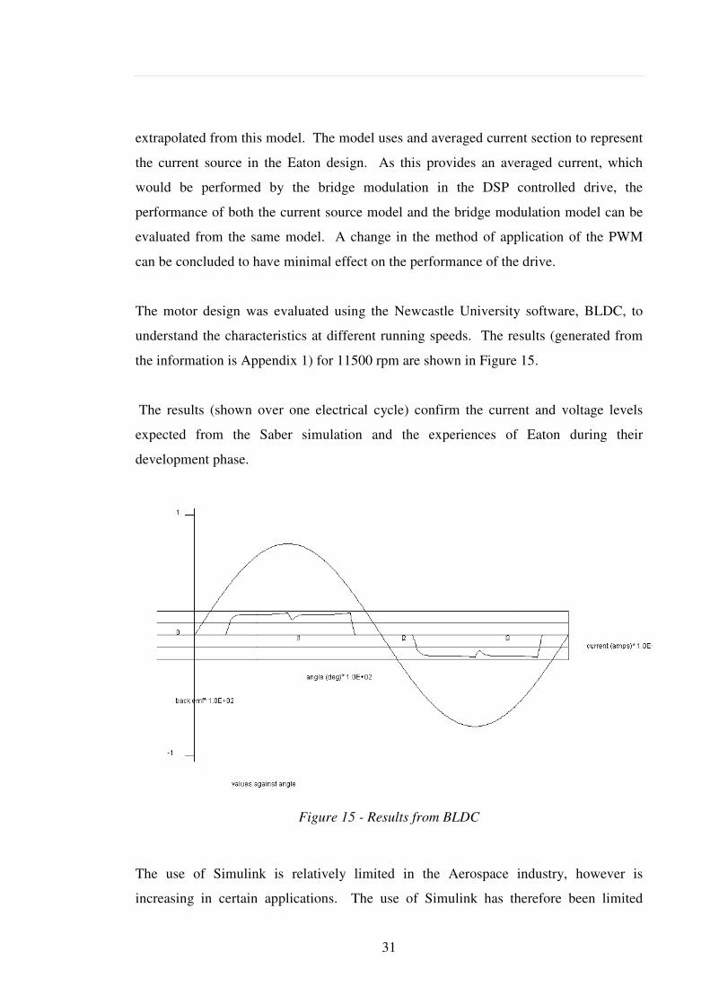
The motor design was
understand the characteristics at different running
the information is Appendix
The results (shown over one electric
expected from the Saber simulation and the experien
development phase.
The use of Simulink is relatively limited in the Ae
increasing in certain applications. The use of Sim
31
extrapolated from this model. The model uses and averaged current section to represent
the current source in the Eaton design. As this provides an averaged current, which
would be performed by the bridge modulation in the DSP controlled drive, t
performance of both the current source model and the bridge modulation model
evaluated from the same model. A change in the method of application of the PWM
can be concluded to have minimal effect on the performance of the drive.
as evaluated using the Newcastle University s
understand the characteristics at different running speeds. The results
Appendix 1) for 11500 rpm are shown in Figure
The results (shown over one electrical cycle) confirm the current and voltage levels
expected from the Saber simulation and the experiences of Eaton during their
Figure 15 - Results from BLDC
The use of Simulink is relatively limited in the Aerospace industry, however is
increasing in certain applications. The use of Simulink has therefore been limited
uses and averaged current section to represent
ovides an averaged current, which
DSP controlled drive, the
nd the bridge modulation model can be
change in the method of application of the PWM
ormance of the drive.
evaluated using the Newcastle University software, BLDC, to
results (generated from
Figure 15.
al cycle) confirm the current and voltage levels
ces of Eaton during their
ospace industry, however is
ulink has therefore been limited

32
during this doctorate, but has been applied to verify some calculations (e.g. section
3.4.1.1.1).
2.7 Summary
The sensorless control schemes have been discussed and the BEMF zero crossing
detection implementation has been selected as the most robust starting point for the
development of the converter due to its existing usage on aeroplanes. The converter
topology has been analysed and the standard six switch bridge will be utilised. The
current source presently used by Eaton introduces unnecessary losses that are reduced
by modulation of the bridge switches. The differences between the current source
implementation and the bridge modulation implementation have been compared and
found to have inconsequential differences through simulation using Saber.
33
Chapter 3. Converter Implementation
The environment that the motor controller is subjected to on an aircraft presents some
difficult challenges compared to those that are purely ground based. The different
approaches and techniques to allow a processor based motor controller that were used
during the development of hardware through out this doctorate are discussed in the
following chapter.
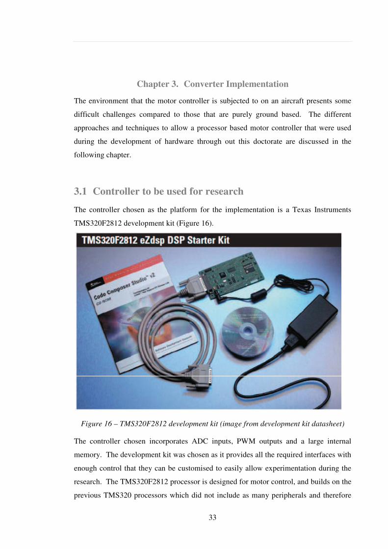
3.1 Controller to be used for research
The controller chosen as the platform for the implementation is a Texas Instruments
TMS320F2812 development kit (Figure 16).
Figure 16 – TMS320F2812 development kit (image from development kit datasheet)
The controller chosen incorporates ADC inputs, PWM outputs and a large internal
memory. The development kit was chosen as it provides all the required interfaces with
enough control that they can be customised to easily allow experimentation during the
research. The TMS320F2812 processor is designed for motor control, and builds on the
previous TMS320 processors which did not include as many peripherals and therefore
34
required additional hardware. The speed of the processor is also greatly improved over
earlier 320 series processors, with the 2812 operating at 150 MHz. The board also has
flash memory available so that the system can be stand alone without the need for a PC
link to load the code to the processor. This would allow the drive to be minimised and
possibly built in to a pump for final demonstration [79].
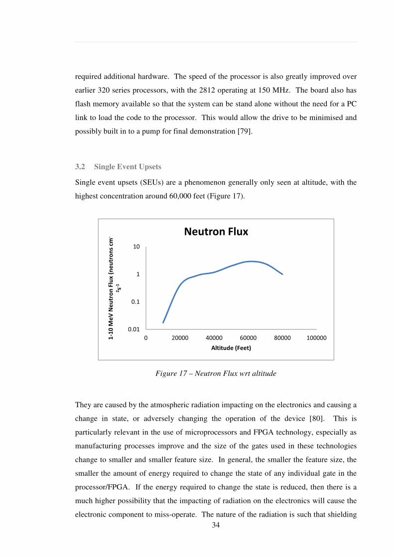
3.2 Single Event Upsets
Single event upsets (SEUs) are a phenomenon generally only seen at altitude, with the
highest concentration around 60,000 feet (Figure 17).
Figure 17 – Neutron Flux wrt altitude
They are caused by the atmospheric radiation impacting on the electronics and causing a
change in state, or adversely changing the operation of the device [80]. This is
particularly relevant in the use of microprocessors and FPGA technology, especially as
manufacturing processes improve and the size of the gates used in these technologies
change to smaller and smaller feature size. In general, the smaller the feature size, the
smaller the amount of energy required to change the state of any individual gate in the
processor/FPGA. If the energy required to change the state is reduced, then there is a
much higher possibility that the impacting of radiation on the electronics will cause the
electronic component to miss-operate. The nature of the radiation is such that shielding

35
cannot be used to protect the electronics, as this has no impact on the radiation. This
phenomenon has been know about for a long time, and was first experienced in hot air
ballooning. It is therefore required to be considered, and designed for when using small
feature size devices in aerospace applications. The general heading of Single Event
Upset can be subdivided in to three categories.
3.2.1 Single Event Upset – Single Point
This is when a single gate is altered by the impacting of the radiation. This is the most
common form of SEU, and has recorded occurrences of more than one upset per flight
in 280 64k SRAMs on Boeing E-3 AWACs and NASA ER-2.
3.2.2 Multi Gate Upset
Multi-gate upset can be broken down in to two categories: 1) Single event impacting on
multiple gates one at a time, 2) Multiple radiation occurrences impacting on multiple
gates at the same time.
1) Produces a series of single event upsets, which can cascade through the system as the
radiation impacts.
2) Produces a single event with multiple “faults”.
A multi gate upset is much less common than the single event upset.
3.2.3 Gate Rupture
Gate rupture is caused by the radiation impacting on the device, with a large enough
energy to damage the gate of the device. This is an event which can therefore not be
recovered from, unless a lot of intelligence and self-test is included to re-route the signal
avoiding the damaged gate. This is not practical or really necessary in a fuel pump
application, as a single pump is not flight critical. This would however become more
critical in a system such as flap actuation systems, where loss of control may result in
aircraft loss.
36
3.2.4 SEU Mitigation Techniques
As stated in section 3.2 the phenomenon of single event upsets is greatly increased at
altitude. The level of mitigation required is dependant on the complexity of the system
and the level of reliability required from the system. A fuel pump is generally not a
flight critical system as each pump has a redundant standby pump in case of failure.
This reduces the design assurance level applied to them to C or below, where an
interruption due to a single upset event will generally not have an adverse impact on the
operation of the aircraft. The lower design assurance level applied to the pumps reduces
the requirement for complex mitigation techniques against SEUs. The accepted
techniques for dealing with SEUs cover a range of options. Many FPGA manufacturers
offer a “Rad-Hard” version of their devices, which are manufactured to produce low
susceptibility to SEUs (e.g. Atmel’s ATF280). However, in general this also implies
the use of older, large feature sized devices and slower operating speeds. The use of
error checking, (comparing the states of memory and flagging an error if there is an un-
commanded change) offers a relatively easy checking mechanism that the memory has
not been altered by an external influence. In the case of microprocessors a watchdog
timer can generally be implemented without any adverse effect on the performance of
the processor. If the watchdog timer is not reset by the code before it reaches its trigger
value it will be interpreted as an error and the processor will be reset. This may not
capture all cases. If a state machine is implemented as a switch statement in the
processor, and each state is determined by the alteration of only 1 bit, the code may
operate correctly and still reset the watchdog timer at the correct point, but the state
machine may jump to another state by means of an SEU. In this case the likelihood is
that a motor operating under the BEMF detection sensorless control would lose lock of
the rotor, as the BEMF zero crossing would not be present during the window when the
non-fed phase was being observed. The loss of lock can then be detected, by counters
not being reset in the case of the microprocessor implementation, and this can be used
to reset the processor. The use of flash memory, which is less susceptible to SEU
influences than SRAM for storage of the main variables can improve the system
performance.
37
For flight critical systems much more error correction and verification is required. The
use of triple module redundancy is therefore employed to verify the data, and a voting
system is required to ensure that the incorrect variable is not used. This requires
detailed planning of the positioning of the three modules within the controller (if only
one device is used), or the use of multiple devices, each running identical control
algorithms to allow voting to take place and determine any incorrect signals. This of
course adds cost and complexity to the system.
Due to the low design assurance level generally applied to fuel pumps, the use of a
watchdog timer and loss of lock detection is sufficient to ensure that the pump meets its
reliability and availability target. These mitigation techniques would therefore be part
of the implementation required should a production standard version of this research be
produced.
3.3 Phase Locked Loops
The synchronous nature of the BLDC and PMSM, which are becoming a more popular
choice for aerospace applications, necessitates a controller that will keep the drive
signals in phase and locked to the rotor position. A phase-locked loop has been
exploited by Fairchild Semiconductors in the ML4425 motor control IC used in the
Eaton production drive for the A380 electronics.
The following sections deal with the implementation of PLLs within the A380 drive
using the ML4425, and alternative ways of implementing a more robust system for the
same operation.
3.4 ML4425 PLL
The PLL used by the ML4425 Fairchild IC is implemented with zero static phase-error
from the output. This means that the output of the PLL will be at the same phase as the
input (generated from the BEMF signals) and will therefore accurately track the input
frequency.
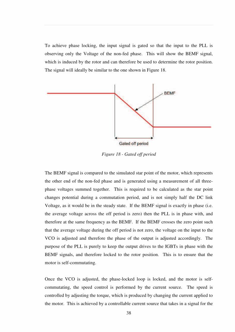
38
To achieve phase locking, the input signal is gated so that the input to the PLL is
observing only the Voltage of the non-fed phase. This will show the BEMF signal,
which is induced by the rotor and can therefore be used to determine the rotor position.
The signal will ideally be similar to the one shown in Figure 18.
Figure 18 - Gated off period
The BEMF signal is compared to the simulated star point of the motor, which represents
the other end of the non-fed phase and is generated using a measurement of all three-
phase voltages summed together. This is required to be calculated as the star point
changes potential during a commutation period, and is not simply half the DC link
Voltage, as it would be in the steady state. If the BEMF signal is exactly in phase (i.e.
the average voltage across the off period is zero) then the PLL is in phase with, and
therefore at the same frequency as the BEMF. If the BEMF crosses the zero point such
that the average voltage during the off period is not zero, the voltage on the input to the
VCO is adjusted and therefore the phase of the output is adjusted accordingly. The
purpose of the PLL is purely to keep the output drives to the IGBTs in phase with the
BEMF signals, and therefore locked to the rotor position. This is to ensure that the
motor is self-commutating.
Once the VCO is adjusted, the phase-locked loop is locked, and the motor is self-
commutating, the speed control is performed by the current source. The speed is
controlled by adjusting the torque, which is produced by changing the current applied to
the motor. This is achieved by a controllable current source that takes in a signal for the
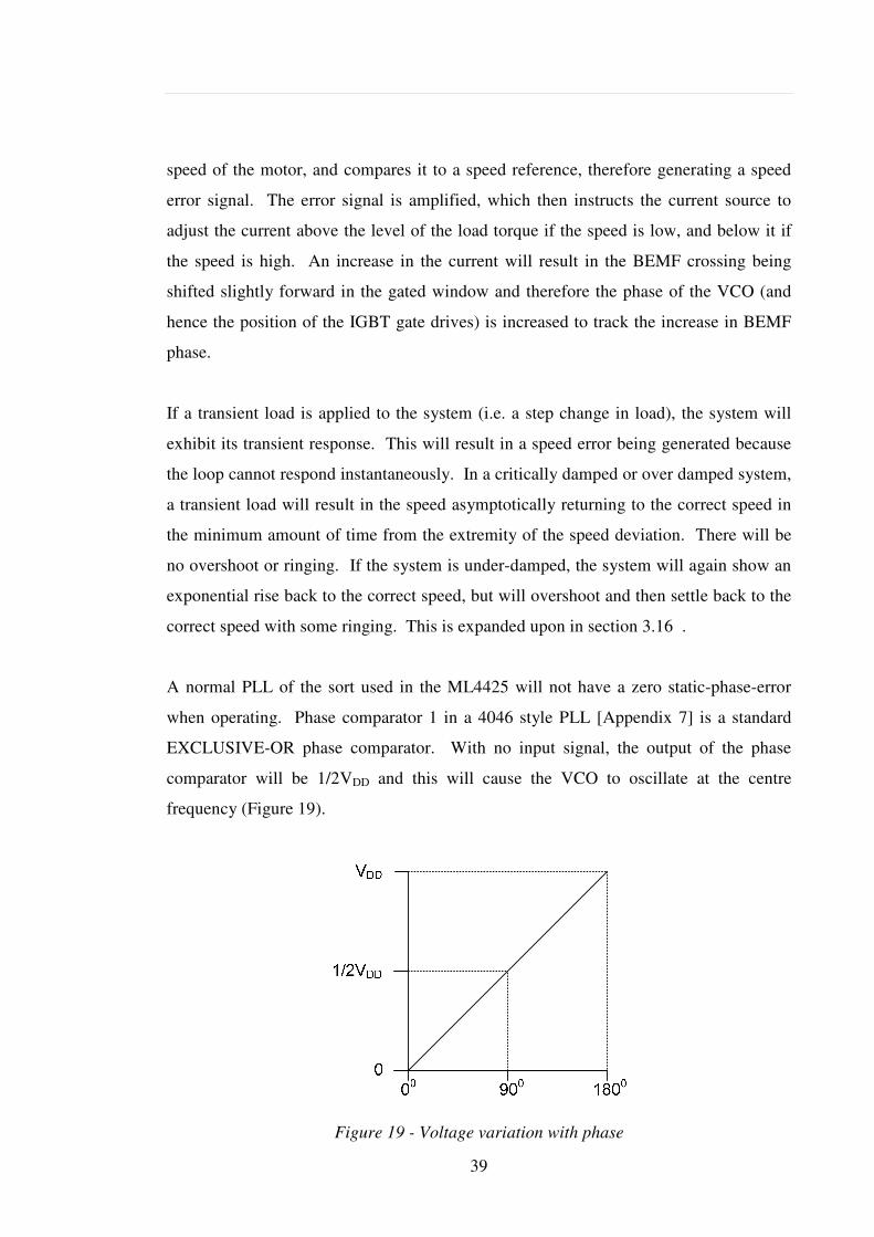
39
speed of the motor, and compares it to a speed reference, therefore generating a speed
error signal. The error signal is amplified, which then instructs the current source to
adjust the current above the level of the load torque if the speed is low, and below it if
the speed is high. An increase in the current will result in the BEMF crossing being
shifted slightly forward in the gated window and therefore the phase of the VCO (and
hence the position of the IGBT gate drives) is increased to track the increase in BEMF
phase.
If a transient load is applied to the system (i.e. a step change in load), the system will
exhibit its transient response. This will result in a speed error being generated because
the loop cannot respond instantaneously. In a critically damped or over damped system,
a transient load will result in the speed asymptotically returning to the correct speed in
the minimum amount of time from the extremity of the speed deviation. There will be
no overshoot or ringing. If the system is under-damped, the system will again show an
exponential rise back to the correct speed, but will overshoot and then settle back to the
correct speed with some ringing. This is expanded upon in section 3.16 .
A normal PLL of the sort used in the ML4425 will not have a zero static-phase-error
when operating. Phase comparator 1 in a 4046 style PLL [Appendix 7] is a standard
EXCLUSIVE-OR phase comparator. With no input signal, the output of the phase
comparator will be 1/2VDD and this will cause the VCO to oscillate at the centre
frequency (Figure 19).
Figure 19 - Voltage variation with phase
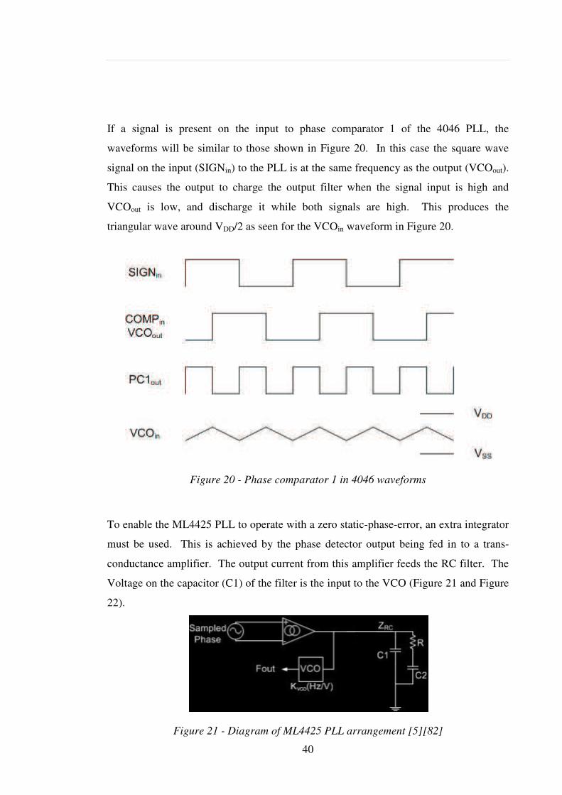
40
If a signal is present on the input to phase comparator 1 of the 4046 PLL, the
waveforms will be similar to those shown in Figure 20. In this case the square wave
signal on the input (SIGNin) to the PLL is at the same frequency as the output (VCOout).
This causes the output to charge the output filter when the signal input is high and
VCOout is low, and discharge it while both signals are high. This produces the
triangular wave around VDD/2 as seen for the VCOin waveform in Figure 20.
Figure 20 - Phase comparator 1 in 4046 waveforms
To enable the ML4425 PLL to operate with a zero static-phase-error, an extra integrator
must be used. This is achieved by the phase detector output being fed in to a trans-
conductance amplifier. The output current from this amplifier feeds the RC filter. The
Voltage on the capacitor (C1) of the filter is the input to the VCO (Figure 21 and Figure
22).
Figure 21 - Diagram of ML4425 PLL arrangement [5][82]
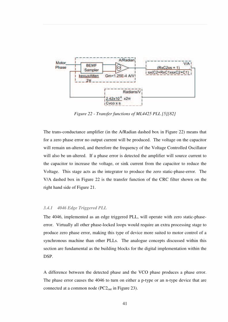
41
Figure 22 - Transfer functions of ML4425 PLL [5][82]
The trans-conductance amplifier (in the A/Radian dashed box in Figure 22) means that
for a zero phase error no output current will be produced. The voltage on the capacitor
will remain un-altered, and therefore the frequency of the Voltage Controlled Oscillator
will also be un-altered. If a phase error is detected the amplifier will source current to
the capacitor to increase the voltage, or sink current from the capacitor to reduce the
Voltage. This stage acts as the integrator to produce the zero static-phase-error. The
V/A dashed box in Figure 22 is the transfer function of the CRC filter shown on the
right hand side of Figure 21.
3.4.1 4046 Edge Triggered PLL
The 4046, implemented as an edge triggered PLL, will operate with zero static-phase-
error. Virtually all other phase-locked loops would require an extra processing stage to
produce zero phase error, making this type of device more suited to motor control of a
synchronous machine than other PLLs. The analogue concepts discussed within this
section are fundamental as the building blocks for the digital implementation within the
DSP.
A difference between the detected phase and the VCO phase produces a phase error.
The phase error causes the 4046 to turn on either a p-type or an n-type device that are
connected at a common node (PC2out in Figure 23).
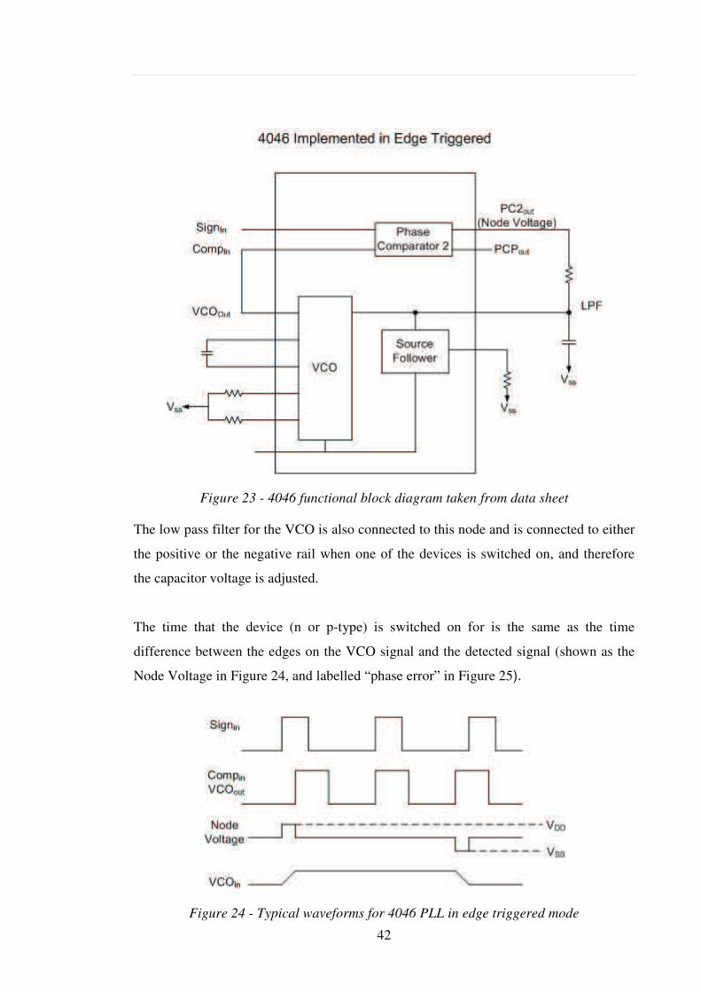
42
Figure 23 - 4046 functional block diagram taken from data sheet
The low pass filter for the VCO is also connected to this node and is connected to either
the positive or the negative rail when one of the devices is switched on, and therefore
the capacitor voltage is adjusted.
The time that the device (n or p-type) is switched on for is the same as the time
difference between the edges on the VCO signal and the detected signal (shown as the
Node Voltage in Figure 24, and labelled “phase error” in Figure 25).
Figure 24 - Typical waveforms for 4046 PLL in edge triggered mode
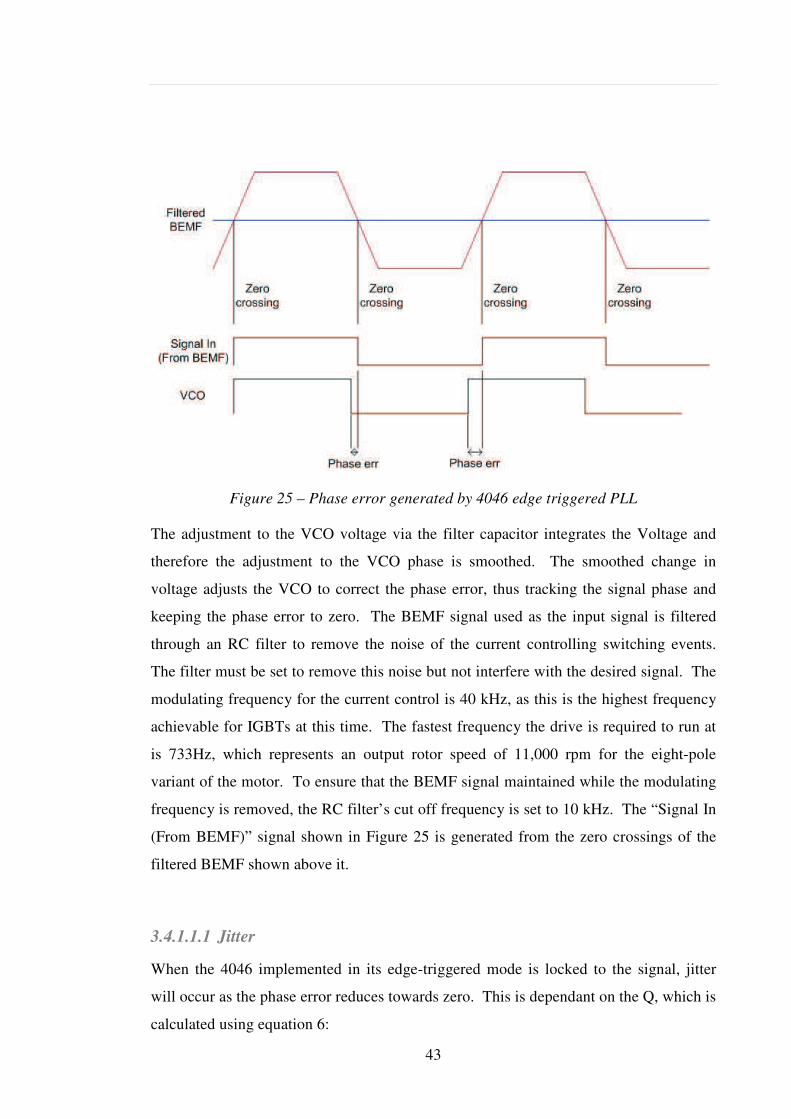
43
Figure 25 – Phase error generated by 4046 edge triggered PLL
The adjustment to the VCO voltage via the filter capacitor integrates the Voltage and
therefore the adjustment to the VCO phase is smoothed. The smoothed change in
voltage adjusts the VCO to correct the phase error, thus tracking the signal phase and
keeping the phase error to zero. The BEMF signal used as the input signal is filtered
through an RC filter to remove the noise of the current controlling switching events.
The filter must be set to remove this noise but not interfere with the desired signal. The
modulating frequency for the current control is 40 kHz, as this is the highest frequency
achievable for IGBTs at this time. The fastest frequency the drive is required to run at
is 733Hz, which represents an output rotor speed of 11,000 rpm for the eight-pole
variant of the motor. To ensure that the BEMF signal maintained while the modulating
frequency is removed, the RC filter’s cut off frequency is set to 10 kHz. The “Signal In
(From BEMF)” signal shown in Figure 25 is generated from the zero crossings of the
filtered BEMF shown above it.
3.4.1.1.1 Jitter
When the 4046 implemented in its edge-triggered mode is locked to the signal, jitter
will occur as the phase error reduces towards zero. This is dependant on the Q, which is
calculated using equation 6:

44
φ∆
Π=
CRKoVccQ (6)
Where Ko is the VCO gain, Vcc is the supply rail to the PLL, C & R are the filter
components on the PLL, and is the amount of jitter. To calculate the values for R
and C, the fastest change in frequency possible must be known, which is calculable by
the fastest acceleration experienced by the motor. This is calculable from the motor
parameters (supplied by Brian Cooper – calculated from the motor design) listed below:
Inertia (J) 2.8e-5 kg.m2
Torque (Te) 1.35 Nm
Fan torque char. (k) 1.017e-6 rad/s2
Viscous Friction (B) 1e-6 Nm.s (estimated)
and have the relationship:
TekBdt
dJ =++ 2ωω
ω (7)
For the steady state situation ( 0=dt
dω), the speed can be calculated using the quadratic
formula (8):
k
kTeBB
2
42 −±−=ω (8)
The stated parameters give = 1151.7 rad/s (equivalent to 11,500 rpm), which is the
correct running speed for the motor.
To calculate the transient characteristics, and hence the maximum acceleration that the
motor can perform (i.e. the fastest frequency change the PLL will have to track) a
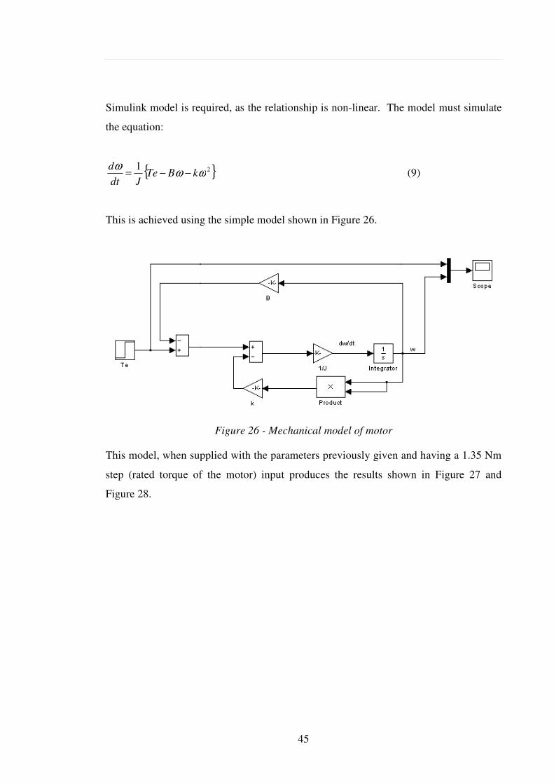
Simulink model is required, as the relationship is
the equation:
1ωω
ωkBTe
Jdt
d−−=
This is achieved using the
This model, when supplied with the parameters previ
step (rated torque of the motor)
Figure 28.
45
Simulink model is required, as the relationship is non-linear. The model must simulate
2ω
This is achieved using the simple model shown in Figure 26.
Figure 26 - Mechanical model of motor
This model, when supplied with the parameters previously given and having a 1.35
(rated torque of the motor) input produces the results shown in
linear. The model must simulate
(9)
ously given and having a 1.35 Nm
input produces the results shown in Figure 27 and
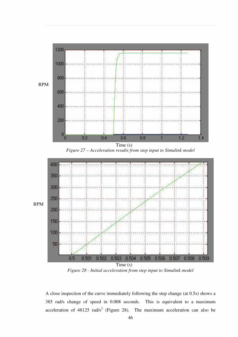
46
Figure 27 – Acceleration results from step input to Simulink model
Figure 28 - Initial acceleration from step input to Simulink model
A close inspection of the curve immediately following the step change (at 0.5s) shows a
385 rad/s change of speed in 0.008 seconds. This is equivalent to a maximum
acceleration of 48125 rad/s2 (Figure 28). The maximum acceleration can also be
RPM
RPM
Time (s)
Time (s)
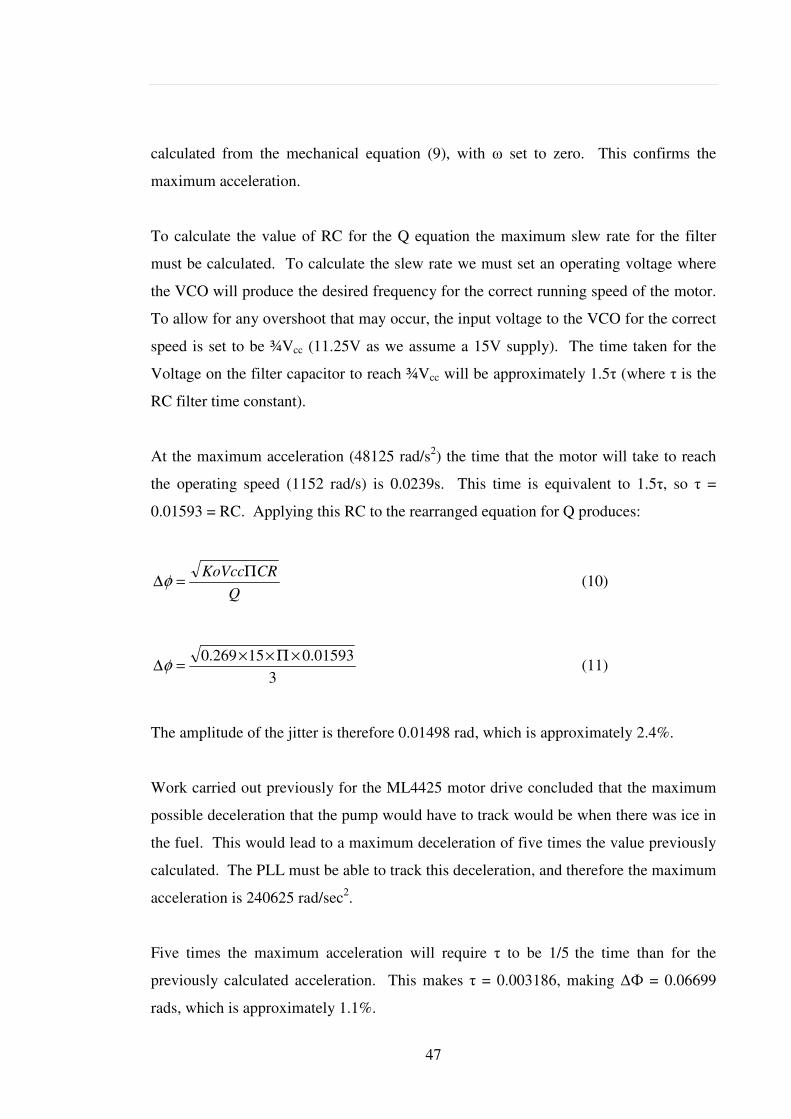
47
calculated from the mechanical equation (9), with set to zero. This confirms the
maximum acceleration.
To calculate the value of RC for the Q equation the maximum slew rate for the filter
must be calculated. To calculate the slew rate we must set an operating voltage where
the VCO will produce the desired frequency for the correct running speed of the motor.
To allow for any overshoot that may occur, the input voltage to the VCO for the correct
speed is set to be ¾Vcc (11.25V as we assume a 15V supply). The time taken for the
Voltage on the filter capacitor to reach ¾Vcc will be approximately 1.5 (where is the
RC filter time constant).
At the maximum acceleration (48125 rad/s2) the time that the motor will take to reach
the operating speed (1152 rad/s) is 0.0239s. This time is equivalent to 1.5, so =
0.01593 = RC. Applying this RC to the rearranged equation for Q produces:
Q
CRKoVccΠ=∆φ (10)
3
01593.015269.0 ×Π××=∆φ (11)
The amplitude of the jitter is therefore 0.01498 rad, which is approximately 2.4%.
Work carried out previously for the ML4425 motor drive concluded that the maximum
possible deceleration that the pump would have to track would be when there was ice in
the fuel. This would lead to a maximum deceleration of five times the value previously
calculated. The PLL must be able to track this deceleration, and therefore the maximum
acceleration is 240625 rad/sec2.
Five times the maximum acceleration will require to be 1/5 the time than for the
previously calculated acceleration. This makes = 0.003186, making = 0.06699
rads, which is approximately 1.1%.

48
The percentage jitter increases as Q increases and decreases, but is within an
acceptable limit.
3.5 DSP Implementation (ML4425 PLL)
To implement a direct copy of the ML4425 PLL the following sequence would be
followed:
1. The rotor will be aligned to a know position by applying full current through
two upper IGBTs and one lower IGBT (Figure 29).
2. The commutation pulses applied with full current in increasing frequency until
the rotor is spinning fast enough that the BEMF is detectable.
3. The input signal will then be gated so that the signal observed by the software at
any one instant is the non-fed phase. The signal is referenced to the virtual star
point, so there is no need to calculate this point in software.
4. The phase observed during each commutation state will be integrated with
respect to the zero crossing value that was read in to the register at the start up of
the drive.
5. If the result of the integrated signal is not zero (i.e. the BEMF signal is not in the
centre of the gated window) then the value produced will be used to adjust the
phase of the commutation pulses. This value must then also be integrated to
produce a smooth transition when a variation in the phase does occur. The filter
must also ensure that the analogue loop is stable. The software must produce an
equivalent response to the RCC filter used in the ML4425 drive to ensure that
the software accurately mimics the analogue response.
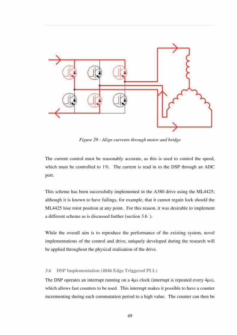
49
Figure 29 - Align currents through motor and bridge
The current control must be reasonably accurate, as this is used to control the speed,
which must be controlled to 1%. The current is read in to the DSP through an ADC
port.
This scheme has been successfully implemented in the A380 drive using the ML4425;
although it is known to have failings, for example, that it cannot regain lock should the
ML4425 lose rotor position at any point. For this reason, it was desirable to implement
a different scheme as is discussed further (section 3.6 ).
While the overall aim is to reproduce the performance of the existing system, novel
implementations of the control and drive, uniquely developed during the research will
be applied throughout the physical realisation of the drive.
3.6 DSP Implementation (4046 Edge Triggered PLL)
The DSP operates an interrupt running on a 4µs clock (interrupt is repeated every 4µs),
which allows fast counters to be used. This interrupt makes it possible to have a counter
incrementing during each commutation period to a high value. The counter can then be
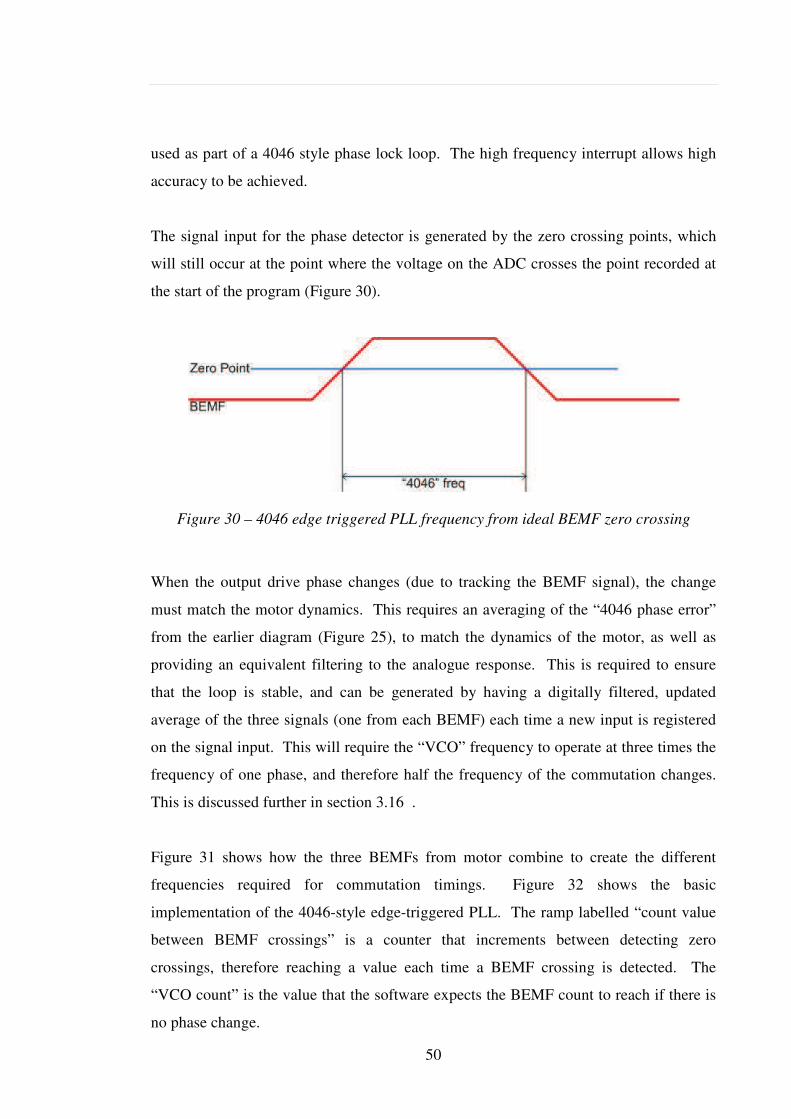
50
used as part of a 4046 style phase lock loop. The high frequency interrupt allows high
accuracy to be achieved.
The signal input for the phase detector is generated by the zero crossing points, which
will still occur at the point where the voltage on the ADC crosses the point recorded at
the start of the program (Figure 30).
Figure 30 – 4046 edge triggered PLL frequency from ideal BEMF zero crossing
When the output drive phase changes (due to tracking the BEMF signal), the change
must match the motor dynamics. This requires an averaging of the “4046 phase error”
from the earlier diagram (Figure 25), to match the dynamics of the motor, as well as
providing an equivalent filtering to the analogue response. This is required to ensure
that the loop is stable, and can be generated by having a digitally filtered, updated
average of the three signals (one from each BEMF) each time a new input is registered
on the signal input. This will require the “VCO” frequency to operate at three times the
frequency of one phase, and therefore half the frequency of the commutation changes.
This is discussed further in section 3.16 .
Figure 31 shows how the three BEMFs from motor combine to create the different
frequencies required for commutation timings. Figure 32 shows the basic
implementation of the 4046-style edge-triggered PLL. The ramp labelled “count value
between BEMF crossings” is a counter that increments between detecting zero
crossings, therefore reaching a value each time a BEMF crossing is detected. The
“VCO count” is the value that the software expects the BEMF count to reach if there is
no phase change.
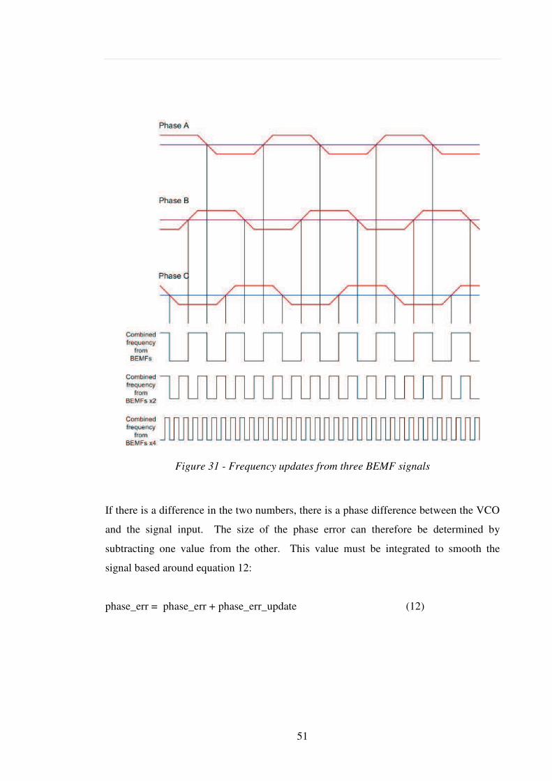
51
Figure 31 - Frequency updates from three BEMF signals
If there is a difference in the two numbers, there is a phase difference between the VCO
and the signal input. The size of the phase error can therefore be determined by
subtracting one value from the other. This value must be integrated to smooth the
signal based around equation 12:
phase_err = phase_err + phase_err_update (12)
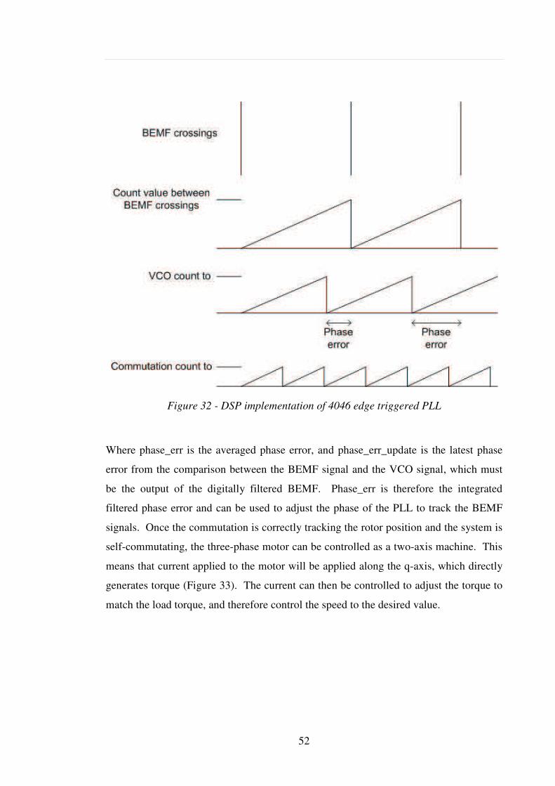
52
Figure 32 - DSP implementation of 4046 edge triggered PLL
Where phase_err is the averaged phase error, and phase_err_update is the latest phase
error from the comparison between the BEMF signal and the VCO signal, which must
be the output of the digitally filtered BEMF. Phase_err is therefore the integrated
filtered phase error and can be used to adjust the phase of the PLL to track the BEMF
signals. Once the commutation is correctly tracking the rotor position and the system is
self-commutating, the three-phase motor can be controlled as a two-axis machine. This
means that current applied to the motor will be applied along the q-axis, which directly
generates torque (Figure 33). The current can then be controlled to adjust the torque to
match the load torque, and therefore control the speed to the desired value.
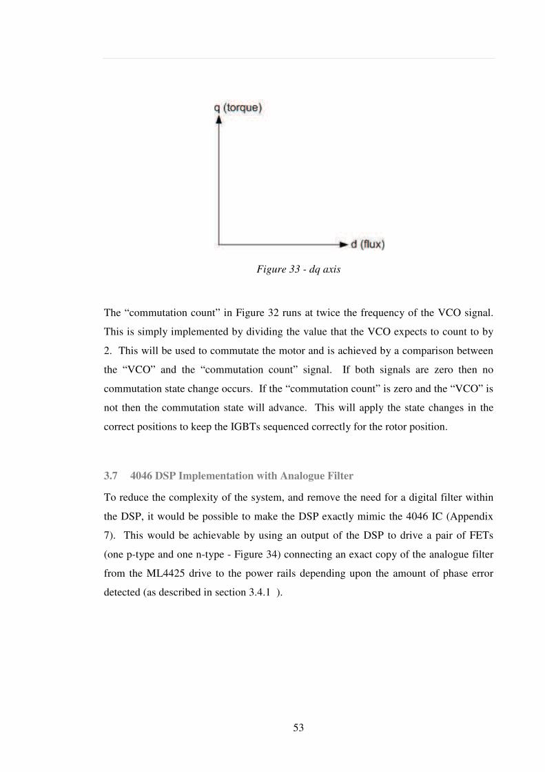
53
Figure 33 - dq axis
The “commutation count” in Figure 32 runs at twice the frequency of the VCO signal.
This is simply implemented by dividing the value that the VCO expects to count to by
2. This will be used to commutate the motor and is achieved by a comparison between
the “VCO” and the “commutation count” signal. If both signals are zero then no
commutation state change occurs. If the “commutation count” is zero and the “VCO” is
not then the commutation state will advance. This will apply the state changes in the
correct positions to keep the IGBTs sequenced correctly for the rotor position.
3.7 4046 DSP Implementation with Analogue Filter
To reduce the complexity of the system, and remove the need for a digital filter within
the DSP, it would be possible to make the DSP exactly mimic the 4046 IC (Appendix
7). This would be achievable by using an output of the DSP to drive a pair of FETs
(one p-type and one n-type - Figure 34) connecting an exact copy of the analogue filter
from the ML4425 drive to the power rails depending upon the amount of phase error
detected (as described in section 3.4.1 ).
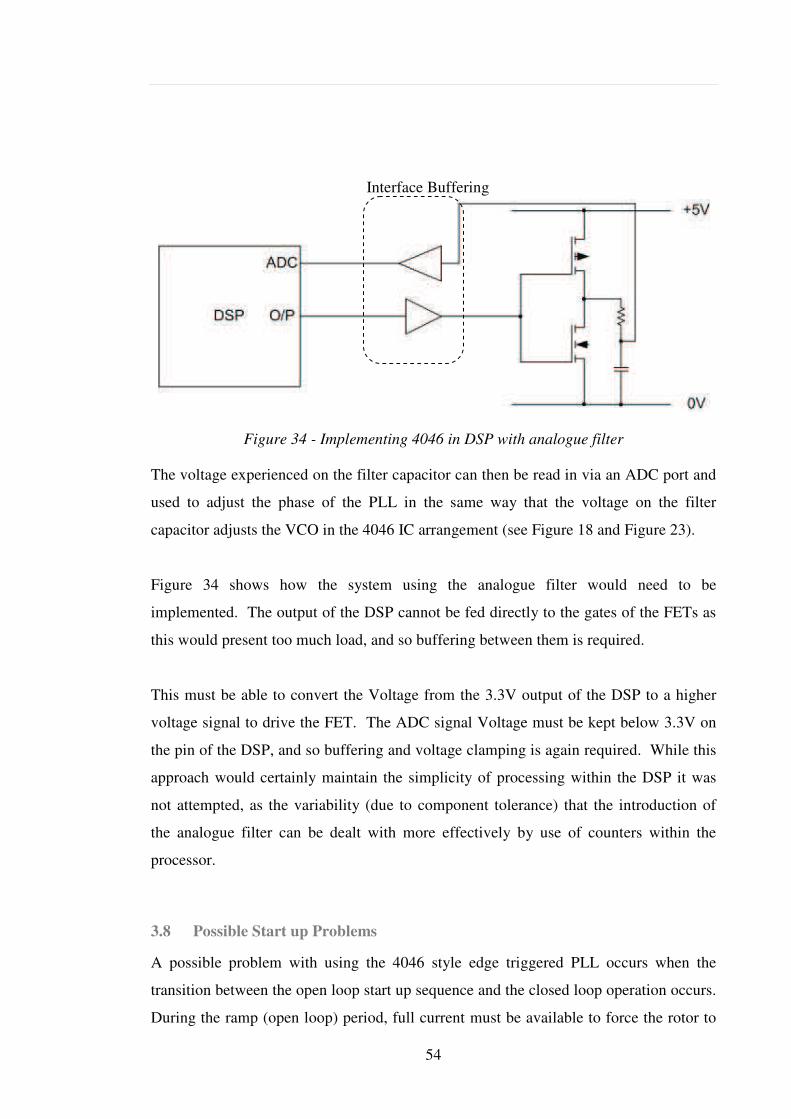
54
Figure 34 - Implementing 4046 in DSP with analogue filter
The voltage experienced on the filter capacitor can then be read in via an ADC port and
used to adjust the phase of the PLL in the same way that the voltage on the filter
capacitor adjusts the VCO in the 4046 IC arrangement (see Figure 18 and Figure 23).
Figure 34 shows how the system using the analogue filter would need to be
implemented. The output of the DSP cannot be fed directly to the gates of the FETs as
this would present too much load, and so buffering between them is required.
This must be able to convert the Voltage from the 3.3V output of the DSP to a higher
voltage signal to drive the FET. The ADC signal Voltage must be kept below 3.3V on
the pin of the DSP, and so buffering and voltage clamping is again required. While this
approach would certainly maintain the simplicity of processing within the DSP it was
not attempted, as the variability (due to component tolerance) that the introduction of
the analogue filter can be dealt with more effectively by use of counters within the
processor.
3.8 Possible Start up Problems
A possible problem with using the 4046 style edge triggered PLL occurs when the
transition between the open loop start up sequence and the closed loop operation occurs.
During the ramp (open loop) period, full current must be available to force the rotor to
Interface Buffering
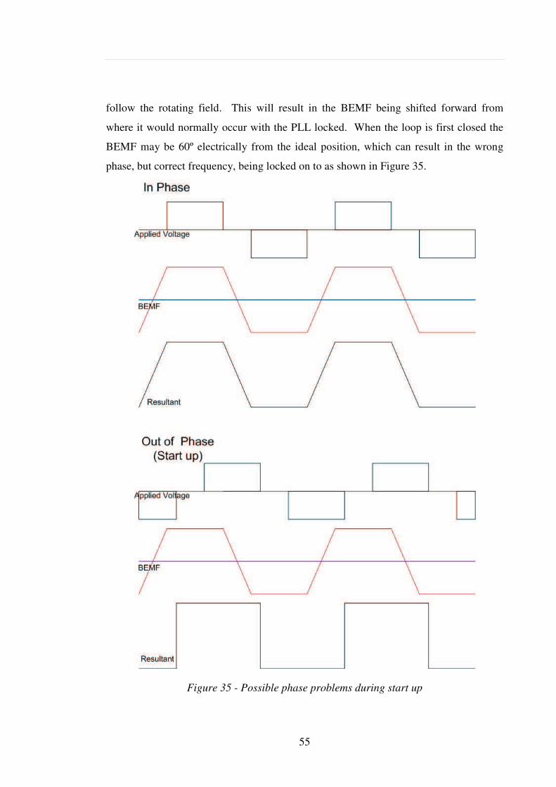
55
follow the rotating field. This will result in the BEMF being shifted forward from
where it would normally occur with the PLL locked. When the loop is first closed the
BEMF may be 60º electrically from the ideal position, which can result in the wrong
phase, but correct frequency, being locked on to as shown in Figure 35.
Figure 35 - Possible phase problems during start up
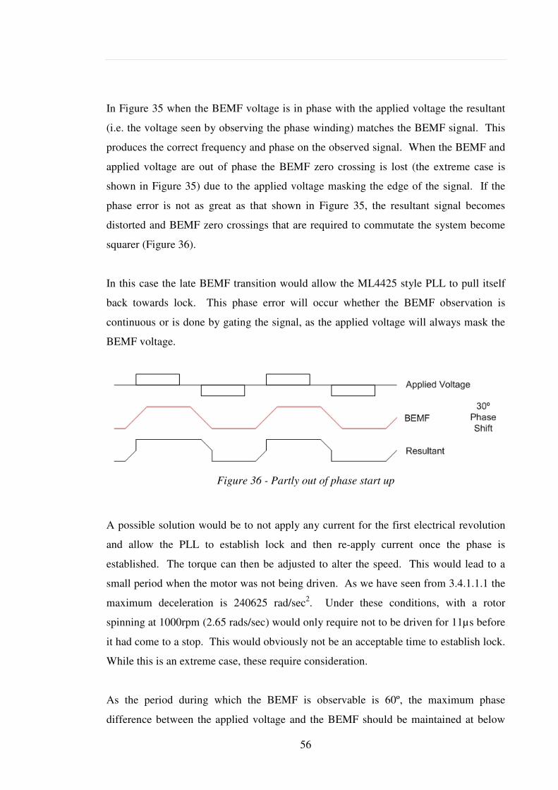
56
In Figure 35 when the BEMF voltage is in phase with the applied voltage the resultant
(i.e. the voltage seen by observing the phase winding) matches the BEMF signal. This
produces the correct frequency and phase on the observed signal. When the BEMF and
applied voltage are out of phase the BEMF zero crossing is lost (the extreme case is
shown in Figure 35) due to the applied voltage masking the edge of the signal. If the
phase error is not as great as that shown in Figure 35, the resultant signal becomes
distorted and BEMF zero crossings that are required to commutate the system become
squarer (Figure 36).
In this case the late BEMF transition would allow the ML4425 style PLL to pull itself
back towards lock. This phase error will occur whether the BEMF observation is
continuous or is done by gating the signal, as the applied voltage will always mask the
BEMF voltage.
Figure 36 - Partly out of phase start up
A possible solution would be to not apply any current for the first electrical revolution
and allow the PLL to establish lock and then re-apply current once the phase is
established. The torque can then be adjusted to alter the speed. This would lead to a
small period when the motor was not being driven. As we have seen from 3.4.1.1.1 the
maximum deceleration is 240625 rad/sec2. Under these conditions, with a rotor
spinning at 1000rpm (2.65 rads/sec) would only require not to be driven for 11µs before
it had come to a stop. This would obviously not be an acceptable time to establish lock.
While this is an extreme case, these require consideration.
As the period during which the BEMF is observable is 60º, the maximum phase
difference between the applied voltage and the BEMF should be maintained at below

57
40º to ensure that there is enough of the BEMF signal present during the non-fed phase,
where there is no voltage applied to the motor, to ensure the signal can be successfully
locked on to.
3.9 Digitally matching the analogue filter response
The analogue filter used in the control loop of the ML4425 drive (shown in Figure 21)
consists of an RCC arrangement, with one capacitor in parallel with a series RC. This
produces the s-domain transfer function:
)(
1
1212
2
CsCRCCs
sRC
++
+ (13)
To match the motor dynamics and ensure that the loop is stable, the capacitor and
resistor values on the ML4425 drive were chosen to be:
R 14k3
C1 15nF
C2 100nF
These values were arrived at during the initial simulation work previously undertaken
by Eaton at the start of the programme.
Using these component values, the analogue response is known. To calculate the digital
response a series of equations must be used to determine the coefficients that can then
be used in a structure as shown in Figure 37 [83].

58
Figure 37 - Digital IIR filter implementation
The transfer function for the system in the z-domain is:
−−
++−−
−−
21
21
1
1
bZaZ
BZAZm (14)
The structure show in Figure 37 was to be used to be used to replicate the analogue
filter used on the PLL of the ML4425. However, the only useful information required
from the PLL and its filter is the maximum rate of change in frequency of the motor that
it can track. The specification for this was defined and is analysed in section 3.16 .
3.10 Motor Characteristics
There are three different motors used in the A380 pump types. These are the feed, trim,
and transfer. The feed motor operates at 11,500 rpm, the transfer at 8850 rpm, and the
trim at 8500 rpm. Each motor is a six pole BLDC, therefore making the commutation
frequency of the square wave output drive three times the motor speed, as there are
three electrical revolutions per mechanical revolution of the shaft. The development
process for the motor design was in conjunction with a part DTI funded program known
as CARAD Times which produced the experimental test facility shown in Figure 38.
The rig developed for this program used a modified A320 pump (originally a three-
phase induction motor) replaced by an eight pole Brushless DC motor. The rig and
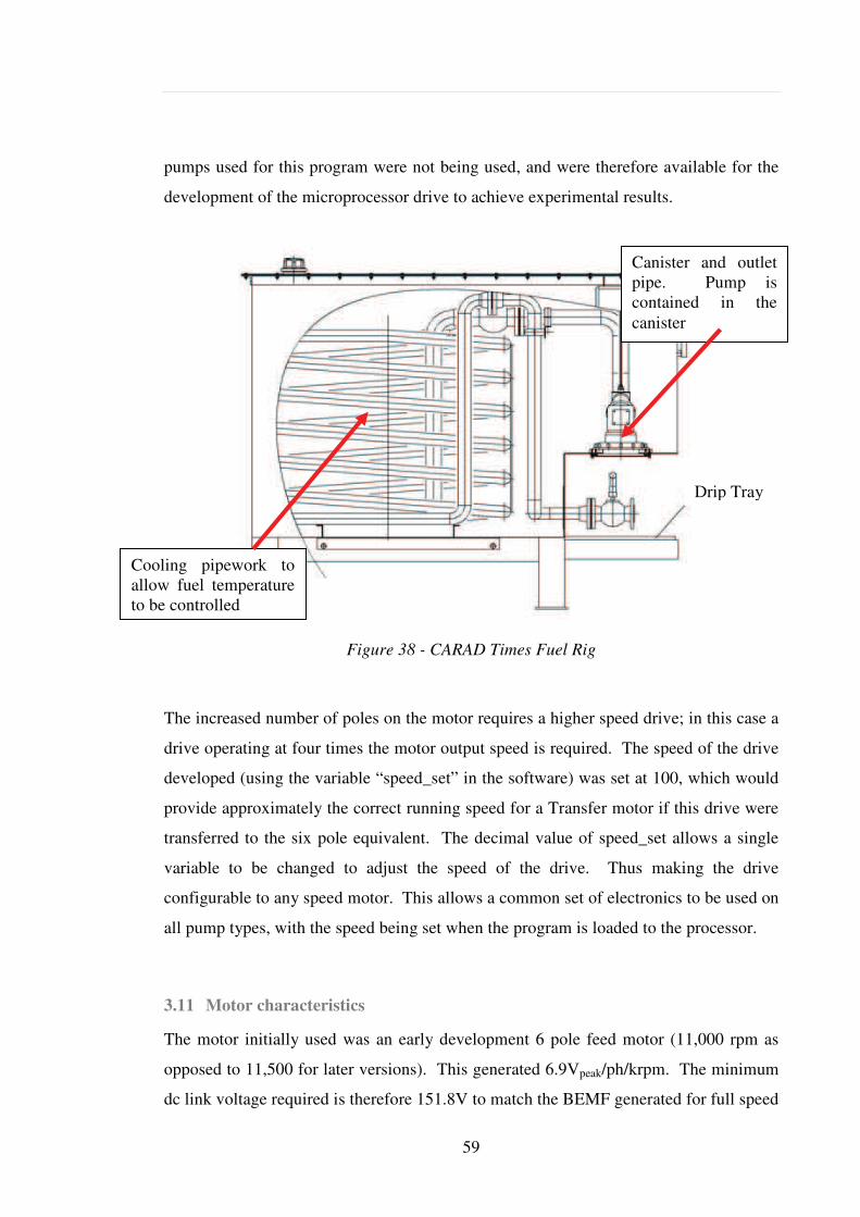
59
pumps used for this program were not being used, and were therefore available for the
development of the microprocessor drive to achieve experimental results.
Figure 38 - CARAD Times Fuel Rig
The increased number of poles on the motor requires a higher speed drive; in this case a
drive operating at four times the motor output speed is required. The speed of the drive
developed (using the variable “speed_set” in the software) was set at 100, which would
provide approximately the correct running speed for a Transfer motor if this drive were
transferred to the six pole equivalent. The decimal value of speed_set allows a single
variable to be changed to adjust the speed of the drive. Thus making the drive
configurable to any speed motor. This allows a common set of electronics to be used on
all pump types, with the speed being set when the program is loaded to the processor.
3.11 Motor characteristics
The motor initially used was an early development 6 pole feed motor (11,000 rpm as
opposed to 11,500 for later versions). This generated 6.9Vpeak/ph/krpm. The minimum
dc link voltage required is therefore 151.8V to match the BEMF generated for full speed
Canister and outlet pipe. Pump is contained in the
canister
Drip Tray
Cooling pipework to allow fuel temperature to be controlled
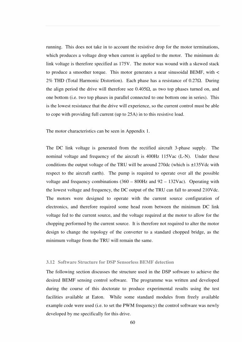
60
running. This does not take in to account the resistive drop for the motor terminations,
which produces a voltage drop when current is applied to the motor. The minimum dc
link voltage is therefore specified as 175V. The motor was wound with a skewed stack
to produce a smoother torque. This motor generates a near sinusoidal BEMF, with <
2% THD (Total Harmonic Distortion). Each phase has a resistance of 0.27. During
the align period the drive will therefore see 0.405, as two top phases turned on, and
one bottom (i.e. two top phases in parallel connected to one bottom one in series). This
is the lowest resistance that the drive will experience, so the current control must be able
to cope with providing full current (up to 25A) in to this resistive load.
The motor characteristics can be seen in Appendix 1.
The DC link voltage is generated from the rectified aircraft 3-phase supply. The
nominal voltage and frequency of the aircraft is 400Hz 115Vac (L-N). Under these
conditions the output voltage of the TRU will be around 270dc (which is ±135Vdc with
respect to the aircraft earth). The pump is required to operate over all the possible
voltage and frequency combinations (360 – 800Hz and 92 – 132Vac). Operating with
the lowest voltage and frequency, the DC output of the TRU can fall to around 210Vdc.
The motors were designed to operate with the current source configuration of
electronics, and therefore required some head room between the minimum DC link
voltage fed to the current source, and the voltage required at the motor to allow for the
chopping performed by the current source. It is therefore not required to alter the motor
design to change the topology of the converter to a standard chopped bridge, as the
minimum voltage from the TRU will remain the same.
3.12 Software Structure for DSP Sensorless BEMF detection
The following section discusses the structure used in the DSP software to achieve the
desired BEMF sensing control software. The programme was written and developed
during the course of this doctorate to produce experimental results using the test
facilities available at Eaton. While some standard modules from freely available
example code were used (i.e. to set the PWM frequency) the control software was newly
developed by me specifically for this drive.
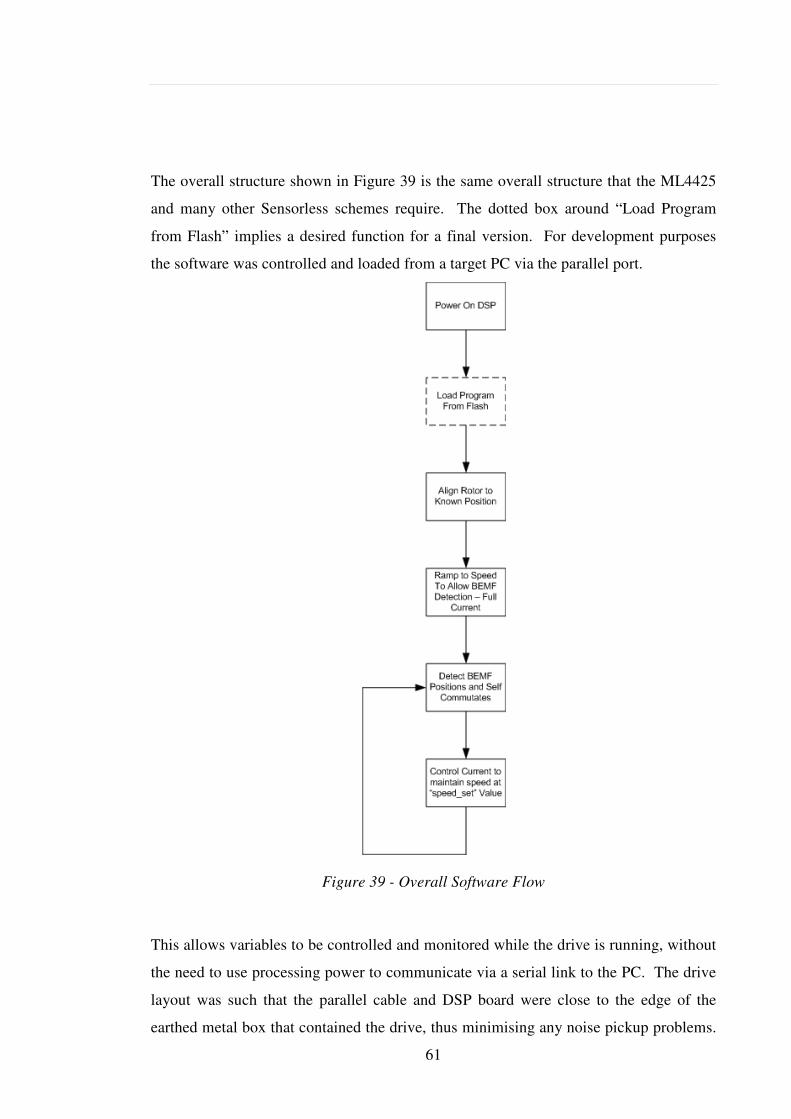
61
The overall structure shown in Figure 39 is the same overall structure that the ML4425
and many other Sensorless schemes require. The dotted box around “Load Program
from Flash” implies a desired function for a final version. For development purposes
the software was controlled and loaded from a target PC via the parallel port.
Figure 39 - Overall Software Flow
This allows variables to be controlled and monitored while the drive is running, without
the need to use processing power to communicate via a serial link to the PC. The drive
layout was such that the parallel cable and DSP board were close to the edge of the
earthed metal box that contained the drive, thus minimising any noise pickup problems.

62
Using a separate DC supply to the motor bridge also helped reduce the noise content of
the local ground.
3.13 Commutation Software Structure
The commutation of the motor phases is applied using software within the DSP. This is
controlled (when closed loop) by the BEMF detections fed back to provide rotor
position information. The initial commutation event is the align pulse.
3.13.1 Align
This requires two top and one bottom IGBT to be switched on (Figure 40). This will
move the rotor to a known position, which will be halfway between two commutation
states. In a two pole motor this would result in the rotor being aligned to one of the
windings as shown (Figure 41).
Figure 40 - Align currents in motor bridge
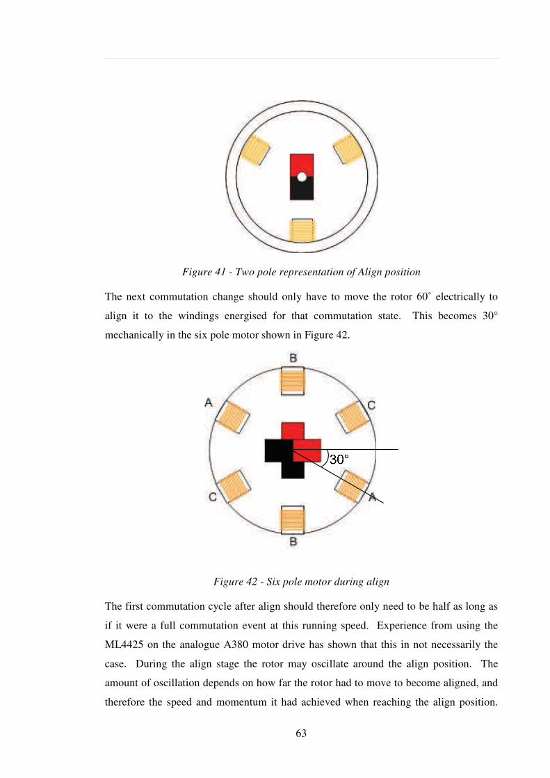
63
Figure 41 - Two pole representation of Align position
The next commutation change should only have to move the rotor 60˚ electrically to
align it to the windings energised for that commutation state. This becomes 30°
mechanically in the six pole motor shown in Figure 42.
Figure 42 - Six pole motor during align
The first commutation cycle after align should therefore only need to be half as long as
if it were a full commutation event at this running speed. Experience from using the
ML4425 on the analogue A380 motor drive has shown that this in not necessarily the
case. During the align stage the rotor may oscillate around the align position. The
amount of oscillation depends on how far the rotor had to move to become aligned, and
therefore the speed and momentum it had achieved when reaching the align position.
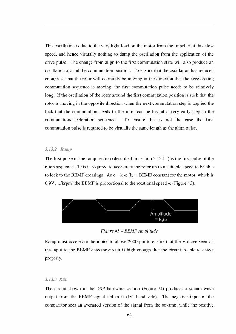
This oscillation is due to the very light load on t
speed, and hence virtually
drive pulse. The change from align to the first co
oscillation around the commutation position. To en
enough so that the rotor will definitely be moving
commutation sequence is moving, the first commutati
long. If the oscillation of the rotor around the f
rotor is moving in the opposite direction whe
lock that the commutation needs to the rotor can be
commutation/acceleration sequence. To ensure this
commutation pulse is
3.13.2 Ramp
The first pulse of the ramp section (described in
ramp sequence. This is required to accelerate the
to lock to the BEMF crossings. As e = k
6.9Vpeak/krpm) the BEMF is proportional to the rotational s
Ramp must accelerate the motor t
the input to the BEMF detector circuit is high enou
properly.
3.13.3 Run
The circuit shown in the DSP hardware section (
output from the BEMF signal fed to it (left hand si
comparator sees an averaged version of the signal f
64
This oscillation is due to the very light load on the motor from the impeller at this slow
virtually nothing to damp the oscillation from
drive pulse. The change from align to the first commutation state will also produce an
oscillation around the commutation position. To ensure that the oscillation has reduced
enough so that the rotor will definitely be moving in the direction that the accelerating
commutation sequence is moving, the first commutation pulse needs to be relatively
long. If the oscillation of the rotor around the first commutation position is such that the
rotor is moving in the opposite direction when the next commutation step is applied the
lock that the commutation needs to the rotor can be lost at a very early step in the
commutation/acceleration sequence. To ensure this is not the case the first
commutation pulse is required to be virtually the same length as the align pulse.
The first pulse of the ramp section (described in section 3.13.1 ) is the first pulse of the
ramp sequence. This is required to accelerate the rotor up to a suitable speed to
to lock to the BEMF crossings. As e = ke (ke = BEMF constant for the motor, which is
/krpm) the BEMF is proportional to the rotational speed
Figure 43 – BEMF Amplitude
Ramp must accelerate the motor to above 2000rpm to ensure that the Voltage seen on
the input to the BEMF detector circuit is high enough that the circuit is able to detect
The circuit shown in the DSP hardware section (Figure 74) produces a square wave
output from the BEMF signal fed to it (left hand side). The negative input of the
comparator sees an averaged version of the signal from the op-amp, while the positive
he motor from the impeller at this slow
nothing to damp the oscillation from the application of the
mmutation state will also produce an
sure that the oscillation has reduced
e direction that the accelerating
on pulse needs to be relatively
irst commutation position is such that the
n the next commutation step is applied the
lost at a very early step in the
is not the case the first
ame length as the align pulse.
) is the first pulse of the
rotor up to a suitable speed to be able
= BEMF constant for the motor, which is
peed (Figure 43).
to ensure that the Voltage seen on
gh that the circuit is able to detect
produces a square wave
de). The negative input of the
amp, while the positive
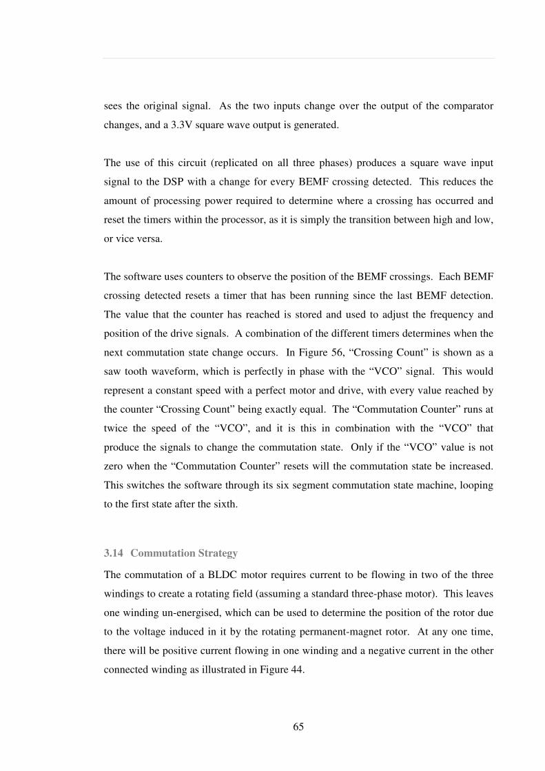
65
sees the original signal. As the two inputs change over the output of the comparator
changes, and a 3.3V square wave output is generated.
The use of this circuit (replicated on all three phases) produces a square wave input
signal to the DSP with a change for every BEMF crossing detected. This reduces the
amount of processing power required to determine where a crossing has occurred and
reset the timers within the processor, as it is simply the transition between high and low,
or vice versa.
The software uses counters to observe the position of the BEMF crossings. Each BEMF
crossing detected resets a timer that has been running since the last BEMF detection.
The value that the counter has reached is stored and used to adjust the frequency and
position of the drive signals. A combination of the different timers determines when the
next commutation state change occurs. In Figure 56, “Crossing Count” is shown as a
saw tooth waveform, which is perfectly in phase with the “VCO” signal. This would
represent a constant speed with a perfect motor and drive, with every value reached by
the counter “Crossing Count” being exactly equal. The “Commutation Counter” runs at
twice the speed of the “VCO”, and it is this in combination with the “VCO” that
produce the signals to change the commutation state. Only if the “VCO” value is not
zero when the “Commutation Counter” resets will the commutation state be increased.
This switches the software through its six segment commutation state machine, looping
to the first state after the sixth.
3.14 Commutation Strategy
The commutation of a BLDC motor requires current to be flowing in two of the three
windings to create a rotating field (assuming a standard three-phase motor). This leaves
one winding un-energised, which can be used to determine the position of the rotor due
to the voltage induced in it by the rotating permanent-magnet rotor. At any one time,
there will be positive current flowing in one winding and a negative current in the other
connected winding as illustrated in Figure 44.
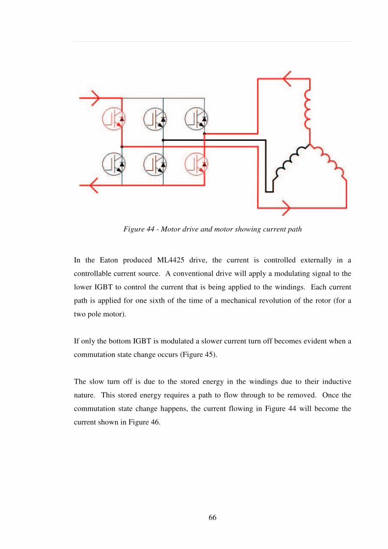
66
Figure 44 - Motor drive and motor showing current path
In the Eaton produced ML4425 drive, the current is controlled externally in a
controllable current source. A conventional drive will apply a modulating signal to the
lower IGBT to control the current that is being applied to the windings. Each current
path is applied for one sixth of the time of a mechanical revolution of the rotor (for a
two pole motor).
If only the bottom IGBT is modulated a slower current turn off becomes evident when a
commutation state change occurs (Figure 45).
The slow turn off is due to the stored energy in the windings due to their inductive
nature. This stored energy requires a path to flow through to be removed. Once the
commutation state change happens, the current flowing in Figure 44 will become the
current shown in Figure 46.
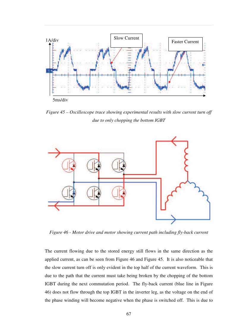
67
Figure 45 – Oscilloscope trace showing experimental results with slow current turn off
due to only chopping the bottom IGBT
Figure 46 - Motor drive and motor showing current path including fly-back current
The current flowing due to the stored energy still flows in the same direction as the
applied current, as can be seen from Figure 46 and Figure 45. It is also noticeable that
the slow current turn off is only evident in the top half of the current waveform. This is
due to the path that the current must take being broken by the chopping of the bottom
IGBT during the next commutation period. The fly-back current (blue line in Figure
46) does not flow through the top IGBT in the inverter leg, as the voltage on the end of
the phase winding will become negative when the phase is switched off. This is due to
Slow Current Faster Current
5ms/div
1A/div
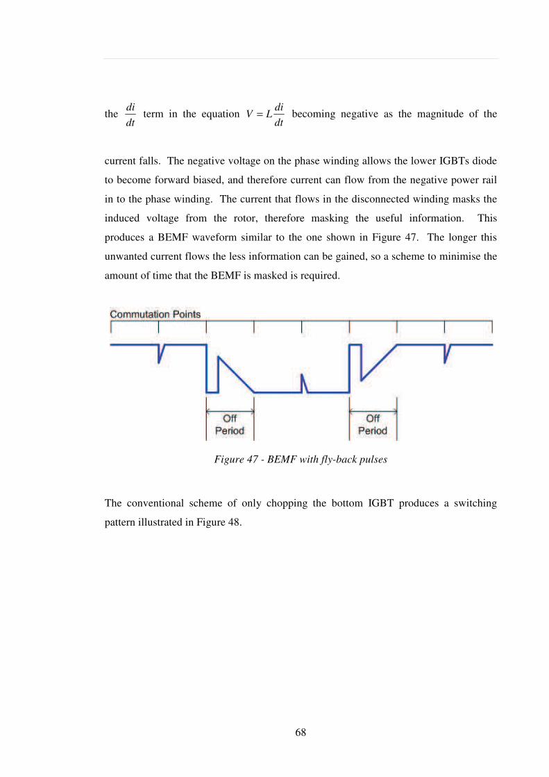
68
the dt
di term in the equation
dt
diLV = becoming negative as the magnitude of the
current falls. The negative voltage on the phase winding allows the lower IGBTs diode
to become forward biased, and therefore current can flow from the negative power rail
in to the phase winding. The current that flows in the disconnected winding masks the
induced voltage from the rotor, therefore masking the useful information. This
produces a BEMF waveform similar to the one shown in Figure 47. The longer this
unwanted current flows the less information can be gained, so a scheme to minimise the
amount of time that the BEMF is masked is required.
Figure 47 - BEMF with fly-back pulses
The conventional scheme of only chopping the bottom IGBT produces a switching
pattern illustrated in Figure 48.
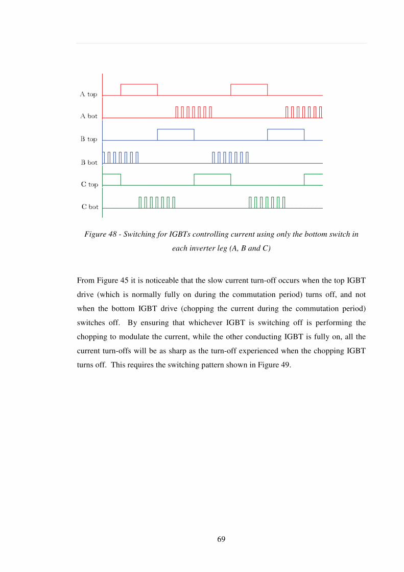
Figure 48 - Switching for IGBTs controlling current using only t
From Figure 45 it is noticeable that the slow current turn
drive (which is normally fully on during the commut
when the bottom IGBT drive (chopping the current du
switches off. By ensuring that whichever IGBT is s
chopping to modulate the current, while the other c
current turn-offs will be as sharp as the turn
turns off. This requires the switching pattern sho
69
witching for IGBTs controlling current using only t
each inverter leg (A, B and C)
it is noticeable that the slow current turn-off occurs when the top IGBT
drive (which is normally fully on during the commutation period) turns off, and
when the bottom IGBT drive (chopping the current during the commutation period)
switches off. By ensuring that whichever IGBT is switching off is performing the
chopping to modulate the current, while the other conducting IGBT is fully on, all the
offs will be as sharp as the turn-off experienced when the chopping IGBT
turns off. This requires the switching pattern shown in Figure 49.
witching for IGBTs controlling current using only the bottom switch in
off occurs when the top IGBT
ation period) turns off, and not
ring the commutation period)
witching off is performing the
onducting IGBT is fully on, all the
off experienced when the chopping IGBT
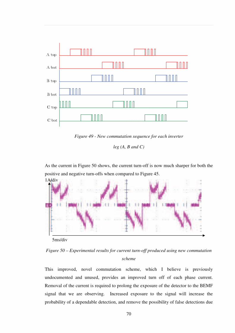
70
Figure 49 - New commutation sequence for each inverter
leg (A, B and C)
As the current in Figure 50 shows, the current turn-off is now much sharper for both the
positive and negative turn-offs when compared to Figure 45.
Figure 50 – Experimental results for current turn-off produced using new commutation
scheme
This improved, novel commutation scheme, which I believe is previously
undocumented and unused, provides an improved turn off of each phase current.
Removal of the current is required to prolong the exposure of the detector to the BEMF
signal that we are observing. Increased exposure to the signal will increase the
probability of a dependable detection, and remove the possibility of false detections due
5ms/div
1A/div
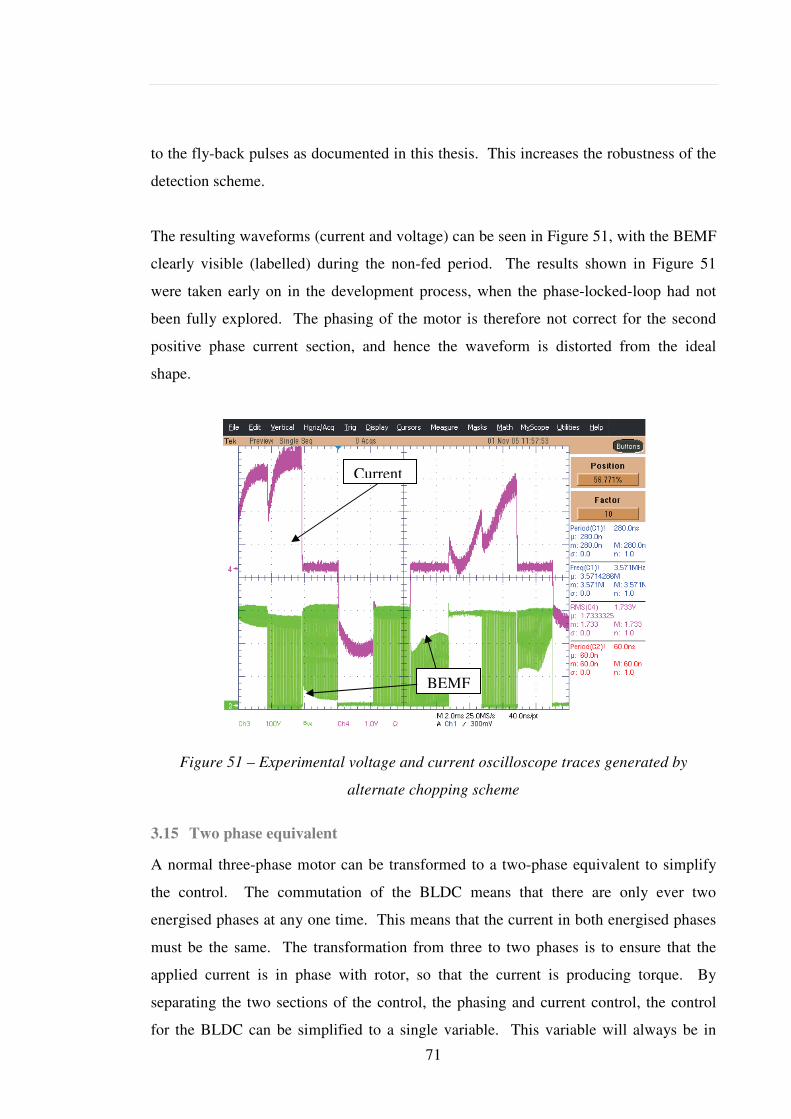
71
to the fly-back pulses as documented in this thesis. This increases the robustness of the
detection scheme.
The resulting waveforms (current and voltage) can be seen in Figure 51, with the BEMF
clearly visible (labelled) during the non-fed period. The results shown in Figure 51
were taken early on in the development process, when the phase-locked-loop had not
been fully explored. The phasing of the motor is therefore not correct for the second
positive phase current section, and hence the waveform is distorted from the ideal
shape.
Figure 51 – Experimental voltage and current oscilloscope traces generated by
alternate chopping scheme
3.15 Two phase equivalent
A normal three-phase motor can be transformed to a two-phase equivalent to simplify
the control. The commutation of the BLDC means that there are only ever two
energised phases at any one time. This means that the current in both energised phases
must be the same. The transformation from three to two phases is to ensure that the
applied current is in phase with rotor, so that the current is producing torque. By
separating the two sections of the control, the phasing and current control, the control
for the BLDC can be simplified to a single variable. This variable will always be in
BEMF
Current
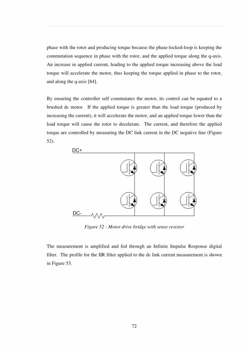
72
phase with the rotor and producing torque because the phase-locked-loop is keeping the
commutation sequence in phase with the rotor, and the applied torque along the q-axis.
An increase in applied current, leading to the applied torque increasing above the load
torque will accelerate the motor, thus keeping the torque applied in phase to the rotor,
and along the q-axis [84].
By ensuring the controller self commutates the motor, its control can be equated to a
brushed dc motor. If the applied torque is greater than the load torque (produced by
increasing the current), it will accelerate the motor, and an applied torque lower than the
load torque will cause the rotor to decelerate. The current, and therefore the applied
torque are controlled by measuring the DC link current in the DC negative line (Figure
52).
Figure 52 - Motor drive bridge with sense resistor
The measurement is amplified and fed through an Infinite Impulse Response digital
filter. The profile for the IIR filter applied to the dc link current measurement is shown
in Figure 53.
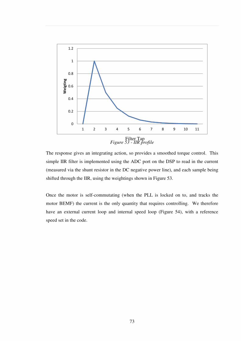
73
Figure 53 - IIR profile
The response gives an integrating action, so provides a smoothed torque control. This
simple IIR filter is implemented using the ADC port on the DSP to read in the current
(measured via the shunt resistor in the DC negative power line), and each sample being
shifted through the IIR, using the weightings shown in Figure 53.
Once the motor is self-commutating (when the PLL is locked on to, and tracks the
motor BEMF) the current is the only quantity that requires controlling. We therefore
have an external current loop and internal speed loop (Figure 54), with a reference
speed set in the code.
Filter Tap
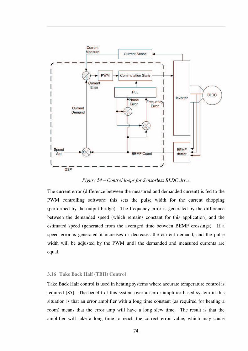
74
Figure 54 – Control loops for Sensorless BLDC drive
The current error (difference between the measured and demanded current) is fed to the
PWM controlling software; this sets the pulse width for the current chopping
(performed by the output bridge). The frequency error is generated by the difference
between the demanded speed (which remains constant for this application) and the
estimated speed (generated from the averaged time between BEMF crossings). If a
speed error is generated it increases or decreases the current demand, and the pulse
width will be adjusted by the PWM until the demanded and measured currents are
equal.
3.16 Take Back Half (TBH) Control
Take Back Half control is used in heating systems where accurate temperature control is
required [85]. The benefit of this system over an error amplifier based system in this
situation is that an error amplifier with a long time constant (as required for heating a
room) means that the error amp will have a long slew time. The result is that the
amplifier will take a long time to reach the correct error value, which may cause
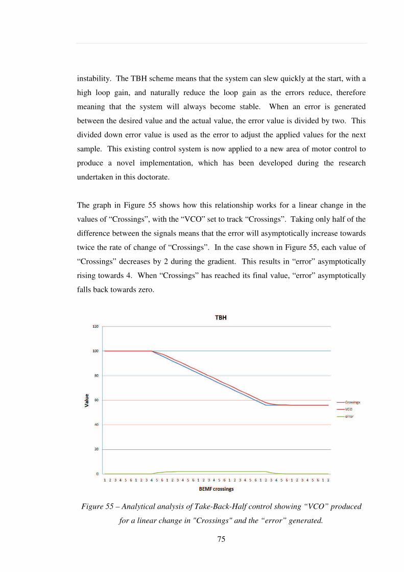
75
instability. The TBH scheme means that the system can slew quickly at the start, with a
high loop gain, and naturally reduce the loop gain as the errors reduce, therefore
meaning that the system will always become stable. When an error is generated
between the desired value and the actual value, the error value is divided by two. This
divided down error value is used as the error to adjust the applied values for the next
sample. This existing control system is now applied to a new area of motor control to
produce a novel implementation, which has been developed during the research
undertaken in this doctorate.
The graph in Figure 55 shows how this relationship works for a linear change in the
values of “Crossings”, with the “VCO” set to track “Crossings”. Taking only half of the
difference between the signals means that the error will asymptotically increase towards
twice the rate of change of “Crossings”. In the case shown in Figure 55, each value of
“Crossings” decreases by 2 during the gradient. This results in “error” asymptotically
rising towards 4. When “Crossings” has reached its final value, “error” asymptotically
falls back towards zero.
Figure 55 – Analytical analysis of Take-Back-Half control showing “VCO” produced
for a linear change in "Crossings" and the “error” generated.
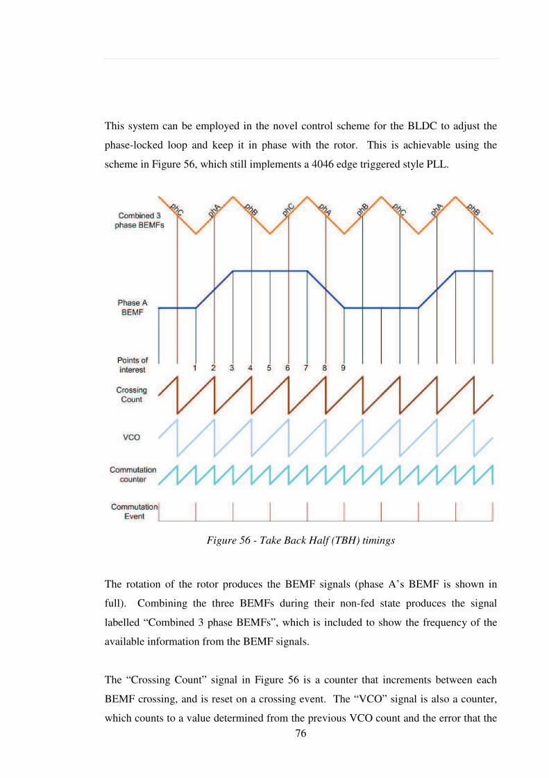
76
This system can be employed in the novel control scheme for the BLDC to adjust the
phase-locked loop and keep it in phase with the rotor. This is achievable using the
scheme in Figure 56, which still implements a 4046 edge triggered style PLL.
Figure 56 - Take Back Half (TBH) timings
The rotation of the rotor produces the BEMF signals (phase A’s BEMF is shown in
full). Combining the three BEMFs during their non-fed state produces the signal
labelled “Combined 3 phase BEMFs”, which is included to show the frequency of the
available information from the BEMF signals.
The “Crossing Count” signal in Figure 56 is a counter that increments between each
BEMF crossing, and is reset on a crossing event. The “VCO” signal is also a counter,
which counts to a value determined from the previous VCO count and the error that the

77
previous VCO count generated. The value that the VCO will count to is calculated by
the difference in value reached on the “Crossing Count” and the “VCO” count divided
by two.
When the error generated between the two signals is zero, the rotor (which generates the
crossing count signal) and VCO are in phase. To commutate the motor correctly, the
commutation events (shown in Figure 56) occur when “Commutation counter” reaches
its “count-to” value (which is half of the value that the “VCO” counts to) and the VCO
is not at its “count-to” value. This requires that the “Commutation Counter” runs at
twice the frequency of the “VCO”, and only produce a commutation event on alternate
counts.
If the rotor changes speed (i.e. due to a change in load torque) an error will be generated
between the detected zero crossings (“Crossing Count”) and the “VCO”. This will also
cause a speed error, which will be used to adjust the current fed to the motor, and
therefore the torque. During this deviation from the desired speed, the VCO will adjust
the phase-locked loop to track the rotor position and keep the motor self-commutating.
The current can then be adjusted to bring the rotor back to the correct operating speed
and balance the load torque.
The “Points of interest” labelled in Figure 56 are:
1. Commutation event occurs when “Commutation Counter” reaches its maximum
value but “VCO” does not, making Phase A the non-fed phase.
2. Zero crossing of phase A’s BEMF is detected, stopping the “Crossing Count”
counter. This value is then compared to the “VCO” value to generate an error, if
the values are not the same.
3. Commutation event occurs when “Commutation Counter” reaches its maximum
value but “VCO” does not, making Phase B the non-fed phase.
4. Zero crossing of phase B’s BEMF is detected, stopping the “Crossing Count”
counter. This value is then compared to the “VCO” value to generate an error, if
the values are not the same.

78
5. A commutation event occurs when “Commutation Counter” reaches its
maximum value but “VCO” does not, making Phase C the non-fed phase.
6. Zero crossing of phase C’s BEMF is detected, stopping the “Crossing Count”
counter. This value is then compared to the “VCO” value to generate an error, if
the values are not the same.
7. Commutation event occurs when “Commutation Counter” reaches its maximum
value but “VCO” does not, making Phase A the non-fed phase again.
8. Zero crossing of phase A’s BEMF is again detected, but has the opposite
gradient to before, stopping the “Crossing Count” counter. This value is then
compared to the “VCO” value to generate an error, if the values are not the
same.
9. Commutation event occurs when “Commutation Counter” reaches its maximum
value but “VCO” does not, making Phase B the non-fed phase again.
This cycle continues while the “VCO” and “Crossing Count” reach the same value
when a BEMF zero crossing occurs. If the two counters do not reach the same value
then the process to adjust the VCO and the current to correct this, as described
previously, is implemented.
The two graphs (Figure 57 & Figure 58) show analytical results of the difference in
phase error experienced when one or three phases is observed for BEMF detection for a
deceleration using the maximum rate of deceleration (section 3.4.1.1.1).
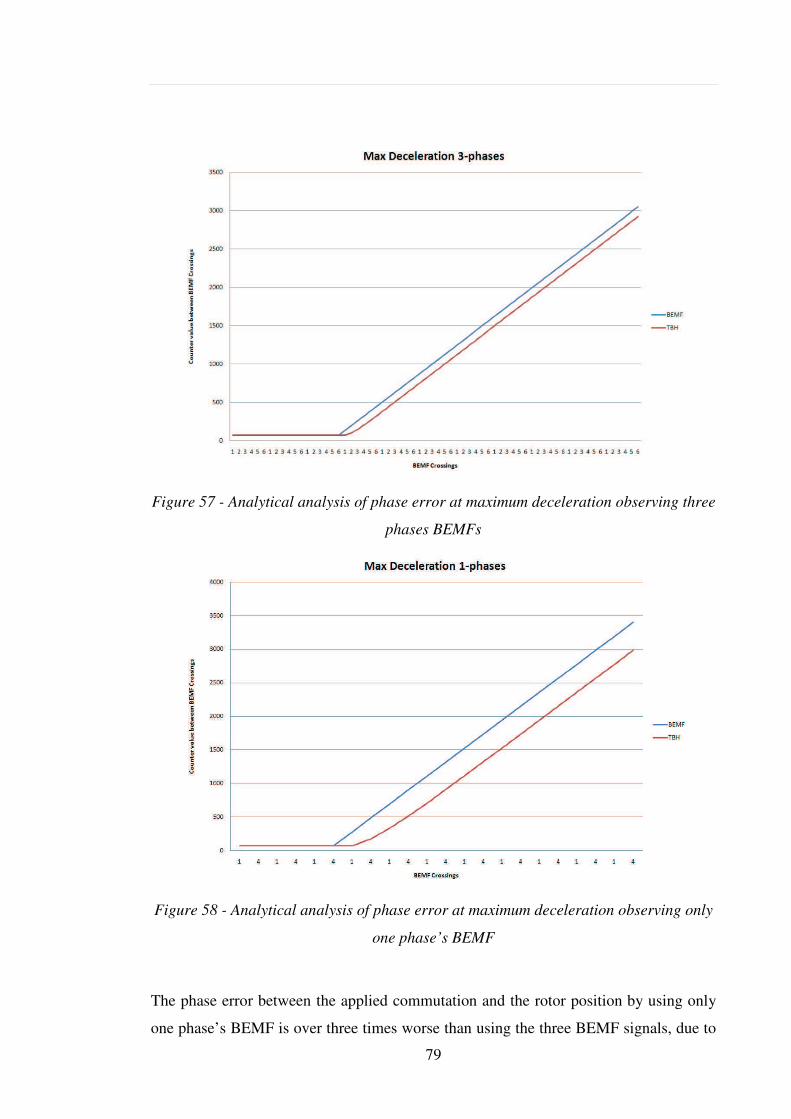
79
Figure 57 - Analytical analysis of phase error at maximum deceleration observing three
phases BEMFs
Figure 58 - Analytical analysis of phase error at maximum deceleration observing only
one phase’s BEMF
The phase error between the applied commutation and the rotor position by using only
one phase’s BEMF is over three times worse than using the three BEMF signals, due to
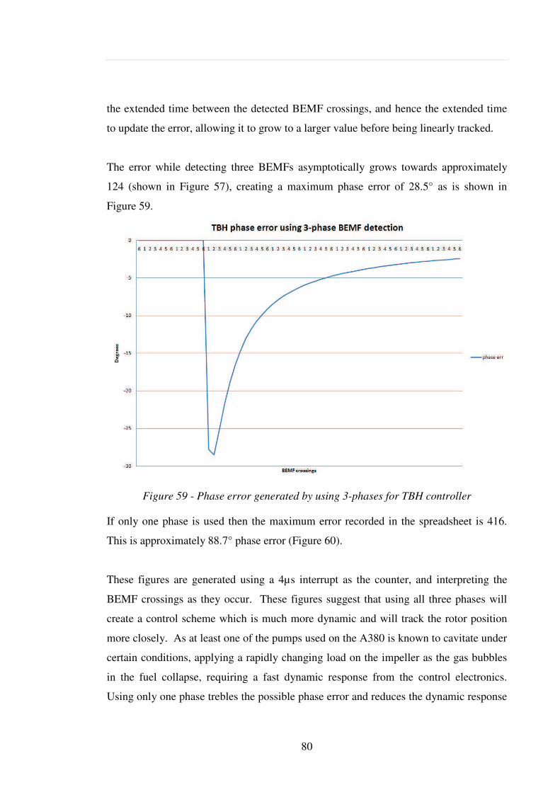
80
the extended time between the detected BEMF crossings, and hence the extended time
to update the error, allowing it to grow to a larger value before being linearly tracked.
The error while detecting three BEMFs asymptotically grows towards approximately
124 (shown in Figure 57), creating a maximum phase error of 28.5° as is shown in
Figure 59.
Figure 59 - Phase error generated by using 3-phases for TBH controller
If only one phase is used then the maximum error recorded in the spreadsheet is 416.
This is approximately 88.7° phase error (Figure 60).
These figures are generated using a 4µs interrupt as the counter, and interpreting the
BEMF crossings as they occur. These figures suggest that using all three phases will
create a control scheme which is much more dynamic and will track the rotor position
more closely. As at least one of the pumps used on the A380 is known to cavitate under
certain conditions, applying a rapidly changing load on the impeller as the gas bubbles
in the fuel collapse, requiring a fast dynamic response from the control electronics.
Using only one phase trebles the possible phase error and reduces the dynamic response
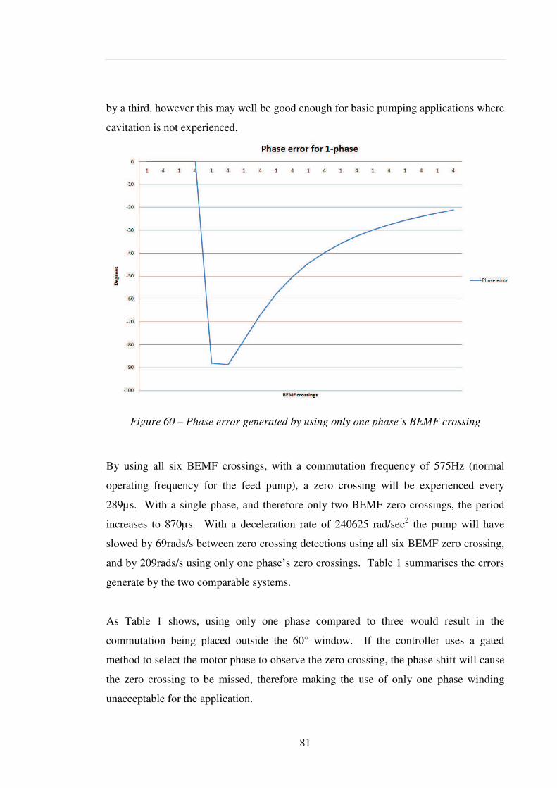
81
by a third, however this may well be good enough for basic pumping applications where
cavitation is not experienced.
Figure 60 – Phase error generated by using only one phase’s BEMF crossing
By using all six BEMF crossings, with a commutation frequency of 575Hz (normal
operating frequency for the feed pump), a zero crossing will be experienced every
289µs. With a single phase, and therefore only two BEMF zero crossings, the period
increases to 870µs. With a deceleration rate of 240625 rad/sec2 the pump will have
slowed by 69rads/s between zero crossing detections using all six BEMF zero crossing,
and by 209rads/s using only one phase’s zero crossings. Table 1 summarises the errors
generate by the two comparable systems.
As Table 1 shows, using only one phase compared to three would result in the
commutation being placed outside the 60° window. If the controller uses a gated
method to select the motor phase to observe the zero crossing, the phase shift will cause
the zero crossing to be missed, therefore making the use of only one phase winding
unacceptable for the application.
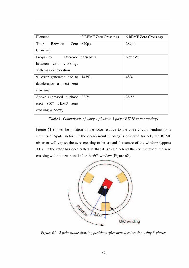
82
Element 2 BEMF Zero Crossings 6 BEMF Zero Crossings
Time Between Zero
Crossings
870µs 289µs
Frequency Decrease
between zero crossings
with max deceleration
209rads/s 69rads/s
% error generated due to
deceleration at next zero
crossing
148% 48%
Above expressed in phase
error (60° BEMF zero
crossing window)
88.7° 28.5°
Table 1- Comparison of using 1 phase to 3 phase BEMF zero crossings
Figure 61 shows the position of the rotor relative to the open circuit winding for a
simplified 2-pole motor. If the open circuit winding is observed for 60°, the BEMF
observer will expect the zero crossing to be around the centre of the window (approx
30°). If the rotor has decelerated so that it is >30° behind the commutation, the zero
crossing will not occur until after the 60° window (Figure 62).
Figure 61 - 2 pole motor showing positions after max deceleration using 3-phases
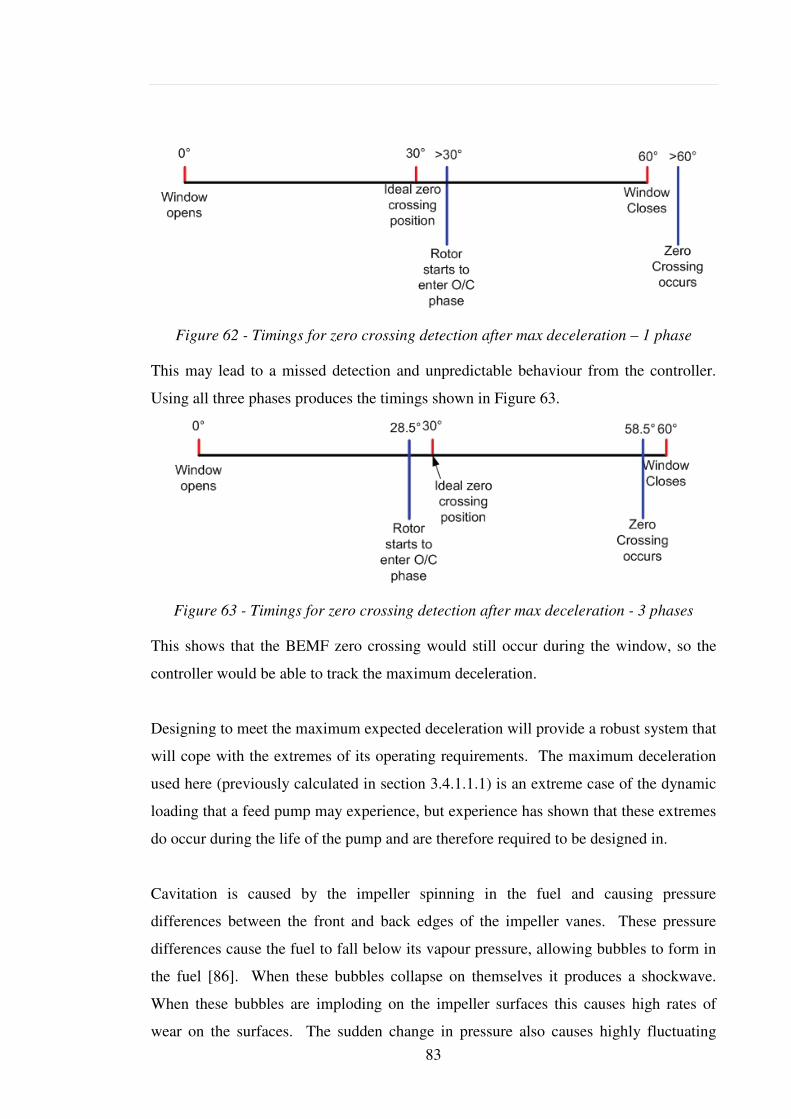
83
Figure 62 - Timings for zero crossing detection after max deceleration – 1 phase
This may lead to a missed detection and unpredictable behaviour from the controller.
Using all three phases produces the timings shown in Figure 63.
Figure 63 - Timings for zero crossing detection after max deceleration - 3 phases
This shows that the BEMF zero crossing would still occur during the window, so the
controller would be able to track the maximum deceleration.
Designing to meet the maximum expected deceleration will provide a robust system that
will cope with the extremes of its operating requirements. The maximum deceleration
used here (previously calculated in section 3.4.1.1.1) is an extreme case of the dynamic
loading that a feed pump may experience, but experience has shown that these extremes
do occur during the life of the pump and are therefore required to be designed in.
Cavitation is caused by the impeller spinning in the fuel and causing pressure
differences between the front and back edges of the impeller vanes. These pressure
differences cause the fuel to fall below its vapour pressure, allowing bubbles to form in
the fuel [86]. When these bubbles collapse on themselves it produces a shockwave.
When these bubbles are imploding on the impeller surfaces this causes high rates of
wear on the surfaces. The sudden change in pressure also causes highly fluctuating
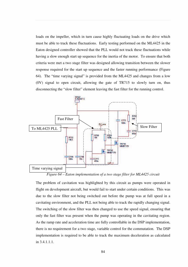
84
loads on the impeller, which in turn cause highly fluctuating loads on the drive which
must be able to track these fluctuations. Early testing performed on the ML4425 in the
Eaton designed controller showed that the PLL would not track these fluctuations while
having a slow enough start up sequence for the inertia of the motor. To ensure that both
criteria were met a two stage filter was designed allowing transition between the slower
response required for the start up sequence and the faster running performance (Figure
64). The “time varying signal” is provided from the ML4425 and changes from a low
(0V) signal to open circuit, allowing the gate of TR715 to slowly turn on, thus
disconnecting the “slow filter” element leaving the fast filter for the running control.
Figure 64 – Eaton implementation of a two stage filter for ML4425 circuit
The problem of cavitation was highlighted by this circuit as pumps were operated in
flight on development aircraft, but would fail to start under certain conditions. This was
due to the slow filter not being switched out before the pump was at full speed in a
cavitating environment, and the PLL not being able to track the rapidly changing signal.
The switching of the slow filter was then changed to use the speed signal, ensuring that
only the fast filter was present when the pump was operating in the cavitating region.
As the ramp rate and acceleration time are fully controllable in the DSP implementation,
there is no requirement for a two stage, variable control for the commutation. The DSP
implementation is required to be able to track the maximum deceleration as calculated
in 3.4.1.1.1.
To ML4425 PLL
Time varying signal
Slow Filter
Fast Filter
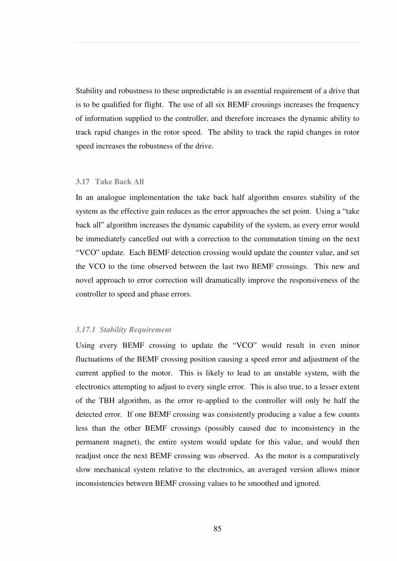
85
Stability and robustness to these unpredictable is an essential requirement of a drive that
is to be qualified for flight. The use of all six BEMF crossings increases the frequency
of information supplied to the controller, and therefore increases the dynamic ability to
track rapid changes in the rotor speed. The ability to track the rapid changes in rotor
speed increases the robustness of the drive.
3.17 Take Back All
In an analogue implementation the take back half algorithm ensures stability of the
system as the effective gain reduces as the error approaches the set point. Using a “take
back all” algorithm increases the dynamic capability of the system, as every error would
be immediately cancelled out with a correction to the commutation timing on the next
“VCO” update. Each BEMF detection crossing would update the counter value, and set
the VCO to the time observed between the last two BEMF crossings. This new and
novel approach to error correction will dramatically improve the responsiveness of the
controller to speed and phase errors.
3.17.1 Stability Requirement
Using every BEMF crossing to update the “VCO” would result in even minor
fluctuations of the BEMF crossing position causing a speed error and adjustment of the
current applied to the motor. This is likely to lead to an unstable system, with the
electronics attempting to adjust to every single error. This is also true, to a lesser extent
of the TBH algorithm, as the error re-applied to the controller will only be half the
detected error. If one BEMF crossing was consistently producing a value a few counts
less than the other BEMF crossings (possibly caused due to inconsistency in the
permanent magnet), the entire system would update for this value, and would then
readjust once the next BEMF crossing was observed. As the motor is a comparatively
slow mechanical system relative to the electronics, an averaged version allows minor
inconsistencies between BEMF crossing values to be smoothed and ignored.
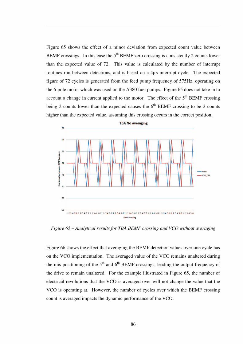
86
Figure 65 shows the effect of a minor deviation from expected count value between
BEMF crossings. In this case the 5th BEMF zero crossing is consistently 2 counts lower
than the expected value of 72. This value is calculated by the number of interrupt
routines run between detections, and is based on a 4µs interrupt cycle. The expected
figure of 72 cycles is generated from the feed pump frequency of 575Hz, operating on
the 6-pole motor which was used on the A380 fuel pumps. Figure 65 does not take in to
account a change in current applied to the motor. The effect of the 5th BEMF crossing
being 2 counts lower than the expected causes the 6th BEMF crossing to be 2 counts
higher than the expected value, assuming this crossing occurs in the correct position.
Figure 65 – Analytical results for TBA BEMF crossing and VCO without averaging
Figure 66 shows the effect that averaging the BEMF detection values over one cycle has
on the VCO implementation. The averaged value of the VCO remains unaltered during
the mis-positioning of the 5th and 6th BEMF crossings, leading the output frequency of
the drive to remain unaltered. For the example illustrated in Figure 65, the number of
electrical revolutions that the VCO is averaged over will not change the value that the
VCO is operating at. However, the number of cycles over which the BEMF crossing
count is averaged impacts the dynamic performance of the VCO.
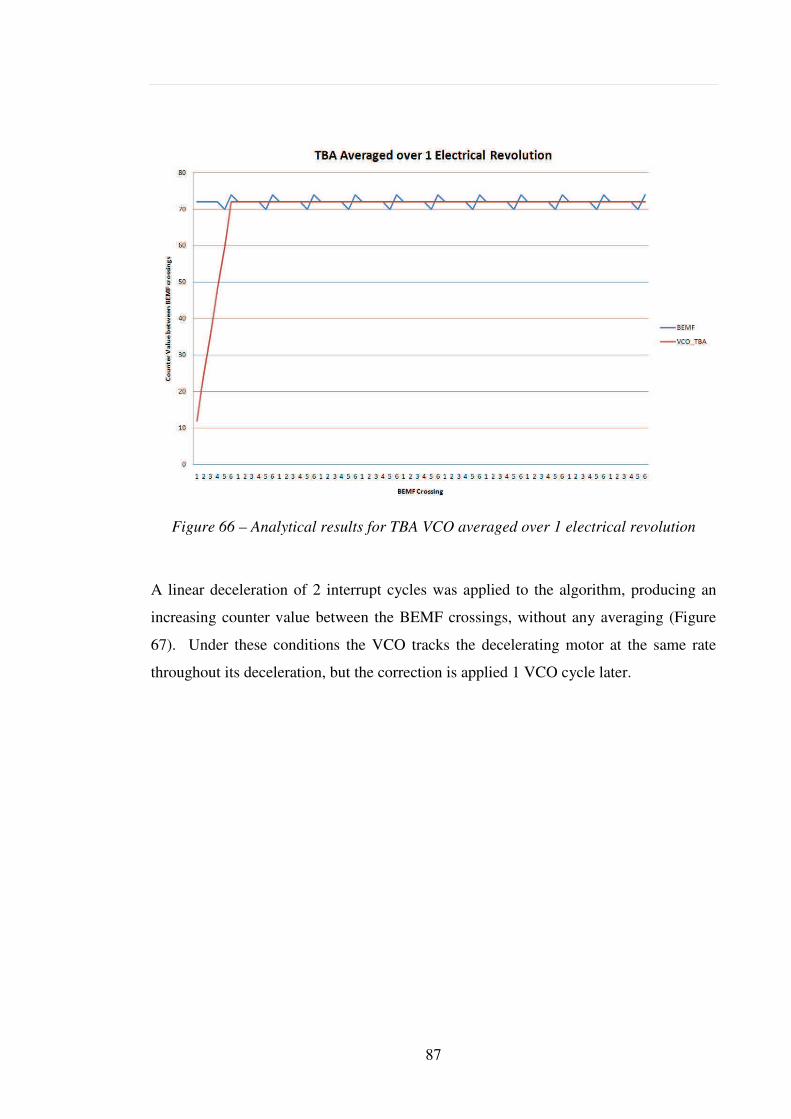
87
Figure 66 – Analytical results for TBA VCO averaged over 1 electrical revolution
A linear deceleration of 2 interrupt cycles was applied to the algorithm, producing an
increasing counter value between the BEMF crossings, without any averaging (Figure
67). Under these conditions the VCO tracks the decelerating motor at the same rate
throughout its deceleration, but the correction is applied 1 VCO cycle later.
88
Figure 67 – Analytical results for TBA without averaging under deceleration
Averaging the signal over 1 electrical cycle increases the error between the BEMF
count and the VCO count, as can been seen between Figure 67 and Figure 68. The first
electrical revolution under deceleration determines the error that will be generated
throughout the linear deceleration, as the signal is averaged over only 1 electrical
revolution.
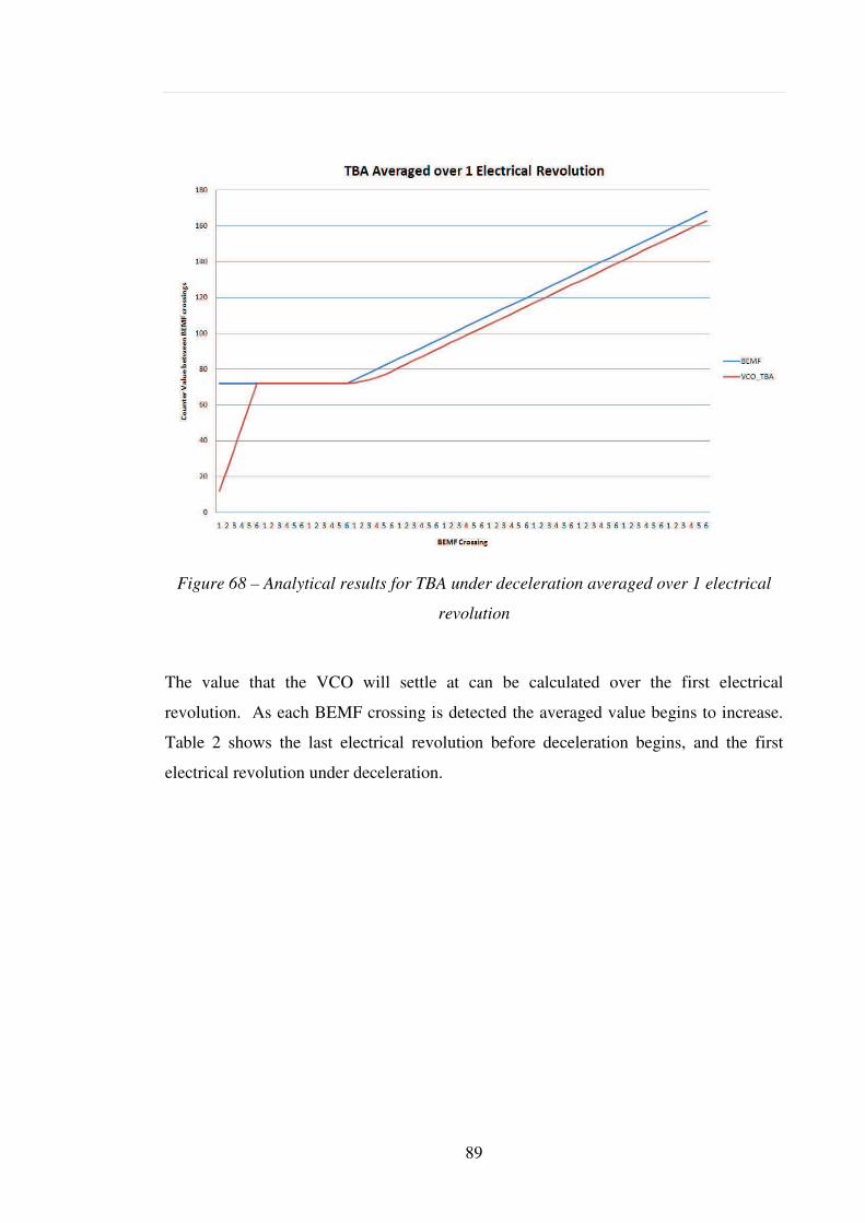
89
Figure 68 – Analytical results for TBA under deceleration averaged over 1 electrical
revolution
The value that the VCO will settle at can be calculated over the first electrical
revolution. As each BEMF crossing is detected the averaged value begins to increase.
Table 2 shows the last electrical revolution before deceleration begins, and the first
electrical revolution under deceleration.
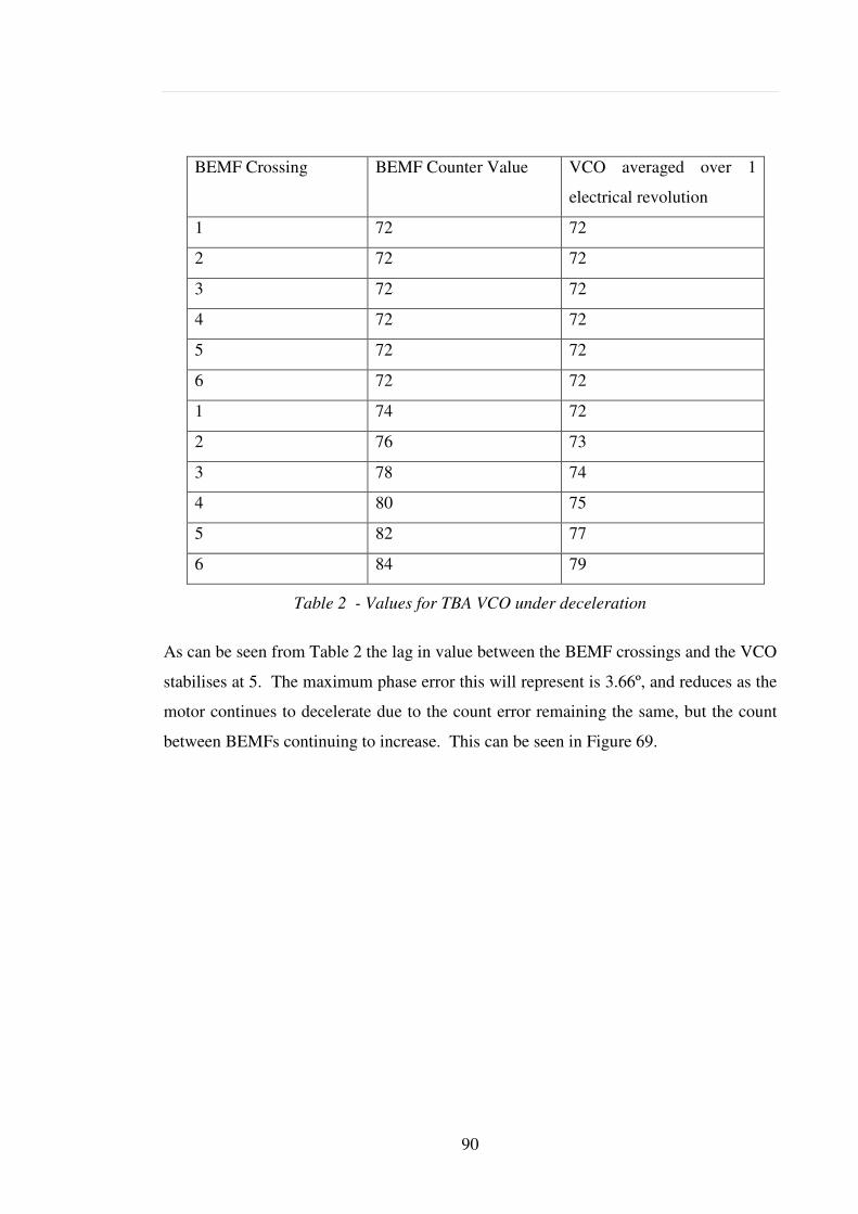
90
BEMF Crossing BEMF Counter Value VCO averaged over 1
electrical revolution
1 72 72
2 72 72
3 72 72
4 72 72
5 72 72
6 72 72
1 74 72
2 76 73
3 78 74
4 80 75
5 82 77
6 84 79
Table 2 - Values for TBA VCO under deceleration
As can be seen from Table 2 the lag in value between the BEMF crossings and the VCO
stabilises at 5. The maximum phase error this will represent is 3.66º, and reduces as the
motor continues to decelerate due to the count error remaining the same, but the count
between BEMFs continuing to increase. This can be seen in Figure 69.
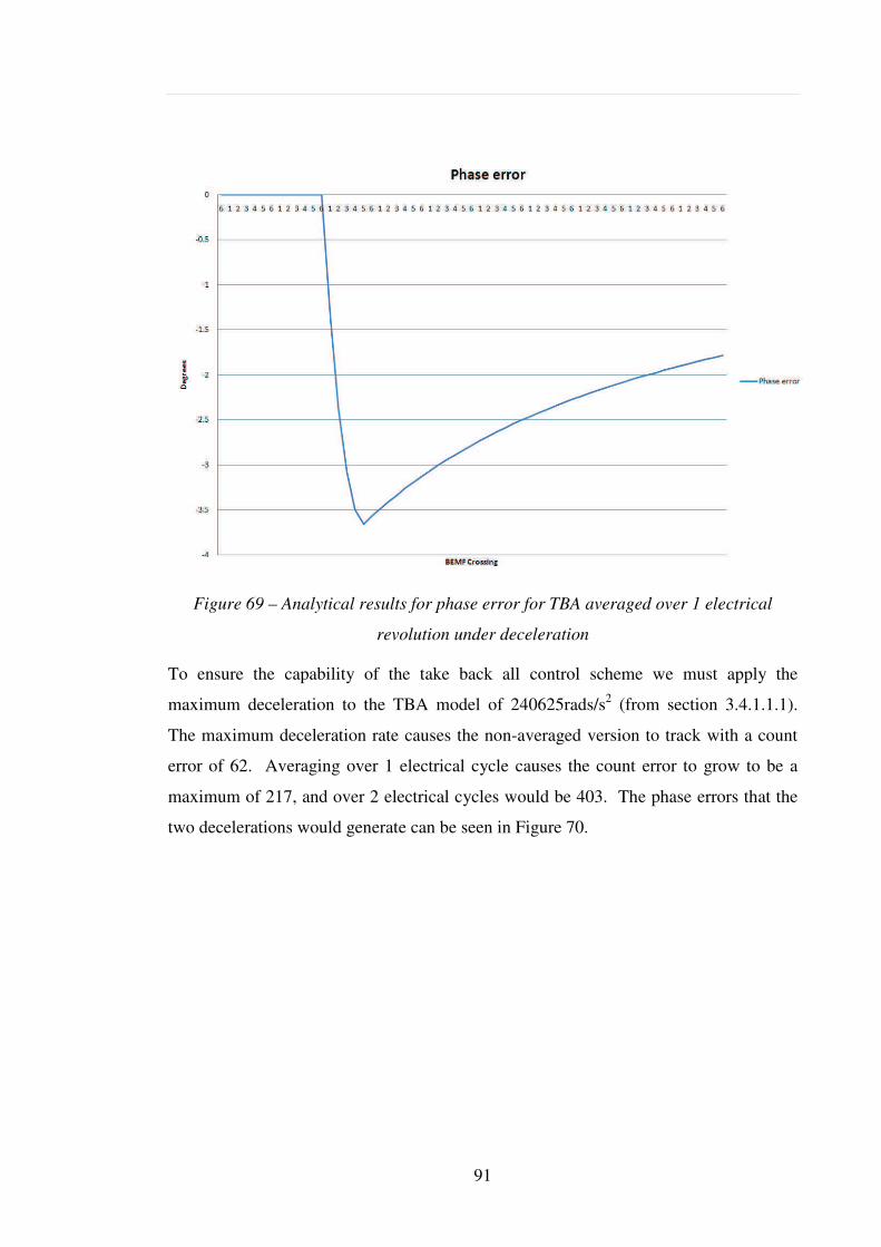
91
Figure 69 – Analytical results for phase error for TBA averaged over 1 electrical
revolution under deceleration
To ensure the capability of the take back all control scheme we must apply the
maximum deceleration to the TBA model of 240625rads/s2 (from section 3.4.1.1.1).
The maximum deceleration rate causes the non-averaged version to track with a count
error of 62. Averaging over 1 electrical cycle causes the count error to grow to be a
maximum of 217, and over 2 electrical cycles would be 403. The phase errors that the
two decelerations would generate can be seen in Figure 70.
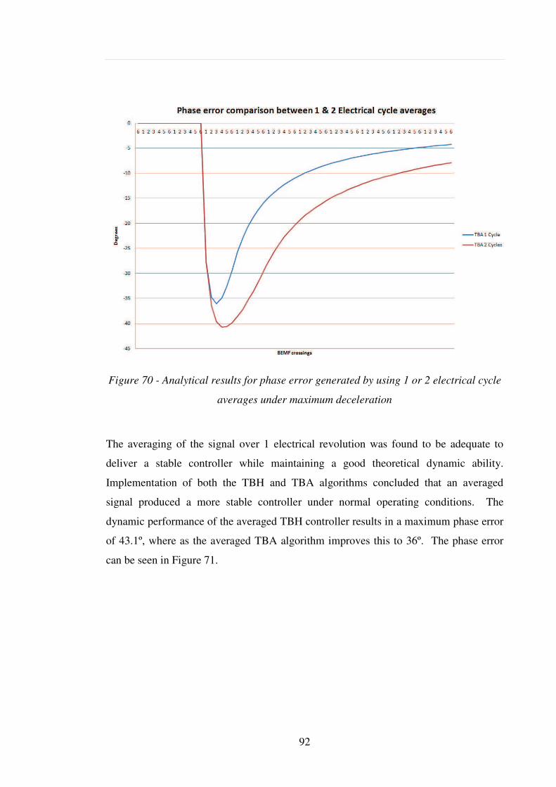
92
Figure 70 - Analytical results for phase error generated by using 1 or 2 electrical cycle
averages under maximum deceleration
The averaging of the signal over 1 electrical revolution was found to be adequate to
deliver a stable controller while maintaining a good theoretical dynamic ability.
Implementation of both the TBH and TBA algorithms concluded that an averaged
signal produced a more stable controller under normal operating conditions. The
dynamic performance of the averaged TBH controller results in a maximum phase error
of 43.1º, where as the averaged TBA algorithm improves this to 36º. The phase error
can be seen in Figure 71.
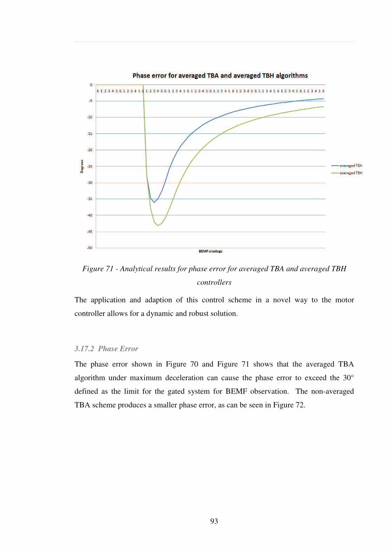
93
Figure 71 - Analytical results for phase error for averaged TBA and averaged TBH
controllers
The application and adaption of this control scheme in a novel way to the motor
controller allows for a dynamic and robust solution.
3.17.2 Phase Error
The phase error shown in Figure 70 and Figure 71 shows that the averaged TBA
algorithm under maximum deceleration can cause the phase error to exceed the 30°
defined as the limit for the gated system for BEMF observation. The non-averaged
TBA scheme produces a smaller phase error, as can be seen in Figure 72.
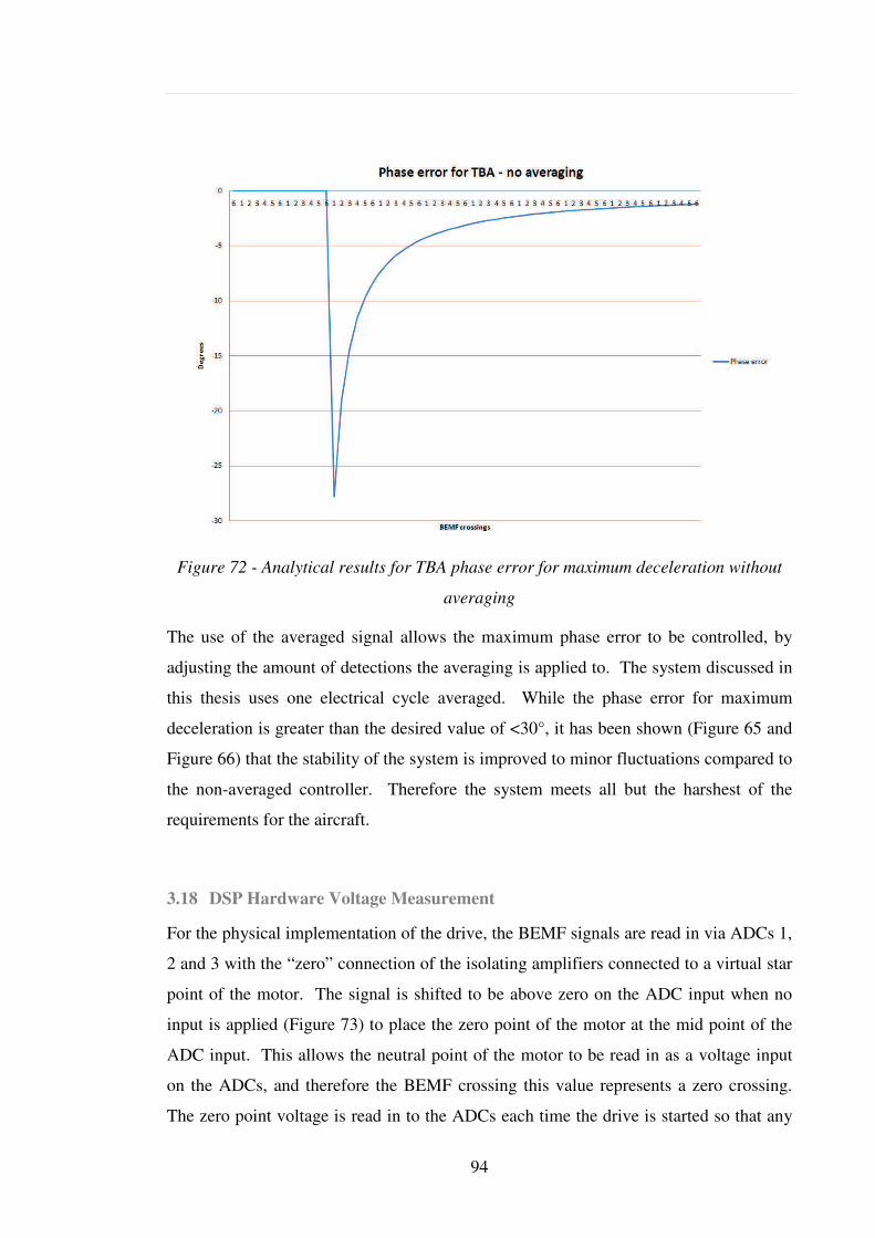
94
Figure 72 - Analytical results for TBA phase error for maximum deceleration without
averaging
The use of the averaged signal allows the maximum phase error to be controlled, by
adjusting the amount of detections the averaging is applied to. The system discussed in
this thesis uses one electrical cycle averaged. While the phase error for maximum
deceleration is greater than the desired value of <30°, it has been shown (Figure 65 and
Figure 66) that the stability of the system is improved to minor fluctuations compared to
the non-averaged controller. Therefore the system meets all but the harshest of the
requirements for the aircraft.
3.18 DSP Hardware Voltage Measurement
For the physical implementation of the drive, the BEMF signals are read in via ADCs 1,
2 and 3 with the “zero” connection of the isolating amplifiers connected to a virtual star
point of the motor. The signal is shifted to be above zero on the ADC input when no
input is applied (Figure 73) to place the zero point of the motor at the mid point of the
ADC input. This allows the neutral point of the motor to be read in as a voltage input
on the ADCs, and therefore the BEMF crossing this value represents a zero crossing.
The zero point voltage is read in to the ADCs each time the drive is started so that any
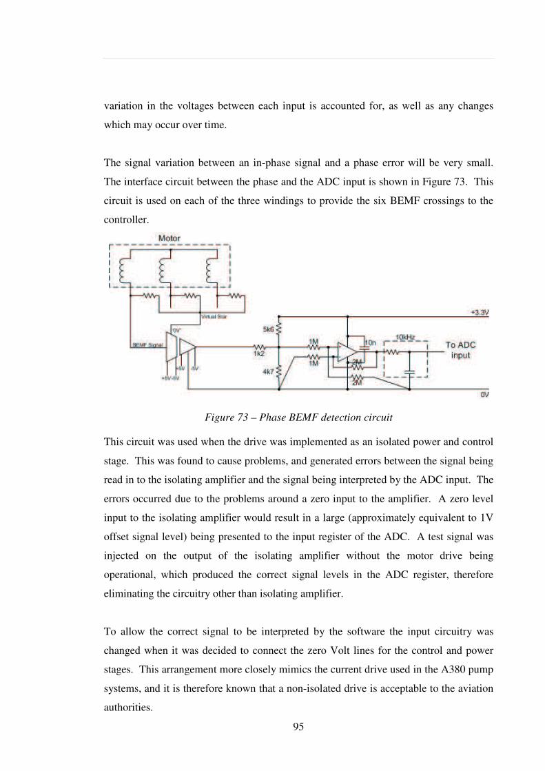
95
variation in the voltages between each input is accounted for, as well as any changes
which may occur over time.
The signal variation between an in-phase signal and a phase error will be very small.
The interface circuit between the phase and the ADC input is shown in Figure 73. This
circuit is used on each of the three windings to provide the six BEMF crossings to the
controller.
Figure 73 – Phase BEMF detection circuit
This circuit was used when the drive was implemented as an isolated power and control
stage. This was found to cause problems, and generated errors between the signal being
read in to the isolating amplifier and the signal being interpreted by the ADC input. The
errors occurred due to the problems around a zero input to the amplifier. A zero level
input to the isolating amplifier would result in a large (approximately equivalent to 1V
offset signal level) being presented to the input register of the ADC. A test signal was
injected on the output of the isolating amplifier without the motor drive being
operational, which produced the correct signal levels in the ADC register, therefore
eliminating the circuitry other than isolating amplifier.
To allow the correct signal to be interpreted by the software the input circuitry was
changed when it was decided to connect the zero Volt lines for the control and power
stages. This arrangement more closely mimics the current drive used in the A380 pump
systems, and it is therefore known that a non-isolated drive is acceptable to the aviation
authorities.
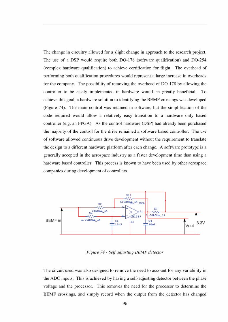
96
The change in circuitry allowed for a slight change in approach to the research project.
The use of a DSP would require both DO-178 (software qualification) and DO-254
(complex hardware qualification) to achieve certification for flight. The overhead of
performing both qualification procedures would represent a large increase in overheads
for the company. The possibility of removing the overhead of DO-178 by allowing the
controller to be easily implemented in hardware would be greatly beneficial. To
achieve this goal, a hardware solution to identifying the BEMF crossings was developed
(Figure 74). The main control was retained in software, but the simplification of the
code required would allow a relatively easy transition to a hardware only based
controller (e.g. an FPGA). As the control hardware (DSP) had already been purchased
the majority of the control for the drive remained a software based controller. The use
of software allowed continuous drive development without the requirement to translate
the design to a different hardware platform after each change. A software prototype is a
generally accepted in the aerospace industry as a faster development time than using a
hardware based controller. This process is known to have been used by other aerospace
companies during development of controllers.
Figure 74 - Self adjusting BEMF detector
The circuit used was also designed to remove the need to account for any variability in
the ADC inputs. This is achieved by having a self-adjusting detector between the phase
voltage and the processor. This removes the need for the processor to determine the
BEMF crossings, and simply record when the output from the detector has changed
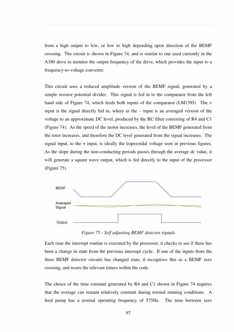
97
from a high output to low, or low to high depending upon direction of the BEMF
crossing. The circuit is shown in Figure 74, and is similar to one used currently in the
A380 drive to monitor the output frequency of the drive, which provides the input to a
frequency-to-voltage converter.
This circuit uses a reduced amplitude version of the BEMF signal, generated by a
simple resistor potential divider. This signal is fed in to the comparator from the left
hand side of Figure 74, which feeds both inputs of the comparator (LM139J). The +
input is the signal directly fed in, where as the – input is an averaged version of the
voltage to an approximate DC level, produced by the RC filter consisting of R4 and C1
(Figure 74). As the speed of the motor increases, the level of the BEMF generated from
the rotor increases, and therefore the DC level generated from the signal increases. The
signal input, to the + input, is ideally the trapezoidal voltage seen in previous figures.
As the slope during the non-conducting periods passes through the average dc value, it
will generate a square wave output, which is fed directly to the input of the processor
(Figure 75).
Figure 75 - Self adjusting BEMF detector signals
Each time the interrupt routine is executed by the processor, it checks to see if there has
been a change in state from the previous interrupt cycle. If one of the inputs from the
three BEMF detector circuits has changed state, it recognises this as a BEMF zero
crossing, and resets the relevant timers within the code.
The choice of the time constant generated by R4 and C1 shown in Figure 74 requires
that the average can remain relatively constant during normal running conditions. A
feed pump has a normal operating frequency of 575Hz. The time between zero

98
crossings on each phase is therefore 870S. The time constant for the RC filter R4 and
C1 uses 1M and 15nF, which provides a 15mS time constant. As the average value of
the signal is required to remain relatively constant, but be able to adjust if the signal
fluctuates greatly. The 20x time constant that was chosen is a compromise between
responsiveness to speed changes, and maintaining a relatively constant voltage during
normal operation. If the drive were to be implemented on a motor running at a much
higher or much lower speed the values for the time constant may require adjustment to
maintain an acceptable level or ripple/responsiveness to changing speed on the averaged
input to the op-amp.
3.19 Current measurement
The current is measured using a DC link current shunt resistor in the negative rail. This
signal is amplified on the power side and then fed through an isolating amplifier to the
control side.
The gain of the circuit (Figure 76) is 10 (1 + 9k/1k). A 30 amp DC current passing
through Rsense (0.005 ) will produce a voltage of 0.15V across it. This will produce a
voltage of 1.5V on the output of the op-amp. The output of the circuit is fed through an
isolating amplifier to a non-inverting amplifier with a gain of two. This second
amplification stage serves two purposes:
1. To amplify the signal to the maximum range of the ADC input (0 – 3V).
2. To limit the voltage applied to the ADC input to below 3.3V and above -0.4V,
the maximum input limits for the processor.
Figure 76 – Current measurement circuit
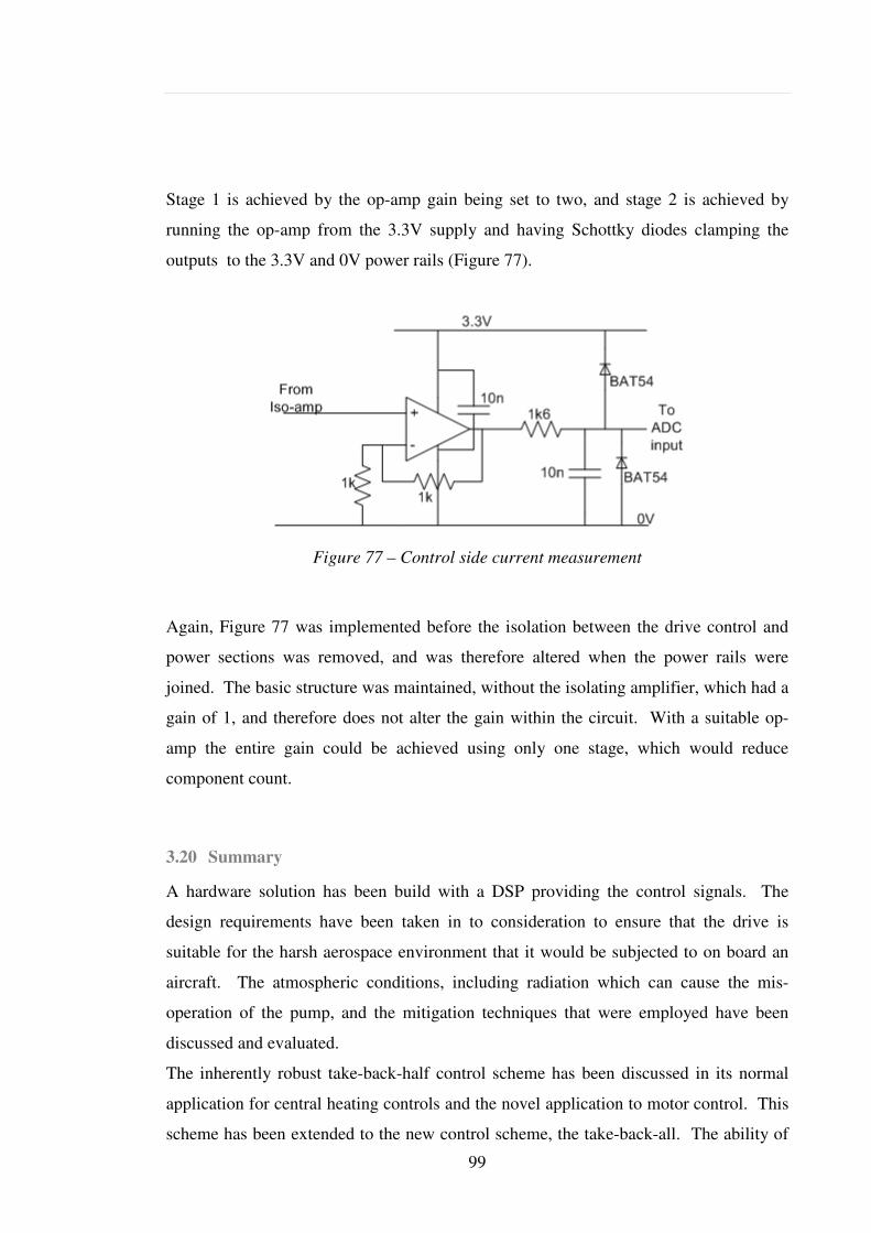
99
Stage 1 is achieved by the op-amp gain being set to two, and stage 2 is achieved by
running the op-amp from the 3.3V supply and having Schottky diodes clamping the
outputs to the 3.3V and 0V power rails (Figure 77).
Figure 77 – Control side current measurement
Again, Figure 77 was implemented before the isolation between the drive control and
power sections was removed, and was therefore altered when the power rails were
joined. The basic structure was maintained, without the isolating amplifier, which had a
gain of 1, and therefore does not alter the gain within the circuit. With a suitable op-
amp the entire gain could be achieved using only one stage, which would reduce
component count.
3.20 Summary
A hardware solution has been build with a DSP providing the control signals. The
design requirements have been taken in to consideration to ensure that the drive is
suitable for the harsh aerospace environment that it would be subjected to on board an
aircraft. The atmospheric conditions, including radiation which can cause the mis-
operation of the pump, and the mitigation techniques that were employed have been
discussed and evaluated.
The inherently robust take-back-half control scheme has been discussed in its normal
application for central heating controls and the novel application to motor control. This
scheme has been extended to the new control scheme, the take-back-all. The ability of

100
the system to almost immediately correct errors improves the dynamic response to
changes in load, and allows the controller to more closely meet the maximum
deceleration rates that it may encounter. The combination of this new control scheme,
with the novel PWM application (as described in 3.14 ) has been produced using
minimal hardware, in a manner that would allow simple transition to a hardware only
controller.
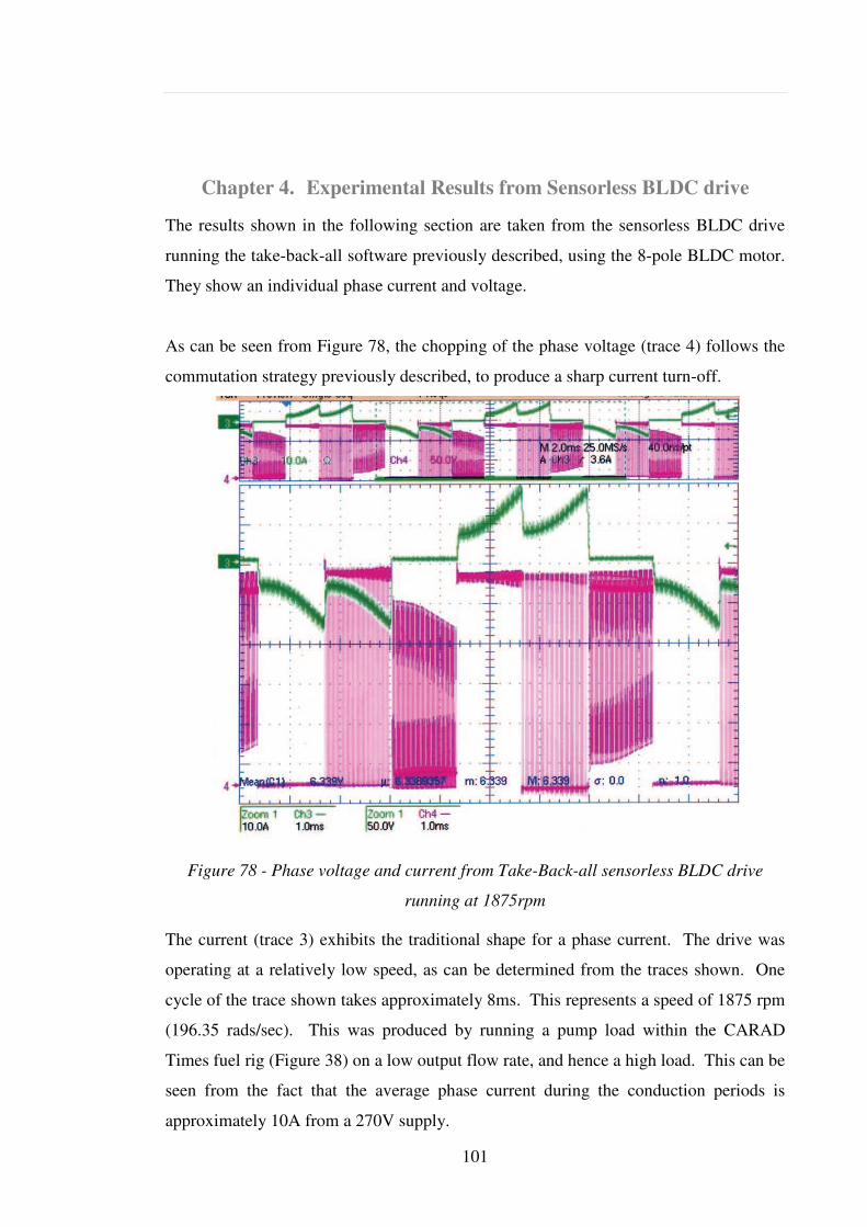
101
Chapter 4. Experimental Results from Sensorless BLDC drive
The results shown in the following section are taken from the sensorless BLDC drive
running the take-back-all software previously described, using the 8-pole BLDC motor.
They show an individual phase current and voltage.
As can be seen from Figure 78, the chopping of the phase voltage (trace 4) follows the
commutation strategy previously described, to produce a sharp current turn-off.
Figure 78 - Phase voltage and current from Take-Back-all sensorless BLDC drive
running at 1875rpm
The current (trace 3) exhibits the traditional shape for a phase current. The drive was
operating at a relatively low speed, as can be determined from the traces shown. One
cycle of the trace shown takes approximately 8ms. This represents a speed of 1875 rpm
(196.35 rads/sec). This was produced by running a pump load within the CARAD
Times fuel rig (Figure 38) on a low output flow rate, and hence a high load. This can be
seen from the fact that the average phase current during the conduction periods is
approximately 10A from a 270V supply.

102
The same speed run can be seen in Figure 79 driving a dry running motor (not pumping
fuel, therefore on effectively no-load).
In Figure 79 the Voltage (trace 4) is still set at 270Vdc, but the average phase current
(trace 3) is approximately 1A to control the speed to be the same as in Figure 78.
Figure 79 - No-load pump running at 1875rpm (Trace 3 = phase current, Trace 4=
phase voltage)
The current is controlled to reduce the applied torque to match the load torque. This is
evident when the pump has changed from running in fuel in Figure 78 (applies load the
impeller of the pump) to the no load situation in Figure 79 of a pump running unloaded
in free air. As described previously, the level of current applied alters the speed of the
motor, thus ensuring that this is controlled properly ensures that the pump runs at the
desired speed. The evidence from Figure 78 and Figure 79 shows that the pump
2ms/div
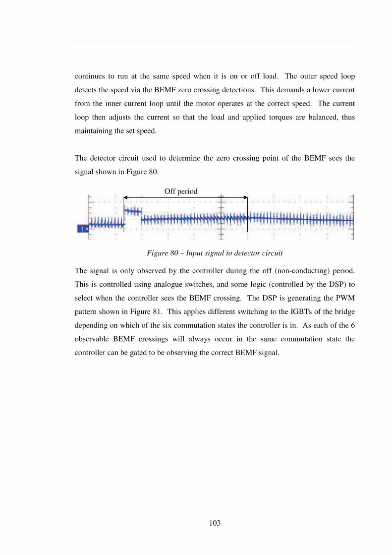
103
continues to run at the same speed when it is on or off load. The outer speed loop
detects the speed via the BEMF zero crossing detections. This demands a lower current
from the inner current loop until the motor operates at the correct speed. The current
loop then adjusts the current so that the load and applied torques are balanced, thus
maintaining the set speed.
The detector circuit used to determine the zero crossing point of the BEMF sees the
signal shown in Figure 80.
Figure 80 – Input signal to detector circuit
The signal is only observed by the controller during the off (non-conducting) period.
This is controlled using analogue switches, and some logic (controlled by the DSP) to
select when the controller sees the BEMF crossing. The DSP is generating the PWM
pattern shown in Figure 81. This applies different switching to the IGBTs of the bridge
depending on which of the six commutation states the controller is in. As each of the 6
observable BEMF crossings will always occur in the same commutation state the
controller can be gated to be observing the correct BEMF signal.
Off period
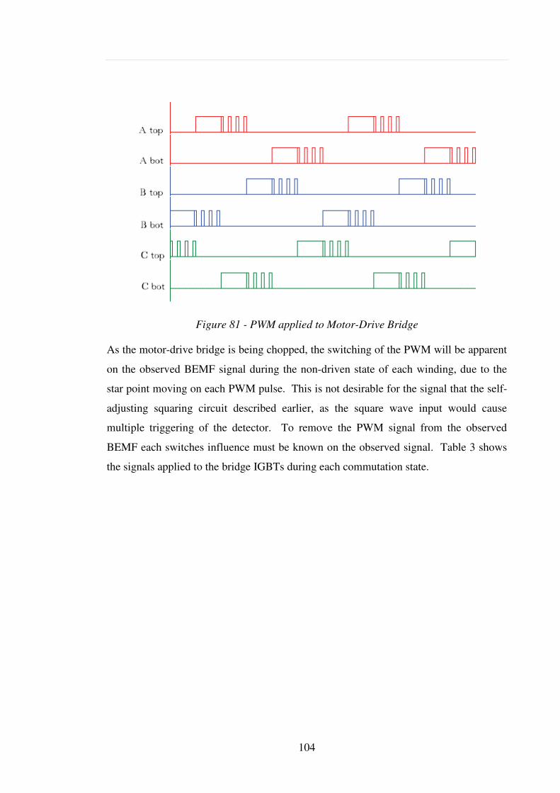
104
Figure 81 - PWM applied to Motor-Drive Bridge
As the motor-drive bridge is being chopped, the switching of the PWM will be apparent
on the observed BEMF signal during the non-driven state of each winding, due to the
star point moving on each PWM pulse. This is not desirable for the signal that the self-
adjusting squaring circuit described earlier, as the square wave input would cause
multiple triggering of the detector. To remove the PWM signal from the observed
BEMF each switches influence must be known on the observed signal. Table 3 shows
the signals applied to the bridge IGBTs during each commutation state.
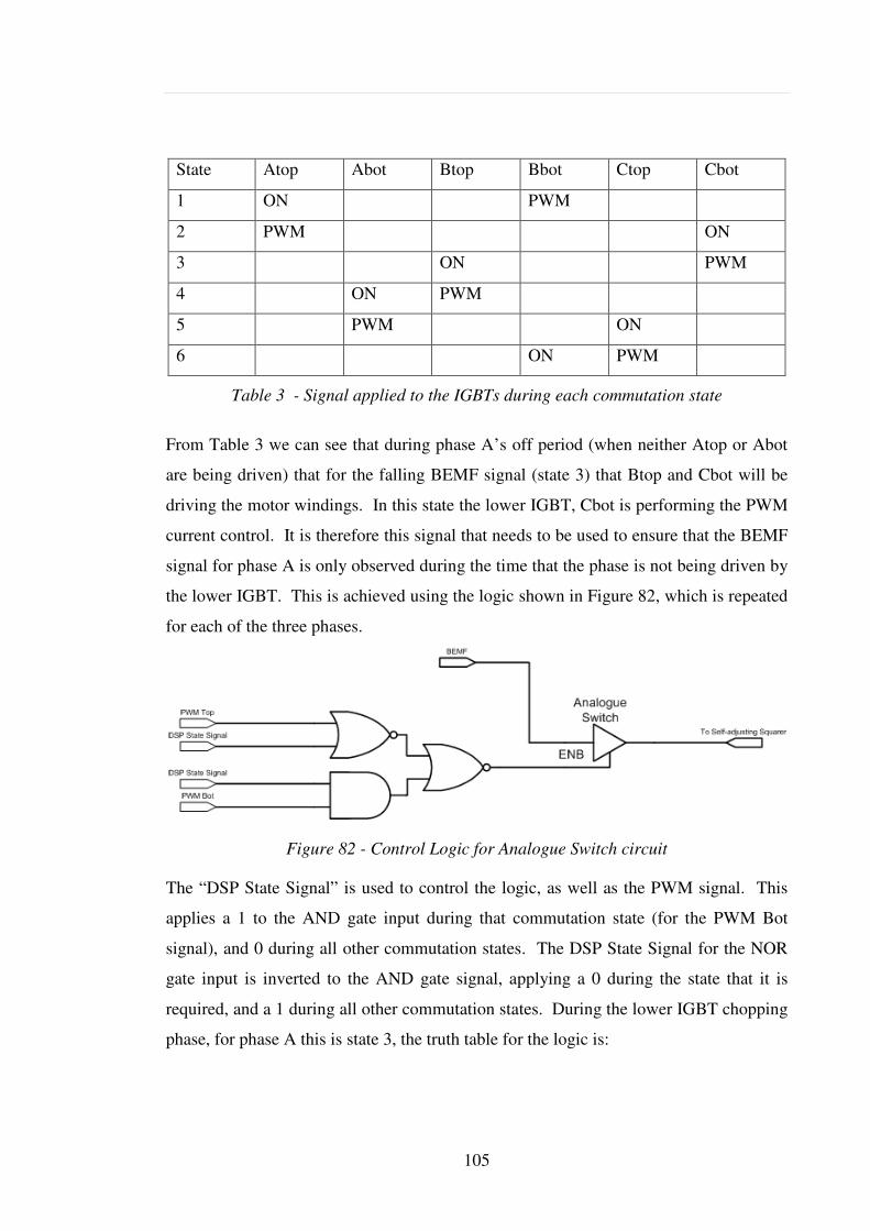
105
State Atop Abot Btop Bbot Ctop Cbot
1 ON PWM
2 PWM ON
3 ON PWM
4 ON PWM
5 PWM ON
6 ON PWM
Table 3 - Signal applied to the IGBTs during each commutation state
From Table 3 we can see that during phase A’s off period (when neither Atop or Abot
are being driven) that for the falling BEMF signal (state 3) that Btop and Cbot will be
driving the motor windings. In this state the lower IGBT, Cbot is performing the PWM
current control. It is therefore this signal that needs to be used to ensure that the BEMF
signal for phase A is only observed during the time that the phase is not being driven by
the lower IGBT. This is achieved using the logic shown in Figure 82, which is repeated
for each of the three phases.
Figure 82 - Control Logic for Analogue Switch circuit
The “DSP State Signal” is used to control the logic, as well as the PWM signal. This
applies a 1 to the AND gate input during that commutation state (for the PWM Bot
signal), and 0 during all other commutation states. The DSP State Signal for the NOR
gate input is inverted to the AND gate signal, applying a 0 during the state that it is
required, and a 1 during all other commutation states. During the lower IGBT chopping
phase, for phase A this is state 3, the truth table for the logic is:
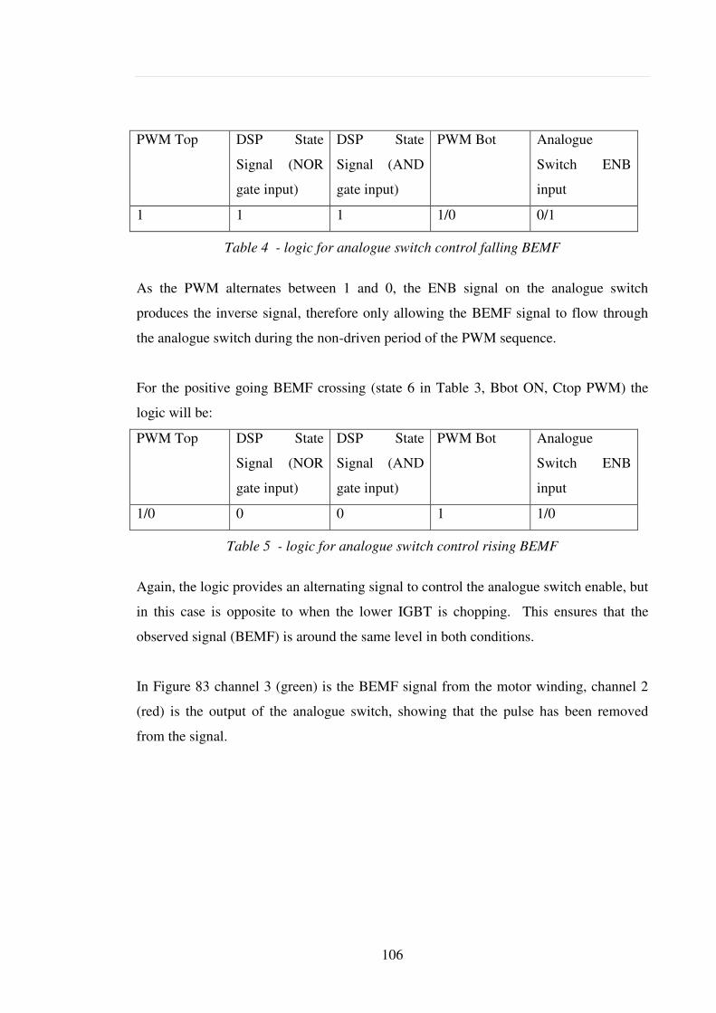
106
PWM Top DSP State
Signal (NOR
gate input)
DSP State
Signal (AND
gate input)
PWM Bot Analogue
Switch ENB
input
1 1 1 1/0 0/1
Table 4 - logic for analogue switch control falling BEMF
As the PWM alternates between 1 and 0, the ENB signal on the analogue switch
produces the inverse signal, therefore only allowing the BEMF signal to flow through
the analogue switch during the non-driven period of the PWM sequence.
For the positive going BEMF crossing (state 6 in Table 3, Bbot ON, Ctop PWM) the
logic will be:
PWM Top DSP State
Signal (NOR
gate input)
DSP State
Signal (AND
gate input)
PWM Bot Analogue
Switch ENB
input
1/0 0 0 1 1/0
Table 5 - logic for analogue switch control rising BEMF
Again, the logic provides an alternating signal to control the analogue switch enable, but
in this case is opposite to when the lower IGBT is chopping. This ensures that the
observed signal (BEMF) is around the same level in both conditions.
In Figure 83 channel 3 (green) is the BEMF signal from the motor winding, channel 2
(red) is the output of the analogue switch, showing that the pulse has been removed
from the signal.
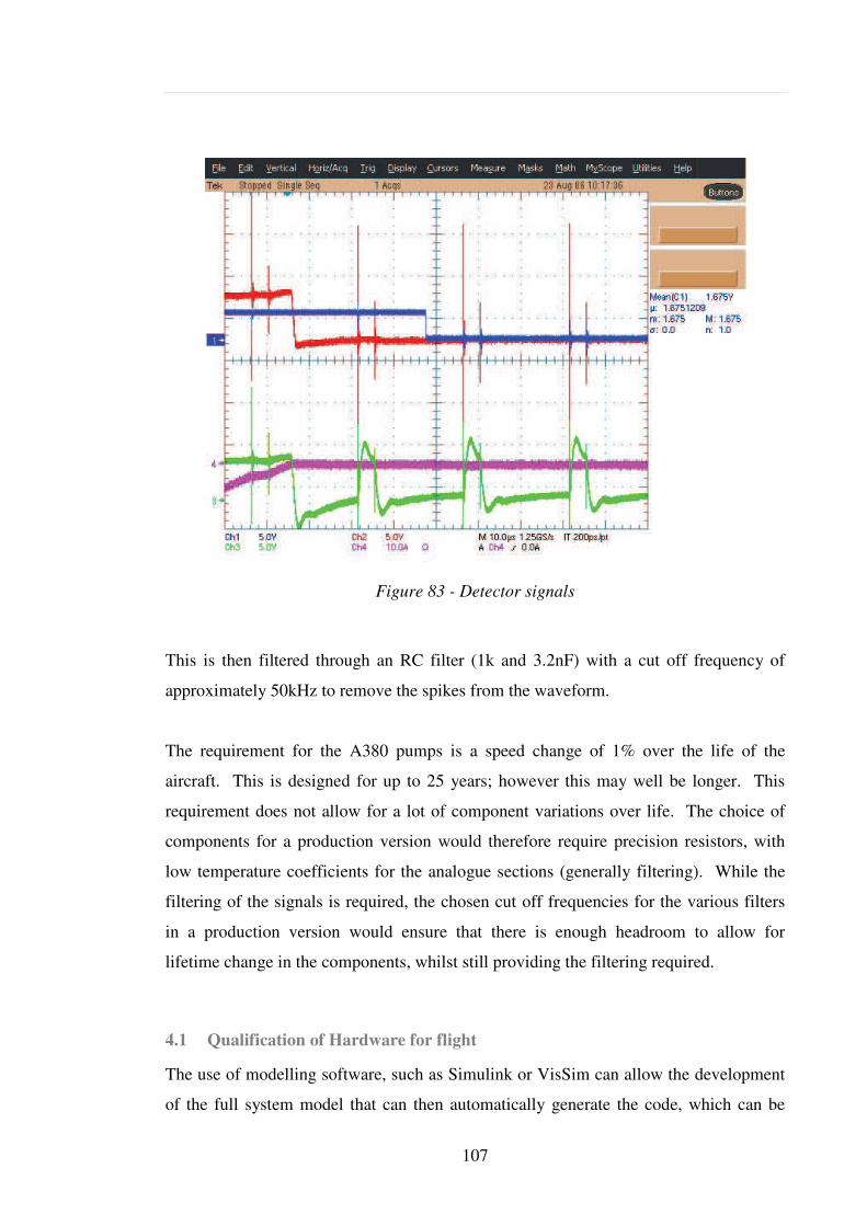
107
Figure 83 - Detector signals
This is then filtered through an RC filter (1k and 3.2nF) with a cut off frequency of
approximately 50kHz to remove the spikes from the waveform.
The requirement for the A380 pumps is a speed change of 1% over the life of the
aircraft. This is designed for up to 25 years; however this may well be longer. This
requirement does not allow for a lot of component variations over life. The choice of
components for a production version would therefore require precision resistors, with
low temperature coefficients for the analogue sections (generally filtering). While the
filtering of the signals is required, the chosen cut off frequencies for the various filters
in a production version would ensure that there is enough headroom to allow for
lifetime change in the components, whilst still providing the filtering required.
4.1 Qualification of Hardware for flight
The use of modelling software, such as Simulink or VisSim can allow the development
of the full system model that can then automatically generate the code, which can be

108
downloaded to the processor. The use of Simulink, which has a specific block set for
the TI processors, allows the standard functions of the processor to be combined with
the system model. The code generated from this model is then downloadable to the
processor directly. This code can also be used in conjunction with a SABER model,
which is required by both Airbus and Boeing for the fuel system model. Having the
ability to incorporate all of this in to one system allows full testing and alteration of the
software including testing for any cavitating effects that may be experienced on the high
speed pumps.
To qualify a software based drive for an aircraft requires a large amount of
documentation generation, analysing the software to ensure the reliability and validity
of the code. Using Simulink to generate the code for the controller allows the automatic
generation of up to 74% of the documentation required to qualify the code to DO-178
(Software) or DO-254 (Complex Hardware). This can greatly reduce the time to both
develop the code (using model based generation) and to qualify the unit. This rapid
development process, and the ability to develop a standard controller, which can be used
for multiple drives by connecting different bridge modules, increases the overall number
of controllers which in turn reduces the cost of the overall drive.
The approach taken with the drive detailed in this thesis was to allow an easy transition
to an FPGA based drive, which would remove the need for DO-178 qualification, but
would still require DO-254 qualification. The use of model based design simplifies the
ability to make rapid development changes, without the need for costly prototyping.
The ability to test with “hardware in the loop” allows minimal prototyping, simply
using the processor/FPGA attached to the model, so that the model is run at a reduced
speed to ensure that there are not problems in transition from model to hardware.
The use of a model based (Simulink / ModelSim) allows traceability of requirements
from a requirements document (DOORS database, Microsoft Word file, Microsoft
Excel file) through to the model with each section of model being linked back to a
specific requirement. While this project has been hand coded throughout, the use of
such tools would be a helpful addition to a production version of the solution. The use
of the automatic code / VHDL allows the continued traceability from the requirements
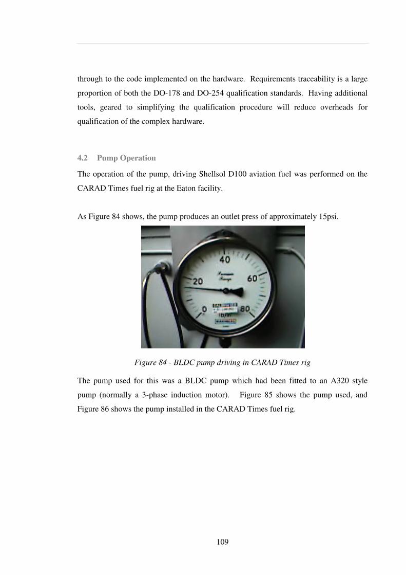
109
through to the code implemented on the hardware. Requirements traceability is a large
proportion of both the DO-178 and DO-254 qualification standards. Having additional
tools, geared to simplifying the qualification procedure will reduce overheads for
qualification of the complex hardware.
4.2 Pump Operation
The operation of the pump, driving Shellsol D100 aviation fuel was performed on the
CARAD Times fuel rig at the Eaton facility.
As Figure 84 shows, the pump produces an outlet press of approximately 15psi.
Figure 84 - BLDC pump driving in CARAD Times rig
The pump used for this was a BLDC pump which had been fitted to an A320 style
pump (normally a 3-phase induction motor). Figure 85 shows the pump used, and
Figure 86 shows the pump installed in the CARAD Times fuel rig.
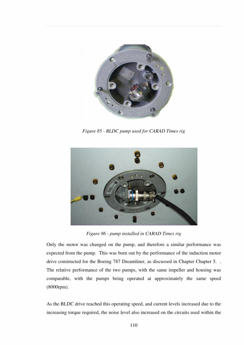
110
Figure 85 - BLDC pump used for CARAD Times rig
Figure 86 - pump installed in CARAD Times rig
Only the motor was changed on the pump, and therefore a similar performance was
expected from the pump. This was born out by the performance of the induction motor
drive constructed for the Boeing 787 Dreamliner, as discussed in Chapter Chapter 5. .
The relative performance of the two pumps, with the same impeller and housing was
comparable, with the pumps being operated at approximately the same speed
(8000rpm).
As the BLDC drive reached this operating speed, and current levels increased due to the
increasing torque required, the noise level also increased on the circuits used within the

111
drive. This was particularly noticeable on the reset pin of the DSP. This meant that
limited results were available at higher power, as the drive would reset itself once
operating speed was achieved. The pump used was the 8-pole BLDC. The speed
recorded in Figure 78 and Figure 79 (1875rpm) would represent a speed of 2500rpm if
used on a six pole machine (standard A380 BLDC pump motor).
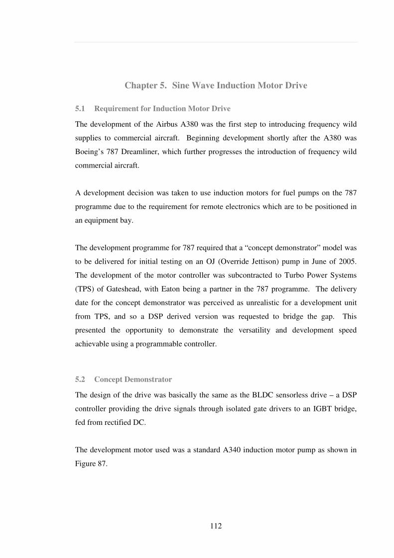
112
Chapter 5. Sine Wave Induction Motor Drive
5.1 Requirement for Induction Motor Drive
The development of the Airbus A380 was the first step to introducing frequency wild
supplies to commercial aircraft. Beginning development shortly after the A380 was
Boeing’s 787 Dreamliner, which further progresses the introduction of frequency wild
commercial aircraft.
A development decision was taken to use induction motors for fuel pumps on the 787
programme due to the requirement for remote electronics which are to be positioned in
an equipment bay.
The development programme for 787 required that a “concept demonstrator” model was
to be delivered for initial testing on an OJ (Override Jettison) pump in June of 2005.
The development of the motor controller was subcontracted to Turbo Power Systems
(TPS) of Gateshead, with Eaton being a partner in the 787 programme. The delivery
date for the concept demonstrator was perceived as unrealistic for a development unit
from TPS, and so a DSP derived version was requested to bridge the gap. This
presented the opportunity to demonstrate the versatility and development speed
achievable using a programmable controller.
5.2 Concept Demonstrator
The design of the drive was basically the same as the BLDC sensorless drive – a DSP
controller providing the drive signals through isolated gate drivers to an IGBT bridge,
fed from rectified DC.
The development motor used was a standard A340 induction motor pump as shown in
Figure 87.
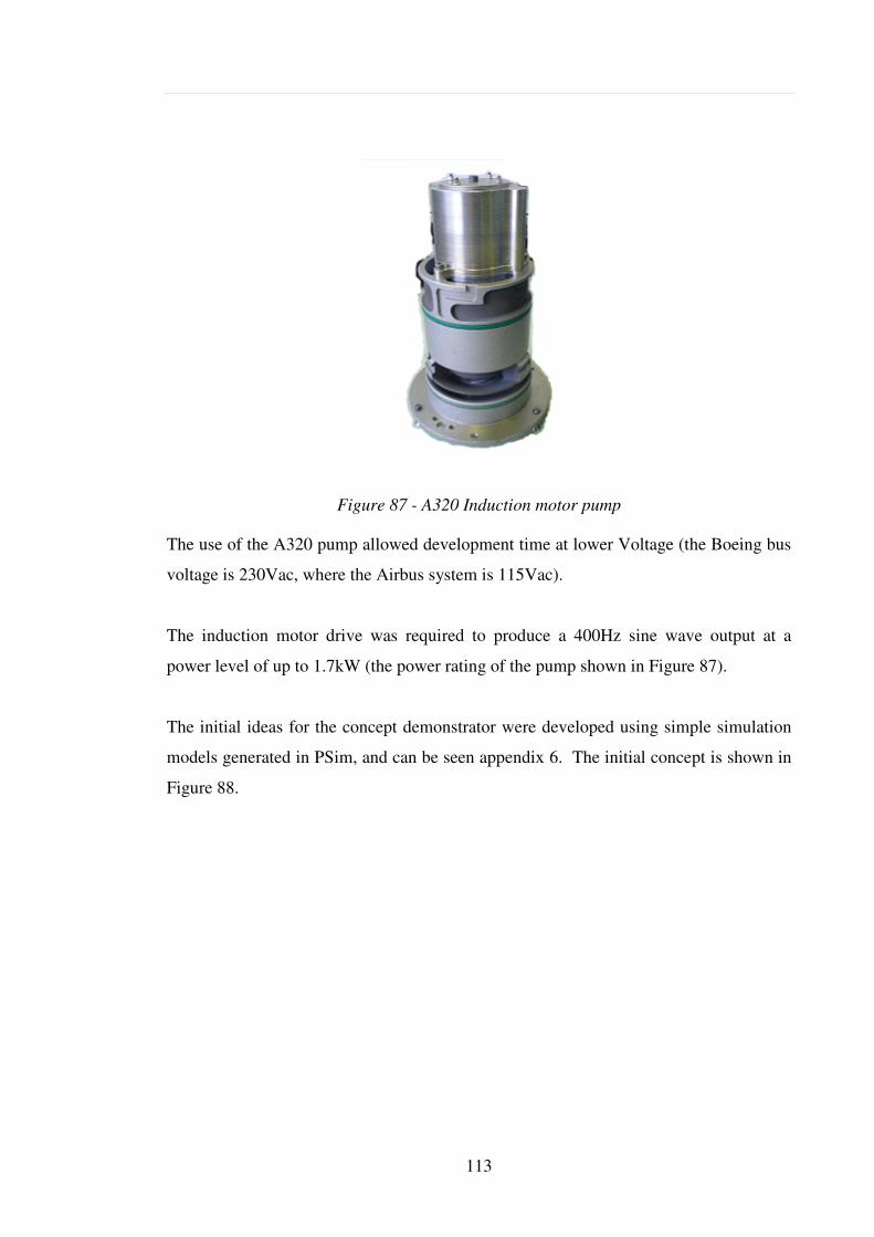
113
Figure 87 - A320 Induction motor pump
The use of the A320 pump allowed development time at lower Voltage (the Boeing bus
voltage is 230Vac, where the Airbus system is 115Vac).
The induction motor drive was required to produce a 400Hz sine wave output at a
power level of up to 1.7kW (the power rating of the pump shown in Figure 87).
The initial ideas for the concept demonstrator were developed using simple simulation
models generated in PSim, and can be seen appendix 6. The initial concept is shown in
Figure 88.
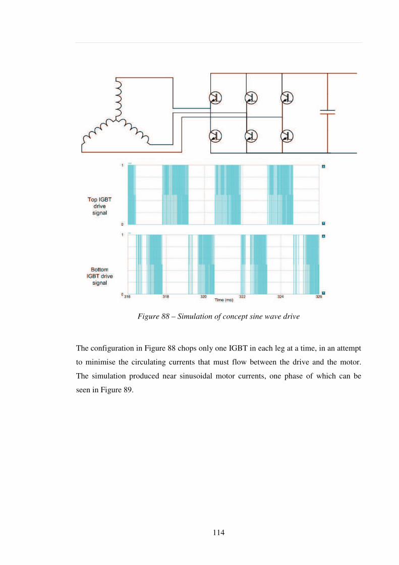
114
Figure 88 – Simulation of concept sine wave drive
The configuration in Figure 88 chops only one IGBT in each leg at a time, in an attempt
to minimise the circulating currents that must flow between the drive and the motor.
The simulation produced near sinusoidal motor currents, one phase of which can be
seen in Figure 89.
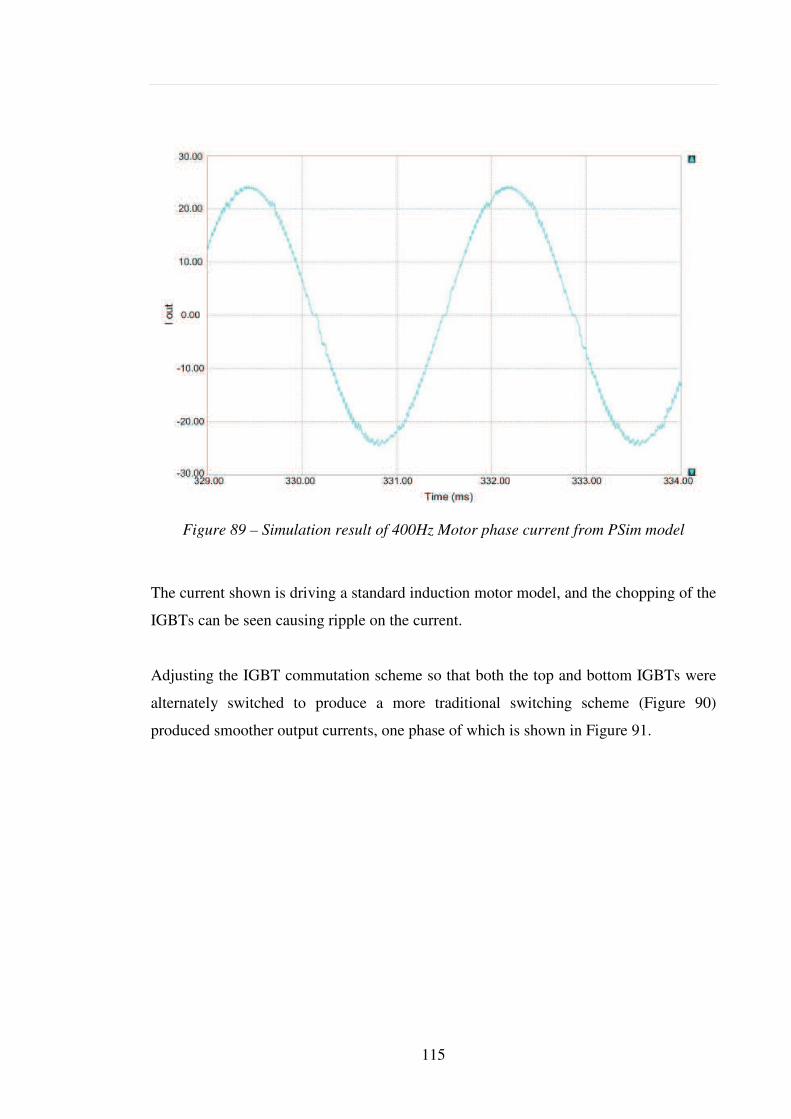
115
Figure 89 – Simulation result of 400Hz Motor phase current from PSim model
The current shown is driving a standard induction motor model, and the chopping of the
IGBTs can be seen causing ripple on the current.
Adjusting the IGBT commutation scheme so that both the top and bottom IGBTs were
alternately switched to produce a more traditional switching scheme (Figure 90)
produced smoother output currents, one phase of which is shown in Figure 91.
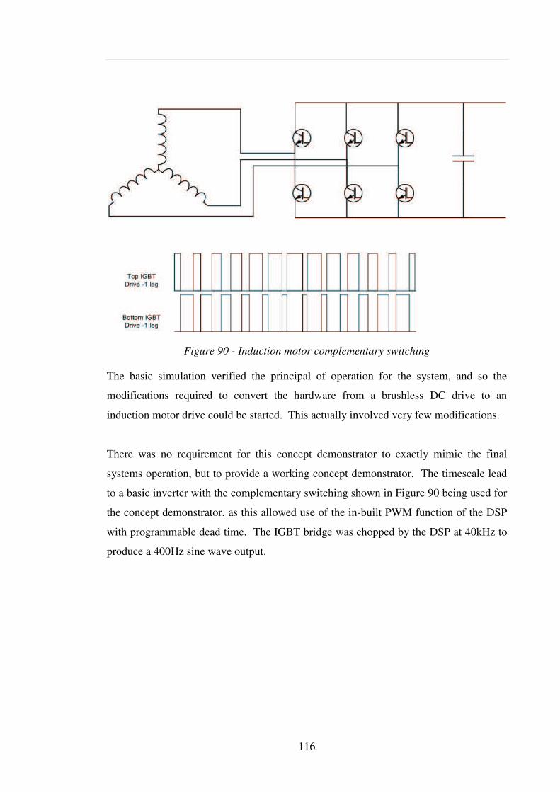
116
Figure 90 - Induction motor complementary switching
The basic simulation verified the principal of operation for the system, and so the
modifications required to convert the hardware from a brushless DC drive to an
induction motor drive could be started. This actually involved very few modifications.
There was no requirement for this concept demonstrator to exactly mimic the final
systems operation, but to provide a working concept demonstrator. The timescale lead
to a basic inverter with the complementary switching shown in Figure 90 being used for
the concept demonstrator, as this allowed use of the in-built PWM function of the DSP
with programmable dead time. The IGBT bridge was chopped by the DSP at 40kHz to
produce a 400Hz sine wave output.
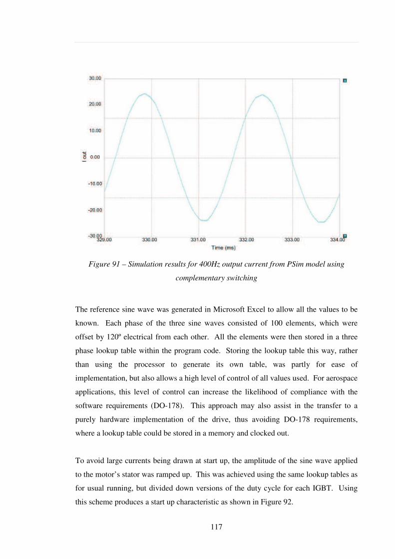
117
Figure 91 – Simulation results for 400Hz output current from PSim model using
complementary switching
The reference sine wave was generated in Microsoft Excel to allow all the values to be
known. Each phase of the three sine waves consisted of 100 elements, which were
offset by 120º electrical from each other. All the elements were then stored in a three
phase lookup table within the program code. Storing the lookup table this way, rather
than using the processor to generate its own table, was partly for ease of
implementation, but also allows a high level of control of all values used. For aerospace
applications, this level of control can increase the likelihood of compliance with the
software requirements (DO-178). This approach may also assist in the transfer to a
purely hardware implementation of the drive, thus avoiding DO-178 requirements,
where a lookup table could be stored in a memory and clocked out.
To avoid large currents being drawn at start up, the amplitude of the sine wave applied
to the motor’s stator was ramped up. This was achieved using the same lookup tables as
for usual running, but divided down versions of the duty cycle for each IGBT. Using
this scheme produces a start up characteristic as shown in Figure 92.
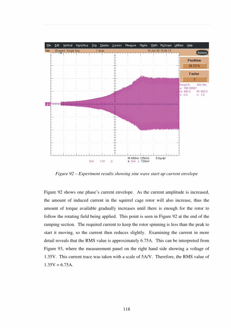
118
Figure 92 – Experiment results showing sine wave start up current envelope
Figure 92 shows one phase’s current envelope. As the current amplitude is increased,
the amount of induced current in the squirrel cage rotor will also increase, thus the
amount of torque available gradually increases until there is enough for the rotor to
follow the rotating field being applied. This point is seen in Figure 92 at the end of the
ramping section. The required current to keep the rotor spinning is less than the peak to
start it moving, so the current then reduces slightly. Examining the current in more
detail reveals that the RMS value is approximately 6.75A. This can be interpreted from
Figure 93, where the measurement panel on the right hand side showing a voltage of
1.35V. This current trace was taken with a scale of 5A/V. Therefore, the RMS value of
1.35V = 6.75A.
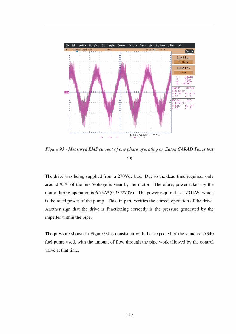
119
Figure 93 - Measured RMS current of one phase operating on Eaton CARAD Times test
rig
The drive was being supplied from a 270Vdc bus. Due to the dead time required, only
around 95% of the bus Voltage is seen by the motor. Therefore, power taken by the
motor during operation is 6.75A*(0.95*270V). The power required is 1.731kW, which
is the rated power of the pump. This, in part, verifies the correct operation of the drive.
Another sign that the drive is functioning correctly is the pressure generated by the
impeller within the pipe.
The pressure shown in Figure 94 is consistent with that expected of the standard A340
fuel pump used, with the amount of flow through the pipe work allowed by the control
valve at that time.
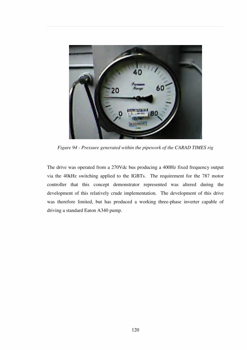
120
Figure 94 - Pressure generated within the pipework of the CARAD TIMES rig
The drive was operated from a 270Vdc bus producing a 400Hz fixed frequency output
via the 40kHz switching applied to the IGBTs. The requirement for the 787 motor
controller that this concept demonstrator represented was altered during the
development of this relatively crude implementation. The development of this drive
was therefore limited, but has produced a working three-phase inverter capable of
driving a standard Eaton A340 pump.
121
Chapter 6. Conclusions and Further Work
6.1 Conclusions
A sensorless BLDC motor controller has been constructed to operate at a fixed speed.
The use of a DSP controller has allowed rapid prototyping and experimentation to
implement a novel control scheme for the PWM current control. This allows fast
current switch off for both positive and negative going phase currents, which is not
normally achievable with a traditional chopped drive. The improved current switch off
is achieved by alternating the IGBT applying PWM to the winding.
A review of the possible sensorless techniques was undertaken (section Chapter 2. ),
and the Back EMF sensing technique chosen as the basis for the drive. The high level
of robustness of scheme compared to other sensorless techniques, and the proven
reliability within the aerospace industry of the technique means that the concept would
be a viable production solution and would prove easier to qualify for flight standard
hardware.
Converter topologies have been studied and analysed to ensure that the correct drive
configuration was being used for an aerospace converter. The extra control complexity
that the use of a more complex converter topology (such as a matrix converter)
requiring a complex, software based controller would increase the qualification
procedures required to gain acceptance by the aviation authorities, and would not be
suitable for the robust sensorless control scheme selected. The additional cost that this
would represent therefore becomes a driving factor in the assessment of each of the
control algorithms and converter topologies.
A novel use and expansion of an existing heating control scheme has been developed
using C code in a DSP and has allowed a stable drive operating with a 4µs interrupt
routine to be constructed. The Take Back Half control scheme has not previously been
well documented or researched, and has not been applied in the motor control field.
The application of it in a new area where the inherent stability of the controller is an
extremely desirable feature provides a novel use of this relatively simple controller.
122
The controller is generally used in relatively benign environments where slow response
times are not a hindrance, but has had to be adapted to the more dynamic requirements
of the motor drive. The expansion of the Take Back Half control scheme to create a
new and original implementation for motor control, the Take Back All controller,
improves the dynamic responsiveness of the controller but pushes the controller closer
to instability. A critical analysis of the potential phase error generated by the calculated
maximum deceleration that can be experienced by the pump, and implications on the
ability of the drive to cope with this was undertaken and showed that the averaging
required to maintain a stable system with the Take Back All control would impact the
controllers ability to actively control during maximum deceleration. The increase in
dynamic performance over a similarly averaged Take Back Half control algorithm has
been shown to be a desirable feature. The phase error generated has been shown to
decrease as the motor decelerates due to the counter based phase-locked loop
implemented digitally through the DSP.
The BEMF zero crossing detection technique has been implemented to produce a self
commutating motor drive, which then allows the speed control to be preformed by
simple current control. The simplification of the control, which for some aspects has
been implemented in purely hardware, has allowed a controller to be constructed that
could easily be translated in to a hardware only control scheme. The Eaton drive uses
an external current source to control the current applied to the motor, which in turn
controls the speed of the motor. The analysis of converter topologies, and the decision
to revert to a more traditional chopped bridge and remove the current source used in
Eaton’s production pump for this development was taken because of the increased
losses caused by its inclusion without any significant benefits. This increases the
possibility to use commercially available parts when the research presented here is used
in a commercial environment, thus keeping costs low.
Testing realised that the Take Back Half still required averaging to produce a truly
stable system, which increases the maximum phase error that the system would
experience. The algorithm has been expanded to make the response more dynamic by
increasing the amount of error used to correct the phase error. The ideal system would
allow all the error to be subtracted and an instant correction applied. As discussed, this
123
would produce a potentially unstable system, so an averaged version of the Take Back
All scheme has been implemented. The amount of averaging applied in the Take Back
All scheme takes the average over 1 electrical cycle to produce an averaged phase error.
The amount of averaging used (6 BEMF zero crossings) can be adjusted depending on
the dynamic response required for the system, and the maximum rate of deceleration.
The use of a DSP allowed development of the algorithm to produce a stable running
system at low power, but due to noise problems experienced at higher powers causing
the processor to reset the running was limited. This problem is discussed in Section 6.2
, Further Work.
Using virtually the same hardware as the BLDC drive a sine wave induction motor
drive has also been constructed, with limited development. This has shown the
flexibility and speed of implementation that a programmable controller would allow in
the development of future drives within Eaton and has lead to programmable controllers
being adopted by Eaton for drives currently under development. Again the complexity
of the drive was minimised, partly due to the limited development time, and partly to
allow a simplified hardware version to be implemented (should a production version be
required) which would only require qualification to DO-254, and remove the
requirement for DO-718 software qualification.
6.2 Further Work
Noise problems at high loads, and high speeds caused problems in operating the drive
towards its full capability. These are thought to be mainly due to the drive layout. The
main board was originally produced to allow the use of isolating amplifiers on the phase
inputs to the controller, which were subsequently removed due to issues with them as
described in section 3.18 . The inclusion of additional circuitry to allow an external
BEMF detector, providing a solution more geared towards hardware that would be
simpler to qualify, was not included on the original main board. Interfacing between
the original main board, and DSP daughter card was achieved using wire connections,
which are susceptible to noise pickup, and are one of the main contributors to the drive
not being able to run to its full capability.

124
A redesign on the main board layout removing all unnecessary circuitry and including
the additional circuitry, and improved connection between the DSP daughter card and
main board would undoubtedly improve the drive’s resilience to noise and allow higher
powers and speeds to be achieved from the controller. This would then allow more
dynamic testing of the controller, which would allow optimisation of the “Take Back
All” control algorithm, and possibly allow a reduction in the number of BEMF
detections that the controller averages. This would improve the dynamic response, and
reduce the possible phase error during maximum deceleration.
Eaton is currently funding an internal development programme for a “Next Generation
Motor Controller”, which will utilise a number of the concepts developed during this
thesis. The implementation of this drive is to be on an FPGA to remove software from
the system, and therefore the need for DO-178 qualification. This is being used as trial
development for a number of un-funded programmes that the company are bidding on,
and is likely to be implemented within the next three years as a flight certified
controller.
Section Chapter 3. contains a lot of simulation results for extreme cases of operation
and the theoretical ability of the drive to cope with these. Verification of the simulated
results is required from the physically implemented drive where possible to validate the
theory behind this implementation. These extreme operating conditions are generally
outside what is testable, occurring at temperatures beyond Eaton’s current test rigs
capabilities.
This work has not been published in papers or journals due to the industrial nature of
the project. Publication of the results gained here with appropriate credits will become
possible in the future, with Eaton’s agreement on any confidential information.
125
References
[1] A A AbdElhafez, A J Forsyth, A Review of More-Electric Aircraft, 13th
International Conference on Aerospace Sciences & Aviation Technology (ASAT-13),
May 26-28 2009.
[2] Ian Moir, Allan G Seabridge, Aircraft Systems: Mechanical, Electrical, and
Avionics Subsystem Integration, Wiley 2008, ISBN 978-0-470-05996-8.
[3] Airbus ABD100 Issue B, Table C, Power Quality Specification for 115Vac
systems.
[4] G Gong, U Drofenik and J W Kolar, 12-Pulse Rectifier for More Electric
Aircraft Applications, 2003 IEEE International Conference on Industrial Technology,
pp 1096 – 1101 Vol 2.
[5] Fairchild Semiconductor, ML4425 Sensorless BLDC Motor Controller Data
Sheet Rev. 1.0.2 7/2/01.
[6] Unitrode Products from Texas Instruments, UC1825/UC2825/UC3825 High
Speed PWM Controller Datatsheet, SLUS235A – March 1997 – Revised March 2004.
[7] Advanced Power Technology (APT), APT47N60BC3/APT47N60SC3 600V 47A
0.070 Super Junction MOSFET, 050-7144 Rev E, 4-2004.
[8] ABB Technical Guide No. 102, Effects of AC Drives on Motor Insulation, 1997
ABB Industrial Systems Inc.
[8] J.W. Finch, D. Giaouris, Controlled AC Electrical Drives, IEEE Transactions on
Industrial Electronics, Vol 55, No 2, February 2008.
126
[9] Li Ying and Nesimi Ertugrul, A Novel, Robust DSP-Based Indirect Rotor
Position Estimation for Permanent Magnet AC Motors Without Rotor Saliency, IEEE
Transactions on Power Electronics, Vol. 18, No. 2, March 2003.
[10] G. H. Jang, J. H. Park and J. H. Chang, Position detection and start-up algorithm
of a rotor in a sensorless BLDC motor utilising inductance, IEE Proc-Electr. Power
Appl. Vol 149, No 2, March 2002.
[11] G.Suresh, B.Fahimi, K . M . Rahman, M.Ehsani, Inductance Based Position
Encoding for Sensorless SRM Drives, IEEE Power Electronics Specialist Conference
1999, Vol 2, Pages 832 – 837.
[12] U.-H. Rieder M. Schroedl A. Ebner, Sensorless Control of an External Rotor
PMSM in the Whole Speed Range including Standstill using DC-link Measurements
only, 2004 35th Annual IEEE Power Electronics Specialists Conference, Aachen,
Germany.
[13] U.-H. Rieder, M. Schroedl, A Simulation Method for Analyzing Saliencies with
Respect to Enhanced INFORM-Capability for Sensorless Control of PM Motors in the
Low Speed Range including Standstill, IEEE 2005 European Conference on Power
Electronics and Applications .
[14] Tae-Hyung Kim, Byung-Kuk Lee, and Mehrdad Ehsani, Sensorless Control of
the BLDC Motors From Near Zero to High Speed, IEEE Applied Power Electronics
Conference and Exposition 2003, Vol 1, Pages 306 – 312.
[15] Hyunbae Kim, Kum-Kang Huh, Robert D Lorenz, and Thomas M Johns, A
Novel Method for Initial Rotor Position Estimation for IPM Synchronous Machine
Drives, IEEE Transactions of Industry Applications, Vol 40, No 5, September/October
2004.
127
[16] S. Nakashima, Y. Inagaki, I Miki, Sensorless Initial Rotor Position Estimation
of Surface Permanent-Magnet Synchronous Motor, IEEE Trans. Industrial Applications,
vol IA-36, pp. 1598-1603, Nov 2000.
[17] Paul P Acarnley and John F Watson, Review of Position Sensorless Operation of
Brushless Permanent Magnet Machines, IEEE Transactions on Industrial Electronics,
Vol 53, No 2, April 2006.
[18] Takashi Aihara, Akio Toba, Takao Yanase, Akihide Mashimo, Kenji Endo,
“Sensorless Torque Control of Salient-Pole Synchronous Motor at Zero-Speed
Operation”, IEEE Transactions on Power Electronics, Vol. 14, No.1, January 1999.
[19] Ji-Hoon Jang, Jung-Ik Ha, Motomichi Ohto, Kozo Ide, and Seung-Ki Sul,
Analysis of Permanent-Magnet Machine for Sensorless Control Based on High-
Frequency Signal Injection, IEEE Transactions on Industry Applications 2004, Vol 40,
Issue 6, Pages 1595 – 1604.
[20] Shigeo Morimoto, Masayuki Sanada, Yoji Takeda, Mechanical Sensorless
Drives of IPMSM With Online Parameter Identification, IEEE Transactions on Industry
Applications, Vol. 42, No. 5 September/October 2006.
[21] Marco Linke, Ralph Kennel, and Joachim Holtz, Sensorless position control of
Permanent Magnet Synchronous Machines without Limitation at Zero Speed, 28th
Annual Conference of the Industrial Electronics Society 2002, Vol 1, Pages 674 – 679.
[22] Marco Linke, Ralph Kennel, and Joachim Holtz, Sensorless Speed and Position
Control of Synchronous Machines using Alternating Carrier Injection, IEEE Electric
Machines and Drives Conference 2003, Vol 2, Pages 1211 – 1217.
[23] R Kennel, O. C. Ferreira, and P. Szczupak, “Parameter independent encoderless
control of servo drives without additional hardware components”, Bulletin of the Polish
Academy of Sciences.
128
[24] Sadayuki Sato, Hideaki Iura, Kozo Ide, Seung-Ki Sul, Three Years of Industrial
Experience with Sensorless IPMSM Drive based on High Frequency Injection Method,
2011 Symposium on Sensorless Control for Electrical Drives (SLED), 1 – 2 Sept 2011,
Pages 74 – 79.
[25] Dirk Paulus, Peter Landsmann, Ralph Kennel, Sensorless Field-Oriented
Control for Permanent Magnet Synchronous Machines with an Arbitrary Injection
Scheme and Direct Angle Calculation, 2011 Symposium on Sensorless Control for
Electrical Drives (SLED), 1 – 2 Sept 2011, Pages 41 – 46.
[26] T. Noguchi, K Yamada, S. Kondo, and I. Takahashi, Initial rotor position
estimation method of sensorless PM synchronous motor with no sensitivity to armature
resistance, IEEE Trans. Industrial Electronics, vol. IE-45, pp. 118-125, Jan. 1998.
[27] M.J. Corley and R.D. Lorenz, Rotor Position and velocity estimation for a
salient-pole permanent magnet synchronous motor at standstill and high speeds, IEEE
trans. Industrial Applications vol IA-34, pp. 784-789, July 1998.
[28] A.B. Kulkarni, and M. Ehsani, A novel position sensor elimination technique for
the interior permanent-magnet synchronous motor drive, IEEE Trans. Industrial
Applications, vol. IA-28, pp. 144-150, Jan. 1992.
[29] Vladan Petrovi, Aleksandar M. Stankovi, and Vladimir Blaško, Position
Estimation in Salient PM Synchronous Motors Based on PWM Excitation Transients,
IEEE Transactions on Industry Applications, Vol. 39, No. 3, May/June 2003.
[30] Tae-Hyung Kim, and Mehrdad Ehsani, Sensorless Control of the BLDC Motors
From Near-Zero to High Speeds, IEEE Transactions on Power Electronics, Vol 19, No
6, November 2004.
[31] Lennart Harnefors and Hans-Peter Nee, A General Algorithm for Speed and
Position Estimation of AC Motors, IEEE Transactions on Industrial Electronics, Vol 47,
No 1, February 2000.
129
[32] Bozo Terzic and Martin Jadric, Design and Implementation of the Extended
Kalman Filter for the Speed and Rotor Position Estimation of Brushless DC Motor,
IEEE Transactions on Industrial Electronics, Vol 48, No 6, December 2001.
[33] J. Hu, and B. Wu, New integration algorithms for estimating motor flux over a
wide speed range, IEEE Trans. Power Electronics, vol. PE-13, pp. 969-977, Sept. 1998.
[34] S. Grainger, M. Allan, Evaluation of A Hybrid Sensorless Position Observer for
Brushless DC Motors, IEEE European Conference on Power Electronics and
Applications 2005.
[35] Hsiu-Ping Wang and Yen-Tsan Liu, Integrated Design of Speed-Sensorless and
Adaptive Speed Controller for a Brushless DC Motor, IEEE Transactions on Power
Electronics, Vol. 21, No. 2, March 2006.
[36] Babak Nahid-Mobarakeh, Farid Meibody-Tabar, François-Michel Sargos,
Mechanical Sensorless Control of PMSM With Online Estimation of Stator Resistance,
IEEE Transactions on Industry Applications, Vol. 40, No. 2, March/April 2004.
[37] R. Wu, and G.R. Slemon, A permanent magnet motor drive without a shaft
sensor, IEEE Trans. Industrial Applications, vol. IA-27, pp. 1005-1011, Sept. 1991.
[38] T. Kosaka M. Fujitsuna T. Takahashi and N. Matsui, Current Polarity
Detection-based Simple Position Sensorless Drive of IPMSM for AC Compressor in
HEV, IEEE Industry Applications Conference 2004, Vol 1.
[39] Toshiyuki Murakami, Fangming Yu, and Kouhei Ohnishi, Torque Sensorless
Control in Multidegree-of-Freedom Manipulator, IEEE Transactions on Industrial
Electronics, Vol. 40, No. 2, April 1993.
[40] Todd D. Batzel, and Kwang Y. Lee, Electric Propulsion with Sensorless
Permanent Magnet Synchronous Motor: Implementation and Performance, IEEE
Transactions on Energy Conversion, Vol. 20, No. 3, September 2005.
130
[41] International Rectifier datasheet for IRMCK203, Data Sheet No. PD60225 Rev
B.
[42] S Grainger, M Allen, T Westwood, R Champaneri, Sensorless Control of a
Trapezoidal Brushless DC Motor Using the TMS320C25 DSP, Texas Instruments
Application Note SPRA323, ESIEE, Paris, September 1996.
[43] Jianwen Shao, Dennis Nolan, Maxime Teissier, and David Swanson, A Novel
Microcontroller-Based Sensorless Brushless DC (BLDC) Motor Drive for Automotive
Fuel Pumps, IEEE Transactions on Industry Applications, Vol 29, No 6,
November/December 2003.
[44] Kwang-Woon Lee, Dae-Kyong Kim, Tae-Duck Kim, and Jae-Young Choi,
Commutation Torque Ripple Reduction in a Position Sensorless Brushless DC Motor
Drive, 35th Annual IEEE Power Electronics Specialists Conference 2004.
[45] Kaushik Mukherjee, Sabyasachi SenGupta, Tapas Kumur Bhattacharya,
Sailendra N Bhadra, Ajit K Chattopadhyay, Sensorless Operation of a Thyristorized
Commutatorless Series Motor Drive, 2004 IEEE 25th Annual Power Electronics
Specialists Conference, 20 – 25 June 2004, Vol 1, Pages 458 – 463.
[46] Vincent Onde, Jianwen Shao, Shorten development cycle time and reduce
system cost when designing a brushless 3-phase motor control application, IEEE Power
Electronics and Motion Control Conference, 2004, Vol 3, Pages 1298 – 1305.
[47] Jianwen Shao, Dennis Nolan, Further Improvement of Direct Back EMF
Detection for Sensorless Brushless DC (BLDC) Motor Drives, IEEE Applied Power
Electronics Conference and Exposition, 2005, Vol 2, pages 933 – 937.
[48] Genfu Zhou, Zhigan Wu, Jianping Ying , Unattenuated BEMF Detection for
Sensorless Brushless DC (BLDC) Motor Drives, IEEE Power Electronics and Motion
Conference, 2004. Vol 3, Pages 1292 – 1297.
131
[49] Kuang-Yao Cheng, and Ying-Yu Tzou, Design of a Sensorless Commutation IC
for BLDC Motors, IEEE Transactions on Power Electronics, Vol. 18, No. 6, November
2003.
[50] Jianwen Shao, Dennis Nolan, Thomas Hopkins, Improved Direct Back EMF
Detection for Sensorless Brushless DC (BLDC) Motor Drives, IEEE Applied Power
Electronics Conference and Exposition, 2003, Vol 1, Pages 300 – 305.
[51] Jun-ichi Itoh, Naofumi Nomura, Hiroshi Ohsawa, “A Comparison between V/f
Control and Position-Sensorless Vector Control for the Permanent Magnet
Synchronous Motor, IEEE Power Conversion Conference, 2002, Vol 3, Pages 1310 –
1315.
[52] Doo-Hee Jung and In-Joong Ha, Low-Cost Sensorless Control of Brushless DC
Motors Using a Frequency-Independent Phase Shifter, IEEE Transactions on Power
Electronics, Vol. 15, No. 4, July 2000.
[53] Tae-Hyung Kim, Hyung-Woo Lee, and Mehrdad Ehsani, State of the Art and
Future Trends in Position Sensorless Brushless DC Motor/Generator Drives, IEEE
Industry Electronics Society 2005.
[54] Byoung-Gun Park, Tae-Sung Kim, Ji-Su Ryu, Dong-Seok Hyun, Fuzzy Back-
EMF Observer for Improving Performance of Sensorless Brushless DC Motor Drive,
Twenty-First Annual IEEE Applied Power Electronics Conference and Exposition
2006.
[55] Cheng-Tsung Lin, Chung-Wen Hung, and Chih-Wen Liu, Sensorless Control
for Four-Switch Three-Phase Brushless DC Motor Drives, IEEE Industry Applications
Conference 2006, Vol 4, Pages 2048 – 2053.
132
[56] Luiz A. de S. Ribeiro, Michael C. Harke, Robert D. Lorenz, Dynamic Properties
of Back-emf Based Sensorless Drives, IEEE Industry Applications Conference 2006,
Vol 4, Pages 2026 – 2033.
[57] Sensorless BLDC Motor Control on MC68HC908MR32, Freescale
Semiconductor Application note AN2355/D 11/2002.
[58] Juan Dixon, Matías Rodríguez and Rodrigo Huerta, POSITION ESTIMATOR
AND SIMPLIFIED CURRENT CONTROL STRATEGY FOR BRUSHLESS-DC
MOTORS, USING DSP TECHNOLOGY, 28th Annual Conference of the Industrial
Electronics Society 2002, Vol 1, Pages 590 -596.
[59] Jianwen Shao, “Direct Back EMF Detection for Sensorless Brushless DC
(BLDC) Motor Drives”, Master of Science in Electrical Engineering Thesis.
[60] M Tursini, C Olivieri, L Di Leonardo, Analysis of phase-detection algorithms
for back-EMF-based sensorless strategies through real-time simulations, 2011
Symposium on Sensorless Control for Electric Drives (SLED), 1 – 2 Sept 2011, Pages
129 – 137.
[61] RTCA, DO-254 Design Assurance Guidance for Airborne Electronic Hardware,
April 19, 2000, Prepared by RTCA SC-180.
[62] RTCA, DO-178B Software Considerations in Airborne Systems and Equipment
Certification, December 1, 1992, Prepared by RTCA SC-167, EUROCAE WG-12.
[63] G El-Murr, D Giaouris, J.W. Finch, Totally Parameter Independent Speed
Estimation of Synchronous Machines Based on Online Short Time Fourier Transform
Ridges, Engineering Letters, 16:1, EL_16_1_14.
[64] Nicola Bianchi, Silverio Bolognani, Fabio Luke, High Speed Drive Using a
Slotless PM Motor, 2004 IEEE 35th Annual Power Electronics Specialists Conference
20 – 25 June 2004, Vol 1, pages 458 – 463.
133
[65] Nikolas Teske, Greg M. Asher, Keith J. Bradley, Mark Sumner, Analysis and
Suppression of Inverter Clamping Saliency in Sensorless Position Controlled Induction
Machine Drives, IEEE Industry Applications Conference 2001, Vol 4, Pages 2629 –
2636.
[66] Jordi Català i López, Luis Romeral, Antoni Arias, Emiliano Aldabas, “Novel
Fuzzy Adaptive Sensorless Induction Motor Drive”, IEEE Transactions on Industrial
Electronics, Vol. 53, No. 4, August 2006.
[67] B. Fahimi, M. Ehsanil, G. Suresh, “Review of Sensorless Control Methods in
Switched Reluctance Motor Drives, IEEE Industry Applications Conference, 2000, Vol
3, Pages 1850 – 1857.
[68] Kazuhiro Ohyama, Greg M. Asher, Mark Sumner, Comparative Analysis of
Experimental Performance and Stability of Sensorless Induction Motor Drives, IEEE
Transactions on Industrial Electronics, Vol. 53, No. 1, February 2006.
[69] G.Suresh, B.Fahimi, K.M.Rahman, M.Ehsani, I.Panahi, our-quadrant Sensorless
SRM Drive with High Accuracy at All Speeds, IEEE Applied Power Electronics
Conference and Exposition 1999, Vol 2, Pages 1226 – 1231.
[70] G.Suresh, K.M.Rahman, B.Fahimi, M.Ehsani, Self-tuning Sensorless SRM
Drives for Low Cost Mass Production, The 1998 IEEE Industry Applications
Conference, Vol 1, Pages 593 – 600.
[71] Akitoshi Iwata, Shinji Ichikawa, Shigeru Okuma, Mutuwo Tomitat, Shinji
Dokit, Position and velocity sensorless control of SynRMs using on-line parameter
identification, IEEE Industrial Electronics Society 2003, Vol 3, Pages 2156 – 2161.
[72] Radim Visinka, 3-Phase Switched Reluctance (SR) Sensorless Motor Control
Using a 56F80x, 56F8100 or 56F8300 Device, Design of a Motor Control Application,
Freescale Semiconductor, Application Note AN1932, Rev. 2, 2/2005.
134
[73] Shinji Ichikawa, Mutuwo Tomita, Shinji Doki, and Shigeru Okuma, Sensorless
Control of Synchronous Reluctance Motors Based on Extended EMF Models
Considering Magnetic Saturation With Online Parameter Identification, IEEE
Transactions on Industry Applications, Vol 42, No. 5, September/October 2006.
[74] Jiri Lettl and Stanislav FLigl, “Matrix Converter Control System”, Progress In
Electromagnetics Research Symposium 2005, Hangshou, China, August 22-26.
[75] S Khwan-on, L De Lillo, L Empringham, P W Wheeler, A Fault Tolerant Matrix
Converter Motor Drive under Open Phase Faults, 5th IET International Conference on
Power Electronics, Machines and Drives (PEMD 2010), 19 – 21 April 2010, Pages 1 –
6.
[76] René Vargas, Ulrich Ammann, José Rodríguez, Predictive Approach to Increase
Efficiency and Reduced Switching Losses on Matrix Converters, IEEE Transactions on
Power Electronics, Vol 24, No 4, April 2009.
[74] Pat Wheeler, Jon Claire, Liliana de Lillo, Keith Bradley, Martin Aten, Chris
Whitley, Graham Towers, A Reliability Comparison of a Matrix Converter and an 18-
Pulse Rectifier for Aerospace Applications, 12th International Power Electronics and
Motion Control Conference, 2006 (EPE-PEMC 2006), Aug 30 – Sept 1 2006, Pages
496 – 500.
[78] Lixiang Wei, T.A.Lipo and Ho Chan, Matrix Converter Topologies With
Reduced Number of Switches, IEEE 33rd Annual Power Electronics Specialists
Conference 2002, Vol 1, Pages 57 – 63.
[79] Texas Instruments, TMS320F2812 eZdsp Start Kit (DSK) development kit
datasheet, www.ti.com
[80] Dr Martin Dentan, Introduction to Radiation Effects on Electronic Components
and Circuits, EFDA-JET Close Support Unit, 23 March 2006.
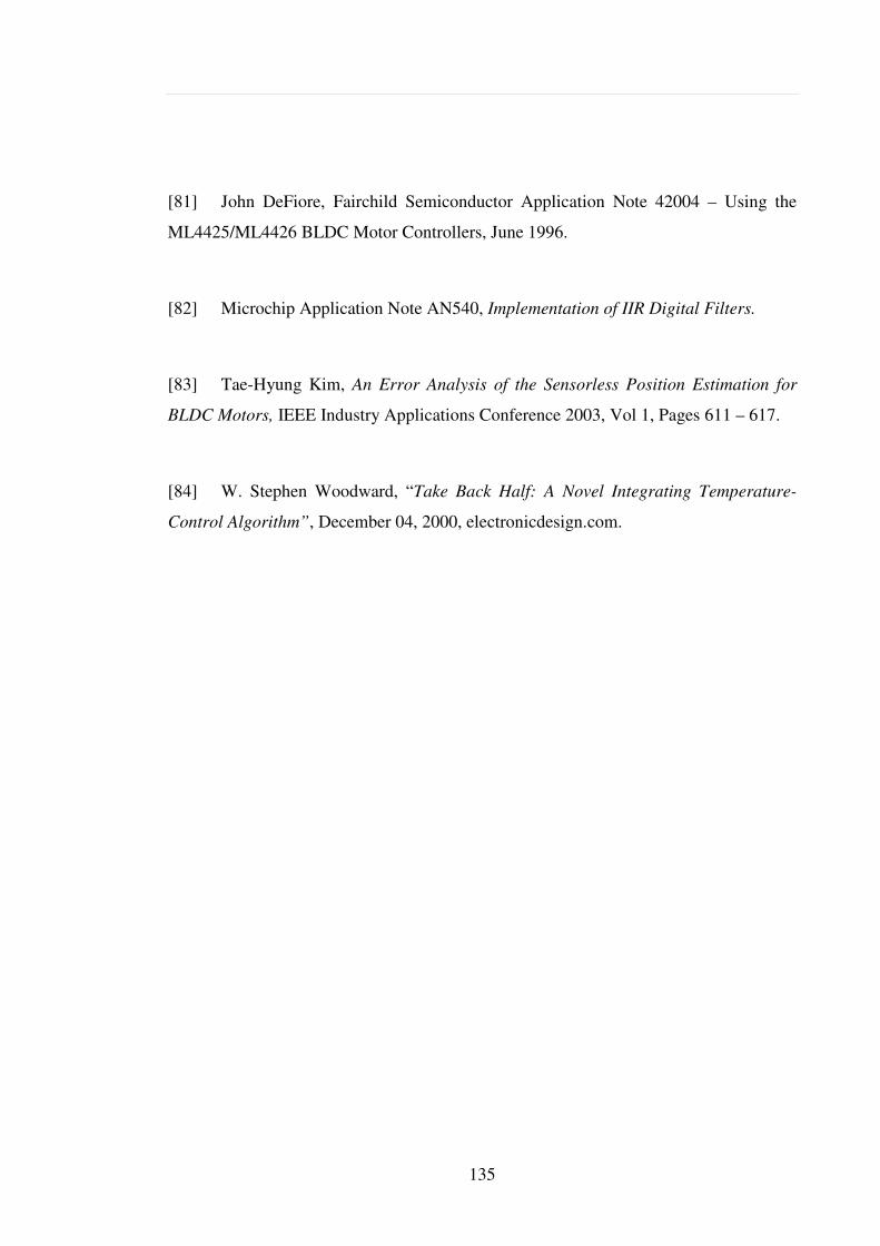
135
[81] John DeFiore, Fairchild Semiconductor Application Note 42004 – Using the
ML4425/ML4426 BLDC Motor Controllers, June 1996.
[82] Microchip Application Note AN540, Implementation of IIR Digital Filters.
[83] Tae-Hyung Kim, An Error Analysis of the Sensorless Position Estimation for
BLDC Motors, IEEE Industry Applications Conference 2003, Vol 1, Pages 611 – 617.
[84] W. Stephen Woodward, “Take Back Half: A Novel Integrating Temperature-
Control Algorithm”, December 04, 2000, electronicdesign.com.

136
Abbreviations and symbols used
BEMF – Back Electro Motive Force – The induced voltage in the windings due to the
magnetic field of the rotor.
PLL – Phase-Locked Loop
VCO – Voltage Controlled Oscillator
DSP – Digital Signal Processor
ML4425 – Fairchild Sensorless Brushless DC motor controller
IGBT – Insulated Gate Bipolar Transistor
4046 – HEF4046 PLL IC
– phi - phase
- delta – difference in
- pi – 3.14159
– alpha – is proportional to
– omega – rotational frequency
BLDC - Brushless Direct Current

137
Appendix A. Motor Details

138
Permanent Magnet Machine Record
Reference no FPA380demoB
Winding W18-3-001 Star Stator Lamination 501-2-15219
Lamination
Material
M300-35 Rotor Assembly BLDC25
Wire Size 0.4mm Wires in Hand 2
Turns Per Coil 28 Parallel Paths 3
CSA One Turn 0.2513 sqmm Turns/phase 56
Slot Insulation N/K/N (2/2/2) Copper Area 38.8 sqmm
Slot Fill 62.2% Slots Skewed 1
End Turn OD 54 mm Stack Length 52 mm
End Turn Length 15 mm Stacking Factor 0.98 pu
Stator ID 35 mm Radial Airgap 2 mm
Stator DSO 0.4
Frame Material Aluminium Cast Frame OD 70 mm
Comments: A380 demo pump motor to provide 3kW (2.49Nm @ 11500rpm) 170Vdc

139
Stator Lamination Record
Reference No 501-2-15219
Outside Diameter 58 mm Slot Die Ref. 501-2-15219
Inside Diameter 35 mm No Slots 18
Core Inside Dia. 52 mm Lamination Thickness 0.35 mm
Width Tooth Mean 2.215 mm Slot Opening Depth 0.4 mm
Outer Dia. 2.199 mm Slot Opening Breaks Out 0.1 mm
Inner Dia. 2.247 mm
Comments: Size 25 brushless motor lam
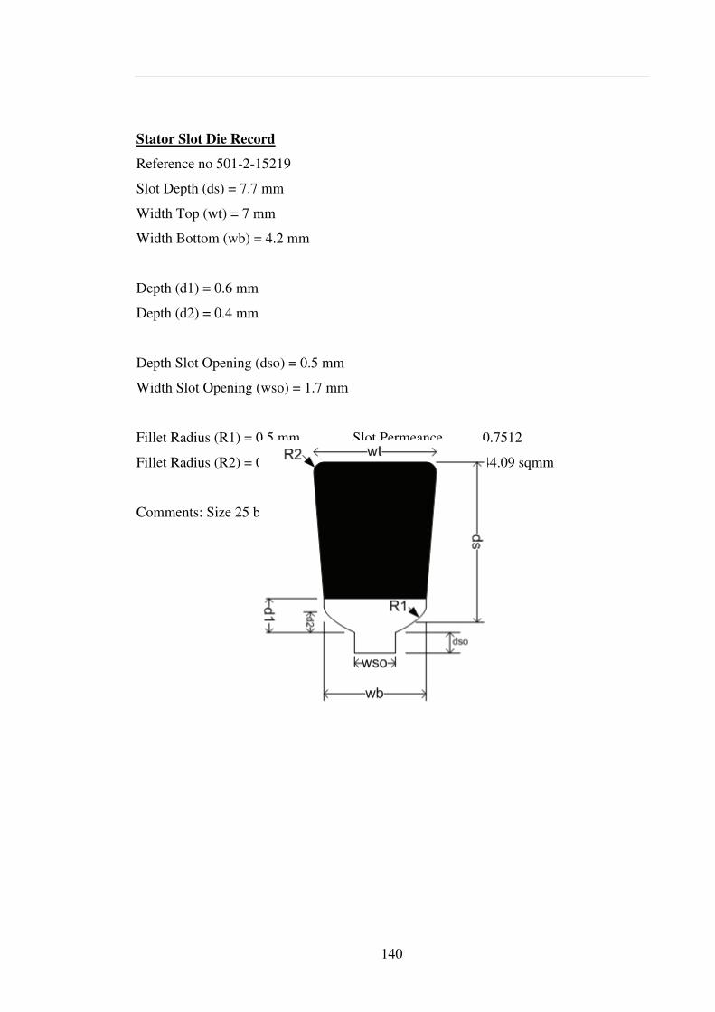
140
Stator Slot Die Record
Reference no 501-2-15219
Slot Depth (ds) = 7.7 mm
Width Top (wt) = 7 mm
Width Bottom (wb) = 4.2 mm
Depth (d1) = 0.6 mm
Depth (d2) = 0.4 mm
Depth Slot Opening (dso) = 0.5 mm
Width Slot Opening (wso) = 1.7 mm
Fillet Radius (R1) = 0.5 mm Slot Permeance 0.7512
Fillet Radius (R2) = 0.5 mm Slot Area 44.09 sqmm
Comments: Size 25 brushless motor lam

141
Permanent Magnet Rotor Record
Reference No BLDC25
Magnet Outside Dia. 31 mm
Magnet Material Recoma 28
Magnet Min. Length 3.32 mm
Magnet Avg. Length 4.106 mm
Magnet Max. length 4.5 mm
Pole Pair 3
Pole Arc/Pole Pitch 0.75
Magnet Side Clearance 0.4193 mm
Magnet Angle 0 mm
Sleeve Outside Dia. 32 mm
Sleeve Material Titanium 6A14V
Hub Across Flats 22 mm
Hub Material Stainless S80
Hub Inside Dia. 12 mm
No Shaft Fitted (rotor hub is used as shaft)
Comments: Size 25 brushless motor

142
3 Phase Winding Record
Reference No W18-3-001
Layer No. 2 Slot No. 18
Pole Pairs 3 Coil Pitch 1
Phase Spread 60 MMF Factor 1.5107
Winding Factors kw1 = 1
kw3 = 1 kw5 = 1
kw7 = 1 kw 9 = 1
kw11 = 1 kw13 = 1
Winding Layout
1 2 3 4 5 6 7 8 9 10 11 12 13 14 15 16 17 18
+R -B +Y -R +B -Y +R -B +Y -R +B -Y +R -B +Y -R +B -Y
+R -B +Y -R +B -Y +R -B +Y -R +B -Y +R -B +Y -R +B -Y
Comments: Constant full pitch winding

143
Lamination Material Record
Reference No M300-35
Density 7.6 gm/cm^3 Conductivity 28 W/m.deg C
Modulus Elasticity 200GPa Poissons Ratio 0.29
-100 deg C 0 deg C 100 deg C 200 deg C
Expansion Coeff (mm/mm.deg C) 1.22E-5 1.22E-5 1.22E-5 1.22E-5
Compressive Yield (MPa) 370 370 370 370
Tensile Yield (MPa) 370 370 370 370
Comments: EN 10106 Silicon Steel
BH Curve Data
B(T) H(A/m) B(T) H(A/m)
0.000 0.0 1.5 1630
0.4 42 1.6 3460 Resistivity 0.5 uohm.m
0.5 51 1.7 6540 Hysteresis Constant 0.025
0.6 62 1.8 11600 Hysteresis Power 1.8
0.7 77 1.9 19600
0.8 97 2 31600
0.9 124 2.1 50200
1 158
1.1 208
1.2 282
1. 3 406
1.4 698
BH Curve Cubic Spline Equations
0.0 to 0.4
Sqrt(H)= 16.2019*B
0.4 to 0.9

144
Sqrt(H)= 4.4002 +5.32312*B +-2.46851*B^2 +5.41016*B^3
0.9 to 1.2
Sqrt(H)= 0.521673 +24.5176*B +-29.1572*B^2 +16.6878*B^3
1.2 to 1.5
Sqrt(H)= -1532.38 +3691.77*B +-2954.6*B^2 +794.943*B^3
1.5 to 1.8
Sqrt(H)= -609.837 +1140.71*B +-767.626*B^2 +197.422*B^3
1.8 to 2.1
Sqrt(H)= -3025.56 +4827.22*B +-2632.32*B^2 +509.767*B^3

145
Permanent Magnet Material Record
Reference No Recoma 28
Remanence (Brem) 1.07 T Remanence Coeff -0.00035/deg C
Intrinsic Coercivity (Hci) 2000kA/m Intrinsic Coercivity Coeff -0.002/deg C
Relative Recoil Permeability 1.06 Resistivity 0.9 uohm.cm
Density 8.3 gm/cm^3 Conductivity 10 W/m.deg C
Modulus Elasticity 210 GPa Poissons Ratio 0.3
-100 deg C 0 deg C 100 deg C 200 deg C
Expansion Coeff (mm/mm.deg C) 8.1E-6 8.1E-6 8.1E-6 8.1E-6
Compressive Yield (MPa) 600 600 600 600
Comments: Sm2-Co17 Typical values at 20C Max use 250C

146
Shaft/Frame Material Record
Reference No Stainless S80
Density 7.72 gm/cm^3 Conductivity 16 W/m.deg C
Modulus Elasticity 193 GPa Poissons Ratio 0.3
-100 deg C 0 deg C 100 deg C 200 deg C
Expansion Coeff (mm/mm.deg C) 1E-5 1E-5 1E-5 1E-5
Compressive Yield (MPa) 700 700 700 700
Tensile Yield (MPa) 700 700 700 700
Comments: S80 magnetic stainless – 431S29
BH Curve Data
B(T) H(A/m) B(T) H(A/m)
0.000 0.0 1.5 80000
0.4 640
0.5 736
0.6 832
0.7 944
0.8 1104
0.9 1312
1 1600
1.1 2080
1.2 2960
1. 3 4400
1.4 10400
BH Curve Cubic Spline Equations
0.0 to 0.4
Sqrt(H) = 63.2456*B
0.4 to 0.9

147
Sqrt(H)=14.4346 +41.2931*B +-48.4163*B^2 +32.7028*B^3
0.9 to 1.2
Sqrt(H)=-140.442 +543.445*B +-590.217*B^2 +227.215*B^3
1.2 to 1.5
Sqrt(H)=-42462 +99613.3*B +-77784.5*B^2 +20248.9*B^3

148
Appendix B. IGBT Gate Drive Circuit
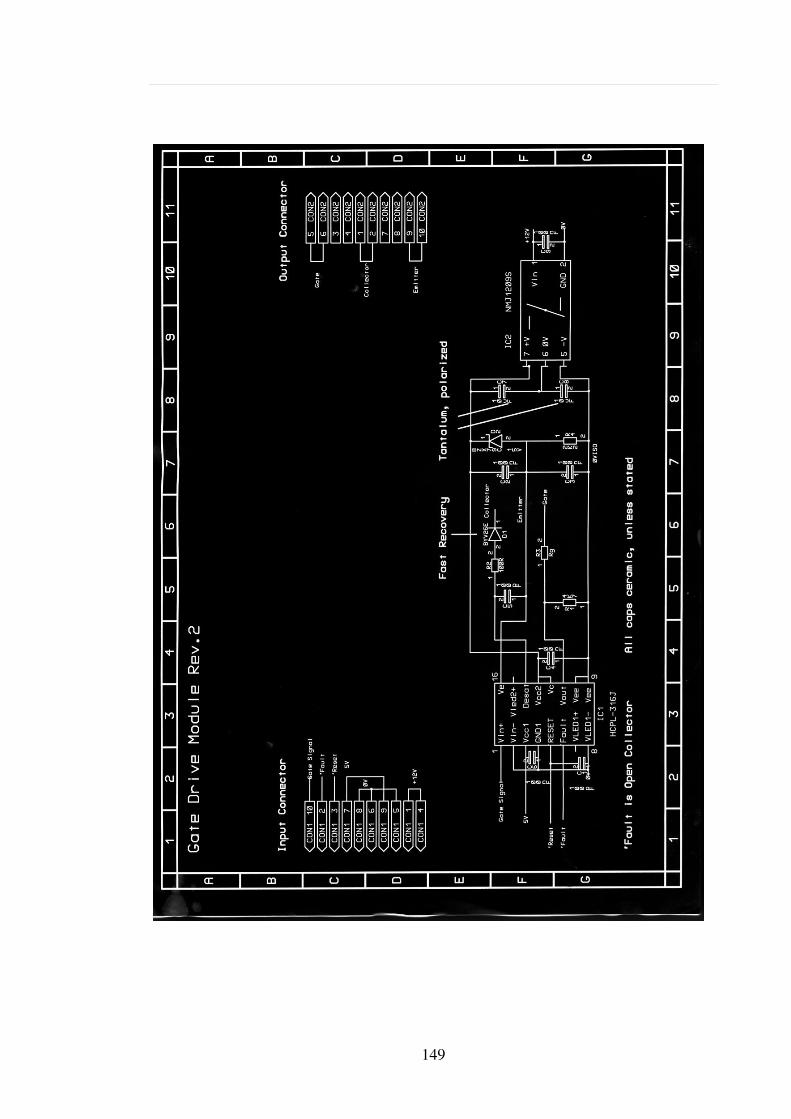
149

150
Appendix C. Flow Charts for Sinewave Induction Motor Drive
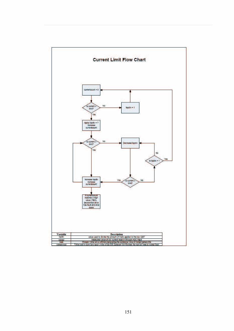
151
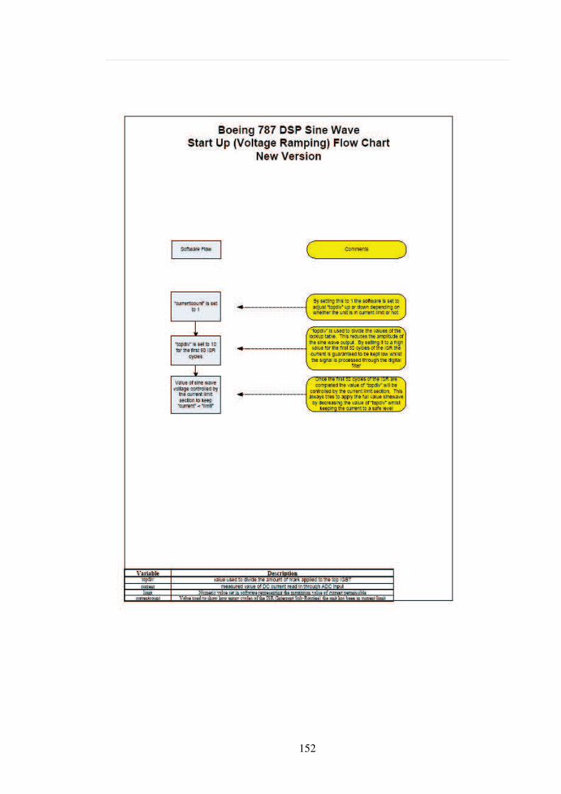
152
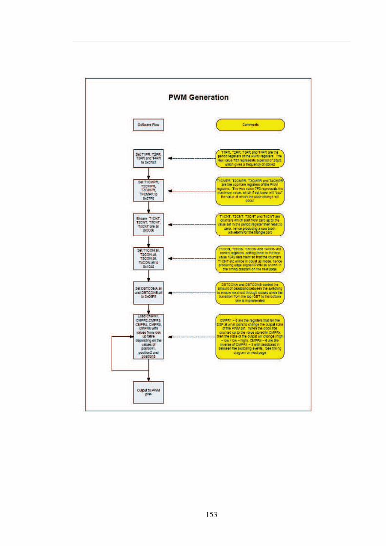
153
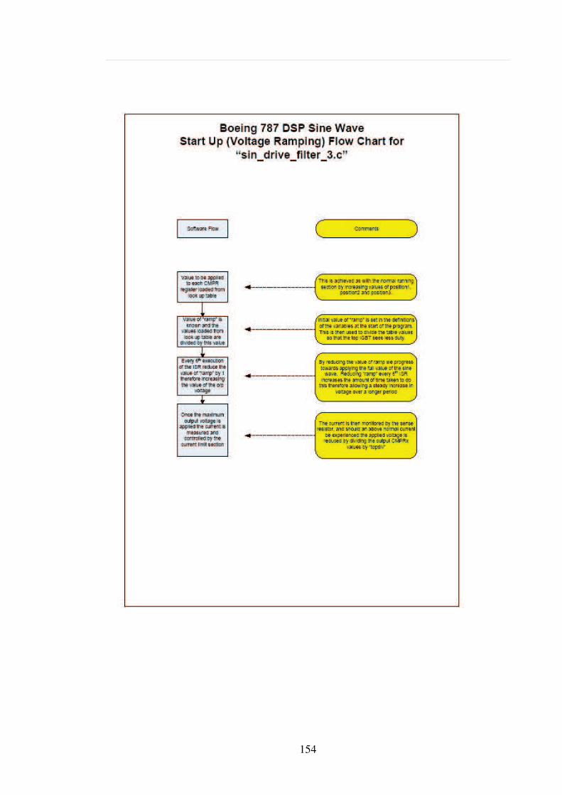
154
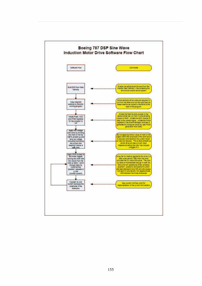
155

156
Appendix D. Circuit Diagrams

157
This page to be substituted for A3 sheet showing full circuit diagram (attached file)

158
Appendix E. Saber Simulation
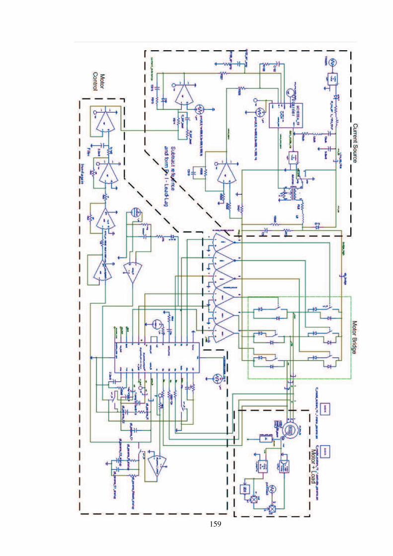
159
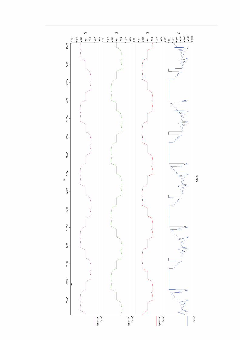
160

161
Appendix F. PSim Simulations
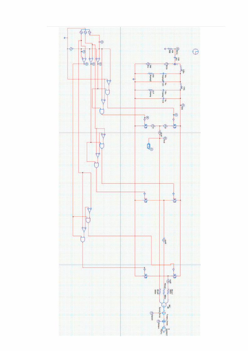
162
Appendix G.
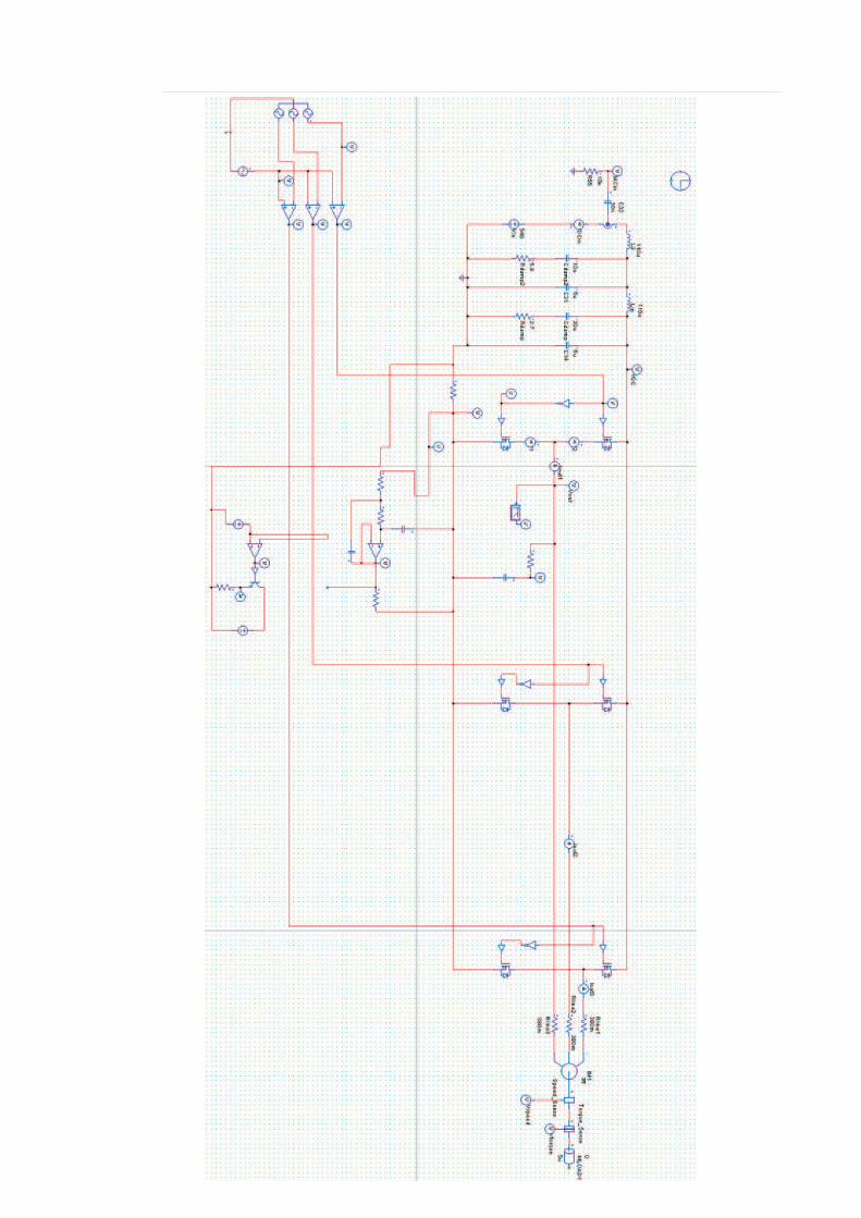
163

164
HEF4046 PLL Datasheet
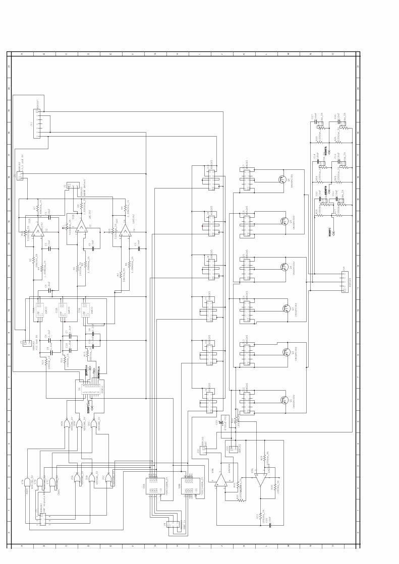
0 0
1 1
2 2
3 3
4 4
5 5
6 6
7 7
8 8
9 9
10
10
11
11
12
12
13
13
14
14
15
15
16
16
17
17
18
18
19
19
20
20
21
21
AA
BB
CC
DD
EE
FF
GG
HH
II
JJ
KK
LL
MM
NN
OO
U1A
lm833
1op
1-
1+
1v+
1v-
U1B
lm833
2OP
2-
2+
2v+
2v-
R1
24kOhm_5%
R2
24kOhm_5%
U2A
LM139J
5 4
3
2
12
U2B
LM139J
7 6
3
1
12
U2C
LM139J
9 8
3
14
12
U3A
lm833
1op
1-
1+
1v+
1v-
R3
24kOhm_5%R4
1.00MOhm_1%
R5
1.00MOhm_1%
R6
1.00MOhm_1%
C1
15nF
C2
15nF
C3
15nF
R7
1.00kOhm_1%
R8
1.00kOhm_1%
R9
1.00kOhm_1%
C4
10nF
C5
10nF
J2
HDR1X3
BEMF detect
R10
510kOhm_5%
R11
510kOhm_5%
R12
510kOhm_5%
J3
HDR1X2
+12 and 0V
J1
HDR1X2
+3.3 and 0V
C6
2.2nF
C7
2.2nF
C8
2.2nF
C9
1.0nF
C10
1.0nF
C11
1.0nF
R13
100Ohm_1%
R14
100Ohm_1%
R15
100Ohm_1%
U4
DG411
1 2 3 4 5 6 7 8
910
11
12
13
14
15
16
U5A
4001BD_5V
U5B
4001BD_5V
U5C
4001BD_5V
U6A
4001BD_5V
U6B
4001BD_5V
U6C
4001BD_5V
U7A
4081BD_5V
U7B
4081BD_5V
U7C
4081BD_5V
J5
HDR2X3
DSP signals
J4
HDR2X3
PWM in
U8A
74HC244DW_2V
1Y1
18
1Y2
16
1Y3
14
1Y4
12
1A1
2
1A2
4
1A3
6
1A4
8
~1G
1
U8B
74HC244DW_2V
2Y1
9
2Y2
7
2Y3
5
2Y4
3
2A1
11
2A2
13
2A3
15
2A4
17
~2G
19
Abot
Bbot
Cbot
12
3
56
4
CA
B
J6
HDR2X5
J12
HDR2X5
J13
HDR2X5
J14
HDR2X5
J15
HDR2X5
J16
HDR2X5
J17
HDR2X5
J18
HDR1X5
J19
HDR1X2
J20
HDR2X5
J7
HDR2X5
J8
HDR2X5
J9
HDR2X5
J10
HDR2X5
J11
HDR1X7
R22
100Ohm_5%
R16
100Ohm_5%
R17
100Ohm_5%
R18
100Ohm_5%
R19
100Ohm_5%
R20
100Ohm_5%
R21
100Ohm_5%
C12
10nF
R23
100Ohm_5%
C13
10nF
R24
100Ohm_5%
C14
10nF
R25
100Ohm_5%
C15
10nF
R26
100Ohm_5%
C16
10nF
R27
100Ohm_5%
C17
10nF
R28
100Ohm_5%
U9A
LM258N
3 2
48
1R29
100Ohm_5%
R30
100Ohm_5%
R31
100Ohm_5%R32
100Ohm_5%
U9B
LM258N
5 6
48
7
R33
100Ohm_5%
C18
10nF
J21
HDR1X2
ADC
BEMFC
BEMFB
BEMFA
BEMFCin
BEMBin
BEMFAin
C19
4700uF-POL
Q1
IRG4PC30U
Q2
IRG4PC30U
Q3
IRG4PC30U
Q4
IRG4PC30U
Q6
IRG4PC30U
Q5
IRG4PC30U

DATA SHEET
Product specification
File under Integrated Circuits, IC04
January 1995
INTEGRATED CIRCUITS
HEF4046BMSIPhase-locked loop
For a complete data sheet, please also download:
• The IC04 LOCMOS HE4000B LogicFamily Specifications HEF, HEC
• The IC04 LOCMOS HE4000B LogicPackage Outlines/Information HEF, HEC
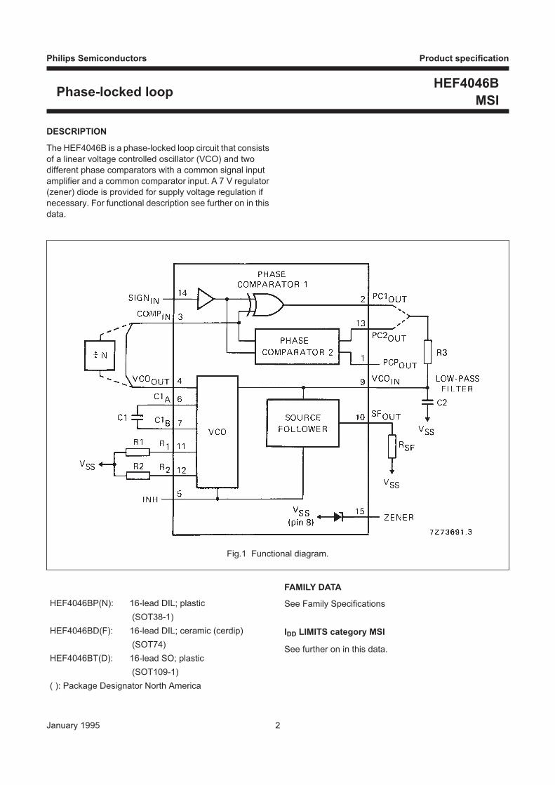
January 1995 2
Philips Semiconductors Product specification
Phase-locked loopHEF4046B
MSI
DESCRIPTION
The HEF4046B is a phase-locked loop circuit that consists
of a linear voltage controlled oscillator (VCO) and two
different phase comparators with a common signal input
amplifier and a common comparator input. A 7 V regulator
(zener) diode is provided for supply voltage regulation if
necessary. For functional description see further on in this
data.
Fig.1 Functional diagram.
HEF4046BP(N): 16-lead DIL; plastic
(SOT38-1)
HEF4046BD(F): 16-lead DIL; ceramic (cerdip)
(SOT74)
HEF4046BT(D): 16-lead SO; plastic
(SOT109-1)
( ): Package Designator North America
FAMILY DATA
See Family Specifications
IDD LIMITS category MSI
See further on in this data.
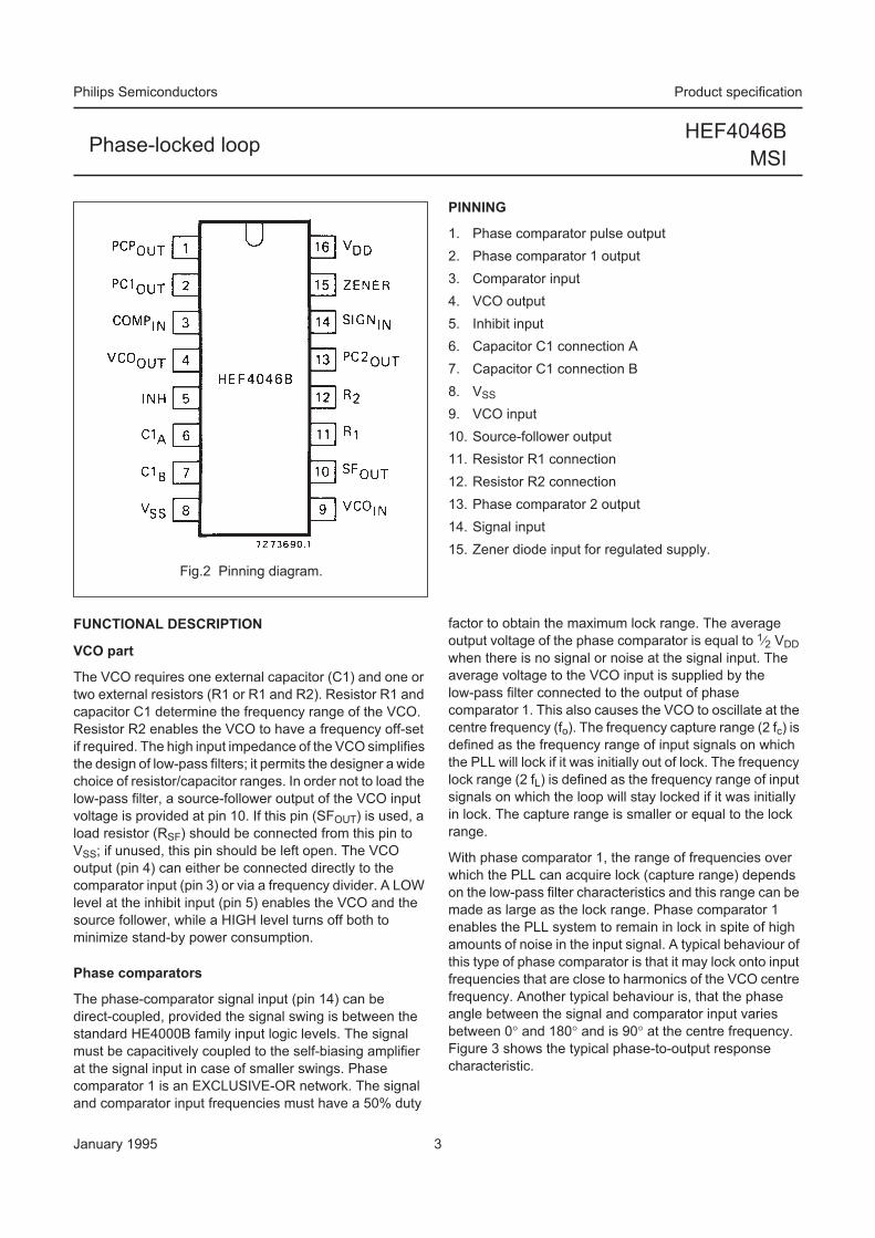
January 1995 3
Philips Semiconductors Product specification
Phase-locked loopHEF4046B
MSI
Fig.2 Pinning diagram.
PINNING
1. Phase comparator pulse output
2. Phase comparator 1 output
3. Comparator input
4. VCO output
5. Inhibit input
6. Capacitor C1 connection A
7. Capacitor C1 connection B
8. VSS
9. VCO input
10. Source-follower output
11. Resistor R1 connection
12. Resistor R2 connection
13. Phase comparator 2 output
14. Signal input
15. Zener diode input for regulated supply.
FUNCTIONAL DESCRIPTION
VCO part
The VCO requires one external capacitor (C1) and one or
two external resistors (R1 or R1 and R2). Resistor R1 and
capacitor C1 determine the frequency range of the VCO.
Resistor R2 enables the VCO to have a frequency off-set
if required. The high input impedance of the VCO simplifies
the design of low-pass filters; it permits the designer a wide
choice of resistor/capacitor ranges. In order not to load the
low-pass filter, a source-follower output of the VCO input
voltage is provided at pin 10. If this pin (SFOUT) is used, a
load resistor (RSF) should be connected from this pin to
VSS; if unused, this pin should be left open. The VCO
output (pin 4) can either be connected directly to the
comparator input (pin 3) or via a frequency divider. A LOW
level at the inhibit input (pin 5) enables the VCO and the
source follower, while a HIGH level turns off both to
minimize stand-by power consumption.
Phase comparators
The phase-comparator signal input (pin 14) can be
direct-coupled, provided the signal swing is between the
standard HE4000B family input logic levels. The signal
must be capacitively coupled to the self-biasing amplifier
at the signal input in case of smaller swings. Phase
comparator 1 is an EXCLUSIVE-OR network. The signal
and comparator input frequencies must have a 50% duty
factor to obtain the maximum lock range. The average
output voltage of the phase comparator is equal to 1⁄2 VDD
when there is no signal or noise at the signal input. The
average voltage to the VCO input is supplied by the
low-pass filter connected to the output of phase
comparator 1. This also causes the VCO to oscillate at the
centre frequency (fo). The frequency capture range (2 fc) is
defined as the frequency range of input signals on which
the PLL will lock if it was initially out of lock. The frequency
lock range (2 fL) is defined as the frequency range of input
signals on which the loop will stay locked if it was initially
in lock. The capture range is smaller or equal to the lock
range.
With phase comparator 1, the range of frequencies over
which the PLL can acquire lock (capture range) depends
on the low-pass filter characteristics and this range can be
made as large as the lock range. Phase comparator 1
enables the PLL system to remain in lock in spite of high
amounts of noise in the input signal. A typical behaviour of
this type of phase comparator is that it may lock onto input
frequencies that are close to harmonics of the VCO centre
frequency. Another typical behaviour is, that the phase
angle between the signal and comparator input varies
between 0° and 180° and is 90° at the centre frequency.
Figure 3 shows the typical phase-to-output response
characteristic.
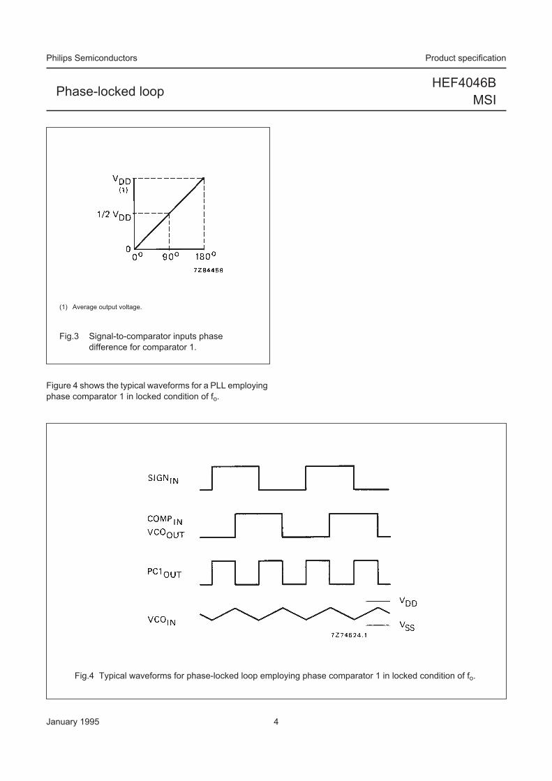
January 1995 4
Philips Semiconductors Product specification
Phase-locked loopHEF4046B
MSI
Figure 4 shows the typical waveforms for a PLL employing
phase comparator 1 in locked condition of fo.
Fig.3 Signal-to-comparator inputs phase
difference for comparator 1.
(1) Average output voltage.
Fig.4 Typical waveforms for phase-locked loop employing phase comparator 1 in locked condition of fo.

January 1995 5
Philips Semiconductors Product specification
Phase-locked loopHEF4046B
MSI
Phase comparator 2 is an edge-controlled digital memory
network. It consists of four flip-flops, control gating and a
3-state output circuit comprising p and n-type drivers
having a common output node. When the p-type or n-type
drivers are ON, they pull the output up to VDD or down to
VSS respectively. This type of phase comparator only acts
on the positive-going edges of the signals at SIGNIN and
COMPIN. Therefore, the duty factors of these signals are
not of importance.
If the signal input frequency is higher than the comparator
input frequency, the p-type output driver is maintained ON
most of the time, and both the n and p-type drivers are
OFF (3-state) the remainder of the time. If the signal input
frequency is lower than the comparator input frequency,
the n-type output driver is maintained ON most of the time,
and both the n and p-type drivers are OFF the remainder
of the time. If the signal input and comparator input
frequencies are equal, but the signal input lags the
comparator input in phase, the n-type output driver is
maintained ON for a time corresponding to the phase
difference. If the comparator input lags the signal input in
phase, the p-type output driver is maintained ON for a time
corresponding to the phase difference. Subsequently, the
voltage at the capacitor of the low-pass filter connected to
this phase comparator is adjusted until the signal and
comparator inputs are equal in both phase and frequency.
At this stable point, both p and n-type drivers remain OFF
and thus the phase comparator output becomes an open
circuit and keeps the voltage at the capacitor of the
low-pass filter constant.
Moreover, the signal at the phase comparator pulse output
(PCPOUT) is a HIGH level which can be used for indicating
a locked condition. Thus, for phase comparator 2 no phase
difference exists between the signal and comparator
inputs over the full VCO frequency range. Moreover, the
power dissipation due to the low-pass filter is reduced
when this type of phase comparator is used because both
p and n-type output drivers are OFF for most of the signal
input cycle. It should be noted that the PLL lock range for
this type of phase comparator is equal to the capture
range, independent of the low-pass filter. With no signal
present at the signal input, the VCO is adjusted to its
lowest frequency for phase comparator 2 . Figure 5 shows
typical waveforms for a PLL employing this type of phase
comparator in locked condition.
Fig.5 Typical waveforms for phase-locked loop employing phase comparator 2 in locked condition.
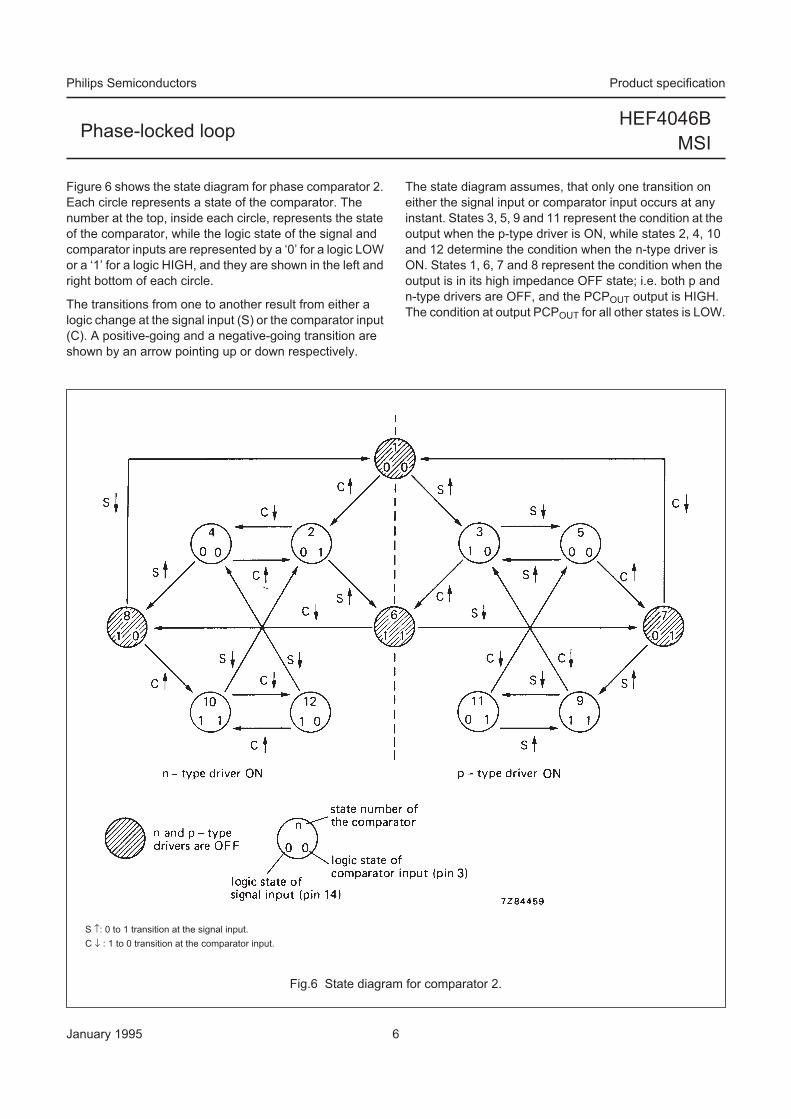
January 1995 6
Philips Semiconductors Product specification
Phase-locked loopHEF4046B
MSI
Figure 6 shows the state diagram for phase comparator 2.
Each circle represents a state of the comparator. The
number at the top, inside each circle, represents the state
of the comparator, while the logic state of the signal and
comparator inputs are represented by a ‘0’ for a logic LOW
or a ‘1’ for a logic HIGH, and they are shown in the left and
right bottom of each circle.
The transitions from one to another result from either a
logic change at the signal input (S) or the comparator input
(C). A positive-going and a negative-going transition are
shown by an arrow pointing up or down respectively.
The state diagram assumes, that only one transition on
either the signal input or comparator input occurs at any
instant. States 3, 5, 9 and 11 represent the condition at the
output when the p-type driver is ON, while states 2, 4, 10
and 12 determine the condition when the n-type driver is
ON. States 1, 6, 7 and 8 represent the condition when the
output is in its high impedance OFF state; i.e. both p and
n-type drivers are OFF, and the PCPOUT output is HIGH.
The condition at output PCPOUT for all other states is LOW.
Fig.6 State diagram for comparator 2.
S ↑: 0 to 1 transition at the signal input.
C ↓ : 1 to 0 transition at the comparator input.
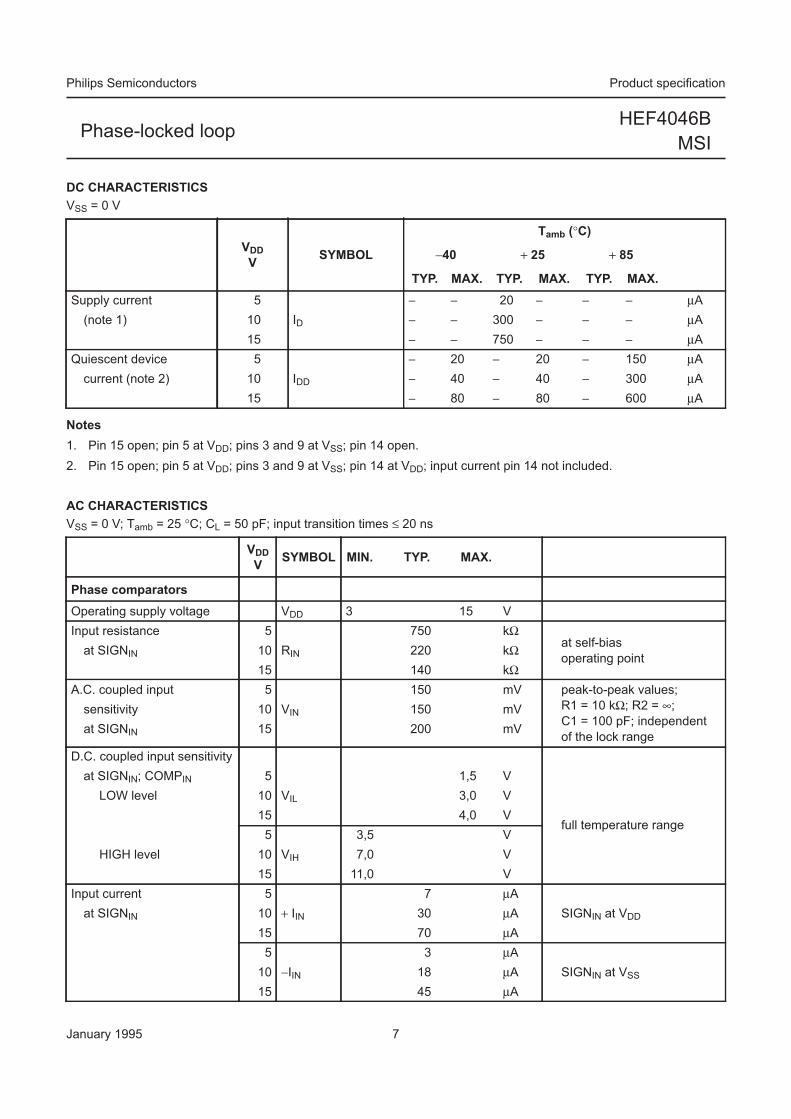
January 1995 7
Philips Semiconductors Product specification
Phase-locked loopHEF4046B
MSI
DC CHARACTERISTICS
VSS = 0 V
Notes
1. Pin 15 open; pin 5 at VDD; pins 3 and 9 at VSS; pin 14 open.
2. Pin 15 open; pin 5 at VDD; pins 3 and 9 at VSS; pin 14 at VDD; input current pin 14 not included.
AC CHARACTERISTICS
VSS = 0 V; Tamb = 25 °C; CL = 50 pF; input transition times ≤ 20 ns
VDD
VSYMBOL
Tamb (°C)
−40 + 25 + 85
TYP. MAX. TYP. MAX. TYP. MAX.
Supply current 5 − − 20 − − − µA
(note 1) 10 ID − − 300 − − − µA
15 − − 750 − − − µA
Quiescent device 5 − 20 − 20 − 150 µA
current (note 2) 10 IDD − 40 − 40 − 300 µA
15 − 80 − 80 − 600 µA
VDD
VSYMBOL MIN. TYP. MAX.
Phase comparators
Operating supply voltage VDD 3 15 V
Input resistance 5 750 kΩat self-bias
operating pointat SIGNIN 10 RIN 220 kΩ
15 140 kΩ
A.C. coupled input 5 150 mV peak-to-peak values;
R1 = 10 kΩ; R2 = ∞;
C1 = 100 pF; independent
of the lock range
sensitivity 10 VIN 150 mV
at SIGNIN 15 200 mV
D.C. coupled input sensitivity
at SIGNIN; COMPIN 5 1,5 V
full temperature range
LOW level 10 VIL 3,0 V
15 4,0 V
5 3,5 V
HIGH level 10 VIH 7,0 V
15 11,0 V
Input current 5 7 µA
SIGNIN at VDDat SIGNIN 10 + IIN 30 µA
15 70 µA
5 3 µA
SIGNIN at VSS10 −IIN 18 µA
15 45 µA
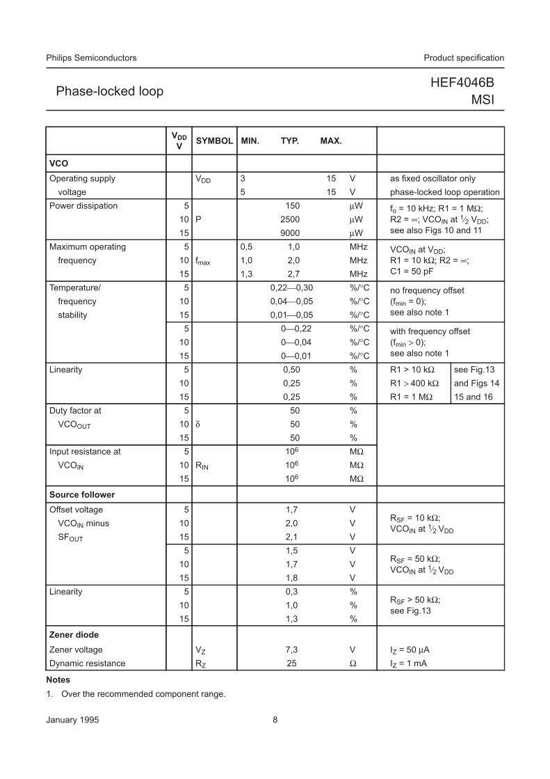
January 1995 8
Philips Semiconductors Product specification
Phase-locked loopHEF4046B
MSI
Notes
1. Over the recommended component range.
VCO
Operating supply VDD 3 15 V as fixed oscillator only
voltage 5 15 V phase-locked loop operation
Power dissipation 5 150 µW fo = 10 kHz; R1 = 1 MΩ;
R2 = ∞; VCOIN at 1⁄2 VDD;
see also Figs 10 and 11
10 P 2500 µW
15 9000 µW
Maximum operating 5 0,5 1,0 MHz VCOIN at VDD;
R1 = 10 kΩ; R2 = ∞;
C1 = 50 pF
frequency 10 fmax 1,0 2,0 MHz
15 1,3 2,7 MHz
Temperature/ 5 0,220,30 %/°C no frequency offset
(fmin = 0);
see also note 1
frequency 10 0,040,05 %/°C
stability 15 0,010,05 %/°C
5 00,22 %/°C with frequency offset
(fmin > 0);
see also note 1
10 00,04 %/°C
15 00,01 %/°C
Linearity 5 0,50 % R1 > 10 kΩ see Fig.13
10 0,25 % R1 > 400 kΩ and Figs 14
15 0,25 % R1 = 1 MΩ 15 and 16
Duty factor at 5 50 %
VCOOUT 10 δ 50 %
15 50 %
Input resistance at 5 106 MΩ
VCOIN 10 RIN 106 MΩ
15 106 MΩ
Source follower
Offset voltage 5 1,7 VRSF = 10 kΩ;
VCOIN at 1⁄2 VDDVCOIN minus 10 2,0 V
SFOUT 15 2,1 V
5 1,5 VRSF = 50 kΩ;
VCOIN at 1⁄2 VDD10 1,7 V
15 1,8 V
Linearity 5 0,3 %RSF > 50 kΩ;
see Fig.1310 1,0 %
15 1,3 %
Zener diode
Zener voltage VZ 7,3 V IZ = 50 µA
Dynamic resistance RZ 25 Ω IZ = 1 mA
VDD
VSYMBOL MIN. TYP. MAX.

January 1995 9
Philips Semiconductors Product specification
Phase-locked loopHEF4046B
MSI
DESIGN INFORMATION
VCO component selection
Recommended range for R1 and R2: 10 kΩ to 1 MΩ; for C1: 50 pF to any practical value.
1. VCO without frequency offset (R2 = ∞).
a) Given fo: use fo with Fig.7 to determine R1 and C1.
b) Given fmax: calculate fo from fo = 1⁄2 fmax; use fo with Fig.7 to determine R1 and C1.
2. VCO with frequency offset.
a) Given fo and fL : calculate fmin from the equation fmin = fo − fL; use fmin with Fig.8 to determine R2 and C1; calculate
b) Given fmin and fmax: use fmin with Fig.8 to determine R2 and C1; calculate
with Fig.9 to determine R2/R1 to obtain R1.
CHARACTERISTIC USING PHASE COMPARATOR 1 USING PHASE COMPARATOR 2
No signal on SIGNIN VCO in PLL system adjusts
to centre frequency (fo)
VCO in PLL system adjusts to min.
frequency (fmin)
Phase angle between
SIGNIN and COMPIN
90° at centre frequency (fo),
approaching 0° and 180° at
ends of lock range (2 fL)
always 0° in lock
(positive-going edges)
Locks on harmonics of
centre frequency
yes no
Signal input noise
rejection
high low
Lock frequency
range (2 fL)
the frequency range of the input signal on which the loop will stay locked if it was
initially in lock; 2 fL = full VCO frequency range = fmax − fmin
Capture frequency
range (2 fC)
the frequency range of the input signal on which the loop will lock if it was initially
out of lock
depends on low-pass
filter characteristics; fC < fL
fC = fL
Centre frequency (fo) the frequency of the VCO when VCOIN at 1⁄2VDD
fmax
fmin
----------- from the equationfmax
fmin
-----------
fo fL+
fo fL–--------------- ; use
fmax
fmin
----------- with Fig. 9 to determine the ratio R2/R1 to obtain R1.=
fmax
fmin
----------- ; usefmax
fmin
-----------
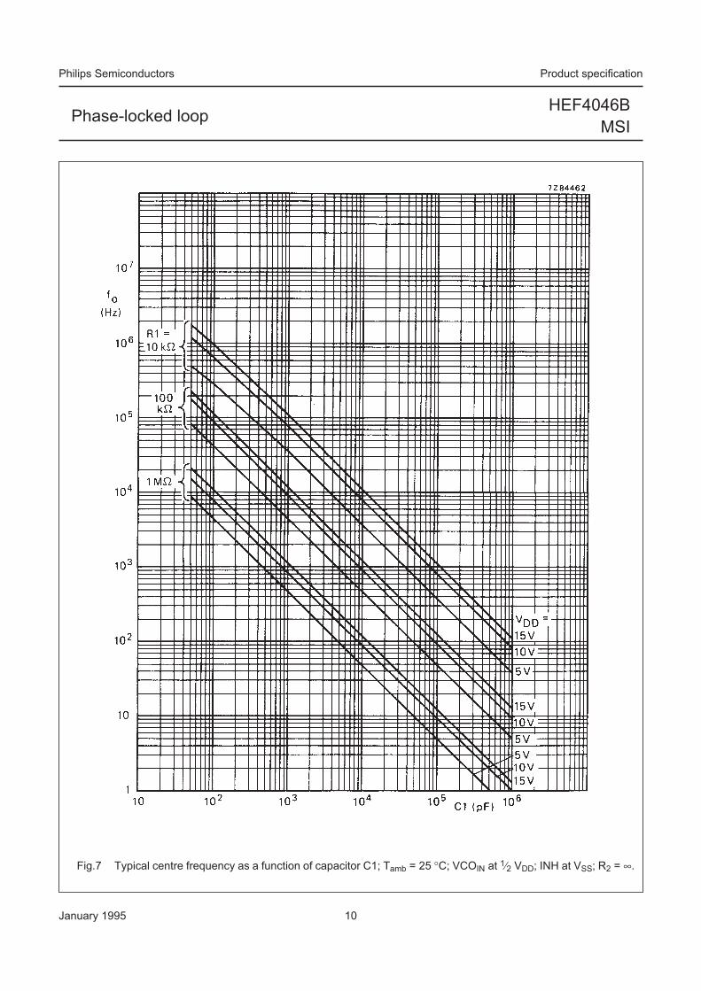
January 1995 10
Philips Semiconductors Product specification
Phase-locked loopHEF4046B
MSI
Fig.7 Typical centre frequency as a function of capacitor C1; Tamb = 25 °C; VCOIN at 1⁄2 VDD; INH at VSS; R2 = ∞.
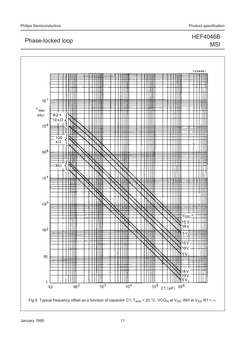
January 1995 11
Philips Semiconductors Product specification
Phase-locked loopHEF4046B
MSI
Fig.8 Typical frequency offset as a function of capacitor C1; Tamb = 25 °C; VCOIN at VSS; INH at VSS; R1 = ∞.
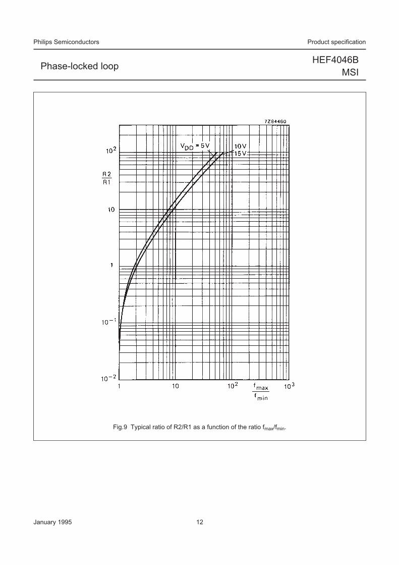
January 1995 12
Philips Semiconductors Product specification
Phase-locked loopHEF4046B
MSI
Fig.9 Typical ratio of R2/R1 as a function of the ratio fmax/fmin.
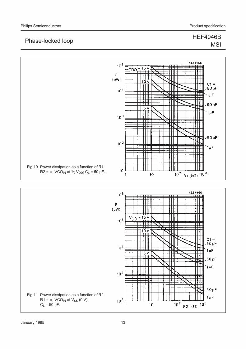
January 1995 13
Philips Semiconductors Product specification
Phase-locked loopHEF4046B
MSI
Fig.10 Power dissipation as a function of R1;
R2 = ∞; VCOIN at 1⁄2 VDD; CL = 50 pF.
Fig.11 Power dissipation as a function of R2;
R1 = ∞; VCOIN at VSS (0 V);
CL = 50 pF.
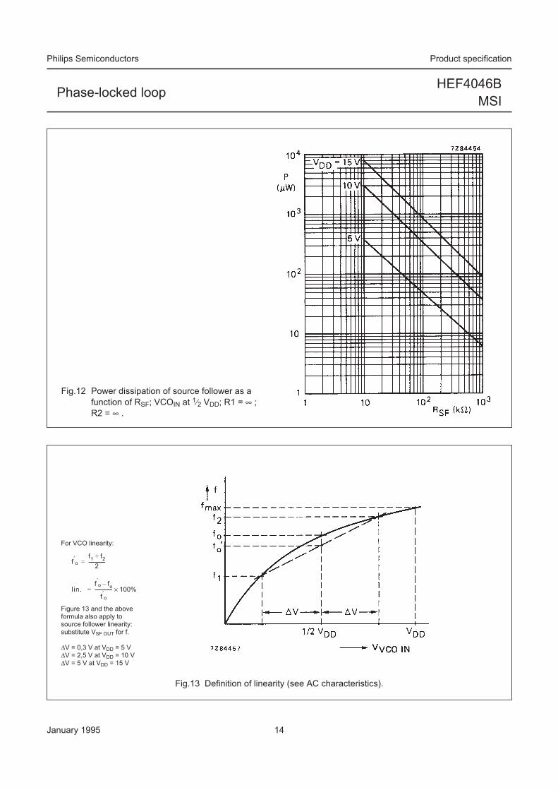
January 1995 14
Philips Semiconductors Product specification
Phase-locked loopHEF4046B
MSI
Fig.12 Power dissipation of source follower as a
function of RSF; VCOIN at 1⁄2 VDD; R1 = ∞ ;
R2 = ∞ .
Fig.13 Definition of linearity (see AC characteristics).
For VCO linearity:
Figure 13 and the aboveformula also apply tosource follower linearity:substitute VSF OUT for f.
∆V = 0,3 V at VDD = 5 V∆V = 2,5 V at VDD = 10 V∆V = 5 V at VDD = 15 V
f′o
f1 f2+
2---------------=
l in.f′o fo–
f′o
---------------- 100%×=
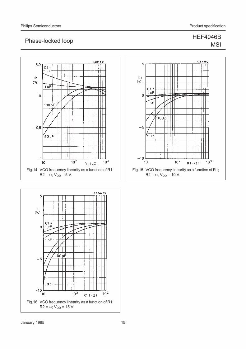
January 1995 15
Philips Semiconductors Product specification
Phase-locked loopHEF4046B
MSI
Fig.14 VCO frequency linearity as a function of R1;
R2 = ∞; VDD = 5 V.
Fig.15 VCO frequency linearity as a function of R1;
R2 = ∞; VDD = 10 V.
Fig.16 VCO frequency linearity as a function of R1;
R2 = ∞; VDD = 15 V.

This datasheet has been download from:
www.datasheetcatalog.com
Datasheets for electronics components.