SchedulingScheduling
Levels of schedulingLevels of scheduling
AlgorithmsAlgorithms

C.Brandolese - 2 -
IntroductionIntroduction
Scheduling
Decides which process to execute at a certain
moment
Is implemented by a specific component
The scheduler
Schedulers differ according to their goal
Maximize throughput
Minimize latency
Maximize processor usage
Avoid starvation
Complete a process within a predefined time
Real time scheduling

C.Brandolese - 3 -
Levels ofLevels of schedulingscheduling
Complex OS may have different schedulers
Long-term scheduler
Admits processes
New → Ready, New → Ready-Suspend
Determines the number of processes in a system
Medium-term scheduler
Determines which processes may compete for CPU
Ready ↔ Ready-Suspend, Blocked ↔ Blocked-Suspend
Reacts to medium-term processor load fluctuations
Short-term scheduler
Assigns processes to the processor
Ready ↔ Running
Manages priorities
C.Brandolese - 4 -
Levels of schedulingLevels of scheduling
long-term
medium-term
short-term
New
Exit
Admit
Admit
Release
long-term
medium-term
short-term

C.Brandolese - 5 -
Levels of schedulingLevels of scheduling
batchjobs
interactive users
DispatchCPU
Release
Ready queue
Event waitEvent occurs
Timeout
Ready suspend queue
Blocked suspend queue
Blocked queue
long-term
short-term
medium-term

C.Brandolese - 6 -
DispatcherDispatcher
Short term scheduler
Called dispatcher
Executed very frequently
Invoked on specific events
I/O and clock interrupt
System call
Signal (software interrupt)
Scheduling criteria
User-oriented
Minimizes the response time
System-oriented
Efficient usage of the processor

C.Brandolese - 7 -
PreemptionPreemption
Scheduling policies can be
Preemptive
Nonpreemptive
Preemptive scheduling
Processes can be interrupted
Tend to rdeuce the response time
Useful in highly interactive systems
Nonpreemptive scheduling
Processes run to completion
A process can block other processes for an
undefinitely long time
C.Brandolese - 8 -
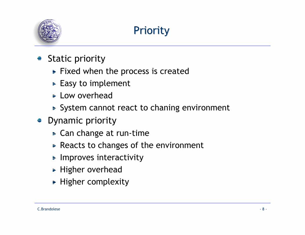
PriorityPriority
Static priority
Fixed when the process is created
Easy to implement
Low overhead
System cannot react to chaning environment
Dynamic priority
Can change at run-time
Reacts to changes of the environment
Improves interactivity
Higher overhead
Higher complexity
C.Brandolese - 9 -
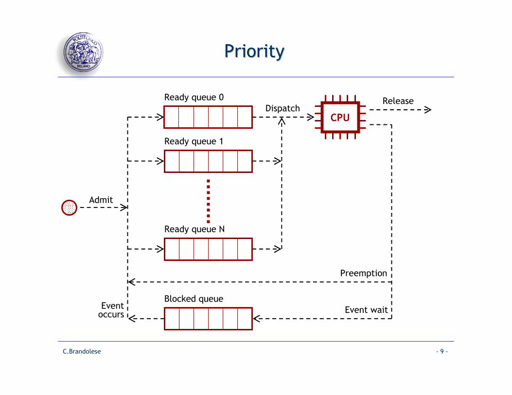
PriorityPriority
CPU
Ready queue 0
Ready queue 1
Admit
Ready queue N
Blocked queue
DispatchRelease
Event wait
Preemption
Eventoccurs
C.Brandolese - 10 -
FIFO or FCFSFIFO or FCFS
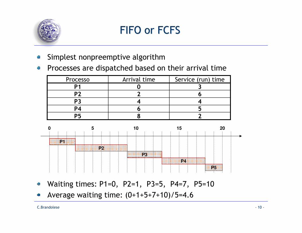
Simplest nonpreemptive algorithm
Processes are dispatched based on their arrival time
Waiting times: P1=0, P2=1, P3=5, P4=7, P5=10
Average waiting time: (0+1+5+7+10)/5=4.6
28P5
56P4
44P3
62P2
30P1
Service (run) timeArrival timeProcesso
P1
0 5 10 15 20
P2
P3
P4
P5

C.Brandolese - 11 -
FIFO or FCFSFIFO or FCFS
Algorithm
A new process is inserted in the ready queue
When a process terminates, the oldest process in the
queue is dispatched
Limitations
A short process may be delayed by a long one
Favors CPU-bound processes
I/O-bound processes must wait for CPU/bound
processes to complete

C.Brandolese - 12 -
FIFO or FCFSFIFO or FCFS
Processi
Case 1: Arrival order is P1, P2, P3
Waiting times: P1=0, P2=24, P3=27
Average waiting time: (0+24+27)/3=17
30P3
30P2
240P1
Service (run) timeArrival timeProcesso
P1
0
P2
P3
24 27 30

C.Brandolese - 13 -
FIFO o FCFS FIFO o FCFS –– FirstFirst--Come, FirstCome, First--
Serve Serve
30P3
30P2
240P1
Service (run) timeArrival timeProcesso
P1
0
P2
P3
3 6 30
Processi
Case 1: Arrival order is P2, P3, P1
Waiting times: P1=6, P2=0, P3=3
Average waiting time: (6+0+3)/3=3

C.Brandolese - 14 -
RR RR –– Round RobinRound Robin
Preemptive algorithms
Processes are served FIFO
Process can run for a fixed amount of time
Timeslice
If a process does not terminate within its timeslice
The system
Preempts it
Re-queues the process at the end of the queue
The first process in queue is dispatched

C.Brandolese - 15 -
RR RR –– Round RobinRound Robin
Processes
Timeslice is 3 “units”
Waiting times: P1=0+3+3, P2=1, P3=4+3, P4=3+2
Tempo medio di attesa: (6+1+7+5)/4=4.75
510P4
55P3
32P2
70P1
Service (run) timeArrival timeProcesso
P1
P2
P3
P4
0 5 10 15 20
P1 P1
P3
P4

C.Brandolese - 16 -
SRR SRR –– Selfish Round RobinSelfish Round Robin
Variation of RR
Each process has an initial priority
Process get old and increase their priority
Often implemented with an additional queue
A process enters the queue of new process
It gets old, and when its priority equals that of ready
processes is dispatched
CPU
Ready queue
New processes queue
Admit
DispatchRelease
When process old enough andPriority equat to that in the ready queue

C.Brandolese - 17 -
RR/SRR and TimesliceRR/SRR and Timeslice
What is the optimal duration of the timeslice?
Short or long?
Fixed or variable?
The same for all processes?
Long timeslice
Probably sufficient to run processes to completion
RR algorithm becomes equivalent to FIFO
Short timeslice
Context switch overhead becomes significant
Typical timeslices
Desktop computing: 20ms – 100ms
Real-time computing: 1ms
C.Brandolese - 18 -
SJF SJF –– Shortest Job FirstShortest Job First
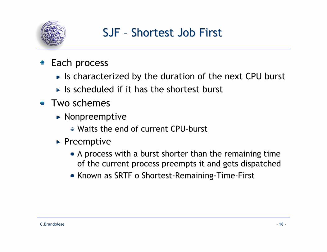
Each process
Is characterized by the duration of the next CPU burst
Is scheduled if it has the shortest burst
Two schemes
Nonpreemptive
Waits the end of current CPU-burst
Preemptive
A process with a burst shorter than the remaining time
of the current process preempts it and gets dispatched
Known as SRTF o Shortest-Remaining-Time-First

C.Brandolese - 19 -
SJF SJF –– Shortest Job FirstShortest Job First
Requires estimating the duration of the next burst
Adaptive approach
Estimations are performed for each processes
Computationally light
Exponntial average estimation is often used
τn+1 = αtn + (1- α)τn
Where
tn Actual burst duration at time n (current)
τn+1 Estimated burst duration at time n+1
α Coefficient between 0 and 1

C.Brandolese - 20 -
SJF SJF –– Shortest Job FirstShortest Job First
The behaviour strongly dependes on α
α = 0
τn+1 = τnThe history of the system is unimportant
α = 1
τn+1 = tnOnly the last burst considered
0 ≤ α ≤ 1
The importance of older estimates (τn) tend to
exponentially decrease as (1-α)n

C.Brandolese - 21 -
SJF SJF –– Shortest Job FirstShortest Job First
Processi
Nonpreemptive
Waiting times: P1=0, P2=6, P3=3, P4=7
Average waiting time: (0+6+3+7)/4=4
45P4
14P3
42P2
70P1
Burst timeArrival timeProcesso
P1
0 5 10 15 20
P3
P2
P4
C.Brandolese - 22 -
SJF SJF –– Shortest Job FirstShortest Job First
Processi
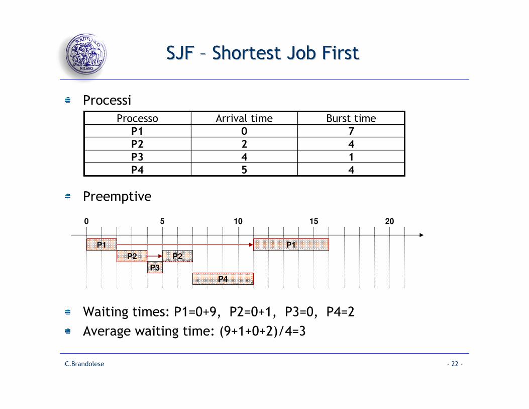
Preemptive
Waiting times: P1=0+9, P2=0+1, P3=0, P4=2
Average waiting time: (9+1+0+2)/4=3
45P4
14P3
42P2
70P1
Burst timeArrival timeProcesso
P1
0 5 10 15 20
P2
P4
P1
P3
P2

C.Brandolese - 23 -
SPN SPN –– Shortest Process NextShortest Process Next
Nonpreemptive scheme
The ready process with shortes estimated run time is selected
Waiting times: P1=0, P2=1, P3=7, P4=9, P5=1
Average waiting time: (0+1+7+9+1)/5=3.6
28P5
56P4
44P3
62P2
30P1
Service (run) timeArrival timeProcesso
P1
0 5 10 15 20
P2
P3
P4
P5

C.Brandolese - 24 -
SPN SPN –– Shortest Process NextShortest Process Next
Advantages
Shorter process are served rapidly
Problems
Long process can be daleyed for long time
Potential starvation
Reduces process completion predictability
Strongly depends from the accuracy of the estimated
completion times
Wrong estimates might require terminating a process

C.Brandolese - 25 -
HRRN HRRN –– Highest Response Ratio NextHighest Response Ratio Next
Overcomes the limitations of SJF/SPN algorithms
Nonpreeptive algorithm
Re-calcultaes the priority of each process
Selects the process with highest priority
Priority is evaluated as:
Considerations
Short processes are favored since execution time
appears at the denominator
Process waiting since long time are favored since
waiting time is on the numerator
(Tattesa + Texec)
Texec

C.Brandolese - 26 -
SRT SRT –– Shortest Remaining TimeShortest Remaining Time
Preemptive version of SPN
Requires remaining execution time estimation
Waiting times: P1=0, P2=1+6, P3=0, P4=9, P5=0
Average waiting time: (0+7+0+9+0)/5=3.2
28P5
56P4
44P3
62P2
30P1
Service (run) timeArrival timeProcesso
P1
0 5 10 15 20
P2
P3
P4
P5
P2
C.Brandolese - 27 -
FSS FSS –– Fair Share SchedulingFair Share Scheduling
Processi in a system sistema
Are often related to each other
Can be grouped according to some criterion
Same user or group
Same application
…
Groups can have different importance
FSS
Prevents that certain groups consume all resources
Distributes resources over groups
According to some criterion

C.Brandolese - 28 -
FSS FSS –– Fair Share SchedulingFair Share Scheduling
Traditional approach
Single scheduler
100% resource equally
shared by all processes
FSS
Two scheduing levels
Fair share
Processes
Resource are assigned
to grops according to
a predefined scheme