Scaling up Bayesian Inference
David Dunson
Departments of Statistical Science, Mathematics & ECE, Duke University
May 1, 2017

Outline
Motivation & background
EP-MCMC
aMCMC
Discussion
Motivation & background 2

Complex & high-dimensional data
j Interest in developing new methods for analyzing & interpretingcomplex, high-dimensional data
j Arise routinely in broad fields of sciences, engineering & evenarts & humanities
j Despite huge interest in big data, there are vast gaps that havefundamentally limited progress in many fields
Motivation & background 2

‘Typical’ approaches to big data
j There is an increasingly immense literature focused on big data
j Most of the focus has been on optimization-style methods
j Rapidly obtaining a point estimate even when sample size n &overall ‘size’ of data is immense
j Bandwagons: many people work on quite similar problems,while critical open problems remain untouched
Motivation & background 3

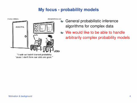
My focus - probability models
j General probabilistic inferencealgorithms for complex data
j We would like to be able to handlearbitrarily complex probability models
j Algorithms scalable to huge data -potentially using many computers
j Accurate uncertainty quantification (UQ) is a critical issue
j Robustness of inferences also crucial
j Particular emphasis on scientific applications - limited labeleddata
Motivation & background 4

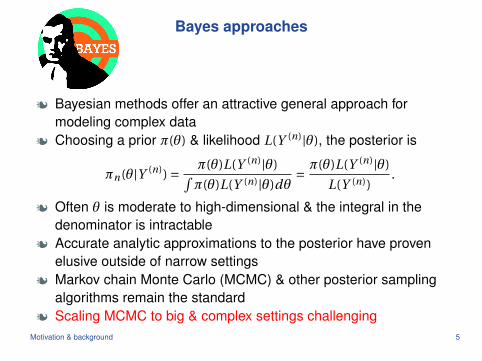
Bayes approaches
j Bayesian methods offer an attractive general approach formodeling complex data
j Choosing a prior π(θ) & likelihood L(Y (n)|θ), the posterior is
πn(θ|Y (n)) = π(θ)L(Y (n)|θ)∫π(θ)L(Y (n)|θ)dθ
= π(θ)L(Y (n)|θ)
L(Y (n)).
j Often θ is moderate to high-dimensional & the integral in thedenominator is intractable
j Accurate analytic approximations to the posterior have provenelusive outside of narrow settings
j Markov chain Monte Carlo (MCMC) & other posterior samplingalgorithms remain the standard
j Scaling MCMC to big & complex settings challenging
Motivation & background 5
Bayes approaches
j Bayesian methods offer an attractive general approach formodeling complex data
j Choosing a prior π(θ) & likelihood L(Y (n)|θ), the posterior is
πn(θ|Y (n)) = π(θ)L(Y (n)|θ)∫π(θ)L(Y (n)|θ)dθ
= π(θ)L(Y (n)|θ)
L(Y (n)).
j Often θ is moderate to high-dimensional & the integral in thedenominator is intractable
j Accurate analytic approximations to the posterior have provenelusive outside of narrow settings
j Markov chain Monte Carlo (MCMC) & other posterior samplingalgorithms remain the standard
j Scaling MCMC to big & complex settings challengingMotivation & background 5

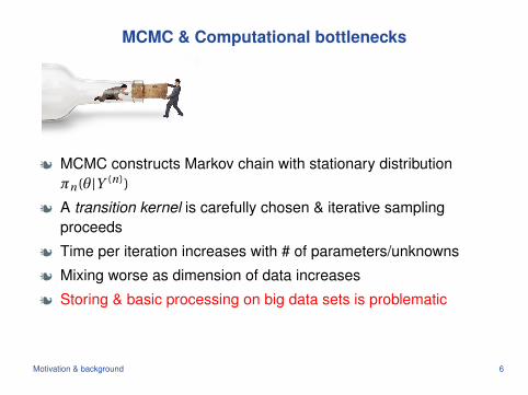
MCMC & Computational bottlenecks
j MCMC constructs Markov chain with stationary distributionπn(θ|Y (n))
j A transition kernel is carefully chosen & iterative samplingproceeds
j Time per iteration increases with # of parameters/unknowns
j Mixing worse as dimension of data increases
j Storing & basic processing on big data sets is problematic
j Usually multiple likelihood and/or gradient evaluations at eachiteration
Motivation & background 6

Solutions
j Embarrassingly parallel (EP) MCMC: run MCMC in parallel fordifferent subsets of data & combine.
j Approximate MCMC: Approximate expensive to evaluatetransition kernels.
j Hybrid algorithms: run MCMC for a subset of the parameters& use a fast estimate for the others.
j Designer MCMC: define clever kernels that solve mixingproblems in high dimensions
j I’ll focus on EP-MCMC & aMCMC in remainder
Motivation & background 7

Outline
Motivation & background
EP-MCMC
aMCMC
Discussion
EP-MCMC 8

Embarrassingly parallel MCMC
j Divide large sample size n data set into many smaller data setsstored on different machines
j Draw posterior samples for each subset posterior in parallelj ‘Magically’ combine the results quickly & simply
EP-MCMC 8

Embarrassingly parallel MCMC
j Divide large sample size n data set into many smaller data setsstored on different machines
j Draw posterior samples for each subset posterior in parallel
j ‘Magically’ combine the results quickly & simply
EP-MCMC 8

Embarrassingly parallel MCMC
j Divide large sample size n data set into many smaller data setsstored on different machines
j Draw posterior samples for each subset posterior in parallelj ‘Magically’ combine the results quickly & simply
EP-MCMC 8

Toy Example: Logistic Regression
200
400
600 800
1000
1200
200
400
600 800
1000
1200
200
400
600
800
100
0
1200
1600
200
400
600
800
100
0
1600
200
400
600
800
100
0 120
0
200
400
600 800
1000 1200 200
400
600
800
1000 120
0
200
400 600
800 1000
1600
200
400
600
800
100
0
1200
1800
200
400
600
800
100
0
1200 160
0
200
400
600
800
1000
120
0
200
400
600
800
1000
120
0
1600
200
400
600 800
1000
120
0
1600
200
400
600
800
1000
1200
200
400
600
800
1000 120
0
1400
200
400
600
800
100
0
140
0
1600
200
400
600
800
100
0
1600
200
400
600
800
1000 120
0
200
400
600
800 1000
1600
200
400 600
800
1000 120
0
1600
200
400
600
800
1000
1600
200
400
600
800
1000
1200
200
400
600
800 100
0
1200
160
0
200
400 600
800
100
0 1200 1600
200
400
600 800
1000
1400
200
400
600
800
1000 120
0
1600
200
400 600
800
1000 120
0
1600
200
400
600 800
1000 1200
200
400 600
800
1000
1200
1400
200
400
600
800
1000
200
400
600
800
100
0
1400
200
400
600
800
100
0
120
0 1800
200
400
600
800 100
0
120
0 1
400
200
400
600 800
1000
1200
200
400
600
800 1000
120
0
1600
200
400
600
800
1000
1200
140
0
200
400
600
800
1000
1200
200
400
600
800
1000
120
0 1600
200
400
600
800 1000 1400
200
400
600
800
1000 120
0
1800
200
400
600
800
1000
120
0
1800
−1.15 −1.10 −1.05 −1.00 −0.95 −0.90 −0.850.85
0.90
0.95
1.00
1.05
1.10
1.15
200
400
600
800
1000 120
0
500
1000
1500
2000
MCMCSubset PosteriorWASP
β1
β 2
pr(yi = 1|xi 1, . . . , xi p ,θ) =exp
(∑pj=1 xi jβ j
)1+exp
(∑pj=1 xi jβ j
) .
j Subset posteriors: ‘noisy’ approximations of full data posterior.
j ‘Averaging’ of subset posteriors reduces this ‘noise’ & leads toan accurate posterior approximation.
EP-MCMC 9

Toy Example: Logistic Regression
200
400
600 800
1000
1200
200
400
600 800
1000
1200
200
400
600
800
100
0
1200
1600
200
400
600
800
100
0
1600
200
400
600
800
100
0 120
0
200
400
600 800
1000 1200 200
400
600
800
1000 120
0
200
400 600
800 1000
1600
200
400
600
800
100
0
1200
1800
200
400
600
800
100
0
1200 160
0
200
400
600
800
1000
120
0
200
400
600
800
1000
120
0
1600
200
400
600 800
1000
120
0
1600
200
400
600
800
1000
1200
200
400
600
800
1000 120
0
1400
200
400
600
800
100
0
140
0
1600
200
400
600
800
100
0
1600
200
400
600
800
1000 120
0
200
400
600
800 1000
1600
200
400 600
800
1000 120
0
1600
200
400
600
800
1000
1600
200
400
600
800
1000
1200
200
400
600
800 100
0
1200
160
0
200
400 600
800
100
0 1200 1600
200
400
600 800
1000
1400
200
400
600
800
1000 120
0
1600
200
400 600
800
1000 120
0
1600
200
400
600 800
1000 1200
200
400 600
800
1000
1200
1400
200
400
600
800
1000
200
400
600
800
100
0
1400
200
400
600
800
100
0
120
0 1800
200
400
600
800 100
0
120
0 1
400
200
400
600 800
1000
1200
200
400
600
800 1000
120
0
1600
200
400
600
800
1000
1200
140
0
200
400
600
800
1000
1200
200
400
600
800
1000
120
0 1600
200
400
600
800 1000 1400
200
400
600
800
1000 120
0
1800
200
400
600
800
1000
120
0
1800
−1.15 −1.10 −1.05 −1.00 −0.95 −0.90 −0.850.85
0.90
0.95
1.00
1.05
1.10
1.15
200
400
600
800
1000 120
0
500
1000
1500
2000
MCMCSubset PosteriorWASP
β1
β 2
pr(yi = 1|xi 1, . . . , xi p ,θ) =exp
(∑pj=1 xi jβ j
)1+exp
(∑pj=1 xi jβ j
) .
j Subset posteriors: ‘noisy’ approximations of full data posterior.j ‘Averaging’ of subset posteriors reduces this ‘noise’ & leads to
an accurate posterior approximation.EP-MCMC 9
Stochastic Approximation
j Full data posterior density of inid data Y (n)
πn(θ | Y (n)) =∏n
i=1 pi (yi | θ)π(θ)∫Θ
∏ni=1 pi (yi | θ)π(θ)dθ
.
j Divide full data Y (n) into k subsets of size m:Y (n) = (Y[1], . . . ,Y[ j ], . . . ,Y[k]).
j Subset posterior density for j th data subset
πγm(θ | Y[ j ]) =
∏i∈[ j ](pi (yi | θ))γπ(θ)∫
Θ
∏i∈[ j ](pi (yi | θ))γπ(θ)dθ
.
j γ=O(k) - chosen to minimize approximation error
EP-MCMC 10

Barycenter in Metric Spaces
EP-MCMC 11

Barycenter in Metric Spaces
EP-MCMC 12

WAsserstein barycenter of Subset Posteriors (WASP)
Srivastava, Li & Dunson (2015)
j 2-Wasserstein distance between µ,ν ∈P 2(Θ)
W2(µ,ν) = inf{(E[d 2(X ,Y )]
) 12 : law(X ) =µ, law(Y ) = ν
}.
j Πγm(· | Y[ j ]) for j = 1, . . . ,k are combined through WASP
Πγn(· | Y (n)) = argmin
Π∈P 2(Θ)
1
k
k∑j=1
W 22 (Π,Πγ
m(· | Y[ j ])). [Agueh & Carlier (2011)]
j Plugging in Π̂γm(· | Y[ j ]) for j = 1, . . . ,k, a linear program (LP) can
be used for fast estimation of an atomic approximation
EP-MCMC 13

LP Estimation of WASP
j Minimizing Wasserstein is solution to a discrete optimaltransport problem
j Let µ=∑J1j=1 a jδθ1 j , ν=∑J2
l=1 blδθ2l & M12 ∈ℜJ1×J2 = matrix ofsquare differences in atoms {θ1 j }, {θ2l }.
j Optimal transport polytope: T (a,b) = set of doubly stochasticmatrices w/ row sums a & column sums b
j Objective is to find T ∈T (a,b) minimizing tr(TT M12)
j For WASP, generalize to multimargin optimal transport problem- entropy smoothing has been used previously
j We can avoid such smoothing & use sparse LP solvers -neglible computation cost compared to sampling
EP-MCMC 14

WASP: Theorems
Theorem (Subset Posteriors)Under “usual” regularity conditions, there exists a constant C1
independent of subset posteriors, such that for large m,
EP [ j ]θ0
W 22
{Πγm(· | Y[ j ]),δθ0 (·)}≤C1
(log2 m
m
) 1α
j = 1, . . . ,k,
Theorem (WASP)Under “usual” regularity conditions and for large m,
W2
{Πγn(· | Y (n)),δθ0 (·)
}=OP (n)
θ0
√log2/αm
km1/α
.
EP-MCMC 15

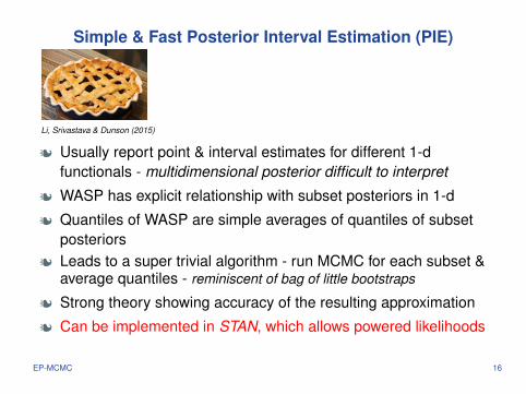
Simple & Fast Posterior Interval Estimation (PIE)
Li, Srivastava & Dunson (2015)
j Usually report point & interval estimates for different 1-dfunctionals - multidimensional posterior difficult to interpret
j WASP has explicit relationship with subset posteriors in 1-d
j Quantiles of WASP are simple averages of quantiles of subsetposteriors
j Leads to a super trivial algorithm - run MCMC for each subset &average quantiles - reminiscent of bag of little bootstraps
j Strong theory showing accuracy of the resulting approximation
j Can be implemented in STAN, which allows powered likelihoods
EP-MCMC 16

Theory on PIE/1-d WASP
j We show 1-d WASP Πn(ξ|Y (n)) is highly accurate approximationto exact posterior Πn(ξ|Y (n))
j As subset sample size m increases, W2 distance between themdecreases at faster than parametric rate op (n−1/2)
j Theorem allows k =O(nc ) and m =O(n1−c ) for any c ∈ (0,1), som can increase very slowly relative to k (recall n = mk)
j Their biases, variances, quantiles only differ in high orders ofthe total sample size
j Conditions: standard, mild conditions on likelihood + prior finite2nd moment & uniform integrabiity of subset posteriors
EP-MCMC 17
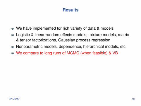
Results
j We have implemented for rich variety of data & models
j Logistic & linear random effects models, mixture models, matrix& tensor factorizations, Gaussian process regression
j Nonparametric models, dependence, hierarchical models, etc.
j We compare to long runs of MCMC (when feasible) & VB
j WASP/PIE is much faster than MCMC & highly accurate
j Carefully designed VB implementations often do very well
EP-MCMC 18

Outline
Motivation & background
EP-MCMC
aMCMC
Discussion
aMCMC 19

aMCMC Johndrow, Mattingly, Mukherjee & Dunson (2015)
j Different way to speed up MCMC - replace expensive transitionkernels with approximations
j For example, approximate a conditional distribution in Gibbssampler with a Gaussian or using a subsample of data
j Can potentially vastly speed up MCMC sampling inhigh-dimensional settings
j Original MCMC sampler converges to a stationary distributioncorresponding to the exact posterior
j Not clear what happens when we start substituting inapproximations - may diverge etc
aMCMC 19

aMCMC Overview
j aMCMC is used routinely in an essentially ad hoc manner
j Our goal: obtain theory guarantees & use these to target designof algorithms
j Define ‘exact’ MCMC algorithm, which is computationallyintractable but has good mixing
j ‘exact’ chain converges to stationary distribution correspondingto exact posterior
j Approximate kernel in exact chain with more computationallytractable alternative
aMCMC 20

Sketch of theory
j Define sε = τ1(P )/τ1(Pε) = computational speed-up, τ1(P ) =time for one step with transition kernel P
j Interest: optimizing computational time-accuracy tradeoff forestimators of Π f = ∫
Θ f (θ)Π(dθ|x)
j We provide tight, finite sample bounds on L2 error
j aMCMC estimators win for low computational budgets but haveasymptotic bias
j Often larger approximation error → larger sε & rougherapproximations are better when speed super important
aMCMC 21

Ex 1: Approximations using subsets
j Replace the full data likelihood with
Lε(x | θ) =(∏
i∈VL(xi | θ)
)N /|V |,
for randomly chosen subset V ⊂ {1, . . . ,n}.
j Applied to Pólya-Gamma data augmentation for logisticregression
j Different V at each iteration – trivial modification to Gibbsj Assumptions hold with high probability for subsets > minimal
size (wrt distribution of subsets, data & kernel).
aMCMC 22

Ex 1: Approximations using subsets
j Replace the full data likelihood with
Lε(x | θ) =(∏
i∈VL(xi | θ)
)N /|V |,
for randomly chosen subset V ⊂ {1, . . . ,n}.j Applied to Pólya-Gamma data augmentation for logistic
regression
j Different V at each iteration – trivial modification to Gibbsj Assumptions hold with high probability for subsets > minimal
size (wrt distribution of subsets, data & kernel).
aMCMC 22

Ex 1: Approximations using subsets
j Replace the full data likelihood with
Lε(x | θ) =(∏
i∈VL(xi | θ)
)N /|V |,
for randomly chosen subset V ⊂ {1, . . . ,n}.j Applied to Pólya-Gamma data augmentation for logistic
regressionj Different V at each iteration – trivial modification to Gibbs
j Assumptions hold with high probability for subsets > minimalsize (wrt distribution of subsets, data & kernel).
aMCMC 22

Ex 1: Approximations using subsets
j Replace the full data likelihood with
Lε(x | θ) =(∏
i∈VL(xi | θ)
)N /|V |,
for randomly chosen subset V ⊂ {1, . . . ,n}.j Applied to Pólya-Gamma data augmentation for logistic
regressionj Different V at each iteration – trivial modification to Gibbsj Assumptions hold with high probability for subsets > minimal
size (wrt distribution of subsets, data & kernel).aMCMC 22

Application to SUSY dataset
j n = 5,000,000 (0.5 million test), binary outcome & 18 continuouscovariates
j Considered subsets sizes ranging from |V | = 1,000 to 4,500,000
j Considered different losses as function of |V |j Rate at which loss → 0 with ε heavily dependent on loss
j For small computational budget & focus on posterior meanestimation, small subsets preferred
j As budget increases & loss focused more on tails (e.g., forinterval estimation), optimal |V | increases
aMCMC 23

Application to SUSY dataset
j n = 5,000,000 (0.5 million test), binary outcome & 18 continuouscovariates
j Considered subsets sizes ranging from |V | = 1,000 to 4,500,000
j Considered different losses as function of |V |
j Rate at which loss → 0 with ε heavily dependent on loss
j For small computational budget & focus on posterior meanestimation, small subsets preferred
j As budget increases & loss focused more on tails (e.g., forinterval estimation), optimal |V | increases
aMCMC 23

Application to SUSY dataset
j n = 5,000,000 (0.5 million test), binary outcome & 18 continuouscovariates
j Considered subsets sizes ranging from |V | = 1,000 to 4,500,000
j Considered different losses as function of |V |j Rate at which loss → 0 with ε heavily dependent on loss
j For small computational budget & focus on posterior meanestimation, small subsets preferred
j As budget increases & loss focused more on tails (e.g., forinterval estimation), optimal |V | increases
aMCMC 23

Application to SUSY dataset
j n = 5,000,000 (0.5 million test), binary outcome & 18 continuouscovariates
j Considered subsets sizes ranging from |V | = 1,000 to 4,500,000
j Considered different losses as function of |V |j Rate at which loss → 0 with ε heavily dependent on loss
j For small computational budget & focus on posterior meanestimation, small subsets preferred
j As budget increases & loss focused more on tails (e.g., forinterval estimation), optimal |V | increases
aMCMC 23
Application 2: Mixture models & tensor factorizations
j We also considered a nonparametric Bayes model:
pr(yi 1 = c1, . . . , yi p = cp ) =k∑
h=1λh
p∏j=1
ψ( j )hc j
,
a very useful model for multivariate categorical data
j Dunson & Xing (2009) - a data augmentation Gibbs samplerj Sampling latent classes computationally prohibitive for huge n
j Use adaptive Gaussian approximation - avoid samplingindividual latent classes
j We have shown Assumptions 1-2, Assumption 2 result moregeneral than this setting
j Improved computation performance for large n
aMCMC 24

Application 2: Mixture models & tensor factorizations
j We also considered a nonparametric Bayes model:
pr(yi 1 = c1, . . . , yi p = cp ) =k∑
h=1λh
p∏j=1
ψ( j )hc j
,
a very useful model for multivariate categorical dataj Dunson & Xing (2009) - a data augmentation Gibbs sampler
j Sampling latent classes computationally prohibitive for huge n
j Use adaptive Gaussian approximation - avoid samplingindividual latent classes
j We have shown Assumptions 1-2, Assumption 2 result moregeneral than this setting
j Improved computation performance for large n
aMCMC 24

Application 2: Mixture models & tensor factorizations
j We also considered a nonparametric Bayes model:
pr(yi 1 = c1, . . . , yi p = cp ) =k∑
h=1λh
p∏j=1
ψ( j )hc j
,
a very useful model for multivariate categorical dataj Dunson & Xing (2009) - a data augmentation Gibbs samplerj Sampling latent classes computationally prohibitive for huge n
j Use adaptive Gaussian approximation - avoid samplingindividual latent classes
j We have shown Assumptions 1-2, Assumption 2 result moregeneral than this setting
j Improved computation performance for large n
aMCMC 24

Application 3: Low rank approximation to GP
j Gaussian process regression, yi = f (xi )+ηi , ηi ∼ N (0,σ2)
j f ∼GP prior with covariance τ2 exp(−φ||x1 −x2||2)
j Discrete-uniform on φ & gamma priors on τ−2,σ−2
j Marginal MCMC sampler updates φ,τ−2,σ−2
j We show Assumption 1 holds under mild regularity conditionson “truth”, Assumption 2 holds for partial rank-r eigenapproximation to Σ
j Less accurate approximations clearly superior in practice forsmall computational budget
aMCMC 25

Applications: General Conclusions
j Achieving uniform control of approximation error ε requiresapproximations adaptive to current state of chain
j More accurate approximations needed farther from highprobability region of posterior; good as chain rarely there
j Approximations to conditionals of vector parameters are highlysensitive to 2nd moment
j Smaller condition numbers for the covariance matrix of vectorparameters mean less accurate approximations can be used
aMCMC 26

Outline
Motivation & background
EP-MCMC
aMCMC
Discussion
Discussion 27
Discussion
j Proposed very general classes of scalable Bayes algorithms
j EP-MCMC & aMCMC - fast & scalable with guarantees
j Interest in improving theory - avoid reliance on asymptotics inEP-MCMC & weaken assumptions in aMCMC
j Useful to combine algorithms - e.g., run aMCMC for each subset
j By looking at algorithms through our theory lens, suggests new& improved algorithms
j Also, very interested in hybrid frequentist-Bayes algorithms
Discussion 27

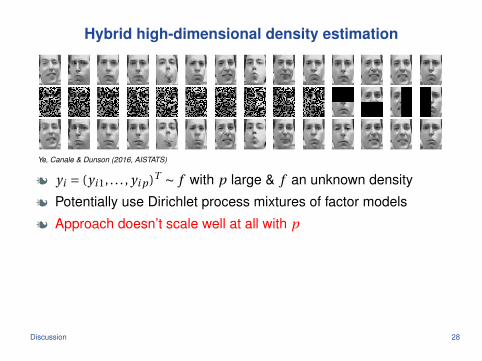
Hybrid high-dimensional density estimation
Ye, Canale & Dunson (2016, AISTATS)
j yi = (yi 1, . . . , yi p )T ∼ f with p large & f an unknown density
j Potentially use Dirichlet process mixtures of factor models
j Approach doesn’t scale well at all with p
j Instead use hybrid of Gibbs sampling & fast multiscale SVD
j Scalable, excellent mixing & empirical/predictive performance
Discussion 28

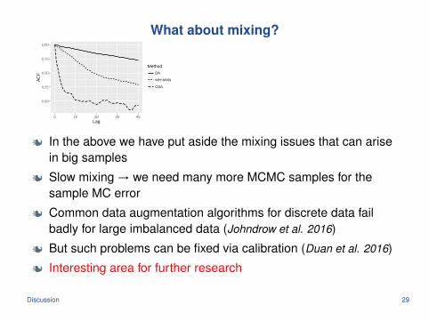
What about mixing?
0.00
0.25
0.50
0.75
1.00
0 10 20 30 40Lag
AC
F
Method
DA
MH−MVN
CDA
j In the above we have put aside the mixing issues that can arisein big samples
j Slow mixing → we need many more MCMC samples for thesample MC error
j Common data augmentation algorithms for discrete data failbadly for large imbalanced data (Johndrow et al. 2016)
j But such problems can be fixed via calibration (Duan et al. 2016)
j Interesting area for further research
Discussion 29

Primary References
j Duan L, Johndrow J, Dunson DB (2017) Calibrated dataaugmentation for scalable Markov chain Monte Carlo.arXiv:1703.03123.
j Johndrow J, Mattingly J, Mukherjee S, Dunson DB (2015)Approximations of Markov chains and Bayesian inference.arXiv:1508.03387.
j Johndrow J, Smith A, Pillai N, Dunson DB (2016) Inefficiency ofdata augmentation for large sample imbalanced data.arXiv:1605.05798.
j Li C, Srivastava S, Dunson DB (2016) Simple, scalable andaccurate posterior interval estimation. arXiv:1605.04029;Biometrika, in press.
Discussion 30