Scaling up Bayesian Inference David Dunson Departments of Statistical Science, Mathematics & ECE, Duke University May 1, 2017

Welcome message from author
This document is posted to help you gain knowledge. Please leave a comment to let me know what you think about it! Share it to your friends and learn new things together.
Transcript

Scaling up Bayesian Inference
David Dunson
Departments of Statistical Science, Mathematics & ECE, Duke University
May 1, 2017

Outline
Motivation & background
EP-MCMC
aMCMC
Discussion
Motivation & background 2

Complex & high-dimensional data
j Interest in developing new methods for analyzing & interpretingcomplex, high-dimensional data
j Arise routinely in broad fields of sciences, engineering & evenarts & humanities
j Despite huge interest in big data, there are vast gaps that havefundamentally limited progress in many fields
Motivation & background 2

‘Typical’ approaches to big data
j There is an increasingly immense literature focused on big data
j Most of the focus has been on optimization-style methods
j Rapidly obtaining a point estimate even when sample size n &overall ‘size’ of data is immense
j Bandwagons: many people work on quite similar problems,while critical open problems remain untouched
Motivation & background 3

My focus - probability models
j General probabilistic inferencealgorithms for complex data
j We would like to be able to handlearbitrarily complex probability models
j Algorithms scalable to huge data -potentially using many computers
j Accurate uncertainty quantification (UQ) is a critical issue
j Robustness of inferences also crucial
j Particular emphasis on scientific applications - limited labeleddata
Motivation & background 4

Bayes approaches
j Bayesian methods offer an attractive general approach formodeling complex data
j Choosing a prior π(θ) & likelihood L(Y (n)|θ), the posterior is
πn(θ|Y (n)) = π(θ)L(Y (n)|θ)∫π(θ)L(Y (n)|θ)dθ
= π(θ)L(Y (n)|θ)
L(Y (n)).
j Often θ is moderate to high-dimensional & the integral in thedenominator is intractable
j Accurate analytic approximations to the posterior have provenelusive outside of narrow settings
j Markov chain Monte Carlo (MCMC) & other posterior samplingalgorithms remain the standard
j Scaling MCMC to big & complex settings challenging
Motivation & background 5
Bayes approaches
j Bayesian methods offer an attractive general approach formodeling complex data
j Choosing a prior π(θ) & likelihood L(Y (n)|θ), the posterior is
πn(θ|Y (n)) = π(θ)L(Y (n)|θ)∫π(θ)L(Y (n)|θ)dθ
= π(θ)L(Y (n)|θ)
L(Y (n)).
j Often θ is moderate to high-dimensional & the integral in thedenominator is intractable
j Accurate analytic approximations to the posterior have provenelusive outside of narrow settings
j Markov chain Monte Carlo (MCMC) & other posterior samplingalgorithms remain the standard
j Scaling MCMC to big & complex settings challengingMotivation & background 5

MCMC & Computational bottlenecks
j MCMC constructs Markov chain with stationary distributionπn(θ|Y (n))
j A transition kernel is carefully chosen & iterative samplingproceeds
j Time per iteration increases with # of parameters/unknowns
j Mixing worse as dimension of data increases
j Storing & basic processing on big data sets is problematic
j Usually multiple likelihood and/or gradient evaluations at eachiteration
Motivation & background 6

Solutions
j Embarrassingly parallel (EP) MCMC: run MCMC in parallel fordifferent subsets of data & combine.
j Approximate MCMC: Approximate expensive to evaluatetransition kernels.
j Hybrid algorithms: run MCMC for a subset of the parameters& use a fast estimate for the others.
j Designer MCMC: define clever kernels that solve mixingproblems in high dimensions
j I’ll focus on EP-MCMC & aMCMC in remainder
Motivation & background 7

Outline
Motivation & background
EP-MCMC
aMCMC
Discussion
EP-MCMC 8

Embarrassingly parallel MCMC
j Divide large sample size n data set into many smaller data setsstored on different machines
j Draw posterior samples for each subset posterior in parallelj ‘Magically’ combine the results quickly & simply
EP-MCMC 8

Embarrassingly parallel MCMC
j Divide large sample size n data set into many smaller data setsstored on different machines
j Draw posterior samples for each subset posterior in parallel
j ‘Magically’ combine the results quickly & simply
EP-MCMC 8

Embarrassingly parallel MCMC
j Divide large sample size n data set into many smaller data setsstored on different machines
j Draw posterior samples for each subset posterior in parallelj ‘Magically’ combine the results quickly & simply
EP-MCMC 8

Toy Example: Logistic Regression
200
400
600 800
1000
1200
200
400
600 800
1000
1200
200
400
600
800
100
0
1200
1600
200
400
600
800
100
0
1600
200
400
600
800
100
0 120
0
200
400
600 800
1000 1200 200
400
600
800
1000 120
0
200
400 600
800 1000
1600
200
400
600
800
100
0
1200
1800
200
400
600
800
100
0
1200 160
0
200
400
600
800
1000
120
0
200
400
600
800
1000
120
0
1600
200
400
600 800
1000
120
0
1600
200
400
600
800
1000
1200
200
400
600
800
1000 120
0
1400
200
400
600
800
100
0
140
0
1600
200
400
600
800
100
0
1600
200
400
600
800
1000 120
0
200
400
600
800 1000
1600
200
400 600
800
1000 120
0
1600
200
400
600
800
1000
1600
200
400
600
800
1000
1200
200
400
600
800 100
0
1200
160
0
200
400 600
800
100
0 1200 1600
200
400
600 800
1000
1400
200
400
600
800
1000 120
0
1600
200
400 600
800
1000 120
0
1600
200
400
600 800
1000 1200
200
400 600
800
1000
1200
1400
200
400
600
800
1000
200
400
600
800
100
0
1400
200
400
600
800
100
0
120
0 1800
200
400
600
800 100
0
120
0 1
400
200
400
600 800
1000
1200
200
400
600
800 1000
120
0
1600
200
400
600
800
1000
1200
140
0
200
400
600
800
1000
1200
200
400
600
800
1000
120
0 1600
200
400
600
800 1000 1400
200
400
600
800
1000 120
0
1800
200
400
600
800
1000
120
0
1800
−1.15 −1.10 −1.05 −1.00 −0.95 −0.90 −0.850.85
0.90
0.95
1.00
1.05
1.10
1.15
200
400
600
800
1000 120
0
500
1000
1500
2000
MCMCSubset PosteriorWASP
β1
β 2
pr(yi = 1|xi 1, . . . , xi p ,θ) =exp
(∑pj=1 xi jβ j
)1+exp
(∑pj=1 xi jβ j
) .
j Subset posteriors: ‘noisy’ approximations of full data posterior.
j ‘Averaging’ of subset posteriors reduces this ‘noise’ & leads toan accurate posterior approximation.
EP-MCMC 9

Toy Example: Logistic Regression
200
400
600 800
1000
1200
200
400
600 800
1000
1200
200
400
600
800
100
0
1200
1600
200
400
600
800
100
0
1600
200
400
600
800
100
0 120
0
200
400
600 800
1000 1200 200
400
600
800
1000 120
0
200
400 600
800 1000
1600
200
400
600
800
100
0
1200
1800
200
400
600
800
100
0
1200 160
0
200
400
600
800
1000
120
0
200
400
600
800
1000
120
0
1600
200
400
600 800
1000
120
0
1600
200
400
600
800
1000
1200
200
400
600
800
1000 120
0
1400
200
400
600
800
100
0
140
0
1600
200
400
600
800
100
0
1600
200
400
600
800
1000 120
0
200
400
600
800 1000
1600
200
400 600
800
1000 120
0
1600
200
400
600
800
1000
1600
200
400
600
800
1000
1200
200
400
600
800 100
0
1200
160
0
200
400 600
800
100
0 1200 1600
200
400
600 800
1000
1400
200
400
600
800
1000 120
0
1600
200
400 600
800
1000 120
0
1600
200
400
600 800
1000 1200
200
400 600
800
1000
1200
1400
200
400
600
800
1000
200
400
600
800
100
0
1400
200
400
600
800
100
0
120
0 1800
200
400
600
800 100
0
120
0 1
400
200
400
600 800
1000
1200
200
400
600
800 1000
120
0
1600
200
400
600
800
1000
1200
140
0
200
400
600
800
1000
1200
200
400
600
800
1000
120
0 1600
200
400
600
800 1000 1400
200
400
600
800
1000 120
0
1800
200
400
600
800
1000
120
0
1800
−1.15 −1.10 −1.05 −1.00 −0.95 −0.90 −0.850.85
0.90
0.95
1.00
1.05
1.10
1.15
200
400
600
800
1000 120
0
500
1000
1500
2000
MCMCSubset PosteriorWASP
β1
β 2
pr(yi = 1|xi 1, . . . , xi p ,θ) =exp
(∑pj=1 xi jβ j
)1+exp
(∑pj=1 xi jβ j
) .
j Subset posteriors: ‘noisy’ approximations of full data posterior.j ‘Averaging’ of subset posteriors reduces this ‘noise’ & leads to
an accurate posterior approximation.EP-MCMC 9
Stochastic Approximation
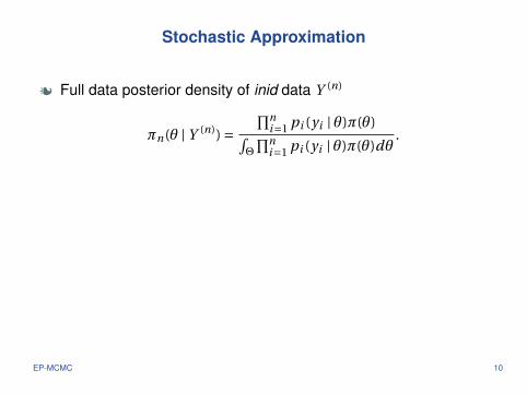
j Full data posterior density of inid data Y (n)
πn(θ | Y (n)) =∏n
i=1 pi (yi | θ)π(θ)∫Θ
∏ni=1 pi (yi | θ)π(θ)dθ
.
j Divide full data Y (n) into k subsets of size m:Y (n) = (Y[1], . . . ,Y[ j ], . . . ,Y[k]).
j Subset posterior density for j th data subset
πγm(θ | Y[ j ]) =
∏i∈[ j ](pi (yi | θ))γπ(θ)∫
Θ
∏i∈[ j ](pi (yi | θ))γπ(θ)dθ
.
j γ=O(k) - chosen to minimize approximation error
EP-MCMC 10

Stochastic Approximation
j Full data posterior density of inid data Y (n)
πn(θ | Y (n)) =∏n
i=1 pi (yi | θ)π(θ)∫Θ
∏ni=1 pi (yi | θ)π(θ)dθ
.
j Divide full data Y (n) into k subsets of size m:Y (n) = (Y[1], . . . ,Y[ j ], . . . ,Y[k]).
j Subset posterior density for j th data subset
πγm(θ | Y[ j ]) =
∏i∈[ j ](pi (yi | θ))γπ(θ)∫
Θ
∏i∈[ j ](pi (yi | θ))γπ(θ)dθ
.
j γ=O(k) - chosen to minimize approximation error
EP-MCMC 10

Barycenter in Metric Spaces
EP-MCMC 11

Barycenter in Metric Spaces
EP-MCMC 12

WAsserstein barycenter of Subset Posteriors (WASP)
Srivastava, Li & Dunson (2015)
j 2-Wasserstein distance between µ,ν ∈P 2(Θ)
W2(µ,ν) = inf{(E[d 2(X ,Y )]
) 12 : law(X ) =µ, law(Y ) = ν
}.
j Πγm(· | Y[ j ]) for j = 1, . . . ,k are combined through WASP
Πγn(· | Y (n)) = argmin
Π∈P 2(Θ)
1
k
k∑j=1
W 22 (Π,Πγ
m(· | Y[ j ])). [Agueh & Carlier (2011)]
j Plugging in Π̂γm(· | Y[ j ]) for j = 1, . . . ,k, a linear program (LP) can
be used for fast estimation of an atomic approximation
EP-MCMC 13

LP Estimation of WASP
j Minimizing Wasserstein is solution to a discrete optimaltransport problem
j Let µ=∑J1j=1 a jδθ1 j , ν=∑J2
l=1 blδθ2l & M12 ∈ℜJ1×J2 = matrix ofsquare differences in atoms {θ1 j }, {θ2l }.
j Optimal transport polytope: T (a,b) = set of doubly stochasticmatrices w/ row sums a & column sums b
j Objective is to find T ∈T (a,b) minimizing tr(TT M12)
j For WASP, generalize to multimargin optimal transport problem- entropy smoothing has been used previously
j We can avoid such smoothing & use sparse LP solvers -neglible computation cost compared to sampling
EP-MCMC 14

WASP: Theorems
Theorem (Subset Posteriors)Under “usual” regularity conditions, there exists a constant C1
independent of subset posteriors, such that for large m,
EP [ j ]θ0
W 22
{Πγm(· | Y[ j ]),δθ0 (·)}≤C1
(log2 m
m
) 1α
j = 1, . . . ,k,
Theorem (WASP)Under “usual” regularity conditions and for large m,
W2
{Πγn(· | Y (n)),δθ0 (·)
}=OP (n)
θ0
√log2/αm
km1/α
.
EP-MCMC 15

Simple & Fast Posterior Interval Estimation (PIE)
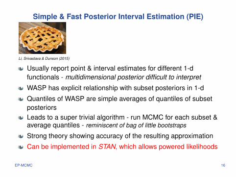
Li, Srivastava & Dunson (2015)
j Usually report point & interval estimates for different 1-dfunctionals - multidimensional posterior difficult to interpret
j WASP has explicit relationship with subset posteriors in 1-d
j Quantiles of WASP are simple averages of quantiles of subsetposteriors
j Leads to a super trivial algorithm - run MCMC for each subset &average quantiles - reminiscent of bag of little bootstraps
j Strong theory showing accuracy of the resulting approximation
j Can be implemented in STAN, which allows powered likelihoods
EP-MCMC 16

Simple & Fast Posterior Interval Estimation (PIE)
Li, Srivastava & Dunson (2015)
j Usually report point & interval estimates for different 1-dfunctionals - multidimensional posterior difficult to interpret
j WASP has explicit relationship with subset posteriors in 1-d
j Quantiles of WASP are simple averages of quantiles of subsetposteriors
j Leads to a super trivial algorithm - run MCMC for each subset &average quantiles - reminiscent of bag of little bootstraps
j Strong theory showing accuracy of the resulting approximation
j Can be implemented in STAN, which allows powered likelihoods
EP-MCMC 16

Theory on PIE/1-d WASP
j We show 1-d WASP Πn(ξ|Y (n)) is highly accurate approximationto exact posterior Πn(ξ|Y (n))
j As subset sample size m increases, W2 distance between themdecreases at faster than parametric rate op (n−1/2)
j Theorem allows k =O(nc ) and m =O(n1−c ) for any c ∈ (0,1), som can increase very slowly relative to k (recall n = mk)
j Their biases, variances, quantiles only differ in high orders ofthe total sample size
j Conditions: standard, mild conditions on likelihood + prior finite2nd moment & uniform integrabiity of subset posteriors
EP-MCMC 17
Results
j We have implemented for rich variety of data & models
j Logistic & linear random effects models, mixture models, matrix& tensor factorizations, Gaussian process regression
j Nonparametric models, dependence, hierarchical models, etc.
j We compare to long runs of MCMC (when feasible) & VB
j WASP/PIE is much faster than MCMC & highly accurate
j Carefully designed VB implementations often do very well
EP-MCMC 18

Outline
Motivation & background
EP-MCMC
aMCMC
Discussion
aMCMC 19

aMCMC Johndrow, Mattingly, Mukherjee & Dunson (2015)
j Different way to speed up MCMC - replace expensive transitionkernels with approximations
j For example, approximate a conditional distribution in Gibbssampler with a Gaussian or using a subsample of data
j Can potentially vastly speed up MCMC sampling inhigh-dimensional settings
j Original MCMC sampler converges to a stationary distributioncorresponding to the exact posterior
j Not clear what happens when we start substituting inapproximations - may diverge etc
aMCMC 19

aMCMC Overview
j aMCMC is used routinely in an essentially ad hoc manner
j Our goal: obtain theory guarantees & use these to target designof algorithms
j Define ‘exact’ MCMC algorithm, which is computationallyintractable but has good mixing
j ‘exact’ chain converges to stationary distribution correspondingto exact posterior
j Approximate kernel in exact chain with more computationallytractable alternative
aMCMC 20

Sketch of theory
j Define sε = τ1(P )/τ1(Pε) = computational speed-up, τ1(P ) =time for one step with transition kernel P
j Interest: optimizing computational time-accuracy tradeoff forestimators of Π f = ∫
Θ f (θ)Π(dθ|x)
j We provide tight, finite sample bounds on L2 error
j aMCMC estimators win for low computational budgets but haveasymptotic bias
j Often larger approximation error → larger sε & rougherapproximations are better when speed super important
aMCMC 21

Ex 1: Approximations using subsets
j Replace the full data likelihood with
Lε(x | θ) =(∏
i∈VL(xi | θ)
)N /|V |,
for randomly chosen subset V ⊂ {1, . . . ,n}.
j Applied to Pólya-Gamma data augmentation for logisticregression
j Different V at each iteration – trivial modification to Gibbsj Assumptions hold with high probability for subsets > minimal
size (wrt distribution of subsets, data & kernel).
aMCMC 22

Ex 1: Approximations using subsets
j Replace the full data likelihood with
Lε(x | θ) =(∏
i∈VL(xi | θ)
)N /|V |,
for randomly chosen subset V ⊂ {1, . . . ,n}.j Applied to Pólya-Gamma data augmentation for logistic
regression
j Different V at each iteration – trivial modification to Gibbsj Assumptions hold with high probability for subsets > minimal
size (wrt distribution of subsets, data & kernel).
aMCMC 22

Ex 1: Approximations using subsets
j Replace the full data likelihood with
Lε(x | θ) =(∏
i∈VL(xi | θ)
)N /|V |,
for randomly chosen subset V ⊂ {1, . . . ,n}.j Applied to Pólya-Gamma data augmentation for logistic
regressionj Different V at each iteration – trivial modification to Gibbs
j Assumptions hold with high probability for subsets > minimalsize (wrt distribution of subsets, data & kernel).
aMCMC 22

Ex 1: Approximations using subsets
j Replace the full data likelihood with
Lε(x | θ) =(∏
i∈VL(xi | θ)
)N /|V |,
for randomly chosen subset V ⊂ {1, . . . ,n}.j Applied to Pólya-Gamma data augmentation for logistic
regressionj Different V at each iteration – trivial modification to Gibbsj Assumptions hold with high probability for subsets > minimal
size (wrt distribution of subsets, data & kernel).aMCMC 22

Application to SUSY dataset
j n = 5,000,000 (0.5 million test), binary outcome & 18 continuouscovariates
j Considered subsets sizes ranging from |V | = 1,000 to 4,500,000
j Considered different losses as function of |V |j Rate at which loss → 0 with ε heavily dependent on loss
j For small computational budget & focus on posterior meanestimation, small subsets preferred
j As budget increases & loss focused more on tails (e.g., forinterval estimation), optimal |V | increases
aMCMC 23

Application to SUSY dataset
j n = 5,000,000 (0.5 million test), binary outcome & 18 continuouscovariates
j Considered subsets sizes ranging from |V | = 1,000 to 4,500,000
j Considered different losses as function of |V |
j Rate at which loss → 0 with ε heavily dependent on loss
j For small computational budget & focus on posterior meanestimation, small subsets preferred
j As budget increases & loss focused more on tails (e.g., forinterval estimation), optimal |V | increases
aMCMC 23

Application to SUSY dataset
j n = 5,000,000 (0.5 million test), binary outcome & 18 continuouscovariates
j Considered subsets sizes ranging from |V | = 1,000 to 4,500,000
j Considered different losses as function of |V |j Rate at which loss → 0 with ε heavily dependent on loss
j For small computational budget & focus on posterior meanestimation, small subsets preferred
j As budget increases & loss focused more on tails (e.g., forinterval estimation), optimal |V | increases
aMCMC 23

Application to SUSY dataset
j n = 5,000,000 (0.5 million test), binary outcome & 18 continuouscovariates
j Considered subsets sizes ranging from |V | = 1,000 to 4,500,000
j Considered different losses as function of |V |j Rate at which loss → 0 with ε heavily dependent on loss
j For small computational budget & focus on posterior meanestimation, small subsets preferred
j As budget increases & loss focused more on tails (e.g., forinterval estimation), optimal |V | increases
aMCMC 23
Application 2: Mixture models & tensor factorizations
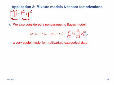
j We also considered a nonparametric Bayes model:
pr(yi 1 = c1, . . . , yi p = cp ) =k∑
h=1λh
p∏j=1
ψ( j )hc j
,
a very useful model for multivariate categorical data
j Dunson & Xing (2009) - a data augmentation Gibbs samplerj Sampling latent classes computationally prohibitive for huge n
j Use adaptive Gaussian approximation - avoid samplingindividual latent classes
j We have shown Assumptions 1-2, Assumption 2 result moregeneral than this setting
j Improved computation performance for large n
aMCMC 24

Application 2: Mixture models & tensor factorizations
j We also considered a nonparametric Bayes model:
pr(yi 1 = c1, . . . , yi p = cp ) =k∑
h=1λh
p∏j=1
ψ( j )hc j
,
a very useful model for multivariate categorical dataj Dunson & Xing (2009) - a data augmentation Gibbs sampler
j Sampling latent classes computationally prohibitive for huge n
j Use adaptive Gaussian approximation - avoid samplingindividual latent classes
j We have shown Assumptions 1-2, Assumption 2 result moregeneral than this setting
j Improved computation performance for large n
aMCMC 24

Application 2: Mixture models & tensor factorizations
j We also considered a nonparametric Bayes model:
pr(yi 1 = c1, . . . , yi p = cp ) =k∑
h=1λh
p∏j=1
ψ( j )hc j
,
a very useful model for multivariate categorical dataj Dunson & Xing (2009) - a data augmentation Gibbs samplerj Sampling latent classes computationally prohibitive for huge n
j Use adaptive Gaussian approximation - avoid samplingindividual latent classes
j We have shown Assumptions 1-2, Assumption 2 result moregeneral than this setting
j Improved computation performance for large n
aMCMC 24

Application 3: Low rank approximation to GP
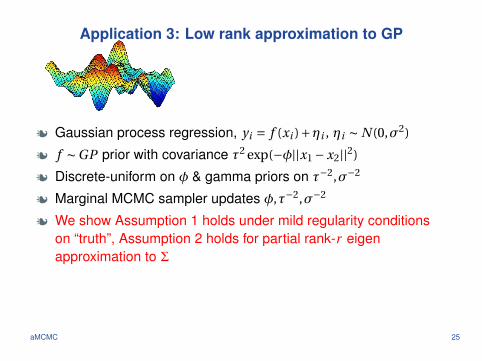
j Gaussian process regression, yi = f (xi )+ηi , ηi ∼ N (0,σ2)
j f ∼GP prior with covariance τ2 exp(−φ||x1 −x2||2)
j Discrete-uniform on φ & gamma priors on τ−2,σ−2
j Marginal MCMC sampler updates φ,τ−2,σ−2
j We show Assumption 1 holds under mild regularity conditionson “truth”, Assumption 2 holds for partial rank-r eigenapproximation to Σ
j Less accurate approximations clearly superior in practice forsmall computational budget
aMCMC 25

Application 3: Low rank approximation to GP
j Gaussian process regression, yi = f (xi )+ηi , ηi ∼ N (0,σ2)
j f ∼GP prior with covariance τ2 exp(−φ||x1 −x2||2)
j Discrete-uniform on φ & gamma priors on τ−2,σ−2
j Marginal MCMC sampler updates φ,τ−2,σ−2
j We show Assumption 1 holds under mild regularity conditionson “truth”, Assumption 2 holds for partial rank-r eigenapproximation to Σ
j Less accurate approximations clearly superior in practice forsmall computational budget
aMCMC 25

Applications: General Conclusions
j Achieving uniform control of approximation error ε requiresapproximations adaptive to current state of chain
j More accurate approximations needed farther from highprobability region of posterior; good as chain rarely there
j Approximations to conditionals of vector parameters are highlysensitive to 2nd moment
j Smaller condition numbers for the covariance matrix of vectorparameters mean less accurate approximations can be used
aMCMC 26

Outline
Motivation & background
EP-MCMC
aMCMC
Discussion
Discussion 27
Discussion
j Proposed very general classes of scalable Bayes algorithms
j EP-MCMC & aMCMC - fast & scalable with guarantees
j Interest in improving theory - avoid reliance on asymptotics inEP-MCMC & weaken assumptions in aMCMC
j Useful to combine algorithms - e.g., run aMCMC for each subset
j By looking at algorithms through our theory lens, suggests new& improved algorithms
j Also, very interested in hybrid frequentist-Bayes algorithms
Discussion 27

Hybrid high-dimensional density estimation
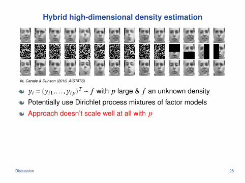
Ye, Canale & Dunson (2016, AISTATS)
j yi = (yi 1, . . . , yi p )T ∼ f with p large & f an unknown density
j Potentially use Dirichlet process mixtures of factor models
j Approach doesn’t scale well at all with p
j Instead use hybrid of Gibbs sampling & fast multiscale SVD
j Scalable, excellent mixing & empirical/predictive performance
Discussion 28

Hybrid high-dimensional density estimation
Ye, Canale & Dunson (2016, AISTATS)
j yi = (yi 1, . . . , yi p )T ∼ f with p large & f an unknown density
j Potentially use Dirichlet process mixtures of factor models
j Approach doesn’t scale well at all with p
j Instead use hybrid of Gibbs sampling & fast multiscale SVD
j Scalable, excellent mixing & empirical/predictive performance
Discussion 28

What about mixing?
0.00
0.25
0.50
0.75
1.00
0 10 20 30 40Lag
AC
F
Method
DA
MH−MVN
CDA
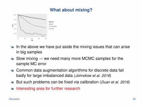
j In the above we have put aside the mixing issues that can arisein big samples
j Slow mixing → we need many more MCMC samples for thesample MC error
j Common data augmentation algorithms for discrete data failbadly for large imbalanced data (Johndrow et al. 2016)
j But such problems can be fixed via calibration (Duan et al. 2016)
j Interesting area for further research
Discussion 29

What about mixing?
0.00
0.25
0.50
0.75
1.00
0 10 20 30 40Lag
AC
F
Method
DA
MH−MVN
CDA
j In the above we have put aside the mixing issues that can arisein big samples
j Slow mixing → we need many more MCMC samples for thesample MC error
j Common data augmentation algorithms for discrete data failbadly for large imbalanced data (Johndrow et al. 2016)
j But such problems can be fixed via calibration (Duan et al. 2016)
j Interesting area for further research
Discussion 29

Primary References
j Duan L, Johndrow J, Dunson DB (2017) Calibrated dataaugmentation for scalable Markov chain Monte Carlo.arXiv:1703.03123.
j Johndrow J, Mattingly J, Mukherjee S, Dunson DB (2015)Approximations of Markov chains and Bayesian inference.arXiv:1508.03387.
j Johndrow J, Smith A, Pillai N, Dunson DB (2016) Inefficiency ofdata augmentation for large sample imbalanced data.arXiv:1605.05798.
j Li C, Srivastava S, Dunson DB (2016) Simple, scalable andaccurate posterior interval estimation. arXiv:1605.04029;Biometrika, in press.
Discussion 30
Related Documents