XYZ Real Estate Fund, LP
REIS Performance
Measurement Resource
Manual
This Real Estate Information Standards (REIS) Manual has been developed with participation from NCREIF’s Performance Measurement Committee. The Manual has been endorsed by the REIS Council and approved for publication by the REIS Board.
As approved by the REIS Board on December 11, 2012
67
Real Estate Information Standards Handbook Volume II 68
Contents
Introduction 69
Time-weighted returns 71
Money-weighted returns (IRRs) 90
Equity multiples 94
Other performance metrics 97
Performance attribution 106
Computation methodologies 108
Sample disclosures 113
Performance measurement information elements 117
Appendices 119
Appendix A — Sample Fund Level Presentation for Client Reporting 120
Appendix B — Sample Property Level Presentation for Client Reporting 121
Introduction
Real Estate Information Standards Handbook Volume II 69
Introduction
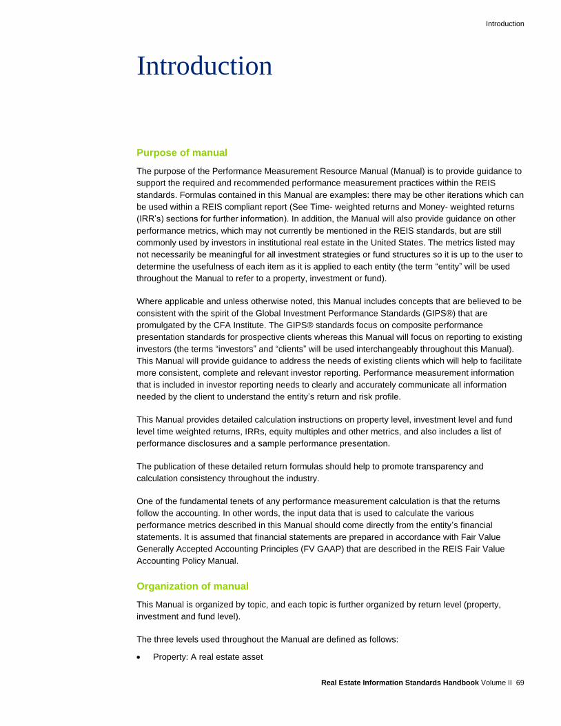
Purpose of manual
The purpose of the Performance Measurement Resource Manual (Manual) is to provide guidance to
support the required and recommended performance measurement practices within the REIS
standards. Formulas contained in this Manual are examples: there may be other iterations which can
be used within a REIS compliant report (See Time- weighted returns and Money- weighted returns
(IRR’s) sections for further information). In addition, the Manual will also provide guidance on other
performance metrics, which may not currently be mentioned in the REIS standards, but are still
commonly used by investors in institutional real estate in the United States. The metrics listed may
not necessarily be meaningful for all investment strategies or fund structures so it is up to the user to
determine the usefulness of each item as it is applied to each entity (the term “entity” will be used
throughout the Manual to refer to a property, investment or fund).
Where applicable and unless otherwise noted, this Manual includes concepts that are believed to be
consistent with the spirit of the Global Investment Performance Standards (GIPS®) that are
promulgated by the CFA Institute. The GIPS® standards focus on composite performance
presentation standards for prospective clients whereas this Manual will focus on reporting to existing
investors (the terms “investors” and “clients” will be used interchangeably throughout this Manual).
This Manual will provide guidance to address the needs of existing clients which will help to facilitate
more consistent, complete and relevant investor reporting. Performance measurement information
that is included in investor reporting needs to clearly and accurately communicate all information
needed by the client to understand the entity’s return and risk profile.
This Manual provides detailed calculation instructions on property level, investment level and fund
level time weighted returns, IRRs, equity multiples and other metrics, and also includes a list of
performance disclosures and a sample performance presentation.
The publication of these detailed return formulas should help to promote transparency and
calculation consistency throughout the industry.
One of the fundamental tenets of any performance measurement calculation is that the returns
follow the accounting. In other words, the input data that is used to calculate the various
performance metrics described in this Manual should come directly from the entity’s financial
statements. It is assumed that financial statements are prepared in accordance with Fair Value
Generally Accepted Accounting Principles (FV GAAP) that are described in the REIS Fair Value
Accounting Policy Manual.
Organization of manual
This Manual is organized by topic, and each topic is further organized by return level (property,
investment and fund level).
The three levels used throughout the Manual are defined as follows:
Property: A real estate asset

Introduction
Real Estate Information Standards Handbook Volume II 70
Investment: A discrete asset or group of assets held for income, appreciation, or both and
tracked separately (primarily reflects the investor’s economic ownership interest).
Fund: A fund has one or more investments and includes all commingled funds and single client
accounts. Please note that this term is applied more broadly in this Manual than it is in the
NCREIF5/Townsend Fund Indices which do not include single client accounts in their definition.
The use of the term is consistent with the REIS standards.
The detailed return formulas included in the Manual can generally be found in two separate places.
First, the formulas are included in the text of the Manual with the specific topic they are covering.
This allows the user to view each topic as a stand-alone section, and not have to turn to other
sections for the details. Secondly, all the formulas have been compiled in the section labeled
“Computation Methodologies”.
The sample presentations (Appendix A and B) and sample disclosures that are included in the
Manual are intended for illustrative purposes only and are not meant to reflect the only correct
presentation for these items.
The section labeled “Performance Measurement Information Elements” includes a list of the financial
elements that should be collected and retained by information providers as these elements are
commonly used in the various return formulas.
This Manual will be reviewed annually for potential updates.
5 The National Council of Real Estate Fiduciaries (“NCREIF”) is a co-sponsor of the Real Estate Information Standards.
www.ncreif.org

Time-weighted returns
Real Estate Information Standards Handbook Volume II 71
Time-weighted returns
Overview of TWR
Definition
A time-weighted return (TWR) can be defined as the geometric average of the holding period yields
to an investment portfolio6. TWRs are commonly used in the investment industry to measure the
performance of an investment manager. The TWR formulas isolate the performance of the
investment earned by removing the timing effect of cash contributions and distributions from the
investment’s ending fair value. In other words, TWRs measure how well a manager performed over
the measurement period regardless of the size of the investment or timing of external cash flows.
All TWR formulas are built in a similar manner, with a numerator and denominator that result in a
percentage return. The numerators generally represent some measure of the absolute performance
of the entity over the measurement period (quarterly NOI, monthly appreciation, etc.). The
denominators represent a measure of the entity’s average size over that same time period (average
fair value of real estate, weighted average net asset value, etc.). In the most general terms, a TWR
can be calculated for just about any time period (day, month, quarter, year, etc.), using discrete sub-
periods as building blocks for the entire measurement period. For example, a five-year TWR can be
calculated by linking either five annual TWR calculations or twenty quarterly TWR calculations. In
practical terms, the quarter is used as the building block for most real estate TWR calculations and
the linking of these building blocks is described further below.Note that industry practice may use
TWR formulas with different periodicity and varying conventions regarding capital transactions and
distributions which may result in modest return variations. Within a REIS compliant report, these
variations are acceptable; however the minimum periodicity is quarterly.
A technical point worth remembering: “Time-weighting” refers to the process of how multiple periodic
rates of return are linked together. Hence, the rate of return for a single period should not technically
be referred to as a time-weighted rate of return. In fact, the popular Modified Dietz method, which is
the basis for the single period rate of return used in real estate, is an approximate IRR computation
for that calendar quarter. It is the chain-linking of such quarterly Modified Dietz returns, a process
that affords each quarterly rate of return an equal weight (rather than a weight which is also
proportional to the number of dollars invested), that results in a (multi-period) “time-weighted” rate of
return.
Use of TWRs
TWRs are the preferred performance measure to use when a manager does not have control over
the cash flows of the investment. This lack of control is typically seen in open-end funds and non-
discretionary single client account portfolios. By removing the timing effect of cash flows from the
formulas, TWRs provide a good measure of the manager’s ability to manage an entity according to a
specified strategy or objective. In addition, TWRs are preferred when valuation frequency is high and
6 Investment Analysis and Portfolio Management, Seventh Edition (2003)

Time-weighted returns
Real Estate Information Standards Handbook Volume II 72
returns are linear, and when one needs to compare performance across multiple asset classes or
industry benchmarks that are primarily TWR based. Conversely, when a manager does control the
cash flows of the entity, as is the case in a closed-end fund or discretionary single client account
portfolio, other return measures including IRRs may provide additional insight.
Within the industry, TWRs are calculated at three “levels”: property, investment and fund.
Regardless of the level, the TWRs all follow the same basic application principles that are described
below. The actual financial elements that are used in the numerators and denominators of each
TWR differ by level and are described in greater detail in later sections.
Industry practice is to separate the total return into its two components, income return and
appreciation return, for certain strategies. The REIS standards require fund level component TWRs
for all funds.
Modified Dietz Method
The Modified-Dietz Method is the single period rate of return formula that is widely used throughout
the financial industry to combine into TWRs. When someone refers to a “time-weighted return
formula” in general terms, they are most likely referring to a linking of periodic rates of return that
each use the formula below.
Rp = EFV — BFV — CF
BFV + WCF
Rp = Return for the measurement period
EFV = Ending fair value of the investment
BFV = Beginning fair value of the investment
CF = Net cash flows for the period (add if net distribution)
WCF = Sum of weighted cash flows for the period
Ideally, a time-weighted return involves breaking the holding period into sub-periods bounded by
each subsequent cash flow, then chain-linking the sub-period TWRs. By valuing the portfolio at the
instant just prior to any cash flow, the sub-period return for the time period leading up to that cash
flow occurrence can be calculated. By then re-valuing the portfolio considering the effect of such a
cash flow, a new beginning value is created for computing the rate of return for the next sub-period.
Since there are no cash flows within these sub-periods, the sub-period TWRs are simply (ending
value — beginning value)/beginning value.
Given the computing power available nowadays, the only barrier to computing such an ‘ideal TWR’
is the availability of timely pricing, e.g., valuation information, when each cash flow occurs. For
example, in the stock market, many participants now routinely perform such ideal TWRs by using
end of day stock pricing.
However, in markets where getting pricing data is problematic, such as with real estate,
approximations are necessary. The most popular approximation for such markets is the Modified
Dietz method, a method that has its origins in an earlier place and time when, even if timely prices
were available, computing power was limited. It allows the placement of sub-period boundaries at
dates when valuation data will be available, e.g., quarterly. Within these sub-periods, if a cash flow
occurs, an implicit constant rate of return before and after is effectively assumed by time-weighting
the cash flows in the denominator by the fraction of the sub-period duration that the cash flows affect
the portfolio.
If there is a material amount of volatility in values during the sub-period or the cash flows are large,
the user should break the sub-period into two pieces, thus forcing a revaluation of the portfolio at the
breakpoint. The GIPS® standards allow users to decide their own acceptable level of precision. In

Time-weighted returns
Real Estate Information Standards Handbook Volume II 73
most markets, a cash flow greater than 10% of the pre-cash flow portfolio value is considered to
cause excess imprecision. In real estate, sub-periods are only 3 months long and thus sub-period
volatility is typically immaterial. A Modified Dietz approximation will likely be appropriate, except
when there is either a large partial sale or a single, substantial capital improvement expenditure.
Nevertheless, the GIPS® standards presently permit the real estate sector to use these quarterly
sub-periods, decide on what is precise enough and employ such a Modified Dietz approximation
within each quarter.
It is noted that the NCREIF property level return formulas are simply a slight, further approximation
of Modified Dietz methodology wherein, rather than time-tagging the cash flows to the nearest day,
contributions (for capital improvements) are assumed to always be made mid-quarter and
distributions (of NOI) are assumed to be made monthly. The NCRIEF formula is discussed as an
example; there are other time-weighted approaches that could be employed for a firm to claim REIS
compliance.
The Modified Dietz Method provides a measure of the total return for the entity over the
measurement period and is used as a building block for the more detailed formulas that are
commonly used in the industry which will be described in greater detail in later sections. Specifically
the Modified Dietz Method provides for an approximation of the IRR for the measurement period
without the need for daily valuation and return calculation. Typically, the total TWR for an entity will
more closely match the IRR in cases where there are no significant cash flows or large interim
changes in value such as in the case of a core asset. As you move further out in the risk spectrum,
the IRR and total TWR tend to be more dissimilar.
Application of TWRs
Cumulative returns
Since valuations are performed typically quarterly, and since the Modified Dietz approximation within
such a short sub-period will almost always be adequate (given the nature of real estate cash flows),
the period for computing real estate sub-period TWRs is presumed to be the quarter. Periods less
than a quarter, for instance monthly, can also be used provided the valuation cycle also occurs with
that same frequency. In the U.S., monthly valuations for private real estate are currently rare; hence
the quarter is most commonly used. Returns for periods longer than a single quarter, known as
cumulative returns (not annualized), can be calculated by geometrically linking all of the quarterly
returns within the measurement period. This geometric linking is applied uniformly to all of the
quarterly sub-periods within the cumulative period. If the user has adopted a partial period policy that
calls for including the partial periods in the calculation, then those partial periods would need to be
geometrically linked with the full quarters as well. TWRs do not require equal length sub-periods to
calculate cumulative returns correctly. For more details on partial period calculations, please refer to
the partial period issues section below. The geometrically linked calculation of TWRs results in a
compounded rate of return.
Rp = (1 +R1) * (1+R2) * (1+R3)…(1+Rn)] — 1
Rp = Return for the measurement period
R1…n = Quarterly return for period 1 through n
In the geometrically linked cumulative return formula above, each quarterly return in the
measurement period has an equal weighting. The timing of the return and the amount invested for
an individual period will have no impact on the multi-period return. In other words, every period
counts as much as every other period, regardless of the entity’s size in a TWR.

Time-weighted returns
Real Estate Information Standards Handbook Volume II 74
An example of an eight quarter cumulative return is included below. Please note that arithmetic
return for this period would be 20%, (2.5% * 8), however the compounding effect introduced by
geometrically linking the returns results in an additional 1.8% of return for an ending value of 21.8%.
Cumulative return example (not annualized)
Return (Return) + 1
Start Quarter 1 2.5% 1.025
Quarter 2 2.5% 1.025
Quarter 3 2.5% 1.025
Quarter 4 2.5% 1.025
Quarter 5 2.5% 1.025
Quarter 6 2.5% 1.025
Quarter 7 2.5% 1.025
End Quarter 8 2.5% 1.025
Cumulative return 21.8%
[(1.025)*(1.025)*(1.025)*(1.025)*(1.025)*(1.025)*(1.025)*(1.025)]-1 = .218 = 21.8%
Annualization
In the financial industry, investors and managers tend to think in terms of annual rates of return. The
industry standard is to annualize all cumulative returns that contain four or more full quarters.
Cumulative returns can be annualized using the following formula:
ARp = [(1 +Rp)^(365/DHP)] — 1
ARp = Annualized return for the measurement period
Rp = Return for the measurement period (non-annualized)
DHP = Number of days in the measurement period
The annualization factor shown in the formula above uses number of days in the measurement
period. If all of the sub-periods are full quarters or full months, then it is also acceptable to use
(4/Number of quarter in the measurement period) or (12/Number of months in the measurement
period), respectively. For example, the NCREIF NPI, NCREIF NFI-ODCE and NCREIF/Townsend
Fund Level Indices use 4/Number of quarters. Using number of months or quarters may give a
slightly different result than if total number of days is used, but the differences are usually
immaterial.
Annual returns that cover more than one year (e.g. a five year return) represent the average annual
return over the cumulative period. An example of an eight quarter cumulative annualized return
using the same 2.5% quarter return that was seen in the previous example is included below.
Cumulative return example (annualized)
Return (Return) + 1
Start 1/1/2006 Quarter 1 2.5% 1.025
Quarter 2 2.5% 1.025
Quarter 3 2.5% 1.025
Quarter 4 2.5% 1.025
Quarter 5 2.5% 1.025
Quarter 6 2.5% 1.025
Quarter 7 2.5% 1.025

Time-weighted returns
Real Estate Information Standards Handbook Volume II 75
Cumulative return example (annualized)
End 12/31/2007 Quarter 8 2.5% 1.025
# Days 730
Annualized cumulative return 10.4%
{[(1.025)*(1.025)*(1.025)*(1.025)*(1.025)*(1.025)*(1.025)*(1.025)]^(365/730)}-1 = .104 = 10.4%
Grouping entities
In this Manual, the term “grouping” is used to describe the process of aggregating/disaggregating
two or more entities (properties, investments or funds) to evaluate performance using the time-
weighted return. In this sense, the grouping guidance below can be applied very broadly to any
collection of entities and is not necessarily limited to composites as described in the GIPS®
standards. As an example, client performance reporting often includes grouping of entities and the
disaggregation of portfolios by property type and geographic region.
TWR composites can be created to measure the performance of more than one entity. The
mechanics for creating such a grouping are straight-forward. First, determine which entities will be
included in the group and then compile the quarterly return numerators and denominators for all
entities. Add the numerators from each of the individual entities to create a group numerator. Add
the denominators from each of the individual entities to create a group denominator. Then divide the
group numerator by the group denominator to get the group quarterly return.
An example of a group return containing five entities is listed below.
Group return example
Numerator Denominator Return
Property A 25 500 5.0%
Property B 100 10,500 1.0%
Property C 500 14,000 3.6%
Property D 100 5,000 2.0%
Property E 275 10,000 2.8%
Group 1,000 40,000 2.5%
Group returns result in a weighted-average return based on relative entity size. In other words, the
larger an entity, the more impact it will have on the group return. Please note that the grouping
described in the example above uses the entity’s denominator to determine the weight that will be
assigned to each entity in the group. In real estate, the denominator is traditionally a weighted-
average of the entity’s size (NAV or Real Estate less debt) over the quarter. Weighting the entities
based on denominator size is believed to be the most commonly used method for grouping in the
industry and is the one that is used by the various NCREIF indices. However, the GIPS® standards
do allow an alternative method in which the entities in the calculation are asset-weighted based on
beginning-of-period values rather than the beginning-of-period plus external value method that was
described above7. Either method allowed by the GIPS® standards is acceptable for purposes of
compliance with the REIS standards, but the methodology should be disclosed in the firm’s
performance calculation methodology disclosure statement and applied consistently for all grouping
calculations.
7 CFA Institute. (2010) Global Investment Performance Standards – Guidance Statement on Calculation Methodology
www.gipsstandards.org

Time-weighted returns
Real Estate Information Standards Handbook Volume II 76
Group returns for cumulative periods should be calculated by first calculating the group return for
each individual quarter within the cumulative period and then geometrically linking those group
quarterly returns using the same methodology described in the “Cumulative Returns” section above.
Component return issues
When component returns are presented for any full individual quarter the sum of the income return
plus the appreciation return will generally equal the total return. When component returns are
geometrically linked to create cumulative compounded returns, the simple addition of the cumulative
compounded income return plus the cumulative compounded appreciation return will not usually
equal the cumulative compounded total return.
One method for dealing with this inconsistency is to calculate the component returns as explained
above and note the fact that the sum of the parts not equaling the total is normal and acceptable.
The total return is precisely correct and the income and appreciation components are
approximations. These approximations are deemed acceptable because applying the more precise
cross compounding formula to the income and appreciation component returns would make the
formulas very complex and the approximated results are not materially different.
The consistency of presentation of financial information poses another issue to consider when
analyzing component returns. Specifically, joint venture income and appreciation components can
differ depending on the accounting reporting model used for the fund. In the non-operating reporting
model, a joint venture is treated as an unconsolidated investment in a venture and only those
amounts actually distributed to the fund is considered income. Any other undistributed accrued
income as well as valuation changes will be included in appreciation. In the Operating model, the
joint venture may be consolidated and if so accrued income will be in the income component of the
return and the appreciation component will contain only valuation changes, similar to a wholly owned
property. Due to this potential inconsistency, the REIS standards require disclosure of the
accounting reporting model used by the entity to accompany any component return presentation.
Partial period issues
If an asset is acquired on a date other than the first day of a quarter, or sold on a date other than the
last, the resulting measurement period is said to be a “partial period” because the asset does not
have a full quarter’s worth of activity during that period.
These partial periods can potentially create distortions in the TWR calculations. Various factors play
a role in the distortion including; the nature of the return (single entity calculation versus group
calculation), component of the return (income versus appreciation) and time-period covered (current
quarter versus annualized return).
In practice, there are a number of different methods currently being used to deal with partial periods.
It is up to each firm to decide which method to adopt as there are pros and cons to each and the
methods that are currently used for the various NCREIF indices or recommended by the GIPS®
standards for composites may not always meet the needs of the end uses. The method chosen
should be applied consistently and properly documented in the firm’s performance measurement
disclosures.

Time-weighted returns
Real Estate Information Standards Handbook Volume II 77
The three most commonly used methods are summarized below, though other methods may also be
acceptable so long as they are applied consistently and do not materially misstate the return results.
For a more detailed discussion of partial period methodology including examples that support the
pros and cons of each method listed below, please refer to the NCREIF Discussion Paper titled
Proposed Guidance for the Calculation of Time-Weighted Returns for Partial Periods8.
Method I — Start and end dates used for TWR Calculations will match the start and end dates for
the entity’s actual life (i.e. keep partial periods).
Method II — For TWR purposes, an entity will begin on the first day of the first full quarter
following acquisition and end on the last day of the last full quarter prior to disposition (i.e. drop
partial periods).
Method III — A hybrid of Methods I and II where the start date begins on the first day of the first
full quarter following acquisition and the end date matches the actual disposition date (i.e. drop
acquisition partial period but keep disposition partial period)
If partial periods are kept in the calculation, then care must be taken to ensure that the number of
actual days in the measurement period is used correctly in the various calculations. For example, if
the acquisition partial period is kept, then the numerator of the annualization factor should be the
total number of days from the actual acquisition date (not the first day in the first full period) through
the end of the measurement period. The same holds true for any disposition partial period that is
kept.
In addition if partial periods are kept in the calculation, the cash flows that are used in the
denominator of the investment and fund level return calculations need to be weighted by the actual
number of days that were outstanding in the partial period not the normal number of days that would
be available in a full period. For example, a contribution for the first acquisition in the fund that
occurs on 2/15/xx would be weighted at 100% or 44/44 days (3/31 — 2/15 = 44), not 49% or
44/90 days (3/31 — 1/1 = 90). The same holds true in the disposition period.
The chart below lists some of the pros and cons of each of the three methods above when applied to
a single-entity calculation.
Pros Cons
Method I No adjustments to returns data is required
All since inception cumulative annualized returns for income, appreciation and total are correctly calculated
Partial period income returns appear different from a full quarter return
If net income is not earned ratably in the acquisition period, the annualization factor may not be able to correct for the distorted acquisition period returns
Method II Removes appearance of skewed quarterly income returns in the partial periods
NOI data from partial periods is not always included in performance making SI reconciliation to financials difficult. If NOI data is included in the first full period, the annualized results may be overstated.
Creates distortion in appreciation return by artificially shortening hold-period
May lead to restatement of prior quarter returns when final quarter income and appreciation is not properly accrued in the final full quarter
8 NCREIF Performance Measurement Committee. (May 2011) Proposed Guidance for the Calculation of Time-
Weighted Returns for Partial Periods www.ncreif.org/resources.aspx

Time-weighted returns
Real Estate Information Standards Handbook Volume II 78
Pros Cons
Method III Removes appearance of skewed quarterly income returns in the partial periods
Since inception cumulative annualized appreciation returns are calculated correctly
Inconsistent treatment of acquisition and disposition partial periods
NOI data from partial periods is not always included in performance making SI reconciliation difficult. If NOI data is included in the first full period, the annualized results may be overstated.
The chart below lists some of the pros and cons of each of the three methods above when applied to
a group calculation.
Pros Cons
Method I No adjustments to returns data is required
Annualization factor corrects any distortion caused by partial periods that occur in the beginning or end of a composite’s life
Partial periods that occur mid-life still distort the composite returns (income, appreciation and total)
Income returns in first/last partial period still appear different from a full period calculation
If net income is not earned ratably in the acquisition period, the annualization factor may not be able to correct for the distorted acquisition period returns
Method II Removes appearance of skewed quarterly income returns in all acquisition partial periods
Method used by NCREIF fund indices
NOI data from partial periods is not always included in performance making SI reconciliation difficult. . If NOI data is included in the first full period, the annualized results may be overstated.
Creates distortion in appreciation return by artificially shortening hold-period
May lead to restatement of prior quarter returns when final quarter income and appreciation is not properly accrued in the final full quarter
Method III Removes appearance of skewed quarterly income returns in all acquisition partial periods
Since inception cumulative annualized appreciation returns are more correct than Method B
Method used by NCREIF NPI
Inconsistent treatment of acquisition and disposition partial periods
NOI data from partial periods is not always included in performance making SI reconciliation difficult. If NOI data is included in the first full period, the annualized results may be overstated.
The treatment of partial periods by large indices may also be relevant information for users as they
decide which method to apply. However, please note that the index policy may not necessarily be
the best policy for the user because the sheer number of non-partial periods included in the index in
any given quarter will mitigate the inclusion of a few partial periods and should make any potential
distortion immaterial. Furthermore, the indices have specific inclusion requirements that may
otherwise prohibit an entity from entering the index in its acquisition period further reducing the risk
of distortion due to partial periods. In other words, this is one piece of information that the user
should consider when determining its partial period methodology but it should not be the sole
determinant. The NPI follows Method III, the NFI-ODCE follows Method II and the
NCREIF/Townsend Closed End Fund Indices also follow Method II.

Time-weighted returns
Real Estate Information Standards Handbook Volume II 79
The GIPS® standards, which are the foundational standard for performance measurement in the
REIS standards, provides the following guidance on partial periods which points toward using
Method I for composite calculations.
“When calculating time-weighted returns, for periods beginning on or after 1 January 2011, it is
recommended that real estate composites include new portfolios on the portfolio’s inception
date, which is typically the date of the portfolio’s first external cash flow. Similarly, the GIPS®
standards state that terminated portfolios must be included in the historical performance of the
composite up to the last full measurement periods that each portfolio was under management.”9
One of the stated goals of this manual is to provide guidance which will help to promote
transparency and consistency throughout the industry. Noting that firms have a choice in which
partial period methodology to apply conflicts with the latter half of this goal but we feel that it is the
best guidance given that the GIPS® standards and the NCREIF indices all point to different
methods. Furthermore, we would like to stress that the method chosen should be applied
consistently and properly documented which we believe is consistent with the spirit of the GIPS®
standards and the Manual’s goal of promoting transparency and full disclosure.
Property level TWRs
Property level TWRs reflect the performance of an operating property or group of properties. The
property level relates strictly to property operations and attempts to strip out all ownership level
activity, usually including advisory fees, use of working capital and owner income and expenses. As
such, property level TWRs do not represent investors’ earnings from those properties, even in single
property funds, but rather the earnings (in the form of appreciation and operating income) that are
generated by the property.
Leveraged vs. unleveraged
Property level TWRs can be calculated on a leveraged or unleveraged basis.
Unleveraged property level TWR
Property level TWRs are usually reported on an unleveraged basis because not all properties are
leveraged and those that are, are leveraged at varying levels which makes comparison of leveraged
returns among different properties difficult in many cases. The NCREIF Property Index (NPI) is an
unleveraged, property level index. The property level, unleveraged return formulas used by NCREIF
are as follows:
Net operating income return (unleveraged)
NOI
FVt-1 + (1/2)(CI - PSP) - (1/3)(NOI)
Appreciation return (unleveraged)
(FVt-FVt-1) + PSP - CI
FVt-1 + (1/2)(CI - PSP) - (1/3)(NOI)
9 CFA Institute. (2010) Global Investment Performance Standards – Guidance Statement on Real Estate
www.gipsstandards.org

Time-weighted returns
Real Estate Information Standards Handbook Volume II 80
Total return (unleveraged)
NOI + (FVt - FVt-1) + PSP - CI
FVt-1 + (1/2)(CI - PSP)- (1/3)(NOI)
NOI = Net operating income (before interest expense)
CI = Capital improvements
FVt = Fair value of property at end of period
FVt-1 = Fair value of property at beginning of period
PSP = Sales proceeds for partial sales (net of selling costs)
Note that all three denominators in the formulas above are the same. In addition, the total return
numerator is simply an addition of the net operating income and appreciation return numerator
components. These two observations will hold true for all component TWRs that are calculated
using the same parameters (i.e. leveraged property level, before fee investment level, etc.)
Net operating income numerator (unleveraged)
The net operating income (NOI) numerator is the net operating income (before interest expenses)
that was reported by the property during the period. The NOI should be calculated on the accrual
basis of accounting in accordance with the accounting standards explained in the REIS Fair Value
Accounting Policy Manual. Fund or investment level income and expenses should be excluded from
NOI because the property level returns focus on property operations.
Appreciation numerator (unleveraged)
The appreciation numerator measures the change in property value (increase or decrease) not
caused by capital improvements or sales. Property level financial statements should be prepared in
accordance with Fair Value Generally Accepted Accounting Principles (FV GAAP) for return
purposes and valuations should be completed on a quarterly basis in accordance with the valuation
standards outlined in the REIS standards.
Denominator (unleveraged)
Given that it is based on an approximation to IRR, the appropriate formula for the denominator of the
unleveraged property return is an estimate of the average gross capital invested in the property over
the quarter. This is calculated by adjusting the beginning real estate value of the property for real
estate related items that would partially pay back, or add to, that initial investment.
Capital improvements represent an addition to the capital invested in the property and so it is
appropriate that they be added to the beginning fair value in the denominator. Since we are
calculating an average investment over the quarter, the capital improvements need to be weighted
to reflect the actual amount of time that they were ‘invested’ during the period. The most precise way
to do this would be to time weight each individual capital expenditure based on the number of days
that it was in service during the quarter. This would be impractical however, so it is simply assumed
that all capital expenditures were added at mid-period and, hence, they are weighted at 1/2.
The same logic applies for partial sales. Partial sales refer to the disposition of less than 100% of the
property. For example, an out lot for a retail property or a single building in an industrial complex can
be sold piecemeal, before the entire property is disposed. Partial sales represent a mid-period,
partial repayment of the gross investment capital deployed at the beginning of the quarter. Rather
than try to account for the exact day of any such partial sale(s), all partial sales may be assumed to
occur at mid period and are therefore subtracted from the denominator with a weighting of 1/2.
Time-weighted returns
Real Estate Information Standards Handbook Volume II 81
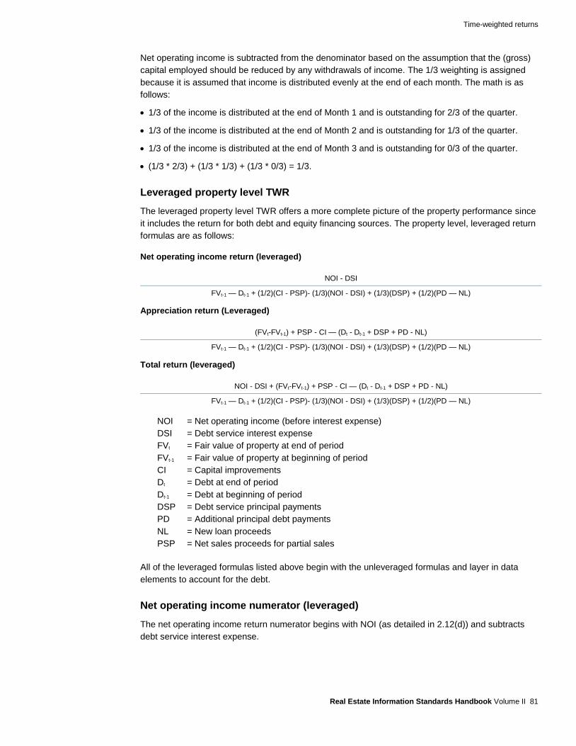
Net operating income is subtracted from the denominator based on the assumption that the (gross)
capital employed should be reduced by any withdrawals of income. The 1/3 weighting is assigned
because it is assumed that income is distributed evenly at the end of each month. The math is as
follows:
1/3 of the income is distributed at the end of Month 1 and is outstanding for 2/3 of the quarter.
1/3 of the income is distributed at the end of Month 2 and is outstanding for 1/3 of the quarter.
1/3 of the income is distributed at the end of Month 3 and is outstanding for 0/3 of the quarter.
(1/3 * 2/3) + (1/3 * 1/3) + (1/3 * 0/3) = 1/3.
Leveraged property level TWR
The leveraged property level TWR offers a more complete picture of the property performance since
it includes the return for both debt and equity financing sources. The property level, leveraged return
formulas are as follows:
Net operating income return (leveraged)
NOI - DSI
FVt-1 — Dt-1 + (1/2)(CI - PSP)- (1/3)(NOI - DSI) + (1/3)(DSP) + (1/2)(PD — NL)
Appreciation return (Leveraged)
(FVt-FVt-1) + PSP - CI — (Dt - Dt-1 + DSP + PD - NL)
FVt-1 — Dt-1 + (1/2)(CI - PSP)- (1/3)(NOI - DSI) + (1/3)(DSP) + (1/2)(PD — NL)
Total return (leveraged)
NOI - DSI + (FVt-FVt-1) + PSP - CI — (Dt - Dt-1 + DSP + PD - NL)
FVt-1 — Dt-1 + (1/2)(CI - PSP)- (1/3)(NOI - DSI) + (1/3)(DSP) + (1/2)(PD — NL)
NOI = Net operating income (before interest expense)
DSI = Debt service interest expense
FVt = Fair value of property at end of period
FVt-1 = Fair value of property at beginning of period
CI = Capital improvements
Dt = Debt at end of period
Dt-1 = Debt at beginning of period
DSP = Debt service principal payments
PD = Additional principal debt payments
NL = New loan proceeds
PSP = Net sales proceeds for partial sales
All of the leveraged formulas listed above begin with the unleveraged formulas and layer in data
elements to account for the debt.
Net operating income numerator (leveraged)
The net operating income return numerator begins with NOI (as detailed in 2.12(d)) and subtracts
debt service interest expense.

Time-weighted returns
Real Estate Information Standards Handbook Volume II 82
Appreciation numerator (leveraged)
The leveraged appreciation formula begins with the real estate appreciation calculation and adds a
debt appreciation calculation to arrive at total appreciation (real estate + debt).
Denominator (leveraged)
The denominator for the leveraged property level TWRs is the property’s weighted average equity
over the quarter. Since property level returns focus on property operations and ignore the use of
working capital, the measure of property value is defined as average real estate value less average
debt value adjusted for cash flow items that affect the real estate and debt.
For the debt items, new debt loan proceeds and additional principal debt payments (i.e. balloon
payments, debt pay-offs and other non-scheduled debt payments) are assumed to occur mid-period
following the same logic employed for capital expenditures and partial sales, so they are weighted at
1/2. New loan proceeds are subtracted because they result in an increase to the beginning debt
value and debt payments are added because they result in a decrease to the beginning balance.
Another way of looking at it is that new loan proceeds result in a cash inflow to the property which is
then distributed and therefore a reduction of equity. Debt payments are funded by contributions and
therefore result in an increase of equity.
Regularly scheduled principal payments are added back at 1/3 based on the assumption that the
principal payments are made evenly at the beginning of each month and the assumed contribution is
received at the end of each month. The math is the same as the 1/3 used for the NOI deduction.
1/3 of the principal is paid at the beginning of Month 1 and is outstanding for 2/3 of the quarter.
1/3 of the principal is paid at the beginning of Month 2 and is outstanding for 1/3 of the quarter.
1/3 of the principal is paid at the end of Month 3 and is outstanding for 0/3 of the quarter.
(1/3 * 2/3) + (1/3 * 1/3) + (1/3 * 0/3) = 1/3.
Investment level TWRs
Investment level TWRs reflect the performance of a single investment or group of investments,
whether that investment is wholly-owned or a joint venture. Investment level TWRs differ from
property level in that the full scope of the investment, including ownership level activity (use of
working capital, owner expenses, etc), is included in the calculation.
Before fee vs. after fee
Investment level returns are generally presented or reported in two forms — before investment
management fees (also known as pre-fee or gross of fees) and after investment management fees
(also known as post-fee or net of fees).
For return purposes, the GIPS® standards only consider advisory fees and incentive fees (including
carried interest paid to the advisor) when distinguishing between the two calculations10
. As such,
fees generally do not include property management fees, construction management fees, acquisition
fees, disposition fees or any other fees that are paid to the investment manager. If, however, these
types of fees are deemed to be over-market and paid in lieu of normal advisory or incentive fees, it is
10
CFA Institute. (2010) Global Investment Performance Standards – Guidance Statement on Fees
www.gipsstandards.org
Time-weighted returns
Real Estate Information Standards Handbook Volume II 83
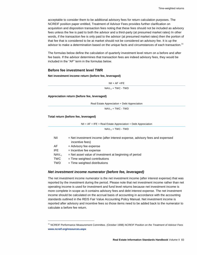
acceptable to consider them to be additional advisory fees for return calculation purposes. The
NCREIF position paper entitled, Treatment of Advisor Fees provides further clarification on
acquisition and disposition transaction fees noting that these fees should not be included as advisory
fees unless the fee is paid to both the advisor and a third-party (at presumed market rates) In other
words, if the transaction fee is only paid to the advisor (at presumed market rates) then the portion of
that fee that is considered to be at market should not be considered an advisory fee. It is up the
advisor to make a determination based on the unique facts and circumstances of each transaction.11
The formulas below define the calculation of quarterly investment level return on a before and after
fee basis. If the advisor determines that transaction fees are indeed advisory fees, they would be
included in the “AF” term in the formulas below.
Before fee investment level TWR
Net investment income return (before fee, leveraged)
NII + AF +IFE
NAVt-1 + TWC - TWD
Appreciation return (before fee, leveraged)
Real Estate Appreciation + Debt Appreciation
NAVt-1 + TWC - TWD
Total return (before fee, leveraged)
NII + AF + IFE + Real Estate Appreciation + Debt Appreciation
NAVt-1 + TWC - TWD
NII = Net investment income (after interest expense, advisory fees and expensed
incentive fees)
AF = Advisory fee expense
IFE = Incentive fee expense
NAVt-1 = Net asset value of investment at beginning of period
TWC = Time weighted contributions
TWD = Time weighted distributions
Net investment income numerator (before fee, leveraged)
The net investment income numerator is the net investment income (after interest expense) that was
reported by the investment during the period. Please note that net investment income rather than net
operating income is used for investment and fund level returns because net investment income is
more complete in scope as it contains advisory fees and debt interest expense. The net investment
income should be calculated on the accrual basis of accounting in accordance with the accounting
standards outlined in the REIS Fair Value Accounting Policy Manual. Net investment income is
reported after advisory and incentive fees so those items need to be added back to the numerator to
calculate a before fee return.
11
NCREIF Performance Measurement Committee. (October 1998) NCREIF Position on the Treatment of Advisor Fees
www.ncreif.org/resources.aspx

Time-weighted returns
Real Estate Information Standards Handbook Volume II 84
Appreciation numerator (before fee, leveraged)
The appreciation numerator measures the change (increase or decrease) in investment value not
caused by capital improvements, sales, or refinancing. Real estate and debt should be reported in
accordance with the accounting standards outlined in the REIS standards and valuations should be
completed on a quarterly basis in accordance with the valuation standards outlined in the REIS
standards. Appreciation included in the leveraged numerator should include both realized and
unrealized real estate and debt appreciation (if applicable).
Denominator (before fee, leveraged)
The denominator for the investment level TWR is the weighted average equity of the investment
over the quarter. Weighted average equity is calculated by adjusting the beginning of quarter net
asset value for equity transactions (contributions and distributions) that occur during the quarter.
Each contribution or distribution that occurs during the period needs to be time weighted by
multiplying it by a time weighting factor based on the date of the transaction. For return purposes,
contributions include original contributions as well as reinvestments of capital and distributions
include both operating and return of capital distributions. The initial contribution for the investment is
not weighted (or it can be thought of as weighted at 100%). The denominator is the actual number of
days that the investment was active during the period. Usually, the denominator will equal the total
number of days in the quarter, however if the transaction is either the very first or last transaction for
the investment, then the denominator is adjusted to match the number of days the investment was
active for the period. The numerator is the total number of days remaining in the period after the
equity transaction occurs.
For contributions: Contributions in the current quarter are weighted based upon the number of
days the contribution was in the fund during the quarter commencing with the day the contribution
was received.
For example: Beginning Net Asset Value for 2Q 2008 $10,000,000
Contribution of $5,000,000 on 5/30/2008
Calculation: 5,000,000*(32/91) = $1,758,241.76
Beginning NAV + Weighted Contribution = Denominator
$10,000,000 + $1,758,241.76 = $11,758,241.76
For distributions: Distributions in the current quarter are weighted based upon the number of days
the distribution/withdrawal was out of the fund during the quarter commencing with the day following
the date distribution/withdrawal was paid.
For example: Beginning Net Asset Value for 2Q 2008 $10,000,000
Distribution of $5,000,000 on 5/30/2008
Calculation: 5,000,000*(31/91) = $1,703,296.70
Beginning NAV - Weighted Distribution = Denominator
$10,000,000 - $1,703,296.70 = $8,296,703.30

Time-weighted returns
Real Estate Information Standards Handbook Volume II 85
Note: Another factor that impacts weighted average equity is cash redemptions/withdrawals by
investors, which are not cash distributions but rather an investor’s removal of all or part of its equity
from the fund. Such equity transactions are weighted in a manner identical to the weighting of cash
distributions described above.
After fee investment level TWR
Net investment income return (after fee, leveraged)
NII
NAVt-1 + TWC - TWD
Appreciation return (after fee, leveraged)
Real Estate Appreciation + Debt Appreciation - IFC
NAVt-1 + TWC - TWD
Total return (after fee, leveraged)
NII + Real Estate Appreciation + Debt Appreciation - IFC
NAVt-1 + TWC - TWD
NII = Net investment income (after interest expense, advisory fees and expensed
incentive fees)
IFC = Change in capitalized incentive fee
NAVt-1 = Net asset value of investment at beginning of period
TWC = Time weighted contributions
TWD = Time weighted distributions
The investment management fees consist of the quarterly investment management fee that is
charged by an advisor as well as any incentive fees earned by the advisor (and therefore do not
include any fees paid to the General Partner including developer promotes). Other fees charged by
the investment advisor, including property management fees, financing fees and development fees
are typically not included as a fee when calculating an after fee return. In other words, the spread
between before and after fee return does not include these items. Transaction fees including
acquisition and disposition are explained above.
Before and after fee investment level TWR denominators are the same because there is only one
weighted average equity for the period. The contributions and distributions used in the denominators
are always after fee and are not adjusted to be before fee even when calculating a before fee return.
Net investment income numerator (after fee, leveraged)
The after fee investment level net investment income numerator is the net investment income (after
interest expense) that was reported by the investment during the period. Net investment income is
already reported after advisory and incentive fees on the income statement, so no adjustment needs
to be made for these items when calculating an after fee return.
Appreciation numerator (after fee, leveraged)
The after fee investment level appreciation numerator subtracts any change in capitalized incentive
fee that was accrued during the quarter. Generally, incentive fees that are earned based on changes
in an investment’s fair value are recorded as unrealized appreciation and impact the appreciation
Time-weighted returns
Real Estate Information Standards Handbook Volume II 86
return, and fees that result from meeting and exceeding operating result goals are expensed and
impact the net investment income return.
Fund level TWR’s
A fund level TWR (also referred to as account or portfolio level) is the aggregation of all of the
investments made by the entity and the amounts earned or incurred which relate to the entity but are
not specifically attributable to a particular investment Similar to investment level returns, the fund
level TWRs are very broad in nature and try to capture all activity, which includes, but is not limited
to, those revenues and expenses applicable to the fund, taken as a whole, such as audit and
appraisal fees, interest income and portfolio borrowings. In essence, this return measures the
performance of the manager in terms of how well the management team performed its specified
strategy.
Before fee vs. after fee
The REIS standards require quarterly reporting of fund level total and component TWR before and
after fees for all Funds. The formulas below define the calculation of quarterly fund level returns on a
before and after fee basis.
For return purposes, the GIPS® standards only consider advisory fees and incentive fees (including
carried interest paid to the advisor) when distinguishing between the two calculations12
. As such,
fees generally do not include property management fees, construction management fees, acquisition
fees, disposition fees or any other fees that are paid to the investment manager. If, however, these
types of fees are deemed to be over-market and paid in lieu of normal advisory or incentive fees, it is
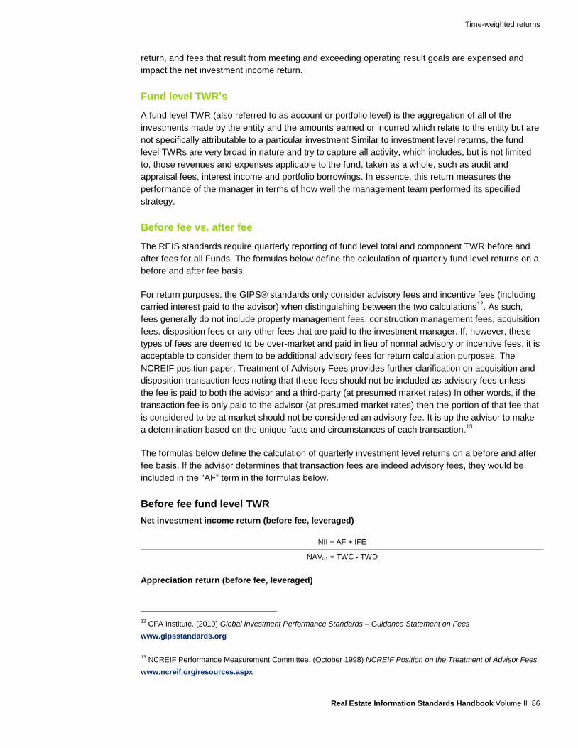
acceptable to consider them to be additional advisory fees for return calculation purposes. The
NCREIF position paper, Treatment of Advisory Fees provides further clarification on acquisition and
disposition transaction fees noting that these fees should not be included as advisory fees unless
the fee is paid to both the advisor and a third-party (at presumed market rates) In other words, if the
transaction fee is only paid to the advisor (at presumed market rates) then the portion of that fee that
is considered to be at market should not be considered an advisory fee. It is up the advisor to make
a determination based on the unique facts and circumstances of each transaction.13
The formulas below define the calculation of quarterly investment level returns on a before and after
fee basis. If the advisor determines that transaction fees are indeed advisory fees, they would be
included in the “AF” term in the formulas below.
Before fee fund level TWR
Net investment income return (before fee, leveraged)
NII + AF + IFE
NAVt-1 + TWC - TWD
Appreciation return (before fee, leveraged)
12
CFA Institute. (2010) Global Investment Performance Standards – Guidance Statement on Fees
www.gipsstandards.org
13 NCREIF Performance Measurement Committee. (October 1998) NCREIF Position on the Treatment of Advisor Fees
www.ncreif.org/resources.aspx
Time-weighted returns
Real Estate Information Standards Handbook Volume II 87
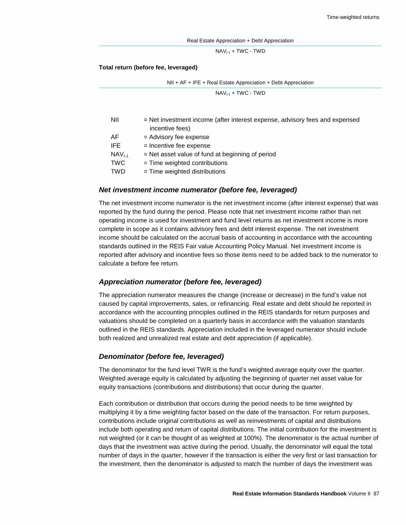
Real Estate Appreciation + Debt Appreciation
NAVt-1 + TWC - TWD
Total return (before fee, leveraged)
NII + AF + IFE + Real Estate Appreciation + Debt Appreciation
NAVt-1 + TWC - TWD
NII = Net investment income (after interest expense, advisory fees and expensed
incentive fees)
AF = Advisory fee expense
IFE = Incentive fee expense
NAVt-1 = Net asset value of fund at beginning of period
TWC = Time weighted contributions
TWD = Time weighted distributions
Net investment income numerator (before fee, leveraged)
The net investment income numerator is the net investment income (after interest expense) that was
reported by the fund during the period. Please note that net investment income rather than net
operating income is used for investment and fund level returns as net investment income is more
complete in scope as it contains advisory fees and debt interest expense. The net investment
income should be calculated on the accrual basis of accounting in accordance with the accounting
standards outlined in the REIS Fair value Accounting Policy Manual. Net investment income is
reported after advisory and incentive fees so those items need to be added back to the numerator to
calculate a before fee return.
Appreciation numerator (before fee, leveraged)
The appreciation numerator measures the change (increase or decrease) in the fund’s value not
caused by capital improvements, sales, or refinancing. Real estate and debt should be reported in
accordance with the accounting principles outlined in the REIS standards for return purposes and
valuations should be completed on a quarterly basis in accordance with the valuation standards
outlined in the REIS standards. Appreciation included in the leveraged numerator should include
both realized and unrealized real estate and debt appreciation (if applicable).
Denominator (before fee, leveraged)
The denominator for the fund level TWR is the fund’s weighted average equity over the quarter.
Weighted average equity is calculated by adjusting the beginning of quarter net asset value for
equity transactions (contributions and distributions) that occur during the quarter.
Each contribution or distribution that occurs during the period needs to be time weighted by
multiplying it by a time weighting factor based on the date of the transaction. For return purposes,
contributions include original contributions as well as reinvestments of capital and distributions
include both operating and return of capital distributions. The initial contribution for the investment is
not weighted (or it can be thought of as weighted at 100%). The denominator is the actual number of
days that the investment was active during the period. Usually, the denominator will equal the total
number of days in the quarter, however if the transaction is either the very first or last transaction for
the investment, then the denominator is adjusted to match the number of days the investment was

Time-weighted returns
Real Estate Information Standards Handbook Volume II 88
active for the period. The numerator is the total number of days remaining in the period after the
equity transaction occurs.
For contributions: Contributions in the current quarter are weighted based upon the number of
days the contribution was in the fund during the quarter commencing with the day the contribution
was received.
For example: Beginning Net Asset Value for 2Q 2008 $10,000,000
Contribution of $5,000,000 on 5/30/2008
Calculation: 5,000,000*(32/91) = $1,758,241.76
Beginning NAV + Weighted Contribution = Denominator
$10,000,000 + $1,758,241.76 = $11,758,241.76
For distributions: Distributions in the current quarter are weighted based upon the number of days
the distribution/withdrawal was out of the fund during the quarter commencing with the day following
the date distribution/withdrawal was paid.
For example: Beginning Net Asset Value for 2Q 2008 $10,000,000
Distribution of $5,000,000 on 5/30/2008
Calculation: 5,000,000*(31/91) = $1,703,296.70
Beginning NAV - Weighted Distribution = Denominator
$10,000,000 - $1,703,296.70 = $8,296,703.30
Note: Another factor that impacts weighted average equity is cash redemptions/withdrawals by
investors, which are not cash distributions but rather an investor’s removal of all or part of its equity
from the fund. Such equity transactions are weighted in a manner identical to the weighting of cash
distributions described above.
After fee fund level TWR
Net investment income return (after fee, leveraged)
NII
NAVt-1 + TWC - TWD
Appreciation return (after fee, leveraged)
Real Estate Appreciation + Debt Appreciation — IFC
NAVt-1 + TWC - TWD
Total return (after fee, leveraged)
NII + Real Estate Appreciation + Debt Appreciation - IFC
NAVt-1 + TWC - TWD
NII= Net investment income (after interest expense, advisory fees and expensed
incentive fees)

Time-weighted returns
Real Estate Information Standards Handbook Volume II 89
IFC = Change in capitalized incentive fee
NAVt-1 = Net asset value of investment at beginning of period
TWC = Time weighted contributions
TWD = Time weighted distributions
The investment management fees consist of the quarterly investment management fee that is
charged by an advisor as well as any incentive fees (and therefore do not include any fees paid to
the General Partner including developer promotes). Other fees earned by the investment advisor,
including property management fees, financing fees and development fees are typically not layered
in when calculating an after fee return. In other words, the spread between before and after fee
returns does not include these items. Transaction fees including acquisition and disposition are
explained above.
Before and after fee fund level TWR denominators are the same because there is only one weighted
average equity for the period. The contributions and distributions used in the denominators are
always after fee and are not adjusted to be before fee even when calculating a before fee return.
Income numerator (after fee, leveraged)
The after fee fund level net investment income numerator is the net investment income (after interest
expense) that was reported by the investment during the period. Net investment income is already
reported after advisory and inventive fees on the income statement, so no adjustment needs to be
made for these items when calculating an after fee return.
Appreciation numerator (after fee, leveraged)
The after fee investment level appreciation numerator subtracts any change in capitalized incentive
fee that was accrued during the quarter. Generally, incentive fees that are earned based on changes
in an investment’s fair value are recorded as unrealized appreciation and impact the appreciation
return, and fees that result from meeting and exceeding operating result goals are expensed and
impact the net investment income return.

Money-weighted returns (IRRs)
Real Estate Information Standards Handbook Volume II 90
Money-weighted returns (IRRs)
Definition
The internal rate of return (IRR) is the annualized implied discount rate (effective compounded
nominal rate) that equates the present value of all of the appropriate cash inflows associated with an
investment with the sum of the present value of all the appropriate cash outflows accruing from it
and the present value of the unrealized residual portfolio. IRRs are commonly used in the
investment industry to measure the performance of the investment (contrasted with TWRs which are
used to measure the performance of the investment manager). The IRR is also known as:
A “money-weighted” return because, unlike a TWR, the entity’s cash flows do impact the IRR
formula.
The rate of return that results in a net present value of zero.
Sample IRR Formula
The IRR formula discounts flows F1 through Fn back to F0 where: F0 is the original investment; and
F1 through Fn are the cash flows for each applicable period. Typically F1 is the net of management
fees. However, it may be the case the firm wishes to calculate a gross IRR, in which case F1 would
be gross management fees. If the entity has not yet been liquidated, the ending cash flow, Fn, will
consist of the latest period’s operating cash flows plus an estimate of the net residual value.
F0 + F1 + F2 + F3 + .. + Fn = 0
1+IRR (1+IRR)2 (1+IRR)
3 (1+IRR)
n
As used herein, period refers to the date of the cash inflows and outflows. For accounts which are compliant with the REIS standards, the minimum period is quarterly.
Solution by financial calculator
Numerical iterations can easily become cumbersome and inefficient. Therefore, using a financial
calculator can simplify this process. Microsoft Excel contains two functions that can be used for this
calculation: the IRR function (“=IRR”) and the XIRR function (“=XIRR”). Both functions produce an
IRR result however they use slightly different calculation methodologies and assumptions so the
user needs to determine which function to use to best meet its needs. Below is a comparison of
these functions:
Excel IRR function
User inputs a series of cash flows which are assumed to occur at equal intervals.
If a period’s cash flow is zero, you must enter a zero, as a blank will result in a wrong answer.
Does not annualize the result.
Money-weighted returns (IRRs)
Real Estate Information Standards Handbook Volume II 91
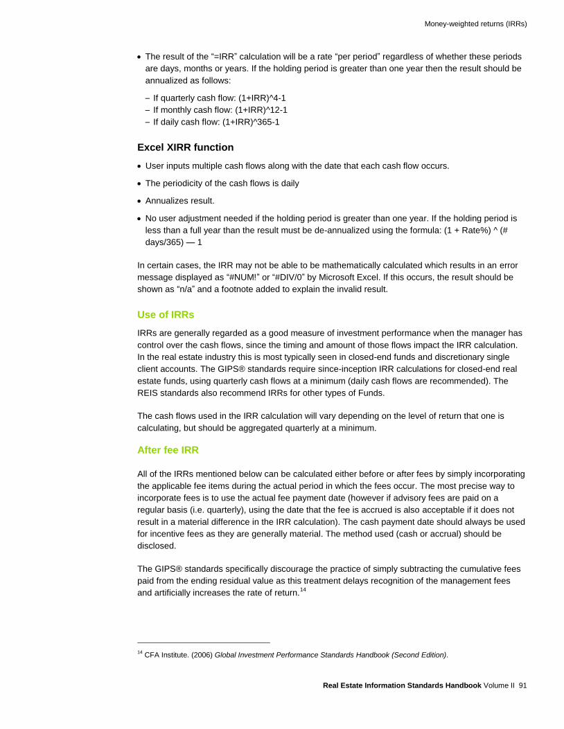
The result of the “=IRR” calculation will be a rate “per period” regardless of whether these periods
are days, months or years. If the holding period is greater than one year then the result should be
annualized as follows:
– If quarterly cash flow: (1+IRR)^4-1
– If monthly cash flow: (1+IRR)^12-1
– If daily cash flow: (1+IRR)^365-1
Excel XIRR function
User inputs multiple cash flows along with the date that each cash flow occurs.
The periodicity of the cash flows is daily
Annualizes result.
No user adjustment needed if the holding period is greater than one year. If the holding period is
less than a full year than the result must be de-annualized using the formula: (1 + Rate%) ^ (#
days/365) — 1
In certain cases, the IRR may not be able to be mathematically calculated which results in an error
message displayed as “#NUM!” or “#DIV/0” by Microsoft Excel. If this occurs, the result should be
shown as “n/a” and a footnote added to explain the invalid result.
Use of IRRs
IRRs are generally regarded as a good measure of investment performance when the manager has
control over the cash flows, since the timing and amount of those flows impact the IRR calculation.
In the real estate industry this is most typically seen in closed-end funds and discretionary single
client accounts. The GIPS® standards require since-inception IRR calculations for closed-end real
estate funds, using quarterly cash flows at a minimum (daily cash flows are recommended). The
REIS standards also recommend IRRs for other types of Funds.
The cash flows used in the IRR calculation will vary depending on the level of return that one is
calculating, but should be aggregated quarterly at a minimum.
After fee IRR
All of the IRRs mentioned below can be calculated either before or after fees by simply incorporating
the applicable fee items during the actual period in which the fees occur. The most precise way to
incorporate fees is to use the actual fee payment date (however if advisory fees are paid on a
regular basis (i.e. quarterly), using the date that the fee is accrued is also acceptable if it does not
result in a material difference in the IRR calculation). The cash payment date should always be used
for incentive fees as they are generally material. The method used (cash or accrual) should be
disclosed.
The GIPS® standards specifically discourage the practice of simply subtracting the cumulative fees
paid from the ending residual value as this treatment delays recognition of the management fees
and artificially increases the rate of return.14
14
CFA Institute. (2006) Global Investment Performance Standards Handbook (Second Edition).

Money-weighted returns (IRRs)
Real Estate Information Standards Handbook Volume II 92
Often times, a closed-end fund will use a credit facility to fund initial operations thus delaying the first
capital cash flow. To the extent that those initial operations include the payment of fees, the since
inception fees would be incorporated as negative cash flows on the date of the initial cash flow.
Property level IRRs
At the property level, the inputs for the IRR formula are based on property cash flows, which serve
as surrogates to the actual cash flows between the property and investors.
In general, the IRR calculation should start with the initial cash flow on the property’s acquisition
date and end with the final cash flow on the property’s disposition date. If the property has not yet
been liquidated, the ending cash flow, will consist of the latest period’s operating cash flows plus an
estimate of the net residual value (fair value of real estate less estimated costs to sell less fair value
of debt).
Unleveraged property level IRR
The initial cash flow for the unleveraged IRR calculation is the total amount that is paid for the
acquisition (before debt) which should include the property’s purchase price plus acquisition costs.
Other cash flows over the life of the property include the property’s quarterly net operating income
(before interest expense) less capital improvements. Net operating income is depicted as a positive
cash flow while net operating loss and capital improvements are shown as negative cash flows in
the calculation.
The ending cash flow is the property’s final real estate sale proceeds (before debt payoff), if property
has been sold. If the property has not yet been liquidated, the ending cash flow, will consist of the
latest period’s operating cash flows plus an estimate of the residual real estate value (fair value of
real estate less estimated costs to sell).
Leveraged property level IRR
The initial cash flow is the property’s purchase price, less initial debt balance.
Other cash flows over the life of the property include the property’s net operating income less capital
improvements less debt service payments (principal and interest). Net income is depicted as a
positive cash flow while net loss, capital improvements, and debt service payments (principal and
interest) are shown as negative cash flows in the calculation. In addition, new debt placed on a
property after acquisition is treated as a positive cash flow in the calculation.
The ending cash flow is the property’s final real estate sale proceeds after debt payoff amount, if
property has been sold. If the property has not yet been liquidated, the ending cash flow, will consist
of the latest period’s operating cash flows plus an estimate of the net residual value (fair value of
real estate less estimated costs to sell less fair value of debt).
Investment level IRRs
At the investment level, the inputs for the IRR formula are based on the actual cash flows between
the investor and the investment. The IRR for each individual investor may actually be different if the
investor’s transactions occur on different dates.
In general, the IRR calculation for each investor should start with the initial cash flow on the date of
the investor’s first capital contribution and end with the final cash flow on the date that the investor
Money-weighted returns (IRRs)
Real Estate Information Standards Handbook Volume II 93
received his final distribution. If the investment has not yet been liquidated, the ending cash flow will
consist of the latest period’s operating cash flows plus the investments net asset value less
estimated sale costs at the IRR calculation date.
Investment level IRRs are typically only shown on a leveraged basis because the leveraged amount
represents the return that the investor is actually realizing and it is difficult to strip leverage out of
actual contributions and distributions.
Leveraged investment level IRR
The initial cash flow is the investor’s first contribution.
Other cash flows over the life of the investment include actual contributions (including
reinvestments) and distributions (both operating and return of capital) between the investor and the
investment. Contributions are shown as negative cash flows and distributions are positive cash flows
in the calculation.
The ending cash flow is the investor’s final liquidating distribution, if the investment has been
liquidated. If the investment has not yet been liquidated, the ending cash flow will consist of the
latest period’s operating cash flows plus the investments net asset value less estimated sale costs at
the IRR calculation date.
Fund level IRRs
At the fund level, the inputs for the IRR formula are based on the actual cash flows between the
investors and the fund. General partner cash flows are not included in this calculation. Where an
affiliate of the general partner is created for co-investment purposes, the affiliate entity would be
included in the calculation as long as the entity is treated the same as other limited partners.
In general, the IRR calculation should start with the initial cash flow on the date of the first capital
contribution and end with the final cash flow on the date that of the final liquidating distribution. If the
investment has not yet been liquidated, the ending cash flow will consist of the latest period’s
operating cash flows plus the investments net asset value less estimated sale costs at the IRR
calculation date.
Fund level IRRs are typically only shown on a leveraged basis because the leveraged amount
represents the return that the investor is actually realizing and it is difficult to strip leverage out of
actual contributions and distributions.
Leveraged fund level IRR
The initial cash flow is the first investor’s contribution.
Other cash flows over the life of the fund include actual contributions and distributions (both
operating and return of capital) between the investors and the fund. Contributions are shown as
negative cash flows and distributions are positive cash flows in the calculation.
The ending cash flow is the final liquidating distribution made to the investors, if the fund has been
liquidated. If the investment has not yet been liquidated, the ending cash flow will consist of the
latest period’s operating cash flows plus the investments net asset value less estimated sale costs at
the IRR calculation date.

Equity multiples
Real Estate Information Standards Handbook Volume II 94
Equity multiples
Definition
In general terms, an equity multiple is a performance metric that measures a certain aspect of an
entity’s financial performance. Multiples are shown as ratios, with one financial input in the
numerator and another in the denominator, both of which are typically presented for the entire life of
the investment rather some discrete time period (month, quarter, etc).
Use of multiples
Used in conjunction with time-weighted returns and IRRs, multiples provide greater transparency
when analyzing performance. The four commonly used multiples required for closed-end real estate
funds in the GIPS® standards are presented below. Although multiples are not a current
requirement in the GIPS® standards for all real estate vehicles, GIPS® does recommend presenting
multiples as useful information for prospective and existing clients. The GIPS® standards require
disclosing these multiples on closed-end real estate funds on an annual basis.
Note on fees
Multiples listed below are presumed to be shown after all fees, including acquisition, asset
management, disposition, incentive fees and carried interest/promotes. Fees paid outside of the
fund should also be taken into consideration for these calculations. In order to estimate before fee
multiples, the ratios would need to be adjusted. Distributions would be increased for cumulative fees,
and capital contributions would be reduced for fees contributed. Residual values would also be
adjusted for any fee accruals or allocations.
Investment multiple or total value to paid-in capital multiple (TVPI)
This investment multiple gives users information regarding the value of the investment relative to its
cost basis, not taking into consideration the time invested. As an example, a multiple equal to 1.50 is
typically read as the investors have $1.50 of value in the fund for every $1 invested.
TV
PIC
TV = Total value
Fund: Sum of residual fund net assets (NAV) plus aggregate fund distributions
Investment: Sum of residual investment net assets (NAV) plus aggregate distributions
Property: Sum of property fair value (net of debt) plus aggregate distributions paid since
inception (note: if actual property distributions are not separately maintained,
estimates can be calculated by aggregating the property’s net operating income
(after interest expense) and subtracting principal).
PIC = Paid In capital
Fund: Cumulative capital contributed to the fund

Equity multiples
Real Estate Information Standards Handbook Volume II 95
Investment: Cumulative capital contributed to the investment
Property: Cumulative capital contributed to the property (note: if actual property contributions
are not separately maintained, estimates can be calculated by aggregating cash
paid at acquisition plus capital additions)
Realization multiple or cumulative distributions to paid-in capital multiple (DPI)
The DPI measures what portion of the return has actually been returned to the investors. The DPI
will be zero until distributions are made. As the fund matures, typically the DPI will increase. When
the DPI is the equivalent of one, the fund has broken even. Consequently, a DPI of greater than one
suggests the fund has generated profit to the investors.
D
PIC
D = Total distributions
Fund: Aggregate fund distributions paid since inception
Investment: Aggregate investment distributions paid since inception
Property: Aggregate property distributions paid since inception (note: if actual property
distributions are not separately maintained, estimates can be calculated by
aggregating the property’s net operating income (after interest expense) and
subtracting principal payments).
PIC = Paid in capital
Fund: Cumulative capital contributed to the fund
Investment: Cumulative capital contributed to the investment
Property: Cumulative capital contributed to the property (note: if actual property contributions
are not separately maintained, estimates can be calculated by aggregating cash
paid at acquisition plus capital additions)
Paid-in capital multiple or paid-in capital to committed capital multiple (PIC)
This ratio gives information regarding how much of the total commitments have been drawn down.
The paid in capital is the cumulative drawdown amount, or the aggregate amount of committed
capital actually transferred to a fund or property. Typically a number such as .80 is read as 80% of
the fund’s capital commitments have been drawn from investors.
PIC
CC
PIC = Paid in capital
Fund: Cumulative capital contributed to the fund
Investment: Cumulative capital contributed to the investment
Property: Cumulative capital contributed to the property (note: if actual property contributions
are not separately maintained, estimates can be calculated by aggregating cash
paid at acquisition plus capital additions)
CC = Committed capital
Fund: Cumulative fund PIC plus unfunded capital

Equity multiples
Real Estate Information Standards Handbook Volume II 96
Investment: Cumulative investment PIC plus unfunded capital
Property: Cumulative property PIC plus unfunded commitments (e.g. renovation reserves)
Residual multiple or residual value to paid-in capital multiple (RVPI)
This ratio provides a measure of how much of the return is unrealized. As the fund matures, the
RVPI will increase to a peak and then decrease as the fund eventually liquidates to a residual fair
value of zero. At that point, the entire return of the fund has been distributed.
Residual value is defined as remaining equity in fund or property. An RVPI of .70 would indicate an
amount equal to 70% of the fund’s paid-in capital remains unrealized.
RV
PIC
RV = Residual value
Fund: Net asset value (NAV) of the fund
Investment: Net asset value (NAV) of the investment
Property: Property fair value net of debt
PIC = Paid in capital
Fund: Cumulative capital contributed to the fund
Investment: Cumulative capital contributed to the investment
Property: Cash Cumulative capital contributed to the property (note: if actual property
contributions are not separately maintained, estimates can be calculated by
aggregating cash paid at acquisition plus capital additions)
Other performance metrics
Real Estate Information Standards Handbook Volume II 97
Other performance metrics
Introduction
Within our industry, the time-weighted return (TWR) and money-weighted return (IRR) are far and
away the most frequently calculated performance metrics used to report manager and investment
performance. However, other metrics are available and investors, consultants and managers are
finding them increasingly helpful to supplement these traditional measures. This section will explore
some of these alternative metrics and provide guidance into their use and calculation.
The alternative metrics which will be discussed can be broadly categorized as follows;
Alternative component return calculations
Leverage ratios
Measures of dispersion
Risk measures
Please note that all of the metrics that are described below are expected to be used in conjunction
with the traditional TWRs and IRRs as supplemental information, and not meant to be a
replacements for those measures.
Alternative Compenent Return Calculations
In this section, three different types of component calculations which are meant to be alternatatives
to the traditional income and appreciation splits that are commonly used in our industry are
described. One of the criticisms of the traditional accrual-based income TWR is that it does not
provide enough information about the cash that is actually generated, so these metrics attempt to
provide that missing detail. All three of these alternatives are similar in that they provide the user
with a sense of how the cash flow and/or distributions of the investment are impacting total returns.
Distribution and price change returns- Investment/ Fund Level
TWR indexes that are used in most asset classes outside of institutional private real estate break the
total time. The component returns used in our industry have always been slightly different from the
concepts listed abovie. Instead of a Distribution Return, we calculate an income return which is
based on accrual basis net income earned, not cash that is actually distributed. In addition, our
appreciation return is based on value change net of capital expenditures, rather than the pure
market price change concept that is foundin the Price Change Return.
The income and appreciation definitions that we have traditionally used serve us well and make
sense conceptually when applied to a property level calculation. The split gives the user important

Other performance metrics
Real Estate Information Standards Handbook Volume II 98
information on the component of the return that the owner/adviser has less control over
(appreciation) versus the part which can be more actively managed (income). For investment level
returns however, the income and appreciation components may be less theoretically supported and
there are some that would argue that the Distribution and Price Change Return components that are
used prevalently in other asset classes may be more appropriate or at the very least can provide
useful supplemental information.
Distribution return- Investment/ Fund Level
The Distribution Return shows the amount of actual cash that is distributed to investors as a portion
of weighted average equity for any given quarter. The return is meant to provide investors with a true
cash basis performance measure which supplements what is currently lacking in the existing income
and total return measures. This return is thought to be more comparable to the income return and/or
divided yield that is reported in other asset classes than the existing income return is. The formula is
as follows:
Distribution return formula
LP Distributions Net of Fees
LP Weighted Average Equity
The distribution of net fees in the formula above is defined as a distribution to the limited partners
that is pro-rata to the whole class of investors (excludes redemptions). This includes any
distributions that are reinvested. Distributions should include the limited partner level distributions
and ownership share only. Fees that are actually paid in the current period should be deducted from
distributions whether those fees are withheld from the actual distributions or paid via an investor
contribution.
Weighted average equity is defined in 5.01(d) above.
Price change return
The Price Change Return is meant to measure the change in NAV that is not attributable to investor
equity transactions (contributions, distributions or redemptions) as a portion of weighted average
equity for any given quarter. The formula is as follows:
Price change return formula
LP NAV1 ex distribution — LP NAV
0 ex previous quarter distribution + LP redemptions — LP Contributions
LP Weighted Average Equity
The LP NAV (Net Asset Value) in the formula above is defined as all LP assets less all liabilities
reflected on a market value basis. It is assumed that these amounts should be taken directly from
the investments audited financial statements which are reported on a fair market value basis of
accounting in accordance with the REIS standards.
Redemptions are defined as a distribution that is not pro-rata to the whole class of investors.
Weighted average equity is defined in 5.01(d) above.

Other performance metrics
Real Estate Information Standards Handbook Volume II 99
Cash Flow and Price Change Returns – Property Level
The Cash Flow and Price Change Return are very similar to the Distribution and Price Change
Return that were discussed above except that these alternative return measures are meant to be
applied using property level inputs rather than investment or fund level data. Both of these metrics
can currently be calculated using the NCREIF query tool.
Cash Flow Return – Property Level
The Cash Flow Return shows the approximate amount of cash from a property that is assumed to
be distributed to investors as a portion of weighted average equity for any given quarter. We say
that the cash is “assumed” to be distributed because at the property level we are using property level
cash flow (net operating income less capital improvements) as a surrogate for actual distributions
since actual distributions are not tracked as part of the property level TWR formula. This return is
meant to provide investors with an estimate of cash basis performance which supplements what is
currently lacking in the existing property level income and total return measures. The cash flow
return is comparable to the dividend yield that is reported in other asset classes.
To calculate the cash flow return, the user needs to only make a very simple change
to the existing property level income return formula. Current quarter capital
improvements should be subtracted from the income return numerator instead of the
appreciation return numerator, resulting in a cash flow return (and conversely the
appreciation return will become a price change return). The unleveraged formula is
as follows: NOI – CI
FVt-1 + (1/2)(CI - PSP)- (1/3)(NOI)
NOI = Net operating income (before interest expense)
FVt-1 = Fair value of property at beginning of period
CI = Capital improvements
PSP = Net sales proceeds for partial sales
Price Change Return – (Property Level)
The Price Change Return is meant to measure the change in NAV that is not attributable to investor equity transactions (contributions, distributions or redemptions) as a portion of weighted average equity for any given quarter. The formula is as follows:
(FVt-FVt-1) + PSP
FVt-1 + (1/2)(CI - PSP)- (1/3)(NOI)
NOI = Net operating income (before interest expense)
FVt = Fair value of property at end of period
FVt-1= Fair value of property at beginning of period

Other performance metrics
Real Estate Information Standards Handbook Volume II 100
CI = Capital improvements
PSP = Net sales proceeds for partial sales
For more information on the Cash Flow and Price change returns, please refer to the academic
articles that were authored by Young, Geltner, McIntosh and Poutasse in 1995 and 1996.15
Disaggregated income returns
Distributed and retained income returns refer to the division of time-weighted income returns into two
separate components. The dividend policy of the fund should be considered when calculating and
interpreting the results of the return metrics below as each can be materially impacted. Please note
that the aggregate dollar amount of distributed income plus retained income will equal total income.
Distributed income return
Distributed income is defined as the amount of investment income derived from operations that is 1)
actually distributed to investors or 2) credited to investors in the case of investment fund dividend or
income reinvestment programs that are elected by the investor. (Mandatory reinvestment programs
or automatic cash retention programs are not considered elective by the investor). Distributed
income does not include the return of capital or principal, the distribution of realized gains from asset
sales (capital gains) nor proceeds from financing activities. The objective is to present the actual
cash distributions that are derived from customary and ongoing investment management operations
without the distortions related to disposition and refinancing activities.
The distributed income formula is defined below:
Distributed Income
Weighted Average Equity
Weighted average equity is defined in the Time-Weighted Return Section of the Manual.
Retained income return
Retained income portion of the income return is considered materially different (in economic terms)
from the distributed income portion. Retained income simply refers to the income that is earned by
the entity that is not distributed. Retained income can be used in various strategic ways to manage
the real estate portfolio, including but not limited to, debt repayment, acquisition of assets and capital
expenditures on existing assets.
15
M. Young, D. Geltner, W. McIntosh, and D. Poutasse “Defining Commercial Property Income and Appreciation
Returns for Comparability to Stock Marked-Based Measures” Real Estate Finance Vol. 12, No. 2, Summer 1995,pp.
19-30
M. Young, D. Geltner, W. McIntosh, and D. Poutasse “Understanding Equity Real Estate Performance: Insights from
the NCREIF Property Index” Real Estate Review Vol. 25, No. 4, Winter 1996, pp. 4-16
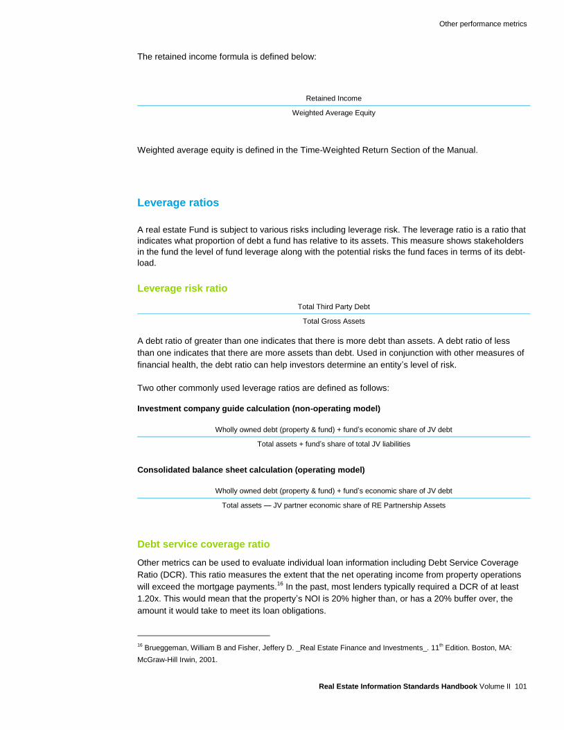
Other performance metrics
Real Estate Information Standards Handbook Volume II 101
The retained income formula is defined below:
Retained Income
Weighted Average Equity
Weighted average equity is defined in the Time-Weighted Return Section of the Manual.
Leverage ratios
A real estate Fund is subject to various risks including leverage risk. The leverage ratio is a ratio that
indicates what proportion of debt a fund has relative to its assets. This measure shows stakeholders
in the fund the level of fund leverage along with the potential risks the fund faces in terms of its debt-
load.
Leverage risk ratio
Total Third Party Debt
Total Gross Assets
A debt ratio of greater than one indicates that there is more debt than assets. A debt ratio of less
than one indicates that there are more assets than debt. Used in conjunction with other measures of
financial health, the debt ratio can help investors determine an entity’s level of risk.
Two other commonly used leverage ratios are defined as follows:
Investment company guide calculation (non-operating model)
Wholly owned debt (property & fund) + fund’s economic share of JV debt
Total assets + fund’s share of total JV liabilities
Consolidated balance sheet calculation (operating model)
Wholly owned debt (property & fund) + fund’s economic share of JV debt
Total assets — JV partner economic share of RE Partnership Assets
Debt service coverage ratio
Other metrics can be used to evaluate individual loan information including Debt Service Coverage
Ratio (DCR). This ratio measures the extent that the net operating income from property operations
will exceed the mortgage payments.16
In the past, most lenders typically required a DCR of at least
1.20x. This would mean that the property’s NOI is 20% higher than, or has a 20% buffer over, the
amount it would take to meet its loan obligations.
16
Brueggeman, William B and Fisher, Jeffery D. _Real Estate Finance and Investments_. 11th Edition. Boston, MA:
McGraw-Hill Irwin, 2001.
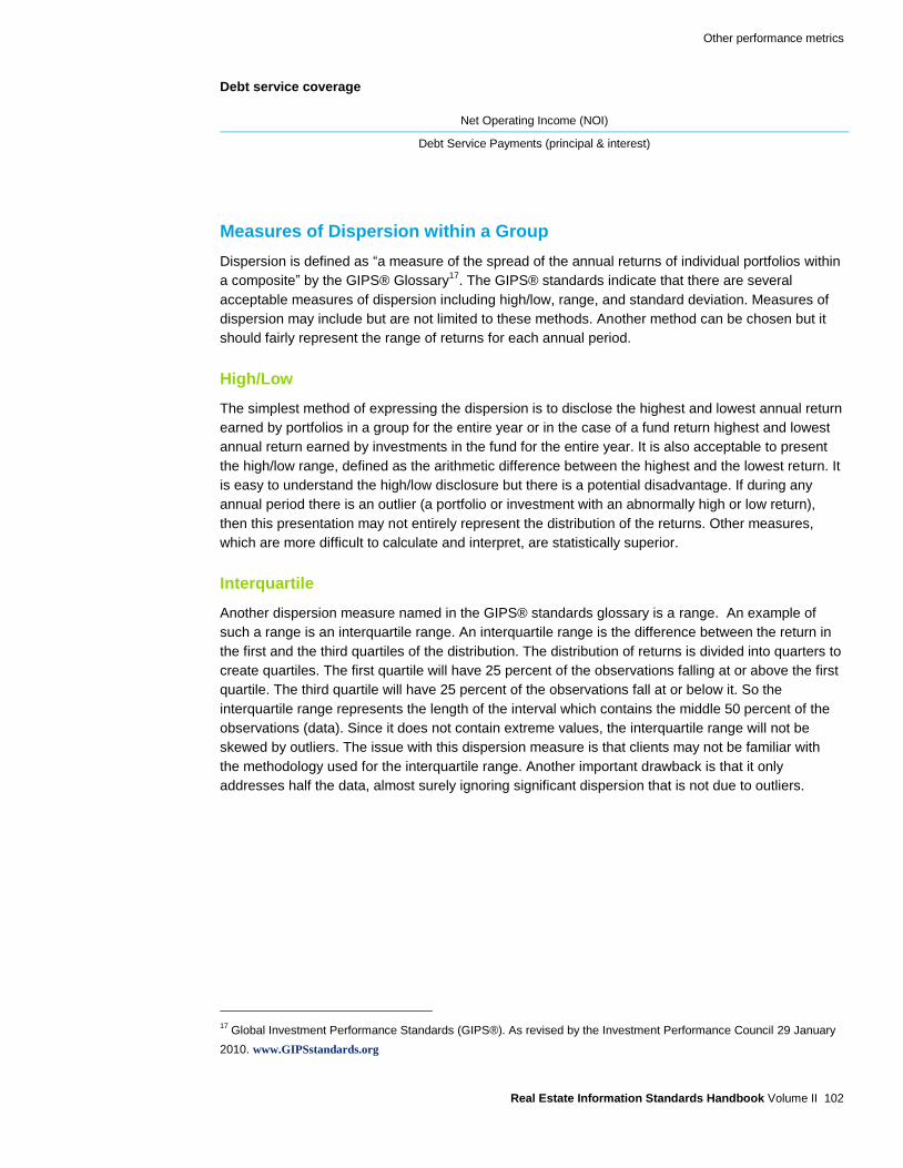
Other performance metrics
Real Estate Information Standards Handbook Volume II 102
Debt service coverage
Net Operating Income (NOI)
Debt Service Payments (principal & interest)
Measures of Dispersion within a Group
Dispersion is defined as “a measure of the spread of the annual returns of individual portfolios within
a composite” by the GIPS® Glossary17
. The GIPS® standards indicate that there are several
acceptable measures of dispersion including high/low, range, and standard deviation. Measures of
dispersion may include but are not limited to these methods. Another method can be chosen but it
should fairly represent the range of returns for each annual period.
High/Low
The simplest method of expressing the dispersion is to disclose the highest and lowest annual return
earned by portfolios in a group for the entire year or in the case of a fund return highest and lowest
annual return earned by investments in the fund for the entire year. It is also acceptable to present
the high/low range, defined as the arithmetic difference between the highest and the lowest return. It
is easy to understand the high/low disclosure but there is a potential disadvantage. If during any
annual period there is an outlier (a portfolio or investment with an abnormally high or low return),
then this presentation may not entirely represent the distribution of the returns. Other measures,
which are more difficult to calculate and interpret, are statistically superior.
Interquartile
Another dispersion measure named in the GIPS® standards glossary is a range. An example of
such a range is an interquartile range. An interquartile range is the difference between the return in
the first and the third quartiles of the distribution. The distribution of returns is divided into quarters to
create quartiles. The first quartile will have 25 percent of the observations falling at or above the first
quartile. The third quartile will have 25 percent of the observations fall at or below it. So the
interquartile range represents the length of the interval which contains the middle 50 percent of the
observations (data). Since it does not contain extreme values, the interquartile range will not be
skewed by outliers. The issue with this dispersion measure is that clients may not be familiar with
the methodology used for the interquartile range. Another important drawback is that it only
addresses half the data, almost surely ignoring significant dispersion that is not due to outliers.
17
Global Investment Performance Standards (GIPS®). As revised by the Investment Performance Council 29 January
2010. www.GIPSstandards.org

Other performance metrics
Real Estate Information Standards Handbook Volume II 103
Standard deviation
Standard deviation is the most commonly accepted measure of dispersion. In groups, the standard
deviation measures the cross-sectional dispersion of returns to portfolios. Standard deviation for a
group in which the constituent portfolios are equally weighted is:
where ri is the return of each individual portfolio
rc is the equal-weighted mean or arithmetic mean return of the portfolios in the group
n is, the number of portfolios in the group.
If the individual portfolio returns are normally distributed around the mean return, then approximately
two-thirds of the portfolios will have returns falling between the mean plus the standard deviation
and the mean minus the standard deviation.
The standard deviation of portfolio returns is a valid measure of group dispersion. Most spreadsheet
programs include statistical functions to facilitate the calculation (such as the STDEV function in
Microsoft Excel), and many clients will have at least a passing acquaintance with the concept of a
standard deviation.
At a minimum, quarterly data points should be used for calculating the standard deviation since
valuations are presumed to be completed on a quarterly basis. The resulting quarterly calculation
should be annualized accordingly using the formula [Quarterly Result x 4 ^ (1/2))]. The NFI-ODCE
only reports standard deviations for periods containing at least 20 full quarters (five years) as any
measurements of smaller time periods are thought to produce results that are statistically
insignificant.
Risk measures
There are several ratios that can be used to evaluate fund performance and to measure and
compare portfolio risk. Please note that the measures listed below are widely used in financial
circles but their applicability to real estate is debatable, so use with caution. Real estate returns are
typically asymmetric, and certain measures of dispersion (i.e. standard deviation) that are used in
the risk measures below are thought to be most suitable for investments that have normal expected
return distributions.
Sharpe ratio
The Sharpe Ratio was invented by Nobel Laureate and U.S. Economist William Sharpe. It can be
calculated for expected returns or for historic returns. It is a ratio defined as the performance in

Other performance metrics
Real Estate Information Standards Handbook Volume II 104
excess of the risk-free rate divided by the volatility of the returns as measured by the standard
deviation of the portfolio’s return:
Risk free rates are typically presumed to be U.S. treasury rates. Sharpe ratios should also be shown
on an annualized basis. For example, if monthly performance is used in the above calculation,
multiply the calculated Sharpe ratio by the square root of 12 to annualize the ratio. The higher the
Sharpe ratio, the better the fund’s historical risk-adjusted performance. A ratio of 1.0 indicates one
unit of return per unit of risk; 2.0 indicates two units of return per unit of risk. Negative values
indicate loss, or that a disproportionate amount of risk was taken to generate positive returns.
Generally, a measure of above 1 is considered good, and above 3 is considered excellent.
Treynor ratio — (also known as the reward to volatility ratio)
The Treynor Ratio (also known as the Reward to Volatility Ratio) measures returns earned in excess
of that which could have been earned on a riskless investment per each unit of market risk. It is
similar to the Sharpe ratio, but uses beta as the measure of volatility.
Where Equals
_ rp
Average return of the portfolio
_ rf
Average return of the risk-free investment
p Beta of the portfolio

Other performance metrics
Real Estate Information Standards Handbook Volume II 105
Tracking error
The Tracking Error measures how closely a portfolio performs compared to its benchmark. Tracking
errors are typically only reported for periods of greater than five years, because of the volatility in
shorter period returns. Although there are several variations of the tracking error formula, the most
commonly used in our industry simply calculates the standard deviation of the difference between
the return of the fund and the benchmark. The statistical formula is:
σ2 = 1/(n - 1) Σ(xi - yi)
2
Where σ is the tracking error
n is the number of periods over which it is measured
x is the percentage return on the portfolio in period i
y is the percentage return on the benchmark
Tracking error percentages should also be shown on an annualized basis. For example, if quarterly
performance is used in the spreadsheet calculation, multiply the calculated Tracking Error by the
square root of 4 to annualize the results. Assuming normal distribution of the return differences, the
Tracking Errors can be used to set general returns expectations. For example, a Tracking Error of
.02 would indicate that 66.7% of the time, the return would be within +/- 2% of the benchmark return.
Correlation
Correlation is a statistical measure of the degree to which two investments move relative to one
another. This measure is often used when comparing portfolio returns against appropriate
benchmarks. The Spearman’s Rho correlation is frequently used as it is nonparametric and requires
no normal distribution:
The correlation calculation will always yield a value between -1.0 and +1.0. A minimum of ten
periods must be used in for the correlation calculation to be statistically significant. A perfect
correlation of +1 indicates that both investments always move together, whereas a correlation of 0
indicates there is no relationship between the two, and a negative correlation indicates an inverse
relationship between the two. It is important to note that when calculating the correlation of a fund’s
return to a benchmark’s return, the result does not necessarily indicate the degree of
out/underperformance, but rather can only be used to predict that the returns move in the same or
opposite direction as the benchmark.
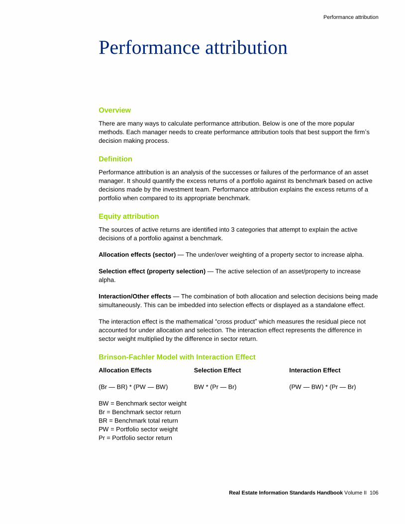
Performance attribution
Real Estate Information Standards Handbook Volume II 106
Performance attribution
Overview
There are many ways to calculate performance attribution. Below is one of the more popular
methods. Each manager needs to create performance attribution tools that best support the firm’s
decision making process.
Definition
Performance attribution is an analysis of the successes or failures of the performance of an asset
manager. It should quantify the excess returns of a portfolio against its benchmark based on active
decisions made by the investment team. Performance attribution explains the excess returns of a
portfolio when compared to its appropriate benchmark.
Equity attribution
The sources of active returns are identified into 3 categories that attempt to explain the active
decisions of a portfolio against a benchmark.
Allocation effects (sector) — The under/over weighting of a property sector to increase alpha.
Selection effect (property selection) — The active selection of an asset/property to increase
alpha.
Interaction/Other effects — The combination of both allocation and selection decisions being made
simultaneously. This can be imbedded into selection effects or displayed as a standalone effect.
The interaction effect is the mathematical “cross product” which measures the residual piece not
accounted for under allocation and selection. The interaction effect represents the difference in
sector weight multiplied by the difference in sector return.
Brinson-Fachler Model with Interaction Effect
Allocation Effects Selection Effect Interaction Effect
(Br — BR) * (PW — BW) BW * (Pr — Br) (PW — BW) * (Pr — Br)
BW = Benchmark sector weight
Br = Benchmark sector return
BR = Benchmark total return
PW = Portfolio sector weight
Pr = Portfolio sector return

Performance attribution
Real Estate Information Standards Handbook Volume II 107
Brinson-Fachler Model without Interaction Effect
Allocation Effects (includes interaction effects) Selection Effect
(Br — BR) * (PW — BW) PW * (Pr — Br)
BW = Benchmark sector weight
Br = Benchmark sector return
BR = Benchmark total return
PW = Portfolio sector weight
Pr = Portfolio sector return
Contribution/Absolute attribution
Contribution Effect aims to quantify an assets and sectors contribution to the total return of the fund.
It does not compare the performance against a benchmark but instead looks to how much each
asset/sector contributed to the fund’s total return. It should always equal the portfolio’s total return.
Contribution effect
(PW * PR)
PW = Portfolio weight
PR = Portfolio return
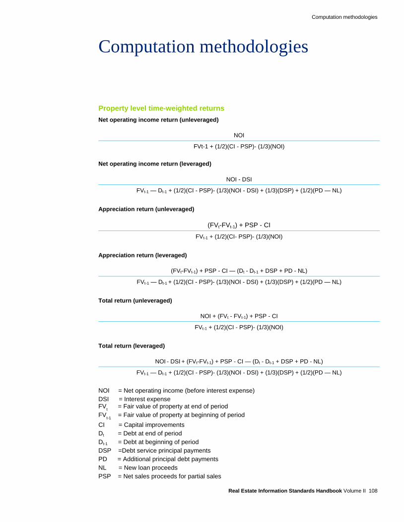
Computation methodologies
Real Estate Information Standards Handbook Volume II 108
Computation methodologies
Property level time-weighted returns
Net operating income return (unleveraged)
NOI
FVt-1 + (1/2)(CI - PSP)- (1/3)(NOI)
Net operating income return (leveraged)
NOI - DSI
FVt-1 — Dt-1 + (1/2)(CI - PSP)- (1/3)(NOI - DSI) + (1/3)(DSP) + (1/2)(PD — NL)
Appreciation return (unleveraged)
(FVt-FVt-1) + PSP - CI
FVt-1 + (1/2)(CI- PSP)- (1/3)(NOI)
Appreciation return (leveraged)
(FVt-FVt-1) + PSP - CI — (Dt - Dt-1 + DSP + PD - NL)
FVt-1 — Dt-1 + (1/2)(CI - PSP)- (1/3)(NOI - DSI) + (1/3)(DSP) + (1/2)(PD — NL)
Total return (unleveraged)
NOI + (FVt - FVt-1) + PSP - CI
FVt-1 + (1/2)(CI - PSP)- (1/3)(NOI)
Total return (leveraged)
NOI - DSI + (FVt-FVt-1) + PSP - CI — (Dt - Dt-1 + DSP + PD - NL)
FVt-1 — Dt-1 + (1/2)(CI - PSP)- (1/3)(NOI - DSI) + (1/3)(DSP) + (1/2)(PD — NL)
NOI = Net operating income (before interest expense)
DSI = Interest expense FV
t = Fair value of property at end of period
FVt-1
= Fair value of property at beginning of period
CI = Capital improvements
Dt = Debt at end of period
Dt-1 = Debt at beginning of period
DSP =Debt service principal payments
PD = Additional principal debt payments
NL = New loan proceeds
PSP = Net sales proceeds for partial sales

Computation methodologies
Real Estate Information Standards Handbook Volume II 109
Investment level time-weighted returns
Net investment income return (before fee, leveraged)
NII + AF + IFE
NAVt-1 + TWC - TWD
Net investment income return (after fee, leveraged)
NII
NAVt-1 + TWC - TWD
Appreciation return (before fee, leveraged)
Real Estate Appreciation + Debt Appreciation
NAVt-1 + TWC - TWD
Appreciation return (after fee, leveraged)
Real Estate Appreciation + Debt Appreciation - IFC
NAVt-1 + TWC - TWD
Total return (before fee, leveraged)
NII + AF + IFE + Real Estate Appreciation + Debt Appreciation
NAVt-1 + TWC - TWD
Total return (after fee, leveraged)
NII + Real Estate Appreciation + Debt Appreciation - IFC
NAVt-1 + TWC - TWD
NII = Net investment income (after interest expense, advisory fees and expensed incentive fees)
AF = Advisory fee expense
IFE = Incentive fee expense
IFC = Change in capitalized incentive fee
NAVt-1 = Net asset value of investment at beginning of period
TWC = Time weighted contributions
TWD = Time weighted distributions

Computation methodologies
Real Estate Information Standards Handbook Volume II 110
Fund level time-weighted returns
Net investment income return (before fee, leveraged)
NII + AF + IFE
NAVt-1 + TWC - TWD
Net investment income return (after fee, leveraged)
NII
NAVt-1 + TWC - TWD
Appreciation return (before fee, leveraged)
Real Estate Appreciation + Debt Appreciation
NAVt-1 + TWC - TWD
Appreciation return (after fee, leveraged)
Real Estate Appreciation + Debt Appreciation - IFC
NAVt-1 + TWC - TWD
Total return (before fee, leveraged)
NII + AF + IFE + Real Estate Appreciation + Debt Appreciation
NAVt-1 + TWC - TWD
Total return (after fee, leveraged)
NII + Real Estate Appreciation + Debt Appreciation - IFC
NAVt-1 + TWC - TWD
NII = Net investment income (after interest expense)
AF = Advisory fee expense
IFE = Incentive fee expense
IFC = Change in capitalized incentive fee
NAVt-1 = Net asset value of investment at beginning of period
TWC = Time weighted contributions
TWD = Time weighted distributions
Sample IRR formula
F0 + F1 + F2 + F3 +... + Fx = 0
1+IRR (1+IRR)2 (1+IRR)
3 (1+IRR)
n

Computation methodologies
Real Estate Information Standards Handbook Volume II 111
Investment multiple or total value to paid-in capital multiple (TVPI)
TV
PIC
TV = Total value
Fund: Sum of residual fund net assets (NAV) plus aggregate fund distributions
Investment: Sum of residual investment net assets (NAV) plus aggregate distributions
Property: Sum of property fair value (net of debt) plus aggregate distributions (note: if actual
property distributions are not separately maintained, estimates can be calculated by
aggregating the property’s net operating income (after interest expense) and
subtracting principal payments).
PIC = Paid in capital
Fund: Cumulative capital contributed to the fund
Investment: Cumulative capital contributed to the investment
Property: Cash invested in the property (cash at acquisition plus capital additions)
Realization multiple or cumulative distributions to paid-in capital multiple (DPI)
D
PIC
D = Total distributions
Fund: Aggregate fund distributions paid since inception
Investment: Aggregate investment distributions paid since inception
Property: Aggregate property distributions paid since inception (note: if actual property
distributions are not separately maintained, estimates can be calculated by
aggregating the property’s net operating income (after interest expense) and
subtracting principal payments).
PIC = Paid in capital
Fund: Cumulative capital contributed to the fund
Investment: Cumulative capital contributed to the investment
Property: Cash invested in the property (cash at acquisition plus capital additions)
Paid-in capital multiple or paid-in capital to committed capital multiple (PIC)
PIC
CC
PIC = Paid in capital
Fund: Cumulative capital contributed to the fund
Investment: Cumulative capital contributed to the investment
Property: Cash invested in the property (cash at acquisition plus capital additions)
CC = Committed capital
Fund: Cumulative fund PIC plus unfunded capital
Investment: Cumulative investment PIC plus unfunded capital
Property: Cumulative property PIC plus unfunded commitments (e.g. renovation reserves)

Computation methodologies
Real Estate Information Standards Handbook Volume II 112
Residual multiple or residual value to paid-in capital (RVPI)
RV
PIC
RV = Residual value
Fund: Net asset value (NAV) of the fund
Investment: Net asset value (NAV) of the investment
Property: Property fair value net of debt
PIC = Paid in capital
Fund: Cumulative capital contributed to the fund
Investment: Cumulative capital contributed to the investment
Property: Cash invested in the property (cash at acquisition plus capital additions)
Distributed income formula
Distributed Income
Weighted Average Equity
Retained income formula
Retained Income
Weighted Average Equity
Distribution return formula
LP Distributions Net of Fees
LP Weighted Average Equity
Price change return formula
LP NAV1 ex distribution — LP NAV
0 ex previous quarter distribution + LP redemptions — LP Contributions
LP Weighted Average Equity
Leverage risk ratio
Total Third Party Debt
Total Gross Assets
Debt ratio — Investment company guide calculation (non-operating model)
Wholly owned debt (property & fund) + fund’s economic share of JV debt
Total Assets + fund’s share of total JV liabilities
Debt ratio — Consolidated balance sheet calculation (operating model)
Wholly owned debt (property & fund) + fund’s economic share of JV debt
Total Assets — JV partner economic share of RE Partnership Assets
Debt service coverage ratio
Net Operating Income (NOI)
Debt Service Payments (principal and interest)

Sample disclosures
Real Estate Information Standards Handbook Volume II 113
Sample disclosures
These disclosures are intended to be used in performance presentations for U.S., institutional real
estate assets. Disclosures, like the one listed below, would typically accompany any performance
presentation that is made in a client report.
Property level disclosures
Unleveraged property level performance return [EXAMPLE]
Performance results are before the effect of leverage and calculated using the Property-Level
return methodology outlined in the Real Estate Information Standards (“REIS’) Performance
Measurement Resource Manual.
Performance results are before deduction of advisor asset management and performance
incentive fees and after deduction of advisor acquisition fees.
Performance results are before the effect of operating partner/joint venture partner fees and
distribution waterfalls. (Only use if applicable.)
Performance results do not include cash and cash equivalents, related interest income and other
non-property related income and expenses.
The inputs to the performance return calculation are calculated in accordance with the Real Estate
Information Standards (“REIS”). The Net Operating Income component of the return is based on
accrual recognition of earned income. Capital expenditures, tenant improvements, and lease
commissions are capitalized and included in the cost of the property; are not amortized; and are
reconciled through the valuation process and reflected in the capital return (appreciation)
component.
Annual performance returns are time-weighted, calculated by geometrically linking quarterly
returns. Income and capital returns may not equal total returns due to compounding effects of
linking the quarterly returns.
The time-weighted return calculations begin on the acquisition date for each property and end on
the disposition date. Partial periods are not dropped.
If a property level internal rate of return (“IRR”) is presented, a disclosure describing the calculation
methodology is needed. Please refer to section 7.10 for a sample disclosure.
Leveraged property level performance return [EXAMPLE]
Same as above except for the first disclosure.
Performance results are after the effect of leverage and calculated using the Property-Level return
methodology outlined in the Real Estate Information Standards (“REIS’) Performance
Measurement Resource Manual.

Sample disclosures
Real Estate Information Standards Handbook Volume II 114
Property level valuation policy [EXAMPLE]
If presenting performance on a stand-alone basis (not in conjunction with financial statements) a
valuation policy should be disclosed. Otherwise, reference can be made to the accompanying
financial statement footnotes.
Real property assets are internally valued quarterly by the manager and appraised no less
frequently than every three years by an independent member of the Appraisal Institute.
Both the internal and external property valuations rely primarily on the application of market
discount rates to future projections of unleveraged cash flows and capitalized terminal values over
the expected holding period of each property.
Property mortgages, notes, and loans with maturities greater than one year from the date of the
balance sheet are marked to market using prevailing interest rates for comparable property loans.
Loan repayment fees, if any, are considered in the projected year of sale.
Property level benchmark disclosure [EXAMPLE]
The benchmark for this group is the National Council of Real Estate Investment Fiduciaries
(“NCREIF”) Property Index (“NPI”).
The NPI benchmark has been taken from published sources.
The NPI is an unleveraged, before fee index of operating properties and, includes various
operating real estate property types, excludes cash and other non-property related assets and
liabilities, income, and expenses.
The calculation methodology for the NPI is consistent with the calculation methodology for all
properties presented herein.
The NPI data, once aggregated, may not be comparable to the performance of the properties
presented herein due to current and historical differences in portfolio composition by asset size,
geographic location and property type.
Investment level disclosures
Investment level represents a discrete asset or group of assets held for income, appreciation, or
both and tracked separately. Investment level performance is typically presented at the fund level.
Please refer to the disclosure section below.
Fund level disclosures
Unleveraged fund level performance return [EXAMPLE]
Hypothetical, unleveraged fund returns are often presented as supplemental reporting. To calculate
these returns, adjustments to the numerator are made which remove interest expense and
appreciation related to the value of the debt. Adjustments to the denominator are made which
increase contributions and distributions by the amount of debt placed, loan fees incurred, interest
expensed and debt repaid. The disclosures follow those described in the disclosure section below,
except for the first bullet point, which is replaced with a description of the assumptions used to de-
lever the portfolio.
Leveraged fund level performance return [EXAMPLE]
Performance results are presented net of leverage.
Performance results include cash and cash equivalents and related interest income.
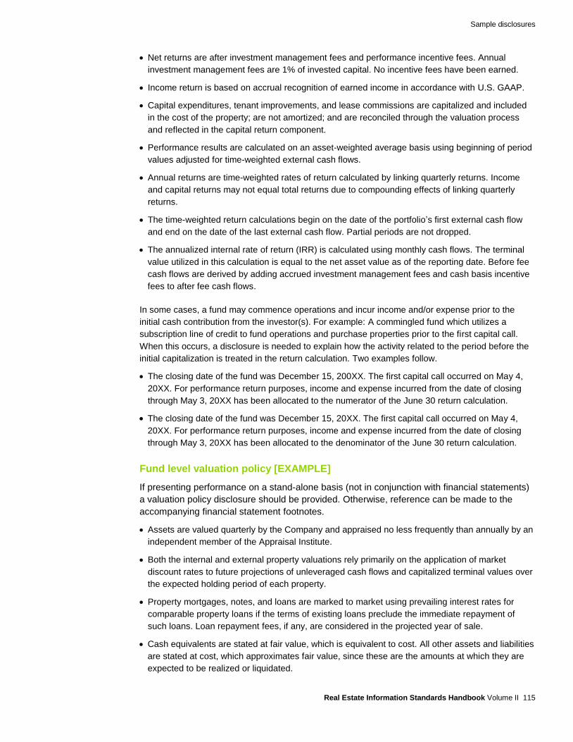
Sample disclosures
Real Estate Information Standards Handbook Volume II 115
Net returns are after investment management fees and performance incentive fees. Annual
investment management fees are 1% of invested capital. No incentive fees have been earned.
Income return is based on accrual recognition of earned income in accordance with U.S. GAAP.
Capital expenditures, tenant improvements, and lease commissions are capitalized and included
in the cost of the property; are not amortized; and are reconciled through the valuation process
and reflected in the capital return component.
Performance results are calculated on an asset-weighted average basis using beginning of period
values adjusted for time-weighted external cash flows.
Annual returns are time-weighted rates of return calculated by linking quarterly returns. Income
and capital returns may not equal total returns due to compounding effects of linking quarterly
returns.
The time-weighted return calculations begin on the date of the portfolio’s first external cash flow
and end on the date of the last external cash flow. Partial periods are not dropped.
The annualized internal rate of return (IRR) is calculated using monthly cash flows. The terminal
value utilized in this calculation is equal to the net asset value as of the reporting date. Before fee
cash flows are derived by adding accrued investment management fees and cash basis incentive
fees to after fee cash flows.
In some cases, a fund may commence operations and incur income and/or expense prior to the
initial cash contribution from the investor(s). For example: A commingled fund which utilizes a
subscription line of credit to fund operations and purchase properties prior to the first capital call.
When this occurs, a disclosure is needed to explain how the activity related to the period before the
initial capitalization is treated in the return calculation. Two examples follow.
The closing date of the fund was December 15, 200XX. The first capital call occurred on May 4,
20XX. For performance return purposes, income and expense incurred from the date of closing
through May 3, 20XX has been allocated to the numerator of the June 30 return calculation.
The closing date of the fund was December 15, 20XX. The first capital call occurred on May 4,
20XX. For performance return purposes, income and expense incurred from the date of closing
through May 3, 20XX has been allocated to the denominator of the June 30 return calculation.
Fund level valuation policy [EXAMPLE]
If presenting performance on a stand-alone basis (not in conjunction with financial statements)
a valuation policy disclosure should be provided. Otherwise, reference can be made to the
accompanying financial statement footnotes.
Assets are valued quarterly by the Company and appraised no less frequently than annually by an
independent member of the Appraisal Institute.
Both the internal and external property valuations rely primarily on the application of market
discount rates to future projections of unleveraged cash flows and capitalized terminal values over
the expected holding period of each property.
Property mortgages, notes, and loans are marked to market using prevailing interest rates for
comparable property loans if the terms of existing loans preclude the immediate repayment of
such loans. Loan repayment fees, if any, are considered in the projected year of sale.
Cash equivalents are stated at fair value, which is equivalent to cost. All other assets and liabilities
are stated at cost, which approximates fair value, since these are the amounts at which they are
expected to be realized or liquidated.

Sample disclosures
Real Estate Information Standards Handbook Volume II 116
Fund level benchmark disclosure [EXAMPLE]
The benchmark for this group is the National Council of Real Estate Investment Fiduciaries
(“NCREIF”) Fund Index Open-Ended Diversified Core Equity (“NFI-ODCE”).
The NFI-ODCE benchmark has been taken from published sources.
The NFI-ODCE is a pre and post-fee index of open-ended funds with lower risk investment
strategies, utilizing low leverage and equity ownership of stable U.S. operating properties. The
index is capitalization-weighted, based on each fund’s net invested capital.
The NFI-ODCE data, once aggregated, may not be comparable to the performance of the
fund presented herein due to current and historical differences in portfolio composition by
asset size, geographic location, property type and degree of leverage.
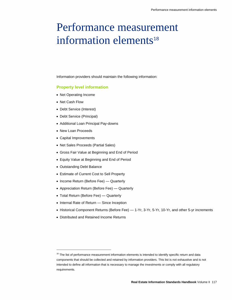
Performance measurement information elements
Real Estate Information Standards Handbook Volume II 117
Performance measurement
information elements18
Information providers should maintain the following information:
Property level information
Net Operating Income
Net Cash Flow
Debt Service (Interest)
Debt Service (Principal)
Additional Loan Principal Pay-downs
New Loan Proceeds
Capital Improvements
Net Sales Proceeds (Partial Sales)
Gross Fair Value at Beginning and End of Period
Equity Value at Beginning and End of Period
Outstanding Debt Balance
Estimate of Current Cost to Sell Property
Income Return (Before Fee) — Quarterly
Appreciation Return (Before Fee) — Quarterly
Total Return (Before Fee) — Quarterly
Internal Rate of Return — Since Inception
Historical Component Returns (Before Fee) — 1-Yr, 3-Yr, 5-Yr, 10-Yr, and other 5-yr increments
Distributed and Retained Income Returns
18
The list of performance measurement information elements is intended to identify specific return and data
components that should be collected and retained by information providers. This list is not exhaustive and is not
intended to define all information that is necessary to manage the investments or comply with all regulatory
requirements.
Performance measurement information elements
Real Estate Information Standards Handbook Volume II 118
Investment and fund level information
Net Investment Income
Fair Value at Beginning and End of Period
Capital Contributions — Amounts and Dates
Capital Distributions and Redemptions — Amounts and Dates
Capital Distributions Resulting from Financing and Investing Activities — Amounts and Dates
Investment Management Fees
Estimate of Current Costs to Sell Investments
Weighted Average Equity
Capital Appreciation
Paid in Capital
Income Return (Before and After Fee) — Quarterly
Appreciation Return (Before and After Fee) — Quarterly
Total Return (Before and After Fee) — Quarterly
Internal Rate of Return — Since Inception
Historical Component Returns (Before and After Fee) — 1-Yr, 3-Yr, 5-Yr, 10-Yr, and other 5-yr
increments
Distributed and Retained Income Returns
Distribution and Price Change Returns

Appendices
Real Estate Information Standards Handbook Volume II 119
Appendices

Appendices
Real Estate Information Standards Handbook Volume II 120
Appendix A — Sample Fund Level Presentation for Client Reporting
XYZ FUND, L.P.
Historical Performance, 20XX-20XX Dollar Amounts in Thousands
Investment Realization
Appreciation Multiple Multiple
Year (Depreciation) (TVPI) (DPI) PIC RVPI
20XX 125,213$ 56 % % 6.15 % 3.00 9.15 % 13.06 % 5.15 % 3.00 % 8.15 % 1.03 - 0.24 1.03
20XX 449,809 37 6.07 7.00 13.07 21.39 5.07 7.00 12.07 1.24 - 0.73 1.24
20XX 562,550 28 6.45 8.00 14.45 16.32 5.45 8.00 13.45 1.44 0.19 0.90 1.25
20XX 532,547 19 6.19 8.00 14.19 15.97 5.19 8.00 13.19 1.68 0.61 1.00 1.07
20XX 265,460 16 5.45 (9.00) (3.55) (10.01) 4.45 (9.00) (4.55) 1.44 0.91 1.00 0.53
Annualized Time Weighted Returns
Since Inception (January 1, 20XX) 6.05 3.19 9.24 10.75 5.06 3.19 8.24
Annualized Internal Rate of Return
Since Inception (January 1, 20XX) 9.45 % 8.45 %
TVPI = Total Value to Paid-In Capital
DPI = Distributed Capital to Paid-In Capital
PIC = Paid-In Capital to Committed Capital
RVPI = Residual Value to Paid-In Capital
Notes:
1. Returns presented are net of leverage.
2. Performance results include cash and cash equivalents and related interest income.
3. Net returns are after investment management fees and performance incentive fees. Annual investment management fees are 1% of invested capital. No incentive fees have been earned.
4. The income return is based on accrual recognition of earned income.
5. Capital expenditures, tenant improvements and lease commissions are capitalized and included in the cost of the property; are not amortized; and are reconciled through the valuation process and
and reflected in the capital return component.
6. Performance results are calculated on an asset-weighted average basis using beginning of period values, adjusted for time-weighted external cash flows.
7. Annual returns are time-weighted rates of return calculated by linking quarterly returns. Income and capital returns may not equal total returns due to compounding effects of linking quarterly returns.
8. The time-weighted return calculations begin on the date of the portfolio’s first external cash flow and end on the date of the last external cash flow. Partial periods are not dropped.
9. The annualized internal rate of return ("IRR") is calculated using monthly cash flows. The terminal value utilized in this calculation is equal to the net asset value as of December 31, 20XX.
10. Assets are valued quarterly by the General Partner and appraised annually by an independent member of the Appraisal Institute.
11. Additional information, including the Fund's valuation policy, capitalization policy regarding capital expenditures, tenant improvements, lease commissions and information related to investment
management and incentive fees is presented in the notes accompanying the financial statements.
12. The National Council of Real Estate Investment Fiduciaries ("NCREIF") Fund Index Open-Ended Diversified Core Equity ("NFI-ODCE") has been taken from published sources. The NFI-ODCE is a
before-fee index of open-ended funds with lower risk investment strategies, utilizing low leverage and equity ownership of stable U.S. operating properties. The Index is capitalization-weighted, based
on each fund's net invested capital.
13. The NFI-ODCE data, once aggregated, may not be comparable to the performance of the XYZ Fund due to current and historical differences in portfolio composition by asset size, geographic location,
property type and degree of leverage.
Before Fee Returns
Index NetGross
TotalTotal
Multiples
ODCE
ReturnsBenchmark (Depreciation)Returns
Year End
After Fee Returns
Assets
Investment Percent
Leveraged
Net
Income (Loss)
Appreciation
NFI-
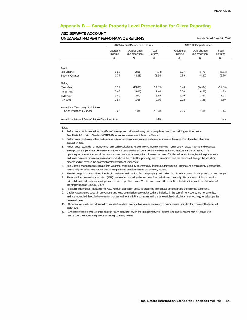
Appendices
Real Estate Information Standards Handbook Volume II 121
Appendix B — Sample Property Level Presentation for Client Reporting
ABC SEPARATE ACCOUNT
UNLEVERED PROPERTY PERFORMANCE RETURNS Periods Ended June 30, 20XX
Operating Appreciation Total Operating Appreciation Total
Income (Depreciation) Returns Income (Depreciation) Returns
% % % % % %
20XX
First Quarter 1.62 (2.56) (.94) 1.37 (8.70) (7.33)
Second Quarter 1.74 (3.28) (1.54) 1.50 (5.20) (6.70)
Rolling
One Year 6.19 (19.60) (14.35) 5.49 (24.04) (19.56)
Three Year 5.42 (3.80) 1.48 5.56 (4.39) .99
Five Year 5.60 3.01 8.75 6.05 1.50 7.61
Ten Year 7.54 1.65 9.30 7.18 1.26 8.50
Annualized Time-Weighted Return
Since Inception (9/9/XX) 8.29 1.86 10.28 7.75 1.60 9.44
Annualized Internal Rate of Return Since Inception 9.15 n/a
Notes:
1. Performance results are before the effect of leverage and calculated using the property level return methodology outlined in the
Real Estate Information Standards ("REIS") Performance Measurement Resource Manual.
2. Performance results are before deduction of advisor asset management and performance incentive fees and after deduction of advisor
acquisition fees.
3. Performance results do not include cash and cash equivalents, related interest income and other non-property related income and expenses.
4. The inputs to the performance return calculation are calculated in accordance with the Real Estate Information Standards ("REIS"). The
operating income component of the return is based on accrual recognition of earned income. Capitalized expenditures, tenant improvements
and lease commissions are capitalized and included in the cost of the property; are not amortized; and are reconciled through the valuation
process and reflected in the appreciation/ (depreciation) component.
5. Annualized performance returns are time-weighted, calculated by geometrically linking quarterly returns. Income and appreciation/ (depreciation)
returns may not equal total returns due to compounding effects of linking the quarterly returns.
6. The time-weighted return calculations begin on the acquisition date for each property and end on the disposition date. Partial periods are not dropped.
7. The annualized internal rate of return ("IRR") is calculated assuming that net cash flow is distributed quarterly. For purposes of this calculation,
net cash flow is defined as operating income minus capitalized costs. The terminal value utilized in this calculation is equal to the fair value of
the properties as of June 30, 2009.
8. Additional information, including the ABC Account's valuation policy, is presented in the notes accompanying the financial statements.
9. Capital expenditures, tenant improvements and lease commissions are capitalized and included in the cost of the property; are not amortized;
and are reconciled through the valuation process and for the NPI is consistent with the time-weighted calculation methodology for all properties
presented herein.
10. Performance results are calculated on an asset-weighted average basis using beginning of period values, adjusted for time-weighted external
cash flows.
11. Annual returns are time-weighted rates of return calculated by linking quarterly returns. Income and capital returns may not equal total
returns due to compounding effects of linking quarterly returns.
ABC Account Before Fee Returns NCREIF Property Index