Quantifying Steganographic Embedding Capacity in DCT-Based
Embedding Schemes
by
Anna Zawilska
BScEng (Electronic) Summa Cum Laude
Submitted in fulfilment of the requirements for the Degree of Master of Science in Electronic
Engineering in the School of Electrical, Electronic and Computer Engineering at the University
of KwaZulu-Natal, Durban
January 2012
Supervisor: Professor Roger Peplow

ii
Preface
The research discussed in this dissertation was done at the University of KwaZulu-Natal,
Durban from February 2011 until January 2012 by Anna Zawilska under the supervision of
Professor Roger Peplow.
As the candidate’s supervisor, I, Roger Peplow, approve this dissertation for submission.
Signed:
Date:
I, Anna Zawilska, declare that
i. The research reported in this dissertation/thesis, except where otherwise indicated, is
my original work.
ii. This dissertation/thesis has not been submitted for any degree or examination at any
other university.
iii. This dissertation/thesis does not contain other persons’ data, pictures, graphs or other
information, unless specifically acknowledged as being sourced from other persons.
iv. This dissertation/thesis does not contain other persons’ writing, unless specifically
acknowledged as being sourced from other researchers. Where other written sources
have been quoted, then:
(a) their words have been re-written but the general information attributed to them
has been referenced;
(b) where their exact words have been used, their writing has been placed inside
quotation marks, and referenced.
v. Where I have reproduced a publication of which I am an author, co-author or editor, I
have indicated in detail which part of the publication was actually written by myself
alone and have fully referenced such publications.
vi. This dissertation/thesis does not contain text, graphics or tables copied and pasted from
the Internet, unless specifically acknowledged, and the source being detailed in the
dissertation/thesis and in the References sections.
Signed:
Date:

iii
Acknowledgements
I would like to thank my supervisor, Professor Roger Peplow, for his time and energy in
providing insightful advice and encouraging me even when I doubted myself.
I wish to thank my family who have provided me with constant support and encouragement.
Their courage and wise words have been essential to my personal and academic development
and no number of thanks would ever be enough.
I would also like to thank all of the other staff and postgraduates at the department for their
guidance, fellowship and for the laughs.
iv
Abstract
Digital image steganography has been made relevant by the rapid increase in media sharing
over the Internet and has thus experienced a renaissance. This dissertation starts with a
discussion of the role of modern digital image steganography and cell-based digital image
stego-systems which are the focus of this work. Of particular interest is the fact that cell-based
stego-systems have good security properties but relatively poor embedding capacity. The main
research problem is stated as the development of an approach to improve embedding capacity
in cell-based systems.
The dissertation then tracks the development of digital image stego-systems from spatial and
naïve to transform-based and complex, providing the context within which cell-based systems
have emerged and re-states the research problem more specifically as the development of an
approach to determine more efficient data embedding and error coding schemes in cell-based
stego-systems to improve embedding capacity while maintaining security.
The dissertation goes on to describe the traditional application of data handling procedures
particularly relating to the likely eventuality of JPEG compression of the image containing the
hidden information (i.e. stego-image) and proposes a new approach. The approach involves
defining a different channel model, empirically determining channel characteristics and using
them in conjunction with error coding systems and security selection criteria to find data
handling parameters that optimise embedding capacity in each channel. Using these
techniques and some reasoning regarding likely cover image size and content, image-global
error coding is also determined in order to keep the image error rate below 1% while
maximising embedding capacity.
The performance of these new data handling schemes is tested within cell-based systems.
Security of these systems is shown to be maintained with an up to 7 times improvement in
embedding capacity. Additionally, up to 10% of embedding capacity can be achieved versus
simple LSB embedding. The 1% image error rate is also confirmed to be upheld.
The dissertation ends with a summary of the major points in each chapter and some
suggestions of future work stemming from this research.
v
Table of Contents
Preface ...........................................................................................................................................ii
Acknowledgements ....................................................................................................................... iii
Abstract ......................................................................................................................................... iv
Table of Contents ........................................................................................................................... v
Acronyms .................................................................................................................................... viii
List of Figures ................................................................................................................................ ix
List of Tables ................................................................................................................................. xii
Chapter 1. Introduction .......................................................................................................... 1
1.1 Definition of Steganography ......................................................................................... 2
1.2 History of Steganography .............................................................................................. 3
1.3 Steganalysis ................................................................................................................... 5
1.4 Digital Image Steganography ........................................................................................ 6
1.5 Research Problem Statement ....................................................................................... 8
1.6 Research Methodology ................................................................................................. 8
1.7 Dissertation Roadmap ................................................................................................... 9
1.8 Published Works ........................................................................................................... 9
Chapter 2. Digital Image Steganographic Systems ............................................................... 10
2.1 Classification of Steganographic Systems ................................................................... 10
2.1.1 Relationship between Secret Message and Cover Image ................................... 10
2.1.2 Key Type .............................................................................................................. 11
2.1.3 Role of the Warden ............................................................................................. 12
2.2 Stego-System Model ................................................................................................... 12
2.3 Pertinent Properties of Stego-Systems ....................................................................... 14
2.3.1 Primary Attributes ............................................................................................... 14
2.3.2 Detectability versus Imperceptibility .................................................................. 16
2.4 Taxonomy of Digital Image Steganography ................................................................ 18
2.4.1 Spatial Domain Steganography ........................................................................... 19
vi
2.4.2 Transform Domain Steganography ..................................................................... 29
2.5 Discussion of Cell-Based Systems................................................................................ 49
2.6 Summary ..................................................................................................................... 50
Chapter 3. Formalising and Quantifying the Embedding Process ........................................ 52
3.1 The Channel Concept .................................................................................................. 52
3.2 Coefficient Movement & Previous Delta Values ......................................................... 57
3.2.1 Coefficient Movement ........................................................................................ 57
3.2.2 Delta Values used in YASS/MULTI ....................................................................... 67
3.3 Determining Channel Data Handling Parameters Graphically .................................... 70
3.4 Channel Characterisation ............................................................................................ 73
3.4.1 Determining Channel Characteristics Empirically ............................................... 73
3.5 Per Channel Determination of Optimal Delta ............................................................. 82
3.6 Compensation for Errors ............................................................................................. 84
3.6.1 Error Correction Selection ................................................................................... 84
3.6.2 Usable Channels & Per Channel Error Correction ............................................... 89
3.6.3 Image-Global Error Coding .................................................................................. 93
3.7 Selecting Error Coding Parameters for YASS2/MULTI2 ............................................... 99
3.8 Summary ................................................................................................................... 103
Chapter 4. Analysis of the Scheme ..................................................................................... 105
4.1 Steganalysis ............................................................................................................... 105
4.1.1 Detection Rate .................................................................................................. 105
4.1.2 Resistance against PF-274 ................................................................................. 106
4.2 Image Error Rate ....................................................................................................... 109
4.3 Embedding Capacity .................................................................................................. 110
4.3.2 Capacity as a Proportion of Image Size ............................................................. 114
4.4 Summary ................................................................................................................... 115
Chapter 5. Conclusion ......................................................................................................... 116
5.1 Summary of Dissertation ........................................................................................... 116

vii
5.1.1 Chapter 1 ........................................................................................................... 116
5.1.2 Chapter 2 ........................................................................................................... 118
5.1.3 Chapter 3 ........................................................................................................... 120
5.1.4 Chapter 4 ........................................................................................................... 122
5.2 Concluding Comments .............................................................................................. 123
5.3 Future Work .............................................................................................................. 124
References................................................................................................................................. 125
viii
Acronyms
Joint Photographic Experts Group JPEG
Mean Square Error MSE
Peak Signal to Noise Ratio PSNR
Red, Green and Blue RGB
Least Significant Bit LSB
Pseudo-random Number Generator PRNG
Least Significant Bit Matching LSBM
Least Significant Bit Matching Revisited LSBMR
Bit Plane Complexity Steganography BPCS
Discrete Cosine Transform DCT
Inverse Discrete Cosine Transform IDCT
Discrete Wavelet Transform DWT
Yet Another Steganographic System YASS
Repeat-Accumulate RA
Quantisation Index Modulation QIM
Forward Error Correcting FEC
Bose, Chaudhuri and Hocquenghem BCH
Cycle Redundancy Check CRC
ix
List of Figures
Figure 1-1. Proportion of cover types used in digital stego-applications ..................................... 7
Figure 2-1. Overview of stego-system ........................................................................................ 13
Figure 2-2. Sample image with a clear visual distortion (a) and after JPEG compression (b) ..... 15
Figure 2-3. Grey scale image and 5x5 pixel segment with corresponding pixel values .............. 20
Figure 2-4. LSB embedding.......................................................................................................... 22
Figure 2-5. Secret image (a) and cover image (b) ....................................................................... 22
Figure 2-6. Stego-image using LSB embedding with a small secret message ............................. 23
Figure 2-7. LSB plane of stego-image (a) and original cover image (b) ...................................... 23
Figure 2-8. Portion of image histogram before (a) and after (b) LSB embedding ...................... 24
Figure 2-9. Original cover image (a) and ‘bleeding effect’ due to too aggressive embedding (b)
..................................................................................................................................................... 25
Figure 2-10. Original image (a) and non-adaptive dithering (b) ................................................. 25
Figure 2-11. 5x5 pixel block in spatial domain (a) and its DCT (b) .............................................. 30
Figure 2-12. Illustration of physical significance of DCT ............................................................. 31
Figure 2-13. Original example image .......................................................................................... 32
Figure 2-14. Example image Figure 2-13 with 13% of highest frequency DCT coefficients set to 0
(a), 80% of highest frequency DCT coefficients set to 0 (b) and 4 lowest frequency DCT
coefficients reduced by 10 (c) ..................................................................................................... 32
Figure 2-15. Sample of an image with two overlapping blocks over which the DCT could be
taken ........................................................................................................................................... 32
Figure 2-16. Image showing 8x8 grid blocks used during JPEG compression ............................. 33
Figure 2-17. Zigzag ordering used during JPEG ........................................................................... 34
Figure 2-18. Standard JPEG quantisation matrix ( ) ......................................................... 35
Figure 2-19. JPEG quantisation =70 (a) and =30 (b) ........................................... 37
Figure 2-20. Sample image .......................................................................................................... 38
Figure 2-21. Decompressed images using JPEG compression with = 80 (a), 10 (b), 5 (c)
..................................................................................................................................................... 38
Figure 2-22. YASS grid ................................................................................................................. 43
Figure 2-23. BLOCKING and EMBED phases ................................................................................ 44
Figure 2-24. Lattices to embed one-bit data using QIM ............................................................. 46
Figure 2-25. QIM data embedding and retrieval ........................................................................ 46
Figure 2-26. Sample image with clear artefacts of alteration of DC DCT coefficient ................. 48
Figure 2-27. MULTI grid ............................................................................................................... 49
x
Figure 3-1. Traditional channel model in YASS ........................................................................... 53
Figure 3-2. Traditional channel model in YASS reordered column-by-column ........................... 53
Figure 3-3. Proposed channel model in YASS ............................................................................. 55
Figure 3-4. Proposed channel model in MULTI ........................................................................... 56
Figure 3-5. JPEG-GRID block grid ................................................................................................. 58
Figure 3-6. EMBED phase for JPEG-GRID .................................................................................... 58
Figure 3-7. Portion of COMPRESSION phase for JPEG-GRID ....................................................... 59
Figure 3-8. Upper limit on DCT coefficient movement using =50 plotted column-by-column
..................................................................................................................................................... 60
Figure 3-9. Upper limit on DCT coefficient movement using =50 plotted in a zigzag order . 60
Figure 3-10. EMBED phase for MULTI ......................................................................................... 61
Figure 3-11. COMPRESSION phase for MULTI............................................................................. 61
Figure 3-12. Example 11x11 DCT Coefficients of E-block ............................................................ 63
Figure 3-13. Spatial representation of 11x11 E-block ................................................................. 63
Figure 3-14. DCT of top left 8x8 segment of E-block .................................................................. 63
Figure 3-15. Random sample of 16 images taken from image database ................................... 65
Figure 3-16. Images used to produce results in Figure 3-18 and Figure 3-19 ............................. 66
Figure 3-17. Quantisation matrix for a quality factor of 80 ........................................................ 66
Figure 3-18. Histograms of coefficient movement for channels 2 (a) and 15 (b) for =80 for
JPEG-GRID ................................................................................................................................... 67
Figure 3-19. Histograms of coefficient movement for channels 2 (a) and 15 (b) for =80 for
MULTI .......................................................................................................................................... 67
Figure 3-20. Histogram of channel 15 movement for =80 for JPEG-GRID ............................. 71
Figure 3-21. Overview of effects on embedding capacity versus delta ...................................... 72
Figure 3-22. Scatter plot for channel 3 error rate and embedding rate over 1334 E-blocks...... 77
Figure 3-23. Scatter plot for channel 3 error rate and embedding rate over 26680 E-blocks.... 78
Figure 3-24. Scatter plot for channel 20 error rate and embedding rate over 26680 E-blocks . 79
Figure 3-25. Error rate tolerance lines for channel 3 .................................................................. 80
Figure 3-26. Channel 3 characteristics for one image (1334 E-blocks) (a) and for ten images
(13340 E-blocks) (b) .................................................................................................................... 80
Figure 3-27. Channel 3 characteristics for twenty images (26680 E-blocks) (a) and for thirty
images (40020 E-blocks) (b) ........................................................................................................ 80
Figure 3-28. Channel 20 characteristics for thirty images (40020 E-blocks) ............................... 81
Figure 3-29. Channel 60 characteristics for thirty images (40020 E-blocks) ............................... 81
Figure 3-30. Net payload including BCH coding for various channels ........................................ 83
xi
Figure 3-31. Channel-wise BCH encoding ................................................................................... 88
Figure 3-32. 12x12 matrix showing channels appropriate for data carrying .............................. 91
Figure 3-33. Net payload for channel 3 given BCH codes at =63 and =255 ...................... 92
Figure 3-34. Global BCH encoding .............................................................................................. 94
Figure 3-35. with mixed =64 and 31 ........................................................................... 101
Figure 3-36. with mixed =64 and 31 ........................................................................... 101
Figure 3-37. Final proposed ............................................................................................... 102
Figure 3-38. Final proposed ............................................................................................... 103
Figure 4-1. Delta values used in YASS with =50 (a) and from Chapter 3 (b) ........................ 109
Figure 4-2. Histogram of the number of times increase in embedding capacity over a YASS
system with =75 and =50 (a) and =75 (b) ................................................................. 112
Figure 4-3. Delta values used in YASS with =75 (a) and in YASS2 (b) .................................. 112
Figure 4-4. Example image where least improvement in embedding capacity is made .......... 113
Figure 4-5. Example image where most improvement in embedding capacity is made .......... 113
Figure 4-6. Histogram of the number of times increase in embedding capacity over a YASS
system for large images with =75 and =50 (a) and =75 (b) ...................................... 114
xii
List of Tables
Table 2-1. Compression ratio corresponding to a JPEG quality factor ....................................... 38
Table 3-1. Six BCH code combinations ........................................................................................ 92
Table 3-2. Global error correcting parameters for small and medium images at different
tolerance levels ........................................................................................................................... 97
Table 3-3. Generator polynomials of some common standards in CRC codes ........................... 98
Table 3-4. Characteristics of embedding capacity for small images using a tolerance limit of
98% for several .................................................................................................................. 100
Table 3-5. Characteristics of embedding capacity for medium images using a tolerance limit of
98% for several .................................................................................................................. 100
Table 3-6. Characteristics of embedding capacity for small images using a tolerance limit of
98% for two ....................................................................................................................... 102
Table 3-7. Characteristics of embedding capacity for medium images using a tolerance limit of
98% for two ....................................................................................................................... 102
Table 4-1. Performance of YASS against PF-274 ....................................................................... 108
Table 4-2. Performance of MULTI against PF-274 .................................................................... 108
Table 4-3. Performance of YASS2 against PF-274 ..................................................................... 108
Table 4-4. Performance of MULTI2 against PF-274 .................................................................. 108
Table 4-5. Embedding Capacity for MULTI2 and YASS2 as a percentage of number of image
pixels ......................................................................................................................................... 115
1
Chapter 1. Introduction
If all of the users of Facebook formed a country, it would be the third most highly populated
country in the world at over 800 million inhabitants (Facebook, 2011), trailing not very far
behind India (1.2 billion population) and China (1.4 billion population) (Rosenberg, 2011). Each
month, users share more than 30 billion pieces of content such as status posts, photo albums,
web links etc. (Facebook, 2011). Consider then that Facebook is just one of thousands of
websites created especially to allow users to share content and ideas, add the effect of blogs,
email and instant messaging - and a picture of the scale of the booming media-sharing culture
begins to form. This culture is changing the way relationships are built, business is conducted
and even the way people evaluate their self-worth ((Naughton, 2010), (Gordhamer, 2009)).
The media-sharing culture also has a significant effect on data communications and in
particular secret data exchanges. Neutralising the threat of an unwanted observer accessing
secret information has always been a concern wherever data has been swapped, but now
more than ever the amount of content that can be exchanged online makes this especially
pertinent.
This dissertation explores the topic of steganography, which has a role to play in hiding
transactions within digital communications and which, although relatively new within the
digital domain, is growing rapidly in relevance and complexity (Cole & Krutz, 2003). It involves
hiding information in seemingly-innocent transactions so that no-one viewing the exchange
suspects this. The rate and ease with which digital media objects can be accessed, created and
exchanged over the Internet makes them perfect carriers of secret information. The goal of
this research is to address a shortcoming within a particular type of steganographic system
(stego-system) that hides data in online transactions. Before this stego-system is referred to
specifically, the concept of steganography is introduced within the field of communication
security and in modern times.
We start by considering the following example from (Lin K. T., 2011) where a woman named
Jane sends an email to her friend Kevin saying:
I’m feeling really stuffy. Emily’s medicine wasn’t strong enough without another febrifuge.
At first glance, Jane appears to be simply telling Kevin about her illness, however in reality Jane
and Kevin are spies arranging a time to meet.
2
Upon receiving the email, Kevin follows a pre-arranged protocol and extracts the second letter
from each word to reveal the following sentence:
Meet me at nine.
Using an innocent-looking and unrelated sentence, Jane has transmitted a secret message to
Kevin. Since only Kevin knows to look at the second letter of the words, only he can access the
hidden command. Assuming that the transmitted sentence is natural-looking within the
context of the usual messages they exchange, anyone seeing the cover sentence would not
suspect that it carries a secret message. This is the idea behind a successful stego-system.
Traditionally, steganography is explained in more detail using the prisoners’ problem, first
introduced by Gustavus Simmons in 1984 (Simmons, 1984):
Consider Alice and Bob, who are both prisoners in separate cells and who wish to hatch a plan
to escape. The two prisoners are allowed to communicate but their exchanged messages are
monitored by a warden Eve. If Eve finds them communicating an escape plan she will put the
prisoners into solitary confinement; so clearly the prisoners cannot speak openly about a plan
nor can they communicate in a way that is obviously irregular. The solution is for Alice and Bob
to hide messages in innocent-looking exchanges so that to Eve they appear innocuous. If Alice
and Bob agree on a particular way of embedding information (i.e. a key), only they will know
how to extract the hidden message from the innocent-looking exchange. If Eve detects or even
suspects that a message has been concealed, the system fails and she will punish the
prisoners. Note that it is not necessary for Eve to determine the content of the secret
message; a reasonable suspicion of its existence is enough for the prisoners’ communication
system to fail since the main goal of steganography is concealment of the communication
itself.
1.1 Definition of Steganography
Formally, steganography is the science of hiding information in innocent objects with the
objective of avoiding suspicion from anyone viewing these objects. The strength of a stego-
system comes from the extent to which a warden believes that objects containing embedded
information are innocent. In other words, the system should make it impossible for an
eavesdropper to distinguish between an ordinary object and one that contains secret data.
The concept of steganography is often confused with cryptography but they are quite
independent ideas. In cryptography, it is accepted that the warden be aware of the secret
communication and there is no attempt to disguise it. The goal is to scramble the secret
3
message in such a way as to make it unintelligible to those who don’t possess the secret-key
indicating how to unscramble it. The strength of a cryptographic system is indicated by how
powerful the scrambling algorithm is in preventing an attacker from deciphering the message.
Cryptography has the disadvantage that even if the warden is not able to decipher the
message, he/she may delete it or even alter it. A good data hiding system will usually use
cryptography as a first layer of security to scramble the secret data and then steganography as
a second layer to hide the scrambled data in a cover object.
Another concept similar to and often confused with steganography is watermarking. The
difference between the concepts of steganography and watermarking lies in their purpose. In
steganography, the cover object used to hide the secret message is not necessarily related to
the secret message contents, while in watermarking the hidden message is directly related to
the chosen cover object. There are two main types of watermarking, classified by the nature of
the watermark (Yeung & Yeo, 1998). The first is for the purpose of detecting alteration of the
cover object by an unauthorised person and is performed by embedding a fragile watermark
that it is easily disturbed and so can be used to detect any illicit editing of the media. The
second is used in branding to detect copying or fraudulent use and uses a robust watermark
indicating ownership which cannot be removed without clearly damaging the object.
1.2 History of Steganography
The term steganography is derived from the Greek words meaning covered writing. Before
analogue and digital technologies, communication required the physical transportation of
objects between parties and stego-systems were focused on hiding information in these
objects inconspicuously.
Steganography is first recorded to have been practiced during the Golden Age in Greece using
wax tablets (Herodotus, 1992). The wax would be melted away, the message would be carved
into the underlying wood and then covered again using a fresh layer of wax giving the
appearance of a new, unused wax tablet that could be innocently transported. In a similar
manner, a Roman emperor Histiæus used slaves to transmit secret data by shaving their heads
and tattooing messages into their scalp (Herodotus, 1992). Once the slave’s hair grew back, he
would travel to the required recipient, and shave his head on arrival to reveal the message.
Later during the 14th century, some poets encoded hidden messages into their work as a
unique signature; for example the Italian poet and author Boccaccio encoded sonnets into his
poetry as initial letters in the work (Wilkins, 1954). In the 16th century, an Italian Renaissance
mathematician named Jérôme Cardin (Kahn, 1996) proposed a grid that allowed the letters of
4
a secret message to be extracted from seemingly-unrelated text by placing the grid over the
text which would mask certain letters revealing the secret message.
Steganography became especially useful during wartime; for example, Brewster (Brewster,
1857) proposed the well-known technique of microdots used in many battles during the 19th
and 20th centuries. The idea was to shrink the secret message to the size of a speck of dirt that
could only be read under high magnification. The small objects were hidden in nostrils, ears or
under fingertips and in the corners of postcards. Another, more recent stego-system used
invisible inks (Kahn, 1996), the first of which were organic liquids such as milk, urine or vinegar
diluted in a honey or sugar solution. The message written in this ink was invisible once the
paper had dried, but the intended recipient could retrieve the message by heating the paper.
As another example, (Brassil, Low, Maxemchuk, & O'Gorman, 1995) suggested a
steganographic principle where data is hidden in text documents by slightly shifting the lines of
text up or down by ⁄ of an inch. These subtle changes aren’t visually perceptible but they
survive photocopying, allowing the message to be extracted even if the documents have been
copied.
Until the early 1900s, steganography was used mainly by spies and the stego-systems were
clever tricks like the ones discussed above, with little theoretical basis. With the transition of
communication from analogue to digital, steganography has experienced a renaissance and is
now highly technical and mathematical. In the late 1990s, digital watermarking dominated
research (Fridrich J. , Introduction, 2010) due to numerous lucrative applications such as
secure media distribution and authentication. With this interest, came further research into
steganography, especially after concerns were raised that it may be used by criminals.
More recently, the rapid growth of the Internet coupled with high bandwidth and low-cost
computer hardware has led to the rapid development of a media-sharing culture, as
introduced above. This increase in digital information sharing and transfer over the Internet,
combined with the seemingly limitless volume of content that can be uploaded, has provided
huge potential for covert communication. With regard to steganography in particular, data can
be hidden in digital media such as text, images, video and audio. Since electronic
communication is susceptible to eavesdropping, security and privacy are more significant
today than ever. Stego-systems are also becoming increasingly compact and neat, with new
interest in implementing them on mobile and embedded devices, especially cellular phones. In
(Stanescu, Stangaciu, & Stratulat, 2010), the authors show results suggesting how
steganography can be used in mobile phones and tablets. Given that digital media objects

5
could also be used to store malicious data such as viruses (Debattista, 2010) or that it is
suspected to be used by terrorists to distribute information (McCullagh, 2001), research into
steganography is important not only to develop more robust information-transferral
techniques but also to increase the ability to detect techniques developed by the enemy.
1.3 Steganalysis
Referring back to the prisoners’ problem, (Anderson R. , 1996) defines three different roles
that Eve can take on:
Passive warden
Eve only inspects exchanges between Alice and Bob but does not interfere.
Active warden
If Eve suspects that Alice and Bob are transmitting secret messages, she may preventatively
distort the exchanged objects. Unless the stego-system caters for this, some part of the
information carried by the object will be lost.
Malicious warden
If Eve thinks an active approach will inform Alice and Bob that their transactions are under
surveillance, she may instead attempt to guess the steganographic method and
impersonate Alice or Bob to intervene and confuse the communications.
Steganalysis refers to how successfully Eve can distinguish between innocent objects and those
carrying secret data when she takes on the passive warden role. If she can perform this
classification with some certainty greater than a random guess simply by observing and
analysing the exchanges then the stego-system is considered broken.
Any information that Eve knows about the steganographic system a- priori can help her attack.
Steganalytic methods can be divided into two primary categories based on the amount of
additional information known by the warden about the system: blind steganalysis methods
and targeted steganalysis methods.
Targeted steganalytic techniques are constructed from the knowledge of a particular stego-
system and are designed to only detect that system, but with a high success rate. For example,
if Eve knows the way in which the object is altered to contain the secret data, then she can
search objects for any artefacts that indicate this type of embedding. The advantage is that Eve
is more likely to be successful since she knows which embedding artefacts to look for, but if
the steganographer changes the scheme, then Eve’s analysis method will be useless. Another
6
difficulty is that Eve needs to know enough information about the embedding method to
understand what embedding artefact to look for.
Blind steganalytic techniques in contrast are not devised to detect any particular stego-system,
but rather the analyser uses machine learning and self-calibration techniques to analyse
selected features of objects and classify them. Eve would need to accept a model of innocent
objects using a set of feature vectors. In contrast to the targeted approach where a single
feature is deduced to be an accurate detector, the blind approach requires a lot of features
because, theoretically, blind steganalysers need to capture all possible patterns followed by
innocent objects assuming that any embedding disturbs some of the features making
corrupted objects detectable. The primary difficulty in the development of blind steganalytic
techniques is deducing which features to include in the determining set, since they need to be
noticeably changed due to data hiding but invariant with object content.
Generally, blind analysers detect a wider range of stego-systems but with less success than a
targeted steganalyser for any individual stego-system. The primary advantage with blind
analysers is that they may also, rather unintentionally, classify objects corrupted from stego-
systems not used during training if the new stego-system also happens to disturb some
features in the chosen set.
1.4 Digital Image Steganography
As stated above, modern-day stego-systems exist primarily in the digital domain and involve
hiding information in media transactions carried over the Internet meaning data is hidden in
images, video, text or audio. Out of all digital media objects, digital image transactions are the
most common on the Internet. On Facebook alone, 2.5 billion photos are uploaded every
month ((ReadWrite Cloud, 2010), (Answers.com, 2011)). If secret transactions are to occur as
inconspicuously as possible, steganographers should use the most common form of exchanged
media as cover objects for communication which are digital images. The predominance of the
use of digital images as covers over other media in steganography applications, as of 2008
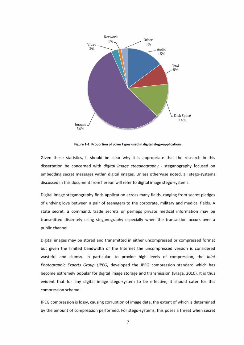
(Johnson & Sallee, 2008), is shown in Figure 1-1.
7
Figure 1-1. Proportion of cover types used in digital stego-applications
Given these statistics, it should be clear why it is appropriate that the research in this
dissertation be concerned with digital image steganography - steganography focused on
embedding secret messages within digital images. Unless otherwise noted, all stego-systems
discussed in this document from hereon will refer to digital image stego-systems.
Digital image steganography finds application across many fields, ranging from secret pledges
of undying love between a pair of teenagers to the corporate, military and medical fields. A
state secret, a command, trade secrets or perhaps private medical information may be
transmitted discretely using steganography especially when the transaction occurs over a
public channel.
Digital images may be stored and transmitted in either uncompressed or compressed format
but given the limited bandwidth of the Internet the uncompressed version is considered
wasteful and clumsy. In particular, to provide high levels of compression, the Joint
Photographic Experts Group (JPEG) developed the JPEG compression standard which has
become extremely popular for digital image storage and transmission (Braga, 2010). It is thus
evident that for any digital image stego-system to be effective, it should cater for this
compression scheme.
JPEG compression is lossy, causing corruption of image data, the extent of which is determined
by the amount of compression performed. For stego-systems, this poses a threat when secret
Audio 15%
Text 8%
Disk Space 14%
Images 56%
Video 3%
Network 1% Other
3%
Sales
8
data is embedded into the image prior to compression and thus requires implementation of
error correcting codes to compensate for the inevitable data corruption. Unfortunately, this
has a negative effect on embedding capacity because error correcting schemes require
transmission of redundant overhead bits (that take up space in an image that could be used for
secret data) that will be used at the receiver to detect and correct erroneous bits.
A type of stego-system that embeds into digital images and tends to accommodate JPEG
compression, called cell-based systems, has emerged as particularly secure. These systems
confuse blind steganalysers by randomising the areas of the image into which data is
embedded. However, as only select areas of the image are used when combined with the
requirement for error coding means that the embedding capacity for these systems is
comparatively low. However, the data embedding and error correcting schemes used in cell-
based systems have not been determined analytically in the literature thus far, and so this
research addresses the extent to which these schemes can be chosen more methodically so
that embedding capacity is improved while maintaining good security properties.
1.5 Research Problem Statement
With relevant background regarding digital image steganography explained, the main purpose
of this research can now be stated.
Given the relevance of cell-based systems in modern digital image steganography, the main
issue addressed in this dissertation is how to develop an approach to analytically determine
data handling (i.e. data embedding and error coding) schemes for cell-based stego-systems so
that embedding capacity is improved and security properties are maintained. This approach
should give rise to a set of data handling parameters that can then be implemented in the
context of cell-based systems and tested for performance.
1.6 Research Methodology
In order to address the research problem statement, certain steps need to be taken. The
research methodology refers to the logical sequence of actions required to gather sufficient
knowledge to address the research problem statement and to test the results. The
methodology can be broken down into the following four stages:
1. The first stage requires background research to develop an understanding of the field of
digital image steganography, including the general philosophies behind design, generic
system models and terminology. In the process, an understanding of the context within
which cell-based systems were developed and their purpose is acquired.

9
2. The second stage requires analysis of cell-based systems and identification of potential
areas of improvement in terms of data embedding and error correction.
3. The third stage requires implementation of a simulator to re-enact cell-based systems and
to analyse the extent to which improvements can be made. This results in the proposition
of new data embedding and error coding schemes.
4. In the final stage, the new data handling schemes are placed back into context and are used
within cell-based systems that are then tested for security and the extent to which
embedding capacity has been improved.
1.7 Dissertation Roadmap
Chapter 2 presents a model of the digital image steganographic systems considered in this
dissertation along with relevant terminology and system characteristics. The development of
digital image stego-systems is then traced, which provides the context within which cell-based
systems were developed. The operational steps of cell-based systems and their varieties are
then presented.
Chapter 3 introduces a new approach to embedding data and correcting errors in cell-based
systems, based primarily on accommodating the effects of lossy JPEG compression. This
approach is explored further and data handling parameters are derived.
Chapter 4 tests the new data embedding and error coding systems with respect to security,
embedding rate and error rate requirements.
Chapter 5 summarises the main points of the dissertation and discusses the extent to which
the original goals presented in this chapter are addressed. Some suggestions for future work
that could build on this research are provided.
1.8 Published Works
The published works based on the research described in the dissertation are:
1. Optimising the Error-Free Embedding Rate in Variable Cell-Size Steganographic Schemes
at the Military Information and Communications Symposium of South Africa (MICSSA)
2011
2. Quantifying Steganographic Embedding Capacity in DCT-Based Embedding Schemes at the
Southern African Telecommunication Networks and Applications Conference (SATNAC)
2011

10
Chapter 2. Digital Image Steganographic Systems
So far, the relevance of digital image steganography as a field of research given the
predominance of digital image exchanges on the Internet has been discussed. These digital
images can be stored in compressed or uncompressed formats but given bandwidth limitations
on channels over the Internet plus the significant volume of storage required for the huge
number of images, compressed formats are more useful and thus popular and in particular
JPEG compression is extremely common.
Within digital image steganographic systems, cell-based systems have emerged as particularly
secure and are designed to cater for the likely application of JPEG compression but
unfortunately display relatively low embedding capacity properties. However, data embedding
and error coding systems have not been determined analytically in the literature thus far, and
so there is an opportunity to improve embedding capacity of cell-based systems by
determining more effective data handling procedures. This idea forms the foundation for this
research which aims to develop an approach to doing this.
Before this approach is developed specifically, this chapter formally defines the relevant
properties of digital image steganographic systems, contextualises and motivates cell-based
systems within digital image steganography and discusses cell-based systems as they are
currently presented in the literature.
2.1 Classification of Steganographic Systems
Many varieties of stego-systems exist and the nature of the systems referred to in this
dissertation is now clarified. Stego-systems may be broadly classified according to
dependencies between the secret data and cover image, the role of the key and the behaviour
of the warden.
2.1.1 Relationship between Secret Message and Cover Image
In the first broad category, stego-systems vary according to the relationship between the
secret message and the image into which it is hidden. As presented by (Fridrich J. , 2010), there
are three main types of stego-systems based on this:
Steganography by cover selection
Alice has access to a fixed database of images, and she chooses the one that communicates
the required message based on some features such as a certain sequence of colours. This
has the disadvantage that Alice may have difficulty finding an appropriate image.
11
Steganography by cover synthesis
Alice creates a cover so that it conveys the required message. She can do this, for example,
by placing certain objects in the frame of a photograph which she then uses as the cover
image. However, this is clumsy and difficult for Alice, who needs to keep setting up frames
and taking photos.
Steganography by cover modification
Alice starts with any cover image and embeds data into it by modifying it according to some
protocol. This type of stego-system is the most practical for communicating large amounts
of data out of the three categories listed here because Alice can theoretically select any
image as a cover. This is the most studied steganographic paradigm.
Since steganography by cover modification is, by far, the most favoured by the research
community, this form of steganography is assumed here.
2.1.2 Key Type
The concept of a key was mentioned in Chapter 1 as something shared between the sender
and intended recipient only and which provides the specifics of the way in which data is
embedded for a particular transaction. For example, in the case of Jane sending her friend
Kevin an email arranging a meeting time as in Chapter 1, the stego-system is the embedding of
one sentence into another but the key specifies which letters in the transmitted sentence
should be extracted to reveal the message. In the example provided, the key for that specific
transaction indicated to Kevin to extract the second letter of each word.
In the prisoners’ problem, it is assumed that Eve knows the complete steganographic
algorithm used by Alice and Bob with the exception of the transaction-specific key which was
agreed upon by the prisoners before imprisonment. The expectation that the stego-algorithm
but not the stego-key be known to Eve is called Kerckhoffs’ principle which states that security
should be maintained not by the secrecy of the system but be based on the key. First
articulated in 1883 (Kerckhoffs, 1883), it stems from experience through espionage where the
stego-algorithm was usually discovered by the enemy. In this event, the security of the stego-
system should not be threatened.
12
The varying role and nature of the key was first used to classify stego-systems in (Anderson R. ,
1996). The given system categories are:
Pure systems
No key is used. Once the stego-system itself is known, the hidden message can be
extracted. This system does not follow Kerckhoffs’ principle and is considered poor.
Secret-key (Symmetric) systems
The same key is used to both embed and extract the hidden information from the image
and it is assumed that this key is secretly shared between the sender and intended
recipient.
Public-key (Asymmetric) systems
These systems use two keys – a public key that is openly published and a private key known
only to the intended recipient. The information is embedded using a public key and
extracted using the private key. Contrary to secret-key systems, these systems exhibit
asymmetry in that the key used to embed information in the image is not the same one
used to extract that secret information.
Secret-key systems are the most popular in the literature, and this type of system will be
assumed in this dissertation.
2.1.3 Role of the Warden
The possibilities of warden behaviour were already described in Chapter 1 as passive, active or
malicious. Steganalysis was defined as the science of distinguishing between innocent and
corrupt digital images in the case of the passive warden scenario which is by far the most
common paradigm in the literature on digital image steganography and hence the passive
warden scenario is the assumed model for this work.
2.2 Stego-System Model
A formal stego-system model is shown in Figure 2-1. Figure 2-1 and the terminology explained
in this section were agreed upon at the first international workshop on information hiding
((Anderson R. , 1996), (Pfitzmann & Anderson, 1996)).

13
Figure 2-1. Overview of stego-system
Steganography is used when there is a need to transmit a secret message which is achieved by
hiding it in a cover image. It is important that the innocent cover image itself is not publicly
available, as this would make steganalysis by the warden a trivial exercise of comparison
between a suspect stego-image and its innocent version.
The message is any data represented by a bit stream. In binary digital communications, all
information is ultimately represented in bits so there is no requirement that the cover and
message objects have the same original form (e.g. audio, video, text). The process with which
the message is embedded in its cover is called the embedding algorithm, the result of which is
called a stego-image.
Mathematically, the embedding algorithm can be expressed as shown in Equation 2-1.
2-1
where is the stego-object, is the cover object, is the secret-key and is the secret
message.
The stego-image is then transmitted across an unsecured, public channel which we assume is
error-free (passive warden scenario). If the stego-image is compressed, the compressed
version is sent over the channel and may undergo steganalysis.
Cover (Carrier) object
Stego-key Secret Message
(Embedded Data)
Embedding Algorithm
Stego-object Transmit over public channel
Stego-object Stego-key
Secret Message (Embedded Data)
Transmit over secret channel
Extraction Algorithm
14
At the receiver side, the secret message is retrieved using the stego-key and an extraction
algorithm, shown in Equation 2-2.
2-2
The embedding and extraction algorithms may be designed specifically so that the original
cover image can be retrieved by the recipient in what is called a lossless data hiding scheme.
This is not relevant here because the cover image itself is not considered to have any value. A
lossless scheme would be more relevant in a watermarking application.
2.3 Pertinent Properties of Stego-Systems
Now that the structure and relevant terminology relating to stego-systems has been described,
the next relevant concept is that of performance of stego-systems. The requirement for
security against steganalysis has already been mentioned and this section describes two other
important performance requirements. It also describes in more detail what is meant by
security and resistance to steganalysis.
2.3.1 Primary Attributes
(Smith & Comiskey, 1996) define three primary attributes for an information hiding system;
imperceptibility, embedding capacity and robustness:
Imperceptibility
The difficulty a warden has in detecting the presence of hidden information or, more
specifically, the uncertainty with which a warden can classify corrupt stego-images from
innocent cover images. This has already been mentioned under the description of
steganalysis.
Embedding Capacity
Sometimes referred to as effective payload or simply capacity, it is the amount of
information (excluding any overhead or dummy bits) that can be hidden in a given cover
image. The larger the capacity of a stego-system, the better the system.
Robustness
The amount of modification the stego-image can undergo before the hidden information
becomes irretrievably damaged. Depending on whether the stego-object is likely to
undergo alteration this may or may not be a critical attribute.
15
There is general agreement in the literature that imperceptibility and capacity are the most
important of the attributes (e.g. (Luo, Huang, & Huang, 2010), (Smith & Comiskey, 1996)). In
other words, a good stego-system should embed as much data as possible and keep distortion
as low as possible. It should only be robust when the application requires it. Furthermore, a
system is effectively useless if it does not effectively combat steganalytic attacks, no matter
how robust or how much capacity it has.
The three properties contradict one another and thus it is impossible to achieve a system that
has all three excellent qualities. For example, if the amount of hidden information is increased
(i.e. increased capacity), the warden will have more chance of detecting it (i.e. lower
imperceptibility) since inevitably more artefacts indicating embedding will be introduced into
the cover.
In order to maintain imperceptibility, the stego-system should firstly not introduce any obvious
visual artefacts into the stego-image during embedding. The visual imperceptibility associated
with a stego-image is often measured in the literature using the mean square error (MSE) or
peak signal to noise ratio (PSNR) that is calculated as the average difference in colours
between the innocent cover image and stego-image. However, these measures offer only a
limited reflection of imperceptibility. To demonstrate this, consider the two images of Lena
shown in Figure 2-2.
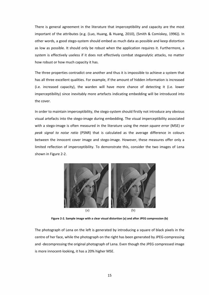
Figure 2-2. Sample image with a clear visual distortion (a) and after JPEG compression (b)
The photograph of Lena on the left is generated by introducing a square of black pixels in the
centre of her face, while the photograph on the right has been generated by JPEG-compressing
and -decompressing the original photograph of Lena. Even though the JPEG compressed image
is more innocent-looking, it has a 20% higher MSE.
(a) (b)
16
The main problem with the MSE is that it measures the average difference between the
colours of the stego-image and cover image, and so localised distortion on a small scale, even
if clearly visible, is not represented. Unfortunately, as it shall be seen, papers on the topic of
digital image steganography still use the MSE as a measure of performance. A more useful
measure of visual perceptibility would be the success of human suspects categorising innocent
and corrupt images visually as done in (Dawoud, 2010).
One additional property of a stego-system apart from the three discussed that merits
mentioning is the computational demand in implementing it (Fan & Wediong, 2004). Generally
the more complex the embedding scheme, the more secure the system. However, the
processing power of modern, commercially-available computers more than suffices for any
requirements, even in the most complex of schemes, especially since there are no
requirements for ultra-fast real-time implementation. Restrictions in system complexity arise
when the scheme is limited to embedded devices as seen in (Stanescu, Stangaciu, & Stratulat,
2010). These types of limitations and applications are not assumed here, so simplicity in
algorithm and execution time is not used as a measure of success of a system.
2.3.2 Detectability versus Imperceptibility
Given that most images transmitted over the Internet are displayed at some point if not
directly uploaded to a public website, it would be foolish for a stego-system to introduce
obvious visual distortion to a stego-image since this would immediately arouse suspicion. Over
time the complexity of both steganographic and steganalytic techniques has increased,
primarily in response to each other’s development in a spiral development pattern. The
requirement of visual imperceptibility is no longer sufficient in itself and the combat between
data hiding and the attack has moved to a more subtle, statistical level. Modern steganalytic
techniques classify images based on changes and boundaries in statistics across an image
rather than any visual artefacts (Fridrich & Goljan, 2002). No matter how imperceptible the
embedding artefacts visually, appreciable statistical traces of embedding in an image may
usually be determined.
At this point an extra attribute is introduced - detectability which is used to refer to the extent
to which steganalytic techniques detect stego-images through statistical means whereas
perceptibility is now re-defined to be limited to the extent to which embedding artefacts are
visually clear. Visual embedding artefacts will automatically introduce statistical anomalies
(but not vice-versa) therefore a system that is undetectable will also be imperceptible but the
opposite is not true. In this dissertation, the term naïve will be used to refer to old-fashioned
17
stego-systems that aim for imperceptibility only and complex will be used for modern stego-
schemes that aim to avoid detectability.
Generally, the similarity between an innocent cover image and stego-image (visually or
otherwise) may be expressed using a property called Transparency (where is the cover
object and the stego-image):
2-3
In the case of a secure system, Equation 2-3 can be re-written as shown in Equation 2-4.
( ( )) 2-4
A stego-system is secure if a warden can only guess whether an image is corrupt or innocent
and equally determines stego-images as innocent and innocent images as stego-images. This
can be stated differently as that the warden achieves a detection rate of 0.5.
There are more formal definitions of security and one popular definition by Cahin (Cahin,
2004) uses information theory to compare the distribution of innocent cover objects and
stego-objects. His definition is given next.
By first defining:
... Set of cover object
..Set of stego-object for
... Set of stego-keys for
... Set of all messages that can be communicated in .
Equations 2-1 and 2-2 can be rewritten as shown in Equations 2-5 and 2-6.
2-5
2-6
If we observe the transactions between Alice and Bob for long enough, the images chosen as
covers would produce a probability distribution in the space of all the covers . The
distribution represents legitimate communication between the two. If Alice and Bob now
18
embed secret information in the images (i.e. use the images to generate stego-images), if you
again observe the transactions over a long enough period of time, the images will follow a
different distribution over . Intuitively, the stego-system should be designed so that is
as close as possible to . If and are similar, the warden will make erroneous decisions
more often. The two distributions can be compared using the KL distance or relative entropy,
which is a fundamental concept from information theory for measuring the difference
between distributions, given in Equation 2-7.
∑
2-7
A completely secure stego-system is one where the distribution of the resultant stego-objects
exactly follows that of innocent cover objects so that the warden cannot distinguish between
the two distributions. In this case , and the KL distance is zero. This means that no
steganalytic scheme can perform better than a random guess.
If we write:
2-8
Then we say that the system is ε-secure. Through calculations not detailed here but available in
(Fridrich J. , 2010), this translates to the fact that if we assume that the warden is not allowed
to falsely accuse the prisoners, the smaller the value of ε, the lower the probability of
detection. This motivates the use of the KL divergence as a measure of the security of the
stego-system.
It is convenient to use KL divergence for comparing two systems. For example, if you have two
systems S(1) and S(2), we would say S(1) is more secure that S(2) if:
( ) (
) 2-9
2.4 Taxonomy of Digital Image Steganography
The development of digital image steganographic systems has been fuelled mainly by advances
in steganalytic methods for detecting ever more subtle statistical embedding artefacts. Data
hiding in the spatial, uncompressed representation of digital images came first followed by the
idea of transform-based data hiding. The development of stego-systems from naïve to complex
and the context within which cell-based systems were developed is explained in this section.
Cell-based systems are then described as they are currently defined in the literature.
19
2.4.1 Spatial Domain Steganography
The first naïve digital image stego-systems focused on embedding data bits in the spatial
domain representation of images with the purpose of avoiding perceptible artefacts. Initially,
the idea of transform representation and image compression were not known or referred to.
This section explains the spatial domain representation of images and then how spatial stego-
systems were designed to operate.
2.4.1.1 Spatial Domain Representation
The spatial domain representation of an image deals with representing the colours of a real-
world scene in digital format. Visible light consists of the sum of electromagnetic waves with
wavelengths between approximately 280nm and 750nm. A colour is defined by a combination
of waves, each one of a particular wavelength and energy. Even though there are infinitely
many different colours in the real world, the human eye is capable of distinguishing only a
small subset of them.
When digital cameras capture a scene, they must digitise the light information in the frame
before storage, the result of which is the digital image. Spatially, a digital image may be
defined as a discrete 2-dimensional function where and are spatial coordinates and
the value of at point is called the intensity of that point. Each point in the image is
called a pixel.
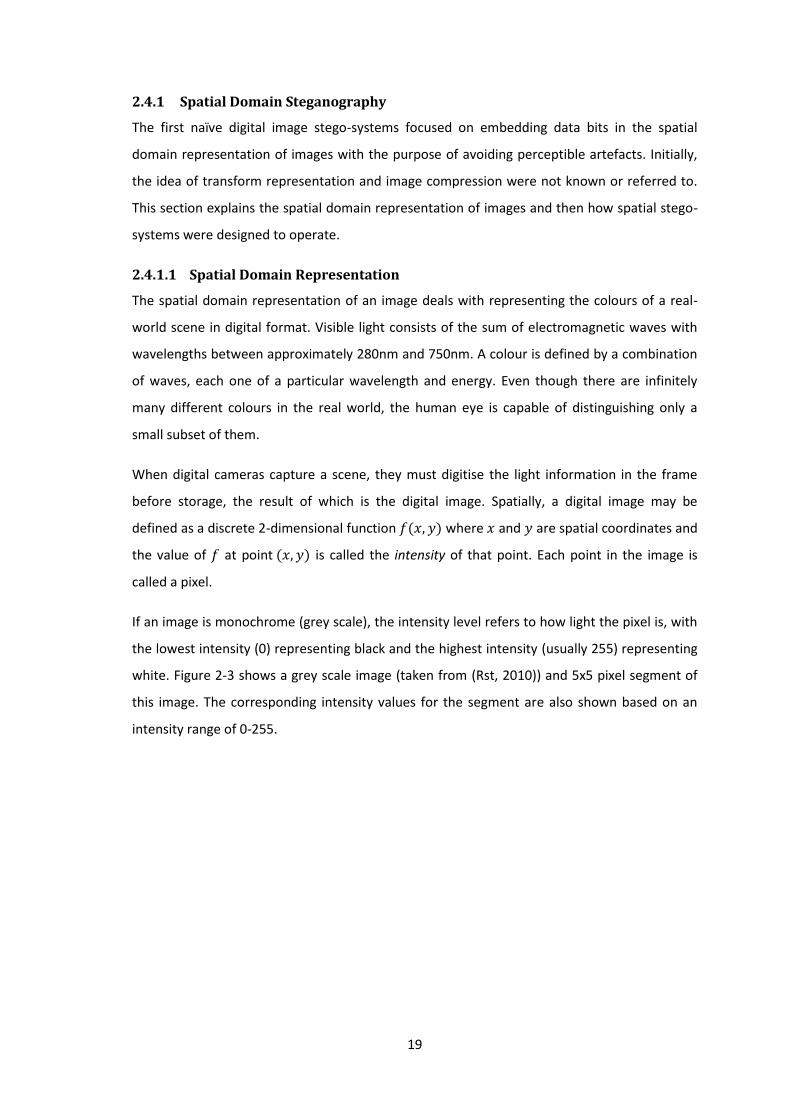
If an image is monochrome (grey scale), the intensity level refers to how light the pixel is, with
the lowest intensity (0) representing black and the highest intensity (usually 255) representing
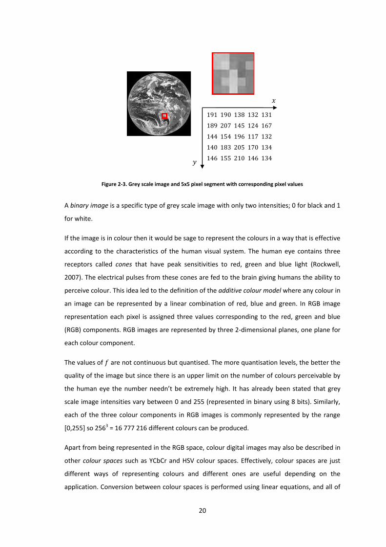
white. Figure 2-3 shows a grey scale image (taken from (Rst, 2010)) and 5x5 pixel segment of
this image. The corresponding intensity values for the segment are also shown based on an
intensity range of 0-255.
20
Figure 2-3. Grey scale image and 5x5 pixel segment with corresponding pixel values
A binary image is a specific type of grey scale image with only two intensities; 0 for black and 1
for white.
If the image is in colour then it would be sage to represent the colours in a way that is effective
according to the characteristics of the human visual system. The human eye contains three
receptors called cones that have peak sensitivities to red, green and blue light (Rockwell,
2007). The electrical pulses from these cones are fed to the brain giving humans the ability to
perceive colour. This idea led to the definition of the additive colour model where any colour in
an image can be represented by a linear combination of red, blue and green. In RGB image
representation each pixel is assigned three values corresponding to the red, green and blue
(RGB) components. RGB images are represented by three 2-dimensional planes, one plane for
each colour component.
The values of are not continuous but quantised. The more quantisation levels, the better the
quality of the image but since there is an upper limit on the number of colours perceivable by
the human eye the number needn’t be extremely high. It has already been stated that grey
scale image intensities vary between 0 and 255 (represented in binary using 8 bits). Similarly,
each of the three colour components in RGB images is commonly represented by the range
[0,255] so 2563 = 16 777 216 different colours can be produced.
Apart from being represented in the RGB space, colour digital images may also be described in
other colour spaces such as YCbCr and HSV colour spaces. Effectively, colour spaces are just
different ways of representing colours and different ones are useful depending on the
application. Conversion between colour spaces is performed using linear equations, and all of
191 190 138 132 131
189 207 145 124 167
144 154 196 117 132
140 183 205 170 134
146 155 210 146 134
𝑥
𝑦
21
them can be derived from the RGB space. The conversion between RGB space and YCbCr (Y
meaning luminance and (CbCr) meaning chrominance) space, for example, is given in Equation
2-10 (Gonzalez & Woods, Image Types, 2002).
[
] [
] [
] [ ] 2-10
Images represented in the manner explained so far are called intensity images.
Images may also be represented as indexed images. In this format, the image is represented by
a data matrix of integers and an associated colour map matrix. The values associated with each
pixel act as pointers directly to colours in the map. Indexed images were used to save space by
representing each RGB pixel by an 8 bit index into a colour table. The resultant images were of
a lower quality than a full colour image and as storage space has become less critical, indexed
images have lost favour and are very seldom used anymore. In this dissertation, only RGB and
YCbCr images will be used.
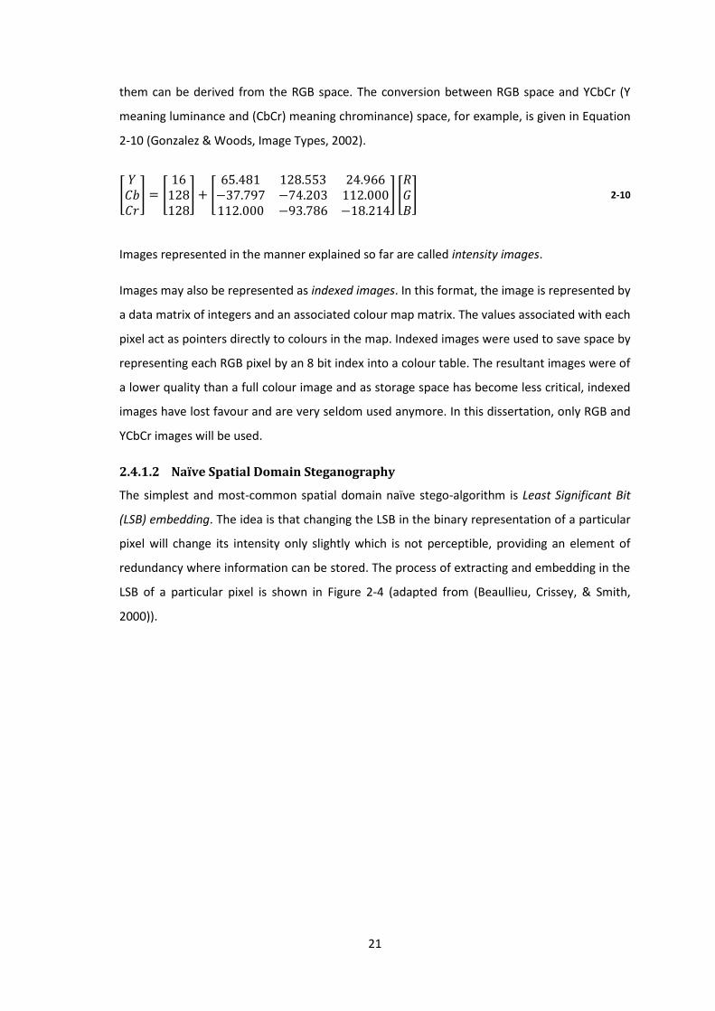
2.4.1.2 Naïve Spatial Domain Steganography
The simplest and most-common spatial domain naïve stego-algorithm is Least Significant Bit
(LSB) embedding. The idea is that changing the LSB in the binary representation of a particular
pixel will change its intensity only slightly which is not perceptible, providing an element of
redundancy where information can be stored. The process of extracting and embedding in the
LSB of a particular pixel is shown in Figure 2-4 (adapted from (Beaullieu, Crissey, & Smith,
2000)).
22
Figure 2-4. LSB embedding
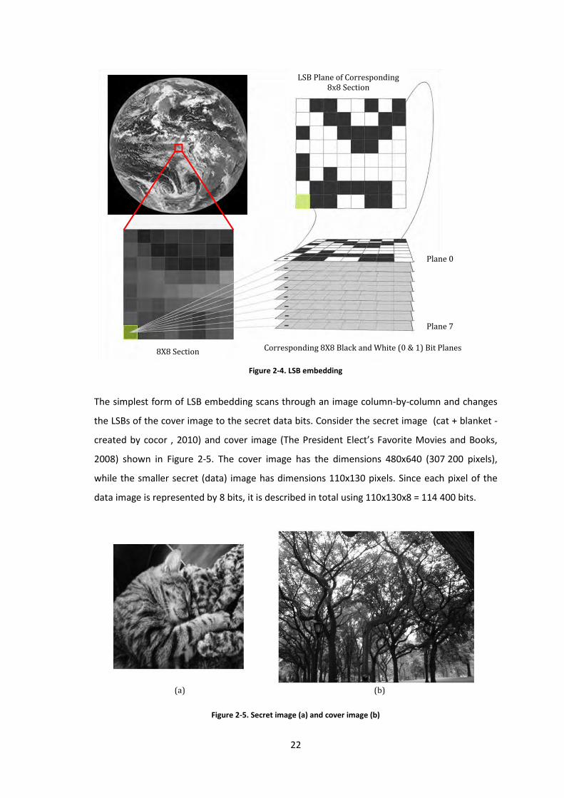
The simplest form of LSB embedding scans through an image column-by-column and changes
the LSBs of the cover image to the secret data bits. Consider the secret image (cat + blanket -
created by cocor , 2010) and cover image (The President Elect’s Favorite Movies and Books,
2008) shown in Figure 2-5. The cover image has the dimensions 480x640 (307 200 pixels),
while the smaller secret (data) image has dimensions 110x130 pixels. Since each pixel of the
data image is represented by 8 bits, it is described in total using 110x130x8 = 114 400 bits.
Figure 2-5. Secret image (a) and cover image (b)
8X8 Section
LSB Plane of Corresponding 8x8 Section
Plane 0
Plane 7
Corresponding 8X8 Black and White (0 & 1) Bit Planes
(b) (a)
23
If each bit of the secret image is embedded into the LSB of a pixel in the cover image, the
secret image fits into a small section of the cover image. If the image is traversed column-by-
column, the resultant stego-image is shown in Figure 2-6.
Figure 2-6. Stego-image using LSB embedding with a small secret message
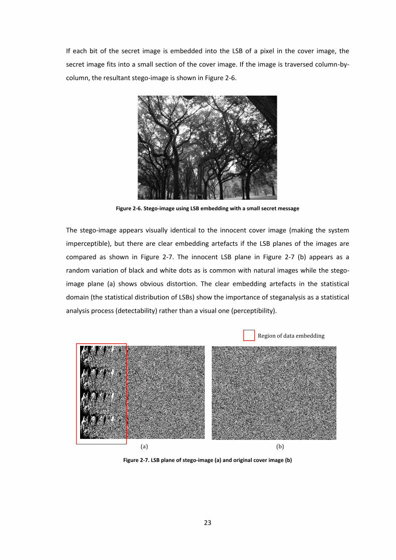
The stego-image appears visually identical to the innocent cover image (making the system
imperceptible), but there are clear embedding artefacts if the LSB planes of the images are
compared as shown in Figure 2-7. The innocent LSB plane in Figure 2-7 (b) appears as a
random variation of black and white dots as is common with natural images while the stego-
image plane (a) shows obvious distortion. The clear embedding artefacts in the statistical
domain (the statistical distribution of LSBs) show the importance of steganalysis as a statistical
analysis process (detectability) rather than a visual one (perceptibility).
Figure 2-7. LSB plane of stego-image (a) and original cover image (b)
Region of data embedding
(a) (b)
24
Apart from its high detectability, performing LSB embedding column-by-column has the
disadvantage that a key is not required in disagreement with Kerckhoffs’ principle, making it a
poor system.
An improvement would be to use a pseudo-random number generator (PRNG) to distribute
the LSB changes throughout the image spreading the artefacts over the entire plane and
making them less obvious. The system now also follows Kerckhoffs’ principle since the receiver
would not know the path with which data was embedded without the key to the PRNG.
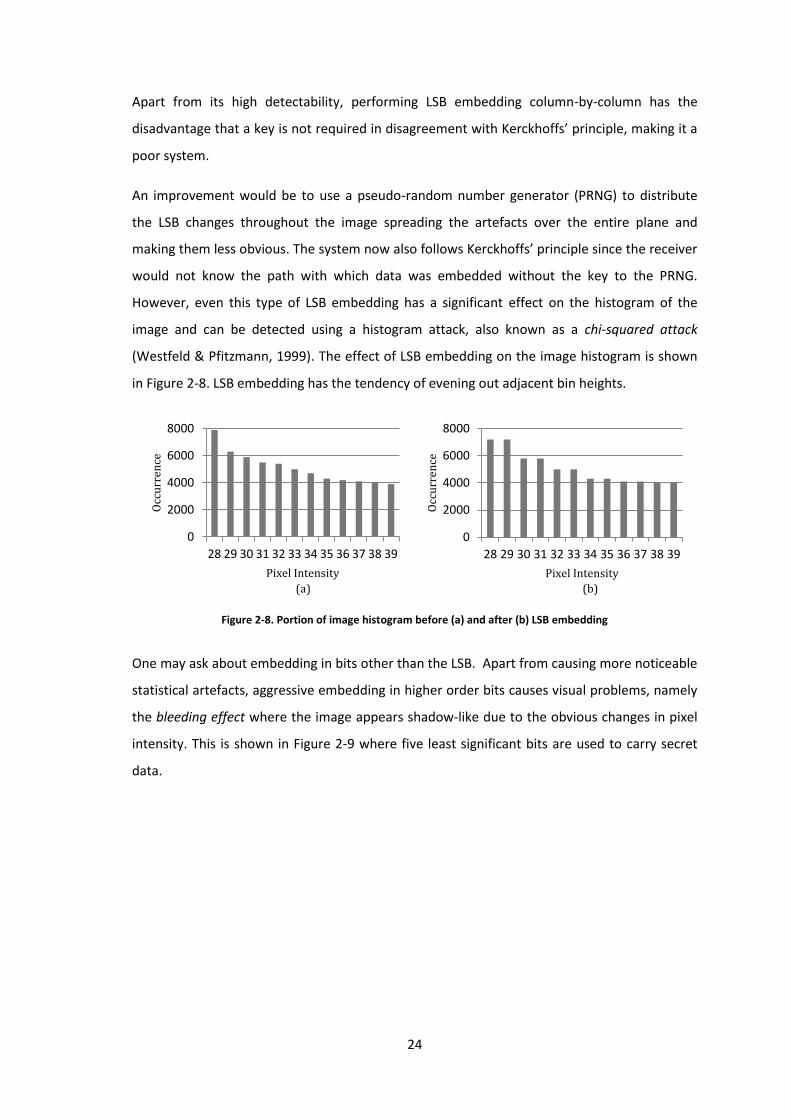
However, even this type of LSB embedding has a significant effect on the histogram of the
image and can be detected using a histogram attack, also known as a chi-squared attack
(Westfeld & Pfitzmann, 1999). The effect of LSB embedding on the image histogram is shown
in Figure 2-8. LSB embedding has the tendency of evening out adjacent bin heights.
Figure 2-8. Portion of image histogram before (a) and after (b) LSB embedding
One may ask about embedding in bits other than the LSB. Apart from causing more noticeable
statistical artefacts, aggressive embedding in higher order bits causes visual problems, namely
the bleeding effect where the image appears shadow-like due to the obvious changes in pixel
intensity. This is shown in Figure 2-9 where five least significant bits are used to carry secret
data.
0
2000
4000
6000
8000
28 29 30 31 32 33 34 35 36 37 38 39
Occ
urr
ence
Pixel Intensity
0
2000
4000
6000
8000
28 29 30 31 32 33 34 35 36 37 38 39
Occ
urr
ence
Pixel Intensity
(a) (b)
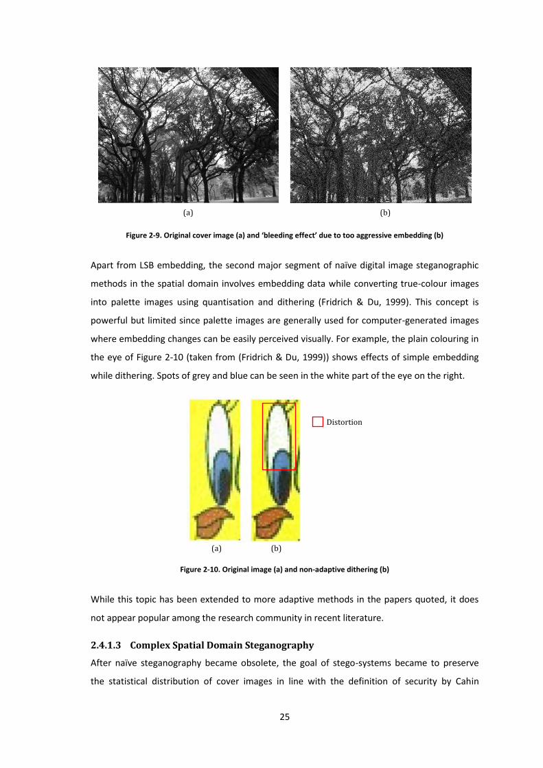
25
Figure 2-9. Original cover image (a) and ‘bleeding effect’ due to too aggressive embedding (b)
Apart from LSB embedding, the second major segment of naïve digital image steganographic
methods in the spatial domain involves embedding data while converting true-colour images
into palette images using quantisation and dithering (Fridrich & Du, 1999). This concept is
powerful but limited since palette images are generally used for computer-generated images
where embedding changes can be easily perceived visually. For example, the plain colouring in
the eye of Figure 2-10 (taken from (Fridrich & Du, 1999)) shows effects of simple embedding
while dithering. Spots of grey and blue can be seen in the white part of the eye on the right.
Figure 2-10. Original image (a) and non-adaptive dithering (b)
While this topic has been extended to more adaptive methods in the papers quoted, it does
not appear popular among the research community in recent literature.
2.4.1.3 Complex Spatial Domain Steganography
After naïve steganography became obsolete, the goal of stego-systems became to preserve
the statistical distribution of cover images in line with the definition of security by Cahin
(a) (b)
(a) (b)
Distortion
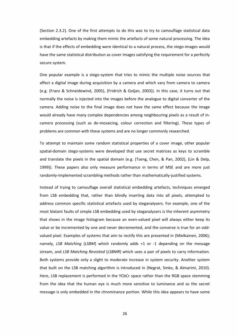
26
(Section 2.3.2). One of the first attempts to do this was to try to camouflage statistical data
embedding artefacts by making them mimic the artefacts of some natural processing. The idea
is that if the effects of embedding were identical to a natural process, the stego-images would
have the same statistical distribution as cover images satisfying the requirement for a perfectly
secure system.
One popular example is a stego-system that tries to mimic the multiple noise sources that
affect a digital image during acquisition by a camera and which vary from camera to camera
(e.g. (Franz & Schneidewind, 2005), (Fridrich & Goljan, 2003)). In this case, it turns out that
normally the noise is injected into the images before the analogue to digital converter of the
camera. Adding noise to the final image does not have the same effect because the image
would already have many complex dependencies among neighbouring pixels as a result of in-
camera processing (such as de-mosaicing, colour correction and filtering). These types of
problems are common with these systems and are no longer commonly researched.
To attempt to maintain some random statistical properties of a cover image, other popular
spatial-domain stego-systems were developed that use secret matrices as keys to scramble
and translate the pixels in the spatial domain (e.g. (Tseng, Chen, & Pan, 2002), (Lin & Delp,
1999)). These papers also only measure performance in terms of MSE and are more just
randomly-implemented scrambling methods rather than mathematically-justified systems.
Instead of trying to camouflage overall statistical embedding artefacts, techniques emerged
from LSB embedding that, rather than blindly inserting data into all pixels, attempted to
address common specific statistical artefacts used by steganalysers. For example, one of the
most blatant faults of simple LSB embedding used by steganalysers is the inherent asymmetry
that shows in the image histogram because an even-valued pixel will always either keep its
value or be incremented by one and never decremented, and the converse is true for an odd-
valued pixel. Examples of systems that aim to rectify this are presented in (Mielkainen, 2006);
namely, LSB Matching (LSBM) which randomly adds +1 or -1 depending on the message
stream, and LSB Matching Revisited (LSBMR) which uses a pair of pixels to carry information.
Both systems provide only a slight to moderate increase in system security. Another system
that built on the LSB matching algorithm is introduced in (Negrat, Smko, & Almarimi, 2010).
Here, LSB replacement is performed in the YCbCr space rather than the RGB space stemming
from the idea that the human eye is much more sensitive to luminance and so the secret
message is only embedded in the chrominance portion. While this idea appears to have some
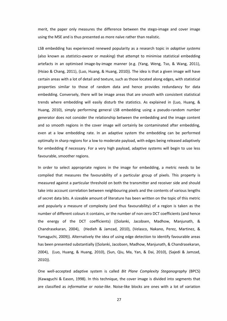
27
merit, the paper only measures the difference between the stego-image and cover image
using the MSE and is thus presented as more naïve rather than realistic.
LSB embedding has experienced renewed popularity as a research topic in adaptive systems
(also known as statistics-aware or masking) that attempt to minimise statistical embedding
artefacts in an optimised image-by-image manner (e.g. (Yang, Weng, Tso, & Wang, 2011),
(Hsiao & Chang, 2011), (Luo, Huang, & Huang, 2010)). The idea is that a given image will have
certain areas with a lot of detail and texture, such as those located along edges, with statistical
properties similar to those of random data and hence provides redundancy for data
embedding. Conversely, there will be image areas that are smooth with consistent statistical
trends where embedding will easily disturb the statistics. As explained in (Luo, Huang, &
Huang, 2010), simply performing general LSB embedding using a pseudo-random number
generator does not consider the relationship between the embedding and the image content
and so smooth regions in the cover image will certainly be contaminated after embedding,
even at a low embedding rate. In an adaptive system the embedding can be performed
optimally in sharp regions for a low to moderate payload, with edges being released adaptively
for embedding if necessary. For a very high payload, adaptive systems will begin to use less
favourable, smoother regions.
In order to select appropriate regions in the image for embedding, a metric needs to be
compiled that measures the favourability of a particular group of pixels. This property is
measured against a particular threshold on both the transmitter and receiver side and should
take into account correlation between neighbouring pixels and the contents of various lengths
of secret data bits. A sizeable amount of literature has been written on the topic of this metric
and popularly a measure of complexity (and thus favourability) of a region is taken as the
number of different colours it contains, or the number of non-zero DCT coefficients (and hence
the energy of the DCT coefficients) ((Solanki, Jacobsen, Madhow, Manjunath, &
Chandrasekaran, 2004), (Hedieh & Jamzad, 2010), (Velasco, Nakano, Perez, Martinez, &
Yamaguchi, 2009)). Alternatively the idea of using edge detection to identify favourable areas
has been presented substantially ((Solanki, Jacobsen, Madhow, Manjunath, & Chandrasekaran,
2004), (Luo, Huang, & Huang, 2010), (Sun, Qiu, Ma, Yan, & Dai, 2010), (Sajedi & Jamzad,
2010)).
One well-accepted adaptive system is called Bit Plane Complexity Steganography (BPCS)
(Kawaguchi & Eason, 1998). In this technique, the cover image is divided into segments that
are classified as informative or noise-like. Noise-like blocks are ones with a lot of variation
28
between pixels and are replaced by blocks of secret data. Leading on from this idea, (Kermani
& Jamzad, 2005) replaced similar 4x4 blocks in the cover image with secret blocks. The
problem with this simplistic approach is that it only analyses a particular block/region itself
without looking at surrounding pixels. Therefore, by simply replacing the blocks, virtual edges
and corners appear that present detectable global statistical irregularities. In (Sajedi & Jamzad,
2008) this is addressed by considering block texture and neighbourhood information in the
metric so that there is less distortion. The papers on these topics, however, tend to focus on
minimising the visual distortion and do not test the system performance against steganalysers.
One may wonder how the feature selection criterion for a particular adaptive system is
transmitted to the intended receiver. One possibility is to assume that for a particular
property, the value of that property compared to a set threshold is what decides whether or
not some section of the image is appropriate for embedding. Both the sender and receiver
could use this threshold as a test while embedding and extracting. However, it is not
guaranteed that the property of the segment after embedding will still lie on the same side of
the threshold. Systems assume that this will probably be the case. If not, then the embedded
block is left as is, and the same data is embedded into the next block until the embedded
segment lies on the same side of the threshold (Luo, Huang, & Huang, 2010). An alternative
would be to use what is called wet paper codes, introduced in (Fridrich J. , Goljan, Lisoňek, &
Soukal, 2004) and used in situations where the recipient is not aware of where data was
embedded. In other words, we assume that that the selection rules used by the sender based
on side information is not available to an attacker or the recipient. The metaphor of “writing
on wet paper” is explained by imagining that some water drops have fallen onto a piece of
paper. The sender can only modify the dry regions, but once the paper has dried, the recipient
cannot tell which regions were used by the sender. These codes are valuable because they are
more secure than systems where the selection rules are publicly available. Apart from adaptive
systems, there may be certain areas of a cover image in, for example, sensitive medical or
military applications, which cannot be edited. Wet paper codes use a principle from error-
correcting in digital communications called syndrome coding. The mathematical theory is for
this is not explained here but may be read in (Fridrich J. , Goljan, Lisoňek, & Soukal, 2004).
In addition to adapting the stego-algorithm according to the cover image, it may be useful to
choose, within reason, the most appropriate cover images from a set. Images with low
variation and a low number of colours are poor choices. For example, an image of a cloudless
sky over a plain, snowy landscape would be a particularly poor choice as there is hardly any
natural statistical variation and statistical anomalies due to embedding would be easily
29
introduced. Images that are commonly found on the Internet and other public sources are also
not favourable as covers as the attacker will have the advantage of being able to compare the
stego-object to the original cover object which will inevitably provide the most certain of
steganalysis tests. (Hedieh & Jamzad, 2008) emphasise that the ability of steganographers to
select an appropriate cover image is an advantage associated with steganography (versus
watermarking for example). (Hedieh & Jamzad, 2010) suggest choosing cover images with
maximum contrast from the database and even implementing image pre-processing such as
sharpening and contrast-improvement on the cover image before data embedding to increase
statistical variation. The paper finds that performing pre-processing has an acknowledgeable
effect on security for the same level of embedding with security being measured as the
resistance of stego-images to detection by a selected handful of blind steganalysers.
2.4.2 Transform Domain Steganography
With time, steganalysis tools became more intelligent and ensuring visual imperceptibility was
no longer sufficient to maintain security. In addition to this, image compression became a
likely eventuality for cover images especially if they are transmitted using the Internet.
Transform domain stego-systems embed into the transform domain representation of images
and take both of these factors in account and thus emerged as more relevant than spatial
domain systems. This section describes transform domain image representation and, as a side
note, covers JPEG compression preliminarily before reviewing transform-based stego-systems
as they exist in the literature. The literature review provides a short history and context which
then shows the motivation for the creation of cell-based systems.
2.4.2.1 Transform Domain Representation
Instead of representing digital images spatially, they may be represented in some transform
domain, the most common of these being the frequency domain. This is analogous to a time
domain signal being represented by its constituent frequencies using the Fourier transform.
The most commonly-used image transformation between the spatial and frequency domains is
the 2-dimensional Discrete Cosine Transform (DCT) which is computed over a rectangular
group of pixels.
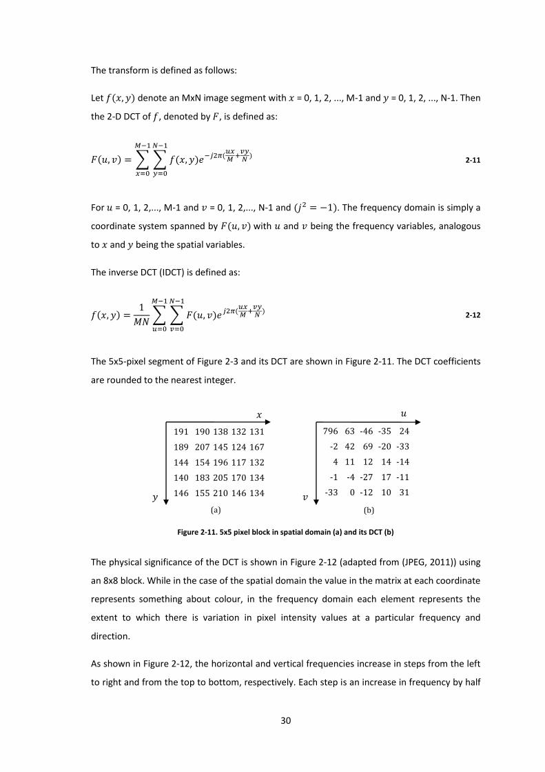
30
The transform is defined as follows:
Let denote an MxN image segment with = 0, 1, 2, ..., M-1 and = 0, 1, 2, ..., N-1. Then
the 2-D DCT of , denoted by , is defined as:
∑ ∑
2-11
For = 0, 1, 2,..., M-1 and = 0, 1, 2,..., N-1 and . The frequency domain is simply a
coordinate system spanned by with and being the frequency variables, analogous
to and being the spatial variables.
The inverse DCT (IDCT) is defined as:
∑ ∑
2-12
The 5x5-pixel segment of Figure 2-3 and its DCT are shown in Figure 2-11. The DCT coefficients
are rounded to the nearest integer.
Figure 2-11. 5x5 pixel block in spatial domain (a) and its DCT (b)
The physical significance of the DCT is shown in Figure 2-12 (adapted from (JPEG, 2011)) using
an 8x8 block. While in the case of the spatial domain the value in the matrix at each coordinate
represents something about colour, in the frequency domain each element represents the
extent to which there is variation in pixel intensity values at a particular frequency and
direction.
As shown in Figure 2-12, the horizontal and vertical frequencies increase in steps from the left
to right and from the top to bottom, respectively. Each step is an increase in frequency by half
191 190 138 132 131
189 207 145 124 167
144 154 196 117 132
140 183 205 170 134
146 155 210 146 134
796 63 -46 -35 24
-2 42 69 -20 -33
4 11 12 14 -14
-1 -4 -27 17 -11
-33 0 -12 10 31
(b) (a)
𝑦
𝑢
𝑣
𝑥
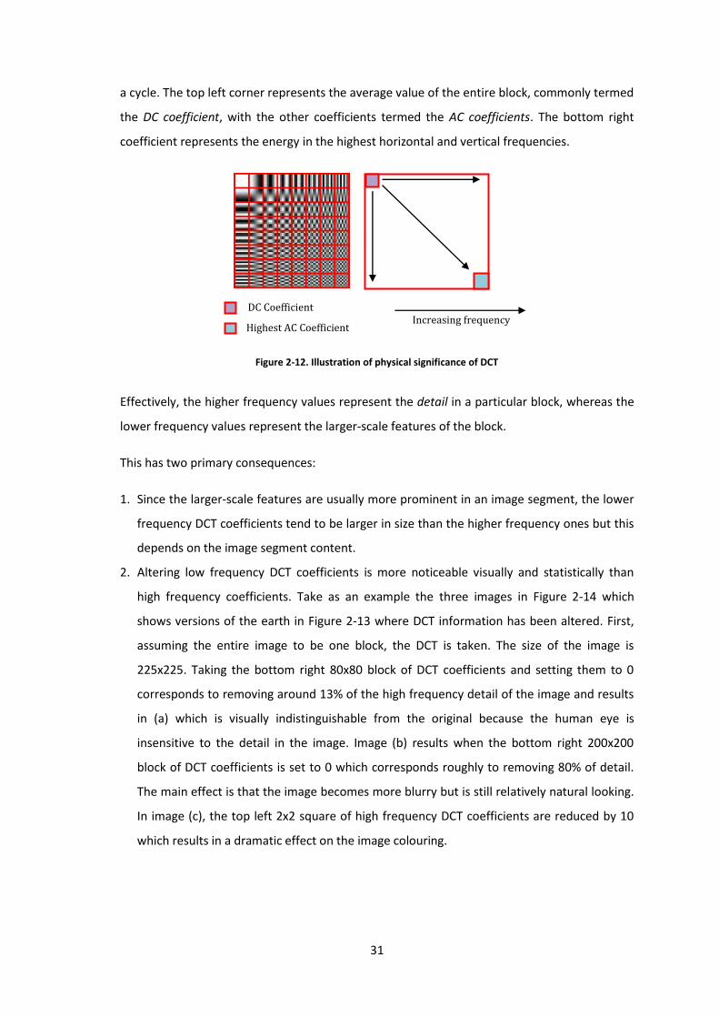
31
a cycle. The top left corner represents the average value of the entire block, commonly termed
the DC coefficient, with the other coefficients termed the AC coefficients. The bottom right
coefficient represents the energy in the highest horizontal and vertical frequencies.
Figure 2-12. Illustration of physical significance of DCT
Effectively, the higher frequency values represent the detail in a particular block, whereas the
lower frequency values represent the larger-scale features of the block.
This has two primary consequences:
1. Since the larger-scale features are usually more prominent in an image segment, the lower
frequency DCT coefficients tend to be larger in size than the higher frequency ones but this
depends on the image segment content.
2. Altering low frequency DCT coefficients is more noticeable visually and statistically than
high frequency coefficients. Take as an example the three images in Figure 2-14 which
shows versions of the earth in Figure 2-13 where DCT information has been altered. First,
assuming the entire image to be one block, the DCT is taken. The size of the image is
225x225. Taking the bottom right 80x80 block of DCT coefficients and setting them to 0
corresponds to removing around 13% of the high frequency detail of the image and results
in (a) which is visually indistinguishable from the original because the human eye is
insensitive to the detail in the image. Image (b) results when the bottom right 200x200
block of DCT coefficients is set to 0 which corresponds roughly to removing 80% of detail.
The main effect is that the image becomes more blurry but is still relatively natural looking.
In image (c), the top left 2x2 square of high frequency DCT coefficients are reduced by 10
which results in a dramatic effect on the image colouring.
DC Coefficient
Highest AC Coefficient Increasing frequency
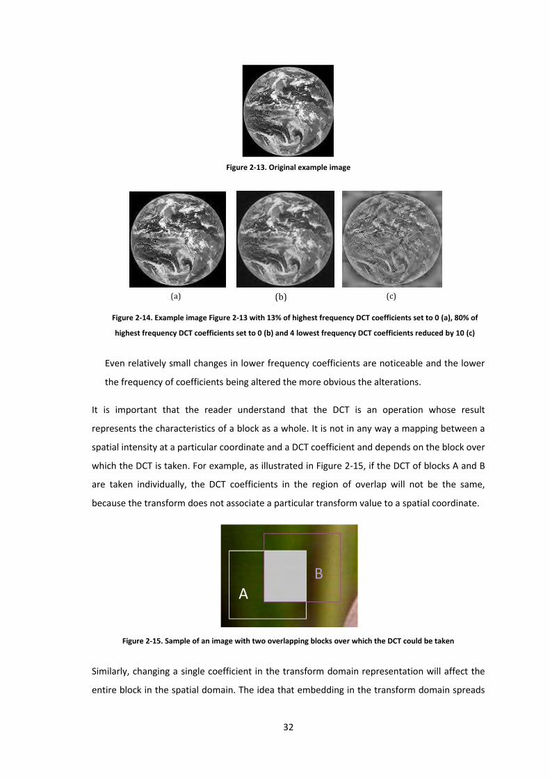
32
Figure 2-13. Original example image
Figure 2-14. Example image Figure 2-13 with 13% of highest frequency DCT coefficients set to 0 (a), 80% of
highest frequency DCT coefficients set to 0 (b) and 4 lowest frequency DCT coefficients reduced by 10 (c)
Even relatively small changes in lower frequency coefficients are noticeable and the lower
the frequency of coefficients being altered the more obvious the alterations.
It is important that the reader understand that the DCT is an operation whose result
represents the characteristics of a block as a whole. It is not in any way a mapping between a
spatial intensity at a particular coordinate and a DCT coefficient and depends on the block over
which the DCT is taken. For example, as illustrated in Figure 2-15, if the DCT of blocks A and B
are taken individually, the DCT coefficients in the region of overlap will not be the same,
because the transform does not associate a particular transform value to a spatial coordinate.
Figure 2-15. Sample of an image with two overlapping blocks over which the DCT could be taken
Similarly, changing a single coefficient in the transform domain representation will affect the
entire block in the spatial domain. The idea that embedding in the transform domain spreads
(a) (b) (c)
A B
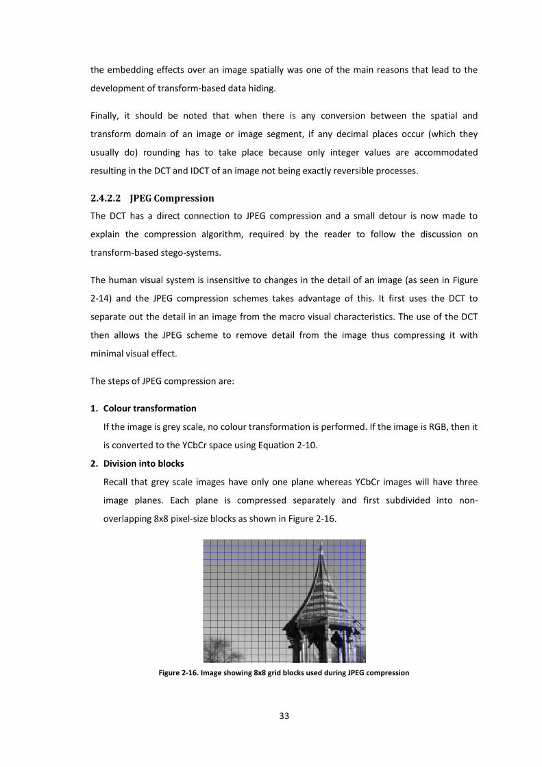
33
the embedding effects over an image spatially was one of the main reasons that lead to the
development of transform-based data hiding.
Finally, it should be noted that when there is any conversion between the spatial and
transform domain of an image or image segment, if any decimal places occur (which they
usually do) rounding has to take place because only integer values are accommodated
resulting in the DCT and IDCT of an image not being exactly reversible processes.
2.4.2.2 JPEG Compression
The DCT has a direct connection to JPEG compression and a small detour is now made to
explain the compression algorithm, required by the reader to follow the discussion on
transform-based stego-systems.
The human visual system is insensitive to changes in the detail of an image (as seen in Figure
2-14) and the JPEG compression schemes takes advantage of this. It first uses the DCT to
separate out the detail in an image from the macro visual characteristics. The use of the DCT
then allows the JPEG scheme to remove detail from the image thus compressing it with
minimal visual effect.
The steps of JPEG compression are:
1. Colour transformation
If the image is grey scale, no colour transformation is performed. If the image is RGB, then it
is converted to the YCbCr space using Equation 2-10.
2. Division into blocks
Recall that grey scale images have only one plane whereas YCbCr images will have three
image planes. Each plane is compressed separately and first subdivided into non-
overlapping 8x8 pixel-size blocks as shown in Figure 2-16.
Figure 2-16. Image showing 8x8 grid blocks used during JPEG compression
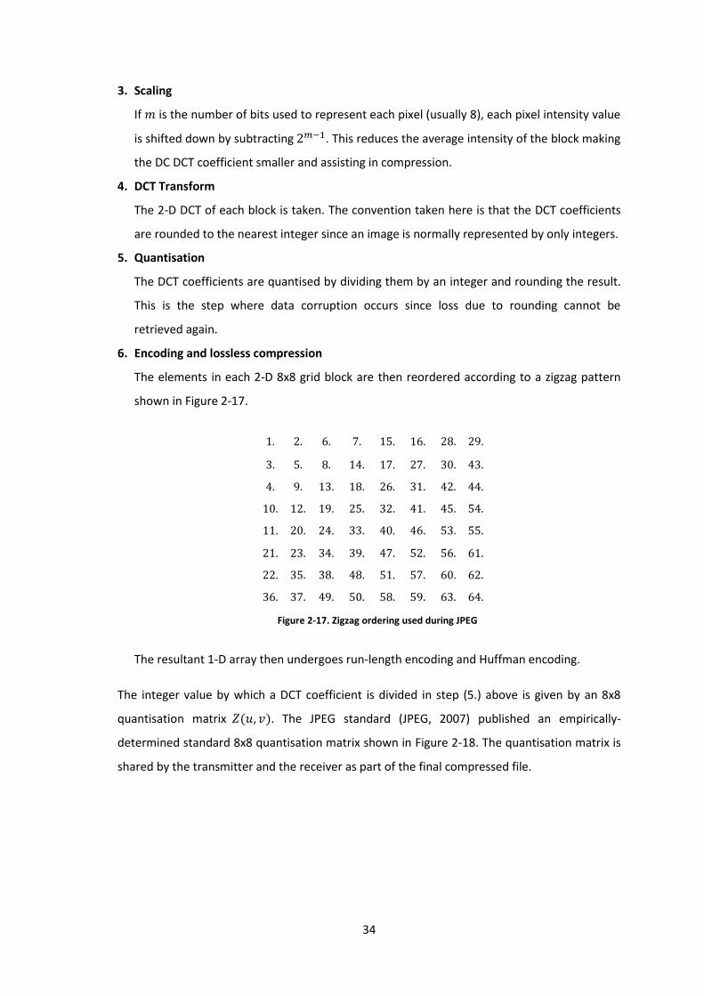
34
3. Scaling
If is the number of bits used to represent each pixel (usually 8), each pixel intensity value
is shifted down by subtracting . This reduces the average intensity of the block making
the DC DCT coefficient smaller and assisting in compression.
4. DCT Transform
The 2-D DCT of each block is taken. The convention taken here is that the DCT coefficients
are rounded to the nearest integer since an image is normally represented by only integers.
5. Quantisation
The DCT coefficients are quantised by dividing them by an integer and rounding the result.
This is the step where data corruption occurs since loss due to rounding cannot be
retrieved again.
6. Encoding and lossless compression
The elements in each 2-D 8x8 grid block are then reordered according to a zigzag pattern
shown in Figure 2-17.
1. 2. 6. 7. 15. 16. 28. 29.
3. 5. 8. 14. 17. 27. 30. 43.
4. 9. 13. 18. 26. 31. 42. 44.
10. 12. 19. 25. 32. 41. 45. 54.
11. 20. 24. 33. 40. 46. 53. 55.
21. 23. 34. 39. 47. 52. 56. 61.
22. 35. 38. 48. 51. 57. 60. 62.
36. 37. 49. 50. 58. 59. 63. 64.
Figure 2-17. Zigzag ordering used during JPEG
The resultant 1-D array then undergoes run-length encoding and Huffman encoding.
The integer value by which a DCT coefficient is divided in step (5.) above is given by an 8x8
quantisation matrix . The JPEG standard (JPEG, 2007) published an empirically-
determined standard 8x8 quantisation matrix shown in Figure 2-18. The quantisation matrix is
shared by the transmitter and the receiver as part of the final compressed file.
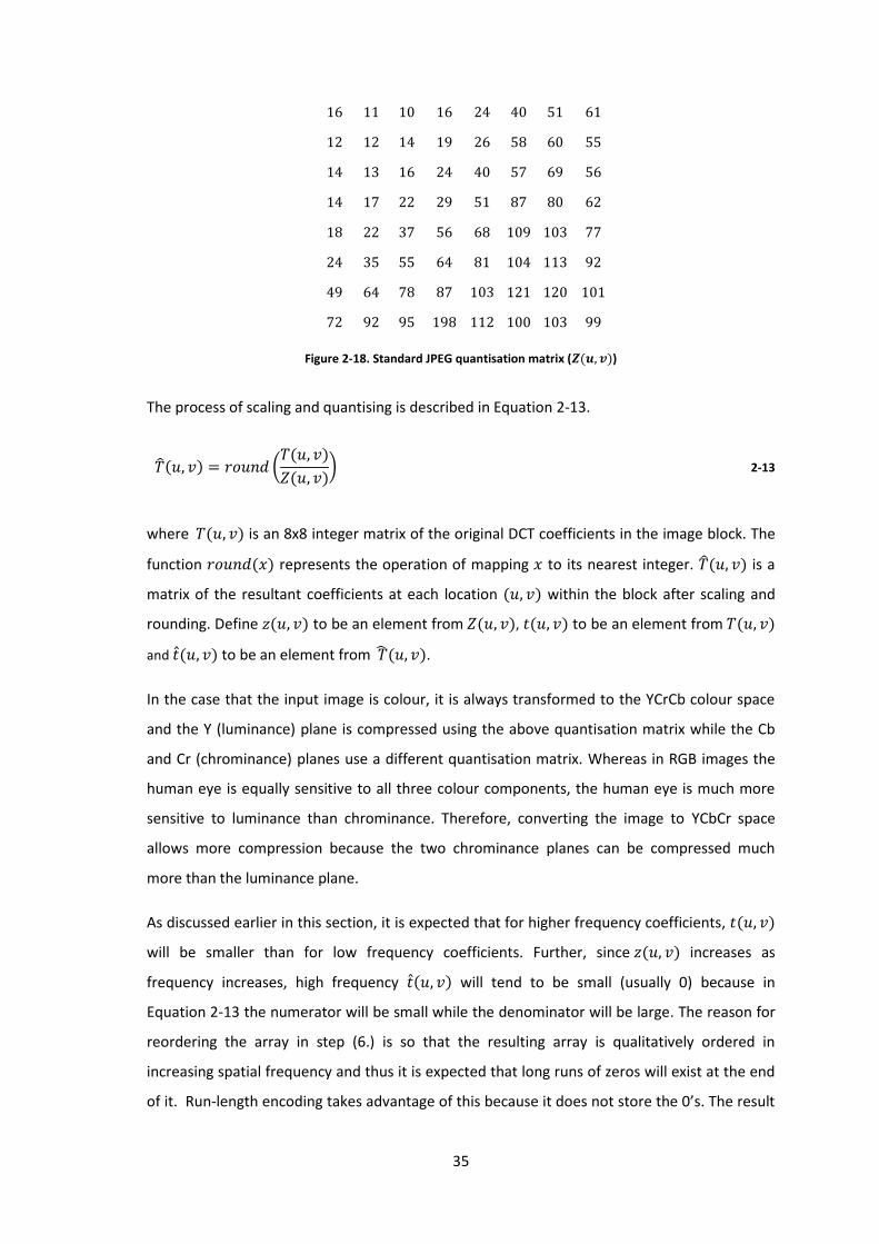
35
16 11 10 16 24 40 51 61
12 12 14 19 26 58 60 55
14 13 16 24 40 57 69 56
14 17 22 29 51 87 80 62
18 22 37 56 68 109 103 77
24 35 55 64 81 104 113 92
49 64 78 87 103 121 120 101
72 92 95 198 112 100 103 99
Figure 2-18. Standard JPEG quantisation matrix ( )
The process of scaling and quantising is described in Equation 2-13.
(
* 2-13
where is an 8x8 integer matrix of the original DCT coefficients in the image block. The
function represents the operation of mapping to its nearest integer. is a
matrix of the resultant coefficients at each location within the block after scaling and
rounding. Define to be an element from , to be an element from
and to be an element from .
In the case that the input image is colour, it is always transformed to the YCrCb colour space
and the Y (luminance) plane is compressed using the above quantisation matrix while the Cb
and Cr (chrominance) planes use a different quantisation matrix. Whereas in RGB images the
human eye is equally sensitive to all three colour components, the human eye is much more
sensitive to luminance than chrominance. Therefore, converting the image to YCbCr space
allows more compression because the two chrominance planes can be compressed much
more than the luminance plane.
As discussed earlier in this section, it is expected that for higher frequency coefficients,
will be smaller than for low frequency coefficients. Further, since increases as
frequency increases, high frequency will tend to be small (usually 0) because in
Equation 2-13 the numerator will be small while the denominator will be large. The reason for
reordering the array in step (6.) is so that the resulting array is qualitatively ordered in
increasing spatial frequency and thus it is expected that long runs of zeros will exist at the end
of it. Run-length encoding takes advantage of this because it does not store the 0’s. The result
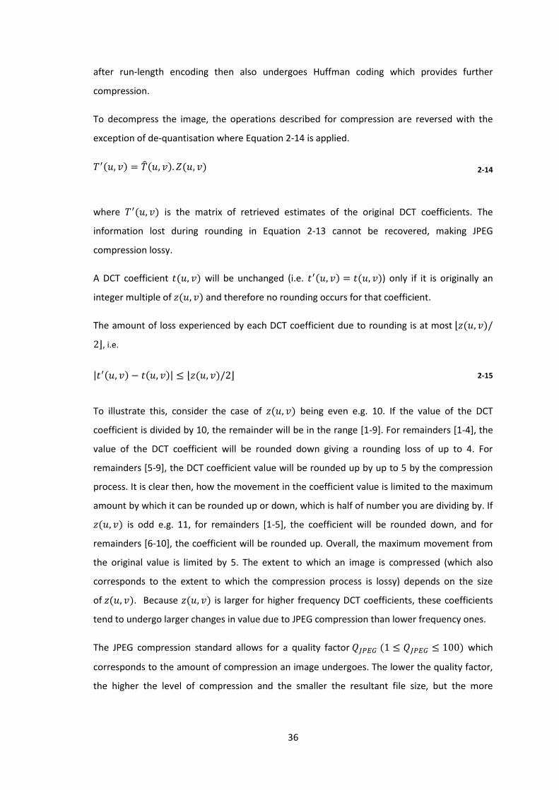
36
after run-length encoding then also undergoes Huffman coding which provides further
compression.
To decompress the image, the operations described for compression are reversed with the
exception of de-quantisation where Equation 2-14 is applied.
2-14
where is the matrix of retrieved estimates of the original DCT coefficients. The
information lost during rounding in Equation 2-13 cannot be recovered, making JPEG
compression lossy.
A DCT coefficient will be unchanged (i.e. ) only if it is originally an
integer multiple of and therefore no rounding occurs for that coefficient.
The amount of loss experienced by each DCT coefficient due to rounding is at most ⌊
⌋, i.e.
⌊ ⌋ 2-15
To illustrate this, consider the case of being even e.g. 10. If the value of the DCT
coefficient is divided by 10, the remainder will be in the range [1-9]. For remainders [1-4], the
value of the DCT coefficient will be rounded down giving a rounding loss of up to 4. For
remainders [5-9], the DCT coefficient value will be rounded up by up to 5 by the compression
process. It is clear then, how the movement in the coefficient value is limited to the maximum
amount by which it can be rounded up or down, which is half of number you are dividing by. If
is odd e.g. 11, for remainders [1-5], the coefficient will be rounded down, and for
remainders [6-10], the coefficient will be rounded up. Overall, the maximum movement from
the original value is limited by 5. The extent to which an image is compressed (which also
corresponds to the extent to which the compression process is lossy) depends on the size
of . Because is larger for higher frequency DCT coefficients, these coefficients
tend to undergo larger changes in value due to JPEG compression than lower frequency ones.
The JPEG compression standard allows for a quality factor which
corresponds to the amount of compression an image undergoes. The lower the quality factor,
the higher the level of compression and the smaller the resultant file size, but the more
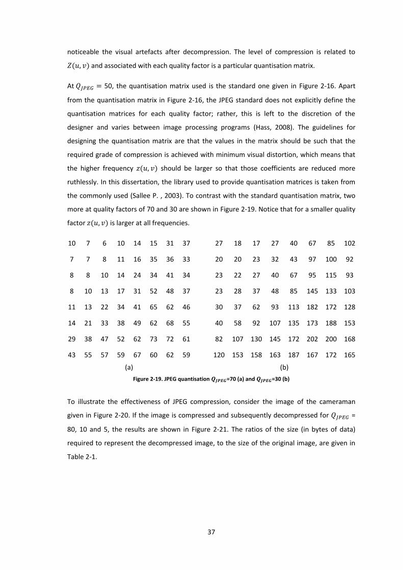
37
noticeable the visual artefacts after decompression. The level of compression is related to
and associated with each quality factor is a particular quantisation matrix.
At 50, the quantisation matrix used is the standard one given in Figure 2-16. Apart
from the quantisation matrix in Figure 2-16, the JPEG standard does not explicitly define the
quantisation matrices for each quality factor; rather, this is left to the discretion of the
designer and varies between image processing programs (Hass, 2008). The guidelines for
designing the quantisation matrix are that the values in the matrix should be such that the
required grade of compression is achieved with minimum visual distortion, which means that
the higher frequency should be larger so that those coefficients are reduced more
ruthlessly. In this dissertation, the library used to provide quantisation matrices is taken from
the commonly used (Sallee P. , 2003). To contrast with the standard quantisation matrix, two
more at quality factors of 70 and 30 are shown in Figure 2-19. Notice that for a smaller quality
factor is larger at all frequencies.
10 7 6 10 14 15 31 37 27 18 17 27 40 67 85 102
7 7 8 11 16 35 36 33 20 20 23 32 43 97 100 92
8 8 10 14 24 34 41 34 23 22 27 40 67 95 115 93
8 10 13 17 31 52 48 37 23 28 37 48 85 145 133 103
11 13 22 34 41 65 62 46 30 37 62 93 113 182 172 128
14 21 33 38 49 62 68 55 40 58 92 107 135 173 188 153
29 38 47 52 62 73 72 61 82 107 130 145 172 202 200 168
43 55 57 59 67 60 62 59 120 153 158 163 187 167 172 165
(a) (b)
Figure 2-19. JPEG quantisation =70 (a) and =30 (b)
To illustrate the effectiveness of JPEG compression, consider the image of the cameraman
given in Figure 2-20. If the image is compressed and subsequently decompressed for =
80, 10 and 5, the results are shown in Figure 2-21. The ratios of the size (in bytes of data)
required to represent the decompressed image, to the size of the original image, are given in
Table 2-1.
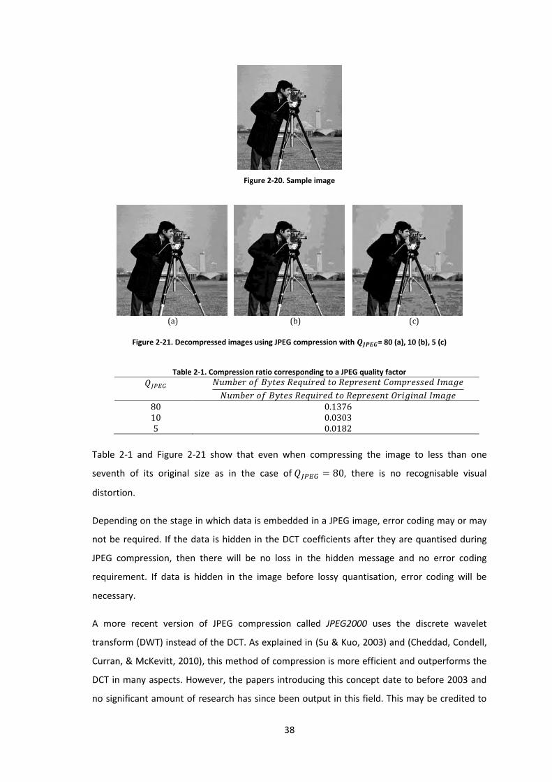
38
Figure 2-20. Sample image
Figure 2-21. Decompressed images using JPEG compression with = 80 (a), 10 (b), 5 (c)
Table 2-1. Compression ratio corresponding to a JPEG quality factor
80 0.1376 10 0.0303 5 0.0182
Table 2-1 and Figure 2-21 show that even when compressing the image to less than one
seventh of its original size as in the case of , there is no recognisable visual
distortion.
Depending on the stage in which data is embedded in a JPEG image, error coding may or may
not be required. If the data is hidden in the DCT coefficients after they are quantised during
JPEG compression, then there will be no loss in the hidden message and no error coding
requirement. If data is hidden in the image before lossy quantisation, error coding will be
necessary.
A more recent version of JPEG compression called JPEG2000 uses the discrete wavelet
transform (DWT) instead of the DCT. As explained in (Su & Kuo, 2003) and (Cheddad, Condell,
Curran, & McKevitt, 2010), this method of compression is more efficient and outperforms the
DCT in many aspects. However, the papers introducing this concept date to before 2003 and
no significant amount of research has since been output in this field. This may be credited to
(a) (b) (c)
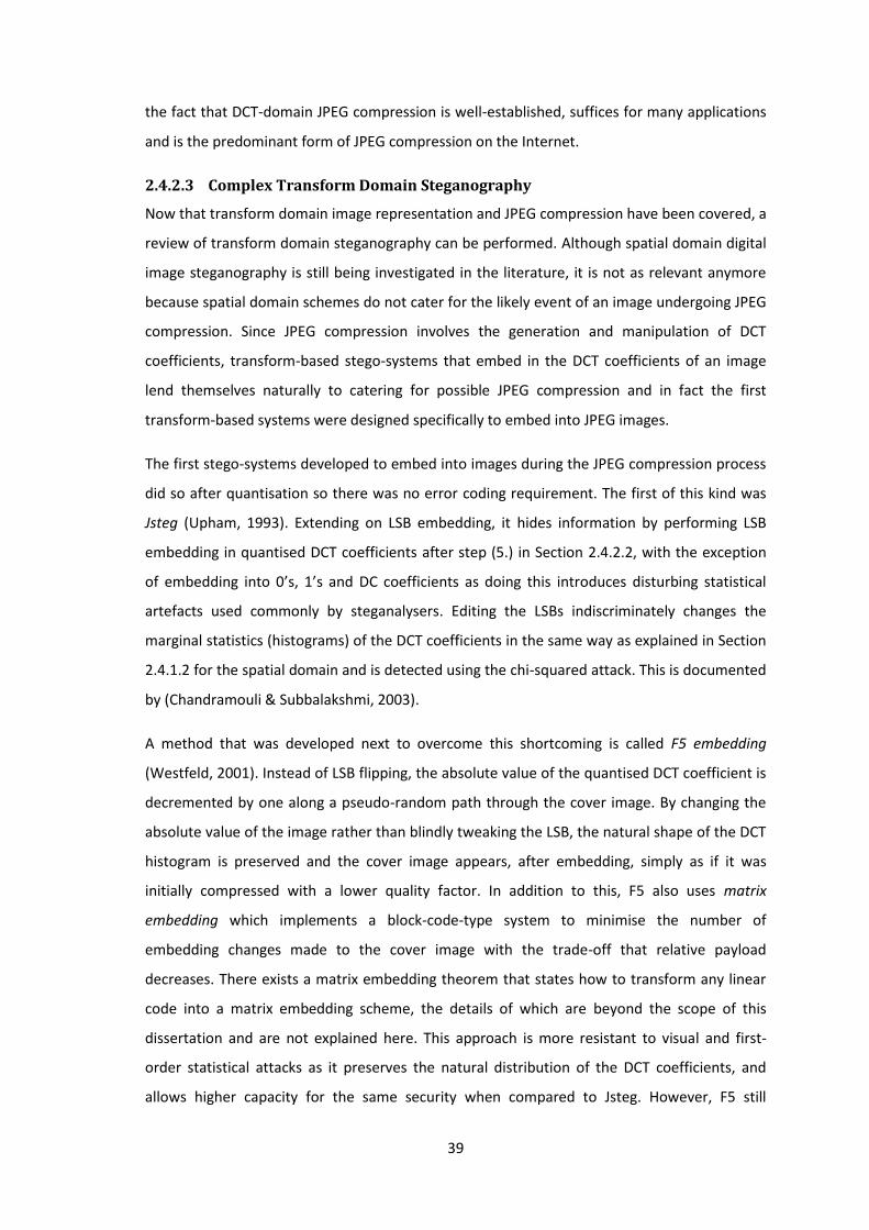
39
the fact that DCT-domain JPEG compression is well-established, suffices for many applications
and is the predominant form of JPEG compression on the Internet.
2.4.2.3 Complex Transform Domain Steganography
Now that transform domain image representation and JPEG compression have been covered, a
review of transform domain steganography can be performed. Although spatial domain digital
image steganography is still being investigated in the literature, it is not as relevant anymore
because spatial domain schemes do not cater for the likely event of an image undergoing JPEG
compression. Since JPEG compression involves the generation and manipulation of DCT
coefficients, transform-based stego-systems that embed in the DCT coefficients of an image
lend themselves naturally to catering for possible JPEG compression and in fact the first
transform-based systems were designed specifically to embed into JPEG images.
The first stego-systems developed to embed into images during the JPEG compression process
did so after quantisation so there was no error coding requirement. The first of this kind was
Jsteg (Upham, 1993). Extending on LSB embedding, it hides information by performing LSB
embedding in quantised DCT coefficients after step (5.) in Section 2.4.2.2, with the exception
of embedding into 0’s, 1’s and DC coefficients as doing this introduces disturbing statistical
artefacts used commonly by steganalysers. Editing the LSBs indiscriminately changes the
marginal statistics (histograms) of the DCT coefficients in the same way as explained in Section
2.4.1.2 for the spatial domain and is detected using the chi-squared attack. This is documented
by (Chandramouli & Subbalakshmi, 2003).
A method that was developed next to overcome this shortcoming is called F5 embedding
(Westfeld, 2001). Instead of LSB flipping, the absolute value of the quantised DCT coefficient is
decremented by one along a pseudo-random path through the cover image. By changing the
absolute value of the image rather than blindly tweaking the LSB, the natural shape of the DCT
histogram is preserved and the cover image appears, after embedding, simply as if it was
initially compressed with a lower quality factor. In addition to this, F5 also uses matrix
embedding which implements a block-code-type system to minimise the number of
embedding changes made to the cover image with the trade-off that relative payload
decreases. There exists a matrix embedding theorem that states how to transform any linear
code into a matrix embedding scheme, the details of which are beyond the scope of this
dissertation and are not explained here. This approach is more resistant to visual and first-
order statistical attacks as it preserves the natural distribution of the DCT coefficients, and
allows higher capacity for the same security when compared to Jsteg. However, F5 still
40
changes the histogram in a detectable way as shown by (Fridrich, Goljan, & Hogea, 2003) and
(Dabeer, Sullivan, Madhow, Chandrasekaran, & Manjunath, 2004) and can be detected by
comparing the stego-image histogram to an estimate of the original histogram. The original
histogram is estimated using a self-calibrating method: the JPEG stego-image is decompressed
and cropped by a few pixel rows or columns in order to desynchronise it from the original JPEG
grid. If this cropped image is then recompressed, the statistical properties of the resultant
image are similar to those of the original cover image and can be compared to the suspicious
stego-image (Fridrich, Goljan, & Hogea, 2003).
Another system, OutGuess (Provos, 2000), was the first system whose goal was specifically to
match the DCT histogram of the cover image. It embeds messages into the cover image by
slightly changing the quantized DCT coefficients using two runs. Firstly, the message bits are
embedded into a pseudo-random set of DCT coefficients. In the second run, corrections are
made to other DCT coefficients in order to match the stego-image histogram with that of the
cover image. So if a particular coefficient is changed from histogram bin A to B during
embedding, the correction for this would be to move another coefficient from bin B to A.
OutGuess uses about half of the coefficients for embedding and the other half for correcting
statistical deviations. This technique is effective in maintaining the DCT coefficient histogram
but reduces the effective capacity by half and can be broken by second order statistical
analysis (Hetzl & Mutzel, 2005).
Steghide, introduced in (Hetzl & Mutzel, 2005), also preserves global first-order statistics of
DCT coefficients using a different mechanism to OutGuess. Coefficients are swapped rather
than having their LSB modified.
Another proposed system is called Model-Based Steganography (Sallee P. , 2004) which
assumes a more abstract mathematical approach that edits coefficient values with the primary
goal of maintaining the original statistical composition of the coefficients. (Fridrich J. , Goljan,
Lisoňek, & Soukal, 2004) present an approach that uses perturbed quantisation where the way
in which quantisation of the DCT coefficients occurs is slightly perturbed to embed secret
message bits. (Solanki K. , Sullivan, Madhow, Manjunath, & Chandrasekaran, 2005) and
(Solanki K. , Sullivan, Madhow, Manjunath, & Chandrasekaran, 2006) introduce mathematical
schemes that match the DCT histogram of the stego-image to that of the cover image exactly,
providing provable security only if the steganalyst uses properties of the DCT histogram for
detection.
41
Adaptive embedding in the frequency domain developed from the discussed schemes is not a
well-developed topic in contrast to the spatial domain. Typical examples include (Kumar, Raja,
Chhotaray, & Pattnaik, 2010) where varying amounts of bits are embedded in coefficients
depending on their size, and (Velasco, Nakano, Perez, Martinez, & Yamaguchi, 2009) which
uses the energy of the DCT coefficients as a metric.
Stego-systems may also use the compression process itself to embed information. For
example, (Guo & Le, 2010) uses various quantisation tables for different regions of the JPEG-
compressed image to provide information that achieves satisfactory performance while
simplifying the embedding process.
2.4.2.4 Cell-Based Systems
So far, the stego-systems have focused on hiding data with the purpose of camouflaging some
statistical artefacts of embedding. In general, blind statistical steganalysis schemes have been
very successful in detecting these types of stego-systems.
As explained in (Solanki, Sarkar, & Manjunath, 2007), the elements that contribute to the
success of blind steganalysers are:
Self-calibration mechanism
With this mechanism, the blind steganalysers make an estimate of the original statistics of
the cover image. In the case of JPEG images, the self-calibration technique of cropping and
recompressing the image mentioned earlier is used.
Features capturing cover memory
Some steganographic systems hide data symbols rather than individual bits and the blind
steganalyser can use any known statistical properties of the symbol bits to detect trends in
statistical changes. Cover memory has been shown to be an important feature (Sullivan,
Madhow, Chandrasekaran, & Manjunath, 2006) and has been incorporated into the feature
vector for training (e.g. (Fu, Shi, Zou, & Xuan, 2006), (Shi, Chen, & Chen, 2006)).
Powerful machine learning
The existence of powerful machine learning techniques combined with training over several
thousand images often ensures even slight statistical variations become learned by the
analyser.
The most prominent of the above elements is the ability of the blind analyser to use certain
assumptions about the image to get a model of the innocent cover image despite not having
access to it and even though no universal statistical model for images exists.
42
To address this, (Solanki, Sarkar, & Manjunath, 2007) suggest that instead of the approach
used by stego-systems so far to try to maintain statistical features of the cover image, a
steganographer can take the approach of attempting to distort the blind steganalyst’s estimate
of the innocent cover image statistics in two ways:
1. Hiding with high embedding strength
Instead of minimising embedding artefacts, if embedding is performed so that the cover
image is so distorted that cover image statistics can no longer be derived then detection
will be more difficult for the blind steganalyser. (Kharrazi, Sencar, & Memon, 2006) show
that this is possible.
2. Randomised hiding
If the embedding approach is randomised then the steganalyst cannot make any consistent
assumptions regarding how data has been hidden even if the stego-algorithm is known as
per Kerckhoffs’ principle.
The danger of the first approach above is that the likelihood of embedding artefacts being
visually perceptible is high and it’s possible the image can be detected by a steganalyst with a
universal image model even if it is very rough. The second approach is more appealing and
(Solanki, Sarkar, & Manjunath, 2007) explore the first simplest implementation of this by
randomising the locations where data is hidden in an image. This implementation is called Yet
Another Steganographic System (YASS) and is the earliest of the cell-based systems so called
because embedding occurs in certain randomly-selected blocks/cells in an image.
In addition to the randomised approach to embedding, cell-based systems embed into an
image before the lossy stage of JPEG compression which further disguises embedding artefacts
since the analyser would examine the stego-image after compression. This also means error
coding is required to cater for lossy JPEG compression. (Huang, Huang, & Qing Shi, 2010) and
(Fridrich & Kodovsky, 2008) say YASS is arguably one of the most promising transform domain-
based systems to date and the security of this method against advanced blind steganalysis
systems has gained attention in the research community in the past two years (e.g. (Li, Huang,
& Shi, 2009), (Huang, Huang, & Shi, 2010)). Only one other paper (Sajedi & Jamzad, 2010) was
found that uses the philosophy of randomising where data is hidden but YASS has gained much
more interest and is the focus here.
The input image to YASS is grey scale or, if not, the Y plane is extracted and used to carry
secret data since it is the least-aggressively compressed plane during JPEG compression
resulting in lower errors.
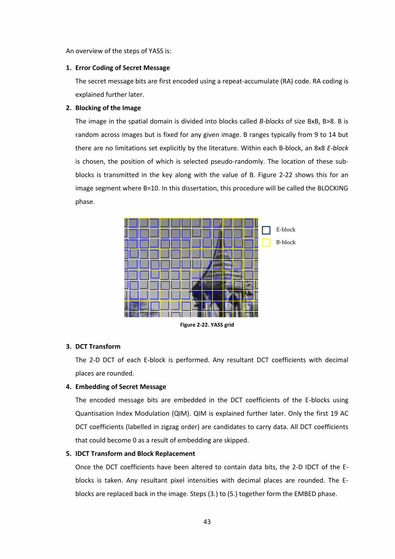
43
An overview of the steps of YASS is:
1. Error Coding of Secret Message
The secret message bits are first encoded using a repeat-accumulate (RA) code. RA coding is
explained further later.
2. Blocking of the Image
The image in the spatial domain is divided into blocks called B-blocks of size BxB, B>8. B is
random across images but is fixed for any given image. B ranges typically from 9 to 14 but
there are no limitations set explicitly by the literature. Within each B-block, an 8x8 E-block
is chosen, the position of which is selected pseudo-randomly. The location of these sub-
blocks is transmitted in the key along with the value of B. Figure 2-22 shows this for an
image segment where B=10. In this dissertation, this procedure will be called the BLOCKING
phase.
Figure 2-22. YASS grid
3. DCT Transform
The 2-D DCT of each E-block is performed. Any resultant DCT coefficients with decimal
places are rounded.
4. Embedding of Secret Message
The encoded message bits are embedded in the DCT coefficients of the E-blocks using
Quantisation Index Modulation (QIM). QIM is explained further later. Only the first 19 AC
DCT coefficients (labelled in zigzag order) are candidates to carry data. All DCT coefficients
that could become 0 as a result of embedding are skipped.
5. IDCT Transform and Block Replacement
Once the DCT coefficients have been altered to contain data bits, the 2-D IDCT of the E-
blocks is taken. Any resultant pixel intensities with decimal places are rounded. The E-
blocks are replaced back in the image. Steps (3.) to (5.) together form the EMBED phase.
E-block
B-block
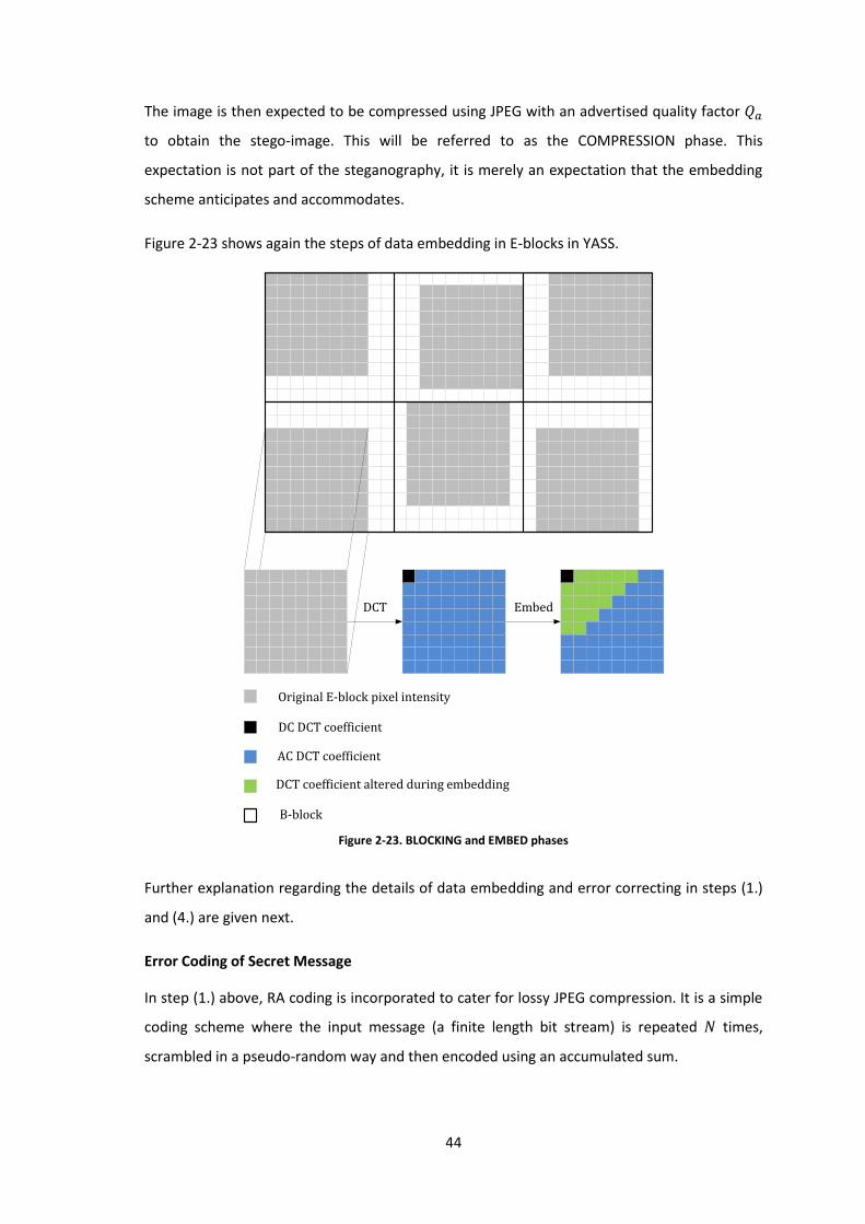
44
The image is then expected to be compressed using JPEG with an advertised quality factor
to obtain the stego-image. This will be referred to as the COMPRESSION phase. This
expectation is not part of the steganography, it is merely an expectation that the embedding
scheme anticipates and accommodates.
Figure 2-23 shows again the steps of data embedding in E-blocks in YASS.
Figure 2-23. BLOCKING and EMBED phases
Further explanation regarding the details of data embedding and error correcting in steps (1.)
and (4.) are given next.
Error Coding of Secret Message
In step (1.) above, RA coding is incorporated to cater for lossy JPEG compression. It is a simple
coding scheme where the input message (a finite length bit stream) is repeated times,
scrambled in a pseudo-random way and then encoded using an accumulated sum.
Original E-block pixel intensity
DC DCT coefficient
AC DCT coefficient
DCT coefficient altered during embedding
B-block
DCT Embed
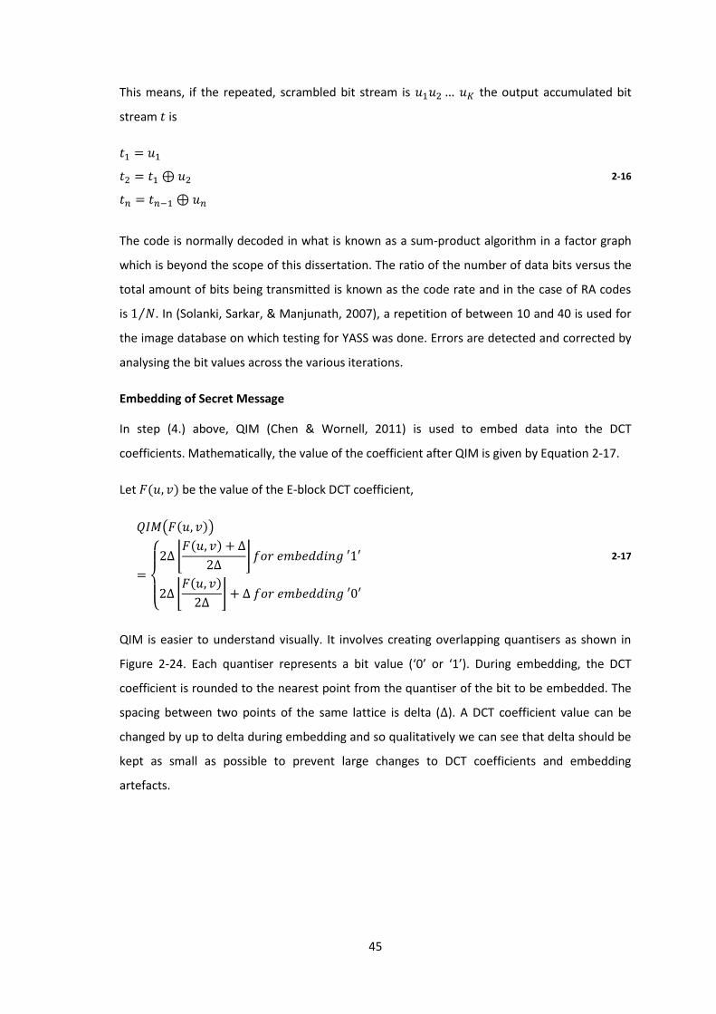
45
This means, if the repeated, scrambled bit stream is the output accumulated bit
stream is
2-16
The code is normally decoded in what is known as a sum-product algorithm in a factor graph
which is beyond the scope of this dissertation. The ratio of the number of data bits versus the
total amount of bits being transmitted is known as the code rate and in the case of RA codes
is ⁄ . In (Solanki, Sarkar, & Manjunath, 2007), a repetition of between 10 and 40 is used for
the image database on which testing for YASS was done. Errors are detected and corrected by
analysing the bit values across the various iterations.
Embedding of Secret Message
In step (4.) above, QIM (Chen & Wornell, 2011) is used to embed data into the DCT
coefficients. Mathematically, the value of the coefficient after QIM is given by Equation 2-17.
Let be the value of the E-block DCT coefficient,
( )
{
⌊
⌋
⌊
⌋
2-17
QIM is easier to understand visually. It involves creating overlapping quantisers as shown in
Figure 2-24. Each quantiser represents a bit value (‘0’ or ‘1’). During embedding, the DCT
coefficient is rounded to the nearest point from the quantiser of the bit to be embedded. The
spacing between two points of the same lattice is delta ( ). A DCT coefficient value can be
changed by up to delta during embedding and so qualitatively we can see that delta should be
kept as small as possible to prevent large changes to DCT coefficients and embedding
artefacts.
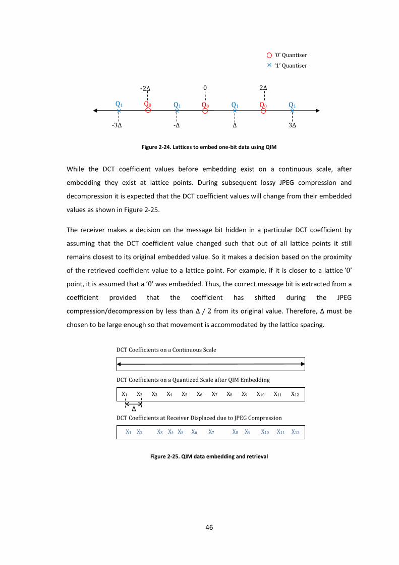
46
Figure 2-24. Lattices to embed one-bit data using QIM
While the DCT coefficient values before embedding exist on a continuous scale, after
embedding they exist at lattice points. During subsequent lossy JPEG compression and
decompression it is expected that the DCT coefficient values will change from their embedded
values as shown in Figure 2-25.
The receiver makes a decision on the message bit hidden in a particular DCT coefficient by
assuming that the DCT coefficient value changed such that out of all lattice points it still
remains closest to its original embedded value. So it makes a decision based on the proximity
of the retrieved coefficient value to a lattice point. For example, if it is closer to a lattice
point, it is assumed that a was embedded. Thus, the correct message bit is extracted from a
coefficient provided that the coefficient has shifted during the JPEG
compression/decompression by less than ⁄ from its original value. Therefore, Δ must be
chosen to be large enough so that movement is accommodated by the lattice spacing.
Figure 2-25. QIM data embedding and retrieval
Q1 Q1 Q0
Q0 Q0 Q1 Q1
- -
0 -
‘0’ Quantiser
‘1’ Quantiser
DCT Coefficients on a Quantized Scale after QIM Embedding
X1 X2 X3 X4 X5 X6 X7 X8 X9 X10 X11 X12
∆
DCT Coefficients on a Continuous Scale
X1 X2 X3 X4 X5 X6 X7 X8 X9 X10 X11 X12
DCT Coefficients at Receiver Displaced due to JPEG Compression
47
The change in data carrying E-block DCT coefficient value between QIM embedding and QIM
de-embedding is caused by two things:
1. Rounding after each conversion between the transform and spatial domains during the
EMBED phase. This is because the image representation does not accommodate decimal
places.
2. The effects of JPEG compression during the COMPRESSION phase, namely the harsher
treatment of higher frequency coefficients.
Out of the two causes of change in value of the data carrying DCT coefficients, rounding can
cause absolute value change of 1, while the effects of JPEG compression are much more
profound. The exact extent to which JPEG compression causes the data carrying DCT
coefficient value to change is required to determine an appropriate QIM system and is
investigated in Chapter 3.
Roughly speaking, since higher frequency coefficients experience more error (change in value)
due to JPEG compression, it would make sense to use a larger delta for these coefficients than
for low frequency ones. The values of delta used by YASS have purposefully not been explained
here because some further knowledge is required before this is understood by the reader and
therefore will be referred to in the next chapter where for now only the concept is important.
It was stated that during the EMBED phase, not all of the 19 candidate AC DCT coefficients in
an E-block are necessarily used to carry data. Specifically, candidate coefficients in the range
are at risk of being quantised to 0 during embedding and so are rejected. This is to
prevent the embedding scheme from changing the number and distribution of DCT coefficients
of value 0 which has been used previously as a statistical artefact for detection by
steganalysers. In this dissertation, the requirement that a candidate E-block DCT coefficient be
outside the range in order to be selected to carry data will be referred to as selection
criteria.
Embedding into the DC DCT coefficient is also forbidden to prevent statistical boundaries in
variation of average colour that can be easily detected by analysers. In Figure 2-26, the DC
coefficient in a block was decreased by 10, and clear visual (and thus also statistical)
boundaries exist, providing an obvious give-away embedding artefact that should be avoided.
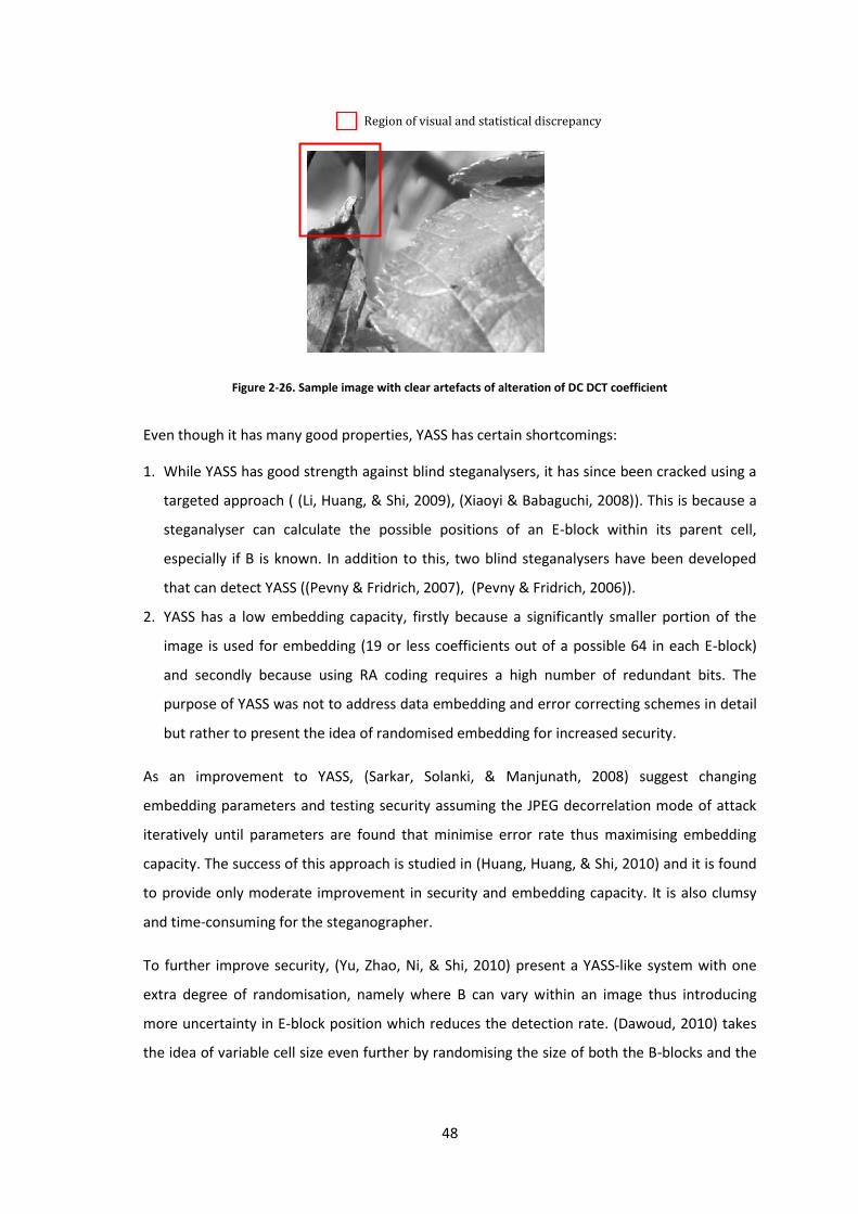
48
Figure 2-26. Sample image with clear artefacts of alteration of DC DCT coefficient
Even though it has many good properties, YASS has certain shortcomings:
1. While YASS has good strength against blind steganalysers, it has since been cracked using a
targeted approach ( (Li, Huang, & Shi, 2009), (Xiaoyi & Babaguchi, 2008)). This is because a
steganalyser can calculate the possible positions of an E-block within its parent cell,
especially if B is known. In addition to this, two blind steganalysers have been developed
that can detect YASS ((Pevny & Fridrich, 2007), (Pevny & Fridrich, 2006)).
2. YASS has a low embedding capacity, firstly because a significantly smaller portion of the
image is used for embedding (19 or less coefficients out of a possible 64 in each E-block)
and secondly because using RA coding requires a high number of redundant bits. The
purpose of YASS was not to address data embedding and error correcting schemes in detail
but rather to present the idea of randomised embedding for increased security.
As an improvement to YASS, (Sarkar, Solanki, & Manjunath, 2008) suggest changing
embedding parameters and testing security assuming the JPEG decorrelation mode of attack
iteratively until parameters are found that minimise error rate thus maximising embedding
capacity. The success of this approach is studied in (Huang, Huang, & Shi, 2010) and it is found
to provide only moderate improvement in security and embedding capacity. It is also clumsy
and time-consuming for the steganographer.
To further improve security, (Yu, Zhao, Ni, & Shi, 2010) present a YASS-like system with one
extra degree of randomisation, namely where B can vary within an image thus introducing
more uncertainty in E-block position which reduces the detection rate. (Dawoud, 2010) takes
the idea of variable cell size even further by randomising the size of both the B-blocks and the
Region of visual and statistical discrepancy
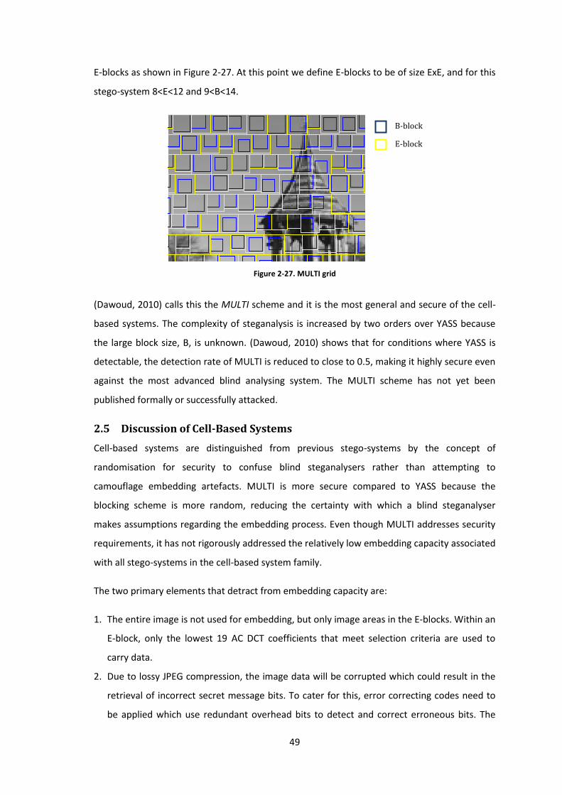
49
E-blocks as shown in Figure 2-27. At this point we define E-blocks to be of size ExE, and for this
stego-system 8<E<12 and 9<B<14.
Figure 2-27. MULTI grid
(Dawoud, 2010) calls this the MULTI scheme and it is the most general and secure of the cell-
based systems. The complexity of steganalysis is increased by two orders over YASS because
the large block size, B, is unknown. (Dawoud, 2010) shows that for conditions where YASS is
detectable, the detection rate of MULTI is reduced to close to 0.5, making it highly secure even
against the most advanced blind analysing system. The MULTI scheme has not yet been
published formally or successfully attacked.
2.5 Discussion of Cell-Based Systems
Cell-based systems are distinguished from previous stego-systems by the concept of
randomisation for security to confuse blind steganalysers rather than attempting to
camouflage embedding artefacts. MULTI is more secure compared to YASS because the
blocking scheme is more random, reducing the certainty with which a blind steganalyser
makes assumptions regarding the embedding process. Even though MULTI addresses security
requirements, it has not rigorously addressed the relatively low embedding capacity associated
with all stego-systems in the cell-based system family.
The two primary elements that detract from embedding capacity are:
1. The entire image is not used for embedding, but only image areas in the E-blocks. Within an
E-block, only the lowest 19 AC DCT coefficients that meet selection criteria are used to
carry data.
2. Due to lossy JPEG compression, the image data will be corrupted which could result in the
retrieval of incorrect secret message bits. To cater for this, error correcting codes need to
be applied which use redundant overhead bits to detect and correct erroneous bits. The
B-block
E-block
50
inclusion of these overhead bits further reduces the number of information bits that can be
accommodated.
The two data handling issues presented above have not been rigorously addressed in the
literature so far. It should be noted that the focus of the literature around cell-based systems
has not been on embedding capacity in particular and so no claims have been made that the
used data handling systems are optimal.
In particular, the values of delta using during QIM for YASS and MULTI have been estimated
simplistically. Given the effect of JPEG compression, it is expected that as coefficients increase
in frequency a larger delta for QIM would be required since they are likely to experience more
error. YASS does use larger delta for higher frequency coefficients (the details will be referred
to in Chapter 3) but the suitability of the delta values was not analysed.
Regarding the number of DCT coefficients considered for embedding, there is no evidence that
only the first 19 low frequency coefficients are appropriate, and it is viable to suspect more
vulnerable higher frequency coefficients may provide increased embedding capacity if the
correct error coding is used. (Sarkar, Nataraj, Manjunath, & Madhow, 2008) suggest analysing
the potential of different E-block coefficients to carry data but do not take the idea further.
There is no evidence that RA coding is the most efficient in terms of embedding capacity and
to the contrary the code rates appear low compared to other possible coding schemes. The
choice of code rates is also made based on characteristics of image segments or entire images
which considering the effect of JPEG compression appears to be inefficient. To illustrate this,
consider that within any image segment, different frequencies of DCT coefficients will be
treated differently by JPEG compression. More specifically, higher frequency DCT coefficients
will experience more change in value due to JPEG compression than lower frequency
coefficients according to the principles of JPEG that state the visual integrity of the image
should be preserved. Therefore, the likelihood and concentrations of errors in the DCT
coefficients will vary across a segment. At first sight it seems inefficient to design one coding
scheme to cater for the wide range of error in different parts of the image segment. These
issues regarding effective data embedding and error coding are discussed in detail in the next
chapter.
2.6 Summary
This chapter has described the assumed restrictions on stego-systems considered in this
research and presented a system model with related terminology. In particular, a private-key
51
stego-system by cover modification with a passive warden is assumed. The characteristics of a
successful stego-system, namely perceptibility, robustness and capacity are described.
Although initially visual perceptibility was a pertinent characteristic, the field has developed
such that the battle between steganography and steganalysis exists now on a more subtle,
statistical level. The term detectability is defined to mean susceptibility of a scheme to
statistical analysis whereas perceptibility is defined to be limited to the extent to which
embedding artefacts are visible.
The development of steganography and steganalysis can be traced from naïve and focused on
perceptibility to more complex and focused on detectability. In particular, naïve stego-systems
were based in the spatial domain and over time developed into more adaptive systems. With
the advent of effective image compression techniques, digital images are seldom transmitted
in the spatial domain anymore but in compressed versions where the image has been
transformed into the frequency (transform) domain. Within the field of transform-based
stego-systems, cell-based systems distinguish themselves from previous JPEG stego-systems by
embedding not with the purpose of maintaining cover image properties, but by randomising
the embedding process so that blind steganalysers aren’t able to estimate original cover image
properties. Cell-based systems are able to achieve high security by randomising embedding
locations and by hiding data before lossy JPEG compression, with the disadvantage that
embedding capacity is compromised. The lack of analytic reasoning in the selection of
coefficients for embedding, delta for QIM and error coding provides opportunity for research.
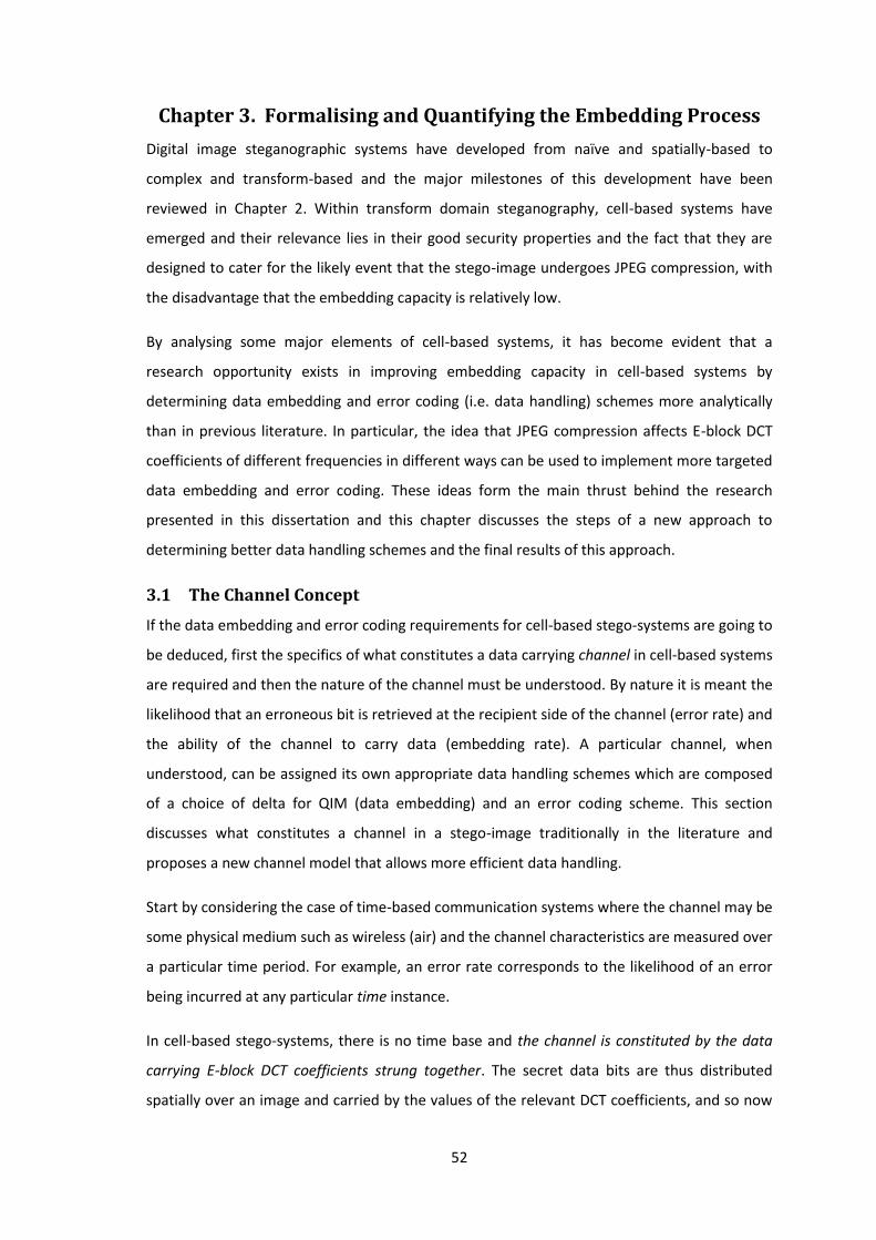
52
Chapter 3. Formalising and Quantifying the Embedding Process
Digital image steganographic systems have developed from naïve and spatially-based to
complex and transform-based and the major milestones of this development have been
reviewed in Chapter 2. Within transform domain steganography, cell-based systems have
emerged and their relevance lies in their good security properties and the fact that they are
designed to cater for the likely event that the stego-image undergoes JPEG compression, with
the disadvantage that the embedding capacity is relatively low.
By analysing some major elements of cell-based systems, it has become evident that a
research opportunity exists in improving embedding capacity in cell-based systems by
determining data embedding and error coding (i.e. data handling) schemes more analytically
than in previous literature. In particular, the idea that JPEG compression affects E-block DCT
coefficients of different frequencies in different ways can be used to implement more targeted
data embedding and error coding. These ideas form the main thrust behind the research
presented in this dissertation and this chapter discusses the steps of a new approach to
determining better data handling schemes and the final results of this approach.
3.1 The Channel Concept
If the data embedding and error coding requirements for cell-based stego-systems are going to
be deduced, first the specifics of what constitutes a data carrying channel in cell-based systems
are required and then the nature of the channel must be understood. By nature it is meant the
likelihood that an erroneous bit is retrieved at the recipient side of the channel (error rate) and
the ability of the channel to carry data (embedding rate). A particular channel, when
understood, can be assigned its own appropriate data handling schemes which are composed
of a choice of delta for QIM (data embedding) and an error coding scheme. This section
discusses what constitutes a channel in a stego-image traditionally in the literature and
proposes a new channel model that allows more efficient data handling.
Start by considering the case of time-based communication systems where the channel may be
some physical medium such as wireless (air) and the channel characteristics are measured over
a particular time period. For example, an error rate corresponds to the likelihood of an error
being incurred at any particular time instance.
In cell-based stego-systems, there is no time base and the channel is constituted by the data
carrying E-block DCT coefficients strung together. The secret data bits are thus distributed
spatially over an image and carried by the values of the relevant DCT coefficients, and so now
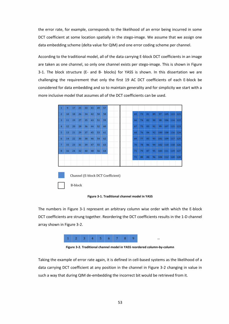
53
the error rate, for example, corresponds to the likelihood of an error being incurred in some
DCT coefficient at some location spatially in the stego-image. We assume that we assign one
data embedding scheme (delta value for QIM) and one error coding scheme per channel.
According to the traditional model, all of the data carrying E-block DCT coefficients in an image
are taken as one channel, so only one channel exists per stego-image. This is shown in Figure
3-1. The block structure (E- and B- blocks) for YASS is shown. In this dissertation we are
challenging the requirement that only the first 19 AC DCT coefficients of each E-block be
considered for data embedding and so to maintain generality and for simplicity we start with a
more inclusive model that assumes all of the DCT coefficients can be used.
1 9 17 25 33 41 49 57
2 18 26 34 42 50 58
3 11 19 27 35 43 51 59
4 12 20 28 36 44 52 60
5 13 21 29 37 45 53 61
6 14 22 30 38 46 54 62
7 15 23 31 39 47 55 63
8 16 24 32 40 48 56 64
65 73 81 89 97 105
66 74 82 90 98 106
67 75 83 91 99 107
68 76 84 92 100 108
69 77 85 93 101 109
70 78 86 94 102 110
71 79 87 95 103 111
72 80 88 96 104 112
113 121
114 122
115 123
116 124
117 125
118 126
119 127
120 128
10
Figure 3-1. Traditional channel model in YASS
The numbers in Figure 3-1 represent an arbitrary column wise order with which the E-block
DCT coefficients are strung together. Reordering the DCT coefficients results in the 1-D channel
array shown in Figure 3-2.
1 2 3 4 5 6 7 8 9 ...
Figure 3-2. Traditional channel model in YASS reordered column-by-column
Taking the example of error rate again, it is defined in cell-based systems as the likelihood of a
data carrying DCT coefficient at any position in the channel in Figure 3-2 changing in value in
such a way that during QIM de-embedding the incorrect bit would be retrieved from it.
Channel (E-block DCT Coefficient)
B-block
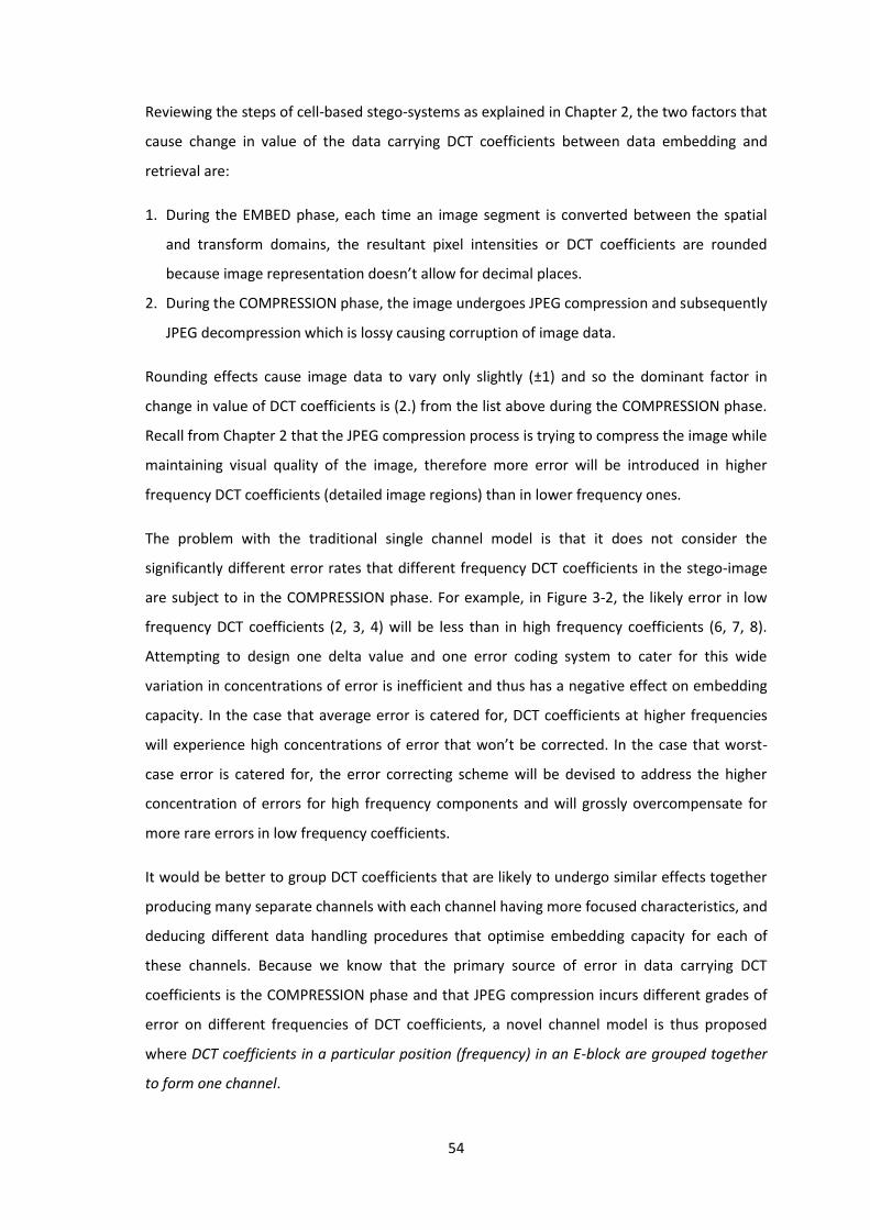
54
Reviewing the steps of cell-based stego-systems as explained in Chapter 2, the two factors that
cause change in value of the data carrying DCT coefficients between data embedding and
retrieval are:
1. During the EMBED phase, each time an image segment is converted between the spatial
and transform domains, the resultant pixel intensities or DCT coefficients are rounded
because image representation doesn’t allow for decimal places.
2. During the COMPRESSION phase, the image undergoes JPEG compression and subsequently
JPEG decompression which is lossy causing corruption of image data.
Rounding effects cause image data to vary only slightly (±1) and so the dominant factor in
change in value of DCT coefficients is (2.) from the list above during the COMPRESSION phase.
Recall from Chapter 2 that the JPEG compression process is trying to compress the image while
maintaining visual quality of the image, therefore more error will be introduced in higher
frequency DCT coefficients (detailed image regions) than in lower frequency ones.
The problem with the traditional single channel model is that it does not consider the
significantly different error rates that different frequency DCT coefficients in the stego-image
are subject to in the COMPRESSION phase. For example, in Figure 3-2, the likely error in low
frequency DCT coefficients (2, 3, 4) will be less than in high frequency coefficients (6, 7, 8).
Attempting to design one delta value and one error coding system to cater for this wide
variation in concentrations of error is inefficient and thus has a negative effect on embedding
capacity. In the case that average error is catered for, DCT coefficients at higher frequencies
will experience high concentrations of error that won’t be corrected. In the case that worst-
case error is catered for, the error correcting scheme will be devised to address the higher
concentration of errors for high frequency components and will grossly overcompensate for
more rare errors in low frequency coefficients.
It would be better to group DCT coefficients that are likely to undergo similar effects together
producing many separate channels with each channel having more focused characteristics, and
deducing different data handling procedures that optimise embedding capacity for each of
these channels. Because we know that the primary source of error in data carrying DCT
coefficients is the COMPRESSION phase and that JPEG compression incurs different grades of
error on different frequencies of DCT coefficients, a novel channel model is thus proposed
where DCT coefficients in a particular position (frequency) in an E-block are grouped together
to form one channel.
55
In this case, one image now has many channels with each channel containing all the DCT
coefficients at a particular position (frequency) in the E-blocks. Each channel can now be given
an appropriate delta value for QIM and an error coding system that are best adapted for the
nature of the channel and which optimise embedding capacity.
Figure 3-3 illustrates this new multi-channel model for the YASS system. All DCT coefficients at
a particular matrix position (frequency) are considered to constitute a single channel, so one
stego-image now contains many parallel channels. Five parallel channels are shown, each
indicated by a different colour.
The DC coefficient in each E-block is blacked out because it is definitely not used during
embedding to prevent artefacts and each E-block contributes one candidate DCT coefficient to
the channels. If the candidate DCT coefficient meets selection criteria based on the QIM delta
for that channel it will be used in the channel to carry a secret data bit and if not it will not be
used as part of the channel. Assuming for simplicity that all candidate DCT coefficients meet
selection criteria in Figure 3-3, each channel is shown as the string of its DCT coefficients at the
bottom of Figure 3-3. The secret message data would need to be broken up and distributed
over each channel separately.
1 1
1 1
1
2 2
2 2
2
3 3
3 3
3
4 4
4 4
4
5 5
5 5
5 6 6
6 6
6
1 2 3 4 5 6
1 2 3 4 5 6
1 2 3 4 5 6
1 2 3 4 5 6
1 2 3 4 5 6
Figure 3-3. Proposed channel model in YASS
B-block
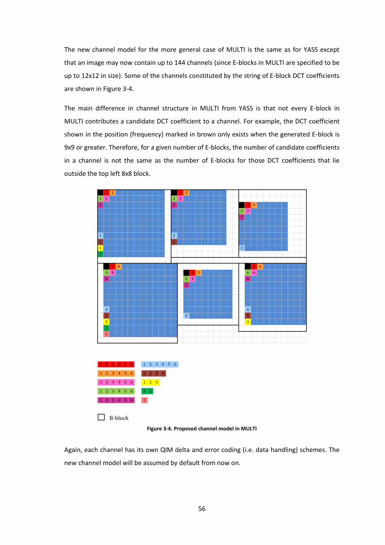
56
The new channel model for the more general case of MULTI is the same as for YASS except
that an image may now contain up to 144 channels (since E-blocks in MULTI are specified to be
up to 12x12 in size). Some of the channels constituted by the string of E-block DCT coefficients
are shown in Figure 3-4.
The main difference in channel structure in MULTI from YASS is that not every E-block in
MULTI contributes a candidate DCT coefficient to a channel. For example, the DCT coefficient
shown in the position (frequency) marked in brown only exists when the generated E-block is
9x9 or greater. Therefore, for a given number of E-blocks, the number of candidate coefficients
in a channel is not the same as the number of E-blocks for those DCT coefficients that lie
outside the top left 8x8 block.
1 1
1 1
1
1
1
1
2 2
2 2
2
2
2
1
1 2 3 4 5 6
1 2 3 4 5 6
1 2 3 4 5 6
1 2 3 4 5 6
1 2 3 4 5 6
3 3
3 3
3
3
4 4
4 4
4
4
3
2
3
1
5 5
5 5
5
5
6 6
6 6
6
6
4
3
1 2 43 65
4321
1 2
1
321
Figure 3-4. Proposed channel model in MULTI
Again, each channel has its own QIM delta and error coding (i.e. data handling) schemes. The
new channel model will be assumed by default from now on.
B-block

57
Now that the channel model has been defined, the specific characteristics of each channel
need to be determined. The rest of the chapter will be concerned with how to determine
relevant channel characteristics and how to use these characteristics to derive data handling
schemes that improve embedding capacity in cell-based stego-systems.
3.2 Coefficient Movement & Previous Delta Values
Although so far the concept of the change in value of data carrying DCT coefficients between
QIM data embedding and retrieval has been referred to, and it has been shown that JPEG
compression is the main factor controlling this change, the exact effects of JPEG compression
have not been discussed. For brevity, the change in value of E-block DCT coefficients between
data embedding and retrieval will be referred to as DCT coefficient movement. When we speak
about movement, we will refer to the absolute value of the change in DCT coefficient value.
Understanding what causes DCT coefficient movement and quantifying how coefficients move
is important in order to gain insight on how to select the best data handling parameters so that
embedding capacity is improved.
This section describes the causes of coefficient movement and presents an analysis of the
characteristics of movement. It also digresses slightly to show a specific case where delta
values have a profound effect on coefficient movement and how this case was used in the
literature to provide delta parameters previously.
3.2.1 Coefficient Movement
So far, the concept that JPEG compression affects E-block DCT coefficients at different
frequencies differently has been referred to, but the amount of error induced in the DCT
coefficients as a result has not be described specifically. This section deals with coefficient
movement more specifically for different cell-based systems.
3.2.1.1 Movement in JPEG-GRID
As a start consider a very extreme cell-based system where the B- and E-blocks coincide at a
size of 8; i.e. B=E=8, shown in Figure 3-5. This is not a practical system but is useful for the
purposes of explaining coefficient movement initially, and will be referred to in this
dissertation as JPEG-GRID. As we will see, the movement in value that a DCT coefficient is likely
to undergo between JPEG compression and de-compression is related to the JPEG quantisation
matrix.
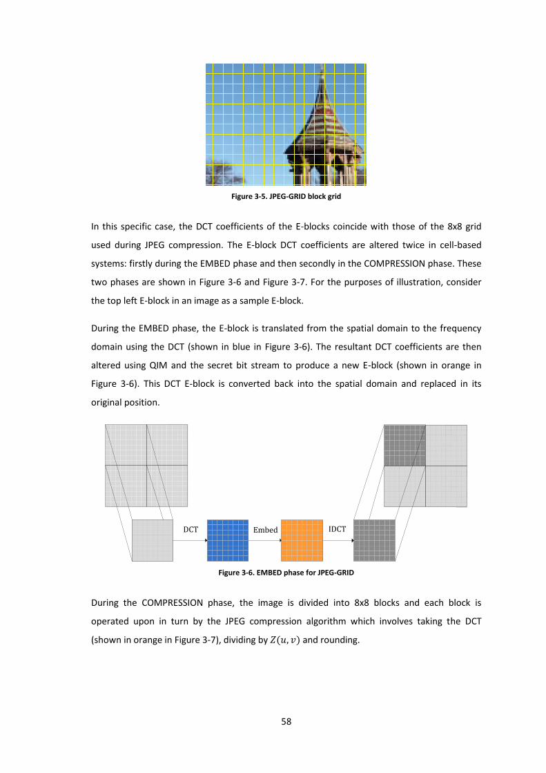
58
Figure 3-5. JPEG-GRID block grid
In this specific case, the DCT coefficients of the E-blocks coincide with those of the 8x8 grid
used during JPEG compression. The E-block DCT coefficients are altered twice in cell-based
systems: firstly during the EMBED phase and then secondly in the COMPRESSION phase. These
two phases are shown in Figure 3-6 and Figure 3-7. For the purposes of illustration, consider
the top left E-block in an image as a sample E-block.
During the EMBED phase, the E-block is translated from the spatial domain to the frequency
domain using the DCT (shown in blue in Figure 3-6). The resultant DCT coefficients are then
altered using QIM and the secret bit stream to produce a new E-block (shown in orange in
Figure 3-6). This DCT E-block is converted back into the spatial domain and replaced in its
original position.
Figure 3-6. EMBED phase for JPEG-GRID
During the COMPRESSION phase, the image is divided into 8x8 blocks and each block is
operated upon in turn by the JPEG compression algorithm which involves taking the DCT
(shown in orange in Figure 3-7), dividing by and rounding.
DCT Embed IDCT
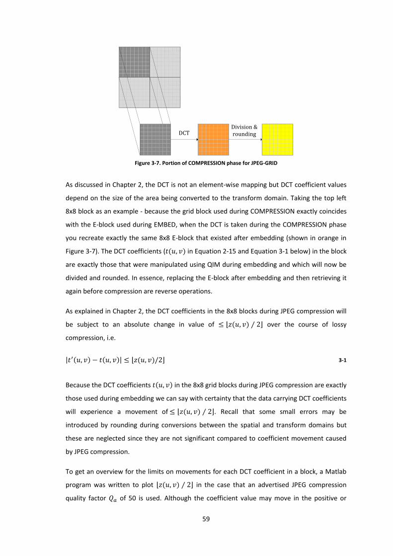
59
Figure 3-7. Portion of COMPRESSION phase for JPEG-GRID
As discussed in Chapter 2, the DCT is not an element-wise mapping but DCT coefficient values
depend on the size of the area being converted to the transform domain. Taking the top left
8x8 block as an example - because the grid block used during COMPRESSION exactly coincides
with the E-block used during EMBED, when the DCT is taken during the COMPRESSION phase
you recreate exactly the same 8x8 E-block that existed after embedding (shown in orange in
Figure 3-7). The DCT coefficients ( in Equation 2-15 and Equation 3-1 below) in the block
are exactly those that were manipulated using QIM during embedding and which will now be
divided and rounded. In essence, replacing the E-block after embedding and then retrieving it
again before compression are reverse operations.
As explained in Chapter 2, the DCT coefficients in the 8x8 blocks during JPEG compression will
be subject to an absolute change in value of ⌊ ⁄ ⌋ over the course of lossy
compression, i.e.
⌊ ⌋ 3-1
Because the DCT coefficients in the 8x8 grid blocks during JPEG compression are exactly
those used during embedding we can say with certainty that the data carrying DCT coefficients
will experience a movement of ⌊ ⁄ ⌋. Recall that some small errors may be
introduced by rounding during conversions between the spatial and transform domains but
these are neglected since they are not significant compared to coefficient movement caused
by JPEG compression.
To get an overview for the limits on movements for each DCT coefficient in a block, a Matlab
program was written to plot ⌊ ⁄ ⌋ in the case that an advertised JPEG compression
quality factor of 50 is used. Although the coefficient value may move in the positive or
DCT Division & rounding
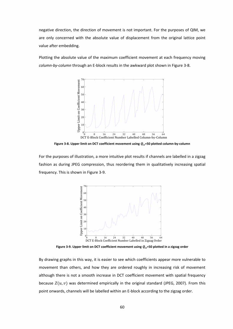
60
negative direction, the direction of movement is not important. For the purposes of QIM, we
are only concerned with the absolute value of displacement from the original lattice point
value after embedding.
Plotting the absolute value of the maximum coefficient movement at each frequency moving
column-by-column through an E-block results in the awkward plot shown in Figure 3-8.
Figure 3-8. Upper limit on DCT coefficient movement using =50 plotted column-by-column
For the purposes of illustration, a more intuitive plot results if channels are labelled in a zigzag
fashion as during JPEG compression, thus reordering them in qualitatively increasing spatial
frequency. This is shown in Figure 3-9.
Figure 3-9. Upper limit on DCT coefficient movement using =50 plotted in a zigzag order
By drawing graphs in this way, it is easier to see which coefficients appear more vulnerable to
movement than others, and how they are ordered roughly in increasing risk of movement
although there is not a smooth increase in DCT coefficient movement with spatial frequency
because was determined empirically in the original standard (JPEG, 2007). From this
point onwards, channels will be labelled within an E-block according to the zigzag order.
0 8 16 24 32 40 48 56 640
10
20
30
40
50
60
70
DCT E-Block Coefficient Number Labelled Column-by-Column
Up
per
Lim
it o
n C
oef
fici
ent
Mo
vem
ent
0 8 16 24 32 40 48 56 640
10
20
30
40
50
60
70
DCT E-Block Coefficient Number Labelled in Zigzag Order
Up
per
Lim
it o
n C
oef
fici
ent
Mo
vem
ent
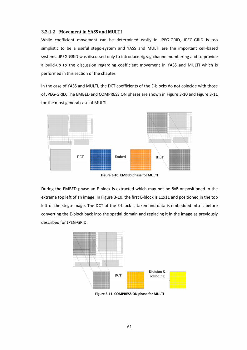
61
3.2.1.2 Movement in YASS and MULTI
While coefficient movement can be determined easily in JPEG-GRID, JPEG-GRID is too
simplistic to be a useful stego-system and YASS and MULTI are the important cell-based
systems. JPEG-GRID was discussed only to introduce zigzag channel numbering and to provide
a build-up to the discussion regarding coefficient movement in YASS and MULTI which is
performed in this section of the chapter.
In the case of YASS and MULTI, the DCT coefficients of the E-blocks do not coincide with those
of JPEG-GRID. The EMBED and COMPRESSION phases are shown in Figure 3-10 and Figure 3-11
for the most general case of MULTI.
Figure 3-10. EMBED phase for MULTI
During the EMBED phase an E-block is extracted which may not be 8x8 or positioned in the
extreme top left of an image. In Figure 3-10, the first E-block is 11x11 and positioned in the top
left of the stego-image. The DCT of the E-block is taken and data is embedded into it before
converting the E-block back into the spatial domain and replacing it in the image as previously
described for JPEG-GRID.
Figure 3-11. COMPRESSION phase for MULTI
DCT Embed IDCT
Division & rounding DCT
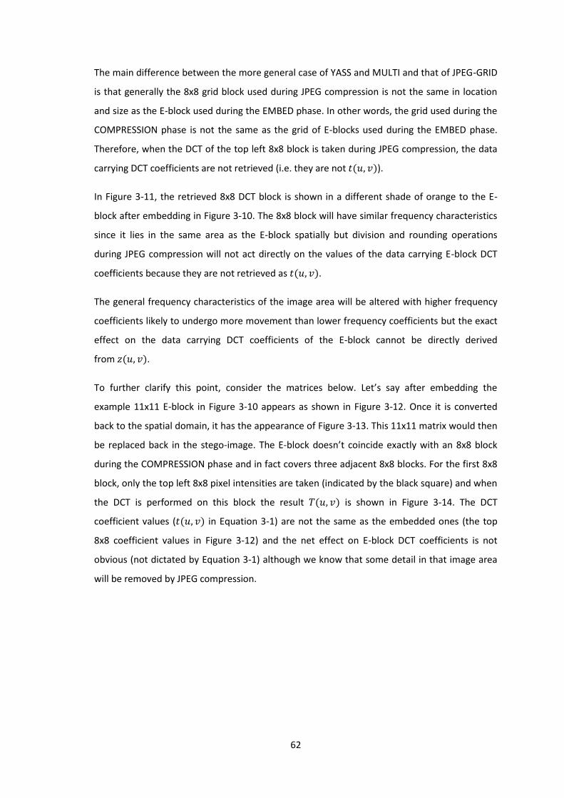
62
The main difference between the more general case of YASS and MULTI and that of JPEG-GRID
is that generally the 8x8 grid block used during JPEG compression is not the same in location
and size as the E-block used during the EMBED phase. In other words, the grid used during the
COMPRESSION phase is not the same as the grid of E-blocks used during the EMBED phase.
Therefore, when the DCT of the top left 8x8 block is taken during JPEG compression, the data
carrying DCT coefficients are not retrieved (i.e. they are not ).
In Figure 3-11, the retrieved 8x8 DCT block is shown in a different shade of orange to the E-
block after embedding in Figure 3-10. The 8x8 block will have similar frequency characteristics
since it lies in the same area as the E-block spatially but division and rounding operations
during JPEG compression will not act directly on the values of the data carrying E-block DCT
coefficients because they are not retrieved as .
The general frequency characteristics of the image area will be altered with higher frequency
coefficients likely to undergo more movement than lower frequency coefficients but the exact
effect on the data carrying DCT coefficients of the E-block cannot be directly derived
from .
To further clarify this point, consider the matrices below. Let’s say after embedding the
example 11x11 E-block in Figure 3-10 appears as shown in Figure 3-12. Once it is converted
back to the spatial domain, it has the appearance of Figure 3-13. This 11x11 matrix would then
be replaced back in the stego-image. The E-block doesn’t coincide exactly with an 8x8 block
during the COMPRESSION phase and in fact covers three adjacent 8x8 blocks. For the first 8x8
block, only the top left 8x8 pixel intensities are taken (indicated by the black square) and when
the DCT is performed on this block the result is shown in Figure 3-14. The DCT
coefficient values ( in Equation 3-1) are not the same as the embedded ones (the top
8x8 coefficient values in Figure 3-12) and the net effect on E-block DCT coefficients is not
obvious (not dictated by Equation 3-1) although we know that some detail in that image area
will be removed by JPEG compression.
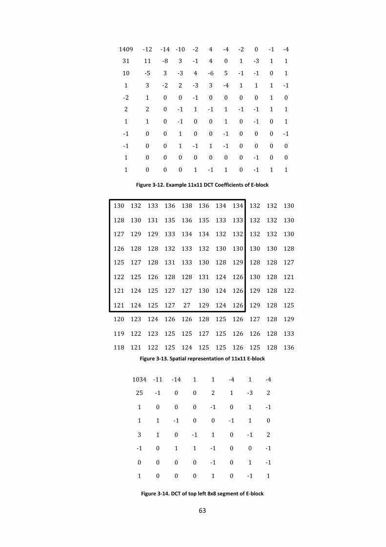
63
1409 -12 -14 -10 -2 4 -4 -2 0 -1 -4
31 11 -8 3 -1 4 0 1 -3 1 1
10 -5 3 -3 4 -6 5 -1 -1 0 1
1 3 -2 2 -3 3 -4 1 1 1 -1
-2 1 0 0 -1 0 0 0 0 1 0
2 2 0 -1 1 -1 1 -1 -1 1 1
1 1 0 -1 0 0 1 0 -1 0 1
-1 0 0 1 0 0 -1 0 0 0 -1
-1 0 0 1 -1 1 -1 0 0 0 0
1 0 0 0 0 0 0 0 -1 0 0
1 0 0 0 1 -1 1 0 -1 1 1
Figure 3-12. Example 11x11 DCT Coefficients of E-block
130 132 133 136 138 136 134 134 132 132 130
128 130 131 135 136 135 133 133 132 132 130
127 129 129 133 134 134 132 132 132 132 130
126 128 128 132 133 132 130 130 130 130 128
125 127 128 131 133 130 128 129 128 128 127
122 125 126 128 128 131 124 126 130 128 121
121 124 125 127 127 130 124 126 129 128 122
121 124 125 127 27 129 124 126 129 128 125
120 123 124 126 126 128 125 126 127 128 129
119 122 123 125 125 127 125 126 126 128 133
118 121 122 125 124 125 125 126 125 128 136
Figure 3-13. Spatial representation of 11x11 E-block
1034 -11 -14 1 1 -4 1 -4
25 -1 0 0 2 1 -3 2
1 0 0 0 -1 0 1 -1
1 1 -1 0 0 -1 1 0
3 1 0 -1 1 0 -1 2
-1 0 1 1 -1 0 0 -1
0 0 0 0 -1 0 1 -1
1 0 0 0 1 0 -1 1
Figure 3-14. DCT of top left 8x8 segment of E-block
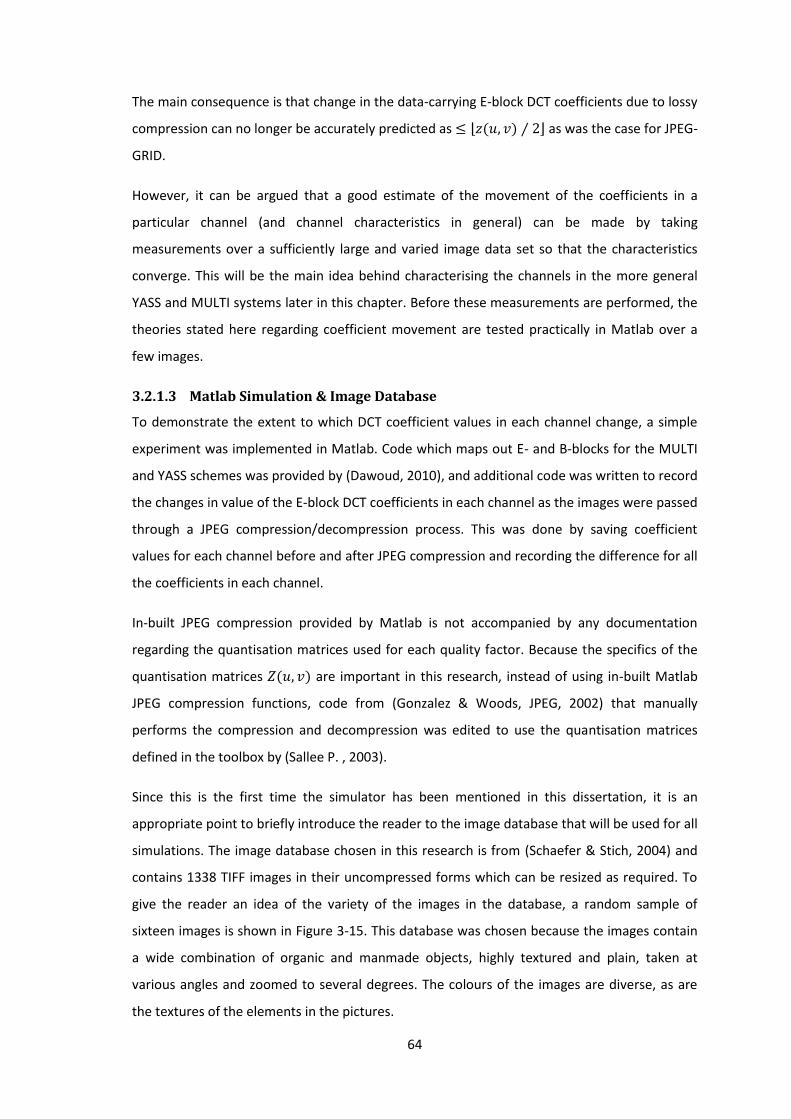
64
The main consequence is that change in the data-carrying E-block DCT coefficients due to lossy
compression can no longer be accurately predicted as ⌊ ⁄ ⌋ as was the case for JPEG-
GRID.
However, it can be argued that a good estimate of the movement of the coefficients in a
particular channel (and channel characteristics in general) can be made by taking
measurements over a sufficiently large and varied image data set so that the characteristics
converge. This will be the main idea behind characterising the channels in the more general
YASS and MULTI systems later in this chapter. Before these measurements are performed, the
theories stated here regarding coefficient movement are tested practically in Matlab over a
few images.
3.2.1.3 Matlab Simulation & Image Database
To demonstrate the extent to which DCT coefficient values in each channel change, a simple
experiment was implemented in Matlab. Code which maps out E- and B-blocks for the MULTI
and YASS schemes was provided by (Dawoud, 2010), and additional code was written to record
the changes in value of the E-block DCT coefficients in each channel as the images were passed
through a JPEG compression/decompression process. This was done by saving coefficient
values for each channel before and after JPEG compression and recording the difference for all
the coefficients in each channel.
In-built JPEG compression provided by Matlab is not accompanied by any documentation
regarding the quantisation matrices used for each quality factor. Because the specifics of the
quantisation matrices are important in this research, instead of using in-built Matlab
JPEG compression functions, code from (Gonzalez & Woods, JPEG, 2002) that manually
performs the compression and decompression was edited to use the quantisation matrices
defined in the toolbox by (Sallee P. , 2003).
Since this is the first time the simulator has been mentioned in this dissertation, it is an
appropriate point to briefly introduce the reader to the image database that will be used for all
simulations. The image database chosen in this research is from (Schaefer & Stich, 2004) and
contains 1338 TIFF images in their uncompressed forms which can be resized as required. To
give the reader an idea of the variety of the images in the database, a random sample of
sixteen images is shown in Figure 3-15. This database was chosen because the images contain
a wide combination of organic and manmade objects, highly textured and plain, taken at
various angles and zoomed to several degrees. The colours of the images are diverse, as are
the textures of the elements in the pictures.
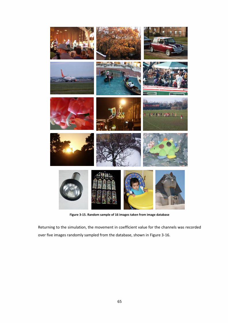
65
Figure 3-15. Random sample of 16 images taken from image database
Returning to the simulation, the movement in coefficient value for the channels was recorded
over five images randomly sampled from the database, shown in Figure 3-16.

66
Figure 3-16. Images used to produce results in Figure 3-18 and Figure 3-19
For these five images, a JPEG quality factor of 80 was used for compression. The corresponding
quantisation matrix from (Sallee P. , 2003) is given in Figure 3-17.
6 4 4 6 10 16 20 24
5 5 6 8 10 23 24 22
6 5 6 10 16 23 28 22
6 7 9 12 20 35 32 25
7 9 15 22 27 44 41 31
10 14 22 26 32 42 45 37
20 26 31 35 41 48 48 40
29 37 38 39 45 40 41 40
Figure 3-17. Quantisation matrix for a quality factor of 80
Using these images, the histograms of DCT coefficient movement for channels 2 and 15 were
plotted (with channels labelled in a zigzag order as explained previously) for JPEG-GRID and
MULTI. for the two channels is highlighted in blue in Figure 3-17. Across the five
images, a total of 7220 E-blocks are created.
The histograms in Figure 3-18 show that the coefficient values for JPEG-GRID in position 2 are
more stable than those in position 15 as expected. In the case of JPEG-GRID, the movement is
also limited to ⌊ ⁄ ⌋ (2 and 5 for channels 2 and 15 respectively). Rarely, movement
of the coefficient is measured as beyond ⌊ ⁄ ⌋ due to rounding errors while converting
between the spatial and transform domains in the EMBED phase but as the histograms show
this is a minor effect.
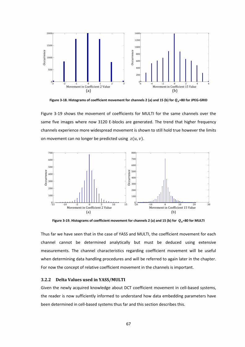
67
Figure 3-18. Histograms of coefficient movement for channels 2 (a) and 15 (b) for =80 for JPEG-GRID
Figure 3-19 shows the movement of coefficients for MULTI for the same channels over the
same five images where now 3120 E-blocks are generated. The trend that higher frequency
channels experience more widespread movement is shown to still hold true however the limits
on movement can no longer be predicted using .
Figure 3-19. Histograms of coefficient movement for channels 2 (a) and 15 (b) for =80 for MULTI
Thus far we have seen that in the case of YASS and MULTI, the coefficient movement for each
channel cannot be determined analytically but must be deduced using extensive
measurements. The channel characteristics regarding coefficient movement will be useful
when determining data handling procedures and will be referred to again later in the chapter.
For now the concept of relative coefficient movement in the channels is important.
3.2.2 Delta Values used in YASS/MULTI
Given the newly acquired knowledge about DCT coefficient movement in cell-based systems,
the reader is now sufficiently informed to understand how data embedding parameters have
been determined in cell-based systems thus far and this section describes this.
-3 -2 -1 0 1 2 30
500
1000
1500
2000
Movement in Coefficient 2 Value
Occ
urr
ence
-6 -4 -2 0 2 4 60
200
400
600
800
1000
1200
1400
Movement in Coefficient 15 Value
Occ
urr
en
ce
(a) (b)
-15 -10 -5 0 5 10 150
100
200
300
400
500
600
700
Movement in Coefficient 2 Value
Occ
urr
ence
-20 -10 0 10 20 300
100
200
300
400
500
600
700
800
Movement in Coefficient 15 Value
Occ
urr
ence
(a) (b)
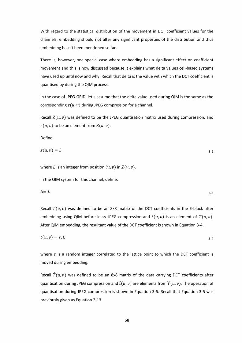
68
With regard to the statistical distribution of the movement in DCT coefficient values for the
channels, embedding should not alter any significant properties of the distribution and thus
embedding hasn’t been mentioned so far.
There is, however, one special case where embedding has a significant effect on coefficient
movement and this is now discussed because it explains what delta values cell-based systems
have used up until now and why. Recall that delta is the value with which the DCT coefficient is
quantised by during the QIM process.
In the case of JPEG-GRID, let’s assume that the delta value used during QIM is the same as the
corresponding during JPEG compression for a channel.
Recall was defined to be the JPEG quantisation matrix used during compression, and
to be an element from .
Define:
3-2
where is an integer from position in .
In the QIM system for this channel, define:
3-3
Recall was defined to be an 8x8 matrix of the DCT coefficients in the E-block after
embedding using QIM before lossy JPEG compression and is an element of .
After QIM embedding, the resultant value of the DCT coefficient is shown in Equation 3-4.
3-4
where is a random integer correlated to the lattice point to which the DCT coefficient is
moved during embedding.
Recall was defined to be an 8x8 matrix of the data carrying DCT coefficients after
quantisation during JPEG compression and are elements from . The operation of
quantisation during JPEG compression is shown in Equation 3-5. Recall that Equation 3-5 was
previously given as Equation 2-13.
69
(
*
3-5
Element-wise, Equation 3-5 can be rewritten as Equation 3-6.
(
* 3-6
By substituting Equation 3-4 in Equation 3-6, you get Equation 3-7.
(
*
3-7
Because the quotient in Equation 3-7 is an integer, there is no rounding and JPEG compression
is no longer lossy.
To see this, consider the step of retrieving the DCT coefficient value during de-compression in
Equation 3-8 where is the recovered DCT coefficient.
3-8
The final effect is:
3-9
This means that if the delta value for a channel is the same as for that channel, then
there should be no errors in the data retrieved since JPEG compression has been made lossless.
The cell-based systems thus far have used JPEG quantisation matrices at different
quality factors as values of delta during QIM. The reasons for this choice are not specified in
the original literature but it is suggested that it was a basic extension of the optimal case just
explained.
As a rough estimate, the delta matrix has a correct look since delta values would be expected
to be larger for higher frequency channels to tolerate more coefficient movement, and as we
have just seen more movement does occur in higher frequency channels. However, there is no
justification for why these values specifically would work well during YASS or MULTI where E-
blocks do not align with grid blocks. MULTI (Dawoud, 2010) crudely extends the JPEG
quantisation matrix to make a 12x12 matrix to accommodate the larger E-block sizes.

70
While using different deltas for DCT coefficients at different frequencies suggests a channel
model as explained earlier in Section 3.1, the literature thus far has not been close to defining
it and error coding has been used across blocks, which has been explained to be inefficient.
In Chapter 2, the term advertised quality factor was used to refer to the factor with which
the quantisation matrix used during JPEG compression is chosen. We now define a second
quality factor - a hiding quality factor as the factor to choose the JPEG quantisation matrix
used to provide delta values for embedding during QIM in YASS and MULTI literature so far.
This chapter will present an approach to choosing delta and error coding schemes more
analytically than done previously.
3.3 Determining Channel Data Handling Parameters Graphically
So far, a new channel model has been deduced and the reasoning for the new channel model
has been validated by exploring more specifically the properties of coefficient movement. It
was stated that the coefficient movement in the more general cases of YASS and MULTI cannot
be derived analytically as in the case of JPEG-GRID, but that through extensive measurements
can be characterised.
We know that we will need to use the channel characteristics somehow with data embedding
and error coding procedures to optimise embedding capacity in each channel but the exact
nature of how to do this has not been explored. Therefore, before acquiring the channel
characteristics, it is worth taking a step back and getting an overview of how we will be able to
combine channel characteristics with our understanding of data handling procedures to derive
better data handling parameters that will hopefully address the relatively low embedding
capacity of cell-based systems (in effect the main research problem statement in this
dissertation).
The main players in embedding capacity are selection criteria and error coding which are both
connected to the value of QIM delta. This section discusses these broad issues.
If error coding is ignored for the moment, the effect of the choice of delta on error in a channel
can be explained. Consider the histogram of movement in channel 15 in JPEG-GRID for a JPEG
quality factor of 80 taken from Figure 3-18(b), repeated in Figure 3-20. Assuming as an
example the use of a delta of 10 for this channel, tolerance boundaries representing the limit
on coefficient movement for correct data retrieval ( ⁄ ) can be superimposed on this
histogram as shown.
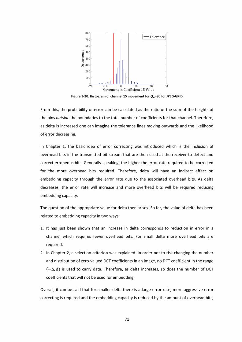
71
Figure 3-20. Histogram of channel 15 movement for =80 for JPEG-GRID
From this, the probability of error can be calculated as the ratio of the sum of the heights of
the bins outside the boundaries to the total number of coefficients for that channel. Therefore,
as delta is increased one can imagine the tolerance lines moving outwards and the likelihood
of error decreasing.
In Chapter 1, the basic idea of error correcting was introduced which is the inclusion of
overhead bits in the transmitted bit stream that are then used at the receiver to detect and
correct erroneous bits. Generally speaking, the higher the error rate required to be corrected
for the more overhead bits required. Therefore, delta will have an indirect effect on
embedding capacity through the error rate due to the associated overhead bits. As delta
decreases, the error rate will increase and more overhead bits will be required reducing
embedding capacity.
The question of the appropriate value for delta then arises. So far, the value of delta has been
related to embedding capacity in two ways:
1. It has just been shown that an increase in delta corresponds to reduction in error in a
channel which requires fewer overhead bits. For small delta more overhead bits are
required.
2. In Chapter 2, a selection criterion was explained. In order not to risk changing the number
and distribution of zero-valued DCT coefficients in an image, no DCT coefficient in the range
is used to carry data. Therefore, as delta increases, so does the number of DCT
coefficients that will not be used for embedding.
Overall, it can be said that for smaller delta there is a large error rate, more aggressive error
correcting is required and the embedding capacity is reduced by the amount of overhead bits,
-20 -10 0 10 20 300
100
200
300
400
500
600
700
800
Movement in Coefficient 15 Value
Occ
urr
ence
Tolerance
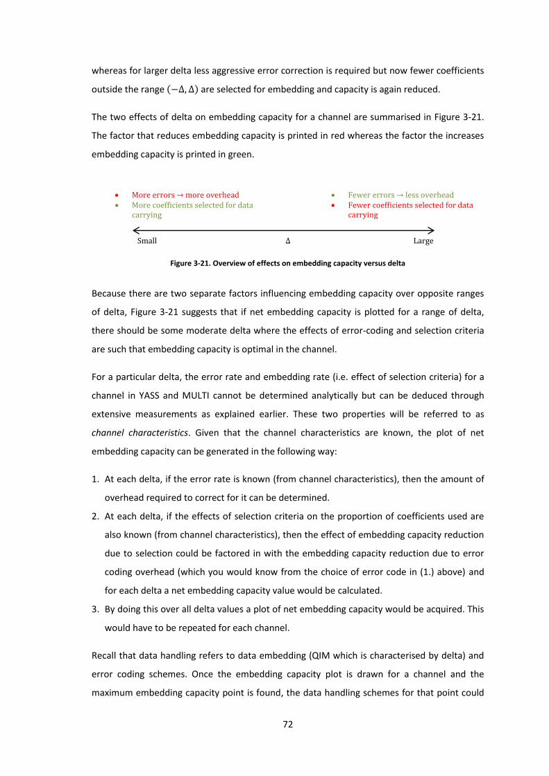
72
whereas for larger delta less aggressive error correction is required but now fewer coefficients
outside the range are selected for embedding and capacity is again reduced.
The two effects of delta on embedding capacity for a channel are summarised in Figure 3-21.
The factor that reduces embedding capacity is printed in red whereas the factor the increases
embedding capacity is printed in green.
Figure 3-21. Overview of effects on embedding capacity versus delta
Because there are two separate factors influencing embedding capacity over opposite ranges
of delta, Figure 3-21 suggests that if net embedding capacity is plotted for a range of delta,
there should be some moderate delta where the effects of error-coding and selection criteria
are such that embedding capacity is optimal in the channel.
For a particular delta, the error rate and embedding rate (i.e. effect of selection criteria) for a
channel in YASS and MULTI cannot be determined analytically but can be deduced through
extensive measurements as explained earlier. These two properties will be referred to as
channel characteristics. Given that the channel characteristics are known, the plot of net
embedding capacity can be generated in the following way:
1. At each delta, if the error rate is known (from channel characteristics), then the amount of
overhead required to correct for it can be determined.
2. At each delta, if the effects of selection criteria on the proportion of coefficients used are
also known (from channel characteristics), then the effect of embedding capacity reduction
due to selection could be factored in with the embedding capacity reduction due to error
coding overhead (which you would know from the choice of error code in (1.) above) and
for each delta a net embedding capacity value would be calculated.
3. By doing this over all delta values a plot of net embedding capacity would be acquired. This
would have to be repeated for each channel.
Recall that data handling refers to data embedding (QIM which is characterised by delta) and
error coding schemes. Once the embedding capacity plot is drawn for a channel and the
maximum embedding capacity point is found, the data handling schemes for that point could
Δ Large Small
More errors → more overhead More coefficients selected for data
carrying
Fewer errors → less overhead Fewer coefficients selected for data
carrying

73
be deduced by reading the QIM delta value off of the x-axis and determining the error coding
scheme that was implemented at the maximum capacity point.
It can now be seen that this type of plot holds the key to deriving optimal data handling
schemes for a channel and the focus of this work now shifts to determining this type of plot for
the defined channels.
One final factor related to delta not yet mentioned but worth consideration is that the larger
the delta, the greater the embedding artefacts which may increase detectability. In cell-based
systems, the random nature of embedding is the most important aspect in ensuring security
therefore it is assumed for now that the random nature of embedding should guarantee
adequate resistance against steganalysis even if the delta values for the channels deduced
here are higher than those in the literature previously. It is expected, however, that the delta
values derived here will be similar to existing ones. This assumption will be tested in Chapter 4.
Now that we have a global view of what is required to find data handling parameters for each
channel, the rest of this chapter deals with deducing channel characteristics and consolidating
them with error coding systems to give this net embedding capacity plot and hence deriving
data handling schemes.
3.4 Channel Characterisation
In order to plot the net embedding capacity curve, first the channels in YASS and MULTI need
to be characterised which can only be done empirically through extensive measurements.
Specifically, the error rate and effects of selection criteria (embedding rate) for each delta for
each channel need to be determined. This section formally defines the channel characteristics
of interest and how the measurements are conducted, as well as presents some final channel
characteristics and comments.
3.4.1 Determining Channel Characteristics Empirically
In order to plot net embedding capacity versus delta, the characteristics of the channels need
to be known first. The idea here is to gather statistics of the channel for each delta regarding
the proportion of channel coefficients that meet selection criteria and the error rate a
correction code would be required to cater for. For the moment, we ignore error coding
requirements.
It has already been seen that the DCT coefficients in the E-blocks of MULTI and YASS are not
directly correlated to the JPEG quantisation matrix values as in the case of JPEG-GRID.
To solve this problem, an assumption is made that if channel characteristics are measured over
74
a sufficiently large and variable set of images for the most general case of MULTI until the
characteristics converge, the characteristics will be a good representation of the channel
properties in any image likely to be used as a cover image.
The channel characteristics deduced in this section will be for the 144 channels in the MULTI
system. These characteristics will be representative of all cell-based systems since they all
generate E-blocks randomly in an image. Statistically speaking, the only real difference then
between YASS and MULTI is the number of channels, but the channels in the top left 8x8
segment of the MULTI E-blocks will have the same statistical properties as those of YASS E-
blocks. All of the AC channels are considered for data carrying and not only the first 19 as
originally presented in the literature.
In order to plot the embedding capacity against delta, for each value of delta the proportion of
DCT coefficients in the channel that meet selection criteria needs to be known, and the error
rate needs to be known so that the amount of overhead related to coding can be found.
Although already introduced, these two critical characterising factors for a channel are defined
formally next.
i. Embedding Rate
The average embedding rate for a block of data bits is defined in Equation 3-10.
3-10
The embedding rate represents the proportion of the candidate coefficients in each channel
that are deemed acceptable to carry information by selection criteria. Taken as an average
over a channel, it also represents how appropriate a particular channel is to carry data with
regard to the security of the system.
ii. Error Rate
The average error rate for a block of data bits is defined in Equation 3-11.
3-11
The error rate represents the likelihood of error in a particular group of embedded message
bits, based on some observed input and output bit stream. More specifically, given the
selection criteria, the error rate indicates the extent to which the surviving coefficients are
75
appropriate for data embedding for a given delta and advertised quality factor used for
JPEG compression of the stego-image.
To measure these rates, a large image database and simulator are required. The simulator
should, for each image, and for each delta for each channel, determine the embedding rate
and error rate using the MULTI system.
The image database has already been introduced in Section 3.2.1.3 and the simulator was
implemented in Matlab. While the code received from (Dawoud, 2010) generated the E- and
B- blocks in an image for YASS and MULTI, there was no functionality accommodating a
channel model such as the one presented here since this is original to this dissertation. Recall
that the module recording movement in E-block DCT coefficient values between before and
after JPEG compression was added on previously. Some pertinent elements of the simulator
and further modules added onto it at this point are:
The original code of (Dawoud, 2010) allowed for pseudo-random data bits to be embedded
into the E-block DCT coefficients. This is a good approximation for the nature of the data a
steganographer would embed since the data is likely to have undergone cryptographic
scrambling and error correcting coding.
The number of bits embedded into each channel corresponds to the number of DCT
coefficients used for data carrying in a channel after selection criteria and the required
number of data bits can only be determined once the embedding rate is known. To
determine this number, an image undergoes a preliminary stage of processing before data
generation and embedding.
The code of (Dawoud, 2010) only implemented LSB embedding. The code was extended to
perform QIM embedding at the transmitter side and QIM de-embedding at the receiver
side with a different delta specified for each channel.
The code of (Dawoud, 2010) embedded data for the purposes of generating stego-images
that could be visually and statistically analysed. Modules were added to record the input
and retrieved secret message bit streams for each channel used to analyse the error rate
and distribution of errors in a channel.

76
Before acquiring channel characteristics, the advertised JPEG compression quality factor
must be decided upon for 2 reasons:
The greater the amount of compression, the more likely the movement in the E-block DCT
coefficient due to the compression process and this effects all of the parameters for data
embedding and error correcting.
In the eyes of a steganalyser, it cannot distinguish between distortion due to the
embedding process or due to heavy quantisation of the JPEG compression process.
Therefore, a more heavily compressed image containing data will be more resistant to
steganalysis than a stego-image that is more lightly compressed.
All other literature on cell-based systems uses =75 and to conform to this 75 is also used
here.
There is also a more subtle point to be made regarding measurement of the error and
embedding rates. In communication channels, the characteristics of a channel can be
measured over some time in batches. Given a time segment, there will be certain statistics
regarding the behaviour of the channel determined from previous observations. In
characterising the channels in cell-based stego-systems, it has already been explained that a
time base is not used, but rather the bits are embedded spatially. In the same way that a signal
can be analysed over a specific time segment, we need to examine the channel over a certain
number (batch) of coefficients (each coefficient retrieved from an E-block in sequence as
shown in Figure 3-4).
The number of coefficients in a batch depends on the accuracy with which the embedding and
error rates are required to be measured. If we take the batch to be one coefficient, then at any
time the channel can have either 0% or 100% embedding or error rates which is not a realistic
measurement because this case is so limited. As the number of coefficients in a batch is
increased, the accuracy with which we can record the rates increases. Using a batch of 100
coefficients, we can get accuracy in rates of up to 1% which suffices for this application.
To summarise then, the specifics of acquiring error and embedding rate statistics with regard
to these batches (accommodated by the above-stated simulator properties) are:
1. Divide the channel coefficients into batches of 100 (ignore any residual coefficients after
batching).
2. For each batch: Check how many meet selection criteria based on the delta value for that
channel. This proportion is noted as an embedding rate measurement.
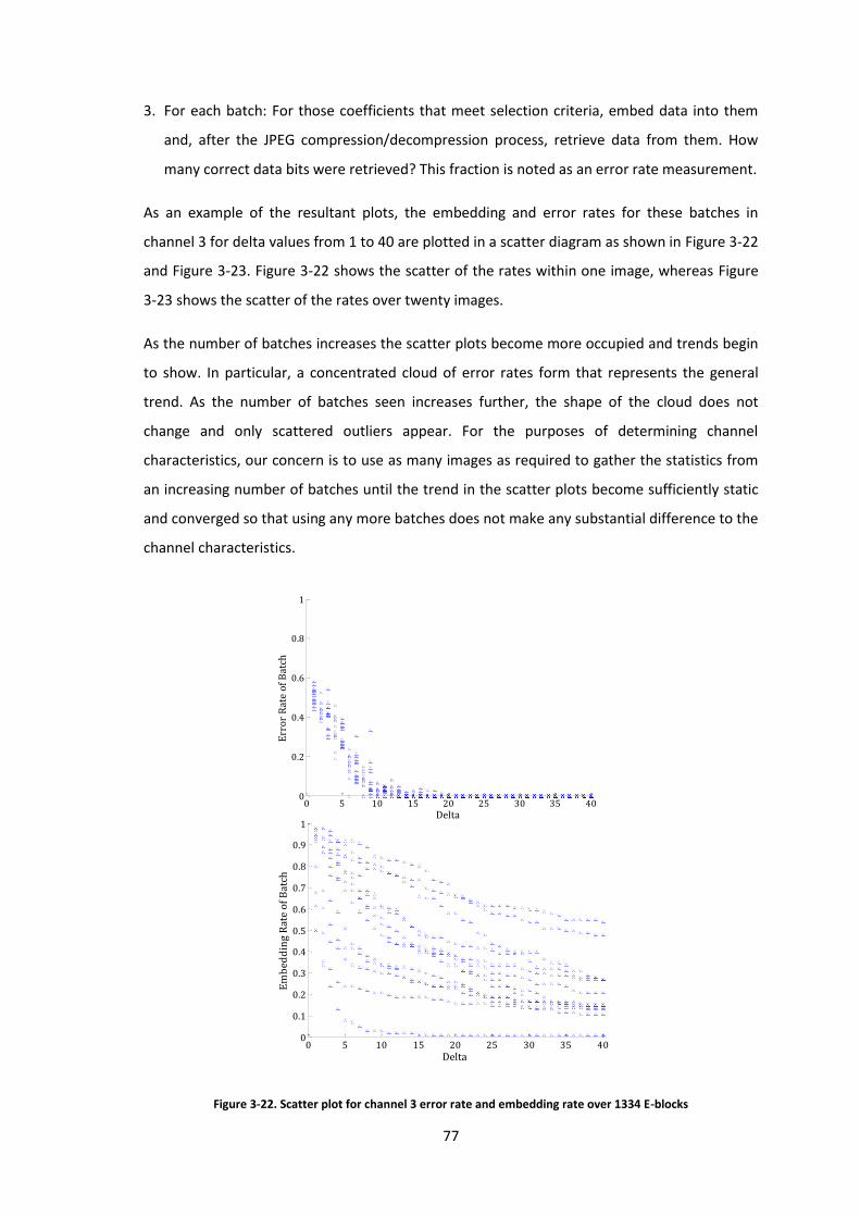
77
3. For each batch: For those coefficients that meet selection criteria, embed data into them
and, after the JPEG compression/decompression process, retrieve data from them. How
many correct data bits were retrieved? This fraction is noted as an error rate measurement.
As an example of the resultant plots, the embedding and error rates for these batches in
channel 3 for delta values from 1 to 40 are plotted in a scatter diagram as shown in Figure 3-22
and Figure 3-23. Figure 3-22 shows the scatter of the rates within one image, whereas Figure
3-23 shows the scatter of the rates over twenty images.
As the number of batches increases the scatter plots become more occupied and trends begin
to show. In particular, a concentrated cloud of error rates form that represents the general
trend. As the number of batches seen increases further, the shape of the cloud does not
change and only scattered outliers appear. For the purposes of determining channel
characteristics, our concern is to use as many images as required to gather the statistics from
an increasing number of batches until the trend in the scatter plots become sufficiently static
and converged so that using any more batches does not make any substantial difference to the
channel characteristics.
Figure 3-22. Scatter plot for channel 3 error rate and embedding rate over 1334 E-blocks
0 5 10 15 20 25 30 35 400
0.2
0.4
0.6
0.8
1
Delta
Err
or
Rat
e o
f B
atch
0 5 10 15 20 25 30 35 400
0.1
0.2
0.3
0.4
0.5
0.6
0.7
0.8
0.9
1
Delta
Em
bed
din
g R
ate
of
Bat
ch
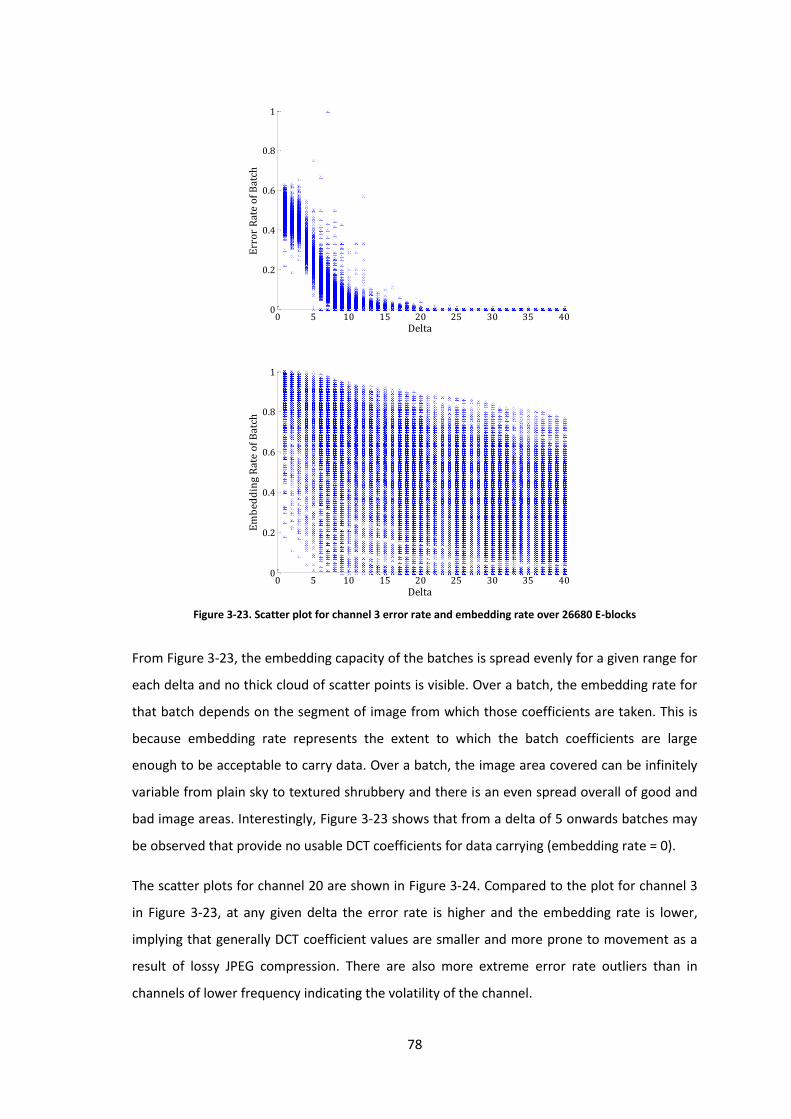
78
Figure 3-23. Scatter plot for channel 3 error rate and embedding rate over 26680 E-blocks
From Figure 3-23, the embedding capacity of the batches is spread evenly for a given range for
each delta and no thick cloud of scatter points is visible. Over a batch, the embedding rate for
that batch depends on the segment of image from which those coefficients are taken. This is
because embedding rate represents the extent to which the batch coefficients are large
enough to be acceptable to carry data. Over a batch, the image area covered can be infinitely
variable from plain sky to textured shrubbery and there is an even spread overall of good and
bad image areas. Interestingly, Figure 3-23 shows that from a delta of 5 onwards batches may
be observed that provide no usable DCT coefficients for data carrying (embedding rate = 0).
The scatter plots for channel 20 are shown in Figure 3-24. Compared to the plot for channel 3
in Figure 3-23, at any given delta the error rate is higher and the embedding rate is lower,
implying that generally DCT coefficient values are smaller and more prone to movement as a
result of lossy JPEG compression. There are also more extreme error rate outliers than in
channels of lower frequency indicating the volatility of the channel.
0 5 10 15 20 25 30 35 400
0.2
0.4
0.6
0.8
1
Delta
Err
or
Rat
e o
f B
atch
0 5 10 15 20 25 30 35 400
0.2
0.4
0.6
0.8
1
Delta
Em
bed
din
g R
ate
of
Bat
ch
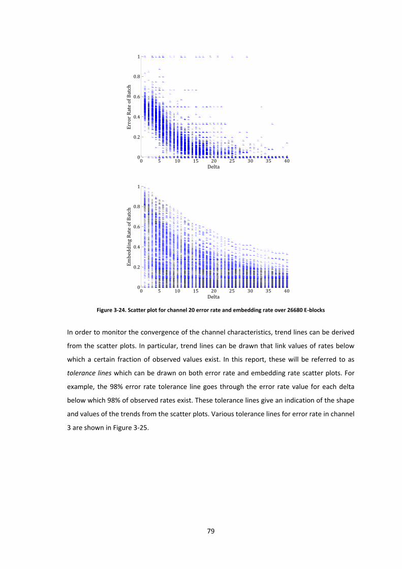
79
Figure 3-24. Scatter plot for channel 20 error rate and embedding rate over 26680 E-blocks
In order to monitor the convergence of the channel characteristics, trend lines can be derived
from the scatter plots. In particular, trend lines can be drawn that link values of rates below
which a certain fraction of observed values exist. In this report, these will be referred to as
tolerance lines which can be drawn on both error rate and embedding rate scatter plots. For
example, the 98% error rate tolerance line goes through the error rate value for each delta
below which 98% of observed rates exist. These tolerance lines give an indication of the shape
and values of the trends from the scatter plots. Various tolerance lines for error rate in channel
3 are shown in Figure 3-25.
0 5 10 15 20 25 30 35 400
0.2
0.4
0.6
0.8
1
Delta
Em
bed
din
g R
ate
of
Bat
ch
0 5 10 15 20 25 30 35 400
0.2
0.4
0.6
0.8
1
Delta
Err
or
Rat
e o
f B
atch
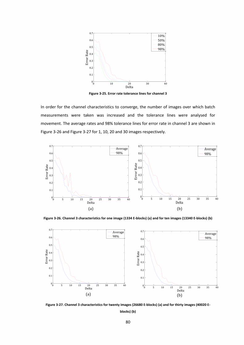
80
Figure 3-25. Error rate tolerance lines for channel 3
In order for the channel characteristics to converge, the number of images over which batch
measurements were taken was increased and the tolerance lines were analysed for
movement. The average rates and 98% tolerance lines for error rate in channel 3 are shown in
Figure 3-26 and Figure 3-27 for 1, 10, 20 and 30 images respectively.
Figure 3-26. Channel 3 characteristics for one image (1334 E-blocks) (a) and for ten images (13340 E-blocks) (b)
Figure 3-27. Channel 3 characteristics for twenty images (26680 E-blocks) (a) and for thirty images (40020 E-
blocks) (b)
0 10 20 30 400
0.1
0.2
0.3
0.4
0.5
0.6
0.7
Err
or
Rat
eDelta
10%
50%
80%
98%
0 5 10 15 20 25 30 35 400
0.1
0.2
0.3
0.4
0.5
0.6
0.7
Err
or
Rat
e
Delta
Average
98%
(a)
0 5 10 15 20 25 30 35 400
0.1
0.2
0.3
0.4
0.5
0.6
0.7
Err
or
Ra
te
Delta
Average
98%
(b)
0 5 10 15 20 25 30 35 400
0.1
0.2
0.3
0.4
0.5
0.6
0.7
Err
or
Rat
e
Delta
Average
98%
(a) (b)
0 5 10 15 20 25 30 35 400
0.1
0.2
0.3
0.4
0.5
0.6
0.7
Err
or
Rat
e
Delta
Average
98%
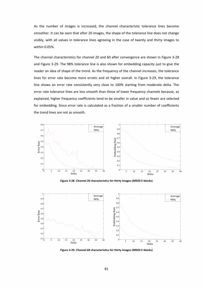
81
As the number of images is increased, the channel characteristic tolerance lines become
smoother. It can be seen that after 20 images, the shape of the tolerance line does not change
visibly, with all values in tolerance lines agreeing in the case of twenty and thirty images to
within 0.05%.
The channel characteristics for channel 20 and 60 after convergence are shown in Figure 3-28
and Figure 3-29. The 98% tolerance line is also shown for embedding capacity just to give the
reader an idea of shape of the trend. As the frequency of the channel increases, the tolerance
lines for error rate become more erratic and sit higher overall. In Figure 3-29, the tolerance
line shows an error rate consistently very close to 100% starting from moderate delta. The
error rate tolerance lines are less smooth than those of lower frequency channels because, as
explained, higher frequency coefficients tend to be smaller in value and so fewer are selected
for embedding. Since error rate is calculated as a fraction of a smaller number of coefficients
the trend lines are not as smooth.
Figure 3-28. Channel 20 characteristics for thirty images (40020 E-blocks)
Figure 3-29. Channel 60 characteristics for thirty images (40020 E-blocks)
0 5 10 15 20 25 30 35 400
0.1
0.2
0.3
0.4
0.5
0.6
0.7
0.8
Err
or
Rat
e
Delta
Average
98%
5 10 15 20 25 30 35 400
0.1
0.2
0.3
0.4
0.5
0.6
0.7
0.8
0.9
1
Delta
Em
bed
din
g R
ate
Average
98%
0 5 10 15 20 25 30 35 400.1
0.2
0.3
0.4
0.5
0.6
0.7
0.8
0.9
1
Err
or
Rat
e
Delta
Average
98%
5 10 15 20 25 30 35 400
0.1
0.2
0.3
0.4
0.5
0.6
0.7
0.8
0.9
1
Delta
Em
bed
din
g R
ate
Average
98%
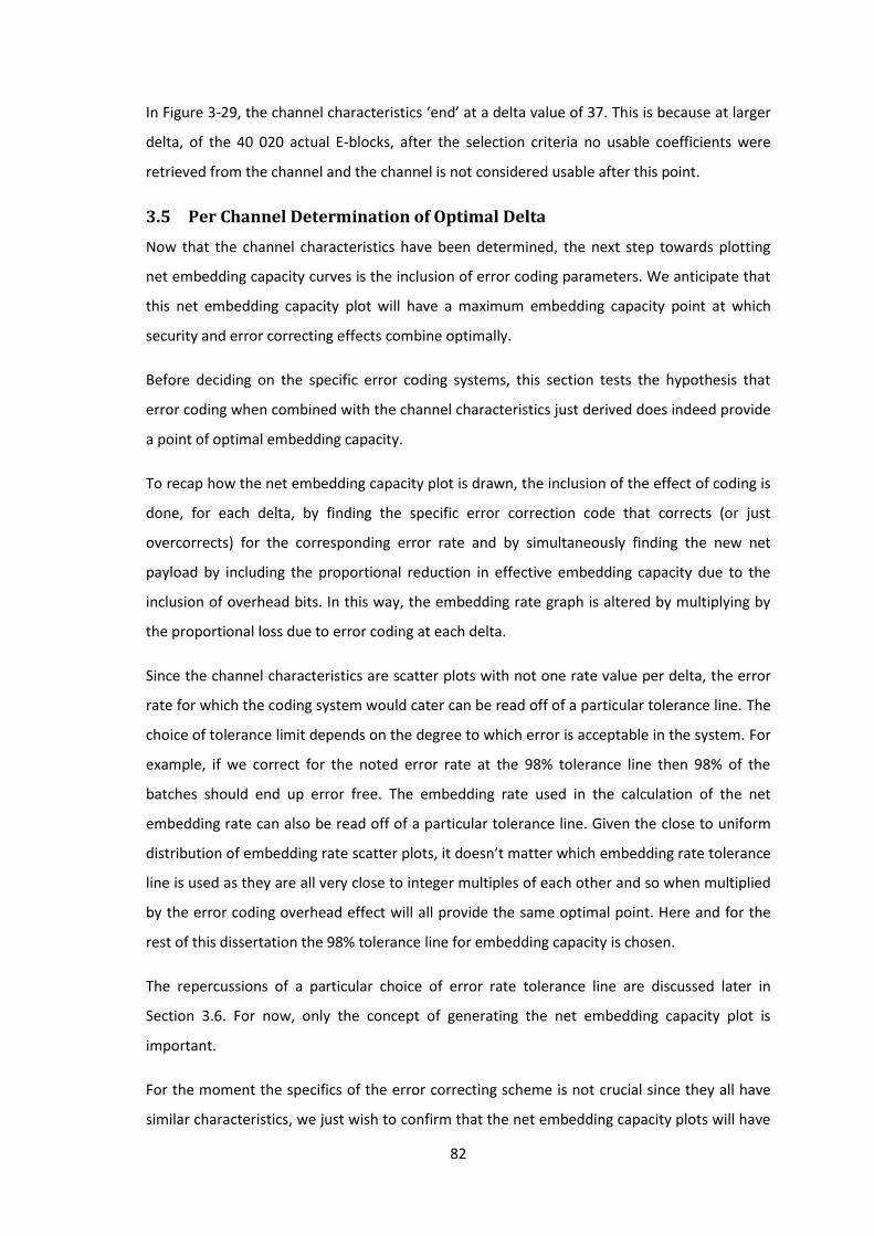
82
In Figure 3-29, the channel characteristics ‘end’ at a delta value of 37. This is because at larger
delta, of the 40 020 actual E-blocks, after the selection criteria no usable coefficients were
retrieved from the channel and the channel is not considered usable after this point.
3.5 Per Channel Determination of Optimal Delta
Now that the channel characteristics have been determined, the next step towards plotting
net embedding capacity curves is the inclusion of error coding parameters. We anticipate that
this net embedding capacity plot will have a maximum embedding capacity point at which
security and error correcting effects combine optimally.
Before deciding on the specific error coding systems, this section tests the hypothesis that
error coding when combined with the channel characteristics just derived does indeed provide
a point of optimal embedding capacity.
To recap how the net embedding capacity plot is drawn, the inclusion of the effect of coding is
done, for each delta, by finding the specific error correction code that corrects (or just
overcorrects) for the corresponding error rate and by simultaneously finding the new net
payload by including the proportional reduction in effective embedding capacity due to the
inclusion of overhead bits. In this way, the embedding rate graph is altered by multiplying by
the proportional loss due to error coding at each delta.
Since the channel characteristics are scatter plots with not one rate value per delta, the error
rate for which the coding system would cater can be read off of a particular tolerance line. The
choice of tolerance limit depends on the degree to which error is acceptable in the system. For
example, if we correct for the noted error rate at the 98% tolerance line then 98% of the
batches should end up error free. The embedding rate used in the calculation of the net
embedding rate can also be read off of a particular tolerance line. Given the close to uniform
distribution of embedding rate scatter plots, it doesn’t matter which embedding rate tolerance
line is used as they are all very close to integer multiples of each other and so when multiplied
by the error coding overhead effect will all provide the same optimal point. Here and for the
rest of this dissertation the 98% tolerance line for embedding capacity is chosen.
The repercussions of a particular choice of error rate tolerance line are discussed later in
Section 3.6. For now, only the concept of generating the net embedding capacity plot is
important.
For the moment the specifics of the error correcting scheme is not crucial since they all have
similar characteristics, we just wish to confirm that the net embedding capacity plots will have
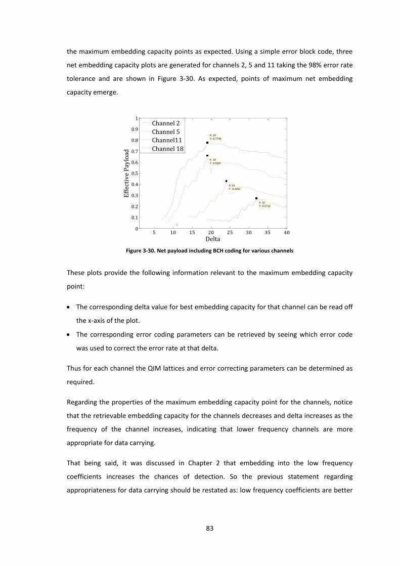
83
the maximum embedding capacity points as expected. Using a simple error block code, three
net embedding capacity plots are generated for channels 2, 5 and 11 taking the 98% error rate
tolerance and are shown in Figure 3-30. As expected, points of maximum net embedding
capacity emerge.
Figure 3-30. Net payload including BCH coding for various channels
These plots provide the following information relevant to the maximum embedding capacity
point:
The corresponding delta value for best embedding capacity for that channel can be read off
the x-axis of the plot.
The corresponding error coding parameters can be retrieved by seeing which error code
was used to correct the error rate at that delta.
Thus for each channel the QIM lattices and error correcting parameters can be determined as
required.
Regarding the properties of the maximum embedding capacity point for the channels, notice
that the retrievable embedding capacity for the channels decreases and delta increases as the
frequency of the channel increases, indicating that lower frequency channels are more
appropriate for data carrying.
That being said, it was discussed in Chapter 2 that embedding into the low frequency
coefficients increases the chances of detection. So the previous statement regarding
appropriateness for data carrying should be restated as: low frequency coefficients are better
5 10 15 20 25 30 35 400
0.1
0.2
0.3
0.4
0.5
0.6
0.7
0.8
0.9
1
X: 19
Y: 0.7749
Eff
ecti
ve
Pay
load
Delta
X: 19
Y: 0.6587
X: 24
Y: 0.4262
X: 32
Y: 0.2712
Channel 2
Channel 5
Channel11
Channel 18

84
for data carrying in terms of the amount of data they can carry provided that the value of delta
isn’t so large that a steganalyser can detect the embedding artefacts.
It is assumed that the random nature of embedding in itself will secure resistance to
steganalysis even if the values of delta for lower frequency channels are determined to be
slightly higher than those used in the quantisation matrix for hiding quality factor . This will
be assumed for now and checked in Chapter 4 where performance of the determined system
is examined.
3.6 Compensation for Errors
Now that channel characteristics have been determined and that it has been confirmed that
consolidating channel characteristics with error coding parameters does provide data
embedding and error coding parameters that give optimal embedding capacity, the exact
nature of the error coding scheme to be implemented needs to be discussed and once this has
been decided, similar plots as shown in Figure 3-30 can be deduced which, with some
reasoning, should provide a solution.
Previous literature on cell-based systems has used RA coding. In terms of embedding capacity
RA coding is inefficient because of the high number of redundant bits. This section works on
the premise that a better coding system can be found. A comparison between the
performances of the new system versus the old one is then provided in Chapter 4.
It should be mentioned that, depending on the application, errors may be allowed in a secret
message. For example, if the message is text or voice, then corruption of some letters or
distortion in the voice probably won’t prevent the receiver from understanding what was
meant. However, if the secret message data is a bank balance, then the movement of a
decimal place will have a dramatic impact on how the retrieved message is interpreted by the
intended recipient. In this dissertation, no strict limitations are placed on application and it is
assumed that the designer would want as close to error-free transmission as possible to satisfy
the more strict case. Also, should an error occur, there should be a mechanism in place so that
the recipient will realise this and request a re-transmission if desired and possible.
3.6.1 Error Correction Selection
Given a channel subject to errors, error coding can be approached in a few ways. The one way
is to not perform error correction but only perform the significantly simpler task of error
detection. Should an error be detected at the receiver, a request is sent using a feedback
channel to the transmitter to re-transmit the data in a different cover image. This is not
85
practical in stego-systems because there is no intuitive feedback channel and the requirement
that the transmitter regularly re-transmit messages could arouse suspicion from a warden.
A more practical approach is the use of forward error correcting (FEC) codes. In this scheme,
redundancy is introduced by interleaving the data to be transmitted with check bits (overhead)
that are used at the receiver to correct errors. Initially, FEC codes were unpopular due to their
high complexity, but since this is now less of a problem following the development of many
powerful electronic systems, the effectiveness often outweighs other schemes.
The choice of FEC code is governed by three factors:
The nature of the errors (i.e. random or burst).
The degree to which the errors occur.
In the case of random errors, it is assumed that each bit has the same likelihood of error,
independent of any other bits, and so the average error rate represents the likelihood of
any bit being in error at any time. In the case of burst errors, the longest burst expected in
the channel needs to be quantised.
Whether the length of data to be transmitted is known in advance and can be broken down
into blocks, or whether a continuous stream of data of unknown length needs to be
accommodated.
A reasonable cover image will contain regions of varying texture and suitability to carry data.
Consider the simple case where a message is hidden in channel coefficients sequentially in
adjacent E-blocks as shown in Figure 3-3 and Figure 3-4; if there happens to be an image
region that is particularly error-prone then a substantial burst of error will occur. Due to the
massive variety in image content, it would be difficult to predict the extent of the error
burstiness. This problem can be avoided by embedding data in a pseudo-random order around
an image rather than sequentially in adjacent E-blocks. By doing this, the probabilities of
adjacent data bits being in error are decorrelated and the nature of the error becomes random
(Vaudenay, 2002). The statistics relating to this type of error can be derived directly from the
error rate tolerance lines of the channel error characteristics. The scattering of data around
the image can be done simply using a pseudo-random number generator, the key to which can
be shared in the stego-key.
Given that the purpose of this work is to improve embedding capacity, we will narrow our
focus of error correcting schemes to moderate ones that correct for small to moderate
amounts of error and which have minimal overhead. Correcting for channels and delta values
86
with very high error rates is possible with aggressive coding schemes, but goes against the
main goal of this work since the heavy overhead requirements would offset any benefit of
using the channel to contribute substantially to net embedding capacity.
Within the field of light random error correcting coding, the two primary candidates are
convolutional codes and Bose, Chaudhuri and Hocquenghem (BCH) codes (Lin & Costello,
1983). BCH codes are a type of block code that divide the input bit stream into blocks of fixed
size that are then padded with overhead parity bits mapping an input block into a code word.
Convolutional codes also convert the input message stream into code words, but do not divide
the stream into blocks. Rather, it outputs a code word based on a set of current input bits and
previous input bits stored in memory. Convolutional codes are used in real-time applications
when the length of the input stream is not known prior to encoding. With regard to stego-
systems, there is no reason why the cover image and input bit streams would not be known in
advance, making the system more suitable for BCH codes.
BCH codes are a popular generalisation of the well-known Hamming codes. They are highly
flexible, allowing variation in block size and overhead within certain error thresholds and
mathematical constraints.
As defined in (Lin & Costello, 1983):
Given any positive integers and , with and , there exists a binary BCH
code with the following parameters:
3-12
3-13
3-14
where represents the number of errors that can be corrected, represents the length of the
final codeword and represents the size of the input block of message bits. A table
documenting values of that exist can be found in (Proakis & Salehi, 2002). The possible
values of are 7, 15, 31, 63, 127, 255, 511 and 1023. For a given error rate, a BCH code with
smaller block length has a better code rate ( ⁄ ). BCH codes can correct for errors up to
approximately 25% of the entire block (including overhead bits).
87
A disadvantage in using BCH codes is that some bits may need to be rejected after blocking if
the number of coefficients in a channel is not an integer multiple of , with an average ⁄
bits being lost per channel. However, the simplicity and effectiveness of the codes combined
with the likelihood that proportionally only a small number of bits will be lost makes BCH
codes a good choice.
With regard to the simulator, further modules were added at the front and back ends to
provide BCH encoding before embedding and decoding after retrieval. The front end is shown
in Figure 3-31. Given an initial secret message bit stream (110010100001101…), each channel
has capacity to carry bits after selection criteria (determined using a preliminary stage in
the Matlab simulator as explained in Section 3.4.1). Recall channel 1 is not used because it
consists of all the E-block DC DCT coefficients. is the total number of bits (information bits
and overhead) that can be accommodated into a channel and it is expected that
since as the frequency of the channel increases it will tend to have a greater number of smaller
DCT coefficients that do not meet selection criteria. This is shown in step (1.) in Figure 3-31 for
channels 2 and 3. Once is known, at the receiver side:
1. Taking the example of channel 2 further, is divided into blocks according to the
chosen BCH block size . Any residual bits after blocking ( ) are filled with
dummy random bits (not information bits). This is shown in step (2.).
2. Each block is then filled with ( ) secret message bits and overhead bits are
appending to form a complete block. BCH coding is performed using the function bchenc
(MathWorks, 2011).This is shown for one block in step (3.).
3. The blocks of encoded secret message data with the random dummy bits form the
complete -bit data block which can then be embedded into channel 2. Before
embedding, the block shown in step (4.) is scrambled using a PRNG to remove burst errors
(the key to which is transported using the stego-key) and saved in the channel using QIM.
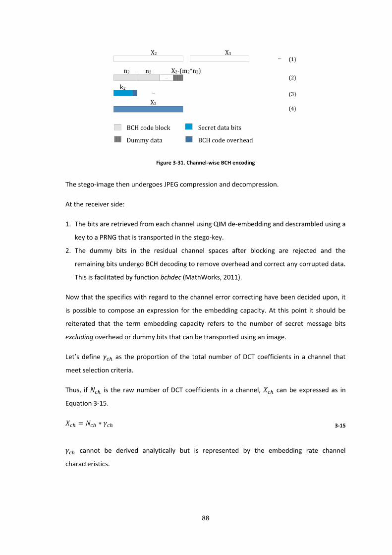
88
...
...
...
(1)
(2)
(3)
(4)
n2 n2 X2-(m2*n2)
X2
X2
k2
X3
Figure 3-31. Channel-wise BCH encoding
The stego-image then undergoes JPEG compression and decompression.
At the receiver side:
1. The bits are retrieved from each channel using QIM de-embedding and descrambled using a
key to a PRNG that is transported in the stego-key.
2. The dummy bits in the residual channel spaces after blocking are rejected and the
remaining bits undergo BCH decoding to remove overhead and correct any corrupted data.
This is facilitated by function bchdec (MathWorks, 2011).
Now that the specifics with regard to the channel error correcting have been decided upon, it
is possible to compose an expression for the embedding capacity. At this point it should be
reiterated that the term embedding capacity refers to the number of secret message bits
excluding overhead or dummy bits that can be transported using an image.
Let’s define as the proportion of the total number of DCT coefficients in a channel that
meet selection criteria.
Thus, if is the raw number of DCT coefficients in a channel, can be expressed as in
Equation 3-15.
3-15
cannot be derived analytically but is represented by the embedding rate channel
characteristics.
BCH code block
Dummy data BCH code overhead
Secret data bits
89
If is the BCH code block length used for a particular channel, the number of blocks in a
channel corresponds to the number of batches of that fit completely into . This is
shown in Equation 3-16.
(
* 3-16
where maps to the largest integer that does not exceed .
In each block there are secret message bits. Therefore, the number of secret message bits
(not overhead bits or dummy bits) in a channel is given in Equation 3-17.
(
*
3-17
The total number of secret message bits that can be accommodated in the image across all
channels, which we call embedding capacity, is given in Equation 3-18.
∑ (
*
3-18
3.6.2 Usable Channels & Per Channel Error Correction
So far, it has been confirmed that using channel characteristics and error code properties, data
handling parameters that give best embedding capacity for a channel can be derived. Now that
BCH coding has been decided upon and the embedding capacity can be derived, and
need to be considered more carefully and selected to maximise embedding capacity in each
channel.
First, a tolerance line needs to be selected to represent the error rate at each delta for which
error correcting will cater. Theoretically, if the values of delta and error correcting parameters
are derived according to 100% error rate tolerance lines then no errors should ever be
observed and error coding would not be required. In reality, it is possible that an outlier was
not characterised and rare errors may occur. Using a tolerance limit less than 100% would
certainly require error coding. Recall the 98% tolerance line for embedding rate was already
selected in Section 3.5.

90
The tolerance line for which error is corrected can be chosen at the discretion of the designer
and will depend on the amount of allowable error in a given channel. Before making the final
decision on what tolerance line to use, we can say that the 95% error rate tolerance line is a
reasonable boundary for the lowest tolerance percentage a moderate channel error correcting
scheme would cater for. Recall the 95% tolerance level for error rate represents the value of
error rate below which 95% of observable batch error rates have occurred.
Having defined a lower limit on what error rate tolerance limit to use, we can now consider
which channels are usable and which are not. We know that channels where the error rate is
consistently above 25% cannot be corrected for using BCH codes and correcting for high
error rates would go against the principle of attempting to increase embedding capacity since
a strong coding scheme and significant overhead would be required compromising embedding
capacity, bringing into doubt whether the channel should be used at all.
Not all channels have 95% tolerance lines indicating an error rate below 25%, and those that
do not are rejected for embedding according to the condition that only moderate error
correction is worthwhile. The channels that are deemed usable are highlighted in blue in
Figure 3-32.
The 12x12 matrix contains the channel numbers taken in zigzag order in MULTI. It is evident
now that 30 channels are usable in an E-block in conjunction with moderate error correction
contradicting the assumptions made in the literature previously that only the first 19 are
usable. Recall that the corresponding matrix for any E-block smaller than 12x12 can be
extracted by taking the required square from the top left hand corner of the matrix in Figure
3-32. All of the channels but one lie in the top left 8x8 segment of the E-blocks and so each E-
block will contribute one candidate coefficient towards these channels.
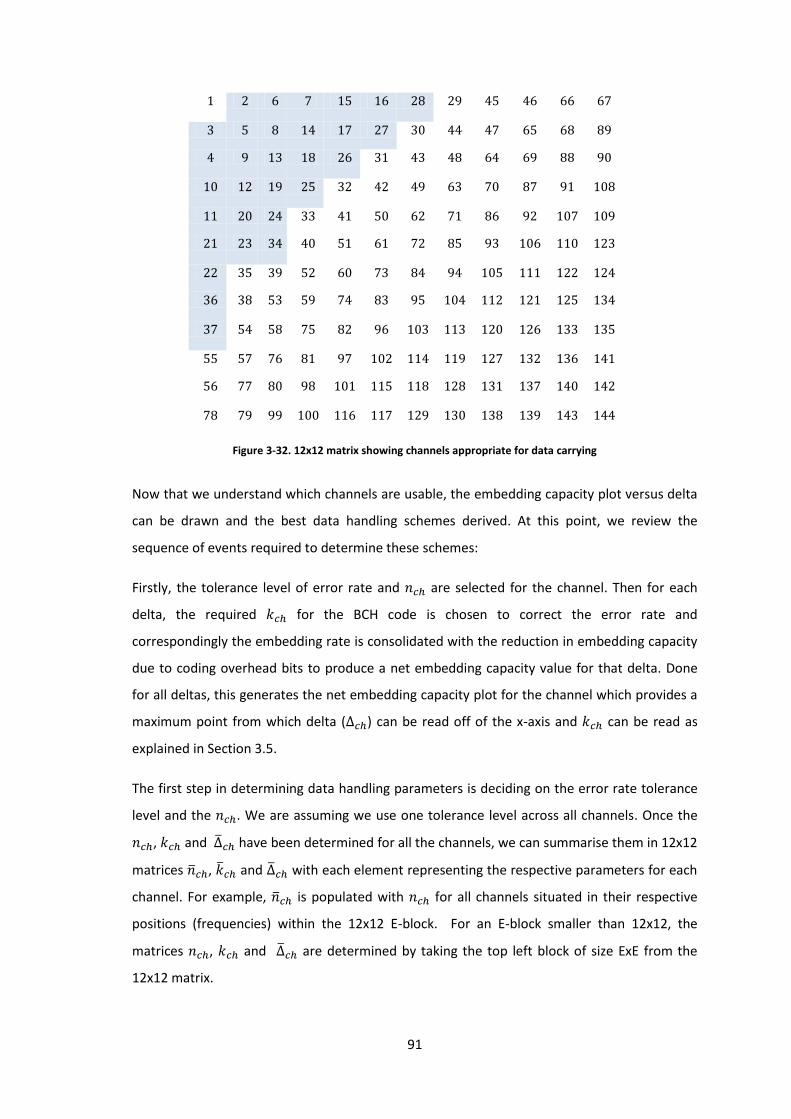
91
1 2 6 7 15 16 28 29 45 46 66 67
3 5 8 14 17 27 30 44 47 65 68 89
4 9 13 18 26 31 43 48 64 69 88 90
10 12 19 25 32 42 49 63 70 87 91 108
11 20 24 33 41 50 62 71 86 92 107 109
21 23 34 40 51 61 72 85 93 106 110 123
22 35 39 52 60 73 84 94 105 111 122 124
36 38 53 59 74 83 95 104 112 121 125 134
37 54 58 75 82 96 103 113 120 126 133 135
55 57 76 81 97 102 114 119 127 132 136 141
56 77 80 98 101 115 118 128 131 137 140 142
78 79 99 100 116 117 129 130 138 139 143 144
Figure 3-32. 12x12 matrix showing channels appropriate for data carrying
Now that we understand which channels are usable, the embedding capacity plot versus delta
can be drawn and the best data handling schemes derived. At this point, we review the
sequence of events required to determine these schemes:
Firstly, the tolerance level of error rate and are selected for the channel. Then for each
delta, the required for the BCH code is chosen to correct the error rate and
correspondingly the embedding rate is consolidated with the reduction in embedding capacity
due to coding overhead bits to produce a net embedding capacity value for that delta. Done
for all deltas, this generates the net embedding capacity plot for the channel which provides a
maximum point from which delta ( ) can be read off of the x-axis and can be read as
explained in Section 3.5.
The first step in determining data handling parameters is deciding on the error rate tolerance
level and the . We are assuming we use one tolerance level across all channels. Once the
, and have been determined for all the channels, we can summarise them in 12x12
matrices , and with each element representing the respective parameters for each
channel. For example, is populated with for all channels situated in their respective
positions (frequencies) within the 12x12 E-block. For an E-block smaller than 12x12, the
matrices , and are determined by taking the top left block of size ExE from the
12x12 matrix.
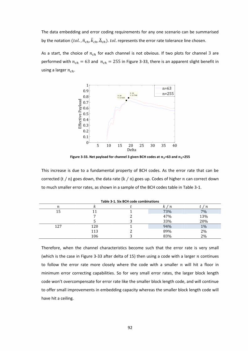
92
The data embedding and error coding requirements for any one scenario can be summarised
by the notation . represents the error rate tolerance line chosen.
As a start, the choice of for each channel is not obvious. If two plots for channel are
performed with and in Figure 3-33, there is an apparent slight benefit in
using a larger .
Figure 3-33. Net payload for channel 3 given BCH codes at =63 and =255
This increase is due to a fundamental property of BCH codes. As the error rate that can be
corrected ( ⁄ ) goes down, the data rate ( ⁄ ) goes up. Codes of higher can correct down
to much smaller error rates, as shown in a sample of the BCH codes table in Table 3-1.
Table 3-1. Six BCH code combinations
⁄ ⁄
Therefore, when the channel characteristics become such that the error rate is very small
(which is the case in Figure 3-33 after delta of 15) then using a code with a larger continues
to follow the error rate more closely where the code with a smaller will hit a floor in
minimum error correcting capabilities. So for very small error rates, the larger block length
code won’t overcompensate for error rate like the smaller block length code, and will continue
to offer small improvements in embedding capacity whereas the smaller block length code will
have hit a ceiling.
5 10 15 20 25 30 35 400
0.1
0.2
0.3
0.4
0.5
0.6
0.7
0.8
0.9
1
X: 18
Y: 0.7329
Eff
ecti
ve
Pay
load
Delta
X: 19
Y: 0.7749
n=63
n=255
93
Whether this minor advantage can compensate for the larger average ⁄ bits lost at the
end of the channel due to blocking will be seen shortly. Nevertheless, this result suggests that
where very small amounts of error correction are required, it is better to use schemes with
higher block lengths whereas at levels where both codes operate comfortably it is better to
use more efficient smaller block length codes. Also visible in Figure 3-33 is that gives
better embedding capacity for larger deltas whereas results in better embedding
capacity for smaller deltas.
With regard to choosing error rate tolerance limits, we defined a reasonable lower boundary
for moderate error correction as 95% in this section thus already accepting a significant
likelihood of error in each channel. The more error allowed in the system, the less the
embedding capacity is compromised and so we can see using the 100% tolerance line probably
won’t be a good choice.
At this point, we could ignore the fact that errors may be inevitable and delve further into the
question of selecting delta values and an error rate tolerance limit but the fact that some error
will probably need to be accepted in the system should be addressed first. With channel error
correcting alone, it is not possible to guarantee a low image error rate (i.e. the percentage of
stego-images that will provide erroneous data during QIM de-embedding) because we have no
control on when errors occur simultaneously in different channels.
In particular, this work is trying to keep error to an absolute minimum and since channel-wise
error correcting alone has limitations, this leads to the idea of implementing another layer of
error correction that can catch any errors that may occur in the channels and further minimise
error. This idea is discussed in the next section.
3.6.3 Image-Global Error Coding
It has already been discussed that a particular tolerance level of error rate under 100% would
probably need to be selected for the purposes of error correcting on a per channel basis. The
implication is then that with only the scheme described some degree of error is inevitable, and
we don’t have control over when channel errors occur simultaneously in an image. The
steganographer would require some guarantee that a certain high proportion of the images
he/she embeds into will provide error-free secret data to the recipient which cannot be
guaranteed with channel-wise error correcting alone.
Depending on the application, occasional errors in retrieved data may be acceptable. However,
this work is trying to cater for the more restricted case that error rate should be kept to a
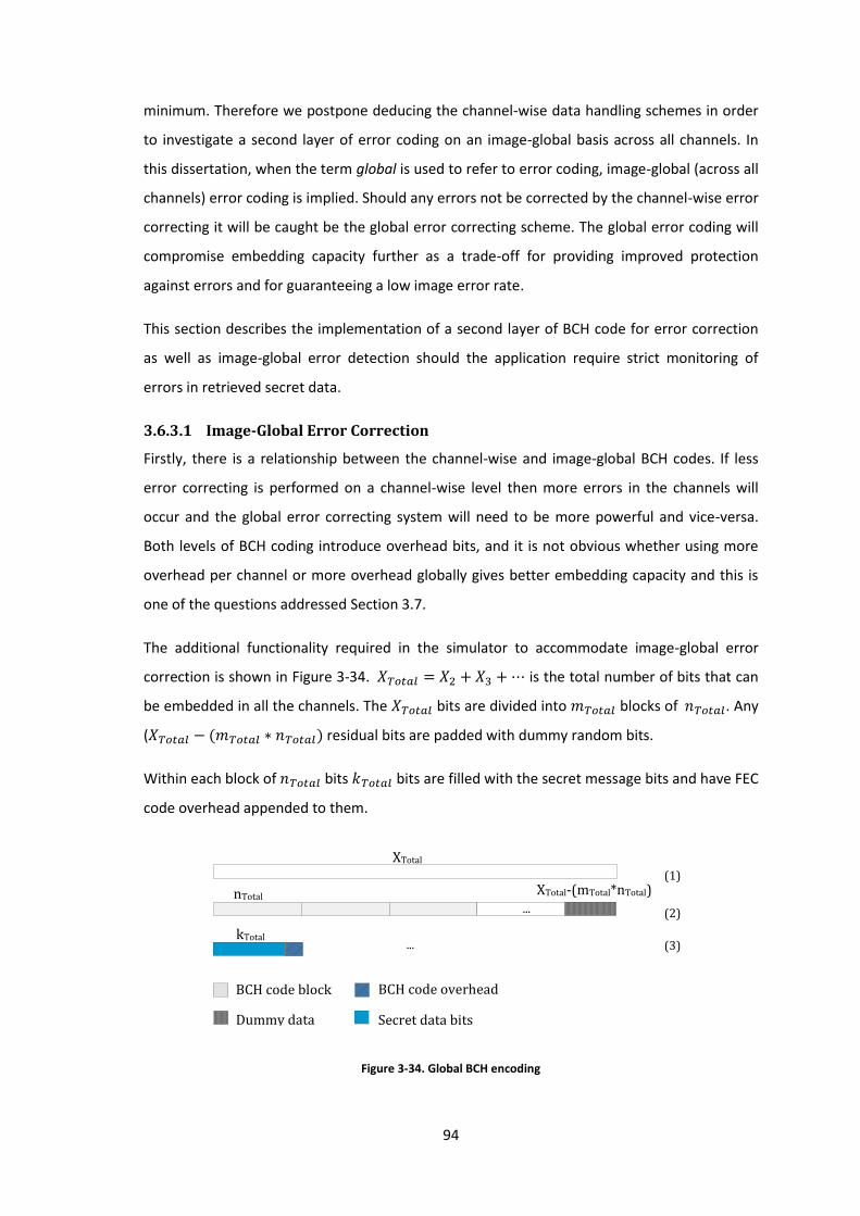
94
minimum. Therefore we postpone deducing the channel-wise data handling schemes in order
to investigate a second layer of error coding on an image-global basis across all channels. In
this dissertation, when the term global is used to refer to error coding, image-global (across all
channels) error coding is implied. Should any errors not be corrected by the channel-wise error
correcting it will be caught be the global error correcting scheme. The global error coding will
compromise embedding capacity further as a trade-off for providing improved protection
against errors and for guaranteeing a low image error rate.
This section describes the implementation of a second layer of BCH code for error correction
as well as image-global error detection should the application require strict monitoring of
errors in retrieved secret data.
3.6.3.1 Image-Global Error Correction
Firstly, there is a relationship between the channel-wise and image-global BCH codes. If less
error correcting is performed on a channel-wise level then more errors in the channels will
occur and the global error correcting system will need to be more powerful and vice-versa.
Both levels of BCH coding introduce overhead bits, and it is not obvious whether using more
overhead per channel or more overhead globally gives better embedding capacity and this is
one of the questions addressed Section 3.7.
The additional functionality required in the simulator to accommodate image-global error
correction is shown in Figure 3-34. is the total number of bits that can
be embedded in all the channels. The bits are divided into blocks of . Any
( residual bits are padded with dummy random bits.
Within each block of bits bits are filled with the secret message bits and have FEC
code overhead appended to them.
...
XTotal
XTotal-(mTotal*nTotal)nTotal
kTotal...
(1)
(2)
(3)
Figure 3-34. Global BCH encoding
Dummy data
BCH code block BCH code overhead
Secret data bits
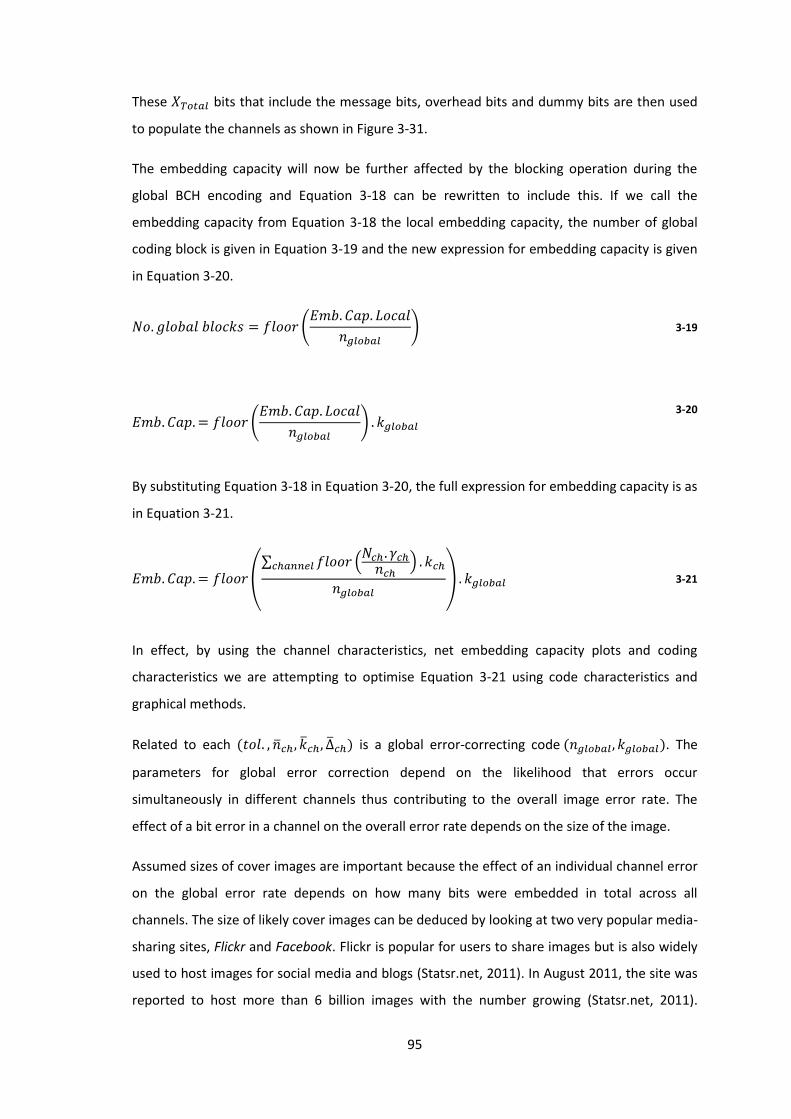
95
These bits that include the message bits, overhead bits and dummy bits are then used
to populate the channels as shown in Figure 3-31.
The embedding capacity will now be further affected by the blocking operation during the
global BCH encoding and Equation 3-18 can be rewritten to include this. If we call the
embedding capacity from Equation 3-18 the local embedding capacity, the number of global
coding block is given in Equation 3-19 and the new expression for embedding capacity is given
in Equation 3-20.
(
) 3-19
(
)
3-20
By substituting Equation 3-18 in Equation 3-20, the full expression for embedding capacity is as
in Equation 3-21.
(∑ (
)
) 3-21
In effect, by using the channel characteristics, net embedding capacity plots and coding
characteristics we are attempting to optimise Equation 3-21 using code characteristics and
graphical methods.
Related to each is a global error-correcting code . The
parameters for global error correction depend on the likelihood that errors occur
simultaneously in different channels thus contributing to the overall image error rate. The
effect of a bit error in a channel on the overall error rate depends on the size of the image.
Assumed sizes of cover images are important because the effect of an individual channel error
on the global error rate depends on how many bits were embedded in total across all
channels. The size of likely cover images can be deduced by looking at two very popular media-
sharing sites, Flickr and Facebook. Flickr is popular for users to share images but is also widely
used to host images for social media and blogs (Statsr.net, 2011). In August 2011, the site was
reported to host more than 6 billion images with the number growing (Statsr.net, 2011).
96
Facebook has already been introduced in Chapter 1. Since the beginning of 2011, Facebook has
ranked as the most used social networking service worldwide (Facebook, 2011). Given these
statistics, the size of images used on these websites provides a good indication for general
trends in digital image sharing.
On Facebook, a standard image may be up to 960x960 (Facebook, 2011), while on Flickr a
small image is categorised as 180x240 and a medium image 375x500 (Statsr.net, 2011). The
trend is that the size and quality of the images hosted by these websites is gradually
increasing. Therefore, in this dissertation, the categories of image sizes are taken as:
Small – around 180x240, these images provide roughly 300 E-blocks using MULTI
Medium - around 375x600, these images provide roughly 1500 E-blocks using MULTI
Large – any image 50% or more greater in number of pixels than medium-sized images
Given the infinite variability in image content, it is impossible to analytically determine
dependencies between channels but an estimate can be made using a random set of 200
images not including those used to deduce the channel characteristics. By monitoring the
global error in each of these images, can be deduced for each possibility of
according to the maximum observed error.
The acceptable image error rate depends on the nature of the data being transmitted and the
patience of the steganographer! For example, some distortion in a video recording will not
have the same effect as a shifted decimal place on a bank balance. If the steganographer
wishes to check that an image is in error before transmission, he/she can JPEG compress and
decompress the stego-image as if it were going through the channel and retrieve the data.
Comparing it to the intended secret message would reveal an error and if erroneous the
process of embedding and checking could continue until the secret message is found to be
transmitted perfectly. However, a steganographer may not like to do this or may become
frustrated if many images are in error.
We now deal with setting an image-global error rate (which from now on will be referred to as
a global error rate) at a particular level and by using tests deduce global error coding
parameters required to meet this.
In this dissertation, an arbitrary though reasonable requirement that less than 1% of observed
images have error is insisted upon. Although previously it was said that related to each
is a global error-correcting code , for the purposes of
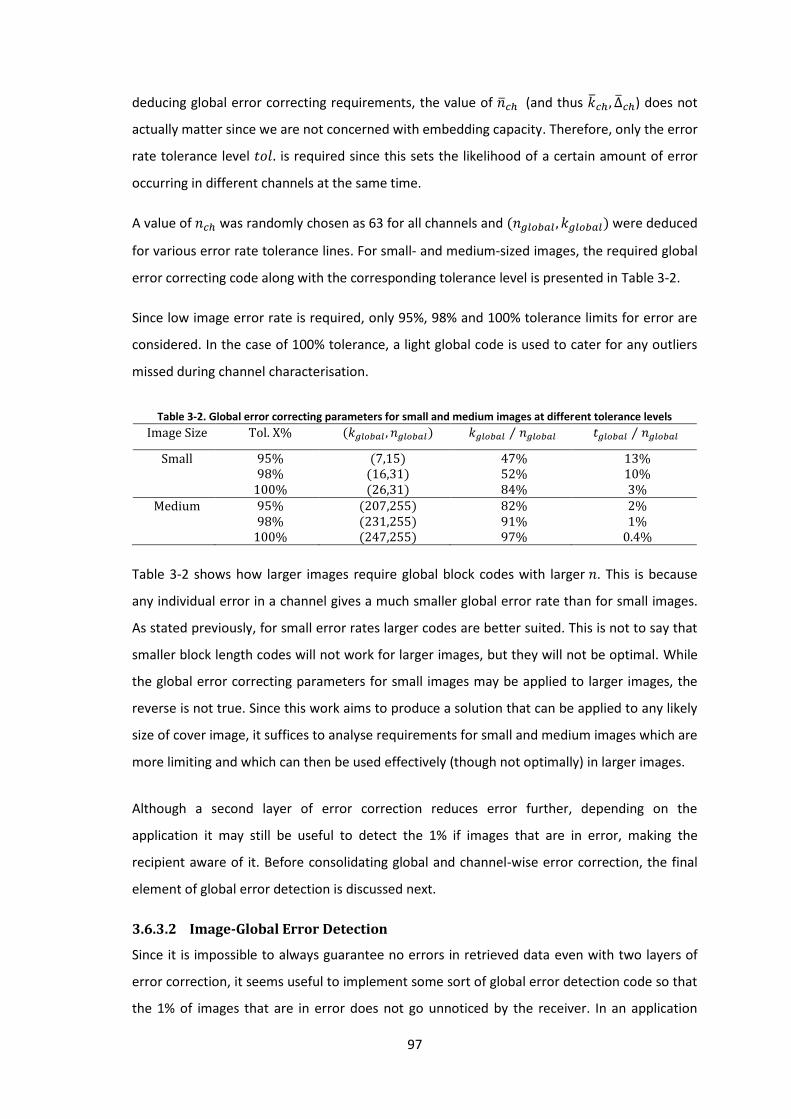
97
deducing global error correcting requirements, the value of (and thus ) does not
actually matter since we are not concerned with embedding capacity. Therefore, only the error
rate tolerance level is required since this sets the likelihood of a certain amount of error
occurring in different channels at the same time.
A value of was randomly chosen as 63 for all channels and were deduced
for various error rate tolerance lines. For small- and medium-sized images, the required global
error correcting code along with the corresponding tolerance level is presented in Table 3-2.
Since low image error rate is required, only 95%, 98% and 100% tolerance limits for error are
considered. In the case of 100% tolerance, a light global code is used to cater for any outliers
missed during channel characterisation.
Table 3-2. Global error correcting parameters for small and medium images at different tolerance levels
Image Size Tol. X% ⁄ ⁄
Small
Medium
Table 3-2 shows how larger images require global block codes with larger . This is because
any individual error in a channel gives a much smaller global error rate than for small images.
As stated previously, for small error rates larger codes are better suited. This is not to say that
smaller block length codes will not work for larger images, but they will not be optimal. While
the global error correcting parameters for small images may be applied to larger images, the
reverse is not true. Since this work aims to produce a solution that can be applied to any likely
size of cover image, it suffices to analyse requirements for small and medium images which are
more limiting and which can then be used effectively (though not optimally) in larger images.
Although a second layer of error correction reduces error further, depending on the
application it may still be useful to detect the 1% if images that are in error, making the
recipient aware of it. Before consolidating global and channel-wise error correction, the final
element of global error detection is discussed next.
3.6.3.2 Image-Global Error Detection
Since it is impossible to always guarantee no errors in retrieved data even with two layers of
error correction, it seems useful to implement some sort of global error detection code so that
the 1% of images that are in error does not go unnoticed by the receiver. In an application

98
where perfect data recovery is important, on the rare occasion that an error is detected the
receiver can request the sender to retransmit the secret message using a different cover
image. Again, there is no natural mechanism for feedback but requests for retransmission over
some sort of a feedback channel 1% of the time are not substantially suspicious. This section
describes implementation of global error detection for this purpose.
The simplest form of error detection is the use of the parity bit. The bit is designated to
represent whether there are an odd or even number of 1’s in a given bit stream. If the values
of the parity bit and data stream are not in agreement, an error has occurred. The parity bit is
a special case of what are known as cycle redundancy check (CRC) codes (Kuo, Lee, & Tian,
2006). A CRC code is based on polynomial arithmetic. It is calculated by treating the input data
message as a polynomial, e.g. the message 11001001 would be treated as .
This polynomial is then divided by a fixed polynomial agreed upon by the sender and receiver.
The resultant remainder is appended to the input data and the receiver can then detect errors.
The fixed polynomial is called a generator polynomial related to the CRC code. There are
many possible generator polynomials that can be chosen and selecting the correct one is an
important part of successfully implementing error detection. The polynomial depends on the
amount of data to be protected, the required error protection and performance.
Some common characteristics of performance include:
(a) If contains two or more terms then all single-bit errors are detected.
(b) If x+1 is a factor (i.e. if has an even number of non-zero coefficients) of then all
odd number of erroneous bits are detected.
(c) A CRC checksum of order r can detect burst errors of length less than or equal to .
Table 3-3 shows the generator polynomials according to some common standards
(Hackersdelight.org, 2009).
Table 3-3. Generator polynomials of some common standards in CRC codes
Code Generator Polynomial g(x)
CRC-8
CRC-12
CRC-16
To cater for small errors, a light CRC-8 code is implemented decreasing payload by only 8 bits.
The CRC code is implemented using in-built functions and the corresponding generator
polynomial (MathWorks, 2011).
99
3.7 Selecting Error Coding Parameters for YASS2/MULTI2
Now that channel-wise and global error correcting and global error detection have been
discussed, all of the elements of error coding have been covered and we now return to
determining the the final data handling schemes.
Up until now the specifics regarding local error correcting have been discussed and, using net
embedding capacity plots for each block size of BCH codes, the data handling procedures
that give best embedding capacity for a channel have been derived. In the process we have
discovered that a second layer of global image error correction across channels in an image is
required to keep the image error rate sufficiently low and the global error correcting
parameters have been deduced for different error rate tolerance lines from the channel
characteristics. In the case that an image does provide erroneous data at the receiver, a light
CRC error detection code is implemented should the application require strict monitoring of
errors.
All together the local and global data embedding and error correcting parameters can be
described as . So far the dissertation has addressed how to
determine best embedding capacity points for each channel for and . Associated with
each ( ) is a global ( ) which was determined in Table 3-2 using
tests for each error rate tolerance level.
Now that these possibilities have been deduced, we are required to determine which
possibility gives best embedding capacity generally across stego-images.
First, in order to determine which error rate tolerance line to use, a random set of 200 images
was selected from the database. Each scenario of global error correction in Table 3-2 was
implemented in turn for both image sizes with set to be uniform across channels and for
the situations that 31, 63, 127, 255. For each , using the 98% error rate tolerance
case resulted in the best embedding capacity for 60-70% of the images for all sizes and so was
chosen.
Now that the 98% error rate tolerance limit has been chosen to give the best trade-off
between local and global error correction, needs to be chosen. In the 98% case, the
statistics gathered for small and medium images is shown in Table 3-4 and Table 3-5 when
using one for all channels.
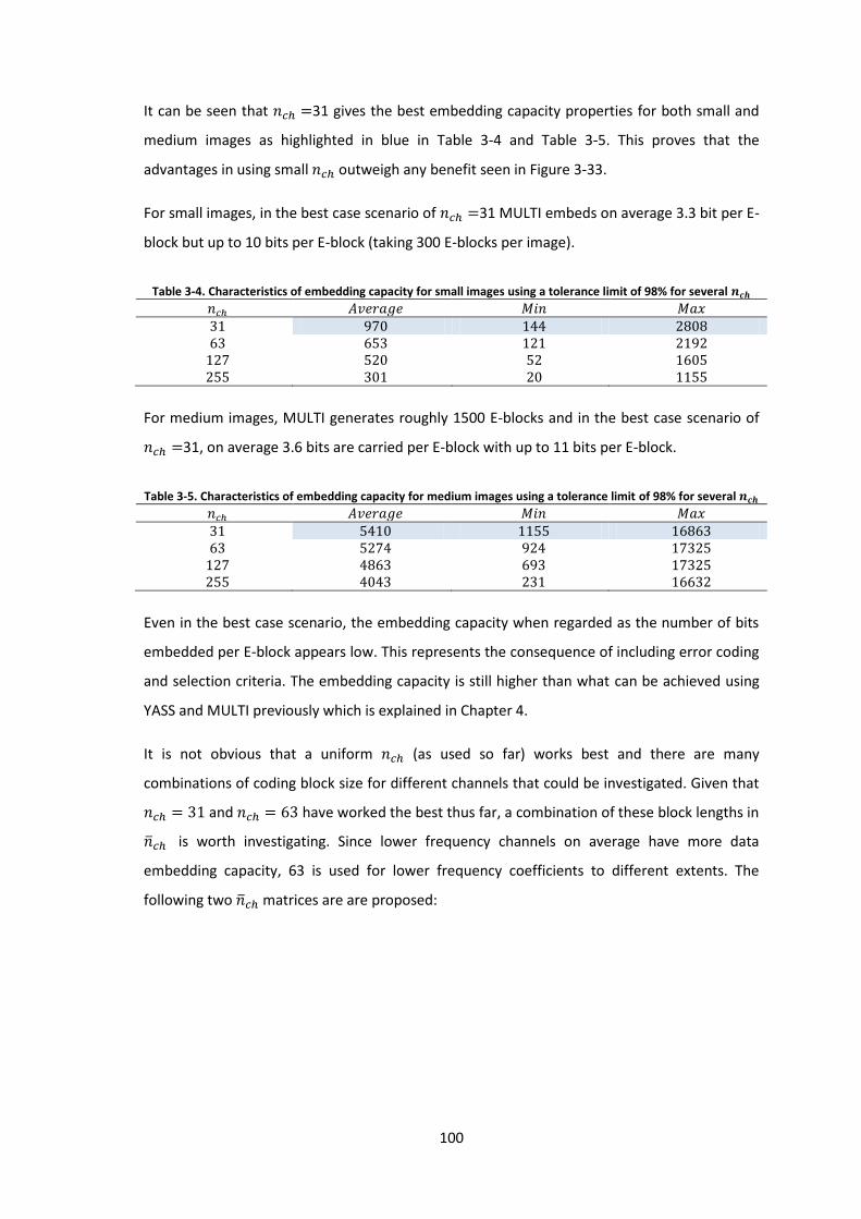
100
It can be seen that 31 gives the best embedding capacity properties for both small and
medium images as highlighted in blue in Table 3-4 and Table 3-5. This proves that the
advantages in using small outweigh any benefit seen in Figure 3-33.
For small images, in the best case scenario of 31 MULTI embeds on average 3.3 bit per E-
block but up to 10 bits per E-block (taking 300 E-blocks per image).
Table 3-4. Characteristics of embedding capacity for small images using a tolerance limit of 98% for several
For medium images, MULTI generates roughly 1500 E-blocks and in the best case scenario of
31, on average 3.6 bits are carried per E-block with up to 11 bits per E-block.
Table 3-5. Characteristics of embedding capacity for medium images using a tolerance limit of 98% for several
Even in the best case scenario, the embedding capacity when regarded as the number of bits
embedded per E-block appears low. This represents the consequence of including error coding
and selection criteria. The embedding capacity is still higher than what can be achieved using
YASS and MULTI previously which is explained in Chapter 4.
It is not obvious that a uniform (as used so far) works best and there are many
combinations of coding block size for different channels that could be investigated. Given that
and have worked the best thus far, a combination of these block lengths in
is worth investigating. Since lower frequency channels on average have more data
embedding capacity, 63 is used for lower frequency coefficients to different extents. The
following two matrices are are proposed:
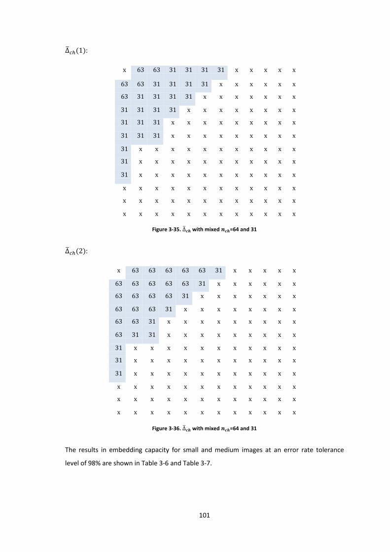
101
:
x 63 63 31 31 31 31 x x x x x
63 63 31 31 31 31 x x x x x x
63 31 31 31 31 x x x x x x x
31 31 31 31 x x x x x x x x
31 31 31 x x x x x x x x x
31 31 31 x x x x x x x x x
31 x x x x x x x x x x x
31 x x x x x x x x x x x
31 x x x x x x x x x x x
x x x x x x x x x x x x
x x x x x x x x x x x x
x x x x x x x x x x x x
Figure 3-35. with mixed =64 and 31
:
x 63 63 63 63 63 31 x x x x x
63 63 63 63 63 31 x x x x x x
63 63 63 63 31 x x x x x x x
63 63 63 31 x x x x x x x x
63 63 31 x x x x x x x x x
63 31 31 x x x x x x x x x
31 x x x x x x x x x x x
31 x x x x x x x x x x x
31 x x x x x x x x x x x
x x x x x x x x x x x x
x x x x x x x x x x x x
x x x x x x x x x x x x
Figure 3-36. with mixed =64 and 31
The results in embedding capacity for small and medium images at an error rate tolerance
level of 98% are shown in Table 3-6 and Table 3-7.
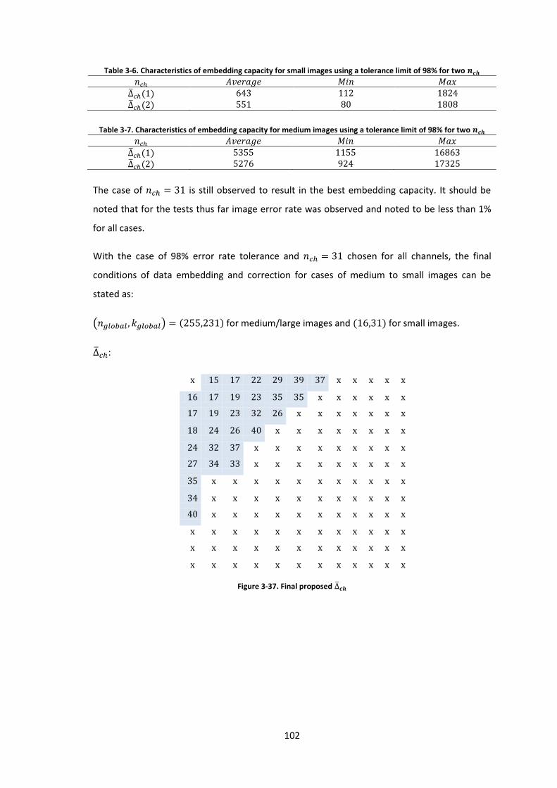
102
Table 3-6. Characteristics of embedding capacity for small images using a tolerance limit of 98% for two
Table 3-7. Characteristics of embedding capacity for medium images using a tolerance limit of 98% for two
The case of is still observed to result in the best embedding capacity. It should be
noted that for the tests thus far image error rate was observed and noted to be less than 1%
for all cases.
With the case of 98% error rate tolerance and chosen for all channels, the final
conditions of data embedding and correction for cases of medium to small images can be
stated as:
( ) for medium/large images and for small images.
:
x 15 17 22 29 39 37 x x x x x
16 17 19 23 35 35 x x x x x x
17 19 23 32 26 x x x x x x x
18 24 26 40 x x x x x x x x
24 32 37 x x x x x x x x x
27 34 33 x x x x x x x x x
35 x x x x x x x x x x x
34 x x x x x x x x x x x
40 x x x x x x x x x x x
x x x x x x x x x x x x
x x x x x x x x x x x x
x x x x x x x x x x x x
Figure 3-37. Final proposed
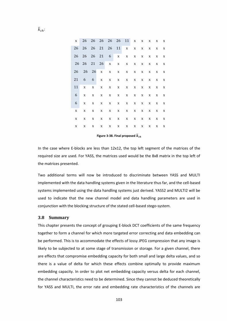
103
:
x 26 26 26 26 26 11 x x x x x
26 26 26 21 26 11 x x x x x x
26 26 26 21 6 x x x x x x x
26 21 26 x x x x x x x x
26 x x x x x x x x x
21 6 6 x x x x x x x x x
11 x x x x x x x x x x x
6 x x x x x x x x x x x
6 x x x x x x x x x x x
x x x x x x x x x x x x
x x x x x x x x x x x x
x x x x x x x x x x x x
Figure 3-38. Final proposed
In the case where E-blocks are less than 12x12, the top left segment of the matrices of the
required size are used. For YASS, the matrices used would be the 8x8 matrix in the top left of
the matrices presented.
Two additional terms will now be introduced to discriminate between YASS and MULTI
implemented with the data handling systems given in the literature thus far, and the cell-based
systems implemented using the data handling systems just derived. YASS2 and MULTI2 will be
used to indicate that the new channel model and data handling parameters are used in
conjunction with the blocking structure of the stated cell-based stego-system.
3.8 Summary
This chapter presents the concept of grouping E-block DCT coefficients of the same frequency
together to form a channel for which more targeted error correcting and data embedding can
be performed. This is to accommodate the effects of lossy JPEG compression that any image is
likely to be subjected to at some stage of transmission or storage. For a given channel, there
are effects that compromise embedding capacity for both small and large delta values, and so
there is a value of delta for which these effects combine optimally to provide maximum
embedding capacity. In order to plot net embedding capacity versus delta for each channel,
the channel characteristics need to be determined. Since they cannot be deduced theoretically
for YASS and MULTI, the error rate and embedding rate characteristics of the channels are
104
deduced over a sufficiently varying image database until they converge. The resultant channel
characteristic plots are scatter plots from which tolerance lines can be derived that link error
and embedding rate values at a particular delta below which a certain percentage of rate
measurements have occurred.
Specifically, BCH codes are appropriate for this application and allow moderate error
correction with relatively low overhead. By consolidating the properties of BCH codes with the
channel characteristics of 30 usable channels, data embedding and error correcting
parameters were found that maximise embedding capacity. Corresponding to a particular set
of channel embedding and correcting schemes is an image-global error correcting scheme that
aims to correct any residual errors and finally, the implementation of a CRC error detection
code to catch any errors that may creep through. The global error correction was set so that
1% of images may show error. It was finally shown that from a reasonable set of possibilities,
using an error rate tolerance line of 98% with BCH code block size being 31 for all channels
should give good embedding capacity across all stego-image sizes. The derived data handling
systems used in conjunction with block structure of existing cell-based systems are indicated
by 2, as in for example YASS2.
105
Chapter 4. Analysis of the Scheme
Cell-based systems are relevant given their good security properties and the fact that they
cater for the likely eventuality that a stego-image will undergo JPEG compression at some
stage in its transmission and storage. In Chapter 3, the idea was presented of improving data
embedding and error correcting schemes in cell-based systems using a channel model that
connects E-block DCT coefficients of the same frequency together so that one image contains
up to 144 channels depending on the cell-based system used. Following on from this, channel
characteristics were determined which, combined with error coding requirements and general
limits on stego-image size, lead to the proposal of channel-wise and image-global data
handling parameters that give good embedding capacity properties.
This chapter tests these parameters further by placing them back into context and testing
YASS2 and MULTI2 for security. The self-imposed boundary on image error rate of 1% is also
further verified and some final comments regarding embedding capacity improvements are
made.
4.1 Steganalysis
The data embedding and error coding parameters have been determined without specific
mention of testing security against blind steganalysers. This is because it was assumed that the
random nature of embedding would ensure security even if delta values were altered. In this
section, the performance of YASS2 and MULTI2 are tested against a prominent steganalyser to
analyse this assumption and to check that good security properties have been maintained.
4.1.1 Detection Rate
With regard to resistance of a stego-system against steganalysis, the result that determines
security of a particular system is detection rate , which represents the likelihood of a
steganalyser correctly identifying a stego-image. More mathematically, it can be represented
as shown in Equation 4-1.
4-1
where is the likelihood of the steganalyser making a mistake in classifying a given image
as innocent or corrupt. A steganalyser is in error if it falsely categorises an innocent cover-
image as corrupt, or a corrupt stego-image as innocent. Let be the event that an innocent
image is analysed and be the event that a corrupt stego-image is analysed. Let be the
event that the steganalyser detects an innocent image and be the event that the
106
steganalyser detects a data carrying stego-image. Then can be written as in Equation
4-2.
4-2
Define and as false negative and false positive rates and respectively,
then Equation 4-2 may be written as Equation 4-3.
4-3
Assuming that the same number of innocent and corrupt images are presented to the
steganalyser, ⁄ . Therefore, Equation 4-1 can be rewritten as Equation 4-4.
⁄
⁄ 4-4
Let’s assume the most primitive of steganalysers where it classifies all images as always either
innocent or corrupt. Given an equal likelihood of either type of image ⁄
and ⁄ .
Therefore, we consider a stego-system secure if a blind steganalyser has a detection rate of 0.5
implying it is taking a guess with each classification, with a detection rate of under 0.6
considered to be adequately secure (Dawoud, 2010).
4.1.2 Resistance against PF-274
Among blind steganalysers that exist in the literature, (Pevny & Fridrich, 2006) and (Pevny &
Fridrich, 2007) are considered the most effective and are used to test security in the cell-based
system literature. In this thesis, the scheme will be referred to as PF-274.
The functionality of a blind steganalyser has been referred to throughout this dissertation.
Blind steganalysers do not assume any particular stego-system, but aim to determine features
of an image that tend to distinguish corrupt stego-images from innocent cover images and
which they can use in conjunction with a large number of images to train a classifier. In
particular, finding the correct features that vary with embedding but not with natural variation
between image content is the most challenging element of implementation. The feature set is
usually large and is derived from many statistical characteristics of an image.
107
(Pevny & Fridrich, 2006) describe that traditionally classifiers have used two types of features:
DCT features and Markov features. DCT features are a set of parameters derived from the
distribution of DCT coefficients in both the RGB and YCbCr colour spaces, statistics regarding
change in DCT coefficients in different directions and the inter-block dependencies between
DCT coefficients. The Markov feature set produces a model of the absolute difference of
neighbouring DCT coefficients. As the name implies, it produces a Markov model which is
effectively a statistical process where each future state is only conditionally dependent on the
directly-preceding state (Weisstein, 2011). The specifics of the mathematics are beyond the
scope of this dissertation and may be found in the quoted papers, but the gist of (Pevny &
Fridrich, 2006) is the idea that Markov features capture intra-block dependency among DCT
coefficients of similar spatial frequencies within the same 8x8 block whereas DCT features
model inter-block dependencies. In this way the two features used together complement each
other and, as the paper shows, they enhance performance when used together with the
disadvantage that more images need to be used for training given a larger training feature set.
Contact was made with the authors of (Pevny & Fridrich, 2006) and (Pevny & Fridrich, 2007),
and code was received that extracted 274 features from images. However, there was no code
to train a classifier with these features. Therefore, modules were written in Matlab that took
images from the image database (Schaefer & Stich, 2004) and which, in conjunction with the
received code, was used to extract the 274-element vector from each image and to insert it
into a matrix with as many columns as images. The features were then used to train an
analyser using 2000 images – 1000 innocent and 1000 corrupt images, giving two [274 1000]
matrices (with each row corresponding to a particular extracted feature). The corrupt images
were generated using the cell-based systems with embedding at full capacity. The images were
medium-size images, 375x500.
Using these matrices, the Neural Network Toolbox (MathWorks, 2011) was used to train the
neural network with a mixture of the innocent and corrupt features. Neural networks operate
in 3 steps:
1. By training themselves through recognising and grouping patterns or trends in a given
feature set.
2. The resultant neural network then undergoes validation where the generalisation of the
network is measured and where training is stopped to prevent the neural network from
becoming too fitted to the training images.
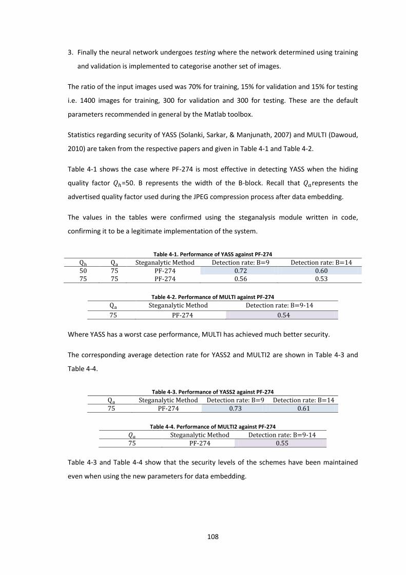
108
3. Finally the neural network undergoes testing where the network determined using training
and validation is implemented to categorise another set of images.
The ratio of the input images used was 70% for training, 15% for validation and 15% for testing
i.e. 1400 images for training, 300 for validation and 300 for testing. These are the default
parameters recommended in general by the Matlab toolbox.
Statistics regarding security of YASS (Solanki, Sarkar, & Manjunath, 2007) and MULTI (Dawoud,
2010) are taken from the respective papers and given in Table 4-1 and Table 4-2.
Table 4-1 shows the case where PF-274 is most effective in detecting YASS when the hiding
quality factor =50. B represents the width of the B-block. Recall that represents the
advertised quality factor used during the JPEG compression process after data embedding.
The values in the tables were confirmed using the steganalysis module written in code,
confirming it to be a legitimate implementation of the system.
Table 4-1. Performance of YASS against PF-274
Steganalytic Method Detection rate: B=9 Detection rate: B=14 PF-274 PF-274
Table 4-2. Performance of MULTI against PF-274
Steganalytic Method Detection rate: B=9-14
PF-274
Where YASS has a worst case performance, MULTI has achieved much better security.
The corresponding average detection rate for YASS2 and MULTI2 are shown in Table 4-3 and
Table 4-4.
Table 4-3. Performance of YASS2 against PF-274
Steganalytic Method Detection rate: B=9 Detection rate: B=14 PF-274 0.73
Table 4-4. Performance of MULTI2 against PF-274
Steganalytic Method Detection rate: B=9-14 PF-274
Table 4-3 and Table 4-4 show that the security levels of the schemes have been maintained
even when using the new parameters for data embedding.
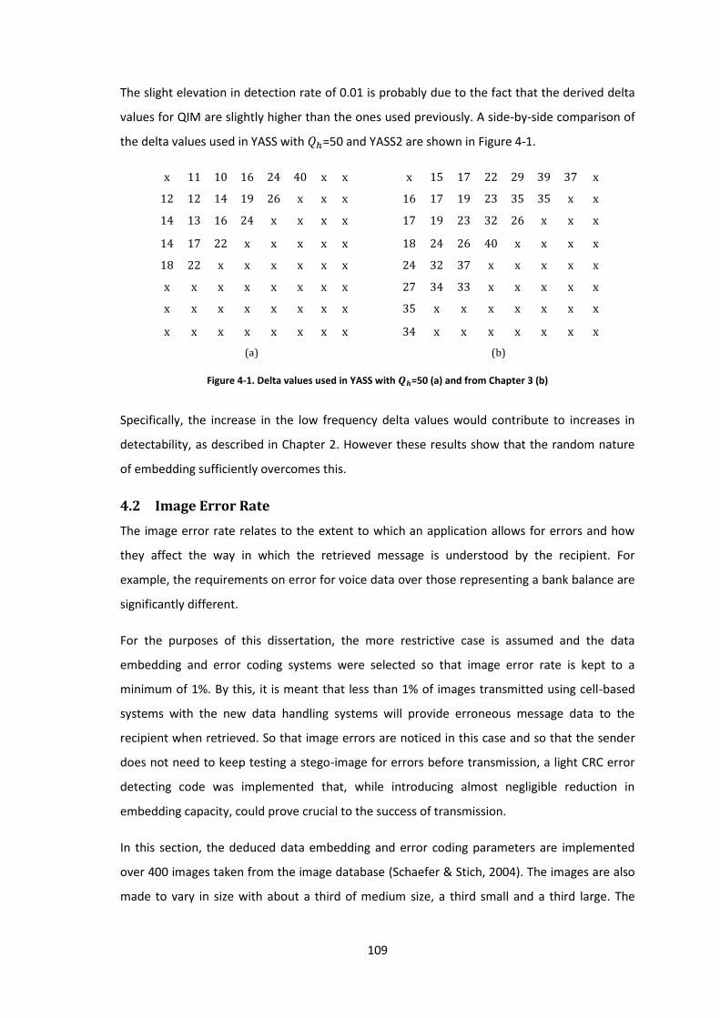
109
The slight elevation in detection rate of 0.01 is probably due to the fact that the derived delta
values for QIM are slightly higher than the ones used previously. A side-by-side comparison of
the delta values used in YASS with =50 and YASS2 are shown in Figure 4-1.
x 11 10 16 24 40 x x x 15 17 22 29 39 37 x
12 12 14 19 26 x x x 16 17 19 23 35 35 x x
14 13 16 24 x x x x 17 19 23 32 26 x x x
14 17 22 x x x x x 18 24 26 40 x x x x
18 22 x x x x x x 24 32 37 x x x x x
x x x x x x x x 27 34 33 x x x x x
x x x x x x x x 35 x x x x x x x
x x x x x x x x 34 x x x x x x x
(a) (b)
Figure 4-1. Delta values used in YASS with =50 (a) and from Chapter 3 (b)
Specifically, the increase in the low frequency delta values would contribute to increases in
detectability, as described in Chapter 2. However these results show that the random nature
of embedding sufficiently overcomes this.
4.2 Image Error Rate
The image error rate relates to the extent to which an application allows for errors and how
they affect the way in which the retrieved message is understood by the recipient. For
example, the requirements on error for voice data over those representing a bank balance are
significantly different.
For the purposes of this dissertation, the more restrictive case is assumed and the data
embedding and error coding systems were selected so that image error rate is kept to a
minimum of 1%. By this, it is meant that less than 1% of images transmitted using cell-based
systems with the new data handling systems will provide erroneous message data to the
recipient when retrieved. So that image errors are noticed in this case and so that the sender
does not need to keep testing a stego-image for errors before transmission, a light CRC error
detecting code was implemented that, while introducing almost negligible reduction in
embedding capacity, could prove crucial to the success of transmission.
In this section, the deduced data embedding and error coding parameters are implemented
over 400 images taken from the image database (Schaefer & Stich, 2004). The images are also
made to vary in size with about a third of medium size, a third small and a third large. The
110
purpose of these experiments was to verify that image error rate was below the 1% target set
and that CRC error detection code does detect all errors.
The steps for determining image error rate were:
1. The 400 images were embedded into using all available capacity in all of the channels using
the MULTI blocking systems and determined from
Chapter 3. All of the error correcting and detecting mechanisms were in place.
2. The input messages to the images were stored separately.
3. The images underwent JPEG compression and decompression using an advertised quality
factor of 75.
4. The data was then retrieved from the image using the data de-embedding and error
correcting systems. CRC error detection was also performed on the images, which showed
which images were detected to be in error.
5. The retrieved messages from the images were compared to the original input messages to
identify which images were actually in error.
The detected and actual errors were then compared. The CRC code detected all errors and out
of 400 images only 3 were found to be in error, with 0.2% of bits in error average across the 3
images. Two of the images in error were medium-sized and one was large-sized. This confirms
that an image error rate of 1% has been maintained and that the CRC code has operated
correctly in detecting cases of error.
4.3 Embedding Capacity
In Chapter 3, the process of identifying data embedding and error coding systems could be
divided into two parts. The first was the determination of different possibilities of
that met security, error rate and embedding capacity
requirements which stemmed from the new definition of a channel. The second part involved
selecting a case from the possibilities such that the requirements would be met across all
image sizes and contents. Since the derivation of the parameters themselves demonstrated
that good properties can be produced, these tests will not be repeated here. Rather, this
section concentrates on comparing relative performance between YASS2/MULTI2 and
YASS/MULTI and on stating embedding capacity as a proportion of image size.
4.3.1.1 Comparison to YASS and MULTI
It should be highlighted again that the focus of existing cell-based systems literature has not
been to address particulars regarding appropriateness of data embedding and error coding
111
parameters. Therefore, a direct comparison between embedding capacities achieved using
YASS or MULTI data embedding parameters and those using YASS2 or MULTI2 would not be
particularly fair or relevant as the original papers were not attempting to maximise capacity.
However, making a comparison can serve 2 purposes:
The comparison is required to confirm that in fact some improvement was made over the
original system, and that versus original rough propositions on data handling, a
steganographer using YASS2 or MULTI2 would indeed be able to transmit more data per
image than previously.
One of the goals of this research was to determine the extent to which channels more
volatile than the first 19 could be used in combination with error coding to produce a
substantial increase in embedding capacity. By comparing the embedding capacities
achieved, an overview of the extent to which the use of these channels benefits embedding
capacity can be found.
The comparisons were made by taking two identical images, and by determining the amount
of space for data in YASS using only the first 19 coefficients, with selection criteria using the
delta values given the JPEG quantisation matrix dictated by a hiding factor and using a RA
code with a factor of 10. Using a code rate of is a very optimistic estimate because
(Solanki, Sarkar, & Manjunath, 2007) recorded using a repeat rate of between 10 and 40,
meaning the best case scenario has been taken here.
YASS2 was then implemented and the embedding capacity was measured. It is not informative
to perform the comparison for MULTI too because YASS and MULTI only really differ in E-block
sizes and since the usable channels (apart from one) are contained in the first top left 8x8 cell
in each E-block there is no real benefit in performing the comparison for MULTI again. For each
image, the ratio of the two embedding capacity values were taken, with the embedding
capacity using YASS2 as the numerator. For these tests, 100 small and medium –sized images
were used.
Since (Solanki, Sarkar, & Manjunath, 2007) performed tests using 50 and 75, a
comparison to YASS is made at both of the hiding factors and a histogram of gain in embedding
capacity is shown in Figure 4-2.
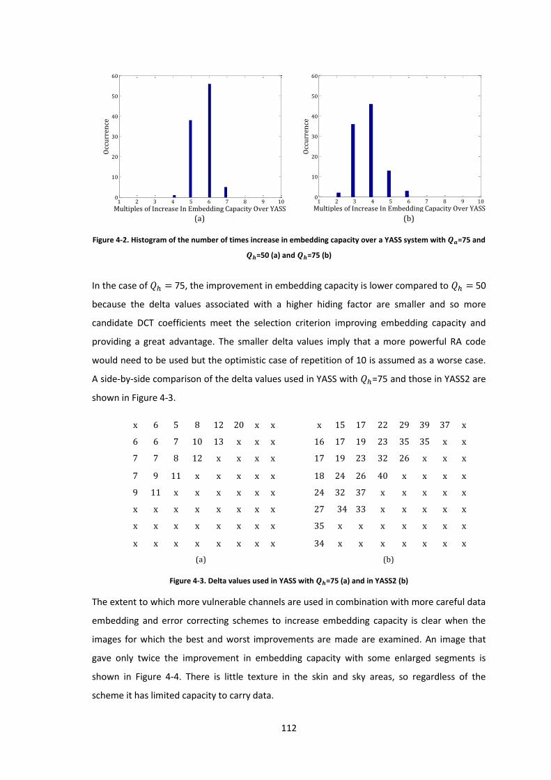
112
Figure 4-2. Histogram of the number of times increase in embedding capacity over a YASS system with =75 and
=50 (a) and =75 (b)
In the case of 75, the improvement in embedding capacity is lower compared to 50
because the delta values associated with a higher hiding factor are smaller and so more
candidate DCT coefficients meet the selection criterion improving embedding capacity and
providing a great advantage. The smaller delta values imply that a more powerful RA code
would need to be used but the optimistic case of repetition of 10 is assumed as a worse case.
A side-by-side comparison of the delta values used in YASS with =75 and those in YASS2 are
shown in Figure 4-3.
x 6 5 8 12 20 x x x 15 17 22 29 39 37 x
6 6 7 10 13 x x x 16 17 19 23 35 35 x x
7 7 8 12 x x x x 17 19 23 32 26 x x x
7 9 11 x x x x x 18 24 26 40 x x x x
9 11 x x x x x x 24 32 37 x x x x x
x x x x x x x x 27 33 x x x x x
x x x x x x x x 35 x x x x x x x
x x x x x x x x 34 x x x x x x x
(a) (b)
Figure 4-3. Delta values used in YASS with =75 (a) and in YASS2 (b)
The extent to which more vulnerable channels are used in combination with more careful data
embedding and error correcting schemes to increase embedding capacity is clear when the
images for which the best and worst improvements are made are examined. An image that
gave only twice the improvement in embedding capacity with some enlarged segments is
shown in Figure 4-4. There is little texture in the skin and sky areas, so regardless of the
scheme it has limited capacity to carry data.
(a) (b)
1 2 3 4 5 6 7 8 9 100
10
20
30
40
50
60
Multiples of Increase In Embedding Capacity Over YASS
Occ
urr
ence
1 2 3 4 5 6 7 8 9 100
10
20
30
40
50
60
Multiples of Increase In Embedding Capacity Over YASS
Occ
urr
ence
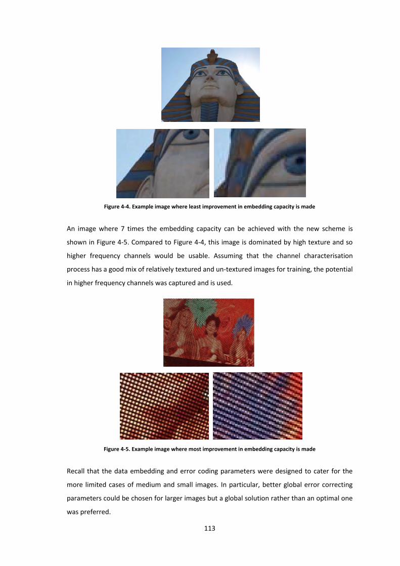
113
Figure 4-4. Example image where least improvement in embedding capacity is made
An image where 7 times the embedding capacity can be achieved with the new scheme is
shown in Figure 4-5. Compared to Figure 4-4, this image is dominated by high texture and so
higher frequency channels would be usable. Assuming that the channel characterisation
process has a good mix of relatively textured and un-textured images for training, the potential
in higher frequency channels was captured and is used.
Figure 4-5. Example image where most improvement in embedding capacity is made
Recall that the data embedding and error coding parameters were designed to cater for the
more limited cases of medium and small images. In particular, better global error correcting
parameters could be chosen for larger images but a global solution rather than an optimal one
was preferred.
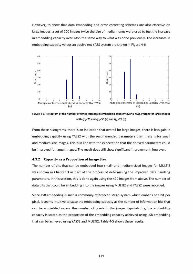
114
However, to show that data embedding and error correcting schemes are also effective on
large images, a set of 100 images twice the size of medium ones were used to test the increase
in embedding capacity over YASS the same way to what was done previously. The increases in
embedding capacity versus an equivalent YASS system are shown in Figure 4-6.
Figure 4-6. Histogram of the number of times increase in embedding capacity over a YASS system for large images
with =75 and =50 (a) and =75 (b)
From these histograms, there is an indication that overall for large images, there is less gain in
embedding capacity using YASS2 with the recommended parameters than there is for small
and medium size images. This is in line with the expectation that the derived parameters could
be improved for larger images. The result does still show significant improvement, however.
4.3.2 Capacity as a Proportion of Image Size
The number of bits that can be embedded into small- and medium-sized images for MULTI2
was shown in Chapter 3 as part of the process of determining the improved data handling
parameters. In this section, this is done again using the 400 images from above. The number of
data bits that could be embedding into the images using MULTI2 and YASS2 were recorded.
Since LSB embedding is such a commonly-referenced stego-system which embeds one bit per
pixel, it seems intuitive to state the embedding capacity as the number of information bits that
can be embedded versus the number of pixels in the image. Equivalently, the embedding
capacity is stated as the proportion of the embedding capacity achieved using LSB embedding
that can be achieved using YASS2 and MULTI2. Table 4-5 shows these results.
(a) (b)
1 2 3 4 5 6 7 8 9 100
10
20
30
40
50
60
Multiples of Increase In Embedding Capacity Over YASS
Occ
urr
ence
1 2 3 4 5 6 7 8 9 100
10
20
30
40
50
60
Multiples of Increase In Embedding Capacity Over YASS
Occ
urr
ence
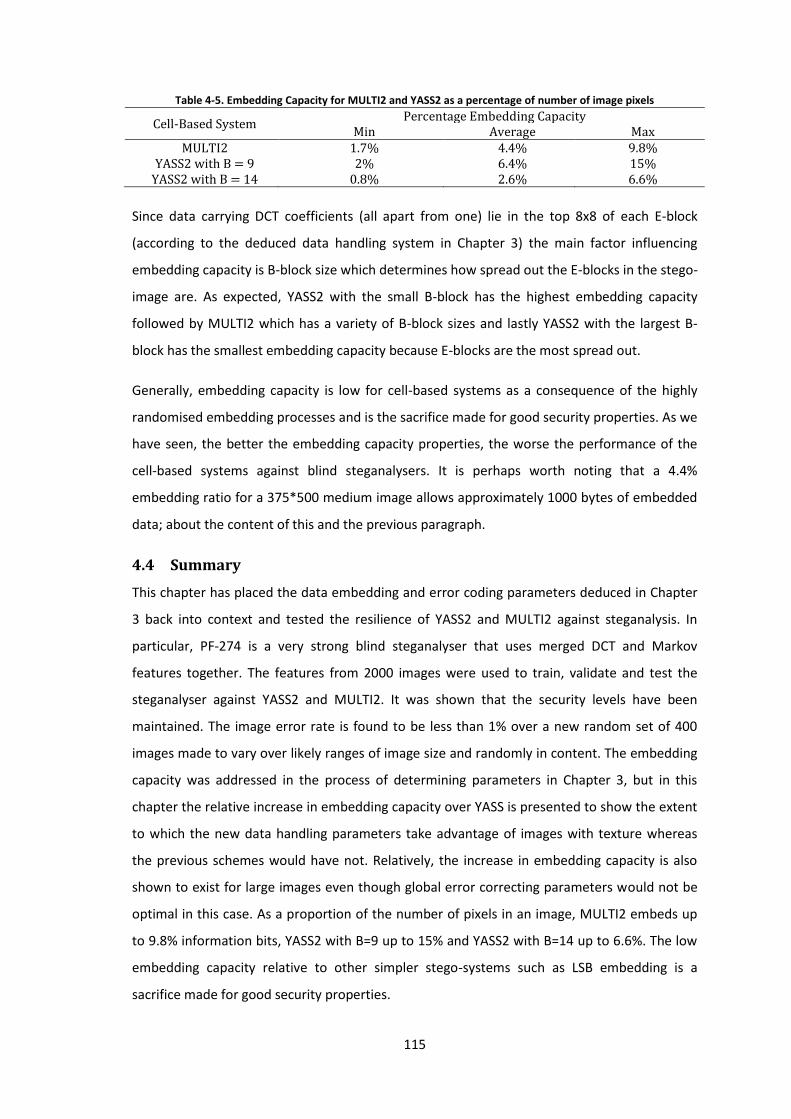
115
Table 4-5. Embedding Capacity for MULTI2 and YASS2 as a percentage of number of image pixels
Cell-Based System Percentage Embedding Capacity
Min Average Max MULTI2 1.7% 4.4% 9.8%
YASS2 with B = 9 2% 6.4% 15% YASS2 with B = 14 0.8% 2.6% 6.6%
Since data carrying DCT coefficients (all apart from one) lie in the top 8x8 of each E-block
(according to the deduced data handling system in Chapter 3) the main factor influencing
embedding capacity is B-block size which determines how spread out the E-blocks in the stego-
image are. As expected, YASS2 with the small B-block has the highest embedding capacity
followed by MULTI2 which has a variety of B-block sizes and lastly YASS2 with the largest B-
block has the smallest embedding capacity because E-blocks are the most spread out.
Generally, embedding capacity is low for cell-based systems as a consequence of the highly
randomised embedding processes and is the sacrifice made for good security properties. As we
have seen, the better the embedding capacity properties, the worse the performance of the
cell-based systems against blind steganalysers. It is perhaps worth noting that a 4.4%
embedding ratio for a 375*500 medium image allows approximately 1000 bytes of embedded
data; about the content of this and the previous paragraph.
4.4 Summary
This chapter has placed the data embedding and error coding parameters deduced in Chapter
3 back into context and tested the resilience of YASS2 and MULTI2 against steganalysis. In
particular, PF-274 is a very strong blind steganalyser that uses merged DCT and Markov
features together. The features from 2000 images were used to train, validate and test the
steganalyser against YASS2 and MULTI2. It was shown that the security levels have been
maintained. The image error rate is found to be less than 1% over a new random set of 400
images made to vary over likely ranges of image size and randomly in content. The embedding
capacity was addressed in the process of determining parameters in Chapter 3, but in this
chapter the relative increase in embedding capacity over YASS is presented to show the extent
to which the new data handling parameters take advantage of images with texture whereas
the previous schemes would have not. Relatively, the increase in embedding capacity is also
shown to exist for large images even though global error correcting parameters would not be
optimal in this case. As a proportion of the number of pixels in an image, MULTI2 embeds up
to 9.8% information bits, YASS2 with B=9 up to 15% and YASS2 with B=14 up to 6.6%. The low
embedding capacity relative to other simpler stego-systems such as LSB embedding is a
sacrifice made for good security properties.
116
Chapter 5. Conclusion
Cell-based systems have been shown to have good security properties at the cost of relatively
low embedding capacity. As part of the remedy for this, the data embedding and error coding
parameters for cell-based systems have been derived more analytically than in previous
literature, with the result that embedding capacity has indeed been improved.
Now that the main results of this research have been presented, this chapter gives an
overview of the flow of the dissertation and the most relevant points in each chapter. It is
intended to give the reader a terminating global view of the breadth and depth of work
explored in this dissertation. The extent to which the original research problem statement has
been addressed is also explained.
The chapter terminates with ideas for future research. The suggestions are concerned with
improving the results found here and addressing some assumed limitations on the stego-
systems.
5.1 Summary of Dissertation
5.1.1 Chapter 1
Chapter 1 starts by presenting an overview of the amount of media that is shared over the
Internet using facilities such as social media websites, blogs and emails. The sheer scale of the
online media-sharing culture and the ease with which content can be shared by almost anyone
has made security of transactions pertinent. In particular, steganography is introduced as a
mechanism for ensuring security and the prisoner’s problem is used to explain the main
elements of a stego-system. Steganography is defined as the science of hiding information in
innocent objects with the objective of avoiding suspicion from anyone viewing these objects.
The definition of steganography is further clarified by contrasting it with its sister concepts of
cryptography and watermarking.
Although relatively new in the digital domain, steganography can be traced back to the Golden
Age in Greece where it was used in conjunction with wax tablets to transmit secret
information. Since then, it was widely used in the 1900s during the wars. Some of the popular
examples of this are invisible inks and microdots. Until the 1900s, steganography was used
mainly by spies and involved clever tricks with little theoretical basis but given the transition of
communication to the digital domain it has experienced a renaissance to become a highly
technical and mathematical field. Since electronic communication is susceptible to
eavesdropping, security and privacy are more important than ever. Also given that digital
117
steganography may be used by criminals or terrorists or to carry malicious data such as viruses,
research into steganography is important also to be able to counteract this.
Steganography’s nemesis is steganalysis, which is the operation performed by the warden in
the passive situation where transactions are not tampered with. Within steganalysis, blind and
targeted approaches are possible. They differ according to the amount of information known
about the observed stego-system transactions a-priori and the extent to which the analyser
caters for a number of systems.
Steganography that uses digital images as covers (digital image steganography) is especially
relevant because digital images are the most popular form of media online. Digital images can
be represented in either compressed or uncompressed forms. Given the bandwidth limitations
on Internet connections, the compressed versions are more practical. In particular, JPEG
compression is the most popular form of compression online and therefore digital image
stego-systems should be designed to cater for this. A vital consideration is that JPEG
compression is lossy meaning the image data is corrupted during the compression process. If
data is embedded into an image before it undergoes compression then the compression
process tends to disguise embedding artefacts but error coding needs to be implemented to
correct for data corruption.
Within digital image steganography, cell-based systems cater for JPEG compression and have
very good security properties due to the random nature of embedding and the fact that
embedding is performed before compression. However, because the entire cover image is not
used to carry data and because error coding is required, cell-based systems have a particularly
low embedding capacity. Data embedding and error coding schemes in cell-based systems
have not been determined analytically in the literature previously and it is believed that these
schemes could be chosen more methodically with the consequence of improving embedding
capacity. This is presented as the primary research goal of this dissertation.
An overview of the research methodology is then given in steps – from first investigating the
field around cell-based systems and the context within which they were created, to defining a
new approach to determining data embedding and error coding schemes, to finally deducing
the schemes and testing them in the context of cell-based systems. The chapter ends with a
brief overview of the chapter contents.
118
5.1.2 Chapter 2
Chapter 2 focuses on digital image steganography specifically and starts by explaining the most
pertinent characteristics assumed for the stego-systems in this dissertation. In particular, a
public key, passive warden stego-system by cover modification is assumed because these
characteristics are the most popular in current literature. Following this, a formal flow chart of
the stego-system model is given along with relevant terminology.
The measures of success of stego-systems are defined- imperceptibility, capacity and
robustness. The three characteristics tend to counteract each other so no system can be found
that has all three excellent qualities. Out of them, imperceptibility is the most important. The
concept of visual imperceptibility is discussed, and the failings of the mean square error
measurement are shown. Given that media objects transmitted over the Internet are likely to
be displayed and seen, it would be foolish for any stego-system to introduce clear visual
artefacts. As a result, the battle between steganography and steganalysis has moved to the
more subtle statistical level. Embedding artefacts are determined by detecting statistical
discrepancies rather than visual ones. Given this transition from naïve to complex systems, the
term detectability is introduced to refer to the resistance of a system to statistical analysis
whereas imperceptibility is re-defined to be limited to the extent to which a stego-system does
not introduce visual embedding artefacts. Statistical properties regarding security are then
presented, including Cahin’s definition of security and the concept of a Ɛ-secure system.
The taxonomy of digital image steganography is then explained starting with naïve spatial
domain techniques. At this point in the report, the spatial representation of images is
explained and in particular intensity images are of interest. The concept of colour spaces and is
also described.
Within naïve digital steganography, two primary fields exist. The first is LSB embedding where
the LSB of the binary representation of the intensity of the pixels in an image are changed to
the secret message bits. While this does not cause any visual artefacts, analysis of the
statistical distribution of the LSB plane of the stego-image shows clear traces of tampering. If
bits other than the LSB are used for data hiding then visual defects may appear, known as the
bleeding effect. The second form of naïve steganography uses quantisation and dithering in
palette images but this usually results in visual artefacts and due to its limited applications is
not a popular research topic.
With regard to complex spatial domain stego-systems, the goal is generally to camouflage data
within an image so that natural statistical distributions are maintained. One example is to
119
attempt to mimic natural noise inserted into an image during image acquisition with a digital
camera. Another example is to aim to preserve some specific statistical property such as the
shape of an image histogram used usually by steganalysers. In particular, LSB embedding has
become popular as an adaptive scheme where data is hidden in select regions with more
texture and where more statistical redundancy exists. The topic of adaptive schemes is
discussed to some detail.
Although spatial domain techniques are still being investigated, the chapter describes how
they are not very useful because they do not cater for the likely possibility of an image being
JPEG compressed. The transform representation (DCT) and JPEG compression are then
described. The physical significance of the DCT and the properties of low and high frequency
components are given. In particular, it is shown that low frequency components are the most
significant part of an image visually and that high frequency components represent the detail
in an image. JPEG compression operates on the premise that the human visual system is
insensitive to detail in an image and thus works to remove high frequency DCT coefficients.
The lossy part of JPEG compression occurs with rounding after division by the corresponding
element from the quantisation matrix. Transform domain digital image stego-systems lend
themselves to accommodating lossy JPEG compression because JPEG involves generation and
manipulation of transform coefficients of an image. JPEG stego-systems such as Jsteg, F5 and
Outguess are then described.
The JPEG stego-systems explained up to this point embed data into images after the lossy
stage of compression and thus have not implemented error coding. The dissertation explains
that cell-based system has emerged as a transform-based system that embeds into the DCT
coefficients of an image before lossy JPEG compression. Instead of trying to camouflage
statistical artefacts of embedding, it attempts to disable a blind steganalyser’s ability to
estimate original cover image statistics by randomising data embedding. In particular, the
areas of the image used for data carrying are varied randomly.
The steps of YASS, the first cell-based system to appear in the literature, are then presented.
The concepts of blocking, RA coding and QIM are explained. YASS is also explained to embed
into the first 19 DCT coefficients of an E-block. In particular, the description of the delta values
using QIM in the literature is deferred to Chapter 4. Selection criteria and the rejection of the
DC coefficients from embedding are elaborated upon as requirements to prevent clear
statistical embedding artefacts. Extending on the ideas of YASS, the MULTI scheme was
presented which introduces two orders of increase in complexity of steganalysis over the
120
original YASS scheme by allowing variation of B-block and E-block sizes in an image. While the
cell-based systems have rigorously addressed security, the parameters of error coding, QIM
and the use of only the first 19 AC DCT coefficients in an E-block have not been analytically
determined.
Seeing the effect of JPEG compression on various coefficients, it becomes clear that correcting
for error across image blocks is not necessarily optimal since the data handling procedure
would be required to cater for a very wide range of error characteristics whereas a more
targeted approach would perform better. This idea plants the seed for the channel model
presented in the next chapter.
5.1.3 Chapter 3
Chapter 3 starts by explaining the main shortcomings of the traditional model of a channel as a
string of all of the DCT coefficients in all E-blocks sequentially. In particular, the range of errors
likely to be incurred will vary dramatically between low and high frequency DCT coefficients so
the data handling schemes would not be focused and efficient – they would either greatly
overcompensate in some places or undercompensate in others. A new channel model is
presented where an image is defined to contain many channels in parallel and where a
channel constitutes a string of all DCT coefficients from all E-blocks at a particular position
(frequency) in the E-Block. The idea behind this is that JPEG compression introduces a
particular grade of error to DCT coefficients of a particular frequency and so using the new
channel model, more targeted data handling procedures can be derived which are anticipated
to have a positive effect on embedding capacity.
The exact effects of JPEG compression on coefficient movement are then investigated. In the
case of JPEG-GRID the E-blocks and grid blocks used during JPEG compression are exactly
aligned and limits on the change in coefficient value due to JPEG compression can be
predicated precisely using the JPEG quantisation matrix. In the case of MULTI and YASS, this
cannot be done so precisely because E-blocks and JPEG compression grid blocks do not align,
although using a random sample of images the trend of increasing movement for higher
frequency channels is shown to still hold true.
Given the newly acquired knowledge regarding DCT coefficient movement, an explanation is
now given as to how data embedding parameters have been determined in cell-based systems
thus far. In the case of JPEG-GRID, the JPEG compression process can be rendered lossless by
using delta values corresponding to the JPEG quantisation matrix implemented during
compression and so JPEG quantisation matrices are used to provide delta values in YASS and
121
MULTI literature as a rough extension. Generally speaking, the delta matrix has a correct look
since delta values would be expected to be larger for higher frequency channels but in the case
of YASS or MULTI there is no obvious reason why this collection of delta values would be
optimal.
The concept of how delta relates to embedding capacity is then investigated. In particular, at
low delta, effects of higher error rate impact negatively on capacity whereas at high delta,
selection criteria impact negatively on embedding capacity. This leads to the idea that there
should be a moderate delta at which these factors combine optimally to produce maximum
embedding capacity. The target of the research is then defined to be the determination of the
plot of net embedding capacity versus delta for each channel from which data handling
parameters can be derived.
In order to plot embedding capacity versus delta, channel characteristics need to first be
determined. The most crucial of the characteristics are embedding rate (which represents the
proportion reduction in embedding capacity due to selection criteria) and error rate (which
represents the amount of error in the data carrying DCT coefficients that survive selection
criteria).
Since the characteristics regarding movement of YASS and MULTI cannot be determined
decisively as in the case of JPEG-GRID, the assumption is made that if measurements of
channel characteristics are made over a large enough number of images, eventually the
characteristics will converge and provide a good global representation. Deriving characteristics
in the most general case of MULTI will make characteristics applicable to all cell-based systems
since they all commonly involve simply generating random positions for DCT coefficients for
data carrying.
The main modules of the simulator are then expressed, and the assumption of =75 is
justified as the most commonly advertised JPEG quality factor in the literature. Using batches
of 100 coefficients, the channel characteristics are then determined as scatter plots of the
measurements.
To get an overview of the shape and trends in the scatter plots in order to detect convergence,
tolerance lines linking points below which a certain percentage of measurements exist are
drawn. These lines are analysed for movement over an ever-increasing number of images until
they stop moving.
122
Given the channel characteristics, if the effects of error coding are consolidated with them,
then the plot of embedding capacity versus delta can be generated and the point of maximum
embedding capacity can be read which provides the data embedding and error coding
parameters for optimal embedding capacity.
The exact nature of the error coding is then explored. In particular, if embedding is done in a
scattered fashion then random error correcting is appropriate. Additionally, the application
lends itself to block coding and BCH codes, which are particularly effective and flexible. Coding
should also be light since correcting for large amounts of error requires a high number of
overhead bits which doesn’t provide much benefit in terms of embedding capacity. The
simulator is edited appropriately to provide for channel-wise BCH coding scheme.
As a first step, channels with high error correcting requirements are rejected and from those
that remain plots of embedding capacity versus delta can be produced. It was found that 30
channels are usable per 12x12 E-block contradicting the assumption in previous literature that
only the first 19 channels are usable.
Since the error rate is required to be kept as low as possible, determination of the final
channel characteristics is delayed to consider further reducing image error rate. To cater for
any residual errors in the channels, this work designs for a global BCH code to keep image
error rate below the decided limit of 1%. In order to detect image errors, a light CRC code is
implemented. The global BCH code parameters are then matched for each possibility of error
rate tolerance level and the corresponding case of data handling parameters are generated. As
a result, there are now many possibilities of .
The choice between these parameters is made based on measurements of which combinations
of elements produced the best embedding capacity in small and medium images. This estimate
of likely size of cover images is made by analysing the popular image-sharing websites Flickr
and Facebook. Finally it was found that using an error tolerance of 98% with being 31 for
all channels gives the best embedding capacity and since it was derived for small- and
medium-sized images it would also apply for large images. A cell-based system that uses the
derived data handling systems is defined to be represented by a 2, as in YASS2 or MULTI2.
5.1.4 Chapter 4
Chapter 4 places the data handling parameters derived in Chapter 3 into context and measures
resistance of YASS2 and MULTI2 against steganalysis and image error rate requirements.
123
An explanation of detection rate and the operation of a powerful blind steganalysis scheme,
PF-274, is given. Out of all blind steganalysers, PF-274 has been found to be the most effective
in detecting YASS and combines DCT and Markov measurements as features used to train a
neural network. The results show that security requirements continue to be met. There is an
elevation in detection rate in 1% for YASS and MULTI with the new data handling parameters
but this is probably due to slightly elevated delta values for low frequency channels.
Image error rate is then tested by embedding data into 400 images of varying size and
checking the number of images in error manually and using the CRC code. The image error rate
was found to be 0.75% meeting the original requirements of 1%. In addition, the CRC code
correctly identified the erroneous image.
Since cell-based parameters originally didn’t attempt to address data handling systems
rigorously, directly comparing the new parameters with the old ones does not make a
powerful point but it does show that a steganographer can achieve better embedding capacity
using the new data handling systems than previously. Using an optimistic RA coding rate of 10,
the two systems are compared in the case of YASS for small and medium –sized images and
significant improvement is shown. The images for which the worst (2x) and best (7x)
improvement is made are analysed and it is found that the best improvement is made where
an image is highly textured and the worse for where the image is lightly textured. This shows
that there is benefit in using more vulnerable channels than just the first 19 as used by YASS
originally. The same experiment is repeated for large images and while improvements are not
as large due to the global error correcting parameters not being optimal, there is still
significant benefit.
As a proportion of the number of pixels in an image, MULTI2 embeds up to 9.8% information
bits, YASS2 with B=9 up to 15% and YASS2 with B=14 up to 6.6%. The low embedding capacity
relative to other simpler stego-systems such as LSB embedding is a sacrifice made for good
security properties.
5.2 Concluding Comments
The original goal for this research was to investigate an approach to determining data
embedding and error correcting schemes more analytically than has been done before in the
literature with the aim of increasing embedding capacity in cell-based systems while
maintaining good security properties. This dissertation has presented such an approach and
deduced data handling schemes such that a low image error rate and good embedding
124
capacity can be achieved over all expected image contents and sizes. It can be concluded then
that the original goals were met in their entirety.
5.3 Future Work
Any future work will address limitations in the results of this research to provide further
improvement in embedding capacity and security. Some suggestions are:
1. Generate a technique that selects the parameters for data embedding and local and
global error correcting adaptively based on a given cover-image so that these processes
are optimised. This would also require the adaptive parameters to be somehow
communicated to the intended recipient which could be performed by embedding them
in a standard way in more reliable areas of an image.
2. Address the scenario where not of all of the space in a cover image is used for data
carrying, i.e. where embedding capacity is less than 100%. This work would address the
best way to distribute data around the image to ensure security, and would provide
provision for some sort of aggression level for embedding.
3. QIM could be used to embed symbols rather than individual bits to increase embedding
capacity. The details of how to do this would still need to be addressed.
4. By taking the approach presented here, comparing the effectiveness and suitability of
various error correcting schemes (versus only using BCH codes) could be analysed.
5. Instead of accepting the elevated delta values for low frequency channels as in Chapter 4,
the extent to which lowering them to sub-optimal points for security purposes could be
explored.
125
References
JPEG. (2007). Retrieved November 2011, 19, from JPEG Homepage:
http://www.jpeg.org/jpeg/index.html
The President Elect’s Favorite Movies and Books. (2008, November 24). Retrieved April 6, 2011,
from Dublin Library: http://dublinlibrary.wordpress.com/2008/11/
cat + blanket - created by cocor . (2010). Retrieved April 6, 2011, from pixleyes.com:
http://www.pxleyes.com/photography-picture/4d6392d1ecb42/cat---blanket.html
ReadWrite Cloud. (2010, August 10). Retrieved April 2, 2011, from How Facebook Scales with
Open Source: http://www.readwriteweb.com/cloud/2010/08/how-facebook-scales-with-
open.php
Rst. (2010). Retrieved April 5, 2011, from Earth System Science, Mission to Planet Earth, and
the Earth Observing System: http://rst.gsfc.nasa.gov/Sect16/Sect16_1.html
Answers.com. (2011). Retrieved April 2, 2011, from How many pictures are uploaded onto
facebook every second?:
http://wiki.answers.com/Q/How_many_pictures_are_uploaded_onto_facebook_every_secon
d
JPEG. (2011, November 22). Retrieved April 6, 2011, from Wikipedia:
http://en.wikipedia.org/wiki/JPEG
Anderson, R. (1996). Information Hiding: First International Workshop. Berlin: Springer-Verlag.
Beaullieu, S., Crissey, J., & Smith, I. (2000). Retrieved April 5, 2011, from BPCS Steganography:
http://www.ianrichard.com/bpcs/abstract.pdf
Braga, M. (2010, July 28). Tested. Retrieved November 2011, 19, from JPEG and You: How the
Most Popular Photo Format Works: http://www.tested.com/news/jpeg-and-you-how-the-
most-popular-photo-format-works/614/
Brassil, J., Low, S., Maxemchuk, N., & O'Gorman, L. (1995). Hiding information in document
images. Proceedings of the Conference on Information Sciences and Systems, CISS (pp. 482-
489). Baltimore: John Hopkins University.
Brewster, D. (1857). Microscope, volume XIV. Encyclopedia Britannica or the Dictionary of Arts,
Sciences, and General Literature - Application of photography to the microscope. Edinburgh.
126
Cahin, C. (2004). An information-theoretic model for steganography. Information and
Computation, Vol. 192(1), 41-56.
Chandramouli, R., & Subbalakshmi, K. (2003). Active steganalysis of spread spectrum image
steganography. Proceedings of the 2003 International Symposium on Circuits and Systems,
2003. ISCAS’03, volume 3, (pp. III-830 - III-833). Hoboken.
Cheddad, A., Condell, J., Curran, K., & McKevitt, P. (2010). Digital image steganography: Survey
and analysis of current methods. Signal Processing, 727-752.
Chen, B., & Wornell, G. (2011, May 4). Quantization Index Modulation: A Class of Provably
Good Methods for Digital Watermarking and Information Embedding. IEEE Transactions on
Information Theory, pp. 1423-1443.
Cole, E., & Krutz, R. (2003). The Growth of Steganography. In E. Cole, & R. Krutz, Hiding in Plain
Sight. Steganography and the Art of Covert Communication (pp. 53-54). Indianapolis: Wiley
Publishing, Inc.
Dabeer, O., Sullivan, K., Madhow, U., Chandrasekaran, S., & Manjunath, B. (2004). Detection of
hiding in the least significant bit. IEEE Transactions on Signal Processing, Supplement on
Secure, 3046–3058.
Dawoud, P. (2010). An Improved Randomisation of a Multi-Blocking JPEG Based
Steganographic System. M.Sc. Thesis.
Debattista, K. (2010, January 11). TalkTechToMe. Retrieved November 24, 2011, from The
Threats of Steganogrphy: http://www.gfi.com/blog/threats-steganography/
Facebook. (2011, November 18). Facebook. Retrieved November 18, 2011, from Statistics:
https://www.facebook.com/press/info.php?statistics
Fan, K., & Wediong, K. (2004). A Secure Steganography Scheme Based on (N,t) Threshold. 18th
International Conference on Advanced Information Networking and Applications (p. 536).
Fukouka: AINA.
Franz, E., & Schneidewind, A. (2005). Pre-processing for adding noise steganography.
Information Hiding, 7th International Workshop (pp. 189-203). Barcelona: Springer-Verlag.
(2010). In J. Fridrich, Steganography in Digital Media: Principles, Algorithms, and Applications
(pp. 83-85). New York: Cambridge University Press.
127
Fridrich, J. (2010). Introduction. In J. Fridrich, Steganography in Digital Media - Principles,
Algorithms, and Application (pp. 6-7). New York: Cambridge University Press.
Fridrich, J. (2010). Steganographic Channel. In J. Fridrich, Steganography in Digital Media:
Principles, Algorithms and Applications (pp. 50-56). New York: Cambridge University Press.
Fridrich, J., & Du, R. (1999). Secure Steganographic Methods for Palette Images. Information
Hiding: Third International Workshop (pp. 47-60). Dresden: Springer-Verlag.
Fridrich, J., & Goljan, M. (2002). Practical Steganalysis - State of the Art. Security and
Watermarking of Multimedia Contents, vol. 4675, 1-13.
Fridrich, J., & Goljan, M. (2003). Digital Image Steganography Using Stochastic Modulation.
Proceedings SPIE, Electronic Imaging, Security and Watermakring of Multimedia Contents V
(pp. 191-202). Santa Clara: Springer-Verlag.
Fridrich, J., & Kodovsky, J. (2008). Influence of Embedding Strategies on Security of
Steganographic Methods in the JPEG Domain. SPIE, Electronic Imaging, Security, Forensics,
Steganography, and Watermarking of Multimedia Contents X, volume 6819 (pp. 200-213). San
Jose, CA: SPIE.
Fridrich, J., Goljan, M., & Hogea, D. (2003). Steganalysis of JPEG Images: Breaking the F5
Algorithm. Petitcolas, F.A.P. (Ed.): Inf. Hiding: 5th Intl. Workshop. LNCS, 2578 (pp. 310-323).
Berlin: Springer-Verlag.
Fridrich, J., Goljan, M., Lisoňek, P., & Soukal, D. (2004). Writing on wet paper. ACM Workshop
on Multimedia and security. Magdeburg, Germany.
Fu, D., Shi, Y., Zou, D., & Xuan, G. (2006). JPEG Steganalysis Using Empirical Transition Matrix in
Block DCT Domain. IEEE 8th Workshop on Multimedia Signal Processing, (pp. 310-313).
Victoria.
Gonzalez, R., & Woods, R. (2002). Image Types. In R. Gonzalez, & R. Woods, Digital Image
Processing Using Matlab (pp. 24-14). New Jersey: Prentice Hall, Inc.
Gonzalez, R., & Woods, R. (2002). JPEG. In R. Gonzalez, & W. RE, Digital Image Processing
Using Matlab (pp. 318-321). New Jersey: Prentice Hall, Inc.
128
Gordhamer, S. (2009, October 16). Mashable. Retrieved November 18, 2011, from 5 Ways
Social Media is Changing Our Daily Lives: http://mashable.com/2009/10/16/social-media-
changing-lives/
Guo, J.-M., & Le, T.-N. (2010). Secret Communication Using JPEG Double Compression. IEEE
Signal Processing Letters, Vol. 17, No. 10, 879-882.
Hackersdelight.org. (2009, 7 28). Hackersdelight. Retrieved November 20, 2011, from CRC:
http://www.hackersdelight.org/crc.pdf
Hass, C. (2008). Impulse Adventure. Retrieved 11 1, 2011, from JPEG Compression, Quality and
File Size: http://www.impulseadventure.com/photo/jpeg-compression.html
Hedieh, S., & Jamzad, M. (2008). Cover Selection Steganography Method Based on Similarity of
Image Blocks . IEEE 8th International Conference on Computer and Information Technology
Workshops, 2008. CIT Workshops 2008, (pp. 379-384 ). Jeju.
Hedieh, S., & Jamzad, M. (2010). BSS: Boosted steganography scheme with cover image
preprocessing. Expert Systems with Applications, 7703–7710.
Herodotus. (1992). The Histories. In Herodotus, The Histories (pp. Chapter 5 - Terpischore).
New York: J.M. Dent & Sons, Ltd.
Hetzl, S., & Mutzel, P. (2005). A graph theoretic approach to steganography. 9th IFIP TC-6 TC-
11 International vol. 3677, (pp. 119–128). Salzburg.
Hetzl, S., & Mutzel, P. (2005). A graph-theoretic approach to steganography. In Lecture Notes
in Computer Science (pp. 119-125). Bath: Springer.
Hsiao, J.-Y., & Chang, C.-T. (2011). An adaptive steganographic method based on the
measurement of just noticeable distortion profile. Image and Vision Computing, 155-166.
Huang, F., Huang, J., & Qing Shi, Y. (2010). An Experimental Study on the Security Performance
of YASS. IEEE Transactions on Information Forensics and Security, Vol. 5, No. 3, 374-491.
Huang, F., Huang, J., & Shi, Y. Q. (2010). An Experimental Study on the Security Performance of
YASS. IEEE Transactions on Information Forensics and Security, Vol. 5, No. 3, 374-491.
Johnson, N., & Sallee, P. (2008). Detection of hidden information, covert channels and
informations flows. In J. Voeller (Ed.), Wiley Handbook of Science Technology for Homeland
Security (pp. 20-22). New York: Wiley & Sons, Inc.
129
Kahn, D. (1996). The Rise of the West. In D. Kahn, The Code Breakers - The Comprehensive
History of Secret Communication from Ancient Times to the Internet (pp. 106-125). New York:
Scribner.
Kawaguchi, E., & Eason, E. (1998). Principle and Applications of BPCS-Steganography.
Proceedings SPIE, (pp. 464-473). Beijing.
Kerckhoffs, A. (1883). La Cryptographie Militaire. Journal des Sciences Militaires, Vol. IX, 5-83.
Kermani, Z., & Jamzad, M. (2005). A robust steganography algorithm based on texture
similarity using gabor filter. Proceeding of IEEE international symposium signal processing and
information technology, (pp. 578–582). Athens.
Kharrazi, M., Sencar, H., & Memon, N. (2006). Cover Selection for Steganographic Embedding.
Proceedings of the International Conference on Image Processing, (pp. 117-120). Atlanta.
Kumar, K., Raja, K., Chhotaray, R., & Pattnaik, S. (2010). Coherent steganography using
Segmentation and DCT. 2010 IEEE International Conference on Computational Intelligence and
Computing Research (ICCIC), (pp. 1 - 6). Coimbatore.
Kuo, S.-M., Lee, B., & Tian, W. (2006). Cyclic Redundant Code. In S.-M. Kuo, B. Lee, & W. Tian,
Real-Time Digital Signal Processing: Implementations and Applications (p. 563). West Sussex:
John Wiley & Sons.
Li, B., Huang, J., & Shi, Y. Q. (2009). Steganalysis of YASS. IEEE Transactions on Information
Forensics and Security, Vol. 4, No. 3, 369-382.
Lin, E., & Delp, E. (1999). A review of data hiding in digital images. Proceedings of the Image
Processing, Image Quality, Image Capture Systems Conference, PICS'99, (pp. 274-278).
Savannah.
Lin, K. T. (2011). Hybrid encoding method by assembling the magic-matrix scrambling method
and the binary encoding method in image hiding. Optics Communications, 1778–1784.
Lin, S., & Costello, D. (1983). Types of Codes. In A. Simpson (Ed.), Error Control Coding:
Fundamentals and Applications (pp. 3-5). Englewood Cliffs: Prentice-Hall, Inc.
Luo, W., Huang, F., & Huang, J. (2010). Edge Adaptive Image Steganography Based on LSB
Matching Revisited. IEEE Transactions on Information Forensics and Security, Vol. 5, No. 2, 201-
214.
130
MathWorks. (2011). MathWorkd. Retrieved November 29, 2011, from Neural Network
Toolbox: http://www.mathworks.com/products/neural-network/index.html
MathWorks. (2011). R2011b Documentation - Communications System Toolbox. Retrieved
November 29, 2011, from bchenc:
http://www.mathworks.com/help/toolbox/comm/ref/bchenc.html
MathWorks. (2011). R2011b Documentation - Communications System Toolbox. Retrieved
November 29, 2011, from bchdec:
http://www.mathworks.com/help/toolbox/comm/ref/bchdec.html
MathWorks. (2011). R2011b Documentation - Communications System Toolbox. Retrieved
November 29, 2011, from comm.CRCGenerator class:
http://www.mathworks.com/help/toolbox/comm/ref/comm.crcgeneratorclass.html
McCullagh, D. (2001, February 7). Wired. Retrieved November 29, 2011, from Bin Laden:
Steganography Master?:
http://www.wired.com/politics/law/news/2001/02/41658?currentPage=all
Mielkainen, J. (2006, May). LSB matching revisited. IEEE Signal Processing Letters, Vol. 13, No.
5, pp. 285-287.
Naughton, J. (2010, August 15). The Guardian. Retrieved November 18, 2011, from The
internet: is it changing the way we think?:
http://www.guardian.co.uk/technology/2010/aug/15/internet-brain-neuroscience-debate
Negrat, K., Smko, R., & Almarimi, A. (2010). Variable length encoding in multiple frequency
domain steganography. 2010 2nd International Conference on Software Technology and
Engineering (ICSTE), (pp. 305-309). Kuala Lumpur.
Pevny, T., & Fridrich, J. (2006). Multi-Class Blind Steganalysis for JPEG Images. Proceedings of
SPIE (pp. 1-13). San Jose: SPIE.
Pevny, T., & Fridrich, J. (2007). Merging Markov and DCT Features for Multi-Class JPEG
Steganography. Proceeding of SPIE, (pp. 3-4). San Jose.
Pfitzmann, B., & Anderson, R. (1996). Information hiding terminology. Information Hiding: First
International Workshop (pp. 347-350). Cambridge: Springer-Verlag.
131
Proakis, J., & Salehi, M. (2002). Coefficients of the Generator Polynomials of BCH Codes. In J.
Proakis, & M. Salehi, Communication Systems Engineering Second Edition (pp. 621-622). Upper
Saddle River: Prentice-Hall, Inc.
Provos, N. (2000). Defending against statistical steganalysis. 10th USENIX Security Symposium,
Washington DC, USA of the IEEE 22nd Annual EMBS International Conference, (pp. 280-283).
Chicago.
Rockwell, K. (2007, June 1). KenRockwell.com. Retrieved November 2011, 19, from How We
See: http://www.kenrockwell.com/tech/how-we-see.htm
Rosenberg, M. (2011, May 11). About.com Geography. Retrieved November 18, 2011, from
Most Populous Countries Today:
http://geography.about.com/cs/worldpopulation/a/mostpopulous.htm
Sajedi, H., & Jamzad, M. (2008). Cover Selection Steganography Method Based on Similarity of
Image Blocks. IEEE 8th International Conference on Computer and Information Technology
Workshops, (pp. 379-384). Sydney.
Sajedi, H., & Jamzad, M. (2010). HYSA: HYbrid Steganographic Approach using multiple
steganography methods. Retrieved March 24, 2011, from Wiley Online Library:
wileyonlinelibrary.com
Sallee, P. (2003, September). Retrieved June 1, 2011, from Matlab JPEG Toolbox:
http://www.philsallee.com/jpegtbx/index.html
Sallee, P. (2004). Model-based steganography. In T. Kalker, I. Cox, & Y. Ro, LNCS, vol. 2939 (pp.
154–167). Heidelberg: Springer.
Sarkar, A., Nataraj, L., Manjunath, B., & Madhow, U. (2008). Estimation of Optimum Coding
Redundancy and Frequency Domain Analysis of Attacks for YASS - A Randomised Block Hiding
Scheme. 15th IEEE International Conference on Image Processing, ICIP 2008. (pp. 1292 - 1295).
San Diego, CA: IEEE.
Sarkar, A., Solanki, K., & Manjunath, B. (2008). Further study on YASS: steganography based on
randomized embedding to resist blind steganalysis. Proc. Electronic Imaging, Security,
Forensics, Steganography, and Watermarking of Multimedia Contents X. San Jose: SPIE.
Schaefer, G., & Stich, M. (2004). UCID - An Uncompressed Colour Image Database. Storage and
Retrieval Methods and Applications for Multimedia (pp. 472-480). San Jose: SPIE.
132
Shi, Y., Chen, C., & Chen, W. (2006). A Markov Process Based Approach to Effective Attacking
JPEG Steganography. 8th Information Hiding Workshop. Old Town Alexandria.
Simmons, G. (1984). The prisoner's problem and subliminal channel. Advances in Cryptology,
Proceedings of CRYPTO (pp. 51-67). CRYPTO.
Smith, J., & Comiskey, B. (1996, Moay). Modulation and Information Hiding in Images.
Springer-Verlag Lecture Notes in Computer Science, pp. 207-226.
Solanki, K., Jacobsen, N., Madhow, U., Manjunath, B., & Chandrasekaran, S. (2004, December).
Robust Image-Adaptive Data Hiding Using Erasure and Error Correction. IEEE Transactions on
Image Processing, Vol. 13, No. 12, pp. 1627-1639.
Solanki, K., Sarkar, A., & Manjunath, B. (2007, June). YASS: yet another steganographic scheme
that resists blind from 9th International Workshop on Information Hiding. Information Hiding:
9th International Workship, (pp. 16-31). Saint Malo.
Solanki, K., Sullivan, K., Madhow, U., Manjunath, B., & Chandrasekaran, S. (2005). Statistical
restoration for robust and secure. Proc. ICIP, (pp. II 1118–1121). Genova.
Solanki, K., Sullivan, K., Madhow, U., Manjunath, B., & Chandrasekaran, S. (2006). Probably
secure steganography: Achieving zero K-L divergence using statistical restoration. Proc. ICIP,
(pp. 125–128). Atlanta.
Stanescu, D., Stangaciu, V., & Stratulat, M. (2010). Steganography on new generation of mobile
phones with image and video processing abilities. 2010 International Joint Conference on
Computational Cybernetics and Technical Informatics (ICCC-CONTI), (pp. 343-347 ). Timisoara.
Statsr.net. (2011, 6 10). Statsr.net. Retrieved November 20, 2011, from Flickr Stats:
http://statsr.net/flickr-stats/
Su, P.-C., & Kuo, C.-C. J. (2003). Steganography in JPEG2000 Compressed Images. IEEE
Transactions on Consumer Electronics, Vol. 49, No. 4, 824-832.
Sullivan, K., Madhow, U., Chandrasekaran, S., & Manjunath, B. (2006, February). Steganalysis
for Markov Cover Data with Applications to Images. IEEE Transactions on Information Forensics
and Security, pp. 275-287.
133
Sun, Q., Qiu, Y., Ma, W., Yan, W., & Dai, H. (2010). Image Steganography Based on Sub-Band
Coefficient Adjustment in BDCT Domain . 2010 International Conference on Multimedia
Technology (ICMT), (pp. 1-4 ). Ningbo.
Tseng, Y.-C., Chen, Y.-Y., & Pan, H.-K. (2002). A Secure Data Hiding Scheme for Binary Images.
IEEE Transactions on Communications, Vol. 50, No. 8, 1227-1231.
Upham, D. (1993). Retrieved March 5, 2011, from JPEG–Jsteg:
http://zooid.org/~paul/crypto/jsteg/
Vaudenay, S. (2002, July 15). LASEC - Security and Cryptography Laboratory. Retrieved 12 15,
2011, from Introduction to Decorrelation Theory:
http://lasecwww.epfl.ch/memo/dec_manual.shtml
Velasco, C., Nakano, M., Perez, H., Martinez, R., & Yamaguchi, K. (2009). Adaptive JPEG
steganography using convolutional codes and synchronization bits in DCT domain. 52nd IEEE
International Midwest Symposium on Circuits and Systems, 2009. MWSCAS '09, (pp. 842-847).
Cancun.
Weisstein, E. (2011). MathWorld-A Wolfram Web Resource. Retrieved November 29, 2011,
from Markov Process: http://mathworld.wolfram.com/MarkovProcess.html
Westfeld, A. (2001). High capacity despite better steganalysis (F5-a steganographic algorithm).
Information Hiding. LNCS, vol. 2137, pp. 289–302.
Westfeld, A., & Pfitzmann, A. (1999). Attacks on Steganographic Systems. Information Hiding,
3rd International Workshop (pp. 61-75). Dresden: Springer-Verlag.
Wilkins, E. (1954). A History of Italian Literature. London: Oxford University Press.
Xiaoyi, Y., & Babaguchi, N. (2008). Breaking the YASS algorithm via pixel and DCT coefficients
analysis. 19th International Conference on Pattern Recognition, 2008. ICPR 2008, (pp. 1-4).
Florida.
Yang, C.-H., Weng, C.-Y., Tso, H.-K., & Wang, S.-J. (2011). A data hiding scheme using the
varieties of pixel-value differencing in multimedia images. The Journal of Systems and
Software, 669-678.
Yeung, M., & Yeo, B. (1998, February 11). Fragile Watermarking of Three Dimensional Objects.
IEEE Computer Society, pp. 442-446.

134
Yu, L., Zhao, Y., Ni, R., & Shi, Y. (2010). A high-performance YASS-like scheme using randomized
big-blocks . 2010 IEEE International Conference on Multimedia and Expo (ICME), (pp. 474-479 ).
Singapore.


![Steganographic Watermarking for Documents - CNC · Steganographic Watermarking for Documents Benjamín Barán, Santiago Gómez and Víctor Bogarín Email: [bbaran, vbogarin]@cnc.una.py](https://static.cupdf.com/doc/110x72/5b48ed9b7f8b9aa4148dcad3/steganographic-watermarking-for-documents-steganographic-watermarking-for.jpg)