Observability of Flow-Dependent Structure Functions for Use in Data Assimilation
CRISTINA LUPU AND PIERRE GAUTHIER
Department of Earth and Atmospheric Sciences, Universite du Quebec a Montreal, Montreal, Quebec, Canada
(Manuscript received 18 March 2010, in final form 19 October 2010)
ABSTRACT
One of the objectives of data assimilation is to produce initial conditions that will improve the quality of
forecasts. Studies on singular vectors and sensitivity studies have shown that small changes to the initial
conditions can sometimes lead to exponential error growth. This has motivated research to include flow-
dependent structures within the assimilation that would have the characteristics to correctly predict the
growth or decay of meteorological systems. This relates to the characterization of precursors to atmospheric
instability. In this paper, the observability of such structures by observations is discussed. Several studies have
shown that deploying observations over regions where changes in the initial conditions may impact the
forecast the most do not lead to the expected benefit. In this paper, it is shown that given the small magnitude
of the signal to be detected, it is important to take into account the accuracy of the observations. If the signal-
to-noise ratio is too low, observations cannot detect and characterize precursors to forecast error growth.
From that perspective, the assimilation only has the possibility to extract information about evolved struc-
tures of error growth. Experiments with a simple one-dimensional variational data assimilation (1D-Var)
system are presented and, then, an adapted three-dimensional variational data assimilation (3D-Var) system
with different sensitivity structure functions is used. The results have been obtained by adapting the varia-
tional assimilation system of Environment Canada.
1. Introduction
The accuracy of analyses produced by data assimila-
tion systems depends on the precision of background
and observation error covariances specified as input.
The modeling and estimation of these covariances is
critical for any data assimilation system in the context of
numerical weather prediction (NWP). Algorithms like the
three-dimensional variational data assimilation (3D-Var)
produce analyses by blending together observations near
the analysis time with a background state provided by
a short-term numerical weather prediction. In this case,
the background-error statistics are taken to be stationary
and do not reflect the flow dependency of error growth
that depends on the particular meteorological situation.
Flow-dependent covariances can be obtained from ap-
proximate forms of the Kalman filter like the ensemble
Kalman filter (Evensen 1994; Houtekamer et al. 2009).
Instabilities in atmospheric flows can be triggered by
small perturbations to initial conditions and these can be
characterized using adjoint methods that enable us to
trace back the source of errors in a forecast to errors in
the analysis. Lacarra and Talagrand (1988) showed that
it is possible to characterize the structure of perturba-
tions to the initial conditions that would lead to the most
significant growth over a finite period of time. Those
correspond to the so-called singular vectors that define
the unstable subspace containing those perturbations
that will experience the most significant error growth.
This has been the foundation of the design of ensemble
prediction systems that aim to determine how errors in
the analysis and the model will lead to forecast errors
in the medium range (Molteni et al. 1996; Buizza et al.
2007a).
Since it is possible to characterize those regions where
perturbations in the analysis can lead to important error
growth, the next logical step was to use this information
to deploy observations in those areas where a reduction
in the analysis error could lead to the most important
reduction of the forecast error. This is the basis of tar-
geting methods, which use information from singular
vector or sensitivity gradients to plan the deployment of
Corresponding author address: Cristina Lupu, European Centre
for Medium-Range Weather Forecasts, Shinfield Park, Reading,
RG2 9AX, United Kingdom.
E-mail: [email protected]
VOLUME 139 M O N T H L Y W E A T H E R R E V I E W MARCH 2011
DOI: 10.1175/2010MWR3424.1
� 2011 American Meteorological Society 713
adaptive observations. The Fronts and Atlantic Storm
Track Experiment (FASTEX) campaign (Joly et al. 1999)
was the first to test targeting methods and observations
were deployed according to sensitivity gradients. Other
campaigns followed like the North Pacific Experiment
(NORPEX; Langland et al. 1999), the 2003 Atlantic The
Observing System Research and Predictability Experiment
(THORPEX) Regional Campaign (ATReC; Petersen
and Thorpe 2007; Langland 2005a) and recently, the 2008
THORPEX Pacific-Asia Regional Campaign (T-PARC).
From all those campaigns, the conclusions are that the
impact of observations deployed over sensitive areas in
the extratropics identified from singular vectors is, on
average, about twice that of any other single observa-
tion, but the overall impact is small because of the large
volume of data now assimilated (Langland 2005b; Kelly
et al. 2007; Buizza et al. 2007b; Cardinali et al. 2007).
These results bring us to reconsider the value of ex-
pensive observation campaigns for the sole purpose of
assessing if targeted observations do lead to significant
reduction of the forecast error. The current wisdom is
that, if observations are to be deployed, it is then ap-
propriate to take into account sensitivity information to
do it. Particularly, this may be valuable for adaptive data
selection for satellite data. Currently, because of limita-
tions in the assimilation systems, a small fraction of the
incoming volume of satellite data can be assimilated (Liu
and Rabier 2002). Adaptive data selection is now being
considered to assess whether this results in improvements
in the quality of forecasts.
Fisher and Andersson (2001) have proposed a reduced-
rank Kalman filter (RRKF) that restricts the evolution
of the background-error covariances within an unstable
subspace spanned by singular vectors. Their experimen-
tation was thorough and went all the way to include the
RRKF to provide the background-error covariances for
the European Centre for Medium-Range Weather Fore-
casts (ECMWF) four-dimensional variational data assim-
ilation (4D-Var). This was found to lead to a positive but
small impact on the resulting forecasts, which was not
deemed significant enough to implement this approach
in the ECMWF operational suite. Currently, hybrid ap-
proaches have been proposed in which ensemble methods
are used to define a subspace that is appropriate to de-
scribe the evolved background-error covariances (Buehner
et al. 2010a,b; Berre et al. 2009). The preliminary results
are very positive and this has sparked a renewed interest
to include flow-dependent background-error covariances
when cycling a 4D-Var assimilation system.
This paper’s objective is to investigate some issues
associated with the use of sensitivity information in the
representation of background-error covariances with a
3D-Var assimilation system. Hello and Bouttier (2001)
did propose an approach through which a priori sensi-
tivity information from a single singular vector was in-
cluded within the background-error covariance matrix,
denoted by B. Their approach is called an adapted
3D-Var as it includes some flow dependency. The a priori
sensitivity was used to deploy targeted data during the
FASTEX campaign (Hello et al. 2000). In the present
paper, a variant of their algorithm is presented and tested
both in a simple one-dimensional variational data assim-
ilation (1D-Var) context and in 3D-Var. The rationale on
which this study is based is the following.
The 24- or 48-h forecast error can be evaluated by
comparing it with respect to a verifying analysis, and the
adjoint of the forecast model can be used to define the
change in initial conditions that would reduce the fore-
cast error. This is referred to as key analysis errors, a
term coined by Klinker et al. (1998) and has been the
object of several studies afterward (Laroche et al. 2002;
Langland et al. 2002; Caron et al. 2007a). This will be
referred to as an a posteriori sensitivity function because
it can only be obtained as a diagnostic of the origin of
forecast error. In addition, a priori structure functions
defined either as leading singular vectors (SVs) or from
the gradient sensitivity vector method (Hello et al. 2000)
are tools that have been widely applied in sensitivity
studies, particularly for the development of targeting
techniques. In the gradient sensitivity vector method,
the cost function can be defined with respect to a par-
ticular aspect of the forecast at a later time and then to
find out what are the changes to the initial conditions
that will have the greatest impact on the forecast er-
ror growth. For example, taking the average of surface
pressure of a 24-h forecast over an area of interest, one
can then identify areas where changes in the current
analysis could have a significant impact as defined by the
sensitivity cost function. In Hello et al. (2000), this has
been used to identify those regions where small changes
to the initial conditions can be expected to lead to sub-
stantial changes in the forecast.
If a posteriori key analyses, as proposed by Klinker
et al. (1998), do result in a dramatic reduction of forecast
error, it would make sense to use those as structure
functions within the B matrix so that observations would
be used to define its amplitude. What was expected is that
the amplitude of the key analysis would be recovered.
However, this is not what happened. On second thought,
the signal that was to be recovered was very small, which
raised the question whether those structures could be
detected at all by the observations, which contain some
amount of observation error.
The paper is organized as follows. Section 2 briefly
presents the formulation of the variational 3D-Var data
assimilation system and its adapted 3D-Var version.
714 M O N T H L Y W E A T H E R R E V I E W VOLUME 139
Section 3 presents the assimilation in the subspace span-
ned by a single sensitive direction. A particular point con-
cerns the observability of a structure function defined from
a posteriori sensitivity. Results with a simple 1D-Var
model are presented in section 4 to illustrate the new
approach. Section 5 introduces different a posteriori sen-
sitivity structures chosen for this work and results based
on adapted 3D-Var experiments are described in sec-
tion 5. Finally, section 6 summarizes the results and pres-
ents some conclusions.
2. Flow-dependent structure functions in 3D-Var:The adapted 3D-Var
When representing the background-error covariance
matrix B in a subspace of low dimension with respect to
that of the control variable, a regularization term can be
added based on the usual 3D-Var covariances with ho-
mogenous and isotropic correlations. This can be done
in different ways (Fisher 1998; Hamill and Snyder 2000).
Here, a variant of the method of Hello and Bouttier
(2001) is proposed.
a. 3D variational assimilation
The 3D-Var data assimilation used here has been
developed at Environment Canada and is described
in Gauthier et al. (1999, 2007). The basic objective of
3D-Var is to obtain the best estimate of the true atmo-
spheric state at the analysis time. In its incremental form,
the analysis increment is dx 5 x 2 xb, where x is the model
state, xb is the background state, and dx is obtained by
minimizing the cost function:
J(dx) 5 Jb(dx) 1 J
o(dx) 5
1
2dxTB�1dx
11
2(Hdx� y9)TR�1(Hdx� y9), (1)
where B and R represent the background and observation
error covariance matrices, respectively; y9 5 y 2 H(xb)
is the innovation vector; y the observation vector; and H
is the linearized version of the observation operator H
that maps the model state vector x to observation space.
For sake of simplicity, it is assumed that there are no
outer iterations. At its minimum, (1) yields the analysis
increment dxa that is added to the background to obtain
the analysis xa defined as
xa5 x
b1 dx
a5 x
b1 Ky9, (2)
where K stands for the Kalman gain matrix expressed as
K 5 BHT(R 1 HBHT)�1. (3)
In 3D-Var, the background-error covariances are rep-
resented as a stationary matrix. Recently, the assimila-
tion system of Environment Canada has been extended
to 4D-Var (Gauthier et al. 2007), in which the back-
ground state is compared to the observations at the exact
observation time. Moreover in 4D-Var, the background-
error statistics are implicitly evolved over the assimila-
tion window, which makes them flow dependent. This
slightly relaxes the assumption of stationarity implicit in
3D-Var. In the context of the cycling process of any data
assimilation system, it may be important to include a flow-
dependent form for the background-error covariances
to account for the evolved covariances from the pre-
vious assimilation (Fisher and Andersson 2001; Buehner
et al. 2010a,b).
b. Adapted 3D-Var approach
To account for anisotropic atmospheric flow, flow de-
pendence can be included in B. The approach at ECMWF
has been to explicitly incorporate, within the background-
error covariance matrix of 4D-Var, a flow-dependent
component defined in a subspace spanned by the lead-
ing Hessian singular vectors. This is referred to as a
reduced-rank Kalman filter (RRKF; Fisher 1998; Beck
and Ehrendorfer 2005). Results demonstrate that the im-
pact of the RRKF is small when the number of Hessian
singular vectors used is small compared to the dimension
of phase space (Fisher and Andersson 2001).
In the context of 3D-Var, Hello and Bouttier (2001)
proposed to estimate the flow-dependent background-
error covariances along a single sensitive direction. This
approach uses the adjoint-based sensitivities to define
the background-error covariance matrix along that com-
ponent and the stationary background covariances for
the remaining orthogonal subspace. As the spatial struc-
ture of the analysis increments is driven by the formula-
tion of the background-error covariance, the result is that
the analysis increment gives a representation of the sen-
sitivity structure function and its amplitude is determined
from the fit to the observations that project in that di-
rection. Otherwise, the analysis increment gives a repre-
sentation of the stationary background-error covariance
matrix commonly used in 3D-Var.
A variant of this approach is proposed here to make
corrections to the background along a single sensitive di-
rection. This approach will be referred to as the adapted
3D-Var, for which the background-error covariance
model embeds the structure functions as defined by sen-
sitivity functions. The new background-error covariance
matrix ~Bx
is composed of the original covariance matrix
Bh with homogeneous and isotropic error correlations
to which an additional component is added in the direc-
tion spanned by the sensitivity function f. For any given
MARCH 2011 L U P U A N D G A U T H I E R 715
sensitivity function f, the corresponding sensitivity struc-
ture function v is defined as
v 5f
hf, fi1/2B
,
where the inner product hf, fiB [ fTBh21f has been used
to normalize f. The new covariance matrix is then
~Bx
5 Bh
1 s2vvT, (4)
with s2 the variance added to the background error in
the sensitive direction. This assures that the 3D-Var be-
haves according to Bh in regions where the sensitivity
function vanishes, but adopts the structure of the sensi-
tivity function where it does not.
To formulate the background term in (1) requires the
inverse of the covariance matrix ~Bx. In the appendix, it is
shown that
~B�1x 5 B�1/2T
h I� s2
(s2 1 1)(B�1/2
h v)(B�1/2h v)T
� �B�1/2
h .
(5)
When introducing this in (1), it becomes
J(~j) 51
2~j
T~j 11
2(HB1/2
h L�1~j � y9)TR�1(HB1/2h L�1~j � y9),
(6)
where L�1 5 I 1 (ffiffiffiffiffiffiffiffiffiffiffiffiffis2 1 1p
� 1)~v~vT and ~v 5 B�1/2h v. De-
tails can be found in the appendix. It can be seen that the
standard 3D-Var is retrieved when s2 5 0.
The analysis increment can be expressed as dxa
5 ~Ky9
where the gain matrix ~K is
~K 5 ~BxHT(R 1 H~B
xHT)�1. (7)
3. Assimilation in the subspace spannedby sensitivities
The motivation for introducing a sensitivity structure
in the background covariance is for its potential to im-
pact the most the forecast at a given lead time. In this
section, we investigate the case where the background-
error covariance contains only that flow-dependent
structure. This is the limiting case that reflects the early
rationale that comparison to observations would be used
to determine the amplitude of the structure having the
correct dynamics associated with error growth and at the
same time agreeing with the available observations.
a. Use of a B matrix confined within the subspacespanned by a single sensitive direction
Assuming that the s term in (4) does not vanish, we
are also interested in the limiting solution when the
parameter s increases. To present the argument, we will
take Bh 5 0 and the background-error covariance matrix
is reduced to its component in the subspace spanned
by the sensitivity function and (4) may be written as~Bx 5 s2vvT. The analysis increment is then confined to
that subspace and can be expressed as
dxa
5 ~Ky9 5 av, (8)
and its amplitude a is then found to be
a 5(Hv)TR�1y9
s�2 1 (Hv)TR�1(Hv)5
s2C1
1 1 s2C2
. (9)
The coefficients C1 5 (Hv)TR21y9 and C2 5 (Hv)TR21(Hv)
control the magnitude of the analysis increments and
depend on several parameters such as the matrix R of
observation error covariances, the estimated innovation,
the volume of observations, and also their locations with
respect to the amplitude of the sensitive function (Hv).
Here, C1 is the projection of the scaled innovation vec-
tor R21/2y9 onto the subspace spanned by the sensitivity
function and C2 is the norm of R21/2Hv also scaled with
respect to the observation error. If R21/2y9 happens to
be orthogonal to R21/2(Hv), then C1 5 0 and thus
d~xa 5 av 5 0. On the other hand, if R21/2y9 happens to
be completely in the subspace spanned by the sensitive
direction, then C1 6¼ 0. Moreover, it is important to point
out that the amplitude of the analysis increment (9) will
be small if the observation is located in areas of weak
sensitivity (v ’ 0) or if the observation value is similar to
the background value, even if the observation is located
inside an area of strong sensitivity. For large values of s,
the maximum amplitude is given by the ratio C1/C2.
This limiting particular case indicates that a single
observation should be enough to determine a: the value
of a can be determined by a single observation, which
would be the true value at if the observation were per-
fect. On the other hand, (9) indicates that when several
observations are used, it is the average of the projection
of the innovations onto the sensitivity structure that will
define the amplitude. This raises the issue of whether the
observations are able to detect a particular structure
when observation error is present.
Finally, the information content, or degrees of free-
dom per signal (DFS), corresponds to
DFS 5 tr(H~K) 5s2C
2
1 1 s2C2
716 M O N T H L Y W E A T H E R R E V I E W VOLUME 139
when ~Bx
5 s2vvT. In the limit s / ‘, DFS / 1, which
indicates that when a single direction defines the anal-
ysis correction, the degrees of freedom can be reduced
by at most 1. Moreover, the analysis increment can be
expressed as
dxa
5 tr(H~K)C
1
C2
v.
As C1 represents the projection of the innovations in the
direction of v, this shows that information will be added
only if the observations can detect the sensitivity structure.
b. Observability of a perturbation structure
To quantify the agreement between the structure func-
tion in observation space and the existing observation
network, a correlation coefficient r is defined as
r 5(Hv)TR�1y9
[(Hv)TR�1(Hv)]1/2[y9TR�1y9]1/25
C1
[2C2J
o(0)]1/2
,
(10)
where Hv is the sensitivity structure function in observa-
tion space, y9 is the innovation vector, R is the observa-
tion error covariance matrix, and Jo(0) is the observation
component of the cost function evaluated before the
minimization.
Small values of the correlation coefficient indicate
that the structure function does not agree well with the
innovation vector. The observability of a sensitivity struc-
ture function can then be defined as the correlation r
given by (10). With the assumption that observation er-
rors are uncorrelated, the covariance matrix R is diagonal
and the correlation coefficient can be computed sepa-
rately for each family of observations. This partition
per observation type permits to reveal which data types
project the most on a given structure function. In partic-
ular, when a single observation is assimilated, the value of
the correlation r will be equal to 1, unless either Hv or y9
are exactly null.
In the next section, a simple 1D-Var example is used
to illustrate this point.
4. Example based on 1D-Var experiments
A simple one-dimensional (1D) univariate analysis sys-
tem is used, which is very similar to the one used by Hello
and Bouttier (2001) and by Bergot and Doerenbecher
(2002). It consists of a circular domain with perimeter
of 30 000 km. Within the incremental framework, the
cost function is rewritten as in (1) which implies that the
background is taken to be null and the observations re-
placed by the innovation departures y9 with respect to the
background. The background-error covariance matrix Bh
in physical space assumes isotropic error correlations in
the guess field, with a length scale of 300 km. The obser-
vation error covariances are assumed to be uncorrelated
with the same observation error variance. Therefore,
R 5 so2I, where I is the identity matrix and so
2 is the
observation error variance. The sensitive function is rep-
resented using simple trigonometric functions as
f(x) 51
2exp �1
2
x� L/2
Lb
� �2" #
cos 4x� L/2
Lb
� �� �, (11)
where L is the length of the circular domain and Lb 5
600 km is the correlation length scale for f.
The experiments will first try to assess the extent to
which a signal of given amplitude can be detected by
observations for different levels of observation error.
This would correspond to a posteriori sensitivity func-
tions often used to trace back the key analysis errors that
can explain forecast error at a given lead time (Klinker
et al. 1998; Laroche et al. 2002). So we know after the
fact what should be the structure of the correction to
the analysis that would impact the forecast the most.
The objective is then to use the a posteriori sensitivity
as a structure function and find out if the analysis will
recover the correct amplitude. In the computation of a
posteriori sensitivities no constraint is imposed to have
the analysis increment close to the observations.
Taking the background state to be zero and the true
state xt 5 atv, the background error of this particular
realization is then «b 5 2atv. On the other hand, the
observation is such that y 5 yt 1 eo 5 atHv 1 eo and the
background-error covariance matrix is taken as ~Bx
5
s2vvT. The innovation is then y 2 Hxb 5 atHv 1 eo so that
a 5s2C
2
1 1 s2C2
at1
(Hv)TR�1eo
(Hv)TR�1(Hv)
" #,
which expresses the signal at with respect to the obser-
vation error projected along v. The variance of the noise
is sa2 5 1/[(Hv)TR21(Hv)] and the signal-to-noise ratio
is at/sa.
To illustrate the impact of the observation error, a
posteriori sensitivities have been sampled to generate
the observations used in the assimilation. Implicitly, it
is assumed then that the amplitude of the sensitivity
function is below the level of the background error but
greater than that of the observation error so that it can
be detected by observations. Assuming at 5 2, Table 1
gives the values of the coefficients C1 and C2, and the
correlation coefficient r for three experiments in which
MARCH 2011 L U P U A N D G A U T H I E R 717
the observation is first taken to be the truth and then
when random observation error is added with variance
so2 5 1 and 4, respectively. In all three cases, experi-
ments were done with 10, 20, and 40 observations at
different locations, to improve the sampling of the struc-
ture of the signal. With perfect observations, the ampli-
tude is recovered and the correlation is very close to 1.
Adding an observation error dramatically reduces the
correlation. With so2 5 1, the correlation decreases with
the number of observations. Increasing the observation
error to a level that compares with the signal, there is
no correlation at all between the analysis increment and
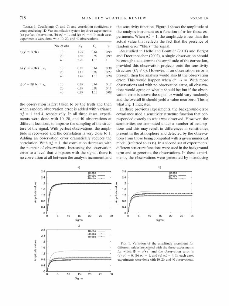
the sensitivity function. Figure 1 shows the amplitude of
the analysis increment as a function of s for these ex-
periments. When so2 5 1, the amplitude is less than the
actual value that reflects the fact that the presence of
random error ‘‘blurs’’ the signal.
As studied in Hello and Bouttier (2001) and Bergot
and Doerenbecher (2002), a single observation should
be enough to determine the amplitude of the correction,
provided this observation projects onto the sensitivity
structure (C1 6¼ 0). However, if an observation error is
present, then the analysis would also fit the observation
error. This would happen when s2 / ‘. With more
observations and with no observation error, all observa-
tions would agree on what a should be; but if the obser-
vation error is above the signal, a would vary randomly
and the overall fit should yield a value near zero. This is
what Fig. 1 indicates.
In those previous experiments, the background-error
covariance used a sensitivity structure function that cor-
responded exactly to what was observed. However, the
sensitivities are computed under a number of assump-
tions and this may result in differences in sensitivities
present in the atmosphere and detected by the observa-
tions from those being computed with a given numerical
model (referred to as vt). In a second set of experiments,
different structure functions were used in the background
term and to generate the observations. In these experi-
ments, the observations were generated by introducing
TABLE 1. Coefficients C1 and C2 and correlation coefficient r
computed using 1D-Var assimilation system for three experiments:
(a) perfect observation, (b) so2 5 1, and (c) so
2 5 4. In each case,
experiments were done with 10, 20, and 40 observations.
No. of obs C1 C2 r
a) y9 5 2(Hv) 10 1.29 0.64 0.99
20 1.96 0.97 0.99
40 2.26 1.13 1
b) y9 5 2(Hv) 1 eo 10 0.95 0.64 0.38
20 1.15 0.97 0.22
40 1.48 1.13 0.20
c) y9 5 2(Hv) 1 eo 10 0.89 0.64 0.17
20 0.89 0.97 0.11
40 0.87 1.13 0.08
FIG. 1. Variation of the amplitude increment for
different values associated with the three experiments
for which B 5 s2vvT and the observation error is
(a) so2 5 0, (b) so
2 5 1, and (c) so2 5 4. In each case,
experiments were done with 10, 20, and 40 observations.
718 M O N T H L Y W E A T H E R R E V I E W VOLUME 139
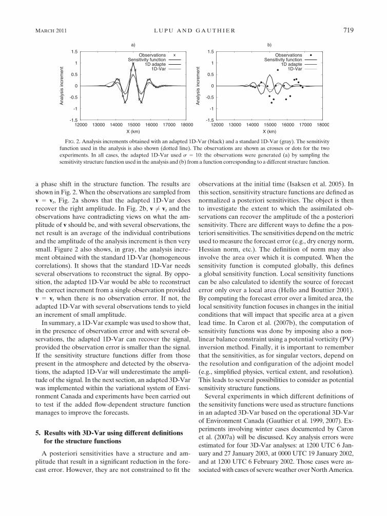
a phase shift in the structure function. The results are
shown in Fig. 2. When the observations are sampled from
v 5 vt, Fig. 2a shows that the adapted 1D-Var does
recover the right amplitude. In Fig. 2b, v 6¼ vt and the
observations have contradicting views on what the am-
plitude of v should be, and with several observations, the
net result is an average of the individual contributions
and the amplitude of the analysis increment is then very
small. Figure 2 also shows, in gray, the analysis incre-
ment obtained with the standard 1D-Var (homogeneous
correlations). It shows that the standard 1D-Var needs
several observations to reconstruct the signal. By oppo-
sition, the adapted 1D-Var would be able to reconstruct
the correct increment from a single observation provided
v 5 vt when there is no observation error. If not, the
adapted 1D-Var with several observations tends to yield
an increment of small amplitude.
In summary, a 1D-Var example was used to show that,
in the presence of observation error and with several ob-
servations, the adapted 1D-Var can recover the signal,
provided the observation error is smaller than the signal.
If the sensitivity structure functions differ from those
present in the atmosphere and detected by the observa-
tions, the adapted 1D-Var will underestimate the ampli-
tude of the signal. In the next section, an adapted 3D-Var
was implemented within the variational system of Envi-
ronment Canada and experiments have been carried out
to test if the added flow-dependent structure function
manages to improve the forecasts.
5. Results with 3D-Var using different definitionsfor the structure functions
A posteriori sensitivities have a structure and am-
plitude that result in a significant reduction in the fore-
cast error. However, they are not constrained to fit the
observations at the initial time (Isaksen et al. 2005). In
this section, sensitivity structure functions are defined as
normalized a posteriori sensitivities. The object is then
to investigate the extent to which the assimilated ob-
servations can recover the amplitude of the a posteriori
sensitivity. There are different ways to define the a pos-
teriori sensitivities. The sensitivities depend on the metric
used to measure the forecast error (e.g., dry energy norm,
Hessian norm, etc.). The definition of norm may also
involve the area over which it is computed. When the
sensitivity function is computed globally, this defines
a global sensitivity function. Local sensitivity functions
can be also calculated to identify the source of forecast
error only over a local area (Hello and Bouttier 2001).
By computing the forecast error over a limited area, the
local sensitivity function focuses in changes in the initial
conditions that will impact that specific area at a given
lead time. In Caron et al. (2007b), the computation of
sensitivity functions was done by imposing also a non-
linear balance constraint using a potential vorticity (PV)
inversion method. Finally, it is important to remember
that the sensitivities, as for singular vectors, depend on
the resolution and configuration of the adjoint model
(e.g., simplified physics, vertical extent, and resolution).
This leads to several possibilities to consider as potential
sensitivity structure functions.
Several experiments in which different definitions of
the sensitivity functions were used as structure functions
in an adapted 3D-Var based on the operational 3D-Var
of Environment Canada (Gauthier et al. 1999, 2007). Ex-
periments involving winter cases documented by Caron
et al. (2007a) will be discussed. Key analysis errors were
estimated for four 3D-Var analyses: at 1200 UTC 6 Jan-
uary and 27 January 2003, at 0000 UTC 19 January 2002,
and at 1200 UTC 6 February 2002. Those cases were as-
sociated with cases of severe weather over North America.
FIG. 2. Analysis increments obtained with an adapted 1D-Var (black) and a standard 1D-Var (gray). The sensitivity
function used in the analysis is also shown (dotted line). The observations are shown as crosses or dots for the two
experiments. In all cases, the adapted 1D-Var used s 5 10: the observations were generated (a) by sampling the
sensitivity structure function used in the analysis and (b) from a function corresponding to a different structure function.
MARCH 2011 L U P U A N D G A U T H I E R 719
For all cases, a posteriori sensitivities were computed
in different ways to minimize the 24-h forecast error as
measured with respect to a verifying analysis. The method
employed is explained in Laroche et al. (2002) and Caron
et al. (2007a). Four types of structure functions will be
considered in our study:
d a global sensitivity, for which the error is measured
globally,d a local sensitivity, for which the error is measured over
an area on the east coast of North America,d a hemispheric sensitivity function computed over the
latitudinal band 258–908N,d a sensitivity function, for which the control variable is
potential vorticity (PV), which constrains the sensitivity
to be more dynamically balanced, hereinafter called
PV-bal (Caron et al. 2007b).
All cases used the dry energy norm at initial and end
time. As already mentioned, the analysis increment (9)
has the direction of the sensitivity structure function and
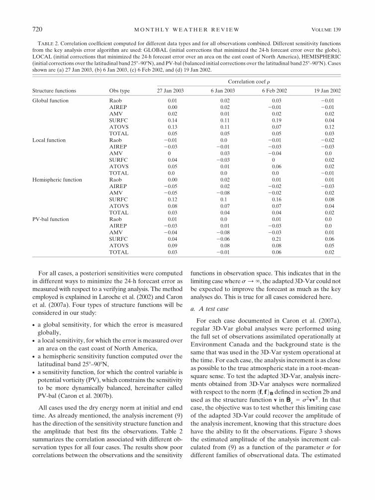
the amplitude that best fits the observations. Table 2
summarizes the correlation associated with different ob-
servation types for all four cases. The results show poor
correlations between the observations and the sensitivity
functions in observation space. This indicates that in the
limiting case where s / ‘, the adapted 3D-Var could not
be expected to improve the forecast as much as the key
analyses do. This is true for all cases considered here.
a. A test case
For each case documented in Caron et al. (2007a),
regular 3D-Var global analyses were performed using
the full set of observations assimilated operationally at
Environment Canada and the background state is the
same that was used in the 3D-Var system operational at
the time. For each case, the analysis increment is as close
as possible to the true atmospheric state in a root-mean-
square sense. To test the adapted 3D-Var, analysis incre-
ments obtained from 3D-Var analyses were normalized
with respect to the norm hf, f iB defined in section 2b and
used as the structure function v in ~Bx 5 s2vvT. In that
case, the objective was to test whether this limiting case
of the adapted 3D-Var could recover the amplitude of
the analysis increment, knowing that this structure does
have the ability to fit the observations. Figure 3 shows
the estimated amplitude of the analysis increment cal-
culated from (9) as a function of the parameter s for
different families of observational data. The estimated
TABLE 2. Correlation coefficient computed for different data types and for all observations combined. Different sensitivity functions
from the key analysis error algorithm are used: GLOBAL (initial corrections that minimized the 24-h forecast error over the globe),
LOCAL (initial corrections that minimized the 24-h forecast error over an area on the east coast of North America), HEMISPHERIC
(initial corrections over the latitudinal band 258–908N), and PV-bal (balanced initial corrections over the latitudinal band 258–908N). Cases
shown are (a) 27 Jan 2003, (b) 6 Jan 2003, (c) 6 Feb 2002, and (d) 19 Jan 2002.
Structure functions Obs type
Correlation coef r
27 Jan 2003 6 Jan 2003 6 Feb 2002 19 Jan 2002
Global function Raob 0.01 0.02 0.03 20.01
AIREP 0.00 0.02 20.01 20.01
AMV 0.02 0.01 0.02 0.02
SURFC 0.14 0.11 0.19 0.04
ATOVS 0.13 0.11 0.07 0.12
TOTAL 0.05 0.05 0.05 0.03
Local function Raob 20.01 0.0 20.01 20.02
AIREP 20.03 20.01 20.03 20.03
AMV 0 0.03 20.04 0.0
SURFC 0.04 20.03 0 0.02
ATOVS 0.05 0.01 0.06 0.02
TOTAL 0.0 0.0 0.0 20.01
Hemispheric function Raob 0.00 0.02 0.01 0.01
AIREP 20.05 0.02 20.02 20.03
AMV 20.05 20.08 20.02 0.02
SURFC 0.12 0.1 0.16 0.08
ATOVS 0.08 0.07 0.07 0.04
TOTAL 0.03 0.04 0.04 0.02
PV-bal function Raob 0.01 0.0 0.01 0.0
AIREP 20.03 0.01 20.03 0.0
AMV 20.04 20.08 20.03 0.01
SURFC 0.04 20.06 0.21 0.06
ATOVS 0.09 0.08 0.08 0.05
TOTAL 0.03 20.01 0.06 0.02
720 M O N T H L Y W E A T H E R R E V I E W VOLUME 139
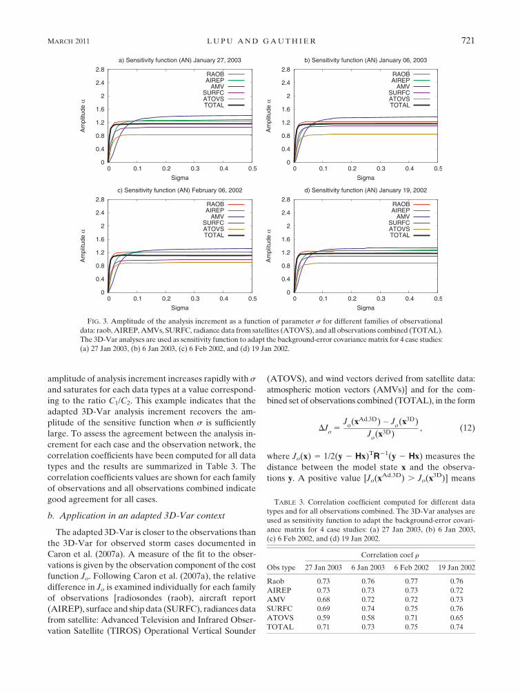
amplitude of analysis increment increases rapidly with s
and saturates for each data types at a value correspond-
ing to the ratio C1/C2. This example indicates that the
adapted 3D-Var analysis increment recovers the am-
plitude of the sensitive function when s is sufficiently
large. To assess the agreement between the analysis in-
crement for each case and the observation network, the
correlation coefficients have been computed for all data
types and the results are summarized in Table 3. The
correlation coefficients values are shown for each family
of observations and all observations combined indicate
good agreement for all cases.
b. Application in an adapted 3D-Var context
The adapted 3D-Var is closer to the observations than
the 3D-Var for observed storm cases documented in
Caron et al. (2007a). A measure of the fit to the obser-
vations is given by the observation component of the cost
function Jo. Following Caron et al. (2007a), the relative
difference in Jo is examined individually for each family
of observations [radiosondes (raob), aircraft report
(AIREP), surface and ship data (SURFC), radiances data
from satellite: Advanced Television and Infrared Obser-
vation Satellite (TIROS) Operational Vertical Sounder
(ATOVS), and wind vectors derived from satellite data:
atmospheric motion vectors (AMVs)] and for the com-
bined set of observations combined (TOTAL), in the form
DJo
5J
o(xAd.3D)� J
o(x3D)
Jo(x3D)
, (12)
where Jo(x) 5 1/2(y 2 Hx)TR21(y 2 Hx) measures the
distance between the model state x and the observa-
tions y. A positive value [Jo(xAd.3D) . Jo(x3D)] means
TABLE 3. Correlation coefficient computed for different data
types and for all observations combined. The 3D-Var analyses are
used as sensitivity function to adapt the background-error covari-
ance matrix for 4 case studies: (a) 27 Jan 2003, (b) 6 Jan 2003,
(c) 6 Feb 2002, and (d) 19 Jan 2002.
Obs type
Correlation coef r
27 Jan 2003 6 Jan 2003 6 Feb 2002 19 Jan 2002
Raob 0.73 0.76 0.77 0.76
AIREP 0.73 0.73 0.73 0.72
AMV 0.68 0.72 0.72 0.73
SURFC 0.69 0.74 0.75 0.76
ATOVS 0.59 0.58 0.71 0.65
TOTAL 0.71 0.73 0.75 0.74
FIG. 3. Amplitude of the analysis increment as a function of parameter s for different families of observational
data: raob, AIREP, AMVs, SURFC, radiance data from satellites (ATOVS), and all observations combined (TOTAL).
The 3D-Var analyses are used as sensitivity function to adapt the background-error covariance matrix for 4 case studies:
(a) 27 Jan 2003, (b) 6 Jan 2003, (c) 6 Feb 2002, and (d) 19 Jan 2002.
MARCH 2011 L U P U A N D G A U T H I E R 721
that that the adapted 3D-Var analyses are farther away
from the observations than the corresponding operational
analysis and, conversely, a negative value [Jo(xAd.3D) ,
Jo(x3D)] means that the adapted 3D-Var analyses fit the
observations better than 3D-Var.
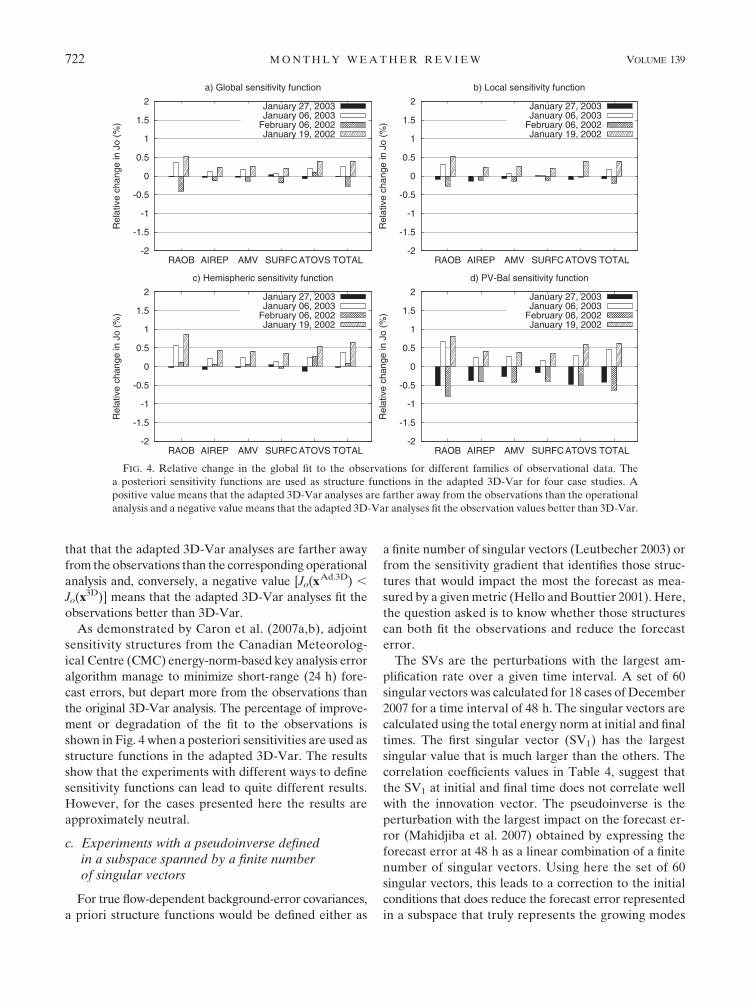
As demonstrated by Caron et al. (2007a,b), adjoint
sensitivity structures from the Canadian Meteorolog-
ical Centre (CMC) energy-norm-based key analysis error
algorithm manage to minimize short-range (24 h) fore-
cast errors, but depart more from the observations than
the original 3D-Var analysis. The percentage of improve-
ment or degradation of the fit to the observations is
shown in Fig. 4 when a posteriori sensitivities are used as
structure functions in the adapted 3D-Var. The results
show that the experiments with different ways to define
sensitivity functions can lead to quite different results.
However, for the cases presented here the results are
approximately neutral.
c. Experiments with a pseudoinverse definedin a subspace spanned by a finite numberof singular vectors
For true flow-dependent background-error covariances,
a priori structure functions would be defined either as
a finite number of singular vectors (Leutbecher 2003) or
from the sensitivity gradient that identifies those struc-
tures that would impact the most the forecast as mea-
sured by a given metric (Hello and Bouttier 2001). Here,
the question asked is to know whether those structures
can both fit the observations and reduce the forecast
error.
The SVs are the perturbations with the largest am-
plification rate over a given time interval. A set of 60
singular vectors was calculated for 18 cases of December
2007 for a time interval of 48 h. The singular vectors are
calculated using the total energy norm at initial and final
times. The first singular vector (SV1) has the largest
singular value that is much larger than the others. The
correlation coefficients values in Table 4, suggest that
the SV1 at initial and final time does not correlate well
with the innovation vector. The pseudoinverse is the
perturbation with the largest impact on the forecast er-
ror (Mahidjiba et al. 2007) obtained by expressing the
forecast error at 48 h as a linear combination of a finite
number of singular vectors. Using here the set of 60
singular vectors, this leads to a correction to the initial
conditions that does reduce the forecast error represented
in a subspace that truly represents the growing modes
FIG. 4. Relative change in the global fit to the observations for different families of observational data. The
a posteriori sensitivity functions are used as structure functions in the adapted 3D-Var for four case studies. A
positive value means that the adapted 3D-Var analyses are farther away from the observations than the operational
analysis and a negative value means that the adapted 3D-Var analyses fit the observation values better than 3D-Var.
722 M O N T H L Y W E A T H E R R E V I E W VOLUME 139
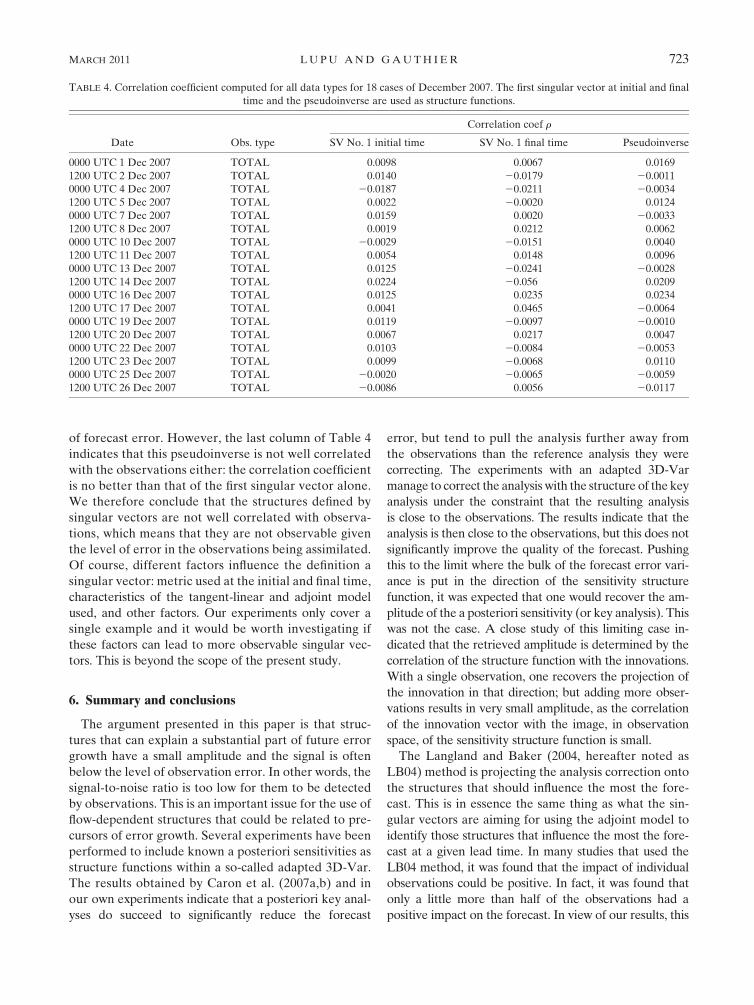
of forecast error. However, the last column of Table 4
indicates that this pseudoinverse is not well correlated
with the observations either: the correlation coefficient
is no better than that of the first singular vector alone.
We therefore conclude that the structures defined by
singular vectors are not well correlated with observa-
tions, which means that they are not observable given
the level of error in the observations being assimilated.
Of course, different factors influence the definition a
singular vector: metric used at the initial and final time,
characteristics of the tangent-linear and adjoint model
used, and other factors. Our experiments only cover a
single example and it would be worth investigating if
these factors can lead to more observable singular vec-
tors. This is beyond the scope of the present study.
6. Summary and conclusions
The argument presented in this paper is that struc-
tures that can explain a substantial part of future error
growth have a small amplitude and the signal is often
below the level of observation error. In other words, the
signal-to-noise ratio is too low for them to be detected
by observations. This is an important issue for the use of
flow-dependent structures that could be related to pre-
cursors of error growth. Several experiments have been
performed to include known a posteriori sensitivities as
structure functions within a so-called adapted 3D-Var.
The results obtained by Caron et al. (2007a,b) and in
our own experiments indicate that a posteriori key anal-
yses do succeed to significantly reduce the forecast
error, but tend to pull the analysis further away from
the observations than the reference analysis they were
correcting. The experiments with an adapted 3D-Var
manage to correct the analysis with the structure of the key
analysis under the constraint that the resulting analysis
is close to the observations. The results indicate that the
analysis is then close to the observations, but this does not
significantly improve the quality of the forecast. Pushing
this to the limit where the bulk of the forecast error vari-
ance is put in the direction of the sensitivity structure
function, it was expected that one would recover the am-
plitude of the a posteriori sensitivity (or key analysis). This
was not the case. A close study of this limiting case in-
dicated that the retrieved amplitude is determined by the
correlation of the structure function with the innovations.
With a single observation, one recovers the projection of
the innovation in that direction; but adding more obser-
vations results in very small amplitude, as the correlation
of the innovation vector with the image, in observation
space, of the sensitivity structure function is small.
The Langland and Baker (2004, hereafter noted as
LB04) method is projecting the analysis correction onto
the structures that should influence the most the fore-
cast. This is in essence the same thing as what the sin-
gular vectors are aiming for using the adjoint model to
identify those structures that influence the most the fore-
cast at a given lead time. In many studies that used the
LB04 method, it was found that the impact of individual
observations could be positive. In fact, it was found that
only a little more than half of the observations had a
positive impact on the forecast. In view of our results, this
TABLE 4. Correlation coefficient computed for all data types for 18 cases of December 2007. The first singular vector at initial and final
time and the pseudoinverse are used as structure functions.
Date Obs. type
Correlation coef r
SV No. 1 initial time SV No. 1 final time Pseudoinverse
0000 UTC 1 Dec 2007 TOTAL 0.0098 0.0067 0.0169
1200 UTC 2 Dec 2007 TOTAL 0.0140 20.0179 20.0011
0000 UTC 4 Dec 2007 TOTAL 20.0187 20.0211 20.0034
1200 UTC 5 Dec 2007 TOTAL 0.0022 20.0020 0.0124
0000 UTC 7 Dec 2007 TOTAL 0.0159 0.0020 20.0033
1200 UTC 8 Dec 2007 TOTAL 0.0019 0.0212 0.0062
0000 UTC 10 Dec 2007 TOTAL 20.0029 20.0151 0.0040
1200 UTC 11 Dec 2007 TOTAL 0.0054 0.0148 0.0096
0000 UTC 13 Dec 2007 TOTAL 0.0125 20.0241 20.0028
1200 UTC 14 Dec 2007 TOTAL 0.0224 20.056 0.0209
0000 UTC 16 Dec 2007 TOTAL 0.0125 0.0235 0.0234
1200 UTC 17 Dec 2007 TOTAL 0.0041 0.0465 20.0064
0000 UTC 19 Dec 2007 TOTAL 0.0119 20.0097 20.0010
1200 UTC 20 Dec 2007 TOTAL 0.0067 0.0217 0.0047
0000 UTC 22 Dec 2007 TOTAL 0.0103 20.0084 20.0053
1200 UTC 23 Dec 2007 TOTAL 0.0099 20.0068 0.0110
0000 UTC 25 Dec 2007 TOTAL 20.0020 20.0065 20.0059
1200 UTC 26 Dec 2007 TOTAL 20.0086 0.0056 20.0117
MARCH 2011 L U P U A N D G A U T H I E R 723
seems to indicate that the signal is at the noise level and
can barely be detected by the available observations.
These results are important and more thought is
needed on how to include information about precursors
in the analysis. An element that needs to be considered
is that the analysis may have to wait for the instability
to develop above the signal-to-noise ratio for the ob-
servations to be able to detect it and properly correct the
initial conditions. In a sense, this would indicate that
evolved covariances obtained from a Kalman filter as
obtained from an ensemble Kalman filter (Houtekamer
et al. 2009) should be better observable than covariances
represented in a subspace spanned by singular vectors.
However, evolved singular vectors could be a good
prospect. This will be the object of future work.
Acknowledgments. Authors would like to deeply thank
Dr. Jean-Francxois Caron who provided the a posteriori
sensitivity functions used in this study. Stimulating dis-
cussions with Drs. Mark Buehner and Ahmed Mahidjiba
were very helpful during the course of this study. They
kindly provided the singular vectors and the pseudoinverses
used in this study. Environment Canada provided the
computing facilities, and technical assistance for the use
of their assimilation system.
This work has been funded mostly by Grant 500-B of
the Canadian Foundation for Climate and Atmospheric
Sciences (CFCAS) for the project on the Impact of Ob-
serving Systems on Forecasting Extreme Weather in the
Short, Medium and Extended Range: A Canadian Con-
tribution to THORPEX, with additional support from
Discovery Grant 357091 of the Natural Sciences and
Engineering Research Council (NSERC) of Canada.
APPENDIX
Formulation of the Adapted 3D-Var
Adding a sensitive component to Bh led to
~Bx
5 Bh
1 s2vvT,
where hv, viB [ vTBh21v 5 1. Using the Sherman–
Morrison formula (Golub and Van Loan 1996), the in-
verse of ~Bx is found to be
~B�1x 5 B�1/2T
h I� s2
(s2 1 1)(B�1/2
h v)(B�1/2h v)T
� �B�1/2
h
(A1)
and the 3D-Var cost function (1) can be rewritten as
J(dx) 51
2dxTB�1/2T
h I� s2
(s2 1 1)(B�1/2
h v)(B�1/2h v)T
� �
3 B�1/2h dx 1
1
2(Hdx� y9)TR�1(Hdx� y9).
Defining the change of variables, j 5 Bh21/2dx and
~v 5 B�1/2h v yields
J(j) 51
2jT I� s2
s2 1 1~v~vT
� �j 1
1
2(HB1/2
h j � y9)T
3 R�1(HB1/2h j � y9) 5 J
b(j) 1 J
o(j). (A2)
So defined, the sensitivity structure function is such
that
~vT~v 5 vTB�1/2h B�1/2
h v 5 vTB�1h v 5 1.
In terms of these new variables, we have
I� s2
s2 1 1~v~vT
� �5 I 1
(ffiffiffiffiffiffiffiffiffiffiffiffiffis2 1 1p
� s2 � 1)
s2 1 1~v~vT
� �25 LTL,
with
L 5 I 1
ffiffiffiffiffiffiffiffiffiffiffiffiffis2 1 1p
� s2 � 1
s2 1 1
� �~v~vT 5 LT. (A3)
This allows us to introduce another change of variable
j 5 Lj, so that j 5 L�1~j. The inverse of L is found to be
L�1 5 I 1 (ffiffiffiffiffiffiffiffiffiffiffiffiffis2 1 1p
� 1)~v~vT,
so that (A2) is finally expressed as
J(~j) 51
2~j
T~j 11
2(HB1/2
h L�1~j � y9)TR�1(HB1/2h L�1~j � y9).
(A4)
Its gradient is readily found to be
$~jJ 5 ~j 1 L�TB1/2
h HTR�1(HB1/2h L�1~j � y9).
REFERENCES
Beck, A., and M. Ehrendorfer, 2005: Singular-vector-based co-
variance propagation in a quasigeostrophic assimilation sys-
tem. Mon. Wea. Rev., 133, 1295–1310.
Bergot, T., and A. Doerenbecher, 2002: A study on the optimiza-
tion of the deployment of targeted observations using adjoint-
based methods. Quart. J. Roy. Meteor. Soc., 128, 1689–1712.
Berre, L., G. Desroziers, L. Raynaud, R. Montroty, and F. Gibier,
2009: Consistent operational ensemble variational assimila-
tion. Proc. CAWCR Workshop on Ensemble Prediction and
724 M O N T H L Y W E A T H E R R E V I E W VOLUME 139
Data Assimilation, Melbourne, Australia, Australian Bureau
of Meteorology, Paper 196, 8 pp.
Buehner, M., P. L. Houtekamer, C. Charette, H. L. Mitchell, and
B. He, 2010a: Intercomparaison of variational data assimila-
tion and ensemble Kalman filter for global deterministic NWP.
Part I: Description and single-observation experiments. Mon.
Wea. Rev., 138, 1550–1566.
——, ——, ——, ——, and ——, 2010b: Intercomparaison of var-
iational data assimilation and ensemble Kalman filter for global
deterministic NWP. Part II: One-month experiments with real
observations. Mon. Wea. Rev., 138, 1567–1586.
Buizza, R., J.-R. Bidlot, N. Wedi, M. Fuentes, M. Hamrud, G. Holt,
and F. Vitart, 2007a: The new ECMWF VAREPS (Variable
Resolution Ensemble Prediction System). Quart. J. Roy. Me-
teor. Soc., 133, 681–695.
——, C. Cardinali, G. Kelly, and J.-N. Thepaut, 2007b: The value of
observations. II: The value of observations located in singular-
vector-based target areas. Quart. J. Roy. Meteor. Soc., 133,
1817–1832.
Cardinali, C., R. Buizza, G. Kelly, M. Shapiro, and J.-N. Thepaut,
2007: The value of observations. III: Influence of weather
regimes on targeting. Quart. J. Roy. Meteor. Soc., 133, 1833–
1842.
Caron, J.-F., M. K. Yau, S. Laroche, and P. Zwack, 2007a: The
characteristics of key analysis errors. Part I: Dynamical bal-
ance and comparison with observations. Mon. Wea. Rev., 135,249–266.
——, ——, ——, and ——, 2007b: The characteristics of key
analysis errors. Part II: The importance of the PV corrections
and the impact of balance. Mon. Wea. Rev., 135, 267–280.
Evensen, G., 1994: Sequencial data assimilation with a nonlinear
quasi-geostrophic model using Monte Carlo methods to fore-
cast error statistics. J. Geophys. Res., 99, 10 143–10 162.
Fisher, M., 1998: Development of a simplified Kalman Filter.
ECMWF Research Department Tech. Memo. 260, ECMWF,
16 pp.
——, and E. Andersson, 2001: Developments in 4D-Var and
Kalman filtering. ECMWF Research Department Tech. Memo.
347, ECMWF, 36 pp.
Gauthier, P., C. Charette, L. Fillion, P. Koclas, and S. Laroche,
1999: Implementation of a 3D variational data assimilation
system at the Canadian Meteorological Centre. Part I: The
global analysis. Atmos.–Ocean, 37, 103–156.
——, M. Tanguay, S. Laroche, S. Pellerin, and J. Morneau, 2007:
Extension of 3DVAR to 4DVAR: Implementation of 4DVAR
at the Meteorological Service of Canada. Mon. Wea. Rev., 135,
2339–2354.
Golub, H. G., and C. F. Van Loan, 1996: Matrix Computations. 3rd
ed. The John Hopkins University Press, 694 pp.
Hamill, T., and C. Snyder, 2000: A hybrid ensemble Kalman filter–
3D variational analysis scheme. Mon. Wea. Rev., 128, 2905–
2919.
Hello, G., and F. Bouttier, 2001: Using adjoint sensitivity as a local
structure function in variational data assimilation. Nonlinear
Processes Geophys., 8, 347–355.
——, F. Lalaurette, and J.-N. Thepaut, 2000: Combined use of
sensitivity information and observations to improve meteo-
rological forecasts: A feasibility study applied to the ‘Christ-
mas storm’ case. Quart. J. Roy. Meteor. Soc., 126, 621–647.
Houtekamer, P. L., H. L. Mitchell, and X. Deng, 2009: Model error
representation in an operational ensemble Kalman filter.
Mon. Wea. Rev, 137, 2126–2143.
Isaksen, L., M. Fisher, E. Andersson, and J. Barkmeijer, 2005: The
structure and realism of sensitivity perturbations and their
interpretation as ‘‘Key analysis errors.’’ Quart. J. Roy. Meteor.
Soc., 131, 3053–3078.
Joly, A., and Coauthors, 1999: Overview of the field phase of the
Fronts and Atlantic Storm Track Experiment (FASTEX)
project. Quart. J. Roy. Meteor. Soc., 125, 3131–3164.
Kelly, G., J.-N. Thepaut, R. Buizza, and C. Cardinali, 2007: The value
of observations. I: Data denial experiments for the Atlantic and
the Pacific. Quart. J. Roy. Meteor. Soc., 133, 1803–1815.
Klinker, E., F. Rabier, and R. Gelaro, 1998: Estimation of key
analysis errors using the adjoint technique. Quart. J. Roy.
Meteor. Soc., 124, 1909–1933.
Lacarra, J. F., and O. Talagrand, 1988: Short-range evolution of
small perturbations in a barotropic model. Tellus, 40A, 81–95.
Langland, R. H., 2005a: Observation impact during the North
Atlantic TreC-2003. Mon. Wea. Rev., 133, 2297–2309.
——, 2005b: Issues in targeted observing. Quart. J. Roy. Meteor.
Soc., 131, 3409–3425.
——, and N. L. Baker, 2004: Estimation of observation impact
using the NRL variational data assimilation adjoint system.
Tellus, 56A, 189–201.
——, and Coauthors, 1999: The North Pacific Experiment
(NORPEX-98): Targeted observations for improved North
American weather forecasts. Bull. Amer. Meteor. Soc., 80,
1363–1384.
——, M. A. Shapiro, and R. Gelaro, 2002: Initial condition sensi-
tivity and error growth in forecasts of the 25 January 2000 East
Coast snowstorm. Mon. Wea. Rev., 130, 957–974.
Laroche, S., M. Tanguay, A. Zadra, and J. Morneau, 2002: Use of
adjoint sensitivity analysis to diagnose the CMC Global anal-
ysis performance: A case study. Atmos.–Ocean, 40 (4), 423–443.
Leutbecher, M., 2003: A reduced rank estimate of forecast error
variance changes due to intermittent modifications of the ob-
serving network. J. Atmos. Sci., 60, 729–742.
Liu, Z. Q., and F. Rabier, 2002: The interaction between model
resolution, observation resolution and observation density in
data assimilation: A one-dimensional study. Quart. J. Roy.
Meteor. Soc., 128, 1367–1386.
Mahidjiba, A., M. Buehner, and A. Zadra, 2007: Excitation of
Rossby-wave trains: Optimal growth of forecast errors. Me-
teor. Z., 16, 665–673.
Molteni, F., R. Buizza, T. N. Palmer, and T. Petroliagis, 1996: The
ECMWF ensemble prediction system: Methodology and val-
idation. Quart. J. Roy. Meteor. Soc., 122, 73–120.
Petersen, G. N., and A. J. Thorpe, 2007: The impact on weather
forecasts of targeted observations during A-TreC. Quart. J. Roy.
Meteor. Soc., 133, 417–431.
MARCH 2011 L U P U A N D G A U T H I E R 725