SIAM J. CONTROL Vol. 10, No. 2, May 1972 CONTROLLABILITY, OBSERVABILITY AND OPTIMAL FEEDBACK CONTROL OF AFFINE HEREDITARY DIFFERENTIAL SYSTEMS* M. C. DELFOUR]" AND S. K. MITTER:I: Abstract. This paper is concerned with two aspects of the control of affine hereditary differential systems. They are (i) the theory of various types of controllability and observability for such systems and (ii) the problem of optimal feedback control with a quadratic cost. The study is undertaken within the framework of hereditary differential systems with initial data in the space M (cf. Delfour and Mitter [6], [7]). The main result of this paper is the existence and characterization of the optimal feedback operator for the system. 1. Introduction. Perhaps the most useful part of optimal control theory for ordinary differential equations is the theory of optimal control of linear differential systems with a quadratic cost criterion. This theory is also the most complete, both for systems evolving in a finite-time interval as well as over an infinite-time interval. It is well known that in the finite-time case the optimal control can be expressed in linear feedback form, where the "feedback gains" satisfy a matrix differential equation of Riccati type. In the infinite-time case by using the theory of con- trollability and observability, the asymptotic behavior of the controlled system can be studied and a rather complete solution to the problem is available. The present paper is concerned with (i) generalization of the theory of con- trollability and observability to affine hereditary differential systems and (ii) a study of the optimal feedback control problem for affine hereditary differential systems with a quadratic cost. The theory is currently being completed in order to show the relation of the theory of controllability and observability to the infinite-time quadratic cost problem. The optimal control problem studied in this paper was first formulated and studied by Krasovskii 233, [24] using the space of continuous functions as the space of initial data and using dynamic programming arguments. This problem has also been studied by Ross and Fltigge-Lotz [303, Eller, Aggarwal and Banks 13], Kushner and Barnea [25] and Alekal, Brunovsky, Chyung and Lee [1], in each case using Carath6odory-Hamilton-Jacobi type arguments. The basic disadvantage of the method used by these authors is that it necessitates a direct study of a complicated set of coupled ordinary and first order partial differential equations before the existence of a feedback control can be asserted. In Delfour and Mitter I6], [7] we have developed a theory of hereditary differential systems where the initial datum is chosen to lie in the space * Received by the editors September 13, 1971, and in revised form January 21, 1972. Presented at the NSF Regional Conference on Control Theory, held at the University of Maryland Baltimore County, August 23-27, 1971. 5- Centre de Recherches Math6matiques, Universit6 de Montr6al, Montr6al 101, Qu6bec, Canada. Electronic Systems Laboratory and Electrical Engineering Department, Massachusetts Institute of Technology, Cambridge, Massachusetts 02139. The work of this author was supported in part by the National Science Foundation under Grant GK-25781 and by the Air Force Office of Scientific Research under Grant AFOSR-70-1941. 298

Welcome message from author
This document is posted to help you gain knowledge. Please leave a comment to let me know what you think about it! Share it to your friends and learn new things together.
Transcript

SIAM J. CONTROLVol. 10, No. 2, May 1972
CONTROLLABILITY, OBSERVABILITY ANDOPTIMAL FEEDBACK CONTROL OF
AFFINE HEREDITARY DIFFERENTIAL SYSTEMS*
M. C. DELFOUR]" AND S. K. MITTER:I:
Abstract. This paper is concerned with two aspects of the control of affine hereditary differentialsystems. They are (i) the theory of various types of controllability and observability for such systemsand (ii) the problem of optimal feedback control with a quadratic cost. The study is undertaken withinthe framework of hereditary differential systems with initial data in the space M (cf. Delfour andMitter [6], [7]). The main result of this paper is the existence and characterization of the optimalfeedback operator for the system.
1. Introduction. Perhaps the most useful part of optimal control theory forordinary differential equations is the theory of optimal control of linear differentialsystems with a quadratic cost criterion. This theory is also the most complete, bothfor systems evolving in a finite-time interval as well as over an infinite-time interval.It is well known that in the finite-time case the optimal control can be expressed inlinear feedback form, where the "feedback gains" satisfy a matrix differentialequation of Riccati type. In the infinite-time case by using the theory of con-trollability and observability, the asymptotic behavior of the controlled systemcan be studied and a rather complete solution to the problem is available.
The present paper is concerned with (i) generalization of the theory of con-trollability and observability to affine hereditary differential systems and (ii) astudy of the optimal feedback control problem for affine hereditary differentialsystems with a quadratic cost. The theory is currently being completed in orderto show the relation of the theory of controllability and observability to theinfinite-time quadratic cost problem.
The optimal control problem studied in this paper was first formulated andstudied by Krasovskii 233, [24] using the space of continuous functions as thespace of initial data and using dynamic programming arguments. This problemhas also been studied by Ross and Fltigge-Lotz [303, Eller, Aggarwal and Banks13], Kushner and Barnea [25] and Alekal, Brunovsky, Chyung and Lee [1], ineach case using Carath6odory-Hamilton-Jacobi type arguments. The basicdisadvantage of the method used by these authors is that it necessitates a directstudy of a complicated set of coupled ordinary and first order partial differentialequations before the existence of a feedback control can be asserted.
In Delfour and Mitter I6], [7] we have developed a theory of hereditarydifferential systems where the initial datum is chosen to lie in the space
* Received by the editors September 13, 1971, and in revised form January 21, 1972. Presentedat the NSF Regional Conference on Control Theory, held at the University of Maryland BaltimoreCounty, August 23-27, 1971.
5- Centre de Recherches Math6matiques, Universit6 de Montr6al, Montr6al 101, Qu6bec, Canada.Electronic Systems Laboratory and Electrical Engineering Department, Massachusetts Institute
of Technology, Cambridge, Massachusetts 02139. The work of this author was supported in partby the National Science Foundation under Grant GK-25781 and by the Air Force Office of ScientificResearch under Grant AFOSR-70-1941.
298
AFFINE HEREDITARY DIFFERENTIAL SYSTEMS 299
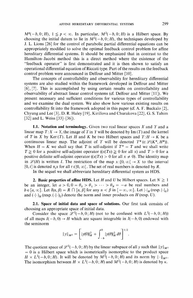
MP(-b, 0; H), 1 __< p < . In particular, M2(-b, 0; H) is a Hilbert space. Bychoosing the initial datum to lie in M2(-b, 0; H), the techniques developed byJ. L. Lions [26] for the control of parabolic partial differential equations can beappropriately modified to solve the optimal feedback control problem for affinehereditary differential systems. It should be emphasized that in contrast to theHamilton-Jacobi method this is a direct method where the existence of the"feedback operator" is first demonstrated and it is then shown to satisfy anoperational differential equation of Riccati type. Part of the results on the feedbackcontrol problem were announced in Delfour and Mitter [103.
The concepts of controllability and observability for hereditary differentialsystems are also studied within the framework developed in Delfour and Mitter[63, [7]. This is accomplished by using certain results on controllability andobservability of abstract linear control systems (cf. Delfour and Mitter [11]). Wepresent necessary and sufficient conditions for various types of controllabilityand we examine the dual system. We also show how various existing results oncontrollability fit into the framework adopted in this paper (cf. A. F. Buckalo [2],Chyung and Lee [33, D. R. Haley [193, Kirillova and Churakova [223, G. S. Tahim[32] and L. Weiss [33]-[363).
1.1. Notation and terminology. Given two real linear spaces X and Y and alinear map T’X Y, the image of T in Y will be denoted by Im (T) and the kernelof T in X by Ker (T). Let H and K be two Hilbert spaces and T’H K be acontinuous linear map. The adjoint of T will be denoted T* ( 5P(K*,H*)).When H K we shall say that T is self-adjoint if T* T and we shall writeT __> 0 for a positive self-adjoint operator ((x] Tx) >= 0 for all x) and T > 0 for apositive definite self-adjoint operator ((x] Tx) > 0 for all x 4: 0). The identity mapin (H) is written I. The restriction of the map x’[0, X to the interval[0, t] is denoted ntx for all ]0, [. The set of real numbers is denoted by R.
In the sequel we shall abbreviate hereditary differential system as HDS.
2. Basic properties of ailine HDS. Let H and U be Hilbert spaces. Let N >__be an integer, let a > 0,0 0o > 01 >... > 0N -a be real numbers andb Ia, ]. Let I(, fl) g I, fl] for any < fl in [-, ]. Let I’ln (resp. I’lu)and (. I’)n (resp. (. I’)v) denote the norm and inner products on H (resp. U).
2.1. Space of initial data and space of solutions. Our first task consists ofchoosing an appropriate space of initial data.
Consider the space 2(-b, 0; H) (not to be confused with L2(-b, 0; H))of all maps I(-b, 0) l H which are square integrable in I(-b, 0) endowed withthe seminorm
yll--ly(0)l + ly(O)ldO
The quotient space of 2(_ b, 0 H) by the linear subspace of all y such that y t2
0 is a Hilbert space which is isometrically isomorphic to the product spaceH LZ(-b, 0; H). It will be denoted by MZ(-b, 0; H) and its norm by ]].The isomorphism between H L2( b, 0;H) and M2( b, 0;H) is denoted by

300 M.C. DELFOUR AND S. K. MITTER
In order to discuss the Cauchy problem we must also describe the space inwhich solutions will be sought. Let 1 =< p < , o R. For all ]to, [ we denoteby ACP(to, t; H) the vector space of all absolutely continuous maps [to, t] Hwith a derivative in LP(to, t;H). When ACP(to, t;H) is endowed with the norm
x c X(to)l,+ Ts(s) s
it is a Banach space isometrically isomorphic to H LP(to, t;H). In particular,AC2(to, t; H) is a Hilbert space. We shall also need C(to, t;H), the Banach spaceof all continuous maps [to, t] - H endowed with the sup norm c.
When we consider the evolution of a system in an infinite-time interval it isuseful and quite natural to introduce the following spaces. Let nt(x be the re-striction of the map x" [to, [ - H to the interval [to, t], ]to, v[. Denote byLioc(to, ;H), ACoc(to, ;H) and Clo(to, ;H) the vector space of all mapsx’[to, - H such that for all ]to, , nt(x) is in LP(to, t; H), ACP(to, t; H)and C(to, t;H), respectively. They are Fr6chet spaces (cf. Delfour 5]) when theirrespective topologies are defined by the saturated family of seminorms qt(x)
n(x) F, 6 ]to, , where F is either Lp, ACp or C.
2.2. System description. Consider the affine hereditary differential system ’defined on [0, "dx n fx(t4- Oi),t 4- OiO0t--(/7)-- Aoo(t).x(t q- i--1 Ai(t)h(t + Oi), + 0 <
(2.1) 4- yo-b
Aol(t, O)(h(t + 0), + 0 <
+ B(t)v(t) + f(t) a.e. in [0, ),
x(0) h(0), h e M2(-b, 0;H),
where Aoo and A (i 1, 2, ..., N) are in Llc(0, o (H)), Aol Llc(0,-b, 0; 5(H)), B e Llo(0, oe ;(U, H)), v e L12o(0, oe U) and fe L12o(0, oe ;H).
v is to be thought of as the control to be applied to the system and f is a knownexternal input to the system. Under the above hypotheses, (2.1) has a unique solu-tion 4(" ;h, v) in AC2o(O, oe ;H) and the map
(2.2) (h, v) 4)(. ;h, v)’M2( b, 0;H) x Lo(0, o;U) - ACo(O o ;H)
is affine and continuous (cf. Delfour and Mitter [6], [7] and Delfour [5]). We alsohave the variation of constants formula
(2.3) b(t; h, v) O(t, O)h + (t, s)B(s)v(s) ds + (t, s)f(s) ds,
where
O
(t, s)h d(t, s)h(O) + (t, s, a)h(a) da,-b
AFFINE HEREDITARY DIFFERENTIAL SYSTEMS 301
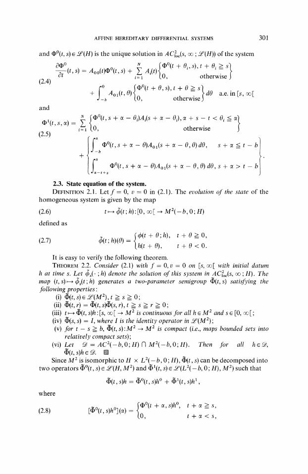
and O(t, s) e 5(’(H) is the unique solution in AC(oc(S, (H)) of the system
(2.4)
and
--xN (t + Oi’s)’t + Oi stt(t s)= Aoo(t)((t, s) + Ai(tt i-- (0, otherwiseo a)(t + o ) + o > }+ Aol(t,0) dO a.e. in[s, [-b (0, otherwise
u (o(t ,s +- Oi)Ai(s + - Oi), + s- < 0 <3dOx(t, s, a) ,
i= (0, otherwise(2.5)
(t, s + O)Aol(S + O, O)dO, s + <= b-b
+(t,s + O)Ao(S + - O,O) dO, s + > t- b
--t+s
2.3. State equation of the system.DEFINITION 2.1. Let f 0, v 0 in (2.1). The evolution of the state of the
homogeneous system is given by the map
(2.6) ((t; h)" [0, [ M2( b, 0; H)
defined as
+ 0;h), + 0 0,(2.7) q(t;h)(0)=
h(t + O), + O < O.
It is easy to verify the following theorem.THEOREM 2.2. Consider (2.1) with f O, v 0 on Is, [ with initial datum
h at time s. Let s(" ;h) denote the solution of this system in ACoc(S, o ;H). Themap (t,s)-- )s(t; h) generates a two-parameter semigroup (t,s) satisfying thefollowing properties"
(i) (b(t, s) (M2), => s _>_ 0;(ii) O(t, r) O(t, s)O(s, r), >_ s >= r >= 0;
(iii) t- (t, s)h’[s, [ - M2 is continuous for all h e M2 and s e [0, [;(iv) (s, s) I, where I is the identity operator in 5(M2);(v) for s >= b, (t, s)’M2 M2 is compact (i.e., maps bounded sets into
relatively compact sets);(vi) Let @ AC2(-b, O; H) VIM2(-b,0;H). Then for all beg,
O(t, s)h e .Since M2 is isomorphic to H L2(- b, 0; H), ((t, s) can be decomposed into
two operators (t, s) e &a(H, M2) and (t, s) 9(L2(- b, 0; H), M2) such that
where
(2.8)
(t, s)h (t, s)h + (t, s)h
@(t + , s)h,[(t’s)h](a)
(0,
t+a>s,
t+<s,
302 M. C. DELFOUR AND S. K. MITTER
and
(2.9) fo (t + , s, ,)h(,) d,[I1(t, s)hX](z)h-(t + - s),
t+e>s,
t+cz<s.
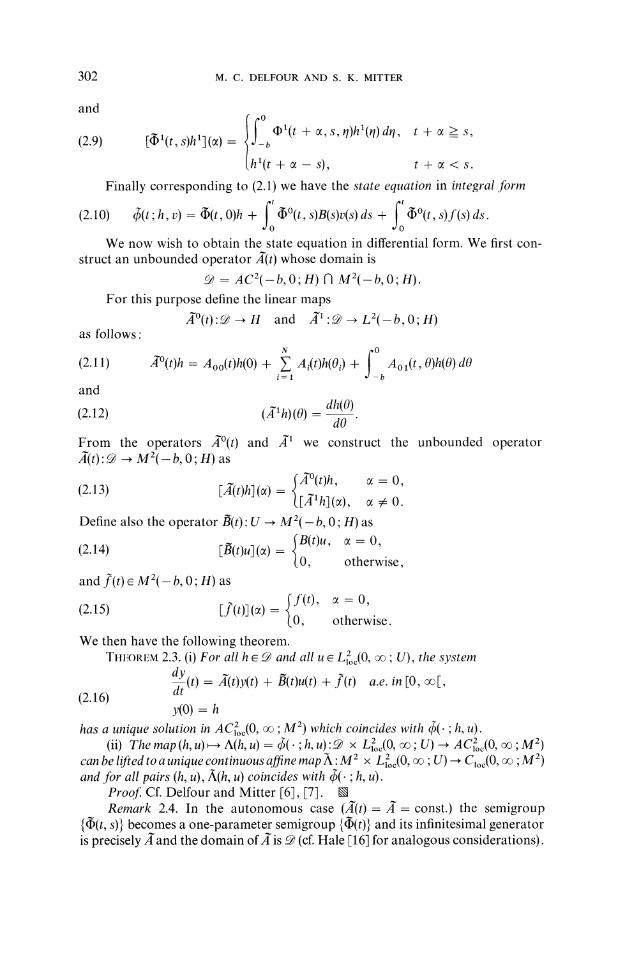
Finally corresponding to (2.1) we have the state equation in integral form
(2.10) (t;h, v) (t, O)h + (t, s)B(s)v(s)ds + (t, s)f(s)ds.
We now wish to obtain the state equation in differential form. We first con-struct an unbounded operator A(t) whose domain is
AC2(-b,O;H) fl M2(-b,O; H).For this purpose define the linear maps
(t)’6 --, U and ’- L2(-b,O;H)as follows"
(2.11)
and
(2.12)
N fo(t)h Aoo(t)h(O + A,(t)h(O) + Ao,(t O)h(O)dOi=1 -b
dh(O)(’h)(O)dO"
From the operators A(t) and 1 we construct the unbounded operatorA-(t)’ M2(-b, 0; H) as
(t)h, O,(2.13) [A-(t)h] (x)
([lh] (a), - 0.
Define also the operator/(t)" U M2(- b, 0; H) as
B(t)u, cz=0,(2.14) [B(t)u](cz)
(0, otherwise,and f(t)e M2( b, 0;H) as
ff(t), =0,(2.15) [f(t)](a)
(0, otherwise.
We then have the following theorem.THEOREM 2.3. (i) For all h and all u Ll2oc(0, o U), the system
dY(t) A~(t)y(t) + (t)u(t) + f(t) a.e. in [0, av[,dt(2.16)y(0) h
has a unique solution in AC2o(O, o;M2) which coincides with )(. h, u).(ii) The map (h, u) -- A(h, u) q(. ;h,u)’ x Loc(0, ; U) --. AC21o(O, o ;M2)
can be lifted to a unique continuous affine map 7k M2 x L(o(O, o U) Co(O, ov ;M2)and .for all pairs (h, u), A(h, u) coincides with 49(" h, u).
Proof Cf. Delfour and Mitter [6], [7]. kRemark 2.4. In the autonomous case (A-(t)= const.) the semigroup
{(t, s)} becomes a one-parameter semigroup {(t)} and its infinitesimal generatoris precisely Aand the domain ofA is : (cf. Hale 16] for analogous considerations).

AFFINE HEREDITARY DIFFERENTIAL SYSTEMS 303
2.4. Adjoint systems. One of the truly fascinating aspects of linear HDS isthe existence of two types of adjoint systems" a hereditary adjoint system and atopological adjoint system.
2.4.1. Hereditary adjoint system. The hereditary adjoint system is defined inthe interval [0, T] for some T > 0"
t) + Aoo(t)*p(t)+,= {.0, t- 0i> T(2.17)
fo {Ao(t_O),p(t_O) t_O< TT}+ dO + g(t)= 0-b O, t--O>
a.e. in [0, T],
(2.18) p(T) k, k H,for some g L2(0, T; H). Under the hypotheses of 2.2, (2.17)-(2.18) has a uniquesolution (. T, k) in AC2(0, T; H) and the map
(2.19) k /(. T, k)’H AC2(0, T; H)is affine and continuous. We also have the variation of constants formula
(2.20) 0(t; T, k) O(T, t)*k + @(r, t)*g(r) dr,
where o is defined in (2.4) (cf. Delfour and Mitter [7], [9]).It will be convenient to construct the following unbounded operator 0w(t)"
@* -- H with appropriate domain *"N {Ai(t-Oi)*h(Oi)’t-Oi<= TT}(t)h Aoo(t)*h(O) + O, t-- 0 >i=
(2.21)
+ ff {O, t-O>= dO.
Equation (2.19) can now be rewritten in a condensed form"
dpdt
(t) + gr(t)p, + g(t) 0 a.e. in [0, T,(2.22)
p(T) k 6H,
where p, M2 is defined as
p(t--O), t--O<= T,(2.23) p(0)
0, otherwise.
Remark 2.5. Even when Aoo,A,’", AN and A0 are time invariant, thehereditary adjoint system depends on both T and the time t.
2.4.2. Topological adjoint system. Owing to some delicate technical considera-tions, we restrict our attention to the autonomous case (A(t)= A const.)./* denotes the M2-adjoint of/.
THEOREM 2.6. Given T > O, the densely defined closed operator -A* generatesthe one-parameter semigroup {W(T t)* andfor all k e @(.Y.*), z(t) Ue(T t)*k
304 M. C. DELFOUR AND S. K. MITTER
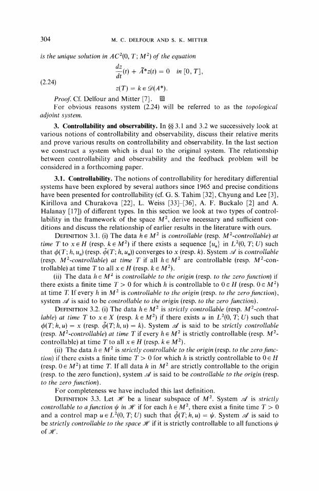
is the unique solution in AC2(0, T; M2) of the equation
(2.24)
dz--(t) + *z(t) 0 in [O, T],dt
z(T) k (A*).
Proof Cf. Delfour and Mitter [7]. k
For obvious reasons system (2.24) will be referred to as the topologicaladjoint system.
3. Controllability and observability. In 3.1 and 3.2 we successively look atvarious notions of controllability and observability, discuss their relative meritsand prove various results on controllability and observability. In the last sectionwe construct a system which is dual to the original system. The relationshipbetween controllability and observability and the feedback problem will beconsidered in a forthcoming paper.
3.1. Controllability. The notions of controllability for hereditary differentialsystems have been explored by several authors since 1965 and precise conditionshave been presented for controllability (cf. G. S. Tahim 32], Chyung and Lee 3],Kirillova and Churakova 22], L. Weiss [333-36], A. F. Buckalo [21 and A.Halanay [17]) of different types. In this section we look at two types of control-lability in the framework of the space M2, derive necessary and sufficient con-ditions and discuss the relationship of earlier results in the literature with ours.
DEFINITION 3.1. (i) The data h M2 is controllable (resp. M2-controllable) attime T to x H (resp. k M2) if there exists a sequence {u,} in L2(0, T; U) suchthat b(T; h, u,) (resp. b(T; h, u,)) converges to x (resp. k). System /is controllable(resp. MZ-controllable) at time T if all h M2 are controllable (resp. MZ-controllable) at time T to all x H (resp. k M2).
(ii) The data h M2 is controllable to the origin (resp. to the zero function) itthere exists a finite time T > 0 for which h is controllable to 0 H (resp. 0 e M2)at time T. If every h in M2 is controllable to the origin (resp. to the zero function),system ’ is said to be controllable to the origin (resp. to the zero function).
DEFINITION 3.2. (i) The data h M2 is strictly controllable (resp. MZ-controllable) at time T to x X (resp. k M2) if there exists u in La(0, T; U) such thatb(T; h, u)= x (resp. b(T; h, u)= k). System ’ is said to be strictly controllable(resp. MZ-controllable) at time T if every h m2 is strictly controllable (resp. mz-controllable) at time T to all x H (resp. k M2).
(ii) The data h m2 is strictly controllable to the origin (resp. to the zero func-tion) if there exists a finite time T > 0 for which h is strictly controllable to 0 H(resp. 0 M2) at time T. If all data h in M2 are strictly controllable to the origin(resp. to the zero function), system is said to be controllable to the origin (resp.to the zero function).
For completeness we have included this last definition.DEFINITION 3.3. Let C be a linear subspace of M2. System ’ is strictly
controllable to a function in if for each h M2, there exist a finite time T > 0and a control map u L2(0, T; U) such that (T; h, u) . System is said tobe strictly controllable to the space if it is strictly controllable to all functions Ooi’o
AFFINE HEREDITARY DIFFERENTIAL SYSTEMS 305
PROPOSITION 3.4. When H isfinite-dimensional the notion of strict controllabilityat time T (resp. strict controllability to the origin) is equivalent to the notion ofcontrollability at time T (resp. controllability to the origin).
In this paper we shall not consider the "strict" notions unless we are in thesituation of Proposition 3.4. The following results are obtained directly from thedefinitions.
PROPOSITION 3.5. (i) is never strictly MZ-controllable at time T.(ii) For all T < b, is never MZ-controllable at time T or controllable to
the zero function.(iii) The controllability of e’ at time T is a necessary condition for the mz-
controllability of at time T. kRemark. (i) When b- , ’ is never controllable to the zero function or
M2-controllable at any finite T => 0.(ii) Proposition 3.5 (i) implies that when is MZ-controllable at time T,
the initial states in m2 are only strictly controllable to points in a dense subspaceof M2 which is different from M2.
PROPOSITION 3.6. is controllable to the origin (to the zero function) if thereexists afinite time T > 0 such that ’ is controllable (MZ-controllable) at time T. k
Remark. A similar statement is true for the "strict" notions.All the above definitions were originally given in the literature for initial
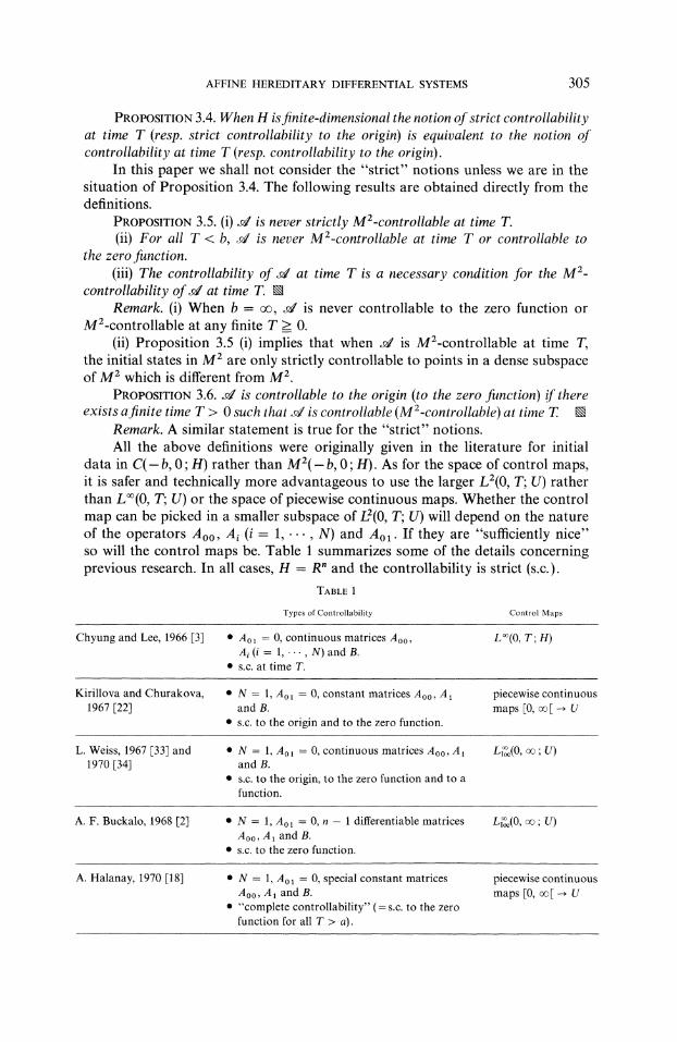
data in C(-b, 0;H) rather than m2(-b, 0;H). As for the space of control maps,it is safer and technically more advantageous to use the larger L2(0, T; U) ratherthan L(0, T; U) or the space of piecewise continuous maps. Whether the controlmap can be picked in a smaller subspace of L2(0, T; U) will depend on the natureof the operators Aoo, Ai (i 1, ..., N) and Aol. If they are "sufficiently nice"so will the control maps be. Table 1 summarizes some of the details concerningprevious research. In all cases, H R" and the controllability is strict (s.c.).
TABLE
Types of Controllability Control Maps
Chyung and Lee, 1966 [3] Aol 0, continuous matrices Aoo,Ai (i 1, ..., N) and B.s.c. at time T.
L(O, T; H)
Kirillova and Churakova,1967 [22]
N 1, Aol 0, constant matrices Aoo, Aand B.s.c. to the origin and to the zero function.
piecewise continuousmaps [0, [ U
L. Weiss, 1967 [333 and1970 [34]
N 1, A0 0, continuous matrices Aoo, Aand B.s.c. to the origin, to the zero function and to a
function.
L%(0, oe’U)
A. F. Buckalo, 1968 [21 N 1, Ao 0, n differentiable matricesAoo, A and B.s.c. to the zero function.
L(O, ’U)
A. Halanay, 1970 [18] N 1, Aol 0, special constant matricesAoo, A and B."complete controllability" (= s.c. to the zerofunction for all T > a).
piecewise continuousmaps [0, [ U
306 M.C. DELFOUR AND S. K. MITTER
Definitions 3.1 (ii), (3.2) (ii) and 3.3 are conceptually interesting but technicallydifficult to deal with since thefinal time T is not fixed. Even from the engineeringstandpoint it is desirable to have a uniform bound on T independent of the initialdata h in M2. In fact, most conditions for "controllability of Definitions 3.1 (ii),3.2 (ii) and 3.3" are only sufficient. They make use of Proposition 3.6, the converseof which is obviously not true. The notion of MZ-controllability is new in thecontext of hereditary differential systems, though the idea of density has oftenbeen used in partial differential equations where it naturally arises. It is clearthat at time > 0 the state (t; h, u) will be absolutely continuous in [-t, 0](see (2.7)). Thus it will be impossible to synthesize an MZ-map or even a continuousmap defined in I(-b, 0) which is not at least differentiable in the interval [-t, 0].For all the above reasons we shall limit the scope of our investigation to thenotions of controllability of Definitions 3.1 (i) and 3.2 (i).
THEOREM 3.7. The following statements are equivalent"(i) 1 is controllable (resp. MZ-controllable) at time T;(ii) the map u-- S(T)u (T, s)B(s)u(s)ds:L2(O, T; U)- H (resp. u
(T)u r ~ofo (T,s)B(s)u(s)ds:L2(O, T; U)-M2(-b,O;H))hasadenseimage in H (resp. M2( b, 0; H));
(iii) the map x-- S(T)*x’H L2(0, T; U) (resp. k-- VS(T)*k’mZ(-b, 0; H)L2(0, T; U)), where (S(T)*x)(t)= B(t)*(T, t)*x (resp. ((T)*k)(t)B(t)*(T, t)*k), is injective;
(iv) the symmetric operator
W(T) O(T, s)B(s)B(s)*(T, s)* ds
(resp. I(T) O(T, s)B(s)B(s)* O(T, s)* ds)is positive definite.
Proof. This is a corollary to Delfour and Mitter [11, Thm. 9 and Cor. 10].COROLLARY 3.8. Let H R". (i) The condition
(3.1) rank (W(T)) n
is necessary and sufficient for the strict controllability of1 at time T.(ii) Condition (3.1) is necessary for the MZ-controllability of t’ at time T.(iii) If there exists a time T, 0 <= T < , for which condition (3.1) holds, then
system d’ is strictly controllable to the origin. []
Remark. Part (i) of the corollary is due to Chyung and Lee [3] and part (iii)to L. Weiss [33, Lemma 1].
PROPOSITION 3.9. Assume there exists T, 0 < T < ,such that Im (D(T, 0)) H.If all initial states h M2 are controllable to the origin at time T, system 1 iscontrollable at time T.
Proof. For all h M2, x H there exists k M2 such that
(3.2) x + ,(T, 0)h ,(T, 0)k.
Since ’ is controllable to the origin at time T there exists {u,} in L2(0, T; U) suchthat
(3.3) (T, 0)k + O(T, s)B(s)u,(s) ds + ap(T, s)f(s) ds - O.
AFFINE HEREDITARY DIFFERENTIAL SYSTEMS 307
Hence sO’ is controllable at time T by combining (3.2) and (3.3). k
Remark. The condition Im ((T, 0))= H is equivalent to have the "forcefree attainable set"
{tI)(T, O)h[h M2
equal to H. When the property is true for all T > 0, then system sO’ is said to bepointwise complete. This definition is due to L. Weiss [33] who conjectured thatfor H R" all systems of the form
dx--(t) Aox(t)+ Alx(t-a) + Bu(t), >=0,dt
x(s) h(s), s e [-a, O],
are pointwise complete. This point has been investigated by V. M. Popov [29]who has shown that the conjecture is false for n > 2. Popov has further foundnecessary and sufficient conditions for the system to be pointwise complete.
Finally we restrict our attention to H R" and systems of the form
(3.4)
dx--(t) Ao(t)x(t + A(t)x(t a) + B(t)u(t) + f(t), >= O,dt
x(s) h(s), s e [-a, O],
where Ao and A are in Lc(0, o (R")), B e Lc(0, (R", R")) andfe L2(0, ;R"). Notice that
and that for T >__ a,
t(t, O) Ao(t)(t, 0),
(o, o)
e [0, a],
c(T,s) + (T,s)Ao(s)=0, s[T- a, T],s
(3.6)(T, T)= I.
This means that the force free attainable set is equal to R" in the interval [0, a] since
R" Im ((t, 0)) Im ((t, 0)) R".
Also, we have the following proposition.PROPOSITION 3.10. (i) If there exists To IT- a, T f-) [0, T] for which the
system
dx--(t) Ao(t)x(t + B(t)u(t), [To, T],dt
is strictly controllable at time T, then system xal is strictly controllable at time T.(ii) If in addition Ao and B are respectively n 2 and n 1 times continuously
differentiable in [T0, T], we can construct the controllability matrix of Silverman
308 M. C. DELFOUR AND S. K. MITTER
and Meadows [31]
where
Qc(t) [Po(t)iPa(t)i
Pk + (t) Ao(t)Pk(t) + P(t),
Po(t) B(t),
and the condition of part (i) is equivalent to the existence of some [To, T] forwhich rank Qc(t) n.
Remark. A. F. Buckalo [2] used the condition of L. Weiss and incorporatedthe ideas of Silverman and Meadows 31] to essentially obtain part (ii) of the aboveproposition. The classical rank condition is obtained when the matrices Ao andB are not time dependent.
In addition to the above results one should mention the work of Kirillovaand Churakova [22] and L. Weiss [34]. It is the first attempt to obtain directconditions on the various matrices in contrast to the above results where the(strict) controllability of a nonhereditary system serves as a sufficient conditionfor the (strict) controllability of s’.
3.2. Observability. To our knowledge the notion of observability for HDShas not been studied in the published literature. We have seen that there areseveral notions of controllability. Likewise, there are more than one way toobserve system s’ and different things to observe.
Let Y be a Hilbert space which might be thought of as the observation space.We can observe the map qS(. h, u) with an observer Z L(O, T; ’(H, Y));the observation at time is defined by
(3.7) z(t; h, u) Z(t)dp(t; h, u).
We can also observe the map (. ;h,u) with an M2-observer eL(O, T;5(M2, Y)); the M2-observation at time is defined by
(3.8) Y,(t; h, u) (t))(t; h, u).
Since M2(-b,O;H) is isomorphic to H x L2(-b,O;H), there exist ,(t)2,(’(H, Y) and ,a(t) 5(L2( b, 0; H), Y) such that
(3.9) (t)(t-a(h, 0)) (t)hand
(3.10) (t)(t-a(0, ha))
Notice that our observer satisfies hypothesis (ii) in Definition 12 (cf. Delfour andMitter [11]). Now starting from either of the above two types of observations, wecan either determine the state h M2(-b, 0; H) or simply h H.
DEFINITION 3.11. (i) System 1 is observable in [0, T] if for all h M2(- b, 0; H)and u L2(0, T; U) the point h H can be uniquely determined from a knowledgeof u, h and the observation map z(. ;h, u), where x(h)= (h, h a) and x is theisometric isomorphism between MZ( b, 0;H) and H LZ(-b, 0;H).

AFFINE HEREDITARY DIFFERENTIAL SYSTEMS 309
(ii) System ’ is strongly observable in [0, T] if for all h M2( b, 0;H) andu L2(0, T; U), the state h can be uniquely determined from a knowledge of uand the observation map z( h, u).
(iii) System ’ is MZ-observable in 0, T] if for all h MZ(-b, 0; H) andu L2(0, T; U) the state h can be uniquely determined from u and the observationmap (. h, u).
PROPOSITION 3.12. Let 2(t) Z(t).(i) strongly observable ’ M2-observable and observable.
(ii) For all T < b, ’ is not strongly observable in [0, T].Proof. The proof follows from the definitions.Remarks. (i) When b , system is never strongly observable in [0,
for all finite T.(ii) When ,a(t) 0, strong observability and M-observability are equivalent.PROPOSITION 3.13. The following statements are equivalent:(i) ’ is observable in [0,(ii) the map F :U L2(0, T; Y), where ((F)h)(t) Z(t)@(t, O)h, is in-
jective(iii) the map y- (F)*y (t, O)*Z(t)*y(t) dt "L2(0, T; Y) H has a dense
image in H;(iv) the symmetric operator
(3.11) W(T) (t, O)*Z(t)*Z(t)O(t, O) dt
is positive definite.Proof. The proof is similar to the proof of Theorem 3.7.COROLLARY 3.14. Let H R". (i) The condition
(3.12) rank (W(T)) n
is necessary and sufficient for the observability of in [0, T].(ii) Condition (3.12) is necessary for strong observability of systemProof. The proof is similar to the proof of Corollary 3.8.COROLLARY 3.15. Consider the system of equations (3.4) with observer
Z L(O, T; (R", Y)).(i) If there exists T [0, T] CI [0, a] for which the system
dxd--[(t) + Ao(t)*x(t + Z(t)*y(t) 0 in [0, Tf],
x(rf) h
is controllable at time 0, then system s is observable in [0, T].(ii) If in addition Ao and Z are respectively n 2 and n 1 times continuously
differentiable in [0, Ty], we can construct the observability matrix ofSilverman and Meadows [31],
(3.13) Qo(t) [So(t)iS(t)!. !S,_ (t)],
where
Sk+ x(t) Ao(t)*S(t + (t), So(t)- Z(t)*,(3.14)
310 M. C. DELFOUR AND S. K. MITTER
and the condition ofpart (i) is equivalent to the existence of some [0, Tj.]for which rank (Qo(t)) n. k
Remark. The classical rank condition is obtained when the matrices Ao andZ are not time dependent.
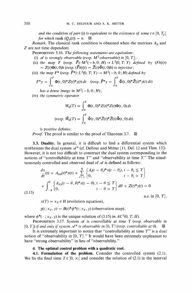
PROPOSITION 3.16. The following statements are equivalent"(i) ’ is strongly observable (resp. MZ-observable) in [0, T];
(ii) the map F (resp. )’mz(-b,O;H) L2(0, T; Y) defined by (Fh)(t)Z(t)(t, O)h (resp. (h)(t) 2(t)4)(t, O)h) is injective;
(iii) the map F* (resp. lff*)’L2(0, T; Y) -- m2( b, 0;H) defined by
F*y (I)(t, O)*Z(t)*y(t)dt (resp. l*y (t, O)*(t)*y(t)at)
has dense image in M( b, O;H);(iv) the symmetric operator
Wo(T) (t, O)*Z(t)*Z(t)(t, O)dt
(resp. lo(T) (t, 0)*2(t)*2(t)(t, 0)
is positive definite.Proof. The proof is similar to the proof of Theorem 3.7.
3.3. Duality. In general, it is difficult to find a differential system whichsynthesizes the dual system ’* (cf. Delfour and Mitter [11, Def. 12 and Thm. 13]).However, it is not too difficult to construct the dual system corresponding to thenotions of "controllability at time T" and "observability at time T." The simul-taneously controlled and observed dual of ’ is defined as follows:
dXd__{(t + Aoo(t),x(t)+ N Ai(t Oi),x(t Oi),t Oi <= TT}(o, o >i=
ff {Aol(t-O O)*x(t-O),t-O<-T}do+Z(t),y(t)= 0O, t-O> T
x(T) xT H (evolution equation),
X(t xT, Y) B(t)*ck*(t xr, y) (observation map),
where b*(. ;XT, Y) is the unique solution of (3.15) in AC2(0, T; H).
a.e. in [0, T],
PROPOSITION 3.17. System s’ is controllable at time T (resp. observable in[0, T]) if and only if system s/* is observable in [0, T] (resp. controllable at 0). k
It is extremely important to notice that "controllability at time T" is a dualnotion of "observability in [0, T]." It would have been extremely unpleasant tohave "strong observability" in lieu of "observability."
4. The optimal control problem with a quadratic cost.4.1. Formulation of the problem. Consider the controlled system (2.1).
We fix the final time T ]0, [ and consider the solution of (2.1) in the interval
AFFINE HEREDITARY DIFFERENTIAL SYSTEMS 311
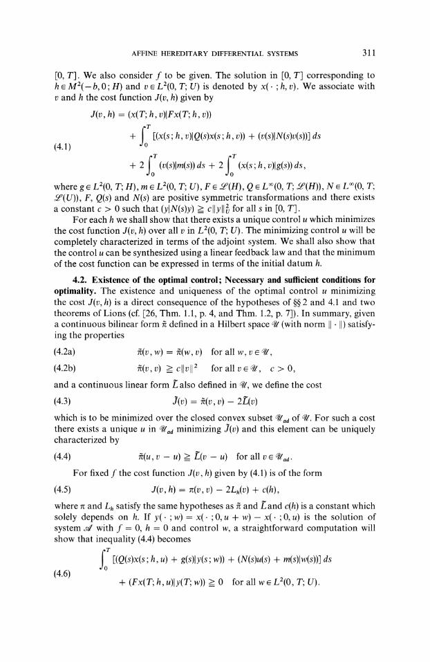
[0, T]. We also consider f to be given. The solution in [0, T] corresponding toh M2( b, 0; H) and v L2(0, T; U) is denoted by x(. h, v). We associate withv and h the cost function J(v, h) given by
J(v, h) (x(T; h, v)lFx(T; h, v))
+ [(x(s; h, v)lQ(s)x(s;h, v)) + (v(s)lg(s)v(s))] ds
+ 2 (v(s)lm(s)) ds + 2 (x(s; h, v)lg(s)) ds,
where g L2(0, T; H), m L2(0, T; U), F q(H), Q L(0, T; 5(H)), N L(0, T;2’(U)), F, Q(s) and N(s) are positive symmetric transformations and there existsa constant c > 0 such that (ylN(s)y) > c y for all s in [0, T].
For each h we shall show that there exists a unique control u which minimizesthe cost function J(v, h) over all v in L2(0, T; O). The minimizing control u will becompletely characterized in terms of the adjoint system. We shall also show thatthe control u can be synthesized using a linear feedback law and that the minimumof the cost function can be expressed in terms of the initial datum h.
4.2. Existence of the optimal control; Necessary and sufficient conditions foroptimality. The existence and uniqueness of the optimal control u minimizingthe cost J(v, h) is a direct consequence of the hypotheses of 2 and 4.1 and twotheorems of Lions (cf. [26, Thm. 1.1, p. 4, and Thm. 1.2, p. 7]). In summary, givena continuous bilinear form defined in a Hilbert space ’ (with norm I]" I]) satisfy-ing the properties
(4.2a) (v, w) (w, v) for all w, v ’,
(4.2b) (v,/)) C V 2 for all v e , c > 0,
and a continuous linear form also defined in , we define the cost
(4.3) ,7(v) :(v, v)- 2(v)which is to be minimized over the closed convex subset ’ad of ’. For such a costthere exists a unique u in ’ad minimizing J(v) and this element can be uniquelycharacterized by
(4.4) (u,v-u)=>(v-u) for allvd.For fixed f the cost function J(v, h) given by (4.1) is of the form
(4.5) J(v, h)= re(v, v)- 2Lh(v) + c(h),
where rc and Lh satisfy the same hypotheses as and and c(h) is a constant whichsolely depends on h. If y(.; w)= x(.;0, u + w)- x(.;0, u) is the solution ofsystem s’ with f 0, h 0 and control w, a straightforward computation willshow that inequality (4.4) becomes
o[(Q(s)x(s; h, u) + g(s)ly(s;w)) + (N(s)u(s) + m(s)lw(s))-] ds
(4.6)+ (Fx(T; h, u)ly(T; w)) >= 0 for all w e L2(0, T; U).
312 M. C. DELFOUR AND S. K. MITTER
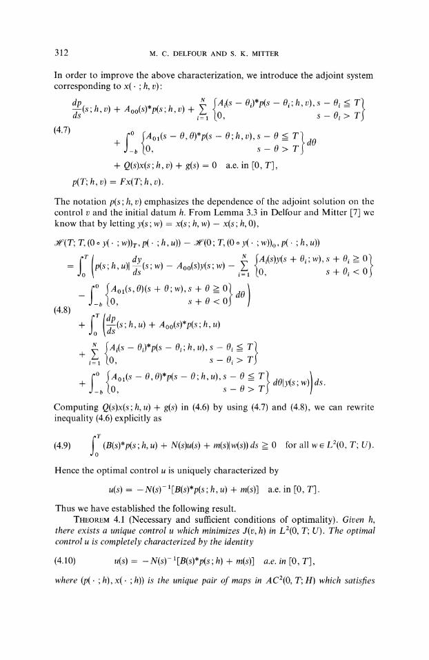
In order to improve the above characterization, we introduce the adjoint systemcorresponding to x(. ;h, v):
s; h, v) + Aoo(S)*p(s; h, v) +i= 0, s Oi >
(4.7)
f {Aoa(s-O O)*p(s-O’h v) s-O<T}d0-b O, s-O> T
+ Q(s)x(s;h, v) + g(s) 0 a.e. in [0, T],
p(T; h, v) Fx(T; h, v).
The notation p(s;h, v) emphasizes the dependence of the adjoint solution on thecontrol v and the initial datum h. From Lemma 3.3 in Delfour and Mitter [7] weknow that by letting y(s; w) x(s; h, w) x(s; h, 0),
(T; T, (0 y(. w))r, p(" ;h, u)) vf(0; T, (0 y(. W))o, p(. ;h, u))
p(s;h u)l (s; w) Aoo(S)y(s;w)= (0, s+O<_
(0, s + 0 <(4.8)
+ s; h, u) + oo(S)*p(s; h, u)
+ i:{O,n Ai(s_Oi),P(s_Oi h, u),S-s_Oi>+ dOly(s; w ds._
O, s-O>
Computing Q(s)x(s;h, u) + g(s) in (4.6) by using (4.7) and (4.8), we can rewriteinequality (4.6) explicitly as
(4.9) (B(s)*p(s; h, u) + N(s)u(s) + m(s)lw(s)) ds >= 00
for all w L2(0, T; U).
Hence the optimal control u is uniquely characterized by
u(s) N(s)- a[B(s)*p(s h, u) + m(s)] a.e. in [0, T].
Thus we have established the following result.THEOREM 4.1 (Necessary and sufficient conditions of optimality). Given h,
there exists a unique control u which minimizes J(v, h) in L2(0, T; U). The optimalcontrol u is completely characterized by the identity
(4.10) u(s) N(s)- l[B(s)*p(s h) + m(s)] a.e. in [0, T],
where (p(. ;h), x(. ;h)) is the unique pair of maps in AC2(0, T; H) which satisfies
AFFINE HEREDITARY DIFFERENTIAL SYSTEMS 313
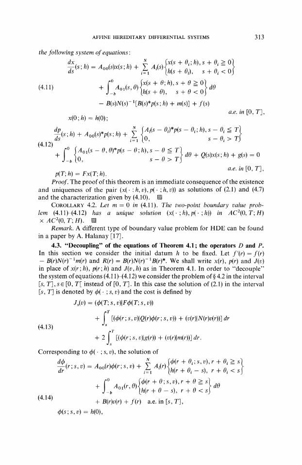
the following system of equations:
2N x(s nt- Oi; h)’s -k- Oi >=d--X(s; A(s)x(s’h)’ +i=1 .h(s + Oi) s + 0 <
(4.11) dO+ o(S, O)h(s + 0), s + 0 <
B(s)N(s)-[B(s)*p(s;h) + m(s)] + f(s)
x(0; h) h(0);a.e. in [0, T],
(4.12)
dp N fAi(S Oi),p(S Oi h), s Oi =< T(s h) + Aoo(S)*p(s h) +ds = (0, s Oi >
+ dO + Q(s)x(s;h) + g(s) 0-b O, s--O>
a.e. in [0, T],p(r; h) Fx( r; h)
Proof. The proof of this theorem is an immediate consequence of the existenceand uniqueness of the pair (x(. :h, v), p(. ;h, v)) as solutions of (2.1) and (4.7)and the characterization given by (4.10).
COROLLARY 4.2. Let m 0 in (4.11). The two-point boundary value prob-lem (4.11)-(4.12) has a unique solution (x(. ;h),p(. ;h)) in AC2(0, T;H)
AC2(0, T; H).Remark. A different type of boundary value problem for HDE can be found
in a paper by A. Halanay [17].4.3. "Decoupling" of the equations of Theorem 4.1; the operators D and P.
In this section we consider the initial datum h to be fixed. Let f’(r)= f(r)B(r)N(r)-1re(r) and R(r)= B(r)N(r)-1B(r)*. We shall write x(r), p(r) and J(v)
in place of x(r;h), p(r; h) and J(v, h) as in Theorem 4.1. In order to "decouple"the system ofequations (4.11)-(4.12) we consider the problem of{} 4.2 in the intervalIs, T], s e [0, T[ instead of [0, T]. In this case the solution of (2.1) in the intervalIs, T] is denoted by qS(. ;s, v) and the cost is defined by
Js(v) ((T; s, v)lFdp(T; s, v))
(4.13)
T
+ E(4(r ;s, v)lQ(r)dp(r ;s, v)) + (v(r)lX(r)v(r))] dr
+ 2 [(4(r; s, v)lg(r)) + (v(r)lm(r))] dr.
Corresponding to b(. ;s, v), the solution ofN d(r + O,; s, v), r + O, >= ;}dC/)dr (r s v)= Aoo(r)c/)(r s v) +
i=
Ai(r).h(r + Oi s), r + Oi <
+ Ao(r O)4)(r + O;s,v),r + 0 >
dOh(r+O-s), r+ O<
(4.14) + B(r)v(r) + f(r) a.e. in Es, T],
(s; s, v) h(O),
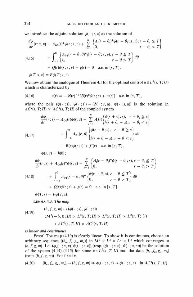
314 M. C. DELFOUR AND S. K. MITTER
we introduce the adjoint solution (. ;s, v) as the solution ofN Ai(r_Oi).(r_Oi;s,v),r_Oi<= TT}dOdr (r s v) + Aoo(r)*O(r s v) +
i= (0, r 0 >
; {Ao(r-O O)*(r-O’s v) r-O<TT}(4.5) + dOO, r-O>
+ Q(r)ck(r;s, v) + g(r) 0 a.e. in Is, T],
k(T; s, v) Fdp(T; s, v).
We now obtain the analogue of Theorem 4.1 for the optimal control u L2(s, T; U)which is characterized by
(4.16) u(r) N(r)- ’[B(r)*O(r s) + m(r)] a.e. in [s, T],
where the pair (qS(. ;s), (. ;s)) (qS(. ;s,u), (. ;s,u)) is the solution inACZ(s, T; H) x ACe(s, T; H) of the coupled system
ddP (r.s)= Aoo(r)(r.s) + Ai(r)c(r + Oi,s), r + Oi>_
dr (h(r + Oi- s) r + Oi<
fo Ic/)(r + O;s), r + O >__ s}(4.17) + Ao (r, O) dO-b [,h(r + O- s),r + O < s
R(r)O(r;s) + f’(r) a.e. in Is, T],
b(s, s) h(O);
(r;s) + Aoo(r)*O(r;s +i= (0, r Oi > T
fo O(r O s, r--O< TT} dO(4.18) + -bAl(r-- 0,0)*(0, r-- 0 >
+ Q(r)dp(r;s) + g(r) 0 a.e. in Is, T],
O(T; s) VqS(T; s).
LEMMA 4.3. The map
(h, f, g, m) (b(. ;s), 0(" ;s))(4.19)
:mz(-b, O;H) x L2(s, T;H) x L2(s, T;H) x LZ(s, T; U)- AC2(s T; H) x AC2(s T; H)
is linear and continuous.
Proof. The map (4.19) is clearly linear. To show it is continuous, choose anarbitrary sequence {(h,,f,, g,,m,)} in M2 L2 L2 L2 which converges to(h, f, g, m). Let (4,( s, v), .(. s, v)) (resp. (4)(" s, v), (. s, v))) be the solutionof the system (4.14)-(4.15) for some v e L2(s, T; U) and the data (h,,f,, g,, m,)(resp. (h, f, g, m)). For fixed v,
(4.20) (h,, L, g,, m,) --, (h, j; g, m) b,(. s, v) -+ 05(. s, v) in ACe(s, T; H)
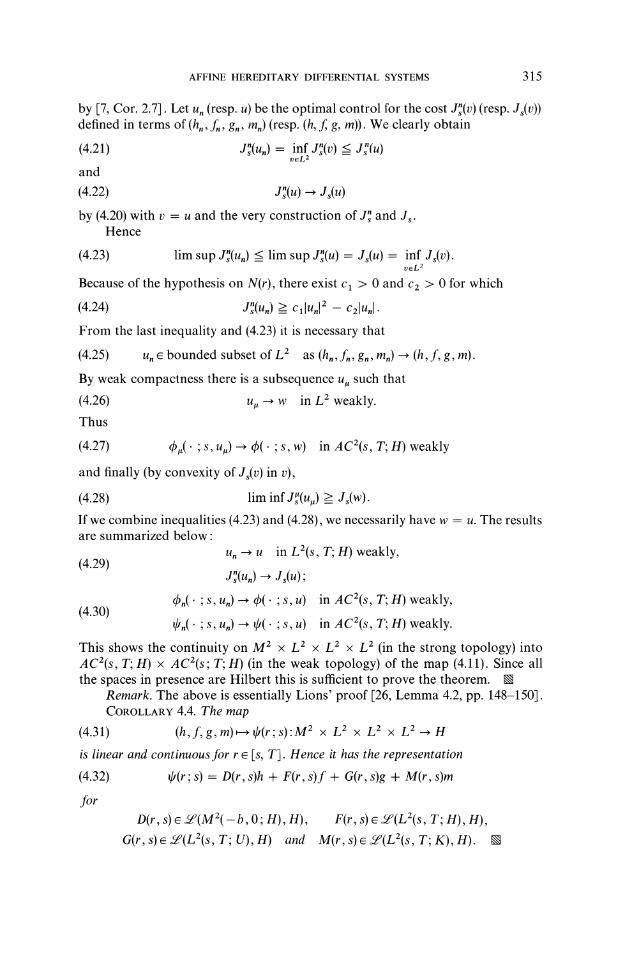
AFFINE HEREDITARY DIFFERENTIAL SYSTEMS 315
by [7, Cor. 2.7]. Let u, (resp. u) be the optimal control for the cost J"(v) (resp. Js(v))defined in terms of (h,, f,, g,, m,) (resp. (h, f, g, m)). We clearly obtain
(4.21) J’(u,) inf J’(v) < J"(u)vL
and
(4.22) J(u)--, Js(u)
by (4.20) with v u and the very construction of J" and J.Hence
(4.23) lim sup J(u,) <= lim sup J(u) J(u) inf J(v).vL
Because of the hypothesis on N(r), there exist c > 0 and c2 > 0 for which
(4.24) d’(u,) > clu,l 2 c21u,l.
From the last inequality and (4.23) it is necessary that
(4.25) u, bounded subset of n2 as (hn, fn, gn, ran) -- (h, j g, m).
By weak compactness there is a subsequence u, such that
(4.26) uu --, w in L2 weakly.
Thus
(4.27) dpu s, uu) -, q5( s, w) in AC2(s, T; H) weakly
and finally (by convexity of J(v) in v),
(4.28) lim inf d(uu) >= ds(w).
If we combine inequalities (4.23) and (4.28), we necessarily have w u. The resultsare summarized below:
(4.29)u, --, u in L2(s, T; H) weakly,
Jn(U,) J(u);
b,(. ;s, u,) --* q)(" ;s, u) in AC2(s, T; H) weakly,(4.30)
,(. ;s, u,) - p(. ;s, u) in AC2(s, T; H) weakly.
This shows the continuity on M2 L2 L2 L2 (in the strong topology) intoAC2(s, T; H) AC2(s; T; H) (in the weak topology) of the map (4.11). Since allthe spaces in presence are Hilbert this is sufficient to prove the theorem, k
Remark. The above is essentially Lions’ proof [26, Lemma 4.2, pp. 148-150].COROLLARY 4.4. The map
(4.31) (h,f,g,m)---d/(r;s):M2 L2 L2 x L2--* H
is linear and continuous jbr r [s, T]. Hence it has the representation
(4.32) 6(r; s)= D(r, s)h + F(r, s)f + G(r, s)g + M(r, s)m
foD(r, s) e (M2(- b, 0; H), H), F(r, s) e .q(L2(s, T; H), H),
G(r, s) (L2(s, T; U), H) and M(r, s) (L2(s, T; K), U). k
316 M. C. DELFOUR AND S. K. MITTER
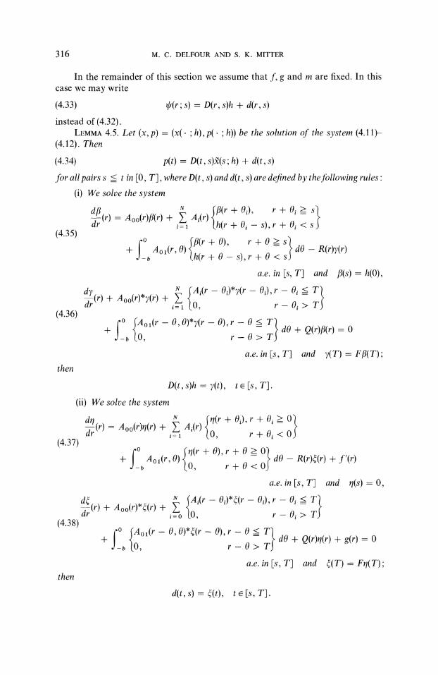
In the remainder of this section we assume that f, g and m are fixed. In thiscase we may write
(4.33) O(r; s) D(r, s)h + d(r, s)
instead of (4.32).LEMMA 4.5. Let (x, p) (x(. ;h), p(. ;h)) be the solution of the system (4.11)-
(4.12). Then
(4.34) p(t) D(t, s)2(s h) + d(t, s)
for all pairs s <= in [0, T], where D(t, s) and d(t, s) are defined by thefollowing rules"
(i) We solve the system
(r) Aoo(r)fl(r) + Ai(ri= (h(r + Oi- s),r + Oi < s
(4.35)
fo ffi(r + o), r + O >_ s}+ Aol(r, O) dO R(r)y(r-b (h(r + O- s),r + O < s
a.e. in Is, T] and fl(s) h(O),
dTdr (r)+ Aoo(r)*7(r) + _,N Ai(r_Oi),7(r_Oi),r_Oi<= ;}1 (0, r 0 >
(4.36) ;o {Aol(r O,O),7(r O) r O < ;}+ o + 2(r)/(O 0-b O, r--O>
a.e. in [s, r] and ?( T) F(T)then
D(t, s)h ?(t),
(ii) We solve the system
(4.37)
(4.38)
then
te[s, T].
(r) Aoo(r)rl(r) + Ai(r(0, r+Oi>=2}r+Oi<
q-- Aol(r, O) dO R(r)(r) + f’(r)-b 0, r + 0 <
a.e. in Is, T] and r/(s) O,
+ Aoo(r)*(r) +o o, r 0 >
;: o 0, 0+ dO + Q(r)(r)+ g(r)= 0
0, r-0>
a.e. in [s, r and (T) F(T)
d(t,s) (t), e Is, T].

AFFINE HEREDITARY DIFFERENTIAL SYSTEMS 317
Proof. D(t, s) and d(t, s) are clearly obtained from the rules (i) and (ii) of thelemma" it suffices to decompose the map h O(r) into its linear part and its con-stant part. We only need to establish identity (4.34). Consider the system (4.14)-(4.15) with initial datum 2(s; h) (see Definition 2.1) at time s, where x is the solutionof the system (4.11)-(4.12) with initial datum h. The solution is denoted by (4, ).
We also define
q5 (resp. ) restriction of x (resp. p) to Is, T],
where b and are the solutions of the system (4.14)-(4.15) with initial datum2(s h). By uniqueness, (4), 0) (b, 0) and p(t) O(t) D(t, s)2(s h) + d(t, s).This proves the lemma. KN
Remark. The above is essentially Lions’ original proof (cf. J. L. Lions [26,Lemma 4.3]).
COROLLARY 4.6. Given s [0, T[ and h M2(-b, 0;H), the maps D(t, s)hand d(t, s) are in AC2(s, T; H). kN
DEFINITION 4.7. For all s [0, T[ and r/ I(-b, 0), s r/=< T, let
(D(s rl, s), rl Is T, 0] f"l I(-b, 0),(4.39) P(s, r/) ’((0, otherwise.
This defines the operator P(s)e (M(-b, 0; H)) in the natural way (P(s)h)(rl)P(s, rl)h. Similarly, let
d(s q, s), e [s r, o] ["lI(-b,0),(4.40) r(s,r/)
0, otherwise;
and this defines r(s) e M2(- b, 0; H), where (r(s))(r/) r(s, rl).Remark. The conclusions of Lemma 4.5 can also be written in state form.
Let 2,/, p and denote the state variables associated with the variables x, p, 7and , respectively. We can write/(s) P(s)2(s) + r(s), where P(s)h p(s) andr(s) (s). Here P(s) and r(s) are defined directly.
4.4. The operator H(s) and the optimal cost; relations between H and P.In this section we introduce the operator H(s) which characterizes the optimal cost.It is constructed from D(s rl, s), rl e I(-b, 0), s rl <= T, or simply from P(s, r/)(Definition 4.5). Since there is an isometric isomorphism between M2(-b, 0;H)and H x L2(-b, 0;H) the operator P(s, rl) can be decomposed in the followingway"
(4.41) P(s, rl)h P(s, rl)h + PX(s, rl)h a,where h M2(-b, 0; H), to(h)= (h,h) (see [6, Prop. 2.1]), P(s, rl)e 2’(H) andP(s, ) e (CZ(- b, 0; H), H).
PROPOSITION 4.8. Let f g 0 and m 0 in system (4.17)-(4.18). We denoteby (b(. ;s), (. s))(resp. ((. ;s), (. ;s))) its solutionfor the initial datum h (resp. ).Then
W(s; r,h,D(.,s)h) (c(r;s)lVp(r;s)) + [((r;s)lR(r)O(r;s))(4.42)
+ (Q(r)c/)(r;s)[c/)(r;s))] dr.
318 M. C. DELFOUR AND S. K. MITTER
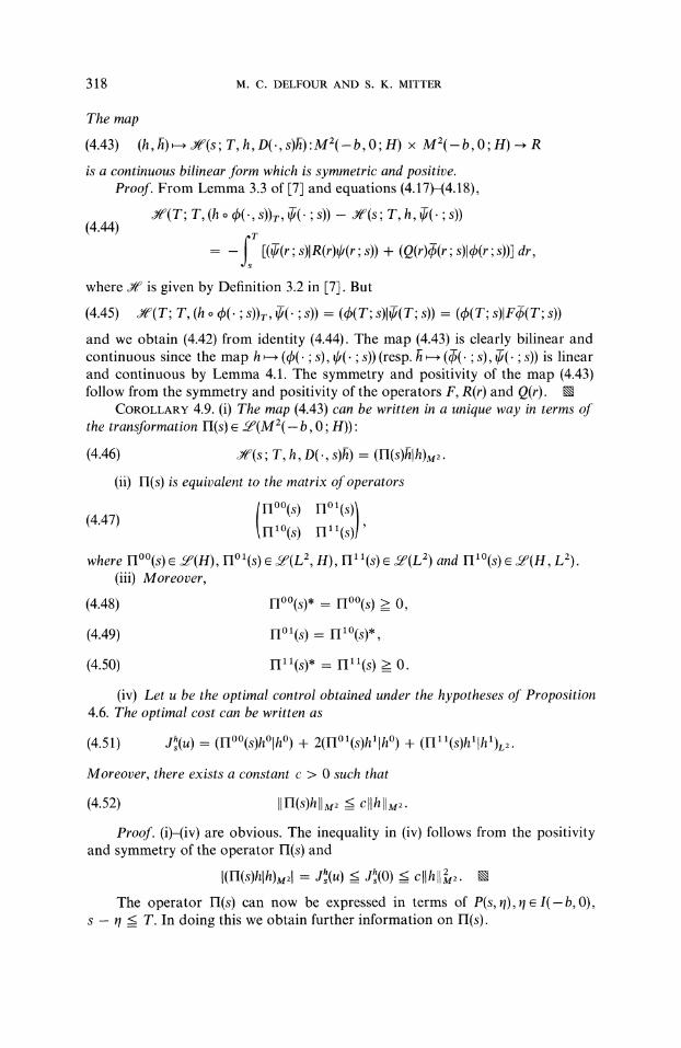
The map
(4.43) (h, )- Vf(s; T, h, D(., s))’M2(- b, 0; H) x M2(- b, 0; H) R
is a continuous bilinear form which is symmetric and positive.Proof. From Lemma 3.3 of [7] and equations (4.17)-(4.18),
’(T; T, (h qb(., s))r, O(" s)) d4’(s T, h, O(" s))(4.44)
[(O(r; s)lR(r)O(r; s)) + (Q(r)(r s)l(r;s)) dr,
where is given by Definition 3.2 in [7. But
(4.45) (T; r, (h 4(. s)), O( ;s)) ((r; s)lO(r; s)) (4(r; s)lF4(r; s))
and we obtain (4.42) from identity (4.44). The map (4.43) is clearly bilinear andcontinuous since the map h ((. s), O(" s)) (resp. h ((. s), O(" s)) is linearand continuous by Lemma 4.1. The symmetry and positivity of the map (4.43)follow from the symmetry and positivity of the operators F, R(r) and Q(r). N
COROLLARY 4.9. (i) The map (4.43) can be written in a unique way in terms ofthe transformation H(s) e (M2(- b, 0; H))"
(4.46) (s; T, h, D(., s)) (n(s)h).
(ii) (s) is equivalent to the matrix of operators
nOO(s) nol(s)(4.47) n(s) n(s)l’where (s) e (H), H(s) e (L2, H), (s) e (L2) and H(s) e (H, L2).
(iii) Moreover,
(4.48) n(s)* H(s) 0,
(4.49) n (s) n (s)*,
(4.50) n(s)* n(s) 0.
(iv) Let u be the optimal control obtained under the hypotheses of Proposition4.6. The optimal cost can be written as
(4.51) J(u) (n(s)hh) + 2(n(s)hlh) + (n(s)hllh).
Moreover, there exists a constant c > 0 such that
(4.52) IIn(s)hllM cllhl M.
Proof. (i)-(iv) are obvious. The inequality in (iv) follows from the positivityand symmetry of the operator 1-I(s) and
[(II(s)h[h)M2[ dhs(u <_ das(O) <__ c[[h t2. k
The operator FI(s) can now be expressed in terms of P(s, rl), rl e I(-b, 0),s r/=< T. In doing this we obtain further information on Fl(s).
AFFINE HEREDITARY DIFFERENTIAL SYSTEMS 319
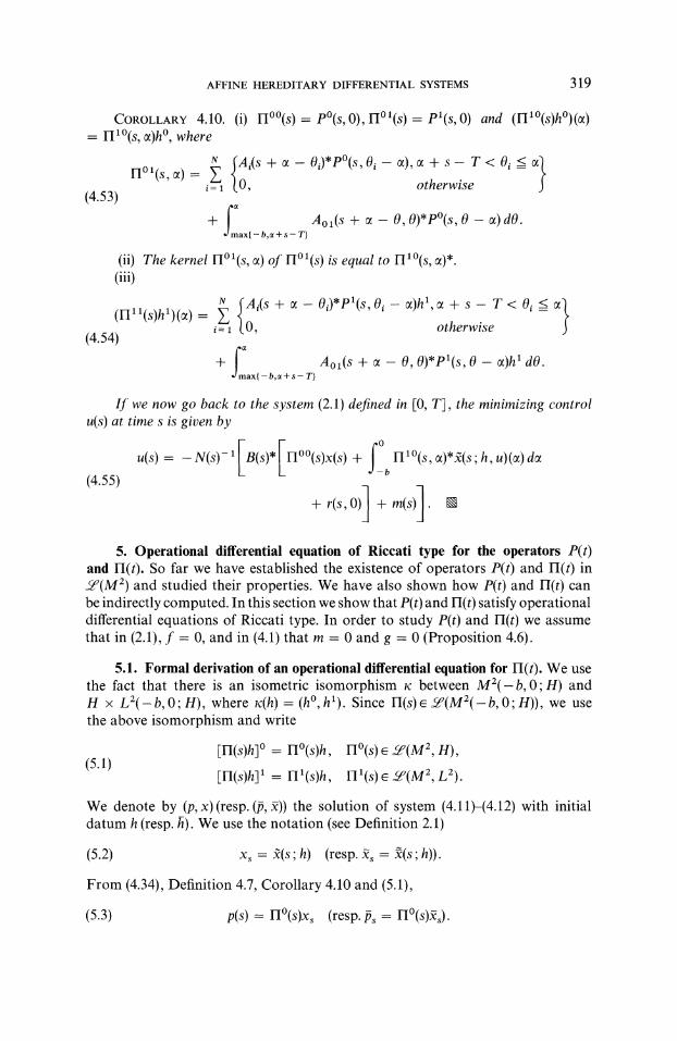
COROLLARY 4.10. (i) Fl(s) P(s, 0), I-ll(s) P(s, O) and (II(s)h)(a)II (s, a)h, where
N Ai(s + z Oi)*P(s, Oi- z), + s- r < Oi <rl (s, ) Y.
i- I.O, otherwise(4.53)
Ym+ Ao (s + O, O)*P(s, 0 cz) dO.ax{ b, + T}
(ii) The kernel gIl(s, cz) of 1-I l(s) is equal to FI (s, )*.(iii)
{ A’(s + O’)*P’(s’O’ z)hl z + s T < O’ <(1-Il(s)h)(z)i- 0, otherwise
(4.54)
f2+ Ao(S + o O, O)*P(s, 0 oOh dO.ax{ b,o + T}
If we now go back to the system (2.1) defined in [0, T], the minimizing controlu(s) at time s is given by
(4.55)u(s)=-N(s)-I,(s)*[rI(s)x(s)+ f] I-IX (s, e)*2(s h, u)(e) de
+r(s,0)] + m(s)].5. Operational differential equation of Riccati type for the operators P(t)
and 1-I(t). So far we have established the existence of operators P(t) and FI(t) in(Me) and studied their properties. We have also shown how P(t) and FifO canbe indirectly computed. In this section we show that P(t) and FI(t) satisfy operationaldifferential equations of Riccati type. In order to study P(t) and FI(t) we assumethat in (2.1), f 0, and in (4.1) that m 0 and g 0 (Proposition 4.6).
5.1. Formal derivation of an operational differential equation for II(t). We usethe fact that there is an isometric isomorphism x between Me(-b, 0; H) andH x Le(-b, 0; H), where x(h) (h,h). Since II(s)e 2’(Me(-b, 0; H)), we usethe above isomorphism and write
[n(s)h] 1-I(s)h,
[n(s)h3 Hl(s)h,
Fl(s) e &(M2, H),
I-I l(s) &a(M2, L2).
We denote by (p, x) (resp. (,2)) the solution of system (4.11)-(4.12) with initialdatum h (resp. h). We use the notation (see Definition 2.1)
(5.2) Xs 2(s;h) (resp. ffs (s;h)).
From (4.34), Definition 4.7, Corollary 4.10 and (5.1),
p(s) 1-I(S)Xs (resp./s lq(s)ffs)

320 M. C. DELFOUR AND S. K. MITTER
Define operators/(t), O(t) and/ in (M2) as
R(t)h(O),(5.4) [/(t)h](z)(0,
Q(t)h(O),(5.5) [O(t)h]()(0,
Fh(O),(5.6) [h](a)(0,
It is easy to verify the following:
(5.7)
and
(5.8)
(5.9)
(5.0)
Then from (2.16) in Theorem 2.3, (4.34) and (5.4),
dxt= (t)xt- (t)H(t)x,dt
(5.11)Xo h.
a--0,
otherwise;
otherwise;
5 O,otherwise.
[-(t)H(t)xt](O R(t)H(t)xt R(t)p(t),
(p(t)lR(t)(t))H (H(t)x,IR(t)H(t)t),
(x(T)IF(T))n (XTIT)M,
(x(t)lQ(t)(t))n (XtlO(t)t)M"
[0, T],
Formal differentiation of both sides of (5.12) and use of (5.11) yields
([l(s) + r(s)(s) + (s)*n(s) n(s)(s)n(s) + O.(s)]xl) o.Since this has to be true for all x and , we get
1() + n()() + ()*n()- n(s)()rI() + 0()= 0,(.)
H(T) ,where (s)* is the M2-adjoint of (s).
5.2. Interpretation of equation (5.14). The first question is to determine inwhat sense equation (5.14) has a solution. There are two ways to proceed" either tostudy (5.14) directly or to study an equivalent integral equation. In the first situa-tion we can apply certain results of Da Prato 4], but we need further assumptions.
(XTIrI(T)gT) (XTIFgT).
and
Equations (5.4) through (5.11) can also be written with h and in place of h and x.From (4.42), (4.46) and (5.8),
(5.12) (x,lrI(s)xs) (XTIT) + [(X10(r)) + (H(r)x,l(r)H(r))] dr
AFFINE HEREDITARY DIFFERENTIAL SYSTEMS 321
In the second situation we study an equivalent integral equation rather than thedifferential equation directly.
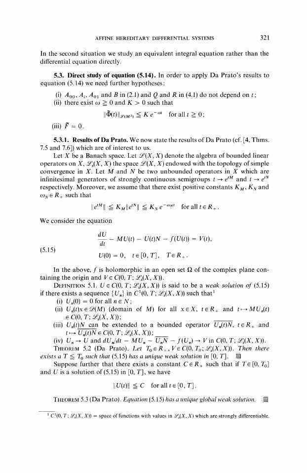
5.3. Direct study of equation (5.14). In order to apply Da Prato’s results toequation (5.14) we need further hypotheses"
(i) Aoo, Ai, Aol and B in (2.1) and Q and R in (4.1) do not depend on t;(ii) there exist co => 0 and K > 0 such that
O(t) (M2)_--<Ke ,t for allt>O;
(iii) F 0.
5.3.1. Results of Da Prato. We now state the results of Da Prato (cf. [4, Thms.7.5 and 7.6]) which are of interest to us.
Let X be a Banach space. Let (X, X) denote the algebra of bounded linearoperators on X, 2s(X, X) the space (X, X) endowed with the topology of simpleconvergence in X. Let M and N be two unbounded operators in X which areinfinitesimal generators of strongly continuous semigroups - eTM and --, etN
respectively. Moreover, we assume that there exist positive constants KM, Ku andcou R+ such that
e*Mll KMIIe K e-’"’ for all tR+.
We consider the equation
dUdt
MU(t)- U(t)N- f(U(t))= V(t),
U(O) =0, te[O,T], TeR+.
In the above, f is holomorphic in an open set f of the complex plane con-taining the origin and V C(O, T; s(X, X)).
DEFINITION 5.1. U C(O, T; s(X, X)) is said to be a weak solution of (5.15)if there exists a sequence U,} in C1(0, T; LZs(X, X)) such that
(i) U,(0) 0 for all n e N;(ii) U,(t)x (M) (domain of M) for all x X, R+ and t-- MU,(t)
e C(0, T; s(X, X));(iii) U,(t)N can be extended to a bounded operator U,(t)N, teR+ and
t- U.(t)N e C(O, T; c.qs(X, X));(iv) U, - U and du./dt MU. U.N f(U.) v in c(o, T; 5s(X, X)).THEOREM 5.2 (Da Prato). Let TO e R +, Ve C(0, To; 5Ps(X, X)). Then there
exists a T <= To such that (5.15) has a unique weak solution in [0, T]. KNSuppose further that there exists a constant C e R+ such that if T e [0, To]
and U is a solution of (5.15) in [0, T], we have
u(t)ll <-_ C for allte[O,T].
THEOREM 5.3 (Da Prato). Equation (5.15) has a unique global weak solution.
C1(0, T" Ls(X, X)) space of functions with values in 5s(X, X) which are strongly differentiable.
322 M.C. DELFOUR AND S. K. MITTER
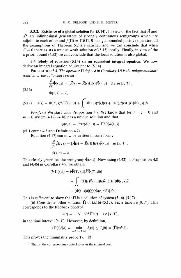
5.3.2. Existence of a global solution for (5.14). In view of the fact that A andA* are infinitesimal generators of strongly continuous semigroups which areadjoint to each other and f(I-l) I-I/l-l,/ being a bounded positive operator, allthe assumptions of Theorem 5.2 are satisfied and we can conclude that whenF 0 there exists a unique weak solution of (5.15) locally. Finally, in view of thea priori bound (4.52) we can conclude that the local solution is also global.
5.4. Study of equation (5.14) via an equivalent integral equation. We nowderive an integral equation equivalent to (5.14).
PROPOSITION 5.4. The operator I-I defined in Corollary 4.9 is the unique minimale
solution of the following system"
r(r, s) IA"(r) (r)H(r)](r, s) a.e. in Is, T],
(5.16)(s, s) I,
T
(5.17) 1-I(s) (T, s)*(T, s) + (r, s)*[0(r) + lq(r)(r)I-I(r)](r, s) dr.
Proof. (i) We start with Proposition 4.8. We know that for f g 0 andm 0 system (4.17)-(4.18) has a unique solution and that
if(r, s) P(r)@r, s) II(r)@r, s)
(cf. Lemma 4.5 and Definition 4.7).Equation (4.17) can now be written in state form"
c q(r, s) [(r) (r)I-I(r)](r, s) in Is, T],
q(s, s) h.
This clearly generates the semigroup (r, s). Now using (4.42) in Proposition 4.8and (4.46) in Corollary 4.9, we obtain
(hlIq(s)fi) ((T, s)hlPp(T, s)f)T
+ [(II(r)(r, s)h[(r)Fl(r)(r, s))
+ ((r, s)hlO(r)(r, s)fi)] dr.
This is sufficient to show that H is a solution of system (5.16)-(5.17).(ii) Consider another solution H of (5.16)-(5.17). Fix a time s e [0, T[. This
corresponds to the feedback control
a(t) -N-1B*l(t), e Is, T],
in the time interval Is, T]. However, by definition,
(rI(s)hlh) min Js(v) <= Js(a) (II(s)hlh).veL2(s,T;U)
This proves the minimality property.
That is, the corresponding control gives us the minimal cost.
AFFINE HEREDITARY DIFFERENTIAL SYSTEMS 323
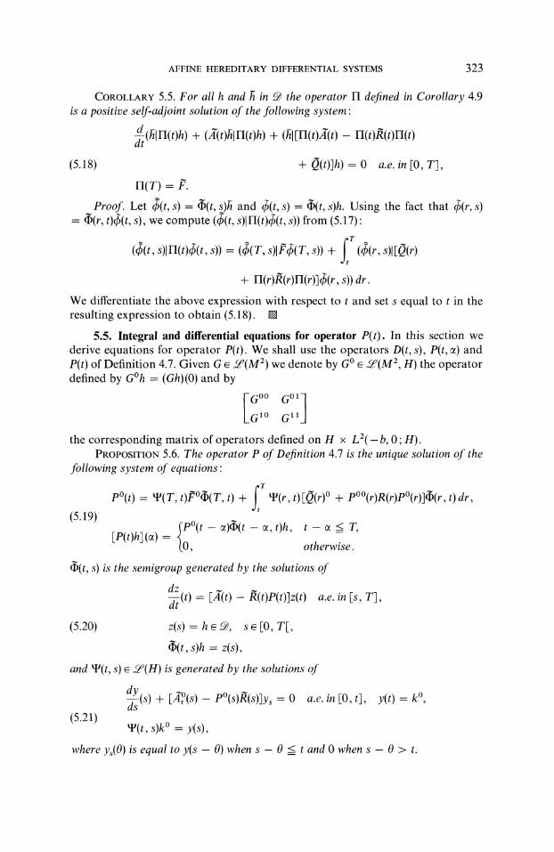
COROLLARY 5.5. For all h and h in the operator H defined in Corollary 4.9is a positive self-adjoint solution of the following system"
d(lH(t)h + ((t)hll-I(t)h) + (hl[H(t)/(t)- H(t).(t)H(t)dt
+ Q(t)]h) 0 a.e. in [0, T],
n(T) F.Proof. Let (t, s) (t, s_)h and (t, s) (t, s)h. Using the fact that (r, s)
(r, t)p(t, s), we compute (t(t, s)ll-I(t)p(t, s)) from (5.17)"
((a(t, s)lFI(t)(t, s)) ((T, s)l(T, s)) + (@r, s)l[0(r)
+ I-I(r)R(r)H(r)]dp(r, s)) dr.
We differentiate the above expression with respect to and set s equal to in theresulting expression to obtain (5.18). k
5.5. Integral and differential equations for operator P(t). In this section wederive equations for operator P(t). We shall use the operators D(t, s), P(t, ) andP(t) of Definition 4.7. Given G 9(M2) we denote by GO 6 (M2, H) the operatordefined by Gh (Gh)(O) and by
G G1GO G
the corresponding matrix of operators defined on H x L2( b, 0;H).PROPOSITION 5.6. The operator P of Definition 4.7 is the unique solution of the
following system of equations"
T
P(t) tP(T, t)ff(T, t) + tP(r, t)[Q(r) + P(r)R(r)P(r)](r, t)dr,
(5.19)fP(t a)(t a, t)h, <= T,
[P(t)h] (a) "{(0, otherwise.
(t, s) is the semigroup generated by the solutions ofdz--(t) [A-(t) (t)P(t)]z(t) a.e. in Is, T],dt
(5.20) z(s) h 9, s [0, T[,
(t, s)h z(s),
and tP(t, s)e (H) is generated by the solutions of
__dY (s) + [/(s) P(s)_(s)]y 0 a.e. in [0, t],ds
(5.21)’e(t, s)k y(s),
where ys(O) is equal to y(s O) when s 0 and 0 when s 0 > t.
y(t) k,
324 M. C. DELFOUR AND S. K. MITTER
(5.22)
Proof. (i) Notice that (5.20) and (5.21) are only functions of P(t). Assume thatP(t) of Definition 4.7 is the unique solution of the first equation of (5.19). We haveshown that
O(r, s) D(r, s)h D(r, r)dp(r, s), r >= s
(Corollary 4.4 and Lemma 4.5). The above equation can be rewritten
D(r, s)h D(r, r)(r, s)h.We let r e and s in the above equation and use Definition 4.7 to obtainthe second equation of (5.19).
(ii) Uniqueness. Let P(t) be a solution of systems (5.19)-(5.21). Let (.,s)be the solution in Is, T] of the following equation"
s) s) Is,.(t)P(t)](t, in
6(s, s) h.
By definition,
(5.23)We define
(5.24)
6(t, s) (t, s)h.
O(t, s) P(t)p(t, s).
We use (5.21) to obtain
(5.25) 0(,)= W(T,t)F4)(T,s)+ tP(r,t)[(r) + P(r)R(r)P(r)])(r,s)dr.
We differentiate with respect to both sides of (5.25)"
ct O(t, s) + gr(t)(t, s) + Q(t)c/)(t, s) 0 in [s, T],(5.26)
0(T, s) Fb(T, s),where (t, s)(O) is equal to 0(t 0, s) when 0 < T and 0 when 0 > T.
We can also rewrite (5.22) using (5.24)"
--qb(t, s) A-(t)(t, s) .(t)(t, s) in Is, T],
(5.27)6(s, s) h.
System (5.26)-(5.27) is the optimality system (4.17)-(4.18) and we know (Lemma4.5 and Definition 4.7) that
(5.28) 0(s, s) P(s)h.Let s in (5.24) and (5.28)"
(5.29) P(s)h /(s, s)= P(s)h.Since this is true for all s e [0, T[, we have established that a solution (if it exists) ofsystem (5.19)-(5.21) is necessarily unique and equal to p0.
(iii) Existence. Let P be as in Definition 4.7. The optimality system (4.17)-(4.18) can be put in the form (5.26)-(5.27) and (5.28) is true by Lemma 4.5 andDefinition 4.7. As a result, (I)(t, s) and tP(t, s) are well-defined and equation (5.26)
AFFINE HEREDITARY DIFFERENTIAL SYSTEMS 325
can be rewritten as follows"
+ [O(t) + P(t)(t)P(t)](t, s)= 0 a.e. in Is, T],
(5.31) O(T, s) Fdp(T, s).
Using (2.22) we can rewrite system (5.30)-(5.31) in integral form"
(5.32) O(t, s) (T, t)Fd(T, s) + (r, t)(0(r) + P(r)/(r)P(r))q(r, s) dr.
By using the relations
(t, s) (t, s)h and P(t)(t, s) 0(t, s),(5.33)
(5.32) becomes
(5.34)[ 5,
T
P(t)(t, s) tP(T, t)FO(t, s) + tP(r, t)(O(r)
+ P(r).(r)P(r))(r, s) dr] h.
Let s in (5.34) and use the fact that (s, s) h to obtain (5.21). This shows thatpO is a solution of system (5.19)-(5.21). []
COROLLARY 5.7. The operators pO and D of Definition 4.7 are solutions of thefollowing coupled system"
D(r, s) P(r)(r, s),(5.35)and for all h,
r>s
d--[P(t)h] + [P(t)(t) + Aoo(t)*P(t)dt
.N A,(t Oi)*D(t 0, t), t- Oi <= T+i=l (0, otherwise J
(5.36) ;o {Ao,(t 00)*D(t-O t)t-O< T/ dO- P(t)R(t)n(t)O, otherwise )
+ Q(t)]h 0 a.e. in 0, T],
po(T fro.
Proof. Consider equation (5.30). Using (5.28) and (5.20) we can compute
(5.37) (t, s) -u[P(u)(t, s)],=t + P(t)[(t) (t)P(t)](t, s).
Let s-- in (5.30) and (5.37). Using the definition of/r and (t, t) we obtain(5.36). k
Remark. P(t) can be obtained from D(r, s) (Definition 4.7)"
[P(t)h](oO= P(t,a)h= D(t- a,t)h, t-o <= T.
326 M. C. DELFOUR AND S. K. MITTER
To complete the picture we need an equation for D. This equation can be formallyobtained provided that the semigroup O(r, s) of system (5.20) is a solution of thefollowing equation"
s)* + a.e. [0, r],(s) (s)P(s)]*7(r, S)* 0 in
(I)(r, r)* I.
This is equivalent to postulating the existence of a topological adjoint system forsystem (5.20). Under this hypothesis we formally differentiate (5.35) with respect tos to obtain the desired differential equation for D"
8 D(r, s) + D(r, s)[(s) ,(s)P(s)] 0 a.e. in [0 r]S
m(r, r) P(r).Let (r,s)= (t- , t) in the above equation. Since P(t, )= D(t- , t) we canobtain the following differential equation for P(t, )"- + P(t, ) + P(t, o0[A(t R(t)P(t)] 0
in the region {(t, ) [0, T] x I(- b, O)]t __< T} with boundary conditions
P(s, O) P(s), s e [O, T].
For completeness we also include the following result which is obtained bydecomposition of (5.17) and the first equation of (5.19).
CoeoLaeY 5.8. Tke operator FI defined in Corollary 4.9 is tke unique solutionof the following system of equations"
H(t) (T, t)F(T, t) + tP(r, t)Q(r)(r, t) dr
(5.38)
+ (r, t)II(r)R(r)[H(r)(r, t) + Hl(r)(r, t)] dr,
1-I(t) (T, t)Fl(T, t) + (r, t)Q(r)(r, t) dr
(5.39)
+ tI(r, t)l-[(r)R(r)[rI(r), (r, t) + n (r) l(r, t)] dr,
(5.40) Hl(t) H l(t)#,T
1-Ill(t) ()l(T t)*Fl(T, t) + (l(r, t)*Q(r)l(r, t)dr
T
(5.41) + j [II(r)(r, t) + rio l(r))l l(r, t)]*R(r)[H(r)g) (r, t)
q- l-[1(r)11(r, t)] dr,
AFFINE HEREDITARY DIFFERENTIAL SYSTEMS 327
where (t, s), defined by (5.16), and W(t, s), defined by (5.21), only depend on I-Iand 1-I 1.
Proof. To derive (5.38) and (5.39) we decompose (5.19) and use the fact thatFl(t) P(t), and to derive (5.41) we decompose (5.17).
Remark. Equation (5.38) relates 1-I to H and 1-11, equation (5.39) relates1-I1 to I-I and 1-I1 and equation (5.41) explicitly relates H 11 to 1-I and H1.
Acknowledgment. It is a pleasure to acknowledge interesting and enlighteningdiscussions we have had with Professor J. L. Lions of the University of Paris.
Notes added in proof1. It can be shown that in Proposition 5.4 and Corollary 5.5 the map
s I-I(s) [0, T] - a(m2) is continuous and for all h, h in @ the map s (hlI-I(s))is in ACI(O, T; R). Somewhat similar remarks can be made for the map t-- P(t)in Proposition 5.6 and Corollary 5.7.
2. The relationship between controllability, stabilizability and the infinitetime quadratic cost problem has been clarified. See:(a) M. C. DELFOUR AND S. K. SITTER, LZ-stability, stabilizability and the infinite
time quadratic cost problem for linear autonomous hereditary differentialsystems, Rep. C.R.M.-132, Centre de Recherches Math6matiques,Universit6 de Montr6al, 1971 submitted to this Journal.
(b) H. F. VANDEVENNE, Qualitative properties of a class of infinite dimensionalsystems, Doctoral thesis, Electrical Engineering Dept., M.I.T., Cam-bridge, Mass., 1972.
3. The following reference which appears to be relevant to the present workwas pointed out to us by the referee:A. MANITIUS, Optimum control of linear time-lag processes with quadratic per-
formance indices, Proc. 4th IFAC Congress, Warsaw, Poland, 1969.
REFERENCES
1] Y. ALEKAL, P. BRUNOVSK, D. H. CHYUNG AND E. B. LEE, The quadratic problemfor systems withtime delay, IEEE Trans. Automatic Control, AC-16 (1971), pp. 673-687.
[2] A. F. BUCKAIO, Explicit conditionsfor controllability oflinear systems with time lag, Ibid., AC-13(1968), pp. 193-195.
I3] D. H. CH’’UNG AND E. B. LE, Linear optimal control problems with time delays, this Journal, 4(1966), pp. 548-575.
[4 G. DA PRATO, Equations d’Ovolution dans des algkbres d’opOrateurs et application d des Oquationsquasi-linOaires, J. Math. Pures Appl., 48 (1969), pp. 59-107.
[5] M. C. DIFOU, Function spaces with a projective limit structure, J. Math. Anal. Appl., to appear.[6] M. C. DIFOUrt AND S. K. MITTR, Hereditary differential systems with constant delays. I--General
case, Centre de Recherches Math6matiques, Universit6 de Montr6al, Canada, 1970" J.Differential Equations, to appear.
I7] ----, Hereditary differential systems with constant delays. II--A class of affine systems and theadjoint problem, Centre de Recherches Math6matiques, Universit6 de Montr6al, Canada,1970; submitted to J. Differential Equations.
[8] --, SystOmes d’Oquations diffOrentielles hOrOditaires retards fixes. ThOorkmes d’existence et
d’unicitk, C. R. Acad. Sci. Paris, 272 (1971), pp. 382-385.[9] , SystOmes d’Oquations diffOrentielles hOrOditaires dl retards fixes. Une classe de systkmes
affines et le problkme du systkme adjoint, Ibid., 272 (1971), pp. 1109-1112.
328 M.C. DELFOUR AND S. K. MITTER
[10] --, Le contrfle optimal des systkmes gouvern6s par des quations diffOrentielles hkrOditairesaffines, Ibid., 272 (1971), pp. 1715-1718.
[11] --, Controllability and observability for infinite-dimensional systems, this Journal, 10 (1972).[12] N. DtNVORD AND J. T. SIaWARTZ, Linear Operators. I, Interscience, New York, 1967.[13] D. H. ELI, J. K. AGGAWAI AYD H. T. BANKS, Optimal control of linear time-delay systems,
IEEE Trans. Automatic Control, AC-14 (1969), pp. 678-687.1-14] H. O. FATVOINI, Some remarks on complete controllability, this Journal, 4 (1966), pp. 686-694.[15] On complete controllability of linear systems, J. Differential Equations, 3 (1967), pp.
391-402.1-161 J. K. HAI, Functional Differential Equations, Springer-Verlag, New York, 1971.
1-17] A. HALANAY, On a boundary-value problem for linear systems with time lag, J. Differential Equa-tions, 2 (1966), pp. 47-56.
[18] On the controllability of linear difference-differential systems, Mathematical SystemsTheory and Economics, II, H. W. Kuhn and G. P. Szeg6, eds., Springer-Verlag, Berlin,1970, pp. 329-335.
[19] D. R. HAIr,Y, R"-Controllability for differential-delay equations, Doctoral thesis, MathematicsDept., University of Maryland, College Park, 1970.
1-201 V. JURDJEVIC, Abstract control systems." Controllability and observability, this Journal, 8 (1970),pp. 424-439.
[211 R. E. KALrAN, Mathematical description of linear dynamical systems, this Journal, (1963),pp. 152-192.
[22] F. M. KIRILLOVA AND S. V. CHURAKOVA, Theproblem ofthe controllability oflinear systems with anafter-effect, Differential Equations, 3 (1967), pp. 221-225.
[231 N. N. KRASOVSKII, On the analytic construction of an optimal control in a system with time lags,Prikl. Mat. Meh., 26 (1962), pp. 39-51 J. Appl. Math. Mech., 26 (1962), pp. 50-67.
1-241 --, Optimal processes in systems with time lags, Proc. 2nd IFAC Conf., Basel, Switzerland,1963.
25] H. J. KusrINZ AND D. I. BARNA, On the control of a linear functional-differential equation withquadratic cost, this Journal, 8 (1970), pp. 257-272.
[26] J. L. LIONS, Contr6le optimal de systkmes gouvernOs par des Oquations aux dOrivkes partielles,Dunod, Paris, 1968; English transl., Springer-Verlag, Berlin, New York, 1971.
E271 D. L. LtKzs AND D. L. RtSSLI, The quadratic criterion for distributed systems, this Journal,7 (1969), pp. 101-121.
[28] S. K. MITTER, Optimal control of distributed parameter systems, Joint Automatic Control Con-ference (Boulder, Colo., 1969), ASME, New York, 1969, pp. 13-48.
[29] V. M. PoPov, Private communication.[30] D. W. Ross AND I. FL/0GG-Loa’z, An optimal control problem for systems with differential-differ-
ence equation dynamics, this Journal, 7 (1969), pp. 609-623.
[31] L. M. SILVERMAN AND H. E. MZADOWS, Controllability and observability in time-variable linearsystems, this Journal, 5 (1967), pp. 64-73.
[32] G. S. TAHIM, Controllability of linear systems with time lag, Proc. 3rd Allerton Conf. on Circuit
and System Theory, Urbana, Ill., 1965, pp. 346-353.
[33] L. WIss, On the controllability of delay-differential systems, this Journal, 5 (1967), pp. 575-587.
[34] --, An algebraic criterion for controllability of linear systems with time delay, IEEE Trans.Automatic Control, AC-15 (1970), pp. 443-444.
[35] ----, New aspects and results in the theory of controllability Jbr various system models, JointAutomatic Control Conference (Boulder, Colo., 1969), ASME, New York, 1969, pp.453-456.
[361 Lectures on controllability and observability, C.I.M.E. Seminar on Controllability andObservability, Edizioni Cremonese, Rome, 1969, pp. 205-289.
[37] W. M. WONrA, On a matrix Riccati equation of stochastic control, this Journal, 6 (1968), pp.681-697.
Related Documents


![RESEARCH REPORT-2013-08-21 30–1 On the Controllability and ... · arXiv:1401.4335v1 [cs.SY] 17 Jan 2014 RESEARCH REPORT-2013-08-21 30–1 On the Controllability and Observability](https://static.cupdf.com/doc/110x72/5fc991f91964ed6233533cb3/research-report-2013-08-21-30a1-on-the-controllability-and-arxiv14014335v1.jpg)

