Numerical Aspects and Implementation of
Population Balance Equations Coupled with Turbulent Fluid
Dynamics
E. Bayraktar∗, O. Mierka, F. Platte, D. Kuzmin and S. Turek
Institute of Applied Mathematics (LS III), University of DortmundVogelpothsweg 87, D-44227, Dortmund, Germany.
E-mail: [email protected]
Abstract
In this paper, we present numerical techniques for one-way coupling of CFD and Popu-lation Balance Equations (PBE) based on the incompressible flow solver FeatFlow whichis extended with Chien’s Low-Reynolds number k − ε turbulence model, and breakage andcoalescence closures. The presented implementation ensures strictly conservative treatmentof sink and source terms which is enforced even for geometric discretization of the internalcoordinate. The validation of our implementation which covers wide range of computa-tional and experimental problems enables us to proceed into three-dimensional applicationsas, turbulent flows in a pipe and through a static mixer. The aim of this paper is to high-light the influence of different formulations of the novel theoretical breakage and coalescencemodels on the equilibrium distribution of population, and to propose an implementationstrategy for three-dimensional one-way coupled CFD-PBE model.
1. Introduction
Population balances may be regarded either as an old subject that has its origin in theBoltzmann equation more than a century ago, or as a relatively new one in light of thevariety of applications in which engineers have recently put population balances to use.Population balance equations (PBE) are essential to researchers of many distinct areas.Applications cover a wide range of dispersed systems, such as solid-liquid (crystallizationsystems), gas-solid, gas-liquid (aerobic fermentation) and liquid-liquid (food processes)dispersions. Analysis of separation and reactor equipments and dispersed phase reactors,they all involve population balance models [40].
In practical applications, a single bubble size model, as reported by numerous re-searchers [36, 22], cannot properly describe the interfacial interactions between the phases,and analytical solutions of the PBE are available just for very few and specific cases.Hence, the use of appropriate numerical techniques is unavoidable in order to deal withpractical problems. There are several numerical methods satisfying the necessary require-ments with respect to robustness and realizability: the quadrature method of moments[34, 33], the direct quadrature method of moments (DQMM) [10], parallel parent anddaughter classes (PPDC) [4] and the method of classes [18, 19], which is in the scope of
1

this study.
In the literature, there are several noticeable breakup and coalescence models. Thesetwo competing mechanisms for static conditions finally lead the distribution to a certaindynamic equilibrium. Thus, it is important to have compatible kernels for coalescence andbreakage. If one of these kernels is dominant with respect to the other, the achievementof an equilibrium distribution can be unrealistic. Therefore, the breakage and coalescencekernels are usually modeled together. Chen and his co-workers [6] studied the effect ofdifferent breakage and coalescence closures and they showed that incompatible kernelsproduce poor results. Certain experimental and theoretical models for breakage andcoalescence kernels are regarded as milestones for the evolution of population balancesin the framework of liquid/gas-liquid dispersed phase systems and the evolution of thesemodels is presented in detail by [15].
Most of the present models for coalescence kernels were derived analogously to kinetictheory of gases [9, 45, 39, 30]. In kinetic theory of gases, collisions between moleculesare considered while in the process of coalescence, bubble (droplet)–bubble (droplet) andbubble/droplet–eddy collisions count. Thus, various coalescence models show similartrends, that is a monotonous increase in the specific coalescence rate with increase inthe bubble/droplet diameter [5]. The coalescence kernel function adopted in this workis the one proposed by Lehr et al. [28] which is implemented according to the techniquedeveloped by Buwa and Ranade [5].
In the case of breakup, most of the published studies on bubble/droplet breakup arederived from the theories which are outlined by [12] and [16]. All these models have theirown advantages and weak points which makes them dramatically different. Nevertheless,they have similar phenomenological interpretations: bubble/droplet breakage occurs dueto turbulent eddies colliding with the bubble/droplet surface. If the energy of the incom-ing eddy is higher than the surface energy, deformation of the surface happens, which mayresult in breakup of a bubble/droplet into two or more daughter bubbles/droplets. Thecolliding eddies that are larger than the bubble/droplet result in spatial transportation.Thus, collisions between bubble/droplet and eddies which are smaller than or equal insize to the bubble/droplet, give rise to breakage. The main differences among the avail-able models are due to their predictions of daughter size distributions (DSD). Some ofthe models assume a uniform or a truncated normal distribution which is centered at thehalf of the bubble/droplet size. In other words these models are based on the assumptionof equal-sized breakage [2, 26, 47]. In contrast, some others presume unequal breakupwhich means a bubble/droplet breaking into a large and a smaller one [2, 31, 45]. Thedeveloped model by [27] is able to combine the features of these significantly differentbreakage closures. Their model is based on the theoretical findings of [31]. The breakagekernel is derived from the frequency of arriving eddies onto the surface of a bubble andfrom the probability that collisions lead to breakage. Accordingly, their model predicts anequal-sized breakage for relatively small bubbles/droplets and an unequal-sized breakagefor large ones. In fact, their approach appears even intuitively to be reasonable: large
2

bubbles/droplets firstly collide with large turbulent eddies so that a large and smallerdaughter bubble/droplet exists while for small bubbles/droplets equal-sized breakage iseasier due to high interfacial forces (large and small are relative to stable bubble sizeunder given conditions). A comprehensive comparison of the noticeable coalescence andbreakage models is given by [48]. The comparison shows that the model proposed by[28] is generally superior to other available breakup closures which makes it a suitablecandidate for the choice of our breakage kernels.
There are many hydrodynamic variables which affect the efficiency of multiphase reac-tors. However, one should be able to resolve the flow field in the reactor in order to calcu-late the necessary breakup and coalescence kernels to solve the population balance equa-tions, that means to solve the transport problems in the internal (size of drops/bubbles)and external (spatial) coordinates. This attempt will involve an inevitable coupling be-tween CFD and PBE which can lead to irrational computational cost and many difficultiesin numerics if the problem is not tackled properly.
The dynamics of gas/liquid-liquid dispersed flows has been a topic of research for thelast several decades and many different methods were developed. Numerical simulation offlow fields in column reactors, which is a cumbersome problem due to high complexity ofthe flow field, is possible by adopting the Euler-Euler or Euler-Lagrange approaches. Forpractical reasons like high numerical efforts and computational costs which are related totracking and calculating the motion of each bubble individually in the flow field, the for-mer method is restricted to be applied on lean dispersions or when low volume fractions ofthe dispersed phase are considered, while the latter method requires comparatively smallefforts in both numerics and computation. Nevertheless, both of the methods lead to thesame results if the problems are handled with adequate computational effort as it hasbeen reported by [44]. Sokolichin and Eigenberger went on with their studies and theyelucidated the behavior of flow fields in bubble columns. Numerical simulations whichassume the flow to be laminar are not able to produce mesh independent results. The finerthe grid, the more vortices are resolved. That is more typical for turbulent flows. Hence,they performed extensive numerical calculations and conducted several experiments afterwhich they concluded that turbulence models are more convenient to describe flow fieldsin bubble columns [3, 43].
Turbulence models which are applicable to produce results with an acceptable accuracyand reasonable computational cost in general originate from the family of two-equationeddy viscosity models. The most preferred model in this sense is related to the standardor modified k-ε turbulence model which has been implemented in several commercialCFD programs and in-house codes. In most of the present studies which consider im-plementation of CFD coupled with PBE, it is preferred to work with commercial codeslike FLUENT [1, 6, 32, 38] or CFX [5, 7, 28, 27], naming just two of the most importantCFD software packages. However, a commercial code is not the only option and open-source software packages such as FeatFlow (see http://www.featflow.de) extended with
3
additional modules (such as turbulence model [20], multiphase model [22], subgrid-scalemixing model [35] or a population balance model in the present case) possess the advan-tages of higher flexibility and robustness.
The paper is organized as follows. In Section 2 the mathematical model of the popula-tion balance equation with the breakage and coalescence kernels is described. In Section 3,the arising standalone implementation of the obtained mathematical model is dealt with.Furthermore, the description of its integration into the CFD flow solver is given in Section4. The validation of our implementation together with the CFD coupled applications formthe content of Section 5, which is followed by our conclusions.
2. Mathematical model
The population balance equation for gas-liquid (liquid-liquid) flows is a transport equationfor the number density probability function, f , of bubbles (drops). By definition, f needsto be related to an internal coordinate, what in most of the cases is the volume of bubbles,υ. Therefore, the number density, N , and void fraction, α, of bubbles having a volumebetween υa and υb are:
Nab =
∫ υb
υa
f dυ, αab =
∫ υb
υa
fυ dυ. (1)
The considered transport phenomena account for convection in the physical space (gov-erned by the flow field ug), while the bubble breakage and coalescence move the bubblesin the space of the internal coordinate. Thus, the resulting transport equation is thefollowing
∂f
∂t+ ug · ∇f = B+ + B− + C+ + C−. (2)
Clearly, in case of modeling turbulent flows according to (temporal) averaging concepts(2) has to be extended by the arising pseudo diffusion terms in analogy to the approachof the Reynolds stress tensor
∇ · u′f ′ = −∇ · (νTσT
∇f), (3)
where σT is the so-called turbulent Schmidt number. In (2) the superscripts ”+” and ”–”stand for sources and sinks and the terms B and C on the right hand side represent therate of change of the number density probability function,
(
dfdt
)
, due to bubble breakupand coalescence, respectively. In this study, both of these processes are modelled inaccordance with the two most popular models of Lehr and his colleagues [27, 28] adoptingsome modifications with respect to an implementation introduced by [5]. According tothese studies:
• the breakage of parent bubbles of volume υ into bubbles of volume υ and bubblesof volume υ − υ is associated with a rate rB(υ, υ)f(υ),
4

• the coalescence of parent bubbles of volume υ with bubbles of volume υ− υ formingbubbles of volume υ is associated with a rate rC(υ − υ, υ)f(υ)f(υ − υ),
where rB and rC are the so called kernel functions of breakup and coalescence. Substi-tution of the breakage and coalescence terms into (2) results in the following transportequation
∂f
∂t+ ug · ∇f =
∫
∞
υ
rB(υ, υ)f(υ) dυ − f(υ)
υ
∫ υ
0
υrB(υ, υ) dυ
+1
2
∫ υ
0
rC(υ, υ − υ)f(υ)f(υ − υ) dυ − f(υ)
∫
∞
0
rC(υ, υ)f(υ) dυ,
(4)
which still needs to be closed by the specification of the kernel functions rB and rC .According to [27] the coalescence kernel function is defined by
rC(υ, υ) =π
4(d+ d)2min(u′, ucrit), (5)
with d and d denoting the diameter of bubbles of υ and υ. The characteristic velocitiesu′ and ucrit are computed as follows
u′ =√2ε1/3(dd)1/6, (6)
ucrit =
√
Wecritσ
ρldeqwith deq = 2(d−1 + d−1)−1, (7)
where ε is the turbulent dissipation rate, σ is the surface tension of the liquid phase, ρlis the density of the liquid phase, and Wecrit is the critical Weber number being equal to0.06 for pure liquids [28]. Alternatively, it is also common to assume u′=0.08m/s insteadof considering u′ to be a function of υ and υ as it was done in the study of Lehr andhis colleagues [28]. However, under certain conditions this assumption seems to lead tounphysical results which are shown and explained in the following section. Additionally,the chosen coalescence kernel (5) shows similar trends (monotonous increase in the specificcoalescence rate with increase in bubble diameter) in relation to experimental observationsand as most of the other models in the literature [5].
Regarding the breakup kernel there are various different formulations which yieldsignificantly different results. For that reason, it is hard to say that one model canhighlight all the features of the given process. A comparison of the most remarkablebreakup kernels in the literature is carried out by [48]. In pursuit of the mentioned studyit is shown that the model presented by [28] is more comprehensive than any other modelin the literature. The model in question [28] is based on the practical formulation of thetheoretical findings reported by [31] which therefore forms the fundamental basis of manyother relevant breakage models.
Motivated by the wide diversity of available breakage models presented in the litera-ture, we extended our scope by consideration of a second breakage model developed by
5

0 0.2 0.4 0.6 0.8 10
2
4
6
8
10
fBV
DS
D
v=1.25v*v=2.5v*v=10v*
Figure 1: Dimensionless daughter size distribution.
[27]. This model also originates from the pioneering theoretical formulation introducedby [31], that enables us to compare the same theoretical model from the point of viewof two different practical interpretations. Additionally, both of the breakage models havethe following definition in common
rB(υ, υ) = KBΦ(υ, υ), (8)
where KB is the total breakage rate and Φ(υ, υ) is the probability of breaking bubbles ofvolume υ into bubbles of volume υ. The choice of our first breakage closure was influencedby the demonstrated excellent properties of the breakage kernel developed by [27]. As aresult of this work, the total breakage rate KB is defined as
KB = 1.5(1− αg)(ρlσ
)2.2
ε1.8. (9)
The aforementioned excellent properties of the adopted breakage kernel are hidden in thedefinition of the daughter size probability distribution function φ(υ, υ), which naturallyprovides equal and unequal size distributions for the daughter bubbles (see Fig. 1). Sucha behavior of the distribution function is achieved by the following formula
φ(υ, υ) = max
(
ω1/3
ω4/3
(
min(
ω7/6, ω−7/9)
− ω−7/9)
, 0
)
forω
ω∈ (0, 0.5〉
with ω = υπ
6
σ1.8
ρ1.8l ε1.2and ω = υ
π
6
σ1.8
ρ1.8l ε1.2.
(10)
According to the implementation technique developed by [5], the substitution of the di-mensionless bubble volume fBV = ω
ω= υ
υinto (10) results in
φ(υ, υ) = max(
ω−1f−4/3BV
(
min(
(fBV ω)7/6 , (fBV ω)
−7/9)
− ω−7/9)
, 0)
for fBV ∈ (0, 0.5) ,(11)
6

and makes it possible to analytically integrate the DSD in arbitrary limits. Being consis-tent with the assumption that the breakup process results in a pair of daughter bubblesof volume υ and υ − υ, this requires symmetry of the function φ(υ, υ) = φ(υ, υ − υ) forfBV ∈ (0.5, 1) (see Fig. 1). Finally, the mean probability of breaking a bubble of volumeυ into a bubble between (υ −∆υ) and (υ +∆υ) can be obtained as follows
Φ(υ, υ) =υ
2∆υ
∫ υ+∆υυ
υ−∆υυ
φ(υ, υ) dfBV . (12)
The second adopted breakage kernel is the one proposed by [28]. Both, the total breakagerate KB and the breakage probability Φ(υ, υ) are defined as a function of the followingtime and length scales
T =
(
σ
ρL
)0.61
ε0.4and L =
(
σ
ρL
)0.41
ε0.6. (13)
Introducing the dimensionless bubble diameter d∗ = d/L and bubble volume υ∗ = υ/L3
gives rise to:
KB =d∗5/3
2Texp
(
−√2
d∗3
)
(14)
φ(υ, υ) =6
(
L√πd∗)3
exp
(
−2.25(
ln(
22/5d∗))2
)
1 + erf(
ln (21/15d∗)1.5) for υ∗ ∈ (0, 0.5〉 (15)
and φ(υ, υ) = φ(υ, υ − υ) for υ∗ ∈ (0.5, 1) (16)
The phenomenological models involve several parameters in their formulations which arestrictly depending on the operating conditions and the system. Thus, they are specificto the problem as in the study of [45], whereas in theoretical models formulations donot consist of these empirical parameters; therefore they are supposed to be applicablein a wide range of operating conditions. The explained theoretical breakage closures arechosen due to their applicability in a broad range of operating conditions and similaritiesin the outline of their formulations, and to show how the peculiarities of these modelsinfluence the results of numerical simulations in the validation process.
3. Implementation of PBE
In this study, the discretization of the population balance equation (4) is carried outby the method of classes (with piecewise constant approximation functions). The fixedpivot volume of the classes is initialized by specifying the bubble volume of the smallest”resolved” class υmin and the discretization factor q, such that
υi = υminqi−1 with i = 1, 2, ...n (17)
7
where n is the number of classes. The class width ∆υi is defined by the difference of theupper υU
i and lower υLi limit of the given class i:
∆υi = υUi − υL
i with υUi = υL
i+1 and υUi−1 = υL
i . (18)
The limits are fixed and initialized such that in the case of q = 2 the pivot volume υi iscentered in the class
υUi = υi +
1
3(υi+1 − υi), υL
i = υi −2
3(υi − υi−1). (19)
The discretized transport equation (4) of the i-th class’ number density probability, fi,results in
∂fi∂t
+ ug · ∇fi =n∑
j=i
rBi,jfj∆υj −fiυi
i∑
j=1
υjrBj,i∆υj
+1
2
i∑
j=1
rCj,kfjfk∆υj − fi
n∑
j=1
rCj,ifj∆υj for i = 1, 2, ...n.
(20)
The choice of fixed bubble pivot volumes and fixed class widths offers the advantage ofexpressing the discretized transport equation (20) in terms of class holdups αi insteadof the number probability density, fi = αi
υi∆υi(see (1)). Doing so enforces only mass
conservation, however the bubble number density may not be conservative. Regarding thearising inconsistency we subscribe to the argument of [5], who reported that the differencein the predicted values of interfacial area and Sauter mean bubble diameter obtainedwith only mass conservation and obtained with mass and bubble number conservationwas less than 1%. Multiplying equation (20) with υi∆υi results in conservative sourceand sink terms, since the overall gas-holdup cannot be changed due to coalescence orbreakup procedures
1
. Additionally, any sink (source) term of a given rate associated to aparticular breakup or coalescence procedure induces a source (sink) term with the samerate but in a different class. This enables us to assemble only the sink terms while thesame contribution is applied to the corresponding source term in the resulting class. Letus for example consider a breakup of bubbles of class i into bubbles of classes j and k.Such a procedure will result in the following right hand sides
i : −(
υjrBi,j∆υj
fiυi
)
υi∆υi −(
υkrBi,k∆υk
fiυi
)
υi∆υi = −rBi,jαiυj∆υj
υi−rBi,kαi
υk∆υkυi
j : +(
υjrBi,jfi∆υi
)
υj∆υj = rBi,jαiυj∆υj
υi
k : +(
υkrBi,kfi∆υi
)
υk∆υk = rBi,kαiυk∆υk
υi∑
= 0
where υk = υi − υj.
However, if we consider the coalescence of bubbles/droplets of the j’th and the k’thclass to form bubbles/droplets of the i’th class, to show the conservation of void fraction
8

is a little bit more tricky. The losses in the k’th and j’th classes due to coalescence witheach other are as follows:
j : −(
fjrCj,kfk∆υk
)
υj∆υj = −rCj,kαjfk∆υkk : −
(
fkrCk,jfj∆υj
)
υk∆υk = −rCk,jαkfj∆υj
The gain in the i’th class due to coalescence of the k’th and j’th classes is:
i : 12
(
rCj,kfjfk∆υj + rCk,jfkfj∆υk)
υi∆υi
If we assume that the discretization is equidistant, that means ∆υi = ∆υj = ∆υk, andrecalling that υi = υj + υk then the following relation is obtained
1
2
(
rCj,kfjfk∆υj + rCk,jfkfj∆υk)
(υj + υk)∆υi = rCj,kαjfk∆υk + rCk,jαkfj∆υj
which shows that the sink and source terms of coalescence are also conservative in termsof void fraction. In this study, geometric grids (for the internal coordinate) with varyingdiscretization constants are employed. Therefore, instead of calculating individual sinkand source terms due to coalescence, only sink terms for each possible pair of classes arecalculated and their sum is added to the resultant bubble class. Accordingly, conservationof mass is enforced from the point of view of coalescence, too.
4. Integration of PBE into CFD
Before proceeding to the description of the developed numerical algorithm, let us recall theproblems related to the integration of PBE into a CFD solver. The main problem whichhas to be clarified at the very first place is based on the identification of the coupling effectsbetween the individual parts of the model (see Fig. 2). Besides the internal coupling of theNavier-Stokes equation (C1 and C2) in case of turbulent flow simulations supported bytwo-equation eddy viscosity models such as k − ε models, additional coupling has also tobe taken into account (C5). At the same time, as a consequence of multiphase modeling,one has to be aware of even more complex coupling effects due to buoyancy (C7) andenhanced turbulence effects (C8). Furthermore, the turbulence and the multiphase modelis coupled by means of the flow field with the Navier-Stokes equation (C5 and C7). Lastbut not least, internal coupling takes place in all the three subproblems (C1, C3 and C4)resulting in a rather interlocking structure. To cope appropriately with the describedstrongly coupled system is quite challenging, and may result in unavoidably increasedcomputational cost. Therefore, in this work the coupling effects are relaxed by not takinginto account the influence of the turbulence induced by the secondary phase (also known asbubble induced turbulence in gas-liquid systems) and by neglecting the buoyancy forces.Accordingly, the description of a one-way coupled implementation follows which is validfor a) pressure driven and b) shear induced turbulence dominating systems.
9

Figure 2: Sketch of the coupling effects inside the complete model.
In this work the motion of fluid flow is governed by the Reynolds Averaged Navier Stokes(RANS) equations of the following form
∂u
∂t+ u · ∇u = −∇p+∇ ·
(
(ν + νT )[∇u+∇uT ])
,
∇ · u = 0,(21)
where ν depends only on the physical properties of the fluid, while νT (turbulent eddyviscosity) is supposed to emulate the effects of the unresolved velocity fluctuations u′.According to Chien’s Low-Reynolds Number modification of the k − ε model the eddyviscosity has the following definition
νT = Cµfµk2
εwith ε = ε− 2ν
k
y2, (22)
where k is the turbulent kinetic energy, ε is the dissipation rate and y is the closestdistance to the wall[8]. Clearly enough, for computations of k and ε the above PDEsystem is to be complemented by two additional mutually coupled convection-diffusion-reaction equations [25]. For our purposes, it is worthwhile to introduce a linearizationparameter γ = τ−1
T = ε/k, which is related to the turbulent time scale τT and whichmakes it possible to decouple the transport equations as follows [29]
∂k
∂t+∇ ·
(
ku− νTσk
∇k
)
+ αk = Pk, (23)
∂ε
∂t+∇ ·
(
εu− νTσε
∇ε
)
+ βε = γC1f1Pk. (24)
The involved coefficients in (23–24) are given by
α = γ +2ν
y2, β = C2f2γ +
2ν
y2exp(−0.5y+), Pk =
νT2|∇u+∇uT |2,
fµ = 1− exp(−0.0115y+), f1 = 1, f2 = 1− 0.22 exp−(
k2
6νε
)2
.
(25)
10

The discretization in space is performed by a finite element method on unstructuredgrids. The incompressible Navier-Stokes equations are discretized using the nonconform-ing Q1/Q0 element pair, whereas standard Q1 elements are employed for k and ε. After animplicit time discretization by the Crank-Nicolson, Fractional-step θ scheme or BackwardEuler method, the nodal values of (v, p) and (k, ε) are updated in a segregated fashionwithin an outer iteration loop.
For n=1,2,... main time-stepping loop tn −→ tn+1
For k=1,2,... outermost coupling loop
• Solve the incompressible Navier-Stokes equations
For l=1,2,... coupling of v and p
For m=1,2,... flux/defect correction
• Solve the transport equations of the k − ε model
For l=1,2,... coupling of k and ε
For m=1,2,... flux/defect correction
• Solve the population balance equation
For l=1,2,... coupling of αi for i = 1, ..., s
For m=1,2,... flux/defect correction
Figure 3: Developed computational algorithm consisting of nested iteration loops.
The iterative solution process is based on the hierarchy of nested loops according to theapproach described in [22] and is presented in Fig. 3. At each time step (one n−loop step),the governing equations are solved repeatedly within the outer k-loop which contains thetwo subordinate l-loops responsible for the coupling of variables within the correspondingsubproblem. The embedded m-loops correspond to iterative flux/defect correction for theinvolved convection-diffusion operators. In the case of an implicit time discretization,subproblem (23–24) leads to a sequence of algebraic systems of the form [21, 23, 46]
A(u(k), γ(l), ν(k)T )∆u(m+1) = r(m),
u(m+1) = u(m) + ω∆u(m+1),(26)
where r(m) is the defect vector and the superscripts refer to the loop in which the cor-responding variable is updated. Flux limiters of TVD type are activated in the vicinityof steep gradients, where nonlinear artificial diffusion is required to suppress nonphysical
11

undershoots and overshoots. The predicted values k(l+1) and ε(l+1) are used to recomputethe linearization parameter γ(l+1) for the next outer iteration (if any). The associatededdy viscosity νT is bounded from below by a certain fraction of the laminar viscosity0 < νmin ≤ ν and from above by νT,max = lmax
√k, where lmax is the maximum admissible
mixing length (the size of the largest eddies, e.g., the width of the domain). Specifically,we define the limited mixing length l∗ as
l∗ =
{
Cµfµk3/2
εif Cµfµk
3/2 < εlmax
lmax otherwise(27)
and calculate the turbulent eddy viscosity νT from the formula
νT = max{νmin, l∗√k}. (28)
The resulting value of νT is used to update the linearization parameter
γ = τ−1T = Cµfµ
k
νT. (29)
The above representation of νT and γ makes it possible to preclude division by zero and toobtain bounded nonnegative coefficients (required by physical reasons and computationalstability) without manipulating the actual values of k and ε.
In the following, remarks concerning the treatment of the convection and sink termsin the population balance equation will be given from the point of view of positivitypreservation. Since the continuous transport equation (4) is positivity preserving for non-negative initial and boundary conditions the same property needs to be satisfied by itsdiscrete counterpart (20). This can be achieved by an implicit treatment of the sink termsresulting in the following set of equations
(
ML +(
θK −B−
i − C−
i
)
∆t)
α(n+1)i,(k+1) = (ML − (1− θ)K∆t)α
(n+1)i,0 + (B+
i + C+i )∆tα
(n+1)i,(k)
where α(n+1)i,0 = αn
i for i = 1, 2, ...n,
(30)
with ML being the lumped mass matrix, K the discretized convection operator, B and Cthe discretized breakage and coalescence terms. In case of an implicit time discretization,such as Crank Nicolson or Fractional-step θ time stepping, subproblem (30) leads to thealgebraic system of the form [21, 23, 46]
A(u(n), ν(n)T , B
±(l)i , C
±(l)i )∆α
(m+1)i = r(m),
α(m+1)i = α
(m)i + ω∆α
(m+1)i ,
(31)
where r(m) is the defect vector and the superscripts refer to the loop in which the corre-sponding variable is updated (see the algorithm in Fig. 3).
12
5. Numerical examples
The numerical calculations in scope of this study will be classified into two subsections.The content of the first subsection presents the validation problems, which are supportedby experimental and computational results available in the literature. The content of thesecond subsection deals with a detailed study which couples PBE and CFD in case of aturbulent pipe flow which involves two immiscible fluids.
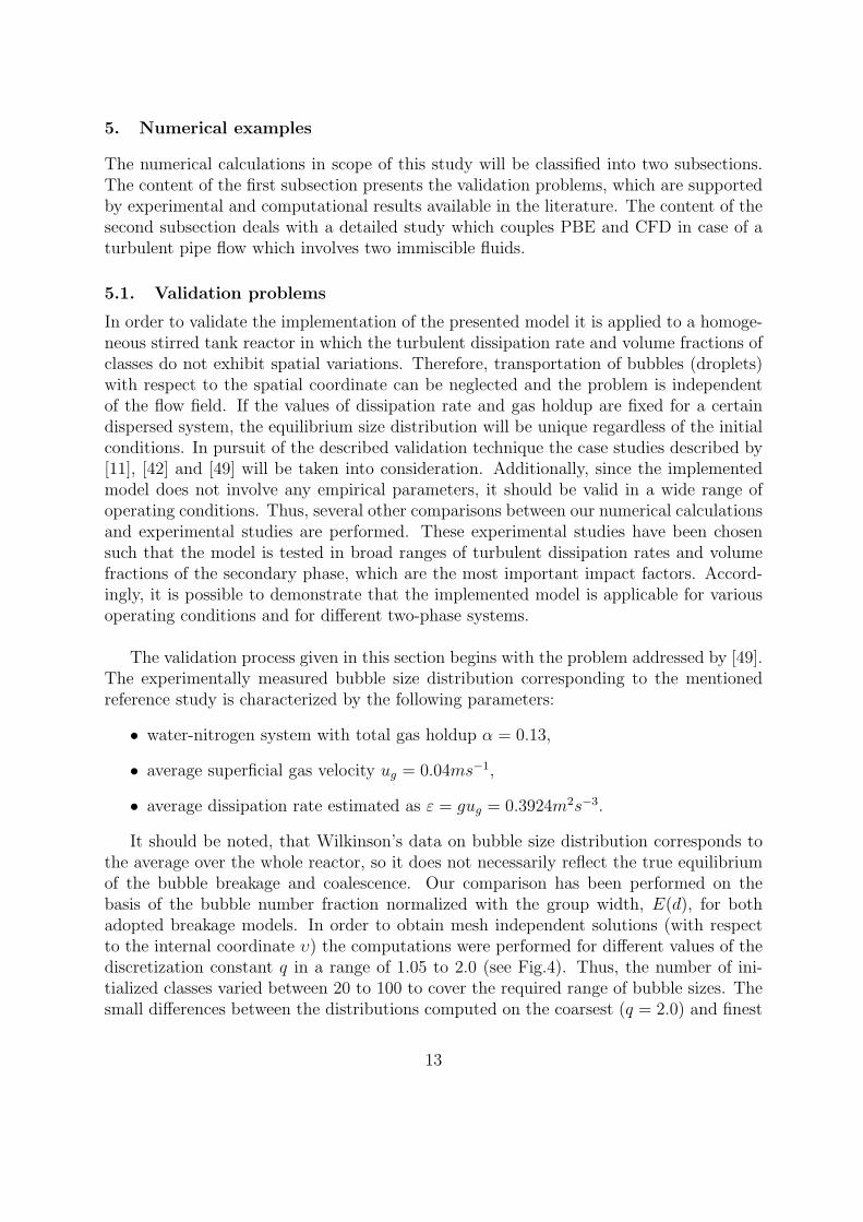
5.1. Validation problems
In order to validate the implementation of the presented model it is applied to a homoge-neous stirred tank reactor in which the turbulent dissipation rate and volume fractions ofclasses do not exhibit spatial variations. Therefore, transportation of bubbles (droplets)with respect to the spatial coordinate can be neglected and the problem is independentof the flow field. If the values of dissipation rate and gas holdup are fixed for a certaindispersed system, the equilibrium size distribution will be unique regardless of the initialconditions. In pursuit of the described validation technique the case studies described by[11], [42] and [49] will be taken into consideration. Additionally, since the implementedmodel does not involve any empirical parameters, it should be valid in a wide range ofoperating conditions. Thus, several other comparisons between our numerical calculationsand experimental studies are performed. These experimental studies have been chosensuch that the model is tested in broad ranges of turbulent dissipation rates and volumefractions of the secondary phase, which are the most important impact factors. Accord-ingly, it is possible to demonstrate that the implemented model is applicable for variousoperating conditions and for different two-phase systems.
The validation process given in this section begins with the problem addressed by [49].The experimentally measured bubble size distribution corresponding to the mentionedreference study is characterized by the following parameters:
• water-nitrogen system with total gas holdup α = 0.13,
• average superficial gas velocity ug = 0.04ms−1,
• average dissipation rate estimated as ε = gug = 0.3924m2s−3.
It should be noted, that Wilkinson’s data on bubble size distribution corresponds tothe average over the whole reactor, so it does not necessarily reflect the true equilibriumof the bubble breakage and coalescence. Our comparison has been performed on thebasis of the bubble number fraction normalized with the group width, E(d), for bothadopted breakage models. In order to obtain mesh independent solutions (with respectto the internal coordinate υ) the computations were performed for different values of thediscretization constant q in a range of 1.05 to 2.0 (see Fig.4). Thus, the number of ini-tialized classes varied between 20 to 100 to cover the required range of bubble sizes. Thesmall differences between the distributions computed on the coarsest (q = 2.0) and finest
13

(q = 1.05) mesh leads us to the conclusion that qualitatively good results can alreadybe obtained by means of coarse grid computations. As it can be seen from Fig. 5, ourcomputational predictions are in a good agreement with the experimental results of [49]and correlate well with the computational results obtained by [5] (especially in the caseof the breakage kernel of [27]) for the same problem and for the same model.
We recall that, in order to obtain the equilibrium between bubble breakup and coales-cence for the population balance equation, one might reduce the original system of PDE’sto a system of ODE’s (neglecting the spatial variation). Then, the steady state solutionof such a reduced (0-dimensional) system (stirred tank reactor model) corresponds to therequired equilibrium distribution. In Fig. 6, experimentally measured data of this type[11, 42] are presented and compared to our computational predictions. The experimentswere conducted with air-water multiphase flow for different volume fractions, α1 = 0.2and α2 = 0.08, and for the same value of superficial gas velocities jg1 = 0.08ms−1 andjg2 = 0.02ms−1 which corresponds to dissipation rates of 0.785m2s−3 and 0.196m2s−3,respectively. The representative quality of the results was chosen to be the “normalized
Figure 4: Steady state bubble size distribution for α = 0.13 and ε = 0.3924m2s−3. Right:Breakage kernel [28]. Left: Breakage kernel [27].
Figure 5: Steady state bubble size distribution for α = 0.13 and ε = 0.3924m2s−3.Comparison of our mesh independent solution with reference data ([49] – experimental,[5] – computational). Right: Breakage kernel [28]. Left: Breakage kernel [27].
14

Figure 6: Computed equilibrium distribution for the breakage models versus experimen-tally measured distribution [11, 42]. Experiment A: α = 0.2 and ε = 0.785m2s−3. Ex-periment B: α = 0.08 and ε = 0.196m2s−3. Right: Breakage kernel [28]. Left: Breakagekernel [27].
number of bubbles per fraction width“, E(d). We obtained a good agreement between theresults of our numerical calculations and the presented experimental results (see Fig. 6).This comparison leads us to conclude that the model by [28] is a more suitable candidatefor implementation into our CFD code.
Before progressing to couple PBE with CFD, it is necessary to verify our implementa-tion for high and low turbulent dissipation rates. Thus, two more studies are examined:the first example has been taken from the study by [24] for high dissipation rate values,and the latter one has been taken from the study of Olmos and his colleagues [37] for lowvalues of dissipation rate.
In the first study, the local bubble size distributions (BSDs) had been measured/modelledfor dense air–water and CO2–n-butanol dispersions under hydrodynamic conditions char-acterized by high turbulent dissipation rates. The experimental [13] and simulation resultsobtained in the reference study of [24] together with our simulation results correspondingto simulation time of 50s are summarized in Tab. 1.
Table 1: Sauter mean diameters (mm)
Case Hu et al. Laakkonen et al. Our study
air-water 0.447 0.359 0.358air-1-propanol 0.316 0.207 0.205air-diethylene glycol 0.598 0.251 0.250
The results are in good agreement with the reference study, in fact they are almost iden-tical. Nevertheless, some remarks are in order. The obtained equilibrium BSDs and theSauter mean diameters are strongly dependent on the stopping criteria of the iterativescheme. This means that the final Sauter mean diameters may slightly change by varying
15

the convergence criteria for resulting in different simulation times (stringent criterion –longer simulation and vice versa). Accordingly, the graphs plotted in Fig. 7 show theevolution of the Sauter mean diameter for two different time intervals.
a)0 10 20 30 40 50
0
0.5
1
1.5
2
2.5x 10
−4
time [sec]
d 32 [m
]
b)0 100 200 300 400 500
0
0.5
1
1.5
2
2.5x 10
−4
time [sec]
d 32 [m
]
Figure 7: Case: air-1-propanol a) for 50 seconds b) 500 seconds
In Fig. 7(a), the convergence criteria – defined as the maximum relative change of gasholdup of all classes – is of the order of 10−7 while in Fig. 7(b), its value has been setto 10−8. It is apparent from the graph corresponding to long time simulation, that theSauter mean diameter is still changing. Such a behaviour has been already described inthe literature by [17], where the steady equilibrium state was not observed even for largetime scales. According to the mentioned study and our observations the results tabulatedin the original study of Laakkonen would have been more meaningful if the time scaleshad been specified.
In the second case study, mild and low turbulent dissipation rates are considered. Theexperimental and numerical results from the study by [37] and the results of our numericalcalculations are compared. The comparisons show that our calculations overestimate the
Figure 8: Comparison between experimental and calculated results by [37] and this study.
experimental results of d32 with a reasonable error and predict the same behaviour as
16

observed in experiments. However, for very low turbulent dissipation rates and small gasholdups, predictions of the model become less accurate. Instead of calculating the hydro-dynamic variables with a 3D CFD code, as it was done in Olmos’s study, the turbulentdissipation rate is assumed to be constant and uniform in the whole domain approximatedby the assumption adopted by the study of [27]
ε = jgg, (32)
where jg is the superficial gas velocity and g is the magnitude of gravitational accelera-tion. So, rather than performing a detailed calculation for the flow field we only had arough assumption for the turbulent dissipation rate, nevertheless the obtained results aresatisfactory. On the other hand, obtaining hydrodynamic variables with a 3D CFD codewill further improve the results.
All these explained studies validate and verify our implementations. However, thereare also some important contradictions between our findings and the reference studies of[27] and [28]. In both of these studies, it is claimed that for high superficial gas velocitiesand gas holdups, a bimodal BSD is observed (that is a BSD with two peaks which are forsmall and large bubbles). Fig. 9 shows the accumulated gas holdups for one of the caseswhich involve the bimodal BSD.In Fig. 9, it is apparent that the largest bubbles are in the largest classes. This result
Figure 9: Simulation result of [28] including a bimodal distribution.
may be acceptable but the following question should be also considered: if the size of thelargest class in the discretization had been even larger, the evolution of the BSD wouldhave continued and unphysically large bubbles would have occurred. The results of oursimulations show that if the model of [28] is considered and ucrit equals to 0.08m/s thenthe obtained BSDs have the same features as in the reference study. Accordingly, theBSDs always tend to consist of the largest possible classes, even if the size of the largestclasses is unphysically large. Also, the approximation for ucrit = 0.08m/s holds reasonablyonly for the small bubbles, as it was verified by experimental results in the same study
17

[28], and generalization of this approximation to large bubbles causes unrealistic resultssuch as having bimodal BSD.In Fig. 10, it is shown that for the first few seconds, it is possible to have a bimodal
a)1E−9 1E−31e−51E−8 1E−7 1E−6 1E−40
0.005
0.01
0.015
0.02
0.025
bubble volume [m3]
void
frac
tion
b)1E−81E−9 1E−7 1E−6 1E−5 1E−4 1E−3
0
0.05
0.1
0.15
0.2
0.25
bubble volume [m3]
inte
grat
ed v
oid
frac
tion
Figure 10: a) bimodal BSD b) bimodal integrated gas holdups
BSD which is not in equilibrium, and by time a certain fraction of the gas holdup travelsto larger and larger classes to form unreasonably large bubbles. The main idea is if ucrit
is approximated by 0.08m/s then the coalescence dominates the breakage and as a resultcertain fractions of bubbles coalesce until they reach the largest classes allowing the BSDto reach an equilibrium. However, if ucrit is evaluated according to (7), this decreases therate of coalescence of large bubbles and a true dynamic equilibrium is obtained.
5.2. Coupling with CFD
Up to our knowledge there is no published benchmarked computational result for full threedimensional problems combining CFD and PBE thus first, we restricted our focus to thegeometrically most simple 3D problem which involved a turbulent pipe flow and later, anindustrial problem, dispersed flow through a Sulzer static mixer SMVTM was studied toshow capabilities of the developed computational tools. Simple pipe problem offers theadvantage of validation of the flow field and distribution of turbulent quantities, such asthe dissipation rate of the turbulent kinetic energy, ε, which the coalescence and breakagemodels are most sensitive to. Therefore, in subsection 5.2.1, we aim to reconstruct theunderlying turbulent flow field as a prerequisite for a subsequent population balancemodeling in the framework of dispersed flows. For this reason, the open-source softwarepackage FeatFlow extended with Chien’s Low-Reynolds number k−εmodel was utilizedto perform the flow simulations, which has already been successfully validated for channelflow problems (Reτ = 395) [20].
5.2..1 Turbulent pipe flow
The flow considered here is characterized by the Reynolds number, Re = dwν
= 114, 000(w stands for the bulk velocity), what was influenced by the study of [14] focused on onedimensional dispersed pipe flow modeling. All computational results presented in this
18

section are obtained by means of an extruded (2D to 3D) unstructured mesh employing1344 hexahedral elements in each of its layers. The computationally obtained radialdistributions of the temporally/spatially developed velocity and turbulent quantities aregiven in Fig. 11. The turbulent flow field – obtained as described above – was subjectedto subsequent three dimensional dispersed flow simulations in a 1m long pipe of diameter3.8cm. Unfortunately, one has also to say that the computational results following in thissection are not compared against any reference data. Hence, our investigation gives just aninsight into three dimensional population balance modeling without justified confidence ofthe obtained results. The considered primary phase was water which contains droplets ofanother immiscible liquid phase with similar physical properties to water (such as densityand viscosity). This assumption together with the fact that the flow is not driven bybuoyancy but by the pressure drop enabled us to
• neglect the buoyancy force,
• approximate the dispersed phase velocity with the mixture velocity.
0 0.2 0.4 0.6 0.8 10
0.5
1
1.5
2
2.5
3
3.5
4
r/R
Vz [m
s−1 ]
0 0.2 0.4 0.6 0.8 10
20
40
60
80
100
120
140
160
180
r/R
eps
[m2 s−
3 ]
0 0.2 0.4 0.6 0.8 10
1
2
3
4
5
6
7
8x 10⁻⁴
r/R
ν t [m s
]
2 −
1
Figure 11: Radial profiles of the axial velocity component (left), turbulent dissipationrate (middle) and turbulent viscosity (right).
Figure 12: Sauter mean diameter distribution cuts of the dispersed phase at differentlocations, x = {0, 0.06, 0.18, 0.33, 0.6}.
The CFD-PBE simulations involved 30 classes initialized by the discretization factorq = 1.7, which according to the previous 0D convergence studies turned out to be fineenough to reach mesh independent solutions. The feed stream was modeled as a circularsparger of a diameter of 2.82cm containing droplets of a certain size (din = 1.19mm) andof a certain holdup, αin = 0.55. Such an inflow holdup condition after reaching developedconditions ensures a flat total holdup distribution of a value αtot = 0.30.
19

0 0.002 0.004 0.006 0.008 0.010
0.01
0.02
0.03
0.04
0.05
0.06
0.07
d (m)
α
x1
x2
x3
d32=1.51 mm
d32=1.75 mm
d32=1.80 mm
0 0.002 0.004 0.006 0.008 0.010
0.005
0.01
0.015
0.02
0.025
0.03
0.035
d (m)
α
d32=1.82 mm
Figure 13: Droplet size distribution at x1, x2, x3 (left) cutplanes and outlet(right), andcorresponding sauter mean diameters.
0 0.005 0.01 0.015 0.02
1
1.5
2
2.5
3x 10⁻³
r (m)
d (m
)
x1
x2
x3
0 0.2 0.4 0.6 0.8 11
1.2
1.4
1.6
1.8
2
2.2
2.4
2.6
2.8
3x 10⁻³
L (m)
d (m
)
r0r1r2
Figure 14: Sauter mean diameter along r at x = {0, 0.06, 0.18} (left), along axis at r0 = 0,r1 = R/3 and r0 = 2R/3 (right)
Moreover, according to the developed conditions – as a result of equilibrium betweencoalescence and breakup – an equilibrium droplet size distribution is reached. This dis-
tribution in terms of class holdups vs. droplet size is plotted in Fig. 13. To visualize2
the evolution of the droplet size distribution in the pipe, Sauter mean diameters of thedroplets are plotted (see Fig. 12). Both, the Sauter mean diameter and the droplet sizedistributions reached the equilibrium at a short distance with respect to length of the pipe.Additionally, as expected, larger droplets are formed in the middle of the pipe (where εis relatively small), while smaller droplets prevail close to the wall (where ε is relativelyhigh). This fact can be better understood by means of visualization of the representativesmall/large droplet class-holdup distributions, in Fig. 15. In the mentioned figure the
holdup distributions of classes 10, 17 and 23 are depicted3.
5.2..2 Static Mixer SMVTM
Static mixers are tabular internals with optimized geometries to obtain desired disper-sions or mixtures while the pressure driven flow is passing through the stationary mixer
20

Figure 15: Holdup distributions of certain classes.
elements. Dispersion by static mixers is industrially preferable to dispersion by rotat-ing impellers because it is mechanically simpler and frictional energy dissipation in thepacking is more uniform, favoring a more uniform drop size distribution [41]. Narrow sizedistribution of liquid droplets can be achieved due to the relatively homogeneous flow-fieldin static mixers so to optimize and control chemical processes. The Sulzer SMVTM mixingelements consist of intersecting corrugated plates and channels, which leads an efficientand rapid mixing action in turbulent flow through the mixer. Therefore, they are ideal fora distributive and homogeneous dispersive mixing and blending action in the turbulentflow regime.
In the literature there are many experimental and computational studies on staticmixers in laminar and turbulent flow regimes, a detailed review about static mixers is givenby [50]. In our scope, the SMVTM static mixer is studied in order to show the capabilitiesof the developed computational tools. Therefore, this subsection should be consideredas a simple case study rather than a detailed study of a static mixer or verification ofimplemented models. The verification of developed computational tools which requiresintensive experimental work is left as a future study in cooperation with Sulzer ChemtechLtd..
The static mixer SMVTM is chosen due to its very challenging geometry which makesit a difficult test case for our developed tools. A snapshot of the computational domainwhich is decomposed into ≈50,000 hexahedral elements, is given in Figure 16.
The inflow condition is a flat velocity profile of value 1 m/s. Do-nothing and no-slipboundary conditions are prescribed at the outlet and on the walls, respectively. The
21

Figure 16: Geometry of SMVTM static mixer.
mixture is oil in water with 0.1 volumetric ratio of oil to mixture. In CFD simulation,the mixture is considered as a single phase whose physical property is weighted averagevalue of phases’ physical properties with weight factors being volumetric ratios. Physicalproperties of the phases are given in Table 2.
Table 2: Physical properties of the phases
Physical properties Water Oil
ρ (kgm-3) 1000 847ν (kgm-1s-1) 1x10⁻³ 32x10-3
σ (Nm-1) 72x10-3 21x10-3
d32 (m) – 1x10⁻³
Due to high computational costs, a stationary one-way coupled CFD-PBE approach isadopted for calculations. First, the turbulent flow field is simulated and a quasi-stationarysolution is obtained, Figure 17.Then, PBEs are calculated on this stationary flow field with 45 classes where discretizationconstant q is 1.4 and the smallest class has the size of 0.5 mm. Figure 18.
Time and space averaged experimental data are provided at the cross section rightafter the mixer element by Sulzer Chemtech Ltd.. Measured droplets are assigned tocorresponding classes of the numerical calculation. Since the number of classes in thenumerical calculation is too large to obtain representative number of droplets per eachclass, both numerical results and experimental results are mapped to a coarser internalcoordinate which covers the same interval with 15 classes; both results are given in Figure19.
We can conclude that the experimental result could be predicted within the same orderof magnitude by the developed computational tools. Result of the numerical simulationcan be improved with more detailed CFD analysis and some minor modifications to the
22

Figure 17: Velocity in z direction (right) and turbulent dissipation rate (left).
Figure 18: d32 values of the droplet ensembles (left). Droplet ensembles with d32 =[0.62, 0.63] mm (right).
23

Figure 19: Experimental and numerical results for holdup distribution of dispersed phasewith 45 (left) and 15 (right) classes.
implemented population balance model like, an additional term to suppress the coales-cence. However, these issues are subscribed to our future studies. With this case study,it is shown that implemented models are valid and the developed computational toolscan be employed to elaborately study liquid/liquid dispersed phase systems in complexgeometries as, static mixers.
6. Conclusions
In this work, the population balance equation describing two phase dispersed flows wasintegrated into our in-house CFD software package FeatFlow enriched with the lowReynolds k–ε turbulence model. The models of two breakage and one coalescence kernelswere implemented and validated for simple 0D examples. The obtained results are in goodagreement with the computational and experimental results previously reported (Fig. 4,Fig. 5). Finally, 3D computational studies were performed for turbulent flows in a simplepipe and through the Sulzer SMVTM static mixer. The extensive computational costs forthe calculation of the hydrodynamic variables coupled with PBE may require alternativeapproaches in future. First of all, the use of PPDC or DQMM may reduce the compu-tational cost for solving the transport equation of PBE in the internal coordinate, whileparallelization of the implemented model in terms of domain decomposition will enable usto obtain results in considerably shorter time. Moreover, instead of solving all the trans-port equations on the same mesh, a coarser one may be used to obtain mesh independentsolution for the PBE. For this purpose, one can take advantage of multigrid techniques im-plemented in FeatFlow. Additional to our concerns of computational performance, weconsider extending our implementation to include two-fluid and/or multifluid approachesand take into account buoyant forces in order to have a more comprehensive model. Sothat, turbulent dispersed flows can be elaborately studied in complex geometries.
24

7. Acknowledgements
This work is partially supported by the German Research Association (DFG) through thegrant TU 102/2-3.
The authors thank to Sebastian Hirschberg from Sulzer Chemtech Ltd. for providingexperimental data.
References
[1] Alexiadis A., Gardin P. and Domgin J. F., Probabilistic approach for break-up andcoalescence in bubbly-flow and coupling with CFD codes, Applied Mathematical Mod-eling, 31, 2007, pp.2051- 2061.
[2] Martınez-Bazan C., Montanes J. L., and Lasheras J. C., On the breakup of an airbubble injected into a fully developed turbulent flow. Part 2. Size PDF of the resultingdaughter bubbles, Journal of Fluid Mechanics, 401, 1999, pp.183-207.
[3] Borchers O., Busch C., Sokolichin A. and Eigenberger G., Applicability of the standardk-ε turbulence model to the dynamic simulation of bubble columns. Part II: Compari-son of detailed experiments and flow simulations, Chemical Engineering Science, 54,1999, pp.5927-5935.
[4] Bove S., Computational fluid dynamics of gas-liquid flows including bubble populationbalances, PhD Thesis, Aalborg University, Denmark, 2005.
[5] Buwa V. V. and Ranade V. V., Dynamics of gas-liquid flow in a rectangular bubblecolumn: experiments and single/multi-group CFD simulations, Chemical EngineeringScience, 57, 2002, pp.4715-4736.
[6] Chen P., Sanyal J., Dudukovic M. P., Numerical simulation of bubble columns flows:effect of different breakup and coalescence closures, Chemical Engineering Science,60, 2005, pp.1085-1101.
[7] Cheunga S. C. P., Yeoh G. H. and Tu J. Y., On the modelling of population balance inisothermal vertical bubbly flows. Average bubble number density approach, ChemicalEngineering and Processing, 46, 2007, pp.742-756.
[8] Chien K. Y., Predictions of channel and boundary-layer flows with a low-Reynolds-Number Turbulence Model, AIAA J. 20, 1982, pp.33-38.
[9] Coulaloglou C. A. and Tavlarides L. L., Drop size distributions and coalescencefrequencies of liquid-liquid dispersions in flow vessels, AIChE Journal, 22-2, 1976,pp.289-297.
[10] Fan R., Marchisio D. L. and Fox R. O., Application of the direct quadrature methodof moments to polydisperse gas-solid fluidized beds, Journal of Aerosol Science, 139,2004, pp.7-20.
25

[11] Grienberger J. and Hofmann H., Investigation and modelling of bubble columns,Chemical Engineering Science, 47, 1992, pp.2215-2220.
[12] Hinze J. O., Fundamentals of the hydrodynamic mechanism of splitting in dispersionprocesses, AIChE Journal, 1, 1955, pp.289-295.
[13] Hu B., Pacek A.W., Stitt E.H. and Nienow A.W., Bubble sizes in agitated air al-cohol systems with and without particles: turbulent and transitional flow, ChemicalEngineering Science, 60, 2005, pp.6371-6377.
[14] Hu B., Matar O. K., Hewitt G. F.and Angeli P., Population balance modelling ofphase inversion in liquid-liquid pipeline flows, Chemical Engineering Science, 61-15,2006, 4994-4997.
[15] Jakobsen H. A., Lindborg H., and Dorao C. A., Modeling of bubble column reactors:progress and limitations, Industrial Engineering and Chemical Research, 44, 2005,pp.5107-5151.
[16] Kolmogorov A. N., On the breakage of drops in a turbulent flow, Dokl. Akad. Navk.SSSR, 66, 1949, pp.825-828.
[17] Kostoglou M. and Karabelas A.J., Toward a unified framework for the derivation ofbreakage functions based on the statistical theory of turbulence, Chemical EngineeringScience, 60, 2005, pp.6584-6595.
[18] Kumar S. and Ramkrishna D., On the solution of population balance equations bydiscretization - I. A fixed pivot technique, Chemical Engineering Science, 51-8, 1996,pp.1311-1332.
[19] Kumar S. and Ramkrishna D., On the solution of population balance equations bydiscretization - II. A moving pivot technique, Chemical Engineering Science, 51-8,1996, pp.1333-1342.
[20] Kuzmin D., Mierka O. and Turek S., On the implementation of the k-epsilon tur-bulence model in incompressible flow solvers based on a finite element discretization,International Journal of Computing Science and Mathematics, 1-2/3/4, 2007, pp.193-206.
[21] Kuzmin D. and Moller M., Algebraic flux correction I. Scalar conservation laws, In:D. Kuzmin, R. Lohner and S. Turek (eds.), Flux-Corrected Transport: Principles,Algorithms, and Applications, Springer, Germany, 2005, pp.155-206.
[22] Kuzmin D. and Turek S., Numerical simulation of turbulent bubbly flows, In: Pro-ceedings of the Third International Symposium on Two-Phase Flow Modeling andExperimentation, Pisa, Italy, 2004.
26
[23] Kuzmin D. and Turek S., Multidimensional FEM-TVD paradigm for convection-dominated flows, Technical report 253, TU Dortmund. In: Proceedings of the IVEuropean Congress on Computational Methods in Applied Sciences and Engineering(ECCOMAS), 2004, Volume II, ISBN 951-39-1869-6.
[24] Laakkonen M., Moilanen P., Alopaeus V. and Aittamaa J. Modelling local bubble sizedistributions in agitated vessel, Chemical Engineering Science, 62, 2007, pp.721-740.
[25] Launder B. and Spalding D., The numerical computation of turbulent flows, Com-puter Methods in Applied Mechanics and Engineering 3, 1974, pp.269-289.
[26] Lee C. H., Erickson L. E., and Glasgow L. A., Dynamics of bubble size distributionin turbulent gas liquid dispersions, Chemical Engineering Communications, 61, 1987,pp.181-195.
[27] F. Lehr and D. Mewes, A transport equation for interfacial area density applied tobubble columns, Chemical Engineering Science, 56, 2001, pp.1159-1166.
[28] Lehr F., Millies M. and Mewes D., Bubble size distribution and flow fields in bubblecolumns, AIChE Journal, 48-11, 2002, pp.2426-2442.
[29] Lew A. J., Buscaglia G. C. and Carrica P. M., A note on the numerical treatment ofthe k-epsilon turbulence model, Int. J. of Comp. Fluid Dyn., 14, 2001, pp.201-209.
[30] H. Luo, Coalescence, break-up and liquid circulation in bubble column reactors, PhD.Thesis, The Norwegian Institute of Technology, Norway, 1993.
[31] Luo H. and Svendsen H. F., Theoretical model for drop and bubble breakup in turbulentdispersions, AIChE Journal, 42, 1996, pp.1225-1233.
[32] Marchisio D. L., Vigil R. D. and Fox R. O., Implementation of the quadrature methodof moments in CFD codes for aggregation breakage problems, Chemical EngineeringScience, 58, 2003, pp.3337-3351.
[33] McGraw R. and Wright D. L., Chemically resolved aerosol dynamics for internalmixtures by the quadrature method of moments, Journal of Aerosol Science, 34, 2003,pp.189-209.
[34] McGraw R., Description of aerosol dynamics by the quadrature method of moments,Aerosol Science and Technology, 27, 1997, pp.255-265.
[35] Mierka O., CFD modelling of chemical reactions in turbulent liquid flows, Ph.D.Thesis, Slovak Technical University, Slovakia, 2005.
[36] Millies M. and Mewes D., Interfacial area density in bubbly flow, Chemical Engineer-ing and Processing, 38, 1999, pp.307-319.
27

[37] Olmos E., Gentric C., Vial Ch., Wild G. and Midoux N., Numerical simulation ofmultiphase flow in bubble column reactors. Influence of bubble coalescence and break-up, Chemical Engineering Science, 56, 2001, pp.6359-6365.
[38] Oncul A. A., Niemannb B., Sundmacher K. and Thevenin D., CFD modelling ofBaSO4 precipitation inside microemulsion droplets in a semi-batch reactor, ChemicalEngineering Journal, 138, 2008, pp.498-509.
[39] Prince M. J. and Blanch H. W., Bubble coalescence and break-up in air-sparged bubblecolumns, AIChE Journal, 36, 1990, pp.1485-1499.
[40] Ramkrishna D., Population Balances: Theory and Applications to Particulate Sys-tems Engineering, Academic Press, USA, 2000.
[41] Rama Rao N.V., BairdM.H.I., Hrymak A.N. and Wood P.E.; Dispersion of high-viscosity liquidliquid systems by flow through SMX static mixer elements ChemicalEngineering Science, 62, 2007, pp. 6885-6896.
[42] Schrag H. J., Blasengrossen-Haufigkeitsverteilungen bei der Begasung von Gemischenorganisch-chemischer Flussigkeiten mit Stickstoff in Blasensaulen-Reaktoren, PhDThesis, University Aachen, Germany, 1976.
[43] Sokolichin A. and Eigenberger G., Applicability of the standard k-ε turbulence modelto the dynamic simulation of bubble columns. Part I: Detailed numerical simulations,Chemical Engineering Science, 54, 1999, pp.2273-2284.
[44] A. Sokolichin, Eigenberger G., Lapin A. and Lbert A., Dynamical numerical sim-ulation of gas-liquid two-phase flows Euler/Euler versus Euler/Lagrange, ChemicalEngineering Science, 52-5, 1997, pp.611-626.
[45] Tsouris C. and Tavlarides L. L., Breakage and coalescence models for drops in tur-bulent dispersions, AIChE Journal, 40, 1994, pp.395-406.
[46] Turek S. and Kuzmin D., Algebraic Flux Correction III. Incompressible Flow Prob-lems, In: Kuzmin D., Lohner R. and Turek S. (eds.) Flux-Corrected Transport: Prin-ciples, Algorithms, and Applications, Springer, Germany, 2005, pp.251-296.
[47] Valentas K. J., Bilous O., and Amundson N.R., Analysis of breakage in dispersedphase systems, Industrial Engineering Chemistry Fundamentals, 5, 1966, pp.271-279.
[48] Wang T., Wang J. and Jin Y., A novel theoretical breakup kernel function for bub-bles/droplets in a turbulent flow, Chemical Engineering Science, 58, 2003, pp.4629-4637.
[49] Wilkinson P. M., Physical aspects and scale-up of high pressure bubble columns, PhDThesis, University Groningen, The Netherlands, 1991.
28

[50] Thakur R. K., Vial Ch., Nigam K. D. P., NAUMAN E. B. and Djelveh G. StaticMixers in the process industries–A Review Trans IChemE, 81, 2003, pp.787-826.
29

Nomenclature
A global operatorB source/sink terms due to breakupC source/sink terms due to coalescenceC1, C2 model constantsd diameterf number density probability functionfBV bubble/droplet volume fractionf1, f2, fµ damping functionsg gravitational accelerationk turbulent kinetic energyK rate (with superscript)K discrete convective operatorl∗ limited mixing lengthL length scaleML lumped mass matrixn number of classesN number densityq discretization factorr kernelT time scaleu velocityu′ characteristic velocityu′ fluctuating velocitiesucrit critical velocityWecrit critical Weber numbery closest distance to wall
Greek lettersα void fractionγ linearization parameter∆υ class widthε turbulent dissipation rateθ Fractional-step parameterρ densityνT eddy viscosityσT turbulent Schmidt numberτT turbulent time scaleυ volumeσ surface tension
30

φ probability distribution functionΦ breakage probabilityω dimensionless bubble/droplet volume
Subscriptsa, b lower, upper limitsab interval between a and bg gasi, j class indicesl liquid
SuperscriptsB,C breakage, coalescence~ daughter bubble/droplet+,− source, sinkl, u lower,upper limit of classes+,− source, sink∗ dimensionless variables
31