Numerical aspects of grazing incidence XRF

This content has been downloaded from IOPscience. Please scroll down to see the full text.

Download details:

IP Address: 200.136.110.57

This content was downloaded on 17/03/2014 at 11:26

Please note that terms and conditions apply.

Numerical aspects of grazing incidence XRF

View the table of contents for this issue, or go to the journal homepage for more

2014 J. Phys.: Conf. Ser. 490 012149

(http://iopscience.iop.org/1742-6596/490/1/012149)

Home Search Collections Journals About Contact us My IOPscience

Numerical aspects of grazing incidence XRF

Eduardo Miqueles1, Carlos Perez1 and Vanessa I.T. Suarez2

1 Brazilian Synchrotron Light Source/CNPEM - Campinas, SP/Brazil2 Universidade Federal de Vicosa/Dept. of Physics - Vicosa, MG/Brazil

E-mail: [email protected]

Abstract. In this article, we give a different mathematical approach for background aspects ofgrazing incidence x-ray fluorescence, gixrf for short. Our contribution comes from an appliedpoint of view, in order to have a computer program to simulate the fluorescence intensity froma stacking of thin layer films. A typical ill-posed inverse problem is formulated. Our aim is toreconstruct the fluorescence intensity for a variety of grazing angle measurements. We rederivesome classical equations pointing out the numerical aspects of the inversion procedure and givingnew directions for direct in inverse algorithms.

1. IntroductionGrazing incidence x-ray fluorescence - gixrf - experiments are used to study the propagationof electromagnetic waves in a stratified media. The fluorescence yield by wave penetration atglancing incidence above the critical angle, provides information about the upper layers. Thetheory for gixrf is beyond the scope of this article. For a complete description of the mainequations and physical properties we refer to [1, 2, 3, 4]. A typical layered media, representinga thin-film with 5 layers, is shown in figure 1. Interfaces separating each layer are marked at theleft, starting from 1 to 6. The eletromagnetic source is placed at vacuum, and is representedby the asterisk in figures 1 and 2. In this short example, the incoming wave strikes the firstinterface with a grazing angle θ. Assuming θ above the critical angle, the electromagnetic wavepenetrates in the medium, were reflected and transmitted waves propagates according to Snell’slaw. If θ varies within a short interval, containing the critical angle, we have a family of wavesstriking the first interface, propagating through layers, and coming back to the surface, were thefluorescence intensity is finally measured, as depicted in figure 2. In general, we denote Σj asthe jth interface separating layer j and j� 1. Each layer has a complex refraction index nj andthe pair paj , bjq P C at each interface denote the amplitude of the incident and reflected wave atΣj .

Each layer is a composition of many chemical elements, say copper, cobalt, zinc, gold, amongothers. According to the scattering theory [1, 3], the total fluorescence intensity for a givenelement m is given by

Fmpθ,uq �N

j�1

cmjpuq

» hj

0

fjpz, θ,uqe�dmjpuqzdz, fjpz, θ,uq � |ajpθ,uqe

ikzpjpθq � bjpθ,uqe�ikzpjpθq|2, (1)

with cmjpuq and dmjpuq appropriate physical constants, dependent on the parameter u P RN .Each entry of the vector f � pfjq P RN represents the incident fluorescent intensity at the layer

2nd International Conference on Mathematical Modeling in Physical Sciences 2013 IOP PublishingJournal of Physics: Conference Series 490 (2014) 012149 doi:10.1088/1742-6596/490/1/012149

Content from this work may be used under the terms of the Creative Commons Attribution 3.0 licence. Any further distributionof this work must maintain attribution to the author(s) and the title of the work, journal citation and DOI.

Published under licence by IOP Publishing Ltd 1

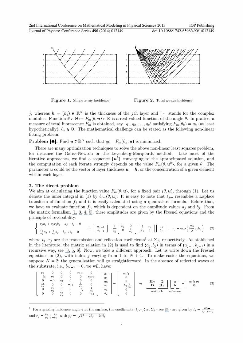
Figure 1. Single x-ray incidence Figure 2. Total x-rays incidence

j, whereas h � phjq P RN is the thickness of the jth layer and | � | stands for the complexmodulus. Function θ P Θ ÞÑ Fmpθ,uq P R is a real-valued function of the angle θ. In pratice, ameasure of total fuorescence Fm is obtained, say tq1, q2, . . . , qvu satisfying Fmpθkq � qk (at leasthypothetically), θk P Θ. The mathematical challenge can be stated as the following non-linearfitting problem:

Problem r♠s: Find u P RN such that qk � Fmpθk,uq is minimized.

There are many optimization techniques to solve the above non-linear least squares problem,for instance the Gauss-Newton or the Levenberg-Marquardt method. Like most of theiterative approaches, we find a sequence tuku converging to the approximated solution, andthe computation of each iterate strongly depends on the value Fmpθ,u

kq, for a given θ. Theparameter u could be the vector of layer thickness u � h, or the concentration of a given elementwithin each layer.

2. The direct problemWe aim at calculating the function value Fmpθ,uq, for a fixed pair pθ,uq, through (1). Let usdenote the inner integral in (1) by `jmpθ,uq. It is easy to note that `jm resembles a Laplacetransform of function fj and it is easily calculated using a quadrature formula. Before that,we have to evaluate function fj , which is dependent on the amplitude values aj and bj . Fromthe matrix formalism [1, 3, 4, 5], these amplitudes are given by the Fresnel equations and theprinciple of reversibility:$&

%νjaj � νjrjbj � aj�1tj � 0

rjνj

aj �1νj

bj � bj�1tj � 0ô

�aj�1

bj�1

��

1

tj

�νj 00 1

νj

� �1 rjrj 1

� �ajbj

�, νj � exp

�i2π

λpjhj

(2)

where tj , rj are the transmission and reflection coefficients1 at Σj , respectively. As stablishedin the literature, the matrix relation in (2) is used to find paj , bjq in terms of paj�1, bj�1q in arecursive way, see [3, 5, 6]. Now, we take a different approach. Let us write down the Fresnelequations in (2), with index j varying from 1 to N � 1. To make easier the equations, wesuppose N � 2; the generalization will go straightforward. In the absence of reflected waves atthe substrate, i.e., bN�1 � 0, we will have:�

�������

ν1 0 0 0 r1ν1 0�t2 ν2 0 0 0 r2ν20 �t3 ν3 0 0 0r1ν1

0 0 �t11ν1

0

0 r2ν2

0 0 �t21ν2

0 0 r3ν3

0 0 �t3

��������

�������

a1a2a3b0b1b2

������� �

��������

a0t100

�b31ν3

00

��������

ô

�HU QD HL

�looooooooomooooooooon

matrix L

�ab

�loomoonunknown

�

�a0t1ρ1

0

�(3)

1 For a grazing incidence angle θ at the surface, the coefficients ptj , rjq at Σj - see [3] - are given by tj �2pj�1

pj�1�pj

and rj �pj�1�pjpj�1�pj

, with pj �aθ2 � 2δj � 2iβj

2nd International Conference on Mathematical Modeling in Physical Sciences 2013 IOP PublishingJournal of Physics: Conference Series 490 (2014) 012149 doi:10.1088/1742-6596/490/1/012149

2

with a � pa1, a2, . . . , aN�1qT and b � pb0, b1, . . . , bN q

T . In the multidimensional case (righthand side of (3)), D � diagrprjν

�1j qs P CpN�1q�pN�1q is a diagonal matrix while HU ,HL P

CpN�1q�pN�1q are the so called Hessenberg matrices, upper and lower respectively. Also,ρj P CN�1 is the jth canonical vector. A similar approach, not exactly in the same matrixcontext, was also stablished in [2]. It should be noted that (3) gives us the following results:

"HUa�Qb � a0t1ρ1

Da�HLb � 0ñ

"a � �D�1HLb�Q�HUD

�1HL

�b � a0t1ρ1

(4)

-3.5-3

-2.5-2

-1.5-1

-0.50

0.51

-2 -1 0 1 2 3 -3.5-3

-2.5-2

-1.5-1

-0.50

0.51

-2 -1 0 1 2 3 -0.5

0

0.5

1

1.5

2

2.5

-2 -1.5 -1 -0.5 0 0.5 1 -0.1

-0.05

0

0.05

0.1

0.15

0.2

-0.2 -0.1 0 0.1 0.2 0.3 0.4

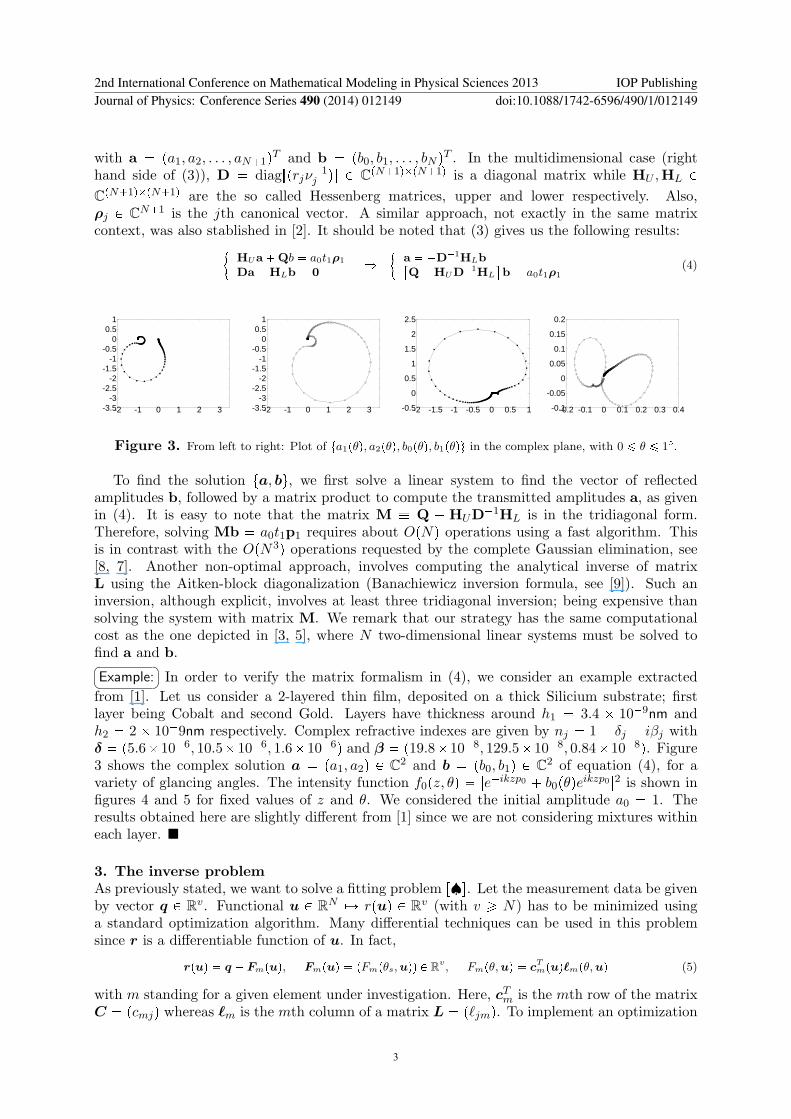
Figure 3. From left to right: Plot of ta1pθq, a2pθq, b0pθq, b1pθqu in the complex plane, with 0 ¤ θ ¤ 1�.

To find the solution ta, bu, we first solve a linear system to find the vector of reflectedamplitudes b, followed by a matrix product to compute the transmitted amplitudes a, as givenin (4). It is easy to note that the matrix M � Q � HUD

�1HL is in the tridiagonal form.Therefore, solving Mb � a0t1p1 requires about OpNq operations using a fast algorithm. Thisis in contrast with the OpN3q operations requested by the complete Gaussian elimination, see[8, 7]. Another non-optimal approach, involves computing the analytical inverse of matrixL using the Aitken-block diagonalization (Banachiewicz inversion formula, see [9]). Such aninversion, although explicit, involves at least three tridiagonal inversion; being expensive thansolving the system with matrix M. We remark that our strategy has the same computationalcost as the one depicted in [3, 5], where N two-dimensional linear systems must be solved tofind a and b.�� ��Example: In order to verify the matrix formalism in (4), we consider an example extracted

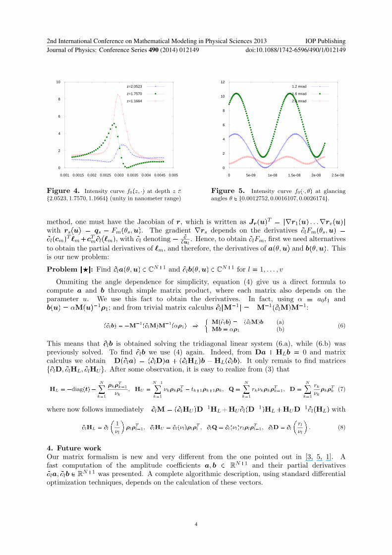
from [1]. Let us consider a 2-layered thin film, deposited on a thick Silicium substrate; firstlayer being Cobalt and second Gold. Layers have thickness around h1 � 3.4 � 10�9nm andh2 � 2 � 10�9nm respectively. Complex refractive indexes are given by nj � 1 � δj � iβj withδ � p5.6�10�6, 10.5�10�6, 1.6�10�6q and β � p19.8�10�8, 129.5�10�8, 0.84�10�8q. Figure3 shows the complex solution a � pa1, a2q P C2 and b � pb0, b1q P C2 of equation (4), for avariety of glancing angles. The intensity function f0pz, θq � |e�ikzp0 � b0pθqe

ikzp0 |2 is shown infigures 4 and 5 for fixed values of z and θ. We considered the initial amplitude a0 � 1. Theresults obtained here are slightly different from [1] since we are not considering mixtures withineach layer. �

3. The inverse problemAs previously stated, we want to solve a fitting problem r♠s. Let the measurement data be givenby vector q P Rv. Functional u P RN ÞÑ rpuq P Rv (with v ¥ N) has to be minimized usinga standard optimization algorithm. Many differential techniques can be used in this problemsince r is a differentiable function of u. In fact,

rpuq � q � Fmpuq, Fmpuq � pFmpθs,uqq P Rv, Fmpθ,uq � cTmpuq`mpθ,uq (5)

with m standing for a given element under investigation. Here, cTm is the mth row of the matrixC � pcmjq whereas `m is the mth column of a matrix L � p`jmq. To implement an optimization

2nd International Conference on Mathematical Modeling in Physical Sciences 2013 IOP PublishingJournal of Physics: Conference Series 490 (2014) 012149 doi:10.1088/1742-6596/490/1/012149

3

0

2

4

6

8

10

0.001 0.0015 0.002 0.0025 0.003 0.0035 0.004 0.0045 0.005

z=2.0523

z=1.7570

z=1.1664

Figure 4. Intensity curve f0pz, �q at depth z Pt2.0523, 1.7570, 1.1664u (unity in nanometer range)

0

2

4

6

8

10

12

0 5e-09 1e-08 1.5e-08 2e-08 2.5e-08

1.2 mrad

1.6 mrad

2.6 mrad

Figure 5. Intensity curve f0p�, θq at glancingangles θ P t0.0012752, 0.0016107, 0.0026174u.

method, one must have the Jacobian of r, which is written as JrpuqT � r∇r1puq . . .∇rvpuqs

with rspuq � qs � Fmpθs,uq. The gradient ∇rs depends on the derivatives BlFmpθs,uq �Blpcmq

T `m�cTmBlp`mq, with Bl denoting �BBul

. Hence, to obtain BlFm, first we need alternatives

to obtain the partial derivatives of `m, and therefore, the derivatives of apθ,uq and bpθ,uq. Thisis our new problem:

Problem r�s: Find Blapθ,uq P CN�1 and Blbpθ,uq P CN�1 for l � 1, . . . , v

Ommiting the angle dependence for simplicity, equation (4) give us a direct formula tocompute a and b through simple matrix product, where each matrix also depends on theparameter u. We use this fact to obtain the derivatives. In fact, using α � a0t1 andbpuq � αMpuq�1ρ1; and from trivial matrix calculus BlrM

�1s � �M�1pBlMqM�1:

pBlbq � �M�1pBlMqM�1pαρ1q ñ

"MpBlbq � �pBlMqb (a)Mb � αρ1 (b)

(6)

This means that Blb is obtained solving the tridiagonal linear system (6.a), while (6.b) waspreviously solved. To find Blb we use (4) again. Indeed, from Da � HLb � 0 and matrixcalculus we obtain �DpBlaq � pBlDqa � pBlHLqb � HLpBlbq. It only remais to find matricestBlD, BlHL, BlHUu. After some observation, it is easy to realize from (3) that

HL � �diagptq �N

k�1

ρkρTk�1

νk, HU �

N�1

k�1

νkρkρTk � tk�1ρk�1ρk, Q �

N

k�1

rkνkρkρTk�1, D �

N

k�1

rkνk

ρkρTk (7)

where now follows immediately �BlM � pBlHU qD�1HL�HUBlpD

�1qHL�HUD�1BlpHLq with

BlHL � Bl

�1

νl

ρlρ

Tl�1, BlHU � Blpνlqρlρ

Tl , BlQ � Blpνlqrlρlρ

Tl�1, BlD � Bl

�rlνl

. (8)

4. Future workOur matrix formalism is new and very different from the one pointed out in [3, 5, 1]. Afast computation of the amplitude coefficients a, b P RN�1 and their partial derivativesBla, Blb P RN�1 was presented. A complete algorithmic description, using standard differentialoptimization techniques, depends on the calculation of these vectors.

2nd International Conference on Mathematical Modeling in Physical Sciences 2013 IOP PublishingJournal of Physics: Conference Series 490 (2014) 012149 doi:10.1088/1742-6596/490/1/012149

4

References[1] de Boer D K G, 1991 Glancing-incidence x-ray fluorescence of layered materials, Physical Review B, 42(2), pp. 498.[2] Perez R D, Sanchez H J, Rubio M, Perez C A, 1999 Mathematical model for evaluation of surface analysis data by

total reflection xrf, X-Ray Spectrometry, 28, pp.342.[3] Sanchez H J, Perez C A, Perez R D, Rubio M, 1996 Surface analysis by total-reflection x-ray fluorescence,

Radiat.Phys.Chem. 48, pp.325.[4] Parrat L G, 1994 Surface studies of solids by total reflection of x-rays, Physical Review, 95(2), pp 359.[5] Krol A, Sher C J and Kao Y H, 1988 X-ray fluorescence of layered synthetic materials with interfacial roughness, Phyical

Review B, 38(13), 8579-92.[6] Gerrard A and Burch J M, 1975, Introduction to Matrix Methods in Optics, Dover, John Wiley & Sons.[7] Lewis J W, 1982 Inversion of tridiagonal matrices, Numerische Mathematik, 38(3), pp.333.[8] Usmani R A, 1994 Inversion of jacobi’s tridiagonal matrix, Computer Math. Applic., 27(8), pp.59.[9] Tian Y, Takane Y, 2009 The inverse of any two-by-two nonsingular partitioned matrix and three matrix inverse

completion problems, Computers & Mathematics with Applications, 57(8), pp. 12941304.

2nd International Conference on Mathematical Modeling in Physical Sciences 2013 IOP PublishingJournal of Physics: Conference Series 490 (2014) 012149 doi:10.1088/1742-6596/490/1/012149

5