Nonlinear control design for wave
energy converter
Galván García, Bruno
First supervisor: Bayu Jayawardhana
Second supervisor: Antonis I. Vakis
Master’s Thesis
Industrial Engineering
August 2014
Abstract
In this thesis, we study the optimization of a single-piston pump system for use in a new wave
energy converter by using a feedback mechanism.
The first part of the thesis is dedicated to the optimal determination of control variables using the
dynamical model of the single-piston pump system, which is a switched system that is built on first
principles and describes the dynamics of four main important elements of the system: the buoy, the
rod, the piston and the pumped water. Using the Analysis of Variance method, it is found that the
two optimum control variables are the area of the piston, as expected, and the mass of the buoy.
The second part of the thesis deals with the design of optimal feedback control where the area of
the piston is the chosen control variable. The control method is based on the well-known Model
Predictive Control that has been adjusted to our switched system. Our simulation results show that
the proposed control method is able to reach performance close to the optimal one.

Acknowledgments
I would like to express my deep gratitude to Prof. Dr. Bayu Jayawardhana and Dr. Antonis I. Vakis,
my research supervisors, for their patient guidance, enthusiastic encouragement and useful critiques
of this research work. I would also like to thank Drs. W.A. Prins and all the members of the Ocean
Grazer Group for their help and assistance in several points of this thesis.
My thanks is also extended to the technicians of the laboratory of the DTPA department for their
support offering me the resources in running different programs.
I owe my heartfelt gratitude towards my mother Emma García for her continuous support and
encouragement throughout my thesis; my grateful thanks are also extended to my father Fernando
Galván, my sister Sandra and my girlfriend Ana.

1
Contents
1 Introduction ......................................................................................................................................... 3
1.1 Renewable Energies. ..................................................................................................................... 3
1.2 Ocean Grazer................................................................................................................................. 4
1.2.1 Introduction ........................................................................................................................... 4
1.2.2 Ocean Grazer Consortium ...................................................................................................... 4
1.2.3 Multi-Piston Multi-Pump Power Take-off System ................................................................. 4
1.3 Why is necessary the control? ...................................................................................................... 5
1.4 Current work in the Ocean Grazer Project.................................................................................... 6
1.5 Contributions of the thesis ........................................................................................................... 7
2 Dynamical Model for the Single Piston Pump...................................................................................... 8
2.1 Previous Model ............................................................................................................................. 8
2.2 New dynamical model ................................................................................................................ 11
2.3 Simulation setup ......................................................................................................................... 13
2.4 Simulation results ....................................................................................................................... 14
3 Control variable determination ......................................................................................................... 18
3.1 First approximation to determine the most influent parameters .............................................. 18
3.2 Analysis of variance ..................................................................................................................... 19
3.3 Choice of the control variable ..................................................................................................... 25
4 Control strategy for the Ocean Grazer ............................................................................................... 26
4.1 Choice of the control strategy .................................................................................................... 26
4.2 Theoretical introduction to MPC ................................................................................................ 27
4.3 Modification of the MPC for the switched systems .................................................................... 30
4.4 Optimization problem ................................................................................................................. 31
4.4.1 Introduction to ICLOCS toolbox ........................................................................................... 31
4.4.2 Choice of the cost function .................................................................................................. 32
4.4.3 Implementation of the SPP model into ICLOCS ................................................................... 34
4.4.4 Toolbox results analysis ....................................................................................................... 36
4.4.5 Exhaustive search ................................................................................................................. 38
4.5 Implementation of the MPC ....................................................................................................... 39

2
4.6 Lookup table as an alternative control strategy ......................................................................... 41
4.7 Results analysis ........................................................................................................................... 43
4.7.1 Comparison of Controller results ......................................................................................... 43
4.7.2 Effects of varying the time-step ........................................................................................... 46
4.7.3 Comparison using or not MPC controller ............................................................................ 47
4.7.4 Comparison with a significant number of input waves. ...................................................... 49
5 Conclusions & Future work ................................................................................................................ 53
Appendix A ............................................................................................................................................ 54
A.1 Dynamical Model ........................................................................................................................ 54
A.2 ICLOCS toolbox setup .................................................................................................................. 58
A.3 Programs developed for the Control .......................................................................................... 65
A.3.1 Lookup table simulations ..................................................................................................... 65
A.3.2 Exhaustive search ................................................................................................................ 67
A.3.3 Implementation of the MPC ................................................................................................ 67
A.4 Different responses changing different parameters .................................................................. 71
Bibliography .......................................................................................................................................... 72
3
Chapter 1
Introduction
1.1 Renewable Energies. Since the Industrial Revolution, fossil fuels have been used as the primary resource for energy.
However, during the last years several problems have been caused by the energy policy of using
non-renewable energies. First of all, fossil fuels need a very long time to be produced by the earth
and their extraction rate is much higher than the production rate. Furthermore, in the last years of
the 20th century there was a change in the energy policy that aims to reduce emissions of CO2
(which, according to [1] is one of the major causes of global warming). Despite the fact that
estimations of how many non-renewable energy sources are left for exploitation will vary due to
technological advances, it is quite clear that fossil fuels will be expensive and rare to find during the
next years.
Renewable energy sources are defined as the energy sources that are derived from natural sources
that replenish themselves over short periods of time [2]. Nowadays, a huge investment in money
and research in the development of renewable energy is being done. In 2009, 18.2% of the total
electricity produced proceeded from renewable resources, while in 2011 this increased to 20.4% and
to 23.4% in 2012 [3].
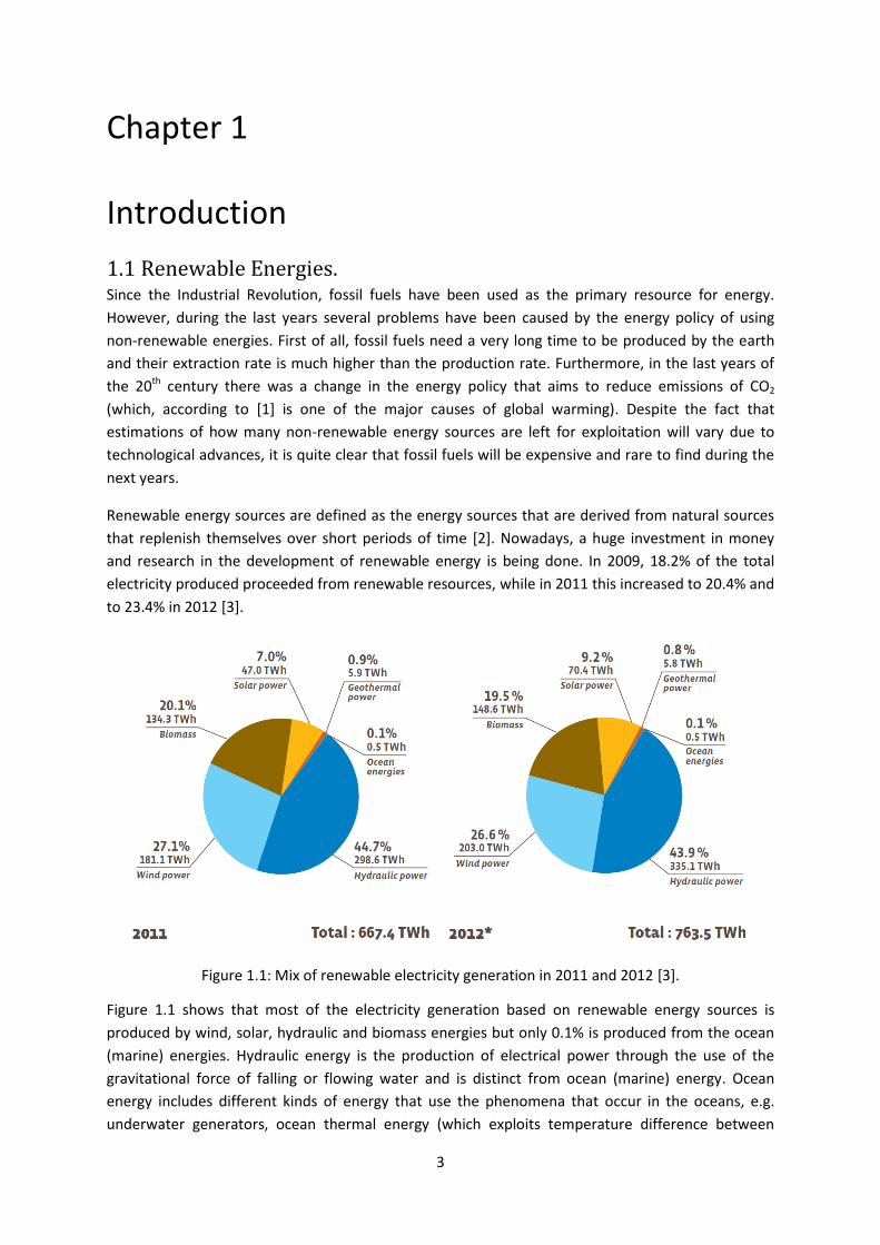
Figure 1.1: Mix of renewable electricity generation in 2011 and 2012 [3].
Figure 1.1 shows that most of the electricity generation based on renewable energy sources is
produced by wind, solar, hydraulic and biomass energies but only 0.1% is produced from the ocean
(marine) energies. Hydraulic energy is the production of electrical power through the use of the
gravitational force of falling or flowing water and is distinct from ocean (marine) energy. Ocean
energy includes different kinds of energy that use the phenomena that occur in the oceans, e.g.
underwater generators, ocean thermal energy (which exploits temperature difference between

4
water at different depths), etc., but wave energy conversion offers the highest theoretical energy
potential [3]. Therefore, it seems reasonable to focus future investigations to finding out how
different ocean energies can be harnessed.
1.2 Ocean Grazer
1.2.1 Introduction This thesis is part of a large project termed the Ocean Grazer. The core technology of the Ocean
Grazer is a novel semi-submersible wave energy converter (WEC) that has been patented by the
University of Groningen. The Ocean Grazer project is an ambitious, innovative and long-term project
that offers students a possibility for research, and also aims to be realized outside the educational
environment.
The Ocean Grazer’s WEC consists of three major subcomponents, which are the structure, the
energy production and the energy storage system. Most investments and investigations in previous
wave energy converters are focused on energy production without considering the storage of
energy. Years of investigation are needed in all the fields; however, this thesis focuses on energy
production.
Despite the current investigations are focused on the wave energy converter part of the Ocean
Grazer, the wave energy is not the only energy source that the Ocean Grazer will use. The natural
energy is converted into electrical energy using power take-off systems (PTO) and 5 PTO’s have been
considered for the Ocean Grazer. The PTO1 denotes the primary power take-off system (also known
as multi-piston multi-pump power take-off system or MP2PTO), which is the core technology of the
Ocean Grazer and will contribute about 80% of power generation (a single Ocean Grazer device is
projected to produce more than 200GWh/year [4]). This is but one of the PTOs considered for the
full-scale system; these are discussed in [5].
1.2.2 Ocean Grazer Consortium The Ocean Grazer Project requires a lot of research and funds for realization. Because of this, at the
end of 2013 a consortium was established with the aim of combining knowledge and facilities for
developing the Ocean Grazer. The consortium is headed by the University of Groningen, and current
research partners are Eurofibers (Netherlands), National Technical University of Athens (Greece),
Instituto Superior Technico (Portugal), Imperial College of London (England), KN Ocean Energy
(Denmark), Aalborg University (Denmark), Hydraulics & Maritime Research Centre (Denmark),
Fraunhofer IWES (Germany).
The search of new partners for joining the Ocean Grazer Consortium is always on. The consortium,
as the Ocean Grazer Project, is in its very first steps and nowadays most part of the research is being
done in the University of Groningen.
1.2.3 Multi-Piston Multi-Pump Power Take-off System The operating principle of the MP2PTO system (Figure 1.2) is to create pressure difference in the
working fluid circulating between two reservoirs. This pressure difference (or hydraulic head, ) can
be transformed into electricity via a turbine (T) when the working fluid in the upper reservoir returns
to the lower reservoir. The MP2PTO has some similarities with previously developed point-absorber
systems. However, the main difference among them is the adaptability of the MP2PTO. As shown in

5
Figure 1.2, the MP2PTO consists of multiple interconnected buoys (termed as a floater blanket) and
each buoy is connected to a hydraulic multi-piston pump; the first pump unit can potentially extract
more energy than the second, and so on. Sea waves have an inherent variability in height and
period, and to account for this variability in the energy content of the waves multiple pistons can be
activated within each pump in the MP2PTO system to maximize energy extraction for waves ranging
in height from 1 to 12 meters and periods of 4 to 20 seconds [6] [7].
Figure 1.2: The MP2PTO system.
Preliminary work has demonstrated the successful potential use of a variable-load control for a
multi-piston pump [8].
1.3 Why is control necessary? It is important to realize that the waves that can affect the WEC can vary in height and period [6] [7].
In order to maximize the amount of energy extracted the coupling between any buoy and a number
of variable-size pistons should be controlled because it can optimize the load the buoy has to carry
during the upstroke movement. A wave of great height will contain a lot of energy and vice versa.
Optimum energy extraction can be achieved by tuning the amount of working fluid pumped by each
wave, and hence the load that the wave must support, to its energy content: large loads (multiple
pistons engaged simultaneously) for large waves and small loads (fewer pistons) for small waves.
Equivalently, a multi-piston pump system where multiple pistons can be engaged to alter the
amount of working fluid pumped with each stroke (and hence the load), can be represented using a
single-piston pump (SPP) model where the cross-sectional area of the piston, and hence the
pumping volume, is considered to be a variable. The aim of this thesis is to design a control strategy
to maximize the efficiency of the WEC based on a SPP model with variable piston cross-sectional
area.
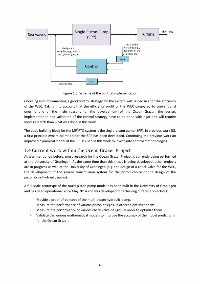
In the Figure 1.3 is shown a scheme of how the control will work on the SPP.
6
Figure 1.3: Scheme of the control implementation
Choosing and implementing a good control strategy for the system will be decisive for the efficiency
of the WEC. Taking into account that the efficiency profit of this WEC compared to conventional
ones is one of the main reasons for the development of the Ocean Grazer, the design,
implementation and validation of the control strategy have to be done with rigor and will require
more research than what was done in this work.
The basic building block for the MP2PTO system is the single-piston pump (SPP). In previous work [8],
a first principle dynamical model for the SPP has been developed. Continuing the previous work an
improved dynamical model of the SPP is used in this work to investigate control methodologies.
1.4 Current work within the Ocean Grazer Project As was mentioned before, most research for the Ocean Grazer Project is currently being performed
at the University of Groningen. At the same time than this thesis is being developed, other projects
are in progress as well at the University of Groningen (e.g. the design of a check valve for the WEC,
the development of the geared transmission system for the piston choice or the design of the
piston-type hydraulic pump).
A full-scale prototype of the multi-piston pump model has been built in the University of Groningen
and has been operational since May 2014 and was developed for achieving different objectives:
- Provide a proof-of-concept of the multi-piston hydraulic pump.
- Measure the performance of various piston designs, in order to optimize them.
- Measure the performance of various check valve designs, in order to optimize them.
- Validate the various mathematical models to improve the accuracy of the model predictions
for the Ocean Grazer.
7
1.5 Contributions of the thesis As was explained before, the development of the Ocean Grazer is in its very first steps, and only the
potential use of control for the Ocean Grazer has been demonstrated in [8].
The main contributions of this thesis are:
1- Improvement of the previous first principle dynamical model [8]. The better the dynamical
model is, the more accurate the results. (Chapter 2)
2- Optimal determination of the control variables. The Analysis of Variance (ANOVA) method
and the SPP model have been used for this purpose. (Chapter 3)
3- Design and implementation of the optimal feedback control where the area of the piston is
the chosen control variable. The control method is based on Model Predictive Control
(MPC). (Chapter 4).
With these contributions we aim to improve the dynamical model and make the first steps in the
control field. Furthermore, the advantage of using a control strategy is checked conclusively (section
4.7.3).

8
Chapter 2
Dynamical Model for the Single Piston
Pump
2.1 Previous Model As was mentioned before, the starting point of this work is a previous thesis [8], where a dynamical
model was developed for the wave energy converter.
The nomenclature and parameters that are used in this thesis are summarized in Table 2.1.
Variable Symbol Value Units
Gravity constant g 9.81 m/s2
Free water density ρ 1000 kg/m3
Sea water density ρsw 1030 kg/m3
Free water viscosity μ 1.002 Pa·s
Steel density ρsteel 7850 kg/m3
Steel young’s modulus Esteel 210·109 Pa
Rod damping ratio 0.01 -
Rod radius Rrod 0.04 m
Rod length Lr 140 m
Mass of the buoy m1 1000 kg
Mass of the piston mp 500 kg
Mass of the rod mr 5.52·103 kg
Surface of the buoy Sb 49 m2
Height of the buoy Hb 2 m
Height of the piston Hpist 0.1 m
Radius of the piston Rp 0.2 m
Separation piston-cylinder spist 10-3 m
Length of the cylinder Lc 100 m
Volume of the Up. Res. VU 1000 m3
Area of the Up. Res. AU 49 m2
Volume of the Low. Res. VL 1000 m3
Area of the Low. Res. AL 49 m2
Table 2.1: Data table of used values.
The SPP was modelled with dynamical elements in [8] as follows
9
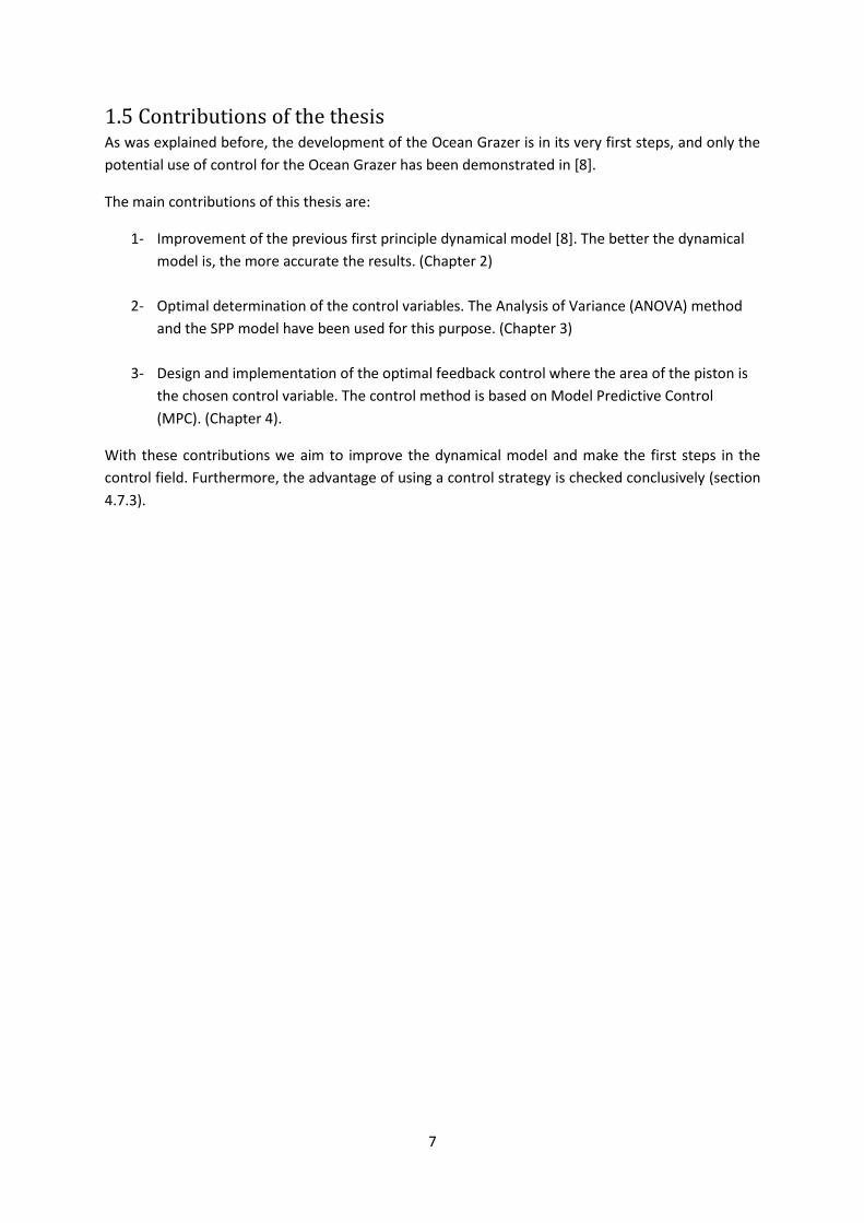
Figure 2.1: Single-piston pump modelled with dynamical elements [8].
The buoy is modelled as a rectangular prism with mass . This is connected by a rod to the piston,
modelled as a mass that also considers the mass corresponding to the rod. The rod will be
tensioned during the upstroke movement with the tension decreasing during the downstroke. In
order to model this part, a rigid steel rod is considered, modelled as an ideal spring with stiffness
. The friction between the piston and the cylinder was modelled with a damper with
a damping coefficient
corresponding to the formulation of viscous friction
(Couette flow). For more insightful physical interpretations of the dynamical model, we refer the
interested reader to [8].
The dynamical model in [8] is described by a space-state equation
( ) (2.1)
where the state vector is given by
[ ] , (2.2)
with being the position of the buoy’s centre of mass (in m), being the velocity of the buoy (in
m/s), being the position of the piston’s centre of mass (in m), being the velocity of the piston
(in m/s) and and being the pressures of the upper and lower reservoir respectively (in Pa).
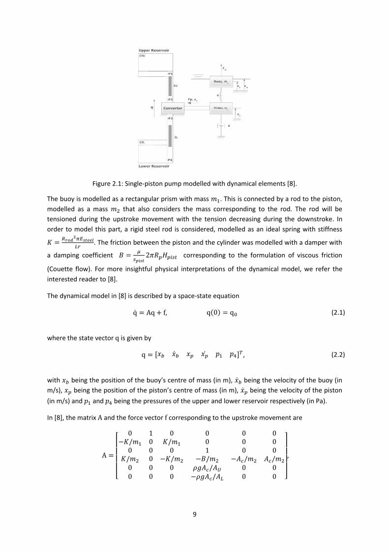
In [8], the matrix and the force vector corresponding to the upstroke movement are
[
]
,
10
and
[
( )
]
(2.3)
where Fb is the buoyancy force (which depends on the position of the buoy and the position of
the wave ), i.e. the force that the incident wave exerts on the buoy, and is formulated by
( ) {
(
)
(2.4)
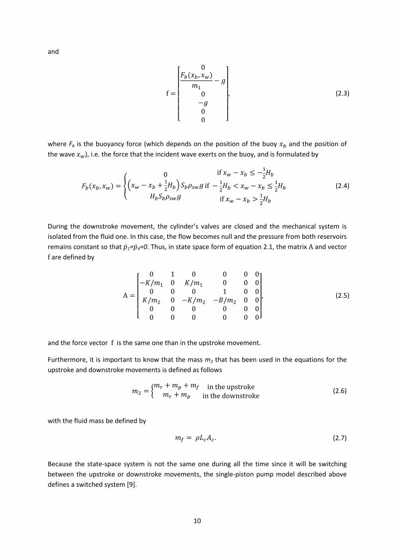
During the downstroke movement, the cylinder’s valves are closed and the mechanical system is
isolated from the fluid one. In this case, the flow becomes null and the pressure from both reservoirs
remains constant so that 1= 4=0. Thus, in state space form of equation 2.1, the matrix and vector
are defined by
[
]
, (2.5)
and the force vector is the same one than in the upstroke movement.
Furthermore, it is important to know that the mass m2 that has been used in the equations for the
upstroke and downstroke movements is defined as follows
{
(2.6)
with the fluid mass be defined by
. (2.7)
Because the state-space system is not the same one during all the time since it will be switching
between the upstroke or downstroke movements, the single-piston pump model described above
defines a switched system [9].

11
2.2 New dynamical model In the dynamical model developed in [8], there are different forces that were not considered. In the
absence of damping (caused by many friction forces), as it can be observed when solving the
differential equation for the buoy ( ) , the hydrostatic stiffness will result in
higher-frequency buoy vibrations.
In the single piston pump there exists a friction force at the piston-cylinder interface that has been
considered in [8], where a linear damper (with damping coefficient ) between the cylinder wall
(considered as a fixed part) and the piston has been used for this purpose. Furthermore, the rod is
considered as a steel rod of length and there are energy losses between the rod and the
water, between the fibers of the rod itself (internal friction) as well as frictional contact at secondary
interfaces, which result in losses of energy to the system [7] and cannot be neglected. These friction
forces haven’t been considered in [8] and their inclusion in the modeling is expected to reduce the
amount of vibrations which were obtained previously in [8].
In order to include some of the energy losses explained above in the dynamical model we consider a
linear damper that is connected to the buoy and the piston. Such a damper is a first approximation
to the damping in the rod itself. The damping ratio ζ is related to the damping coefficient via the
expression √ .
The new dynamical model of the single piston pump model is illustrated in the Figure 2.2.
Figure 2.2: Dynamical model of the single-piston pump.
In this new dynamical model, the reference point for all the displacements has been changed
compared to [8]. In our modelling, the reference point for and is the centre of mass (COM) of
the piston. Hence, in comparison to [8], we have the following relations
(2.8)
(2.9)

12
where and are the displacement of the buoy and the wave in [8] respectively, and
and are the displacement of the buoy and the wave in the new model. Because of
this, there will be a new term (which doesn’t appear in the equations of the previous model) that
will appear on the equations of motion for the buoy and the piston.
The damper with coefficient explained above will appear in the equations of motion for the buoy
and the piston as follows
Buoy: ( )⏟
( ) (2.10)
Piston: ( )⏟
( ) ( ) (2.11)
where is an initial approximation of the friction between the piston and the cylinder
wall.
Moreover, the amount of water that the piston has to pump in every upstroke is not only the water
in the cylinder but also the water inside the upper reservoir, as shown in the Figure 2.2. Because of
this, the fluid mass (appeared in the mass ) has to be modified as follows
( * (2.12)
(c.f. the formulation of in the equation 2.7 as used in [8]).
With all these considerations we can modify the previous switched system where in the upstroke
movement we use
[
]
,
[
]
(2.13)
while in the downstroke movement we use
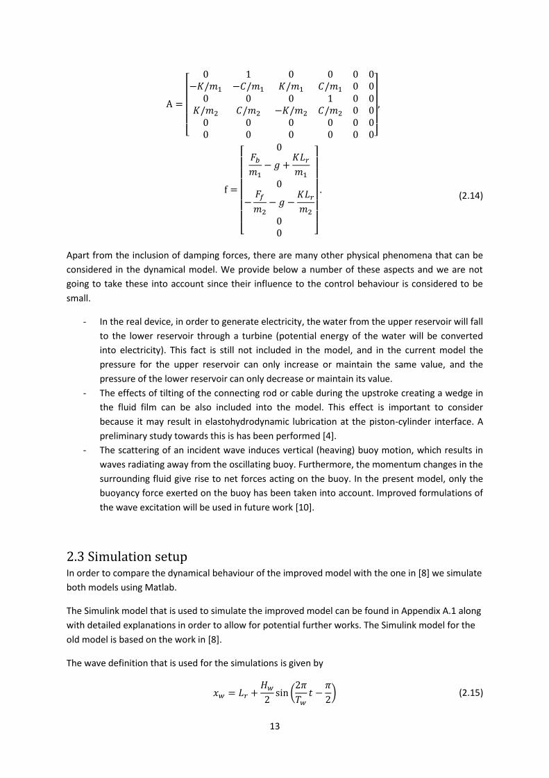
13
[
]
[
]
(2.14)
Apart from the inclusion of damping forces, there are many other physical phenomena that can be
considered in the dynamical model. We provide below a number of these aspects and we are not
going to take these into account since their influence to the control behaviour is considered to be
small.
- In the real device, in order to generate electricity, the water from the upper reservoir will fall
to the lower reservoir through a turbine (potential energy of the water will be converted
into electricity). This fact is still not included in the model, and in the current model the
pressure for the upper reservoir can only increase or maintain the same value, and the
pressure of the lower reservoir can only decrease or maintain its value.
- The effects of tilting of the connecting rod or cable during the upstroke creating a wedge in
the fluid film can be also included into the model. This effect is important to consider
because it may result in elastohydrodynamic lubrication at the piston-cylinder interface. A
preliminary study towards this is has been performed [4].
- The scattering of an incident wave induces vertical (heaving) buoy motion, which results in
waves radiating away from the oscillating buoy. Furthermore, the momentum changes in the
surrounding fluid give rise to net forces acting on the buoy. In the present model, only the
buoyancy force exerted on the buoy has been taken into account. Improved formulations of
the wave excitation will be used in future work [10].
2.3 Simulation setup In order to compare the dynamical behaviour of the improved model with the one in [8] we simulate
both models using Matlab.
The Simulink model that is used to simulate the improved model can be found in Appendix A.1 along
with detailed explanations in order to allow for potential further works. The Simulink model for the
old model is based on the work in [8].
The wave definition that is used for the simulations is given by
(
* (2.15)
14
The initial condition of the state variables used in all simulations are given by
[
]
(2.16)
This initial condition represents the rest conditions of the system in calm water (i.e., no wave).
and are the initial heights of working fluid in the upper and lower reservoir respectively so the
initial conditions of the pressures and are the corresponding hydrostatic pressures.
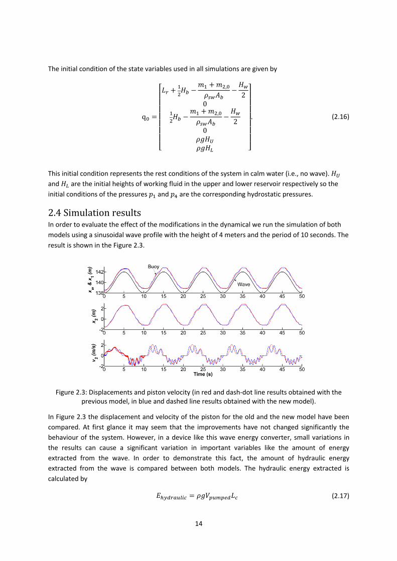
2.4 Simulation results In order to evaluate the effect of the modifications in the dynamical we run the simulation of both
models using a sinusoidal wave profile with the height of 4 meters and the period of 10 seconds. The
result is shown in the Figure 2.3.
Figure 2.3: Displacements and piston velocity (in red and dash-dot line results obtained with the previous model, in blue and dashed line results obtained with the new model).
In Figure 2.3 the displacement and velocity of the piston for the old and the new model have been
compared. At first glance it may seem that the improvements have not changed significantly the
behaviour of the system. However, in a device like this wave energy converter, small variations in
the results can cause a significant variation in important variables like the amount of energy
extracted from the wave. In order to demonstrate this fact, the amount of hydraulic energy
extracted from the wave is compared between both models. The hydraulic energy extracted is
calculated by
(2.17)
15
where is the density of the water, the length of the cylinder and the volume of water
pumped. Under the same conditions (e.g. the wave and initial conditions), the energy obtained using
the old model is and using the new model is
.
Hence, we obtain an energy difference of , which is a quite significant amount of energy for
the 50 seconds of the simulation.
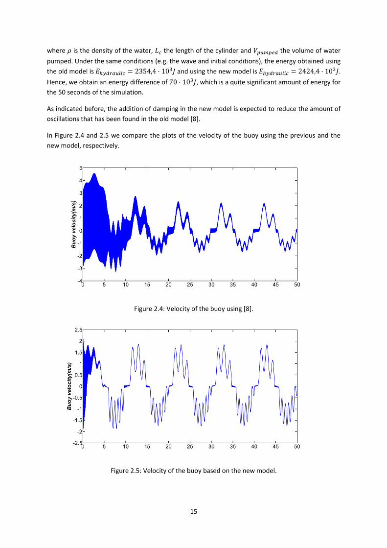
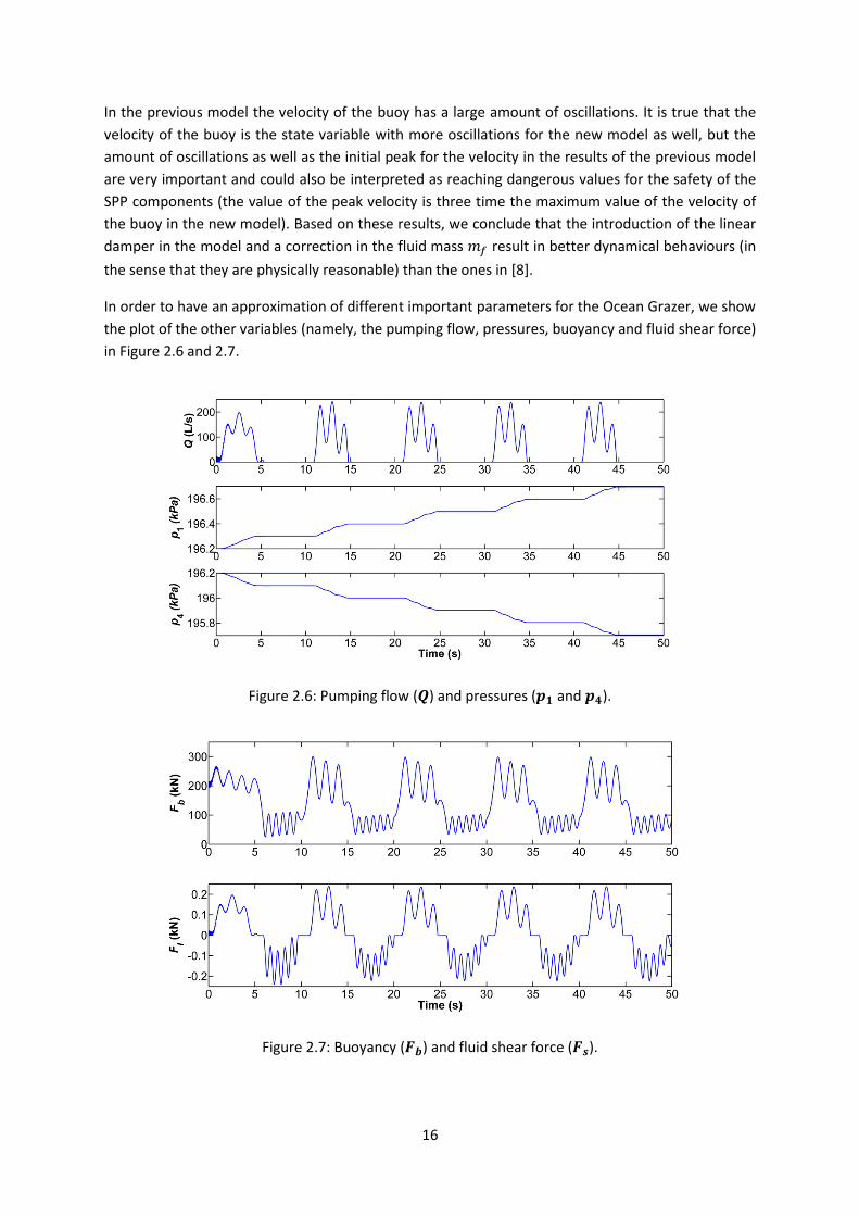
As indicated before, the addition of damping in the new model is expected to reduce the amount of
oscillations that has been found in the old model [8].
In Figure 2.4 and 2.5 we compare the plots of the velocity of the buoy using the previous and the
new model, respectively.
Figure 2.4: Velocity of the buoy using [8].
Figure 2.5: Velocity of the buoy based on the new model.
16
In the previous model the velocity of the buoy has a large amount of oscillations. It is true that the
velocity of the buoy is the state variable with more oscillations for the new model as well, but the
amount of oscillations as well as the initial peak for the velocity in the results of the previous model
are very important and could also be interpreted as reaching dangerous values for the safety of the
SPP components (the value of the peak velocity is three time the maximum value of the velocity of
the buoy in the new model). Based on these results, we conclude that the introduction of the linear
damper in the model and a correction in the fluid mass result in better dynamical behaviours (in
the sense that they are physically reasonable) than the ones in [8].
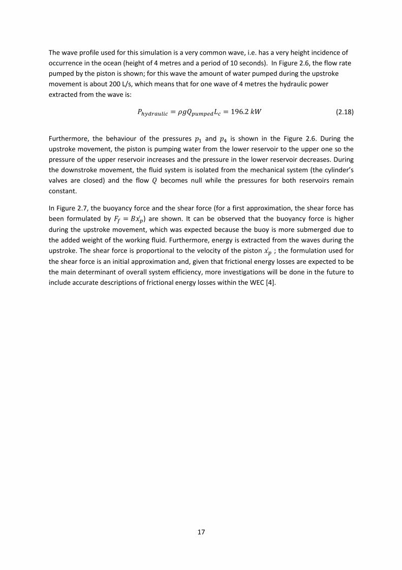
In order to have an approximation of different important parameters for the Ocean Grazer, we show
the plot of the other variables (namely, the pumping flow, pressures, buoyancy and fluid shear force)
in Figure 2.6 and 2.7.
Figure 2.6: Pumping flow ( ) and pressures ( and ).
Figure 2.7: Buoyancy ( ) and fluid shear force ( ).
17
The wave profile used for this simulation is a very common wave, i.e. has a very height incidence of
occurrence in the ocean (height of 4 metres and a period of 10 seconds). In Figure 2.6, the flow rate
pumped by the piston is shown; for this wave the amount of water pumped during the upstroke
movement is about 200 L/s, which means that for one wave of 4 metres the hydraulic power
extracted from the wave is:
(2.18)
Furthermore, the behaviour of the pressures and is shown in the Figure 2.6. During the
upstroke movement, the piston is pumping water from the lower reservoir to the upper one so the
pressure of the upper reservoir increases and the pressure in the lower reservoir decreases. During
the downstroke movement, the fluid system is isolated from the mechanical system (the cylinder’s
valves are closed) and the flow becomes null while the pressures for both reservoirs remain
constant.
In Figure 2.7, the buoyancy force and the shear force (for a first approximation, the shear force has
been formulated by ) are shown. It can be observed that the buoyancy force is higher
during the upstroke movement, which was expected because the buoy is more submerged due to
the added weight of the working fluid. Furthermore, energy is extracted from the waves during the
upstroke. The shear force is proportional to the velocity of the piston ; the formulation used for
the shear force is an initial approximation and, given that frictional energy losses are expected to be
the main determinant of overall system efficiency, more investigations will be done in the future to
include accurate descriptions of frictional energy losses within the WEC [4].
18
Chapter 3
Control variable determination
3.1 First approximation to determine the most influent parameters As a first step toward the design of optimal feedback control for the single piston pump, we need to
determine the optimal control variable. In [8], it has been assumed that the area of the piston is the
optimal control variable. As stated previously, one of the main innovations of the Ocean Grazer WEC
is the adaptability of energy extraction to the energy content of individual waves through the
variation of pumped volume (and load) per wave period, which can be achieved by varying the net
effective cross-sectional area of the piston(s).
The control variables that will be chosen will be ones that can be physically manipulated and have an
important influence on the behaviour of the system. In this regard, we consider the following five
variables that will be used to define the important behaviours of the system:
- Volume pumped per wave period, denoted by and calculated by
( ) ( )
(3.1)
where is the time when the piston is at the bottom of the cylinder and is the period of
the wave.
- Maximum of piston’s velocity, denoted by .
- Maximum distance between the wave and the buoy, denoted by ‖ ‖ and defined
by
‖ ‖ [ ]
| ( ) ( )|
where is the terminal time.
- L2 distance between the wave and the buoy ‖ ‖ , measured in the following way
‖ ‖ (∫ | ( ) ( )|
)
(3.2)
where is the final time of the simulation.
- Worst case of rod’s tension denoted by and calculated by

19
( (
[ ]
( )
))
[ ] ( ) (3.3)
where is the buoyancy force, the area of the cylinder and is the length of the
cylinder.
Based on the dynamical behaviour of these five variables, we can calculate the total energy gained,
determine the fluctuation variation of the buoy profile with respect to the wave profile and the
minimum requirements for the rod in terms of the material yield and ultimate strengths.
In order to have a first approximation about which could be the optimal control variables, the five
variables explained above are calculated for varying different parameters of the system (e.g. the
mass of the buoy, the mass of the rod, the piston area etc.). It is important to realize that only one
parameter is modified at each time.
The different parameters that are modified, the values that are used, and the values of the five
different variables are shown in the Appendix A.4. In this table it can be seen that the values of the
volume pumped and the distance between the wave and the buoy change considerably when we
modify the value of the area of the piston. The volume pumped and the distance between the buoy
and the wave increases with increasing the area of the piston. Furthermore, the mass of the buoy
seems to also be important for the distance between the wave and the buoy: increasing the mass of
the buoy reduces that distance. The other parameters do not seem to have a very important role in
the behaviour of the system. Therefore, we conclude that the area of the piston and the mass of the
buoy (to a lesser extent) seem to be the best candidates for being the control variables.
Since the area of the piston is one of the potential candidates for being the control variable several
simulations are run varying its value. When the value of the piston’s area increases the
area of the cylinder ( ) increases as well because the separation between the piston
and the cylinder wall is a constant value.
3.2 Analysis of Variance In order to confirm if the area of the piston’s cylinder and the mass of the buoy have a significant
influence on the behaviour of the system, we perform a factorial analysis of variance [11].
This analysis of variance (ANOVA) study uses a block design and considers two factors (the area of
the cylinder and the mass of the buoy):
- We want to know if the response (variable Y ) has the same values in the different levels of
the factor 1. These values can depend on another factor 2.
- The factor 1 (area of the cylinder) has 4 levels ( ) and the factor 2 (mass of the buoy), 3
levels ( ).
- For each level of the area of the cylinder there are 3 values of Y (one for each level of the
buoy’s mass). In total, there are values of the response Y.
- The response (variable Y ) will be the volume pumped per stroke and the distance between
the wave and the buoy (one ANOVA per each response).

20
First of all, let us define the response for each level i of the factor 1 and for each level j of the factor
2
(3.4)
where is the average of Y , is the effect of the level i of the factor 1 in the global average , is
the effect of the level j of the factor 2 in the global average and is the random variability of .
In the analysis of variance method, we calculate the sum of squares for each factor and the residual
sum of squares in order to accept or decline the null hypothesis (the considered factor has not a
significant influence in the global average ) and accept or decline the alternative hypothesis (the
considered factor has a significant influence in the global average ).
The hypotheses are the following:
Factor 1 (area of the cylinder)
(3.5)
Factor 2 (mass of the buoy)
(3.6)
The unknown parameters are the following: , where is the variance of
the response . In order know the value of these parameters and conclude if we can accept or
decline the null or the alternative hypothesis, the developed model (section 2.2) is used.
Based on the average of each level of the factor 1 , the average of each level of the factor 2
and average of all the measurements , we get the estimations of the parameters ( ) with
the following formulas [12]:
∑∑
(3.7)
∑( )
(3.8)
∑( )
(3.9)
( )( )∑∑( )
(3.10)

21
Mass of the buoy (kg)
500 1000 2000 0.12 0.4913 0.4917 0.4909 0.4913 -0.3781
0.21 0.7411 0.7445 0.7495 0.7450 -0.1244
0.27 0.9818 0.9886 0.9950 0.9885 0.1190
0.35 1.2493 1.2564 1.2534 1.2530 0.3836
0.8659 0.8703 0.8722 -0.003585 0.00084 0.00274
Table 3.1: Calculation of the estimated parameters (response: Volume pumped per stroke (m2)).
Mass of the buoy (kg)
500 1000 2000 0.12 0.9531 0.9485 0.9349 0.9455 -0.0163
0.21 0.9617 0.9555 0.9438 0.9537 -0.0081
0.27 0.9769 0.9728 0.9619 0.9705 0.0087
0.35 0.9880 0.9814 0.9631 0.9755 0.0157
0.9699 0.9645 0.9509 0.0081 0.0027 -0.0108
Table 3.2: Calculation of the estimated parameters (response: Distance between the wave and the buoy (m)).
For the ANOVA study, the sums of squares (SS ) must be calculated. Using the tables above, the
sums of squares can be calculated by [12] as
∑ ( ) ∑
(3.11)
∑ ( ) ∑
(3.12)
∑ ∑ ( )
(3.13)
∑ ∑ ( )
(3.14)
The sums of squares correspond to the following formula:
(3.15)
Calculating the sums of squares, the following ANOVA tables (one table per each response) are
obtained:
Are
a o
f
the
cylin
der
(m2 )
Are
a o
f
the
cylin
der
(m2 )
22
Sum of squares D.O.F. Variance F statistic Critical F
Factor 1 SSA = 0.959334 3 0.319778 29830.04 4.76
Factor 2 SSB = 8.42617·10-5 2 4.213085·10-5 3.93 5.14
Residual SSR = 6.43205·10-5 6 1.072·10-5
Total SST = 0.9594828 11
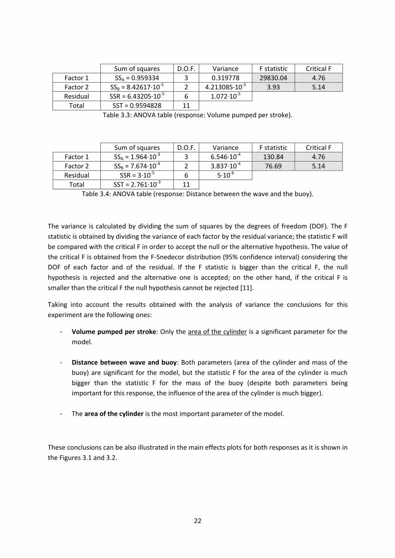
Table 3.3: ANOVA table (response: Volume pumped per stroke).
Sum of squares D.O.F. Variance F statistic Critical F
Factor 1 SSA = 1.964·10-3 3 6.546·10-4 130.84 4.76
Factor 2 SSB = 7.674·10-4 2 3.837·10-4 76.69 5.14
Residual SSR = 3·10-5 6 5·10-6
Total SST = 2.761·10-3 11
Table 3.4: ANOVA table (response: Distance between the wave and the buoy).
The variance is calculated by dividing the sum of squares by the degrees of freedom (DOF). The F
statistic is obtained by dividing the variance of each factor by the residual variance; the statistic F will
be compared with the critical F in order to accept the null or the alternative hypothesis. The value of
the critical F is obtained from the F-Snedecor distribution (95% confidence interval) considering the
DOF of each factor and of the residual. If the F statistic is bigger than the critical F, the null
hypothesis is rejected and the alternative one is accepted; on the other hand, if the critical F is
smaller than the critical F the null hypothesis cannot be rejected [11].
Taking into account the results obtained with the analysis of variance the conclusions for this
experiment are the following ones:
- Volume pumped per stroke: Only the area of the cylinder is a significant parameter for the
model.
- Distance between wave and buoy: Both parameters (area of the cylinder and mass of the
buoy) are significant for the model, but the statistic F for the area of the cylinder is much
bigger than the statistic F for the mass of the buoy (despite both parameters being
important for this response, the influence of the area of the cylinder is much bigger).
- The area of the cylinder is the most important parameter of the model.
These conclusions can be also illustrated in the main effects plots for both responses as it is shown in
the Figures 3.1 and 3.2.

23
0,350,270,210,12
1,3
1,2
1,1
1,0
0,9
0,8
0,7
0,6
0,5
0,4
20001000500
Cylinder Area
Me
an
Mass of the buoy
Main Effects Plot for VpumpedData Means
Figure 3.1: Main effects plot for the
0,350,270,210,12
0,980
0,975
0,970
0,965
0,960
0,955
0,950
0,945
20001000500
Cylinder Area
Me
an
Mass of the buoy
Main Effects Plot for Max distance between buoy waveData Means
Figure 3.2: Main effects plot for the ‖ ‖ .
It is also important to know if interaction exists between the two considered factors (the area of the
piston’s cylinder and the mass of the buoy) [11].

24
20001000500
1,3
1,2
1,1
1,0
0,9
0,8
0,7
0,6
0,5
0,4
Mass of the buoy
Me
an
0,12
0,21
0,27
0,35
Area
Cylinder
Interaction Plot for VpumpedData Means
Figure 3.3: Interaction plot for the
20001000500
0,99
0,98
0,97
0,96
0,95
0,94
0,93
Mass of the buoy
Me
an
0,12
0,21
0,27
0,35
Area
Cylinder
Interaction Plot for Max distance between buoy waveData Means
Figure 3.4: Interaction plot for the ‖ ‖ .
In the Figures 3.3 and 3.4 it can be seen that all the lines are parallel. This means that the effect of
one of the considered factors does not depend on the value of the other factor, so there is no
interaction between the piston’s cylinder area and the mass of the buoy. Therefore, ANOVA results
are validated since there is no interaction between the two considered factors.
25
3.3 Choice of the control variable The goal of the control strategy will be to optimize some function in order to obtain as much energy
as possible, guaranteeing that the buoy follows the wave profile of the system or other
considerations. Because of this, the control variable should be one of the most influent parameters
of the model and, obviously, the control variable must be able to be physically manipulated.
The first option considered for the control variable was the area of the cylinder; after the analysis of
variance it has been confirmed that its value has a significant influence in the volume pumped per
stroke and in the distance between the wave and the buoy. If it is possible to change the area of the
piston’s cylinder during operation of the system then it can be chosen as the control variable.
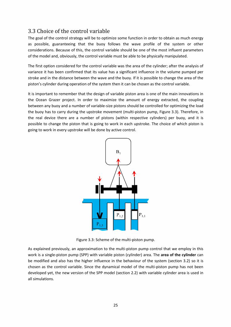
It is important to remember that the design of variable piston area is one of the main innovations in
the Ocean Grazer project. In order to maximize the amount of energy extracted, the coupling
between any buoy and a number of variable-size pistons should be controlled for optimizing the load
the buoy has to carry during the upstroke movement (multi-piston pump, Figure 3.3). Therefore, in
the real device there are a number of pistons (within respective cylinders) per buoy, and it is
possible to change the piston that is going to work in each upstroke. The choice of which piston is
going to work in every upstroke will be done by active control.
Figure 3.3: Scheme of the multi-piston pump.
As explained previously, an approximation to the multi-piston pump control that we employ in this
work is a single-piston pump (SPP) with variable piston (cylinder) area. The area of the cylinder can
be modified and also has the higher influence in the behaviour of the system (section 3.2) so it is
chosen as the control variable. Since the dynamical model of the multi-piston pump has not been
developed yet, the new version of the SPP model (section 2.2) with variable cylinder area is used in
all simulations.

26
Chapter 4
Control strategy for the Ocean Grazer
4.1 Choice of the control strategy The second step in the control design is to choose the most suitable control strategy. This choice will
be made by taking into account the model we have, the goal that is required for the control and the
complexity of the system.
It is known that there are many different control strategies to consider but in this work the
requirement is that the control optimizes, at least, the amount of energy extracted. Moreover, the
dynamical model is a non-linear switched system so simple control strategies, like generic PID
controllers, have been discarded because it won’t be possible to achieve our goals (optimization)
with this kind of controllers [13].
In order to achieve the desired behaviour of the complete SPP system, the control has to meet the
following requirements. Firstly, the optimization problem should be related to the maximization of
the amount of energy extracted from the wave, which is proportional to the (as defined in
equation 3.1), while at the same time aiming to minimize the distance between the buoy and the
wave (i.e., ‖ ‖ or ‖ ‖ ). In addition to this optimization problem, there are state
constraints that have to be taken into account by the controller. These state constraints can have
direct physical interpretations, such as, the upper and lower bound on the displacement of the
piston due to the geometric constraint of the cylinder. Hence, the optimal control has to ensure that
the constraints are not violated so that the safety of the system can be guaranteed.
In this thesis we consider two potential control strategies. One potential control strategy that meets
all of our requirements is the Model Predictive Control (MPC). We will review the basic concept of
MPC in the next section. The MPC method has been used extensively in industry [14]. Some of the
main advantages of using MPC as a control strategy for the Ocean Grazer are:
It can be extended easily to non-linear switched systems;
It takes into account input and output constraints;
It obtains an optimal control input based on known model;
As a kind of feedback control, it has an inherent robustness against disturbances and
uncertainties.
Another potential control strategy is the well-known lookup table, which is a simple control strategy
that has also been used widely in automotive industry, mainly, due to its very low computational
requirements. The comparison between both control strategies will be done in the section 4.7.1.

27
4.2 Theoretical introduction to MPC In the following lines a brief introduction for the Model Predictive Control will be given. For this
explanation, a standard linear discrete time state space system will be considered first as follows
( ) ( ) ( )
(4.1)
( ) ( )
where ( ) and ( ) are model state and input vectors at the time instance.
Model Predictive Control is formulated as a recursive computation of a finite horizon open-loop
optimal control problem subject to system dynamics and input and state constraints [15]. Before
going further in the explanations about how the MPC works, we will briefly describe the important
parts of the MPC:
Prediction model: A model which describes the process dynamics is an important element in the
MPC algorithm to predict the state values over the prediction horizon . The prediction of ( ),
i.e. the state values at time , based on the knowledge available at time will be denoted by
( | ). Using (4.1) as the prediction model, it is immediate to check that
( | ) ( ) ∑ ( )
(4.2)
Constraints: The possibility of including constraints in the state space variables is one of the main
motivations behind MPC [15]. In this thesis, we will only consider constraints defined as box
constraints, e.g.
( ) , , (4.3)
( ) , ,
where and are the lower and upper bounds for the input, respectively and and are the
lower and upper bounds for the state values, respectively.
Cost function: The cost function is a positive definite function of the state and input signal that
represents the variable to be optimized by an appropriate design of control input. One of the typical
forms of the cost function is the quadratic form given by:
∑ ( | ) ( | ) ∑ ( ) ( )
(4.4)
where and are the prediction and the control horizon respectively and and are the strictly
positive definite symmetric weighting matrices.
Using the prediction model, constraint formulations and cost function, we can summarize the MPC
algorithm as follows
28
1- Set the initial time step .
2- Compute the optimal input [ ( ) ( ) ( )] that solves the following
optimization problem:
[ ( ) ( )]]
(4.5)
subject to:
( | ) ( ) ∑ ( )
(4.6)
( ) , ,
( ) , .
3- Set the control input at time , by ( ) ( ).
4- Increment and repeat the whole procedure from step 2.
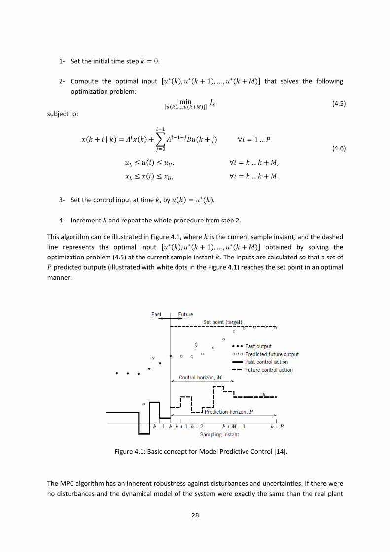
This algorithm can be illustrated in Figure 4.1, where is the current sample instant, and the dashed
line represents the optimal input [ ( ) ( ) ( )] obtained by solving the
optimization problem (4.5) at the current sample instant . The inputs are calculated so that a set of
predicted outputs (illustrated with white dots in the Figure 4.1) reaches the set point in an optimal
manner.
Figure 4.1: Basic concept for Model Predictive Control [14].
The MPC algorithm has an inherent robustness against disturbances and uncertainties. If there were
no disturbances and the dynamical model of the system were exactly the same than the real plant

29
(since we are using the developed SPP model for the simulations, in this case the real plant would be
the full scale SPP prototype) and, furthermore, if the optimization problem could be solved over an
infinite horizon, then the input signal found at could be applied as an open-loop to the system
for all . Nevertheless, the explained situation (no disturbances and perfect match between the
model and the plant) will never happen so it is necessary to incorporate feedback. The recursive
computation of the MPC where every new measurement ( ) is incorporated at every step can be
regarded as a sort of feedback that can compensate for the uncertainty in the model and external
disturbances.
Figure 4.2: Block diagram of Model Predictive Control [14].
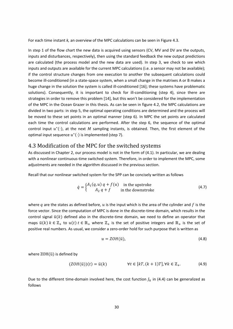
Figure 4.3: Flow chart for MPC calculations [14].
30
For each time instant k, an overview of the MPC calculations can be seen in Figure 4.3.
In step 1 of the flow chart the new data is acquired using sensors (CV, MV and DV are the outputs,
inputs and disturbances, respectively), then using the standard feedback the new output predictions
are calculated (the process model and the new data are used). In step 3, we check to see which
inputs and outputs are available for the current MPC calculations (i.e. a sensor may not be available);
if the control structure changes from one execution to another the subsequent calculations could
become ill-conditioned (in a state-space system, when a small change in the matrixes A or B makes a
huge change in the solution the system is called ill-conditioned [16]; these systems have problematic
solutions). Consequently, it is important to check for ill-conditioning (step 4), since there are
strategies in order to remove this problem [14], but this won’t be considered for the implementation
of the MPC in the Ocean Grazer in this thesis. As can be seen in figure 4.2, the MPC calculations are
divided in two parts: in step 5, the optimal operating conditions are determined and the process will
be moved to these set points in an optimal manner (step 6). In MPC the set points are calculated
each time the control calculations are performed. After the step 6, the sequence of the optimal
control input ( ), at the next sampling instants, is obtained. Then, the first element of the
optimal input sequence ( ) is implemented (step 7).
4.3 Modification of the MPC for the switched systems As discussed in Chapter 2, our process model is not in the form of (4.1). In particular, we are dealing
with a nonlinear continuous-time switched system. Therefore, in order to implement the MPC, some
adjustments are needed in the algorithm discussed in the previous section.
Recall that our nonlinear switched system for the SPP can be concisely written as follows
{ ( ) ( )
(4.7)
where are the states as defined before, is the input which is the area of the cylinder and is the
force vector. Since the computation of MPC is done in the discrete-time domain, which results in the
control signal ( ) defined also in the discrete-time domain, we need to define an operator that
maps ( ) to ( ) where is the set of positive integers and is the set of
positive real numbers. As usual, we consider a zero-order hold for such purpose that is written as
( ), (4.8)
where ( ) is defined by
( ( ))( ) ( ) [ ( ) ] . (4.9)
Due to the different time-domain involved here, the cost function in (4.4) can be generalized as
follows
31
( ) ∫ ( ( ) ( ) ( ( )⏟
) ( ) ( ( )⏟
)( ))
(4.10)
With the explained modifications, the MPC algorithm can be summarize as follows.
1- Set the initial time step .
2- Compute the optimal input [ ( ) ( ) ( )] that solves the following
optimization problem.
( ) (4.11)
subject to:
{
( ) ( )
(4.12)
( ) ,
where and are the lower and upper bounds for the state values.
3- Set the control input at time , ( ) ( ).
4- Increment and repeat from step 2.
4.4 Optimization problem
4.4.1 Introduction to the ICLOCS toolbox As was explained in the previous section, the MPC controller needs to solve an optimization problem
at every sampling instant. The software that is going to be used for the implementation of the MPC
is Matlab; in order to save time in coding, the utilization of one of the toolboxes available for
optimization problems was considered as an alternative.
The toolbox used in this work is the ICLOCS toolbox (Imperial College London Optimal Control
Software User). Other options were considered as well, but the choice of the ICLOCS toolbox was
made for different reasons. The ICLOCS toolbox allows users to define optimal control problems with
general path and boundary constraints, free or fixed final times and the ability to include constant
design parameters as unknowns. The different control problems that can be solved with this toolbox
are the following ones [17]:
( )
( ( ) ( ) ) (4.13)
subject to
( ( ) ( ) ) ( ) [ ]
( ( ) ( ) ) [ ]
( ) [ ] (4.14)
( ) [ ]
( ) [ ]
32
where is the cost function that we want to minimize.
The function ( ) describes general path constraints and ( ) imposes the boundary conditions at
the beginning and end of the phase.
As a first step, the optimal control problem defined by the user is transcribed to a static optimisation
problem by either direct multiple shooting or direct collocation methods (using a solver package like
CVODES). Once the optimal control problem has been transcribed it can be solved with a selection of
nonlinear constrained optimisation algorithms (different NLP solvers or the IPOPT solver can be used
[18]).
4.4.2 Choice of the cost function Recall that for our purposes, the cost function will depend on the distance between the buoy and
the wave and on the volume of water pumped (proportional to the amount of energy extracted). In
particular, we modify the cost function ( ) as in (4.9) into
( )
[ ]| ( ) ( )|
[ ]
( ) ( )
⏟
(4.15)
or
( ) ∫ | ( ) ( )|
[ ]
( ) ( )
⏟
(4.16)
where are positive weighting constants to be decided.
First, we determine the most suitable cost function to be used (i.e., (4.15) or (4.16)). Recall that we
want to minimize the distance between the buoy and the wave for guaranteeing that the buoy is
following the wave profile. The distance between the buoy and the wave can be calculated using the
L2 distance like in (4.15) or using the maximum distance between the buoy and the wave like in
(4.14).
In order to choose the cost function to be used, we run two simulations with the same wave profile
and initial conditions, but with different input. These simulations are shown in Figure 4.4 where for a
particular input we obtain a nice behaviour of the buoy (Figure 4.4a), while the other input results in
an undesirable buoy profile (Figure 4.4b). Using these simulations, we compute respectively the
distance ‖ ‖ and ‖ ‖ which are the main differences between (4.15) and (4.16).

33
Figure 4.4: Simulations for choosing the distance formulation
If the values of the maximum (or ‖ ‖ ) and the L2 distance (or ‖ ‖ ) between the
wave and the buoy are compared for both simulations, we obtain the following results: for the
simulation in the Figure 4.4 (a) ‖ ‖ , ‖ ‖ , and for the
simulation in the Figure 4.4 (b) ‖ ‖ , ‖ ‖ . The L2 distance
is smaller for the lower plot despite the behaviour of the buoy being clearly better for the upper
plot, since the buoy is shown to accurately track wave motion with consistent submersion. The
‖ ‖ is smaller for the simulation in the Figure 4.4 (a), where the buoy follows the wave
profile with accuracy. Minimizing the maximum distance between the buoy and the wave we
guarantee a nice behaviour of the buoy profile. The cost function that has been chosen is the
following:
( )
[ ]| ( ) ( )|
[ ]
( ) ( )
⏟
(4.17)
The weights and play an important role in determining which component is more important
for desirable behaviour of the closed-loop system. In order to choose the weight values for
each term of the cost function, we evaluate the variation of ( ) as a function of the input as given in
Table 4.1. The table is based on simulation setup using the same initial conditions and a wave weight
of 4 meters.
Ac (m2) ‖ ‖ (m) Vpumped (m3)
0.06 0.9251 0.2397
0.12 0.9443 0.4801
0.18 0.9496 0.7365
0.24 0.9640 0.9789
0.30 0.9806 1.1873
Table 4.1: Values of the volume pumped and maximum distance between the wave and the buoy for different cylinder areas.
The variation between the best and worst result of the maximum distance between the buoy and
the wave is much smaller than the variation between the best and worst result of pumped volume.

34
Therefore it is decided to multiply the distance by a factor of 20 in the cost function. Notice that, as a
result of minimizing the cost function ( ), the is maximized.
The chosen weights are
.
(4.18)
Beyond maximizing the amount of energy extracted from the waves, we need to ensure that the
system behaves predictably, enabling the accurate tracking of wave motion by the buoy-piston
system. For this reason, the distance between the buoy (COM) and the wave (surface) has to be
considered in the cost function.
The cost function ( ) that used in this thesis is defined as follows:
( )
[ ]| ( ) ( )|
[ ]
( ) ( )
⏟
(4.19)
4.4.3 Implementation of the SPP model into ICLOCS The ICLOCS toolbox allows the user to solve huge optimization problems [17]; in this work the
problem to be solved is not an easy one (it is important to remember that in the dynamical model 6
state variables are used and the SPP is defined as a switched system).
Nevertheless, this toolbox has been chosen because of the different possibilities during the
definition of the optimization problem. First of all, due to different reasons (e.g., to ensure that the
piston can move only within a prescribed stroke within its cylinder) it is very important for the wave
energy converter to define boundaries for the state variables. The values for the different
boundaries have been chosen with the aim to protect all the WEC components from structural
damage (Table 4.2).
State variable Lower boundary Upper boundary
x1 (m) 130 150
v1 (m/s) -10 10
x2 (m) -10 10
v2 (m/s) -7 7
p1 (Pa) - -
p4 (Pa) - -
Table 4.2: Boundaries for the state variables.
The boundary values reported in Table 4.2 were obtained by running simulations of the SPP model
for the extreme case of 20-m high waves . Taking into account that a wave of 20 metres in height is a
very large wave, using the boundaries of the Table 4.2 for the state variables we ensure that the
components of the WEC are not going to be damaged by introducing buffers to preclude
catastrophic contact. Furthermore, as shown in the Table 4.2, no boundaries have been included for
the pressures in the upper and the lower reservoir; it is obvious that in the real system there will be
boundaries for these state variables. The reason we do not consider these pressures as bounded for
35
the present work is that the emptying of the upper reservoir to the lower reservoir through the
turbine it is not included in the dynamical model, which means that the amount of water in the
upper reservoir (proportional to the pressure) will always increase (upstroke) or remain constant
(downstroke), while for the lower reservoir the pressure will always decrease (upstroke) or remain
constant (downstroke).
The boundaries of the state variables should be included in the definition of the optimization
problem as they have to be respected. With the inclusion of the boundaries, the time needed for the
toolbox to solve this optimization problem will increase (the boundaries of all the state variables
have to be checked in each iteration).
The toolbox provides different functions and scripts that are used during the solution of the
optimization problem. The script for the definition of the optimization problem for the Ocean Grazer
can be found in the Appendix A.2, while the other scripts used can be found in [17].
Cost function
The cost function has the following form in the toolbox:
( ( ) ( ) ) ∫ ( ( ) ( ) )
( ) (4.20)
where E(·) is the cost associated with the boundary conditions and L(·) the stage cost function. The arguments over which the cost function can be minimised are the time-varying control input signals u(·), the initial state x0, the final time tf and a set of parameters p that are constant for the duration of the phase. For the cost function chosen above, it is only necessary to use the stage cost term (the boundary
cost will be equal to 0). The formulation of the cost function can be found in Appendix A.2.
Definition of the ODEs
As it was explained before, the single-piston pump (SPP) dynamical model is a switching system. It is
important to know that the ICLOCS toolbox was not designed for switching systems [17].
Furthermore, the toolbox treats the control input as a continuous variable but the area of the
cylinder takes discrete values. To solve this problem the control input has been rounded down to
the previous integer number; hence, despite the toolbox treating the control input as a continuous
variable, it will be applied as a discrete one to the ODE equations. The control input is the area of the
piston so, in the ODEs the area of the piston has been replaced by the following expression:
⌊ ⌋ (4.21)
By connecting 3 pistons to each buoy, we are able to simulate 7 different effective radii for the
pistons (which means 7 different effective piston areas) as is explained in detail in [19].
Therefore we set up the lower boundary equal to 1 and the upper one equal to 7 for the control
input so the different available areas will be:
36
Control Input (u) Ac (m2)
1 0.06
2 0.12
3 0.18
4 0.24
5 0.30
6 0.36
7 0.42
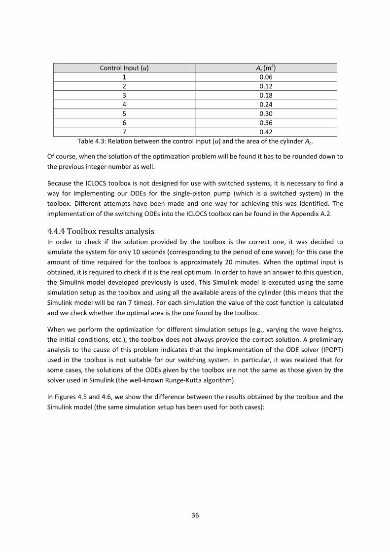
Table 4.3: Relation between the control input (u) and the area of the cylinder Ac.
Of course, when the solution of the optimization problem will be found it has to be rounded down to
the previous integer number as well.
Because the ICLOCS toolbox is not designed for use with switched systems, it is necessary to find a
way for implementing our ODEs for the single-piston pump (which is a switched system) in the
toolbox. Different attempts have been made and one way for achieving this was identified. The
implementation of the switching ODEs into the ICLOCS toolbox can be found in the Appendix A.2.
4.4.4 Toolbox results analysis In order to check if the solution provided by the toolbox is the correct one, it was decided to
simulate the system for only 10 seconds (corresponding to the period of one wave); for this case the
amount of time required for the toolbox is approximately 20 minutes. When the optimal input is
obtained, it is required to check if it is the real optimum. In order to have an answer to this question,
the Simulink model developed previously is used. This Simulink model is executed using the same
simulation setup as the toolbox and using all the available areas of the cylinder (this means that the
Simulink model will be ran 7 times). For each simulation the value of the cost function is calculated
and we check whether the optimal area is the one found by the toolbox.
When we perform the optimization for different simulation setups (e.g., varying the wave heights,
the initial conditions, etc.), the toolbox does not always provide the correct solution. A preliminary
analysis to the cause of this problem indicates that the implementation of the ODE solver (IPOPT)
used in the toolbox is not suitable for our switching system. In particular, it was realized that for
some cases, the solutions of the ODEs given by the toolbox are not the same as those given by the
solver used in Simulink (the well-known Runge-Kutta algorithm).
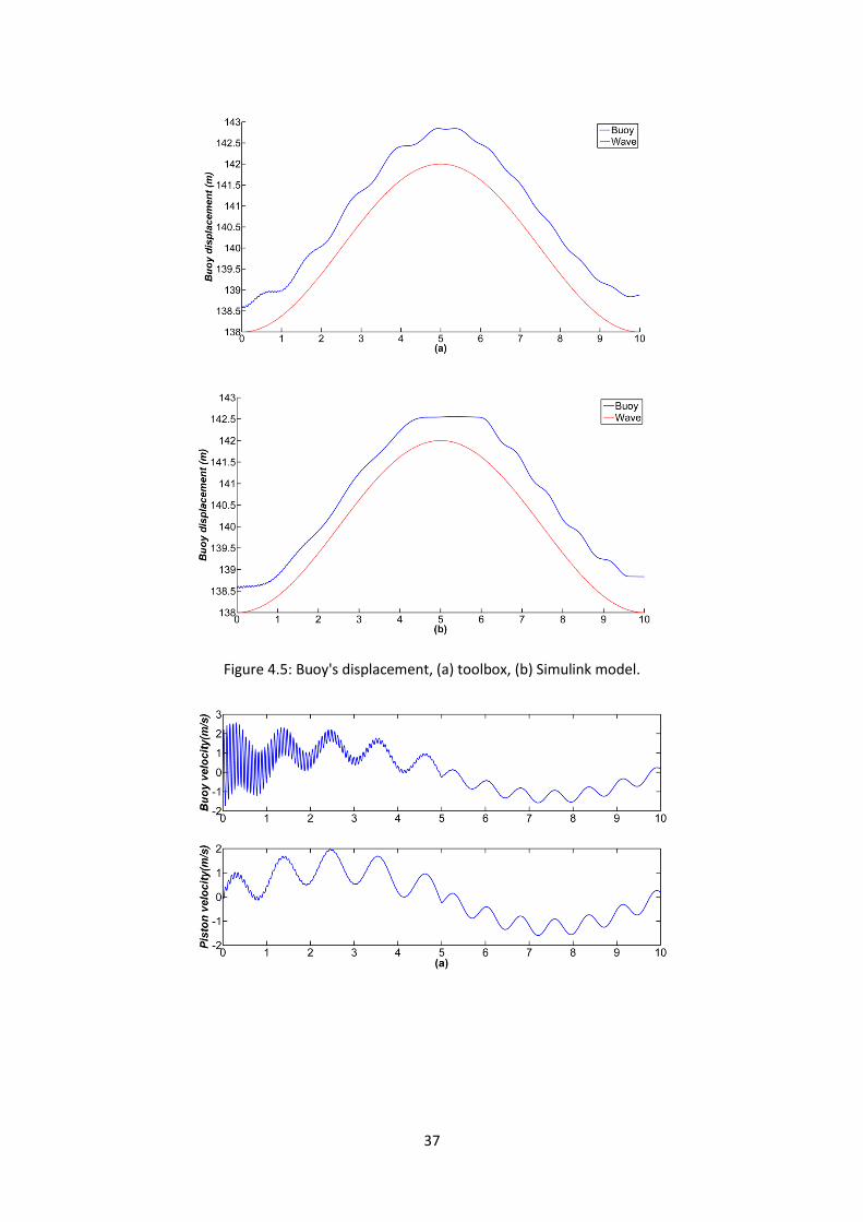
In Figures 4.5 and 4.6, we show the difference between the results obtained by the toolbox and the
Simulink model (the same simulation setup has been used for both cases):
37
Figure 4.5: Buoy's displacement, (a) toolbox, (b) Simulink model.

38
Figure 4.6: Buoy's and piston's velocity, (a) toolbox, (b) Simulink model.
Since solving the optimization problem in (4.11) is a crucial step in the MPC algorithm, the use of
ICLOCS toolbox is currently not applicable in our MPC algorithm. However, this toolbox remains an
interesting tool for future development provided that the aforementioned problems have been
resolved. Due to the unavailability of an optimzation solver for (4.11), we resort to an exhaustive
search that is achievable for short time horizon, as detailed in the followint subsection.
4.4.5 Exhaustive search Another way to solve the optimization problem is to perform an exhaustive search of all possible
combinations. Recall that in our MPC algorithm, we need to solve the following optimization
problem:
( ) (4.22)
subject to:
{
( ) ( )
(4.23)
( ) ,
where and are the lower and upper bounds for the state values.
Finding the optimal input [ ( ) ( ) ( )] amounts to searching the space of
combinations [ ( ) ( ) ( )] from the input space. For instance, if the input space is
a discrete set of values, then the number of input combinations is where is the control
horizon (the number of waves that will be considered). Therefore for small and , it is feasible for
us to obtain explicitly the solution within a reasonable amount of simulation time.
In order to obtain the optimal sequence of areas with the exhaustive search, the Simulink model of
the single-piston pump (SPP) is going to be used. Simulations with all the combinations of the
available piston areas ( ) for the considered number of waves ( , which is not a fixed value) will be
done and the value of the cost function ( ) is calculated for each case. A program for this

39
exhaustive search has been developed and is called ‘Running all combinations’; its code can be
found in the Appendix A.3.2.
Due to the number of combinations increases exponentially depending on the number of available
cylinder areas, the number of available cylinder areas is fixed at , the selected discrete values
of the areas are 0.06 m2, 0.18 m2 and 0.30 m2.
For all the simulations the integration step size is 10-3; with this step size, the convergence in the
Runge Kutta algorithm is guaranteed and the precision in the obtained solutions of the ODE
equations is high (the results doesn’t change using an integration step size of 10-4).
4.5 Implementation of the MPC After having discussed the modified MPC algorithm in section 4.2, where the exhaustive search will
be used to solve the optimization step, we will evaluate the performance of MPC for our system.
As an initial simulation setup for this evaluation, we consider a wave profile with varying height as
shown in Figure 4.7 (the height values are, consecutively 6, 2, 12, 8, 4 and 10 meters). For the input,
we consider only three different cylinder areas (due to the reason explained in subsection 4.4.5). For
the MPC algorithm, we consider the time horizon of where is the wave period. Note
that in this case the optimization step will involve the finding of optimal input sequences
( ) ( ) and ( ).
Figure 4.7: Input wave (displacement measured from the piston’s centre of mass).
In order to better understand the working principle of the MPC controller, we discuss the
implementation of the algorithm for the first few steps as follows.
During the first step, the algorithm will consider the waves of 6, 2 and 12 meters and the
optimization step will give the optimal input sequence for these waves. At the end of the first step,
the algorithm applies the first solution (the first obtained area). Then, after applying the first optimal
solution, and when the wave of 6 meters height has already acted on the system, then the algorithm
is repeated and it will consider the waves of 2, 12 and 8 meters.
At this time the algorithm will get the optimal sequence of 3 areas for these three waves and but will
only apply the first one. This algorithm is repeated again for the subsequent waves.
40
For the implementation of the MPC in the developed dynamical model of the SPP, we use 2 different
Simulink models. One model (Model A) is used to simulate the actual system (the plant). The other
model (model B) will be used as the prediction model used by the MPC algorithm for solving the
optimization problem (4.11).
The sequence of actions for the implementation and execution of the MPC algorithm is as follows (6
waves input described above is assumed):
1 – The algorithm calculates the optimal input sequence (considering the waves of 6, 2 and 12
meters). Only the first element of the obtained sequence (which is the cylinder area for the wave of
6 meters) is implemented to the plant. Model B is used.
2 – With the obtained cylinder area in point 1, the plant is simulated until the end of the 6 meters
wave, when the simulation is paused. Model A is used.
3 –Considering the current conditions of the plant (the final value of the state variables in point 2),
the algorithm calculates the optimal input sequence for the waves of 2, 12 and 8 meters. Only the
first element of the obtained input sequence (which is the cylinder area for the wave of 2 meters) is
implemented to the plant. Model B is used.
4 - The simulation of point 2 is restarted using the area value obtained in step 3. Model A is used.
5 –The sequence is repeated for the other waves.
The developed program for the implementation of the MPC can be found in the Appendix A.3.3
along with detailed explanations of the changes made for the 2 models used (compared with the
Simulink model used for the initial simulations without any control).
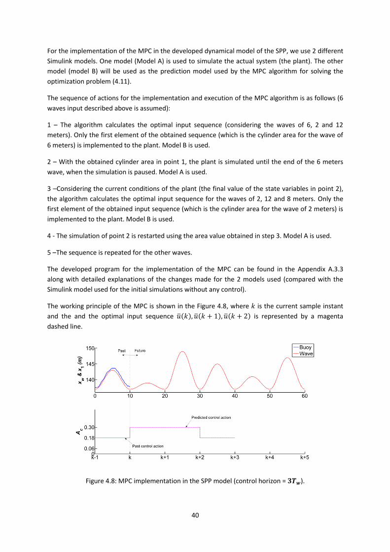
The working principle of the MPC is shown in the Figure 4.8, where is the current sample instant
and the and the optimal input sequence ( ) ( ) ( ) is represented by a magenta
dashed line.
Figure 4.8: MPC implementation in the SPP model (control horizon = ).

41
4.6 Lookup table as an alternative control strategy A lookup table is a simple control strategy that consists of finding the optimal cylinder area for each
kind of wave. With this information stored as a database, and depending on the incoming wave, the
optimal area of the cylinder will be chosen by looking-up the appropriate value from the database.
The main advantage of the usage of the lookup table is that the time needed for applying the control
is practically insignificant.
In order to build the lookup table for our simulation, and since we will consider combinations of
waves with the height of 2, 6, 8, and 12 meters, we run simulations for every wave and for every
area of cylinder (we have considered 5 different cylinder areas: 0.06, 0.12, 0.18, 0.24 and 0.30 m2).
These simulation results are given in Table 4.4 – 4.7 where we use the cost function
( )
[ ]| ( ) ( )|
[ ]
( ) ( )
⏟
(4.24)
as discussed in the section 4.4.2.
In these tables, the optimal input for every different wave is highlighted in bold.
Ac (m2) J
0.06 17.9098
0.12 18.0839
0.18 18.0355
0.24 18.0732
0.30 18.0211
Table 4.4: Results values for Hw=2.
Ac (m2) J
0.06 18.5647
0.12 18.5779
0.18 18.3017
0.24 18.2619
0.30 18.5678
Table 4.5: Results values for Hw=6.
Ac (m2) J
0.06 18.8113
0.12 18.6248
0.18 18.2141
0.24 18.0733
0.30 18.6788
Table 4.6: Results values for Hw=8.
Ac (m2) J
0.06 19.1727
0.12 18.6307
0.18 17.8525
0.24 17.4871
0.30 18.9903
Table 4.7: Results values for Hw=12.

42
Based on these simulations, the resulting lookup table is shown in Figure 4.9.
Figure 4.9: Lookup table.
Knowing the optimal solution for each type of wave (according to height and period) does not mean
that in a more realistic simulation (where the input can be a sequence of waves with different
profiles) the optimal solution will be the same. Instead, real-time measurements of incoming waves
and operating parameters will be necessary for active system control.
Let us now apply the lookup table control strategy to the simulation setup considered in the
previous section. In this case, the input that is implemented at each step is obtained from the lookup
table (Figure 4.9). The code of the program used in these calculations can be found in Appendix A.3.
The result is shown in Figure 4.10 (c.f. Figure 4.8 for the MPC one).
Figure 4.10: Simulation results obtained applying the lookup table.

43
In this case, the pumped volume value for the 40 seconds of simulation (after four waves) is
calculated in the same way as explained in the equation 4.13 and has a value of 6.186 m3, while the
value of the maximum distance between the buoy and the sea level is 1.034 m. Thus, the objective
function J value for this case is 14.505.
In order to compare these results with the optimal input combination and with the results obtained
by applying the MPC, the number of available cylinder areas will be reduced from 5 to 3 (0.06, 0.18
and 0.30 m2). If only these 3 areas are considered, the lookup table results are changed and the
optimal solution obtained for the lookup table will be 0.06 m2 for the wave of 2 metres height, 0.18
m2 for the wave of 6 metres height, 0.18 m2 for the wave of 8 metres height and 0.18 m2 for the
wave of 12 metres height. The comparison of results between the optimal control input, the MPC
and the lookup table results is presented in the following section.
4.7 Results analysis
4.7.1 Comparison of Controller results In this section, we will compare the performance of the MPC with and , and of
the lookup table strategy. We will also compare these results with the optimal input (obtained by
the exhaustive search).
One would think that a controller would be unnecessary if there was a possibility of finding the optimum solution beforehand. However, it is necessary to keep in mind the theory behind the MPC explained on the section 4.2, where it was explained that obtaining the real optimal solution for will be only possible if there is a perfect match between the model and the plant and there were no disturbances. For all the simulations below, the dynamical model developed (section 2.2) is used as the real SPP; hence, the controller is necessary because there will always mismatch between the model and the plant. In the following results, we still consider the simulation setup as given in section 4.5.
( ) ( ) ( ) ( ) J Vpumped (m3)
‖ ‖ (m)
tsim(hours)
0.30 0.30 0.30 0.30 13.5639 7.9488 1.0756 15
Table 4.8: Results for the optimal sequence of cylinder areas.
( ) ( ) ( ) ( ) J Vpumped (m3)
‖ ‖ (m)
tsim(min)
0.06 0.30 0.18 0.18 14.4587 4.3926 0.9426 25
Table 4.9: Results obtained by the MPC (control horizon ).
( ) ( ) ( ) ( ) J Vpumped (m3)
‖ ‖ (m)
tsim(hours)
0.18 0.30 0.18 0.30 14.0941 6.0173 1.0056 2
Table 4.10: Results obtained by the MPC (control horizon ).
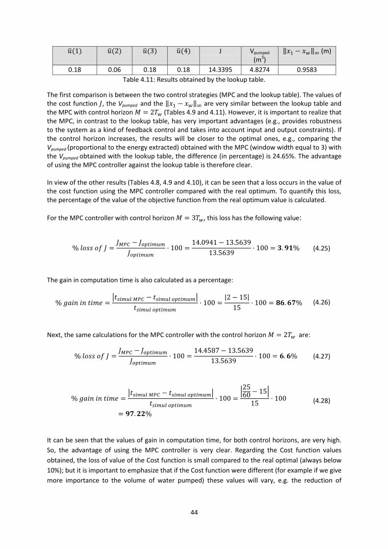
44
( ) ( ) ( ) ( ) J Vpumped (m3)
‖ ‖ (m)
0.18 0.06 0.18 0.18 14.3395 4.8274 0.9583
Table 4.11: Results obtained by the lookup table.
The first comparison is between the two control strategies (MPC and the lookup table). The values of the cost function , the Vpumped and the ‖ ‖ are very similar between the lookup table and the MPC with control horizon (Tables 4.9 and 4.11). However, it is important to realize that the MPC, in contrast to the lookup table, has very important advantages (e.g., provides robustness to the system as a kind of feedback control and takes into account input and output constraints). If the control horizon increases, the results will be closer to the optimal ones, e.g., comparing the Vpumped (proportional to the energy extracted) obtained with the MPC (window width equal to 3) with the Vpumped obtained with the lookup table, the difference (in percentage) is 24.65%. The advantage of using the MPC controller against the lookup table is therefore clear. In view of the other results (Tables 4.8, 4.9 and 4.10), it can be seen that a loss occurs in the value of the cost function using the MPC controller compared with the real optimum. To quantify this loss, the percentage of the value of the objective function from the real optimum value is calculated.
For the MPC controller with control horizon , this loss has the following value:
(4.25)
The gain in computation time is also calculated as a percentage:
| |
| |
(4.26)
Next, the same calculations for the MPC controller with the control horizon are:
(4.27)
| |
| |
(4.28)
It can be seen that the values of gain in computation time, for both control horizons, are very high.
So, the advantage of using the MPC controller is very clear. Regarding the Cost function values
obtained, the loss of value of the Cost function is small compared to the real optimal (always below
10%); but it is important to emphasize that if the Cost function were different (for example if we give
more importance to the volume of water pumped) these values will vary, e.g. the reduction of

45
volume pumped obtained with the controller (control horizon ) with respect to the real
optimum is 24.3%.
According to the results, the advantage of using this controller is clear. However, the boundaries of
the state variables should not be violated since it is part of the MPC algorithm. Next, the maximum
and minimum values for all state variables are shown.
State variable Min. Value Max. Value Lower boundary Upper boundary
x1(m) 137.559 149.922 130 150
v1(m/s) -4.0163 5.0802 -10 10
x2(m) -2.4415 9.9179 -10 10
v2(m/s) -4.0322 5.1760 -7 7
p1(Pa) 196200 1.9708e+05 - -
p4(Pa) 1.9532e+05 196200 - -
Table 4.12: Values of state variables for the MPC results ( )
In order to verify that the results obtained are generally applicable, the simulation setup is modified.
In this case, we use a wave sequence with the following heights: 12, 6, 2, 4, 8 and 5 meters.
Figure 4.11: Alternative input wave (displacement measured from the piston’s centre of mass).
The results are shown in the Tables 4.13, 4.14 and 4.15.
( ) ( ) ( ) ( ) J Vpumped (m3)
| ( | (m)
tsim(hours)
0.18 0.30 0.30 0.30 14.1642 5.4094 0.9787 15
Table 4.13: Results for the optimal sequence of cylinder areas.
( ) ( ) ( ) ( ) J Vpumped (m3)
| ( |(m)
tsim(min)
0.18 0.18 0.30 0.30 14.6274 4.7929 0.9710 25
Table 4.14: Results obtained by the MPC (control horizon ).
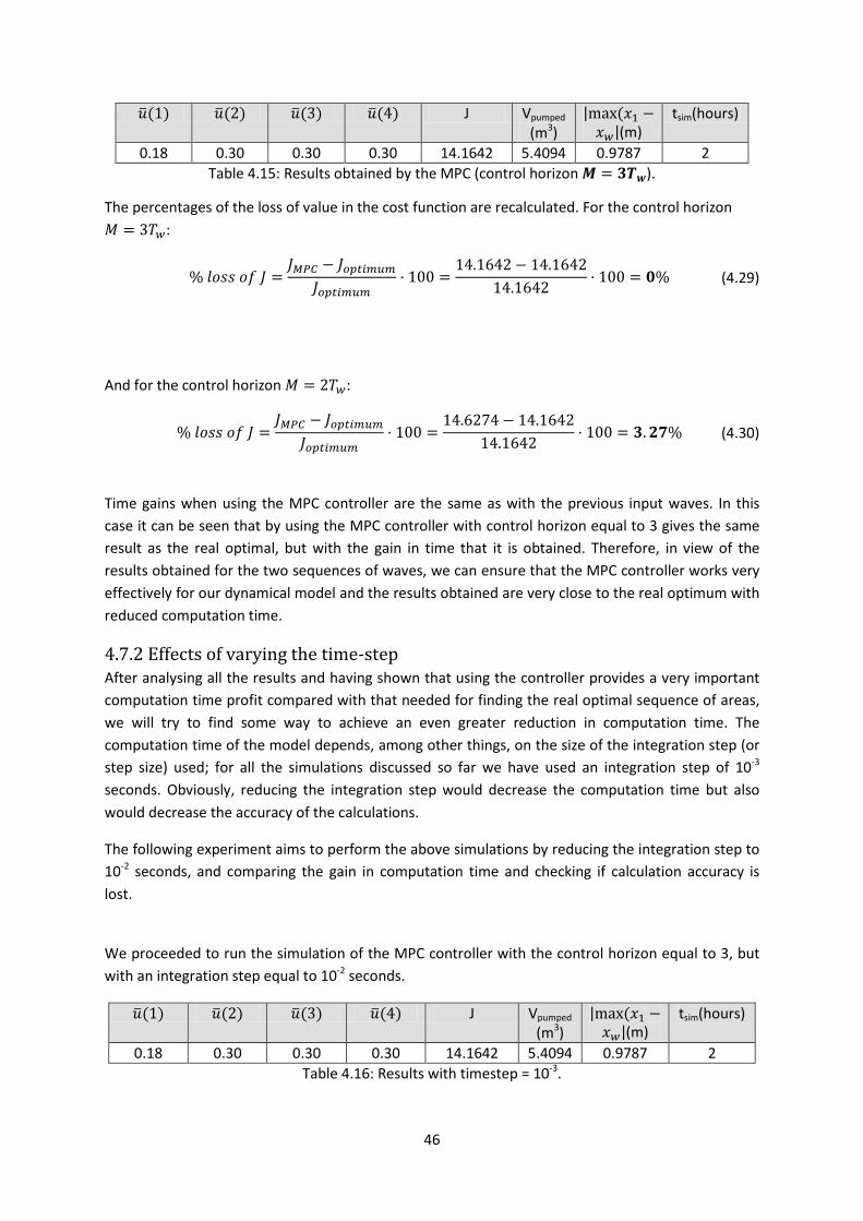
46
( ) ( ) ( ) ( ) J Vpumped (m3)
| ( |(m)
tsim(hours)
0.18 0.30 0.30 0.30 14.1642 5.4094 0.9787 2
Table 4.15: Results obtained by the MPC (control horizon ).
The percentages of the loss of value in the cost function are recalculated. For the control horizon
:
(4.29)
And for the control horizon :
(4.30)
Time gains when using the MPC controller are the same as with the previous input waves. In this
case it can be seen that by using the MPC controller with control horizon equal to 3 gives the same
result as the real optimal, but with the gain in time that it is obtained. Therefore, in view of the
results obtained for the two sequences of waves, we can ensure that the MPC controller works very
effectively for our dynamical model and the results obtained are very close to the real optimum with
reduced computation time.
4.7.2 Effects of varying the time-step After analysing all the results and having shown that using the controller provides a very important
computation time profit compared with that needed for finding the real optimal sequence of areas,
we will try to find some way to achieve an even greater reduction in computation time. The
computation time of the model depends, among other things, on the size of the integration step (or
step size) used; for all the simulations discussed so far we have used an integration step of 10-3
seconds. Obviously, reducing the integration step would decrease the computation time but also
would decrease the accuracy of the calculations.
The following experiment aims to perform the above simulations by reducing the integration step to
10-2 seconds, and comparing the gain in computation time and checking if calculation accuracy is
lost.
We proceeded to run the simulation of the MPC controller with the control horizon equal to 3, but
with an integration step equal to 10-2 seconds.
( ) ( ) ( ) ( ) J Vpumped (m3)
| ( |(m)
tsim(hours)
0.18 0.30 0.30 0.30 14.1642 5.4094 0.9787 2
Table 4.16: Results with timestep = 10-3.

47
( ) ( ) ( ) ( ) J Vpumped (m3)
| ( |(m)
tsim(min)
0.18 0.30 0.30 0.30 14.0169 5.4789 0.9748 12
Table 4.17: Results with timestep = 10-2.
In view of the results, the time savings are very significant:
| |
| |
(4.31)
As shown above, the sequence of areas obtained is exactly the same as using the integration step of
10-3 seconds. Obviously, the volume of water pumped and the maximum distance between buoy and
wave are not exactly the same as using the integration step 10-3 seconds, as expected.
In view of these results, one might think that we will always get the same sequence of areas with the
integration step of 10-2 seconds as well as using an integration step of 10-3 seconds. However, this
will not happen all the time. Depending to the importance given to the computation time saved,
some loss in the precision of the results can be tolerated. The clear conclusion is that reducing the
integration step to 10-2 seconds is an option that should be considered and studied in depth.
4.7.3 Comparison using or not MPC controller In order to complete the part of the control applied to the wave energy converter, it is useful to
compare the results obtained with and without the application of the control strategy discussed
above. The purpose of this comparison is to demonstrate the importance of control, and show the
usefulness of the content of this work.
This comparison is done using exactly the same simulation setup. In the first case, the sequence of
cylinder areas found by the MPC controller is applied; and in the other case, an average (constant)
area of 0.18m2 is applied instead. The comparison is carried out with the 2 sequences of 6 waves
used in previous experiments in order to obtain a comparable result.
In Tables 4.18 - 4.21, the comparison results of the cost function values, the pumped water volume
and the maximum distance between buoy and wave, are shown:
( ) ( ) ( ) ( ) J Vpumped (m3)
| ( |(m)
0.18 0.30 0.18 0.30 14.0941 6.0173 1.0056
Table 4.18: Results with MPC controller (input waves: 6,2,12 and 8 meters height).

48
( ) ( ) ( ) ( ) J Vpumped (m3)
| ( |(m)
0.18 0.18 0.18 0.18 14.1561 5.0108 0.9583
Table 4.19: Results without using any controller (input waves: 6,2,12 and 8 meters height).
( ) ( ) ( ) ( ) J Vpumped (m3)
| ( |(m)
0.18 0.30 0.30 0.30 14.1642 5.4094 0.9787
Table 4.20: Results with MPC controller (input waves: 12,6,2 and 4 meters height).
( ) ( ) ( ) ( ) J Vpumped (m3)
| ( |(m)
0.18 0.18 0.18 0.18 15.1968 4.2236 0.9710
Table 4.21: Results without using any controller (input waves: 12,6,2 and 4 meters height).
From the results obtained it appears that the use of the MPC controller does not affect the good
performance of the system for these waves (the maximum difference between the wave and the
buoy practically no varies.). However, there is a significant difference in the pumped water volume,
which is higher using the MPC controller.
Considering that the water volume will fall from the upper tank to the lower tank through a turbine
(and thus will generate electricity), the pumped water volume is directly related to the energy
extracted from the waves. Assuming a turbine efficiency of 0.9 [20] and an electric generator
efficiency of 0.95, the electric power obtained from the hydro turbine has the following formulation
[21]:
(4.32)
where is the time needed for the amount of water for going from the upper to the lower
reservoir (in seconds), is the cylinder length in meters, and are the turbine
and generator yields respectively.
Because it is unknown how the water will be transported from the upper reservoir to the lower
reservoir, the time is unknown, so that instead of comparing the generated electric power,
the electric energy generated is compared:
(4.33)
In tables 4.22 and 4.23, results of extracted wave energy system, with and without controller, are
shown:

49
MPC controller Vpumped (m3) Eelec (KJ)
No 5.0108 4202.83
Yes 6.0173 5047.04
Table 4.22: Energy results for wave sequence 6,2,12 and 8 metres.
MPC controller Vpumped (m3) Eelec (KJ)
No 4.2236 3542.56
Yes 5.4094 4537.16
Table 4.23: Energy results for wave sequence 12, 6, 2 and 4 metres.
As can be seen in both cases, the difference between the energy extracted from the waves with or
without the controller is about 1000 KJ (for the wave used in the Table 4.22). Not using the
controller causes a loss of 20% in the extracted energy, while for the waves used in Table 4.23 the
extracted energy loss due to not using the controller is 28%.
As shown by the latter simulations, the importance of using the MPC controller for selecting the
right piston area as a function of the incoming waves has been demonstrated.
The main goal of control has been achieved within this context: maximizing the amount of energy
extracted from the ocean waves. It is important to make clear that the implementation of the MPC
that has done in this work is an initial step in the control of the Ocean Grazer. In the simulations, the
real plant (the WEC) has been substituted by the dynamical model, so the next step could be use the
developed scaled prototype as the plant of the system which will provide much more reliable
results.
4.7.4 Comparison with a significant number of input waves. In the previous sections, only two different input waves have been used for the simulations and for
comparing the results. However, in order to demonstrate if the behaviour of the MPC is consistent
with that of the previous sections for a significant number of different waves, many more
simulations should be performed.
In this section, 50 different sequences of 6 waves (obtained randomly, using waves ranging in height
from 1 to 12 meters [4]) have been used for comparing the results between the optimal solution
(using the exhaustive search), the WEC with the MPC and the results without any controller.
Recall that the integration step size that has been used for all the previous simulations is 10-3. With
this integration step size, and only for calculating the optimal solution for the 50 different input
sequences, the needed simulation time is , which is not a
reasonable simulation time for us. Because of this, the integration step size has been reduced to 10-2
for the following simulations, and a small loss of accuracy in the solutions of the ODE equations has
been assumed.

50
Figure 4.12: Comparison of the Cost function value.
Figure 4.13: Comparison of the energy extracted.
In Figure 4.12, the value of the cost function (equation 4.18) is compared. Recall that in the
optimization problem (section 4.3), the cost function is to be minimized. As can be seen in Figure
4.12, the optimal value for the cost function is achieved most of the time by the MPC controller. In
these simulations the window width that has been used for the MPC controller is equal to 3 and, if
its value is increased, the results will be more close to the optimal ones so we can conclude that the
MPC controller guarantees results very close to the optimal ones.
In Figure 4.13, a comparison of the energy extracted (equation 4.28) is shown. The fact that the MPC
achieves the optimal results most of the time can be seen in this plot as well, but the most important
fact is the comparison with the results not using the MPC controller. The loss in the energy extracted
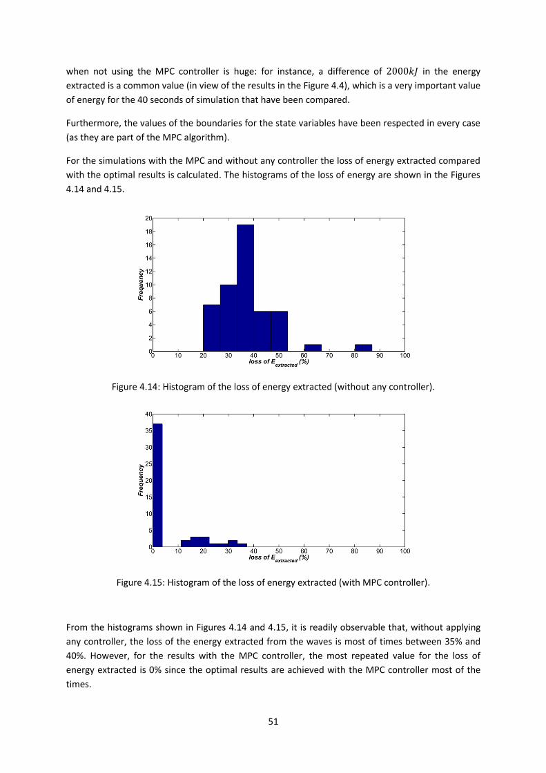
51
when not using the MPC controller is huge: for instance, a difference of in the energy
extracted is a common value (in view of the results in the Figure 4.4), which is a very important value
of energy for the 40 seconds of simulation that have been compared.
Furthermore, the values of the boundaries for the state variables have been respected in every case
(as they are part of the MPC algorithm).
For the simulations with the MPC and without any controller the loss of energy extracted compared
with the optimal results is calculated. The histograms of the loss of energy are shown in the Figures
4.14 and 4.15.
Figure 4.14: Histogram of the loss of energy extracted (without any controller).
Figure 4.15: Histogram of the loss of energy extracted (with MPC controller).
From the histograms shown in Figures 4.14 and 4.15, it is readily observable that, without applying
any controller, the loss of the energy extracted from the waves is most of times between 35% and
40%. However, for the results with the MPC controller, the most repeated value for the loss of
energy extracted is 0% since the optimal results are achieved with the MPC controller most of the
times.

52
The simulations that have been done in this section allow us to conclude the following points
regarding the MPC controller applied to the Ocean Grazer:
- The sequence of piston’s cylinder areas obtained is, most of time, the optimal one.
- The amount of energy extracted from the waves is maximized.
- Using the MPC controller we obtain an average gain of 40% in the energy extracted from the
waves.
- The boundaries for the state variables are not violated.

53
Chapter 5
Conclusions & Future work
During this thesis the mathematical model of the single-piston pump developed in [8] has been
improved. This developed model has been used to determine the influence of other variables in the
efficiency of the system via the analysis of variance (ANOVA), where the cylinder area is chosen as
the optimal control variable. Besides, the MPC has been chosen as the most suitable control strategy
for maximizing the amount of energy extracted by this WEC. The MPC algorithm has been adjusted
to our switched system and has been implemented in the developed model. The loss of energy
extracted (compared with the optimal solution) by applying the MPC algorithm is most of the times
equal to 0%, which means that the MPC algorithm achieves the optimal solution in almost all cases.
The first steps in the control field for the MP2PTO have been taken, but regarding this field there is
still further work to be done:
1- Combine the model of the SPP used in this thesis (with the implementation of the MPC) with
the new dynamical model that is being developed in [4].
2- Use the full-scale prototype as the plant of the system (there is always more or less
mismatch between a model and the real plant) and apply the MPC to this developed
prototype.
3- Further investigations on the piston choice mechanism for the Ocean Grazer (develop the
dynamical model for the multi-piston pump).
4- Solve the optimization problem of the MPC algorithm with a more efficient method, e.g.
solving the aforementioned problems with the ICLOCS toolbox.

54
Appendix A
This appendix includes all figures related with the code and the Simulink Matlab models that have
been used in the development of this thesis.
A.1 Dynamical Model As it was mentioned during the explanation of the simulation setup of the dynamical model, the
following dynamical model has been built in order to be easily understandable by someone else in
the future.
Figure A.1: Simulink model of the single piston-pump.
In the figure A.1 the comprehensive Simulink model is shown, where the input for the model (the
sine wave) and the formulation of the buoyancy force Fb is included. For the formulation of the
buoyancy fore Fb the following m-file is used.
Inside the ‘Single Piston Pump equations’ block there are three different subsystems, one for the
equations of the buoy (figure A.2), another one for the equations of the piston (figure A.4), and
another one for the equations of the pressure of the upper and lower reservoir (figure A.6).

55
Figure A.2: Subsystem for the buoy's equation.
Inside the ‘buoy’s equation’ subsystem the equations of motion for the buoy have been
implemented using Simulink blocks.
Figure A.3: Equations of motion for the buoy.
For the piston’s equation the subsystem of figure A.4 has been used.
Figure A.4: Subsystem for piston's equations.

56
The equations of motion for the piston have been implemented using a Matlab Function block with
the following code:
The fluid system has been implemented using only the velocity of the piston as the input for the
subsystem (the only state space variable that is needed for the equations of the fluid system).
Figure A.5: Fluid system.
Inside the ‘Fluid system’ block the implementation of the equations has been done.

57
Figure A.6: Inside Fluid System block.
The content of the Matlab Function used for the calculation of the flow rate is the following one:
The difference between the equations of pressure for the upper reservoir or the lower reservoir is
just a sign, so only the implementation of the equation for the upper reservoir will be shown in
figure A.7.
Figure A.7: Implementation of the equation for the pressure of the upper reservoir.
Using different subsystems allows different users to identify very quickly where each part of the
dynamical model is implemented; user friendliness was one of the objectives in building this
Simulink model.
In future work, when someone else improves the dynamical model, this Simulink model can be the
starting point for the improved model.

58
A.2 ICLOCS toolbox setup In the script ‘testProblem.m’ (which is included at the end of this section A.2) the definition of the
problem has to be implemented. As was explained before, it is also possible to define boundaries for
the state variables and for the control input, while the cost function and the ODEs of the model have
to be included in this script as well.
All the content of the script ‘testProblem.m’ is explained and justified in the following lines.
The initial time for the simulation t0 is equal to 0 and the final time, as was explained before, will be
tf=30. It is also important to define the initial conditions for the system; the initial conditions will be
the same as those explained in the description of the model. The next step is to define the state
bounds (table 4.2). It is also possible to define terminal state bounds but for the moment this option
won’t be used.
If the initial and final values of the state variables are known, the calculation time will be reduced if
we define these values in the variable ‘guess.states’. Otherwise, if the variable ‘guess.states’ is an
empty matrix, the initial trajectories will be generated by linearly interpolating between random (but
feasible) initial and final values for each state.
In this case, the simulation time will be 30 seconds, and during this time 3 waves (the period of each
wave is 10 seconds) will be used as inputs to the system. During these 30 seconds of simulation, we
want to obtain an optimal sequence of 3 areas of the piston (one for each wave) and, because of
this, the variable ‘inputs.N’ (N is the number of control actions) will be equal to 3.
It is known that the control input will be the area of the piston, but as is explained in [19], with 3
pistons available it is only possible to choose between 7 effective areas of the piston. Besides the
possibility of defining boundaries for the control input, the control input is treated in the toolbox as
a continuous variable. However, the area of the piston is a discrete variable with only 7 different
values. The way to implement this issue in the toolbox will be explained when the ODEs of the
toolbox will be defined, but first it is important to define the boundaries for the control input: the
lower boundary will be 1 and the upper boundary 7 (the reason for this will be explained later).
Different parameters that will be needed for the cost function and to define the ODE equations will
be defined in this script as well.
Important parameters into the settings for the toolbox
The ICLOCS allows the user to set up a lot of different settings related with the solver and other
aspects that are not of interest for this work.
The most important parameters are the maximum number of iterations and the number of
integration nodes in the interval [0,tf] (which is the integration step size).
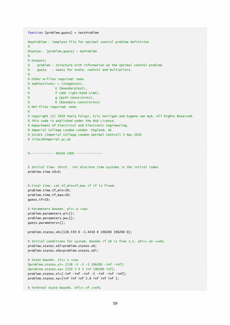
59
function [problem,guess] = testProblem
%myProblem - Template file for optimal control problem definition
%
%Syntax: [problem,guess] = myProblem
%
% Outputs:
% problem - Structure with information on the optimal control problem
% guess - Guess for state, control and multipliers.
%
% Other m-files required: none
% Subfunctions: L (stageCost),
% E (boundaryCost),
% f (ODE right-hand side),
% g (path constraints),
% b (boundary constraints)
% MAT-files required: none
%
% Copyright (C) 2010 Paola Falugi, Eric Kerrigan and Eugene van Wyk. All Rights Reserved.
% This code is published under the BSD License.
% Department of Electrical and Electronic Engineering,
% Imperial College London London England, UK
% ICLOCS (Imperial College London Optimal Control) 5 May 2010
%------------- BEGIN CODE --------------
% Initial time. t0<tf. For discrete time systems is the initial index
problem.time.t0=0;
% Final time. Let tf_min=tf_max if tf is fixed.
problem.time.tf_min=30;
problem.time.tf_max=30;
guess.tf=10;
% Parameters bounds. pl=< p <=pu
problem.parameters.pl=[];
problem.parameters.pu=[];
guess.parameters=[];
problem.states.x0=[138.559 0 -1.4410 0 196200 196200 0];
% Initial conditions for system. Bounds if x0 is free s.t. x0l=< x0 <=x0u
problem.states.x0l=problem.states.x0;
problem.states.x0u=problem.states.x0l;
% State bounds. xl=< x <=xu
%problem.states.xl= [138 -5 -3 -3 196200 -inf -inf];
%problem.states.xu= [150 5 4 3 inf 196200 inf];
problem.states.xl=[-inf -inf -inf -3 -inf -inf -inf];
problem.states.xu=[inf inf inf 2.8 inf inf inf ];
% Terminal state bounds. xfl=< xf <=xfu
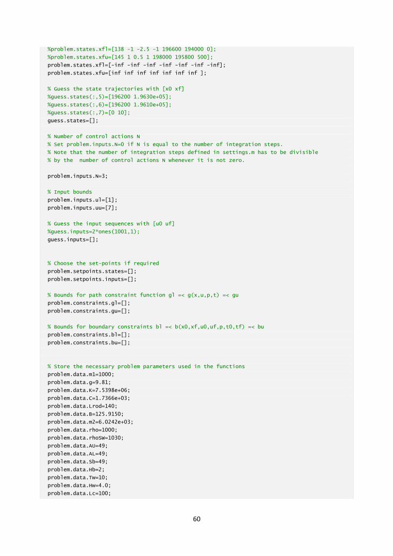
60
%problem.states.xfl=[138 -1 -2.5 -1 196600 194000 0];
%problem.states.xfu=[145 1 0.5 1 198000 195800 500];
problem.states.xfl=[-inf -inf -inf -inf -inf -inf -inf];
problem.states.xfu=[inf inf inf inf inf inf inf ];
% Guess the state trajectories with [x0 xf]
%guess.states(:,5)=[196200 1.9630e+05];
%guess.states(:,6)=[196200 1.9610e+05];
%guess.states(:,7)=[0 10];
guess.states=[];
% Number of control actions N
% Set problem.inputs.N=0 if N is equal to the number of integration steps.
% Note that the number of integration steps defined in settings.m has to be divisible
% by the number of control actions N whenever it is not zero.
problem.inputs.N=3;
% Input bounds
problem.inputs.ul=[1];
problem.inputs.uu=[7];
% Guess the input sequences with [u0 uf]
%guess.inputs=2*ones(1001,1);
guess.inputs=[];
% Choose the set-points if required
problem.setpoints.states=[];
problem.setpoints.inputs=[];
% Bounds for path constraint function gl =< g(x,u,p,t) =< gu
problem.constraints.gl=[];
problem.constraints.gu=[];
% Bounds for boundary constraints bl =< b(x0,xf,u0,uf,p,t0,tf) =< bu
problem.constraints.bl=[];
problem.constraints.bu=[];
% Store the necessary problem parameters used in the functions
problem.data.m1=1000;
problem.data.g=9.81;
problem.data.K=7.5398e+06;
problem.data.C=1.7366e+03;
problem.data.Lrod=140;
problem.data.B=125.9150;
problem.data.m2=6.0242e+03;
problem.data.rho=1000;
problem.data.rhoSW=1030;
problem.data.AU=49;
problem.data.AL=49;
problem.data.Sb=49;
problem.data.Hb=2;
problem.data.Tw=10;
problem.data.Hw=4.0;
problem.data.Lc=100;

61
% Get function handles and return to Main.m
problem.functions={@L,@E,@f,@g,@b};
%------------- END OF CODE --------------
function stageCost=L(x,xr,u,ur,p,t,data)
% L - Returns the stage cost.
% The function must be vectorised and
% xi, ui are column vectors taken as x(:,i) and u(:,i) (i denotes the i-th
% variable)
%
% Syntax: stageCost = L(x,xr,u,ur,p,t,data)
%
% Inputs:
% x - state vector
% xr - state reference
% u - input
% ur - input reference
% p - parameter
% t - time
% data- structured variable containing the values of additional data used inside
% the function
%
% Output:
% stageCost - Scalar or vectorised stage cost
%
% Remark: If the stagecost does not depend on variables it is necessary to multiply
% the assigned value by t in order to have right vector dimesion when called for the
optimisation.
% Example: stageCost = 0*t;
%------------- BEGIN CODE --------------
Hw=data.Hw;
Tw=data.Tw;
Lrod= data.Lrod;
m2=data.m2;
rho=data.rho;
g=data.g;
Lc=data.Lc;
%Defino la ola
xw = Hw/2*sin((2*pi/Tw)*t-(pi/2))+Lrod;
%Define states and setpoints
x1=x(:,1);
x2=x(:,2);
x3=x(:,3);
x4=x(:,4);
x5=x(:,5);
x6=x(:,6);
x7=x(:,7);
62
%Define inputs
u1 = u(:,1);
stageCost = max(abs(x1-xw))*ones(size(x1))-((max(x6)-196200)/rho*g)*AU;
%------------- END OF CODE --------------
function boundaryCost=E(x0,xf,u0,uf,p,tf,data)
% E - Returns the boundary value cost
%
% Syntax: boundaryCost=E(x0,xf,u0,uf,p,tf,data)
%
% Inputs:
% x0 - state at t=0
% xf - state at t=tf
% u0 - input at t=0
% uf - input at t=tf
% p - parameter
% tf - final time
% data- structured variable containing the values of additional data used inside
% the function
%
% Output:
% boundaryCost - Scalar boundary cost
%
%------------- BEGIN CODE --------------
boundaryCost=0;
%------------- END OF CODE --------------
function dx = f(x,u,p,t,data)
% f - Returns the ODE right hand side where x'= f(x,u,p,t)
% The function must be vectorised and
% xi, ui, pi are column vectors taken as x(:,i), u(:,i) and p(:,i). Each
% state corresponds to one column of dx.
%
%
% Syntax: dx = f(x,u,p,t,data)
%
% Inputs:
% x - state vector
% u - input
% p - parameter
% t - time
% data-structured variable containing the values of additional data used inside
% the function
%
% Output:
% dx - time derivative of x
%

63
% Remark: If the i-th ODE right hand side does not depend on variables it is necessary to
multiply
% the assigned value by a vector of ones with the same length of t in order
% to have a vector with the right dimesion when called for the optimisation.
% Example: dx(:,i)= 0*ones(size(t,1));
%
%------------- BEGIN CODE --------------
%Parameters for the definition of the wave and the buoyancy force
Hw=data.Hw;
Tw=data.Tw;
Lrod=data.Lrod;
rhoSW=data.rhoSW;
g=data.g;
Sb=data.Sb;
Hb=data.Hb;
rho=data.rho;
%Define states
x1=x(:,1);
x2=x(:,2);
x3=x(:,3);
x4=x(:,4);
x5=x(:,5);
x6=x(:,6);
x7=x(:,7);
%Definition of the wave
xw = Hw/2*sin((2*pi/Tw)*t-(pi/2))+Lrod;
%Define inputs
u1 = u(:,1);
%Buoyancy force
Fw=(xw-x1+Hb/2)*Sb*rhoSW*g;
%Parameters for ODE equations
K=data.K;
C=data.C;
m1=data.m1;
m2=data.m2;
B=data.B;
AU=data.AU;
AL=data.AL;
%Definition of ODE equations (switching system)
dx(:,1) = x2;
dx(:,2) = -(K/m1)*x1-(C/m1)*x2+(K/m1)*x3+(C/m1)*x4+(Fw/m1)+(K*Lrod/m1)-g;
dx(:,3) = x4;
mup = zeros(size(x4));
index = find(x4<=0.0);
index2 = find(x4>0.0);

64
mup(index) = m2 + rho*0.06*floor(u1(index)).*((x5(index)/rho/g)+100);
dx(index,4) = (K./mup(index)).*x1(index)+(C./mup(index)).*x2(index)-
(K./mup(index)).*x3(index)-((B+C)./mup(index)).*x4(index)-
0.06*(1./mup(index)).*floor(u1(index)).*x5(index)+0.06*(1./mup(index)).*floor(u1(index)).*x6(
index)-g-K*Lrod./mup(index);
dx(index,5) = (rho*g/AU)*0.06*floor(u1(index)).*x4(index);
dx(index,6) = -(rho*g/AL)*0.06*floor(u1(index)).*x4(index);
dx(index2,4) = (K/m2)*x1(index2)+(C/m2)*x2(index2)-(K/m2)*x3(index2)-((B+C)/m2)*x4(index2)-g-
K*Lrod/m2;
dx(index2,5) = 0;
dx(index2,6) = 0;
dx(:,7) = ones(size(x4));
%------------- END OF CODE --------------
function c=g(x,u,p,t,data)
% g - Returns the path constraint function where gl =< g(x,u,p,t) =< gu
% The function must be vectorised and
% xi, ui, pi are column vectors taken as x(:,i), u(:,i) and p(:,i). Each
% constraint corresponds to one column of c
%
% Syntax: c=g(x,u,p,t,data)
%
% Inputs:
% x - state vector
% u - input
% p - parameter
% t - time
% data- structured variable containing the values of additional data used inside
% the function
%
% Output:
% c - constraint function
%
%------------- BEGIN CODE --------------
c=[];
%------------- END OF CODE --------------
function bc=b(x0,xf,u0,uf,p,tf,data)
% b - Returns a column vector containing the evaluation of the boundary constraints: bl =<
bf(x0,xf,u0,uf,p,t0,tf) =< bu
%
% Syntax: bc=b(x0,xf,u0,uf,p,tf,data)
%
% Inputs:
% x0 - state at t=0
% xf - state at t=tf
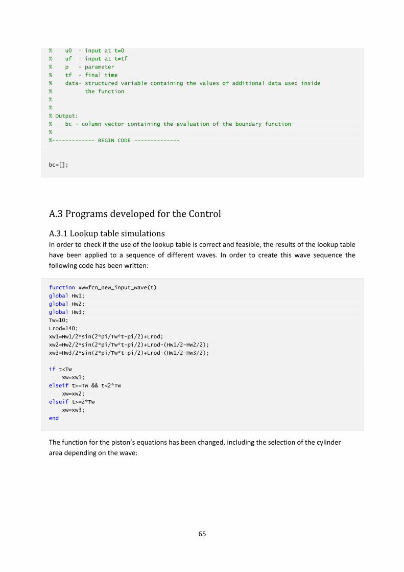
65
% u0 - input at t=0
% uf - input at t=tf
% p - parameter
% tf - final time
% data- structured variable containing the values of additional data used inside
% the function
%
%
% Output:
% bc - column vector containing the evaluation of the boundary function
%
%------------- BEGIN CODE --------------
bc=[];
A.3 Programs developed for the Control
A.3.1 Lookup table simulations In order to check if the use of the lookup table is correct and feasible, the results of the lookup table
have been applied to a sequence of different waves. In order to create this wave sequence the
following code has been written:
function xw=fcn_new_input_wave(t)
global Hw1;
global Hw2;
global Hw3;
Tw=10;
Lrod=140;
xw1=Hw1/2*sin(2*pi/Tw*t-pi/2)+Lrod;
xw2=Hw2/2*sin(2*pi/Tw*t-pi/2)+Lrod-(Hw1/2-Hw2/2);
xw3=Hw3/2*sin(2*pi/Tw*t-pi/2)+Lrod-(Hw1/2-Hw3/2);
if t<Tw
xw=xw1;
elseif t>=Tw && t<2*Tw
xw=xw2;
elseif t>=2*Tw
xw=xw3;
end
The function for the piston’s equations has been changed, including the selection of the cylinder
area depending on the wave:

66
function ret=fcn_piston_acc_for_model2_PruebaD(x1,x2,v1,v2,p1,p4,t)
% Definition of parameters
global K
global mp
global Lc
global C
global B
global Ac1;
global Ac2;
global Ac3;
rho = 1000; % Water density (Kg/m^3)
rhoSt = 7850; % Steel density (Kg/m^3)
global g;
% Rod-piston-cylinder
Rrod = 0.04; % Rod radius (m)
Lrod = 140; % Rod length (m)
mrod = rhoSt*pi*Rrod^2*Lrod; % Rod mass (Kg)
Tw=10;
m2 = mp+mrod;
%Look up table
if t<Tw
Aclook=Ac1;
elseif t>=Tw && t<2*Tw
Aclook=Ac2;
elseif t>=2*Tw
Aclook=Ac3;
end
if v2>=0
mup = m2+rho*Aclook*((p1/rho/g)+Lc);
ret = (K/mup)*x1+(C/mup)*v1-(K/mup)*x2-((B+C)/mup)*v2-(Aclook/mup)*p1+(Aclook/mup)*p4-g-
K*Lrod/mup;
elseif v2<0
mdown = m2;
ret = (K/mdown)*x1+(C/mdown)*v1-(K/mdown)*x2-((B+C)/mdown)*v2-g-K*Lrod/mdown;
end
And the same was done for the equation of the flow rate:
Function Q=fcn_flow(v2,t)
global Ac1;
global Ac2;
global Ac3;
Tw=10;
if t<Tw
Aclook=Ac1;
elseif t>=Tw && t<2*Tw
Aclook=Ac2;
elseif t>=2*Tw
Aclook=Ac3;
end

67
if v2>=0
Q = Aclook*v2;
else
Q = 0;
end
end
A.3.2 Exhaustive search The code of the ‘Running all combinations’ program mentioned in the section 4.4.5 is shown below:
global Ac1
global Ac2
global Ac3
Parameters_and_Variables;
%Generating all the combinations between the available areas of the
%cylinder
AreasCyl=[0.06,0.18,0.30];
AreasComb=npermutek(AreasCyl,NumberWaves);
%Vector of Cost function J for each combination of areas
sizeaux=size(AreasComb);
sizeJ=sizeaux(1);
Jvector=ones(sizeJ,1);
%Simulate the model for each combination of areas
i=1;
while i<=sizeJ
Ac1=AreasComb(i,1);
Ac2=AreasComb(i,2);
Ac3=AreasComb(i,3);
SimOut=sim('Prueba_Simulink_Experimento_control_2');
CostValue=20*max(abs(x1-xw))-((max(p1)-p10)/(rho*g))*AU;
Jvector(i)=CostValue;
i=i+1;
end
OptimalCost=min(Jvector)
auxpos=find(Jvector<=OptimalCost);
OptimalAreas=AreasComb(auxpos,:)
As seen in the program, we used a function called 'npermutek', which generates all possible
combinations between the available areas of cylinder for the number of waves that will be
introduced to the system.
A.3.3 Implementation of the MPC For calculating the optimal input for a sequence of 6 waves the following code has been used:
global Ac1
global Ac2
global Ac3
global Ac4
global Ac5
global Ac6
Parameters_and_Variables;
%Generating all the combinations between the available areas of the

68
%cylinder
AreasCyl=[0.06,0.18,0.30];
AreasComb=npermutek(AreasCyl,NumberWaves);
%Vector of Cost function J for each combination of areas
sizeaux=size(AreasComb);
sizeJ=sizeaux(1);
Jvector=ones(sizeJ,1);
%Simulate the model for each combination of areas
i=1;
while i<=sizeJ
Ac1=AreasComb(i,1);
Ac2=AreasComb(i,2);
Ac3=AreasComb(i,3);
Ac4=AreasComb(i,4);
Ac5=AreasComb(i,5);
Ac6=AreasComb(i,6);
SimOut=sim('Dynamical_Single_Piston_Pump_model');
CostValue=20*max(abs(x1-xw))-((max(p1)-p10)/(rho*g))*AU;
Jvector(i)=CostValue;
i=i+1;
end
OptimalCost=min(Jvector)
auxpos=find(Jvector<=OptimalCost);
OptimalAreas=AreasComb(auxpos,:)
The program that has been used to implement the MPC controller has the following code:
global Hworiginal
global Hw1aux
global Hw2aux
global Hw3aux
global Abuena
global Hw1;
global p1ini;
global p4ini;
global tf;
%Implementation of the MPC controller
t0=0;
WindowWidthMPC=3;
Parameters_and_Variables;
Hworiginal=Hw1;
simtimeaux = WindowWidthMPC*Tw;
%First initial conditions
x1ini=Lrod+0.5*Hb-((m1+mp+mrod+rho*Ac*(Lc+HU0))/(Sb*rhoSW))-Hw1/2;
v1ini=0;
x2ini=+0.5*Hb-((m1+mp+mrod+rho*Ac*(Lc+HU0))/(Sb*rhoSW))-Hw1/2;
v2ini=0;
p1ini=p10;
p4ini=p40;
%Creation of the vectors for the state space variables
tpropio=ones((simtime/timestep)+1,1);
xwdef=ones((simtime/timestep)+1,1);
x1def=ones((simtime/timestep)+1,1);
v1def=ones((simtime/timestep)+1,1);
x2def=ones((simtime/timestep)+1,1);

69
v2def=ones((simtime/timestep)+1,1);
p1def=ones((simtime/timestep)+1,1);
p4def=ones((simtime/timestep)+1,1);
Qdef=ones((simtime/timestep)+1,1);
Fbuoydef=ones((simtime/timestep)+1,1);
AreasUsed=ones(1,NumberWaves2sim);
tf=10;
j=1;
k=1;
while tf<=simtime
tf
Hw1aux=Heights(j);
Hw2aux=Heights(j+1);
Hw3aux=Heights(j+2);
Running_all_combinations;
Abuena=OptimalAreas(1);
AreasUsed(j)=Abuena;
%Implementation of the Optimar area found by the MPC controller, and
%simulation of the system for the next wave.
SimOut=sim('Dynamical_Model_SPP');
%Update of the initial conditions for the models (current conditions)
x1ini=x1(end);
v1ini=v1(end);
x2ini=x2(end);
v2ini=v2(end);
p1ini=p1(end);
p4ini=p4(end);
%The results of the simulations are added to the solution vectors
tpropio(k:((tf/timestep)+1))=t;
xwdef(k:((tf/timestep)+1))=xw;
x1def(k:((tf/timestep)+1))=x1;
v1def(k:((tf/timestep)+1))=v1;
x2def(k:((tf/timestep)+1))=x2;
v2def(k:((tf/timestep)+1))=v2;
p1def(k:((tf/timestep)+1))=p1;
p4def(k:((tf/timestep)+1))=p4;
Qdef(k:((tf/timestep)+1))=Q;
Fbuoydef(k:((tf/timestep)+1))=Fbuoy;
%
t0=tf;
tf=tf+Tw;
j=j+1;
k=k+(Tw/timestep);
end
AreasUsed
Plots
Explanation of the changes made in the 2 models (Model A and Model B) Model A The model A is practically equal to the model used in 'description of the dynamic model' (section 2.2). We just implemented the 6 waves input, and established the updated initial conditions in each case.

70
Model B To develop the model B we started from the model used in the section 4.4.1, in which all possible combinations of piston areas were tested for the input waves and the optimal combination was found. The most important change in the development of this model has been to ensure that the model
always uses the correct initial conditions. These initial conditions are found in model A, which
represents the actual WEC.

71
A.4 Different responses changing different parameters
Par
ame
ter/
Var
iab
leV
alu
eV
pum
ped
(m3 )
Max
imu
m o
f p
isto
n's
ve
loci
ty (
m/s
)(m
)(m
)T w
orst
(K
N)
Are
a o
f cy
lin
de
r (m
2 )0,
120,
4917
1,90
640,
9308
5,17
5450
8,56
95
0,21
0,74
452,
1042
0,96
684,
6228
741,
6429
0,27
0,98
862,
2435
0,95
724,
5385
907,
8828
0,35
1,25
642,
3656
0,97
364,
3947
1124
,100
0
0,5
1,43
822,
4722
0,99
744,
2324
1525
,000
0
Bu
oy'
s m
ass
(kg)
1000
0,49
171,
9064
0,93
085,
1754
508,
5695
500
0,49
131,
9121
0,94
045,
2362
503,
518
2000
0,49
091,
9146
0,91
545,
0579
523,
7064
1000
00,
5042
1,79
220,
7816
3,94
4960
8,79
54
K (
spri
ng
con
stan
t, N
/m)
7,53
98E+
060,
4917
1,90
640,
9308
5,17
5450
8,56
95
1,50
80E+
070,
4906
1,91
060,
9343
5,17
4451
0,59
48
3,76
99E+
060,
4928
1,89
920,
9257
5,19
0450
8,20
09
1,50
80E+
080,
4889
1,89
470,
937
5,16
3850
8,56
62
7,53
98E+
050,
4554
2,07
340,
9436
5,11
5751
1,86
16
Pis
ton
's m
ass
(kg)
500
0,49
171,
9064
0,93
085,
1754
508,
5695
1000
0,49
191,
906
0,92
315,
1178
520,
9737
100
0,49
141,
9166
0,93
855,
224
501,
5727
Ro
d m
ate
rial
Ste
el
0,49
171,
9064
0,93
085,
1754
508,
5695
Cu
pro
nic
kel (
de
nsi
ty =
890
0
kg/m
^3, Y
ou
ng
mo
du
lus
=
135G
Pa)
0,49
071,
9131
0,91
775,
0958
527,
4502
Cyl
ind
er
len
gth
(m
)10
00,
4917
1,90
640,
9308
5,17
5450
8,56
95
200
0,45
812,
1421
0,96
24,
579
803,
6450
500
0,37
072,
4701
0,99
64,
3772
1652
,800
0
250,
5023
1,82
890,
9214
5,69
8833
3,53
61
Are
a u
pp
er
and
low
er
rese
rvo
ir (
m)
490,
4917
1,90
640,
9308
5,17
5450
8,56
95
100
0,49
171,
9078
0,93
15,
1753
507,
6989
200
0,49
21,
9099
0,93
085,
1759
508,
2751
Dam
pin
g co
eff
icie
nt
(N·s
/m)
1736
,600
00,
4917
1,90
640,
9308
5,17
5450
8,56
95
1736
6,00
000,
4918
1,90
470,
9316
5,17
6950
9,47
20
173,
6600
0,49
191,
9059
0,93
115,
1796
509,
5606
B c
oe
ffic
ien
t (N
·s/m
)12
5,91
500,
4917
1,90
640,
9308
5,17
5450
8,56
95
500,
0000
0,49
121,
8951
0,93
185,
1751
509,
6012
2000
,000
00,
4888
1,86
050,
9339
5,17
6351
1,76
65
72
Bibliography
[1] National Research Council. America's Climate Choices: Panel on Advancing the Science of Climate
Change. Washington, D.C. : The National Academies Press, 2010.
[2] Tiwari, G. and Mishra, R. Advanced renewable energy sources. Cambridge : RSC Publishing, 2012.
[3] Observ'ER. The state of renewable energies in europe. Paris : EuroObserv'ER Report, 2013.
[4] Vakis, Antonis. Tribological model of a single-piston pump for a novel wave energy converter.
Groningen : University of Groningen, 2013.
[5] Meijer, Harmen. Research Design: Simulating a piston-type hydraulic pump fot the Ocean Grazer.
MSc Thesis. Groningen : University of Groningen, 2014.
[6] Prins, Wout A. Method and system for extracting kinetic energy from surface waves of a water.
2013. P101922PC00.
[7] Vakis, Antonis I., Prins, Wout A. and Meijer, Harmen. First steps in the design and construction
of the Ocean Grazer. 2014.
[8] Martí Saumell, Josep. Dynamical modelling, analysis and control design of a distributed sea wave
energy storage system MSc Thesis. 2013.
[9] Liberzon, Daniel. Switching in systems and control. University of Illinois : Springer, 2003.
[10] Abraham, E. and Kerrigan, E.C. Optimal Active control and Optimization of a Wave Energy
Converter. Sustainable Energy. IEEE Transactions on 4, 2013. 324-332.
[11] Lane, David M. Introduction to Statistics. Texas : University of Rice, 2013.
[12] Departamento de Matemáticas. Análisis de datos. Madrid : Universidad Autónoma de Madrid,
2011.
[13] Astrom, K. and Hagglund, T. PID controllers: Theory, Design, and Tuning. ISA, 1995.
[14] Qin, S.Joe and Badgwell, Thomas. A survey of industrial model predictive control technology
Report. Texas : University of Texas, 2002.
[15] Di Ruscio, David. Model Predictive Control and optimization Lecture Notes. Telemark University
College, 2001.
[16] Ram, Babu. Numerical Methods. Pearson Education India, 2010.
[17] Falugi, Paola, Kerrigan, Eric and van Wyk, Eugene. Imperial College London Optimal Control
Software User Guide (ICLOCS). London. 2010.
[18] Kawajir, Yoshiaki, Vigerske, Stefan and Wachter, Andreas. Introduction to IPOPT. 2013.

73
[19] Welink, J. Creating a scale model deisgn for the Ocean Grazer project, Bachelor thesis.
University of Groningen, 2014.
[20] Drtina, P. and Sallaberger, M. Hydraulic turbines - basic principles and state-of-the-art
computational fluid dynamics applications. Zürich. 1999.
[21] Calvert, J.B. [Online] 11 February 2010.
https://mysite.du.edu/~jcalvert/tech/fluids/turbine.htm.
[22] Seborg, Dale E., Edgar, Thomas F. and Mellichamp , Duncan A. Process Dynamics and Control.
John Wiley & Sons, 2010.
[23] Allgower, Frank, Findeisen, Rolf and Zoltan , K. Nagy. Nonlinear Model Predictive Control: From
Theory to Application. Birkhauser, 2000. 3034895542.
[24] Alexey, F. Izmailov and Mikhail, V. Solodov. Newton-Type Methods for Optimizations and
Variational Problems. Springer, 2014. 3319042467.