University of Hamburg
Faculty of Economics Chair of International Relations
Prof. Dr. Thomas Straubhaar
Diploma Thesis:
Multinational Enterprises and
Exchange Rates
04th of October 2007
By: Signe Nelgen

I I
Table of Contents
LIST OF ABBREVIATIONS III
LIST OF TABLES IV
LIST OF FIGURES IV
1 INTRODUCTION 1
2 THEORETICAL BACKGROUND 5
2.1 THE GRAVITY MODEL........................................................................................................................... 5 2.2 DEFINITIONS OF FIXED EXCHANGE RATE REGIMES .............................................................................. 8 2.3 CLASSIFYING EXCHANGE RATE REGIMES............................................................................................. 8 2.4 INDIRECT PEGGED EXCHANGE RATE REGIMES................................................................................... 13 2.5 DE FACTO VS. DE JURE....................................................................................................................... 14 2.6 EXCHANGE RATE REGIMES IN DEVELOPING COUNTRIES.................................................................... 17 2.7 LIMITATIONS OF THE DE FACTO CLASSIFICATION............................................................................... 18
3 THEORETICAL AND EMPIRICAL LITERATURE ON FDI AND EXCHANGE RATES 20
3.1 FDI AND (CURRENT, EXPECTED) REAL BILATERAL EXCHANGE RATES.............................................. 20 3.2 FDI AND EXCHANGE RATE VOLATILITY ............................................................................................. 22 3.3 FDI AND EXCHANGE RATE REGIMES.................................................................................................. 28 3.4 SUMMERY OF THE LITERATURE ON FDI AND EXCHANGE RATE VARIABLES....................................... 29
4 EMPIRICAL ANALYSIS: EXCHANGE RATE REGIMES AND FDI 31
4.1 METHODOLOGY, CONTROL VARIABLES AND SAMPLE ........................................................................ 31 4.2 FDI VARIABLES .................................................................................................................................. 34 4.3 EXCHANGE RATE VARIABLES ............................................................................................................. 36 4.4 EMPIRICAL RESULTS............................................................................................................................ 38
5 CONCLUDING REMARKS AND POLICY IMPLICATIONS 48
REFERENCES 50
APPENDIX A: DEFINITION OF VARIABLES AND DATA SOURCES 56
APPENDIX B: SOURCE COUNTRY SAMPLE 57
APPENDIX C: HOST COUNTRY SAMPLE 57
III
List of Abbreviations..................................................................
CPI Consumer Price Index
ECU European Currency Unit
EMU European Monetary Union
FDI Foreign Direct Investment
GARCH Generalised Autoregressive Conditional Heteroscedasticity
IMF International Monetary Fund
GDP Gross Domestic Product
GNP Gross National Product
MNE Multinational Enterprise
OLI Ownership, Location, Internalisation
OLS Ordinary Least Squares
PPP Purchasing Power Parity
RTA Regional Trade Agreement
SDR Special Drawing Right
UNCTAD United Nations Conference on Trade and Development
IV
List of Tables
Table 1: Distribution of FDI by Region, 1980-2005 (percent), Source: UNCTAD (2006).......2 Table 2: Evolution of exchange rate regimes: Reinhart and Rogoff natural classification (percentage of members in each category), Source: Eichengreen and Razo-Garcia (2006)...38 Table 3: Fixed Effects Estimation: Dependent Variables FDI 1 and FDI 2............................39 Table 4: Fixed Effects Estimation: Dependent Variables FDI 3 - FDI 8.................................43 Table 5: Fixed Effects Estimation: Dependent Variables FDI 1 and FDI 2............................46 Table 6: Fixed Effects Estimation: Dependent Variables FDI 3 – FDI 8................................47
List of Figures
Figure 1: Development of FDI Inflows, Global and by Group of Economies, 1980-2005 (Billions of US Dollars), Source: UNCTAD (2006)...................................................................1 Figure 2: Total Net Resource Flows to Developing Countries, by Type of Flow, 1990-2005 (Billions of US Dollars), Source: UNCTAD (2006)...................................................................2 Figure 3: Comparison of Exchange Rate Arrangements According to the IMF Official and.15 Figure 4: Trend toward Polarization of Exchange Rate Regimes across Country Groups in 1990 and 2001 (in percent of membership in each group), Source: Bubula and Ötker-Robe (2002).......................................................................................................................................18

1
1 Introduction
A multinational enterprise (MNE) is a firm that is engaged in production facilities in at least
two countries. In this way, it establishes lasting interests in foreign markets. These long-term
activities of MNEs are called foreign direct investment (FDI).
Over the last 20 years, MNEs have become increasingly important players in the world
economy (Figure 1). While world FDI inflows averaged US$ 100 billion during the 1980s,
there were periods with rapid increases during the late 1980s and 1990s. At the end of the last
century, during the height of the “dot com bubble”, FDI inflows reached a peak at US$ 1,400
billion annually. With the sudden end of this boom, and investors’ flagging confidence, FDI
flows collapsed to about US$ 400 billion annually in 2003 and only started to recover
recently, spurred by solid growth prospects in the world economy, particularly in countries
like China, India and those of the former Eastern bloc. In 2005, world FDI inflows reached
US$ 916 billion. Taking a long term view, it is evident that FDI has grown by an order of
magnitude in the last two decades.
Figure 1: Development of FDI Inflows, Global and by Group of Economies, 1980-2005
(Billions of US Dollars), Source: UNCTAD (2006).
Because the surge in FDI flows has happened relatively recently, reliable data and
economic studies on its determinants and effects are only now becoming available and
possible. At the same time, the sheer magnitude of FDI flows and their effects on economic,
social, and environmental development has resulted in a heightened interest in studies on FDI.

2
Most of the rapid increase in FDI is attributed to activities in developed countries. FDI
flows into developing countries were, and still are only a fraction of those into developed
countries. During the period 1978 to 1980, developed and developing countries received
about 80 and 20 percent of world FDI inflows, respectively, whereas 97 and 3 percent of FDI
outflows originated from developed and developing countries respectively (Table 1). In the
last period for which official data are available, the years from 2003 to 2005, developing
countries had almost doubled their share of total FDI inflows to 36 percent and quadrupled
their share of total FDI outflows to 12 percent. FDI flows into developing countries have also
been considerably more stable than those into developed countries (Figure 1).
Region
1978-1980 1988-1990 1998-2000 2003-2005 1978-1980 1988-1990 1998-2000 2003-2005
Developed Economies 79.7 82.5 77.3 59.4 97.0 93.1 90.4 85.8
Developing Economies 20.3 17.5 21.7 35.9 3.0 6.9 9.4 12.3
South-East Europe and CIS 0.02 0.02 0.9 4.7 .. 0.01 0.2 1.8
World 100.0 100.0 100.0 100.0 100.0 100.0 100.0 100.0
Inf low Outf low
Table 1: Distribution of FDI by Region, 1980-2005 (percent), Source: UNCTAD (2006).
Both policy-makers and economists consider FDI flows as a valuable support of
domestic economic growth. This has various reasons: As shown in Figure 2 below, FDI
inflows are the largest component of net resource flows into developing countries.
Figure 2: Total Net Resource Flows to Developing Countries, by Type of Flow, 1990-2005
(Billions of US Dollars), Source: UNCTAD (2006).
At the same time, they are more stable than other (portfolio) investment flows, and
appear to be relatively dependable even in times of political and currency crises (Lipsey

3
2001). This is the case because the foreign subsidiaries were able to finance investments
internally, through their parent companies, which are usually based in countries with
economic stability.
Moreover, FDI flows into developing countries lead to a transfer of technical and
managerial know-how which would otherwise be out of their reach, since their own domestic
enterprises are generally relatively small, undercapitalised and technologically backwards.
The know-how brought into their foreign subsidiaries by MNEs is spread to other
local companies by staff fluctuation and by doing business with local suppliers. In many
cases, MNEs encourage and promote their subsidiaries’ efforts to gain access to foreign
markets and to earn foreign currencies and thereby improve the host countries balance of
payments position. Most importantly, by establishing productions in developing countries,
MNEs generate revenues, which in turn are partially paid out locally to the factors of
production and as taxes. This, of course, provides a boost to local economic growth. These
facts explain why FDI is considered to be so important, in particular for developing countries,
and why countries compete for it (Esaka 2007).
There are two main ways to look at FDI flows, initiated by MNEs. One can investigate
their determinants or analyse their effects on economic development. This study focuses on
the determinants of FDI flows. Such determinants are, for example, the size and development
of the host country’s market, its endowment with local factors of production, its tax system,
political stability, and its infrastructure.1
One determinant of FDI that has as yet received little attention is the influence of the
exchange rate regime chosen by a host country. Macroeconomic stability of a host country is
an important factor influencing a MNE’s decision to engage in FDI. Therefore, one could also
expect the stability and the credibility introduced by fixed exchange rate regimes or currency
pegs to have a significant influence on FDI. A fixed exchange rate regime is expected to
enhance a country’s international credibility and to reduce exchange rate volatility by linking
the currency to a “trusted” anchor currency. This imported credibility and stability could
possibly encourage FDI inflows. Therefore, it would be interesting to investigate whether this
effect actually exists.
However, this is obstructed by the difficulty in observing the “actual” exchange rate
regime. This problem arises because there may be a discrepancy between the exchange rate
regime a country officially announces (i.e., its de jure exchange rate regime) and the exchange
1 For in-depth analysis, see Bloningen (2005) and Chakrabarti (2001).

4
rate regime it actually practises (i.e., its de facto exchange rate regime). Evidently, the
compilation of the actual, de facto exchange rate classification is fraught with problems.
Countries try to hide their real intentions and one has to rely on surrogate measures as
indicators for the unobservable, actual exchange rate regime, prevailing at a given time. There
are, of course, many ways to extract the underlying de facto exchange rate regime. The
different approaches to this problem will be discussed in detail in chapter 2.
In the context of this study, the question of which exchange rate regime classification
best characterises the actual exchange rate regime is of minor importance. Instead, the
exchange rate classification that is “used” by MNEs is of interest. Although the de facto
exchange rate regimes should be more important for MNEs’ decisions, it is nevertheless
possible that they rely on the de jure exchange rate regimes because of lack of better
information. However, MNEs usually have good commercial contacts to the countries they
plan to invest in. Also, major investments are based on thorough preparations. It is therefore
unrealistic to assume that they do not know of parallel markets, hidden exchange rate
manipulations and other ways to bypass the official, de jure exchange rate regimes. Therefore,
it can be assumed that MNEs engaging in FDI will be generally well informed and base their
decisions on the de facto exchange rate regimes, whose effects they will have observed in the
time preceding the investment. This study uses a de facto exchange rate classification as an
explanatory variable of FDI for a large country sample.
As mentioned above, exchange rate regimes may be an important factor in the decision
to invest in a certain country. Chapter 2 describes different exchange rate regimes and
methods of classification. The de jure and de facto classification systems are presented, and
their particular advantages and disadvantages are laid out. Likewise, the impact of exchange
rate regimes on developing countries and the way these countries handle exchange rate
regimes are discussed.
Chapter 3 surveys the theoretical and empirical literature on the exchange rate as a
determinant of FDI flows. This chapter gives an overview on the studies dealing with the
influence of the exchange rate level, the exchange rate volatility and the exchange rate regime
on FDI flows. These studies used different methods and different country samples. As a
consequence, they obtained different results.
There are only a few papers analysing the link between FDI and exchange rate
regimes. In particular, data for a large sample of developing countries have only become
available recently. Chapter 4 tries to capture and quantify the influence of fixed exchange rate
5
regimes on FDI flows. This study focuses on the effect of a fixed exchange rate regime,
imposed at a bilateral level, using bilateral FDI data for flows from one source country to
another host country. Panel data covering the time span from 1978 to 2004 for 110 host and
31 source countries are used. Concerning the de facto exchange rate regimes there were only
data signalling that “a” specific form of exchange rate regime existed for a certain host
country, without specifying the anchor currency. In effect, this meant that there were no data
at a bilateral level for those cases with a fixed or pegged currency regime. Therefore, existing
exchange rate regime classifications are extended by extracting the bilateral information from
published International Monetary Fund (IMF) and World Bank exchange rate records.
The effects of different FDI determinants are quantified by using a gravity-type model.
This approach, motivated by Carr et al. (2001), has been applied by many authors for
analysing bilateral FDI. Most of these studies concentrated on data for developed countries
and on relatively short periods. This study tries to overcome this selection bias by using a
large sample, including observations covering a long time span for many developing countries
as host and as source countries.
In contrast to a simple pooled OLS2 analysis, a fixed-effects estimation is selected as
the estimation method. It is plausible to assume that FDI inflows into individual countries
differ, because of time invariant features (e.g., colonial past, languages, etc.), and that these
influences are captured by the “fixed coefficients” (i.e., dummy variables for each country). It
is important to note that the analysis uses new bilateral data on an extended sample to shed
some light on the as yet sparsely researched effects of fixed exchange rate regimes on FDI
flows.
2 Theoretical background
2.1 The Gravity Model
The gravity model was introduced by Tinbergen (1962) into empirical economic analysis. He
derived it from Newton´s gravity equation in physics, which states that the attractive forces
between two objects are proportional to their masses and inversely proportional to the square
of their distance. Tinbergen (1962) used it to investigate international trade flows by
explaining the volume of bilateral trade flows by population size, GDP of home and host
country and distance between host and home country. Later on, the gravity model was
2 Ordinary Least Squares

6
employed to model various other types of flows, such as migration, commuting, tourism,
commodity shipping and also FDI.
A gravity model very similar to that first applied to international trade flows was later
used to describe the determinants of FDI. In general, economic flows from an origin i (source
country) to a destination j (host country) are explained by economic forces at the flow’s
origin, economic forces at the flows’s destination, and economic forces either aiding or
restricting the flow’s movement from origin to destination. Studies of international FDI
analysing bilateral FDI panel data typically use the following form of the gravity equation:
ijtijijjtitjtitijt uATHDISTPOPPOPGDPGDPFDI 654321 )()()()()()(0βββββββ= (1)
where ijtFDI represents the value of the FDI flows from country i to country j at time t.
itGDP and jtGDP , respectively, denote the value of nominal GDP in the home country i and
the host country j , and itPOP and jtPOP the population size of the countries at time t.
ijDIST stands for the distance between the economic centre of the origin country i and the
destination country j . ijATH represents other factors, either aiding or resisting FDI between
i and j at the time t, and ijtu is a log-normally distributed error term with 0)(ln =ijtuE .
Despite the good statistical matches obtained by using this type of model, the
theoretical foundation of the model remained intuitive for a long time. First attempts to
provide theoretical foundations were made by Linnemann (1966), Anderson (1979) and
Bergstrand (1985, 1989). A common result of these studies is that the gravity equation can be
thought of as a reduced form equation incorporating supply and demand factors of two
countries. Carr et al. (2001) proposed gravity variables that account for the market size of the
two countries, for differences in skilled labour abundance between the two countries, the
distance between the two countries and their respective indices for trade and investment costs.
They found the knowledge capital model to be a helpful theoretical basis for the derivation of
the gravity model of FDI flows. The resulting equations are manageable and yield clear-cut
testable hypotheses. Carr et al. (2001) tested the hypotheses derived from the knowledge
based capital model with regard to the importance of multinational activity between countries
as a function of certain characteristics of those countries.
Gast (2005) specified a gravity equation for bilateral FDI flows. He tried to stay close
to the knowledge capital framework, proposed by Carr et al. (2001). In contrast to Carr et al.,
but similar to Bergstrand (1985, 1989), he included exchange rates and price indices into the

7
empirical specification of the gravity equation in order to control for relative price effects.
The specification is as follows:
ititijtijtijtijt EXCHSTOCKSKILLDIFFGDPDIFFGDPSUMFDI $54321 βββββ ++++=
itjtitjtitjt TRAEATYRISKRISKCPICPIEXCH 1110987$6 ββββββ ++++++
ijtijijt
jtitjt uaYDDISTFREEFREETREATY ++++++ *15141312 ββββ (2)
where ijtGDPSUM stands for the sum of both countries’ GDP to control for the total market
size, ijtGDPDIFF is an indicator of relative country size in terms of GDP and ijtSKILLDIFF
represents the endowment differences in skilled labour. Furthermore a stock market indicator
itSTOCK is included and itEXCH$ and jtEXCH$ are the exchange rates of the countries j
and i with the US Dollar. Instead of calculating the real exchange rate explicitly, they
included the consumer price indices of the source and the host country as separate terms,
itCPI and jtCPI . There are further variables to control for the political environment,
transport and investment costs. itRISK and jtRISK are country risk indicators, itTREATY and
jtTREATY stands for the number of bilateral investment treaties each country has signed with
other countries. itFREE and jtFREE are indicators for economic freedom. ijDIST is the great
circle distance between the countries’ capitals. This variable is weighted with year dummies
(YD) to introduce its changing influence on the dependent variable over time.
Most empirical studies focussing on FDI flows refer to the gravity equation of Carr et
al. (2001) as the theoretical foundation. The equation derived by them refers to affiliate sales
but not to FDI flows. There is no doubt that affiliate sales und FDI flows are closely related to
each other. Nevertheless, they are not identical. For example, it is possible for a MNE to raise
the capital for an investment in a foreign country directly in the host country’s capital market,
so that there is no FDI flow (in the strict sense). Therefore, the sales of the subsidiary or
affiliate take place without an FDI being officially registered.
Below a short exposition of the different variants of pegged regimes is given, which
will be elaborated on in the empirical analysis in chapter 4. Basically one can classify pegged
regimes into hard pegs on the one hand and traditional pegs on the other.

8
2.2 Definitions of Fixed Exchange Rate Regimes Hard Pegs: Dollarization, Currency Boards and Monetary Unions
Hard pegs represent the extreme form of fixed exchange rate regimes and include
dollarization, currency boards and monetary unions. Using the regime of dollarization, the
country abandons its own currency completely and establishes a foreign currency as the legal
tender. Nevertheless, it sometimes issues domestic coins and notes, but this is not used as an
independent monetary policy. A currency board implies that the exchange rate is pegged to a
foreign currency by giving the exchange rate regime and the exchange rate parity legal status.
Usually those laws specify the minimum amount of international reserves to be held by the
central bank as percentage of a pre-specified monetary aggregate. Another form of a hard peg
is the monetary union, which means that the countries use one common currency and have
one common central bank and monetary policy (e.g., the European Monetary Union (EMU)).
Traditional Pegs: Currency Unions and Basket Pegs
Traditional pegs constitute single currency unions and basket pegs. If a country chooses a
single currency peg, its exchange rate is pegged to a fixed par-value to the currency of a
single foreign country. The announced par-value is adjustable in case of fundamental
disequilibrium. The credibility of this form of a peg increases with the level of central bank
reserves. Since in general the reserves do not cover all domestic liabilities, there is some
leeway for discretionary monetary policy. Unlike a single currency peg, the basket peg means
that the currency is pegged to a basket of several currencies (Ghosh, Gulde, Wolf, 2002). 3
2.3 Classifying Exchange Rate Regimes
For potential FDI investors, it would be useful to have a variable from which they could
reliably discern the exchange rate regime of a host country. Similarly, for an empirical
analysis one needs a simple variable that represents the different exchange rate regimes as
discrete classes. At first, this seems a simple problem. However, closer inspection reveals that
there are a multitude of intermediate exchange rate regimes, like cooperative regimes,
crawling pegs, target zones and bands, which cannot be differentiated easily. Even the clear-
cut extremes of fixed and floating exchange rate regimes rarely occur in their “pure” form in
practice.
3 A composite currency like the SDR or the previously used ECU is possible as well.

9
Often, there is a discrepancy between the exchange rate regime officially announced
and that effectively conducted, because governments and central banks have many subtle
ways of intervening covertly on currency markets. Consequently, there is no clear-cut and
objectively correct classification. Any assignment of countries to a few idealised types of
exchange rate regimes will be highly subjective and depend to a large degree on personal
judgment. Not surprisingly, there are several categorizations of countries according to the
exchange rate regimes, assigned to them by different researchers (Ghosh, Gulde and Wolf
2002).
The task of categorizing countries according to a type of exchange rate regime is
complicated even further by the fact that countries continuously try to pursue the goals of the
impossible trinity: independent monetary policy, rigidly fixed exchange rates, and complete
capital mobility, by taking actions that influence their exchange rate regime more or less
directly. Also, exchange rate regimes are often changed under great pressure in situations of
crisis under great uncertainty. Therefore, in the aftermath of the crisis the handling of and the
adherence to the officially announced exchange rate regimes are often “corrected” and vary
strongly over time. This again results in frequent, more or less perceptible changes of the
exchange rate regimes (Frankel 1999).
Each IMF member country has to report and publish the stated intentions of their
central bank each year. According to this announcement, the country is “de jure” classified as
belonging to a type of exchange rate regime.4 This classification according to a public policy
statement has to be regarded as an indication for the private sector to guide expectations and
to influence economic activities in a country. As mentioned above, there are many reasons
why countries do not (strictly) adhere to their announcements. Obviously, the official IMF
classification, which relies on these official announcements, deviates from reality in many
cases. Classifying these regimes according to the official announcements of the countries
could be misleading.
Ghosh, Gulde and Wolf (2002) speak about “soft pegs” and “hard floats” if countries
which are not able to restrict their inflation in a way necessary to maintain the fixed exchange
rate parity prop up their currencies using interventions, or if a country may officially
announce a floating regime but nevertheless intervenes in the foreign exchange rate market.
4 These are given in the IMF’s Annual Report on Exchange Rate Arrangements and Exchange Restrictions

10
Other countries abuse their credibility by expansionary policies which are inconsistent with
their stated goals and the long-term sustainability of the peg (Tornell and Velasco 2000).
Hence, economists took great effort to find a realistic classification system that better
describes the “de facto” exchange rate system of the countries. Not surprisingly, economists
developed different ways to classify countries’ exchange rate regimes. Most frequently cited
is the classification of Carmen Reinhart and Kenneth Rogoff, which they call “natural
classification”. It is based on an analysis of the parallel exchange rate market. Eduardo Levy-
Yeyati and Federico Sturzenegger derive another classification by examining the volatility of
nominal (bilateral) exchange rate, the volatility of exchange rate changes and the changes in
foreign reserves. Yet another classification of exchange rate regimes was proposed by Jay
Shambaugh. Below the details of these classification schemes will be set out:
Reinhart and Rogoff
Reinhart and Rogoff (2004) analysed 153 countries based on a monthly dataset spanning from
1946 to 2001. The innovative element of their approach is that the market-determined
parallel5 and dual or multiple6 exchange rate markets were used as a criterion for exchange
rate regime classification, and that hitherto disregarded data covering such a long period were
collected. These data are particularly important for developing countries, but also for some
developed countries because, as Reinhart and Rogoff pointed out, the floating of the parallel
and dual exchange rates are used as “back door” floating exchange rates in many countries to
circumvent exchange controls. Often, these dual or parallel exchange rates represent the
economically most meaningful exchange rates and reveal the monetary policy in a more
reliable way than the official exchange rate.
The authors underline the elaborateness of their chronologies concerning the history of
exchange arrangements and related factors. These related factors involve exchange and
currency reforms (Reinhart and Rogoff 2004). In addition, Reinhart and Rogoff examine
many descriptive statistics to distinguish between the exchange rate regime that was officially
announced (de jure) and that which was actually practiced (de facto).
Initially, they categorise observations for countries with an inflation rate of 40 per cent
per annum or more as “freely falling”. Reinhart and Rogoff argue that in those years the
relevant countries are exposed to macroeconomic shocks, which should not be attributed to
changes in the exchange rate regime. About 12.5 percent of all observations were assigned to
5 These markets may or may not be legal. 6 These markets are typically legal.
11
this class. In Africa and the Western Hemisphere (excluding Canada and the United States) 22
and 37 percent, respectively, were included in the “freely falling” class. It is noteworthy that
in the 1990s, 41 per cent of the observations for the transition economies indicated an
inflation rate higher than 40 percent.
In a next step, Reinhart and Rogoff (2004) differentiate between those countries with a
unified7 exchange rate and those with a parallel exchange rate. In the case of unified exchange
rates, they check whether there was an official announcement on the exchange rate regime in
their country chronologies. If this is the case, they verify this announcement and empirically
analyse whether the data corroborate with the official policy. If this turns out to be true, they
accept the de jure classification of the IMF. Otherwise they choose a de facto classification of
the exchange rate regime, according to the existence of a parallel exchange rate regime.
Regarding the countries and years that are not included in the category “freely falling”,
their classification is based on the movements of the exchange rate against an anchor
currency. As anchor currency they selected for each country under consideration the
economically most relevant currency. Reinhart and Rogoff examined the systematic
deviations of parallel market rates from official rates by defining bands of monthly exchange
rate changes and estimated the probability that the absolute monthly exchange rate change
stayed within these bounds over a rolling five-year period. In this way, a de facto pegged
exchange rate regime is identified as a time period during which the probability that the
monthly absolute exchange rate change is less than 1 percent per month is higher than 80
percent
In their “fine grid” classification, Reinhart and Rogoff (2004) differentiate between
fourteen categories, ranging from “no separate legal tender” (labelled as category 1), over “de
facto crawling peg” (category 7) to “freely floating” (category 13), with the special case
“freely falling” being the 14th category. In their “coarse grid” classification, they group these
fourteen categories into five broader categories of exchange rate regimes.
An interesting point is that according to the findings of Reinhart and Rogoff, in the
1990s the category “freely floating” comprised only 4.5 percent of all observations, whereas
the IMF-reporting countries themselves classified their exchange rate regime as free floating
in more than 30 percent of all cases. This demonstrates the great discrepancy between the de
facto and the de jure exchange rate regime classifications (Reinhart and Rogoff 2004).
7 A country has a unified exchange rate if it has only one official and relevant exchange rate and no significant parallel exchange rate.

12
Levy-Yeyati and Sturzenegger
Levy-Yeyati and Sturzenegger (2003, 2005) introduced another approach to characterise the
de facto exchange rate regimes. They used macroeconomic data for 183 IMF-reporting
countries on their monthly exchange rates and international reserves over the period of 1974-
2000. Their classification scheme is based on three variables:
The changes in the nominal exchange rate (computed as the average of the absolute
monthly percentage changes in the nominal exchange rate relative to the relevant anchor
currency over one year), the volatility of the changes in nominal exchange rates (measured as
the standard deviation of the monthly percentage changes in the exchange rate over one year),
and the volatility of a country’s international reserves (computed as the one year average of
the absolute monthly change in dollar denominated international reserves relative to the dollar
value of monetary base in the previous month).
These variables are widely cited in the standard textbook literature on exchange rate
regimes. The extreme case of a fixed exchange rate regime is associated with very low
volatility in the nominal exchange rate and causes changes in international reserves.
Conversely, the other extreme, the pure flexible regime, is characterised by strong currency
fluctuations (high volatility) and relatively stable reserves. The intermediate regime, close to
the fixed exchange rate case, is named “crawling peg“ and implies moderate, pre-specified
steps in the nominal exchange rate, accompanied by frequent interventions in foreign
exchange markets to achieve the preset exchange rate targets. The opposite intermediate case,
where exchange rates are allowed to float almost unrestrictedly and interventions in the
foreign exchange market are used infrequently to smooth the exchange rate fluctuations, is
called “dirty float”.
For each of these exchange rate regimes, the measured variables listed above have
values of different size. For example, the “fixed” regime is characterised by “low, low, high”
values for the changes in the nominal exchange rate, the volatility of the changes in nominal
exchange rates and the volatility of a country’s international reserves, respectively. The
observations for each country and each year were assigned to one of these classes by using
cluster analysis.8
There were a number of observations that could not be classified. They were grouped
as “inconclusives”. This method categorises developing countries with small and shallow
8 If the de jure classification can be verified, or if a country has no separate legal tender Levy-Yeyati and Sturzenegger (2005) classify the exchange rate regimes without using their clustering method.
13
foreign exchange markets which use means other than purchases or sales of foreign currencies
to stabilise their exchange rate not as “intermediate regimes”, but as “inconclusive”. These
countries frequently use administrative controls and/or moral suasion to restrict currency
movements. Thus, they stabilise the exchange rate without increasing the variability of their
currency reserves (Esaka 2007). Another disadvantage of this classification method is that its
outcome largely depends on the clustering algorithm used.
Shambaugh
Shambaugh (2004) analysed the different degrees of fixed exchange rate regimes and their
effects on country’s monetary autonomy. He categorises the countries into two groups, those
with pegged and those with non-pegged exchange rate regimes. The study contains data for
155 countries over the period 1973-2000. Shambaugh (2004) distinguishes between pegged
and non-pegged regimes, depending on whether the bilateral exchange rate of a country
remains within a +/ - 2 percent9 bands against the base currency or not.
Moreover, a country is classified as conducting a directly pegged regime if it has a
perfectly flat peg to the base currency for 11 out of 12 months within a year, and only one
“single change” observation. Furthermore, if exchange rates stay within the +/ - 2 percent
band for a year or less, they are not classified as pegs, because they do not represent a policy-
driven stable peg, but are rather periods of an unintended lack of volatility.
For historical reasons, Shambaugh (2004) considers as anchor currencies for a certain
country only major currencies (e.g., US$, DM, Euro) or currencies that are important within a
given region (e.g., India, Australia and South Africa) (Klein and Shambaugh 2006).
2.4 Indirect Pegged Exchange Rate Regimes
In addition to those classifications mentioned above, there are indirect variants of pegged
exchange rate regimes arising from the fact that a country often has indirect exchange rate
relationships to third countries. The “sibling” relationship describes the case where two
countries are pegged to the same base currency. Therefore, they have an indirect peg with
each other. The term “grandchild” relationship represents a peg between a base country and a
country pegged to a country that is pegged to the base country again. The range of indirect
pegs can be extended by the “aunt/uncle” relationship and the “cousin” relationship. An
“aunt/uncle” relationship means that there is an indirect peg between the “grandchild” country
9 Changes of the definition, from +/- 2 percent to +/- 1 percent, have little effect on the number of observations classified as pegs (Klein and Shambaugh 2006).

14
and another country, whose currency is pegged to the base country. The “cousin” relationship
refers to a currency that is pegged to an “aunt/uncle” currency (Klein and Shambaugh 2006).
2.5 De Facto vs. De Jure
The behaviour of many countries is inconsistent with their official, de jure exchange rate
regime. As described above, Reinhart and Rogoff (2004), Levy-Yeyati and Sturzenegger
(2005), Shambaugh (2004) and other authors have provided empirical evidence that the de
jure exchange rate regimes very often do not match with the de facto exchange rate regimes.
As Alesina and Wagner (2003, p.14) put it, “countries do not always do what they say
they do”. In the following, empirical studies on the extent of the deviation between de facto
and de jure exchange rate regimes are summarised. Some reasons for the deviations between
the officially announced and the actually practised exchange rate behaviour are described.
Reinhart and Rogoff (2004) compared their results for de facto exchange rate regimes
with the official IMF categorization for four periods. They found that the IMF classification is
not a realistic description of the exchange rate regimes actually observed and “only a little
better than random” (Reinhart and Rogoff 2004, p.1). For example, during the period from
1974 to 1990, 60 percent of all regimes were officially classified as pegs, whereas Reinhart
and Rogoff (2004) estimated that de facto only half as many were pegs. It is also interesting
that in the most recent period (1991-2001), they analysed that almost 30 percent of the
exchange rate regimes were officially reported to be “freely floating”, compared to only 8
percent identified by the natural classification. They summarise their results in Figure 3
shown below.

15
Figure 3: Comparison of Exchange Rate Arrangements According to the IMF Official and
Natural Classifications, 1950–2001, Source: Reinhart and Rogoff (2004).
In a recent study, Esaka (2007) explored the frequency of mismatches between the
IMF and the de facto classifications. He identified significant rates of mismatches between the
two classification systems, ranging from 36 to 53 percent for all countries. Looking only at
emerging countries, Esaka (2007) found even higher rates of mismatches between 57 and 66
percent. Hence, the mismatches between de jure and de facto classifications are higher for
emerging countries than for developed and developing countries. Esaka also reports a high
rate of coincidence for fixed exchange rate regimes. Apparently, the countries announcing a
fixed regime abide by the rules of this regime, in order to raise the credibility of their
monetary and exchange rate policies.
There are various reasons for the deviation between the de facto and the de jure
exchange rate regime classifications. One simple reason, given by Reinhart and Rogoff
(2004), is that the IMF’s classification rules have changed over time and in some cases have
been open to ambiguity. For example, before 1997 there was a category “pegged to an
undisclosed basket of currencies”, which turned out to contain many freely floating, managed
floating and freely falling observations. The “non-transparent” name of that class certainly
contributed to misclassifications.
Calvo and Reinhart (2002) suggest that many countries which announce a floating
regime, actually do not let the nominal exchange rate float freely because of “fear of floating”,
whereas Levy-Yeyati, Sturzenegger and Reggio (2003) describe “fear of pegging”. The notion

16
of “fear of floating” refers to countries which announce a floating exchange rate regime, but
actually “soft peg” their exchange rate. The reason for this behaviour could be that countries
regard stable exchange rates as a signal of credibility and discipline. Therefore, they fear to
lose credibility by letting their exchange rate float freely and covertly “manage” their
exchange rate. Calvo and Reinhart (2002) suggested an economic rationale for this behaviour.
Higher exchange rate volatility implies an increased foreign exchange risk for traders and
investors and increases the costs of borrowing through a risk premium.
This leaves open the question of why countries do not announce a pegged exchange
rate regime in the first place, but rather pretend to keep up a free float. Alesina and Wagner
(2003) suggested that countries behave this way, because they prefer to uphold some room to
manoeuvre. By officially announcing a free floating exchange rate regime, but adhering to a
pegged regime in reality, they will lose little credibility if, in case of economic turbulences,
they are unable to peg anymore and the exchange rate has to be adjusted. One could also
describe this behaviour as “fear of pegging”. Levy-Yeyati, Sturzenegger and Reggio (2003)
used this term to refer to a similar form of behaviour where countries aim at a pegged, but
announce another (i.e., floating regime, managed, crawling peg) exchange rate regime.
Alesina and Wagner (2003) clarified this term by pointing out that “fear of pegging”
and “fear of floating” only coincide if countries announce a floating exchange rate regime and
in reality pursue a fixed one. They suggested denominating the behaviour described by Levy-
Yeyati, and Reggio (2003) as “fear of announcing a peg”. Alesina and Wagner (2003)
proposed the hypothesis that the differences between de facto and de jure exchange rate
classifications are caused by differences in the institutional quality and the ability to
successfully maintain pegging.
To empirically test their hypothesis, they used institutional quality indices as
explanatory variables. They found that “fear of pegging” tends to be negatively correlated
with institutional quality. This implies that poor institutional quality results in poor economic
management, which in turn does not allow for monetary stability and exchange rate pegs.
Naturally, this applies mainly to developing countries. In contrast, large (developed) countries
with well managed institutions were found to exhibit “fear of floating”. In other words, they
were dampening exchange rate movements without announcing it officially in order to signal
stability.

17
2.6 Exchange Rate Regimes in Developing Countries
In many cases, a developing country’s economic and political development is erratic and
unstable, and it is often associated with balance of payments and currency crises. In these
situations, it is important to choose an appropriate exchange rate policy and to adopt the
suitable exchange rate regime.
Countries are confronted with a trade-off between independence of monetary policy
and the establishment of credibility by fixing their currency to a major anchor currency. The
former option implies that a country has to come up with a credible and sustainable economic
strategy using a wide choice of instruments of economic policy (ranging from labour reforms
to structural, fiscal and monetary policies), in order to convince its international trading
partners and to stabilise its foreign exchange situation. Political circumstances in developing
countries are rarely conducive to the implementation of such a far-reaching policy package.
Therefore, some countries prefer the latter option, which implies the loss of any instruments
to correct current account imbalances by setting the exchange rate or through monetary
policy. By pegging their exchange rate to an anchor currency, they hope to regain some
credibility with foreign lenders and to obtain breathing space, allowing them to establish a
coherent policy to address their most pressing economic problems (Diehl and Schweickert
1997).
Sustainability of an exchange rate regime is an important point to be regarded in a
world with increasingly integrated capital markets and international capital mobility.
Eichengreen (1994), Obstfeld and Rogoff (1995) as well as Eichengreen and Fischer (2001)
are supporters of the “bipolar view” or the “hollowing-out” hypothesis. This states that the
only sustainable way to implement an exchange rate regime is to choose the extreme cases of
a regime, either a hard peg or a freely floating regime. According to this view, intermediate
exchange rate regimes will disappear because they are unsustainable.
Empirical results reported by Eichengreen and Fischer (2001) support the “bipolar
view” with reference to the IMF de jure classification. Eichengreen and Fischer found out that
the number of intermediate regimes decreased during the last decade, whereas an increasing
number of countries with one of the two extreme exchange rate regimes were observed.
Bubula and Ötker-Robe (2002) extended this through an analysis on de facto exchange
rate regimes on a monthly data base that covers all IMF members since 1990.

18
Figure 4: Trend toward Polarization of Exchange Rate Regimes across Country Groups in
1990 and 2001 (in percent of membership in each group), Source: Bubula and Ötker-Robe
(2002).
It seems obvious that the results are due to the “bipolar behaviour” of the developed
countries depicted in figure 4. This is caused by the substitution of the exchange rate bands
with a monetary union (e.g. the EMU). At the same time, developing countries seem to switch
from intermediate regimes to floating regimes, or in a few cases to hard pegs. The growing
international integration of financial markets seems to have motivated countries to choose
between exchange rate stability and monetary independence.
2.7 Limitations of the De Facto Classification
The de facto classifications are often criticised, because they are only orientated towards past
exchange rate regimes. There is usually a considerable time lag between the time when the
analysis is conducted and the time when the newest data were collected. Thus, they can
neither help to gauge the present exchange rate regime nor to make predictions on future
regimes. De facto measures have intrinsic problems with capturing the signalling function of
announced regime choices that lies at the core of much of modern thinking about the effect of
regimes. Also, the different classes of exchange rate regimes have to be based on a
subjectively chosen concept (Esaka 2007).
In addition, there are practical and conceptual problems with the data acquisition. The
conceptual problem is that some observed states of the exchange rate are compatible with
different economic conditions and policies. Thus, the observation of a stable nominal
exchange rate does not really provide information about the policy of the respective country.

19
Different countries exist under different conditions and are subject to different shocks. Also,
they have different structures and sizes. Therefore, observing relatively stable nominal
exchange rates for two countries does not necessarily mean that they have identical exchange
rate regimes. The observation is also compatible with one country practising a policy
combating shocks and the other country accidentally experiencing no shocks, which both lead
to similar nominal exchange rates. Stable exchange rates could also be due to extensive trade
diversification of a country’s export. More trade diversification may lead to increased stability
and reduced exchange rate variability due to the offsetting positions of traded export goods.
As these examples show, misclassifications are hard to avoid (Esaka 2007).
Identifying de facto exchange rates regimes depends on the detection of those
“natural” or “underlying” foreign exchange and interest rates that would have prevailed
without central bank or government intervention. Obviously, this is severely obstructed by the
fact that central banks and governments often shroud their interventions in great secrecy. In
order to reveal those interventions, reliable data would be needed on economic variables such
as foreign currency reserves. Particularly in the case of developing countries, these data are
very often either not available or erroneous. In these cases, the task of uncovering the de facto
exchange rate regime is rendered very difficult. The aforesaid applies also to interest rates.
They are often set administratively and are not determined as free market clearing rates
(Calvo and Reinhart 2002).
The change of gross foreign exchange reserves is another variable which is used
extensively as a proxy for exchange rate interventions to classify de facto exchange rate
regimes. The pictures conveyed by official statistics often diverge from one another and
therefore are also only significant to a limited extent. The use of forward markets, swaps, non
deliverable forwards, and a variety of other off-balance sheet instruments by central banks has
become more commonplace, and therefore the data about gross reserves is becoming less
informative. In addition, it is important to keep in mind that, particularly in developing
countries, the central bank reserves are strongly influenced by other factors, such as foreign
debts or payments for bulky trade transactions like oil imports or aircraft. Even if countries
are known to have intervened in the currency or capital markets, the problem of determining
why the intervention was executed remains unsolved. Reasons for an intervention could be
the intention to stick to an exchange rate target, or other policy objectives, such as pursuing an
inflation target (Ghosh, Gulde and Wolf 2002).

20
Much research work needs to be done to improve the exchange rate regime
classification schemes. For the time being, one has to check whether the de jure or the de
facto classification leads to a more realistic view of the actual exchange rate regime of a
country. The empirical evidence from economic studies about this question is diverse.
Generally, this question leads to the problem of defining a metric for the power of a
classification scheme. In other words, it has to be assessed which classification scheme leads
to the more realistic results.
3 Theoretical and Empirical Literature on FDI and
Exchange Rates
Basically, a firm’s FDI decision is influenced by exogenous macroeconomic factors, one of
which is the exchange rate. It constitutes only one aspect of the location decision of a MNE.
There are many other factors like open markets, availability of skilled labour, or developed
knowledge base, which have an impact on FDI and play a role in a MNE’s decision to locate
a subsidiary in a foreign country.
Below, three plausible links between exchange rates and FDI will be described, which are:
1) FDI and the (current, expected) real bilateral exchange rate
2) FDI and exchange rate volatility
3) FDI and exchange rate regimes
Exchange rate effects on FDI are mainly analysed with respect to changes in the bilateral level
of the exchange rate between countries and the volatility of exchange rates. The basic findings
are ambiguous, with the impact of exchange rates found to be heterogeneous across countries
and types of investment, and varying over time.
3.1 FDI and (Current, Expected) Real Bilateral Exchange Rates
The exchange rate is rarely used as an explanatory variable in theoretical macroeconomic FDI
models. The knowledge-capital model by Markusen (2002), for example, does not include the
exchange rate as an explanatory variable of FDI. In contrast, the real exchange rate plays a
direct role in Dunnings’s OLI framework of the multinational firm (Dunning 2001).
According to the OLI paradigm, MNEs prefer to establish production facilities in foreign
countries with lower costs of production. Several empirical studies have found measures of
relative unit costs in competing locations (one indicator of the real exchange rate) to be an
important determinant of FDI.
21
Cushman (1985) developed two periods, two countries models of FDI which included
the absolute level of the exchange rate, the expected change in the exchange rate and the
volatility of the exchange rate as explanatory variables. In his models he assumes that risk-
adjusted, expected real foreign currency appreciation lowers capital costs for the investor and
therefore stimulates direct investment. If costs of inputs are also affected, this is shown to
partly offset the effect on FDI. Also, if the revenues arise outside the country in which FDI is
located, or if the FDI utilises imported inputs, movements in bilateral exchange rates can
affect profits and “expected” income streams to be received by investors in different
locations.
In the same study, Cushman (1985) established a significant, negative relationship
between US investments in foreign countries and increases in the real value of foreign
exchange, as well as a “very strong, highly significant” negative relationship between the
expected appreciation of real foreign currency and US investments abroad.
Based on their capital market imperfections model outlined above, Froot and Stein
(1991) analysed the US effective exchange rate and FDI inflows into the USA, expressed as a
percentage of GNP over the period of 1973 to 1988. They found a significant negative
relationship between the two variables (i.e. FDI increases with a fall in the value of the
dollar). The authors confirmed that this relationship between foreign investment and exchange
rates holds for the US manufacturing sector, but does not hold for the non-manufacturing
sector. Froot and Stein found a similar relationship for flows into West Germany, but not into
the UK, Canada or Japan.10
Klein and Rosengreen (1994) examined inward FDI to the USA from seven industrial
countries over the period from 1979 to 1991. In doing this, they disaggregated US FDI by
country source and type of FDI. They confirm that an exchange rate depreciation increases the
attractiveness of investments into the USA and the relative wealth of foreign investors vs.
national investors (Bloningen 2005).
The expected real exchange rate influences both the volume of investments into a
country as well as the timing of the investments. This is particularly true for portfolio
investments, which are more short term orientated and therefore more speculative in nature. If
an appreciation is expected for a foreign country’s currency, it will be attractive for an
investor based in the country with the depreciating currency to invest in the foreign country.
10 However, Stevens (1998) identifies the number of observations used in the study as quite fragile to specification.

22
This is because he can expect to gain from the appreciation if he sells the assets and converts
the proceeds back to the home currency.
There are studies which question the relationship established by Cushman (1985) and
Froot and Stein (1991), such as those of Dewenter (1995) and Stevens (1998). Nevertheless,
the overwhelming number of studies confirms the existence of the negative correlation
between the level of the dollar exchange rate and the flow of FDI into the US. For example,
Caves (1989) and Kogut and Chang (1996), as well as most of the empirical studies of the
relationship between FDI and the expected (real) exchange rate, confounded this relationship.
However, these findings have been all derived for certain groups of countries, industries and
periods of observation. Therefore, they have to be assessed with the specific conditions of
these cases in mind.
3.2 FDI and Exchange Rate Volatility
In addition to the levels of exchange rates, their volatility can have influence on FDI
decisions, because volatility is associated with risk. In this context, it is important to note that
volatility, and the risk associated with it, constitute an important aspect of the cost and
benefits of the different types of exchange rate regimes (e.g., pegged or floating). Thus, there
is a close link between exchange rate volatility and the exchange rate regimes.
Aizenman and Marion (2001) show that exchange rate uncertainty has effects acting in
opposing directions for different types of FDI. FDI activities of MNEs engaged in vertical
FDI are inhibited rather than encouraged by increasing exchange rate volatility. This is a
consequence of their business model. In contrast to this, horizontal FDI, which is prevalent in
industrialised countries, might be encouraged by exchange rate uncertainty, because it creates
opportunities to shift production to the country with the most advantageous exchange rate.
Negative Correlation between Exchange Rate Volatility and FDI
Exchange rate volatility is often regarded as a form of risk. Foreign direct investors are
assumed to be risk averse. Under these circumstances, it is possible for an investor to take
advantage of the risk resulting from exchange rate volatility. Provided the same investment
opportunity is also available in the future, he can gain from postponing the investment and by
waiting for new information to arrive. There is a trade-off between the forgone expected
stream of profits and the chance to make a higher profit in the future by holding back with the
investment. Naturally, the value of the option is likely to be greater, the greater the degree of

23
uncertainty is. This line of reasoning should lead to a negative influence of exchange rate
volatility on FDI (Dixit and Pindyck 1994).
In the case of vertical FDI, MNEs have to base their decisions on a short-term aspect
(i.e. the realisation of the investment) and a long-term aspect (i.e. the intra firm trade of
preliminary products). The short-term aspect concerns the cost of acquisition. High exchange
rate volatility may delay the investment decision, because there is a chance that the
investment can be made at a more favourable exchange rate with lower costs at a later point in
time. More importantly, during the life span of the investment, the firm needs intra-company
trade of preliminary products, which are needed in the production process. Their delivery
times cannot be postponed for speculative reasons. High exchange rate volatility can therefore
strongly affect total production costs over a long period of time. High exchange rate volatility
poses a great risk to a MNE and should have a negative influence on FDI decisions.
Usually capital investments are associated with a high proportion of sunk costs and
therefore call for long-run considerations. High exchange rate volatility makes it more
difficult to assess the profits expected to arise from a FDI project and therefore impede FDI.
Postponing an investment in the short run is not equivalent to cancelling the investment
completely. In many cases, the FDI will be carried out at a later stage. Therefore, the negative
influence of volatility on FDI is likely to be greater in the short run than in the long run.
Lafrance and Tessier (2001) examined the influence of the exchange rate volatility on
FDI in Canada since 1970. They only found limited effects. These results are consistent with
studies by Campa and Goldberg (1999) for Canada, Crowley and Lee (2002) for bilateral
flows in a panel of OECD countries and Görg and Wakelin (2002) for the level of inward and
outward FDI in the US from 12 OECD countries over the period from 1983 to 1995.11
Crowley and Lee (2002) observed 18 OECD countries between 1980 and 1998. Data
after 1998 are excluded because of the introduction of the Euro. They model the stochastic
process of the exchange rate volatility over time using a GARCH12 model. Regarding the
adverse effect of exchange rate volatility on FDI, the empirical evidence from this study
offers only weak support. It is therefore difficult to draw a general conclusion. The
inconclusive results may be due to the great differences in the magnitudes of exchange rate
fluctuations for the different countries and across different time periods. Panel regressions
confirmed this. For periods with excessively volatile exchange rate movements, Crowley and 11 An interesting aspect is that Görg and Wakelin (2002) find a significant effect of the level of the dollar real exchange rate on both inward and outward investment. 12 Generalised Autoregressive Conditional Heteroscedasticity

24
Lee (2002) found a stronger volatility-investment relationship than for periods with moderate
movements in the exchange rate (Crowley and Lee 2002).
Amuedo-Dorantes and Pozo (2001) point out that the findings also depend on the
choice of the indicator for exchange rate uncertainty. Hence, one cannot rule out that the
“weak” negative relationships obtained were due to the choice of indicator rather than a
reflection of the actual strength of the relationship. In most of the studies, exchange rate
volatility was measured by the rolling standard deviation of past changes in the exchange rate.
Amuedo-Dorantes and Pozo (2001) state that in this way not all available information could
be taken into account when expectations of future volatility were modelled. In their approach,
they accounted for nonstationarity and cointegration and used a GARCH model for the
conditional measurement of exchange rate volatility. They analysed FDI into the US for the
period from 1976 to 1998 and found a significant negative short and long-run impact on
inflows of FDI into the US as a share of GDP over this period, whereas they found no
significant impact from an unconditional measure of volatility (i.e. the rolling standard
deviation) on FDI.
Most studies of exchange rate volatility and FDI are based on data from developed
countries. Unfortunately, there are only a few papers concerning emerging markets and very
few covering developing countries. One conducted by Hubert and Pain (1999) obtained a
negative relationship between nominal bilateral exchange rate volatility and FDI coming from
Germany. Bénassy-Quéré et al. (2001) comment that this result is plausible, because most of
the FDI into developing countries is vertical FDI aimed at extracting or processing natural
resources and raw materials. As pointed out above, the transfer pricing of these goods is very
sensitive to exchange rate fluctuations. Therefore, they argue that for developing countries the
negative relationship between currency volatility and FDI should be stronger than in the case
of developed countries. Reinhart and Rogoff (2003) note that exchange rate volatility is often
only an indication of deeper institutional and policy problems and therefore only indirectly
causes the negative effects on FDI.
Udomkerdmongkolm, Görg and Morrissey (2006) examine the impact of exchange
rates on US FDI inflows on a sample of 16 emerging market countries using panel data for the
period from 1990 to 2002. They find evidence of a negative relationship of exchange rate
volatility and FDI inflows.

25
Positive Correlation between Exchange Rate Volatility and FDI
Intuitively, one would assume that investors faced with higher exchange rate volatility, i.e.
higher risk, are more likely to defer or cancel their investments. However, there are various
situations where higher exchange rate volatility may lead to higher FDI.
Goldberg and Kolstad (1995) developed a model which shows that risk-adverse13
firms locate a greater share of their total capacity (production facilities) outside their home
country due to greater short-run exchange rate volatility. One crucial assumption of their
model is that utility is negatively related to the variability of profits. Another is that an
adjustment of factors of production cannot be easily undertaken after the realisation of any
shock to exchange rates. Therefore, the MNEs will try to cushion themselves through timely
diversification rather than wait for an exchange rate shock and react with a lag. These facts
show that the mere expectation of exchange rate movements can positively influence the
decisions of a firm to diversify (Goldberg and Kolstad 1995).
The study by Goldberg and Kolstad (1995) had a considerable impact on the
discussion of the influence of exchange rate volatility. They examined two-way bilateral FDI
flows between the US, Canada, Japan and the United Kingdom over the period from 1978 to
1991. They focused on short-term14 exchange rate volatility. Their results established that
higher exchange rate volatility had a significant positive effect on the ratio of outward FDI to
source country fixed investment in four of six cases. Their results did not allow a clear-cut
conclusion on the effect of volatility on the absolute level of FDI, because changes in the
dependent variable could have been caused by movements in domestic fixed capital
investment as well as by outward FDI (Goldberg and Kolstad 1995).
Sung and Lapan (2000) pointed out that by investing in another country, MNEs can
increase their flexibility to adjust to exchange rate movements. In other words, through
engaging in FDI, they buy an option to shift production in response to exchange rate
fluctuations and to overcome informational imperfections and home bias in the foreign
countries. They showed that the value of this option is positively correlated with the
variability of the exchange rate. By being able to switch production to the location with the
most beneficial exchange rate and by exploiting the resulting differences in production costs,
MNEs can achieve strategic advantages over single plant firms. Therefore, higher exchange
13 If the investor is risk neutral, the model does not predict any statistical relationship between exchange rate volatility and the allocation of production facilities between domestic and foreign markets. 14 Short-term means: from quarter to quarter or at even higher frequencies, for example weekly or monthly data.

26
rate volatility provides an incentive for MNEs to engage in FDI. It is interesting to note that
this may not always be true. Aizenman (1992) demonstrated in a theoretical model that in the
presence of particular types of real and nominal shocks, FDI may be stimulated more by a
fixed exchange rate regime than by a floating rate regime.
Another group of models concerning exchange rate volatility and FDI show how
MNEs try to reduce the risk of business failure through portfolio diversification.15 These
MNEs attempt to generate income flows, which are un- or even negatively correlated with
their domestically generated revenues. Host countries which actively seek inward FDI should
choose an exchange rate regime which differs from those of other potential host countries to
address firms with a strong requisition for diversification (Bénassy-Quéré et al. 2001).
In general, real exchange rate volatility tends to result in decreasing trade and
increasing horizontal FDI. Thereby large companies are able to compensate short-run real
exchange rate movements at calculable costs. Furthermore, a risk associated with an activity
does not always lead to a reduction of this activity, because, particularly in the case of
variable exchange rates, it is possible to gain large profits by transferring production between
flexible production facilities. As a general rule, all investment projects carry an element of
risk. An investor has to calculate this risk and he has to anticipate whether and how
uncertainties can be resolved. If there is no chance to resolve the uncertainty by waiting for
more information, it makes no sense to postpone an investment.
Most of the empirical studies established a positive relationship between exchange rate
volatility and FDI. Commonly cited examples are the papers published by Cushman (1985,
1988) and Stokman and Vlaar (1996). They examined exchange rate volatility and the
bidirectional volume of FDI between USA and the Netherlands on an annual basis. Those two
countries are primary sources and destinations of global FDI flows. Dewenter (1995)
supported Cushman’s (1985) model in an empirical study with transaction-specific quarterly
data on foreign acquisitions of US targets from 1975 to 1989, and examined the relationship
between FDI flows and prices of cross-border acquisitions. She finds out that this relationship
exists for absolute FDI flows and exchange rate changes with lags of three to four quarters
(Dewenter 1995).
15 MNEs which attempt to diversify the risk in this way are mainly firms which have to bear a high risk, like firms in the oil industry (Pain and van Welsum 2003).

27
De Ménil (1999) examined a sample of OECD countries in the period from 1982 to 1994 by
estimating a gravity model for bilateral FDI flows and also established a significant positive
effect of bilateral real exchange rate volatility on FDI.16
Cushman (2001) analysed the bilateral direct investment flows from the US to the
United Kingdom, France, Germany, Canada and Japan for the years 1963 through 1978. He
found significant increases in US direct investment associated with increases in risk arising
from exchange rate volatility.
Pain (2003) reports in his study that, the effects of exchange rate volatility on FDI
changed during the period from 1981 to 1999. While the high real exchange rate volatility had
a significant positive influence on inward investment from Germany into other European
countries during the early and late 1990s, greater exchange rate volatility discouraged FDI
during the remaining periods. This could be a possible reason for the divergent results
reported in various studies concerning the effect of exchange rate volatility on FDI. It seems
as if the factors influencing FDI changed over time and therefore the stability of exchange rate
had a varying effect on the pattern and level of FDI in Europe as well.
Barrel et al. (2003) suggested measuring exchange rate uncertainty by the covariances
between the exchange rates of the host locations competing for FDI, as well as the variances
of the exchange rates of those locations with the home country of the investor. They analysed
the determinants of FDI from the US in the United Kingdom and the Euro area during the
period from 1982 to 1998 and also used a GARCH model for the conditional estimates of the
real exchange rate volatility and the correlation of bivariate US Dollar exchange rates from
the two competing host locations.
A significant negative relationship between an increase in the volatility of the Sterling-
Dollar real exchange rates and the level of FDI in the United Kingdom relative to that in the
Euro area was established, whereas greater volatility of the Euro-Dollar exchange rate was
found to raise the United Kingdom share. Furthermore, the authors found that greater
Sterling-Dollar volatility had a significant positive impact on the absolute level of FDI in the
United Kingdom, whilst greater Euro-Dollar volatility had a significant negative impact on
the absolute levels of US FDI in both the United Kingdom and the Euro area. Hence, one
could argue that if the United Kingdom were to enter the EMU, this would raise the relative
share of US FDI directed into the United Kingdom, but reduce the absolute amount,
16 This implies that since a currency union lowers the exchange rate volatility between the member states, the EMU reduces the general level of cross-border FDI within these countries.

28
especially in times when the exchange rate volatility of the Euro-Dollar real exchange rate is
high (Pain and Van Welsum 2003).
3.3 FDI and Exchange Rate Regimes
Exchange rate volatility causes uncertainty and therefore influences an investor’s decision to
invest in a foreign country. Evidently, exchange rate volatility is related to the prevalent
exchange rate regime. This link has to be kept in mind when assessing the results outlined
below. Prima facie, most of the empirical studies are derived from data on volatility, but,
because different exchange rate regimes imply different levels of exchange rate volatility,
they provide insights into the connection between the type of exchange rate regime and FDI.
Similar to the link between the volatility of exchange rates and FDI, it also seems to be
quite difficult to identify such a relationship for exchange rate regimes and the pattern of FDI.
The impact of the decision to establish a certain exchange rate regime (e.g., a fixed exchange
rate regime) is different for host countries of different sizes and also depends on the location
of the investor. In the EMU, for instance, small host economies that attract investment to
produce goods and services for distribution in a wider supranational market gain by adopting
a common currency with the countries in the larger market. However, FDI into industries of
larger host countries that are primarily targeted on serving the host market can experience two
opposing effects. Exchange rate volatility provides an incentive for inward FDI to serve the
host market. At the same time, it decreases the incentive for FDI targeted to serve the markets
outside the host country.
There is also an indirect way in which the choice of the exchange rate regime
influences the level and the local distribution of FDI. A participant in a fixed exchange rate
regime can no longer pursue an independent monetary policy, which leads to increases in the
volatility of the output in this country, because changes in its internal cost structure directly
affect the competitive position of the country. This means that in a particular country with a
fixed exchange rate regime, price volatility decreases, while macroeconomic volatility
increases.
So far, studies dealing with exchange rate regimes hardly ever focused on FDI, but
rather investigated the development of international trade under different exchange rate
regimes. Examples are Rose (2000), Frankel and Rose (2002) Bun and Klaasen (2002) and
Barrel et al. (2003).

29
Similarly, there are only few studies focusing on the most important and interesting currency
union, the “European Monetary Union”. One study on the effects of the EMU on FDI has
been published by Schiavo (2005). He analysed the impact of the EMU on FDI flows and
showed how exchange rate uncertainty hinders FDI flows. To this effect, he used data for a
sample of 25 OECD countries covering the period from 1980 to 2001 in conjunction with the
gravity model. In his analysis, he shows that fixing the bilateral exchange rates by setting up
the currency union has encouraged FDI. He concluded that adopting the same currency seems
to bring about more than only elimination of the exchange rate volatility.
A recent study on that subject was published by Petroulas (2006), analysing the effects
of the EMU on FDI flows. The study is based on panel data of unilateral FDI flows between
18 developed countries between 1992 and 2001. It shows that instituting the EMU caused an
increase of FDI in various directions. Inward FDI from within the Euro area rose by 16
percent, FDI from member countries to non-member countries rose by 11 percent, whereas
inward FDI from non-member countries to member countries rose by only 8 percent.
This exposition has shown that there are, as yet, no empirical findings on the effect of
exchange rate regimes on FDI. The results obtained for the relationship between exchange
rate volatility and FDI can serve as an indicator, because different exchange rate regimes
imply different degrees of currency volatility.
3.4 Summery of the Literature on FDI and Exchange Rate
Variables
In the previous sections, three main links between FDI and exchange rates have been
outlined: The absolute level of the exchange rate, its volatility and the exchange rate regime.
First of all, a general problem in the literature surveyed is its country bias. Most of the
empirical studies focused solely on US FDI data, both inward and outward. This could be
attributed to the availability of the data, the high US data flow or simply to the US origin of
the researchers.
As to the influence of the current level of the exchange rate, there is evidence that
depreciation in a host country attracts FDI and vice versa, i.e. that there is a negative
relationship between FDI and the value of the host countries’ currency. This relationship
seems to be stronger for investments in high R&D and high tech sectors, because the
knowledge-based firm-specific assets acquired in this way can be easily transferred to and
used in other countries. Conversely, FDI in the manufacturing industry is primarily aimed at

30
producing and selling goods in the host country and is therefore less sensitive to exchange
rate levels (Bloningen 1997).
The effect of the expected level of the exchange rate on FDI is similar. The timing and
volume of FDI is negatively affected by an increase in the expected host countries’ exchange
rate. However, the influence of exchange rate expectations tends to be stronger for short-term
portfolio investments.
The exchange rate volatility can have opposite effects on FDI flows. There is strong
evidence that firms try to mitigate exchange rate risk by establishing production plants in
those foreign countries they want to supply with their goods. That means exchange rate
volatility spurns horizontal FDI. In contrast, the effects of exchange rate volatility on vertical
FDI are found to be negative. This is plausible, because by making a vertical FDI, firms enter
into a dependency with their foreign subsidiary with respect to the supply of preliminary
products. Thus, they are sensitive to exchange rate fluctuations.
In assessing these findings, it has to be borne in mind that almost all of these studies
are based on data from developed countries and that the results reflect their specific
circumstances. Among one another, developed countries mainly engage in horizontal
investment or occasionally try to acquire know-how by taking over a foreign high R&D
company with firm-specific assets. This, of course, is most likely not the prime motive for
FDI in developing countries.
Regarding the influence of the choice of exchange rate regimes, fixed regimes are
assumed to signal credibility and to reduce uncertainty. This is supposed to have positive
effects on FDI. The few studies on this subject investigate the impact of the introduction of
the EMU. They report an overall increase in FDI in response to the reduction of currency risk.
Within the FDI flows, the share of horizontal FDI decreased, because the motivation to use it
as a cushion against currency risk lost its meaning within the EMU.
In the following chapter, an empirical study of the influence of the exchange rate
regime on FDI flows for a large country sample, including many developing countries, is
presented.
31
4 Empirical Analysis: Exchange Rate Regimes and FDI
4.1 Methodology, Control Variables and Sample
For the estimation of the FDI determinants a gravity-type model is used. This approach is
motivated by the analysis of Carr et al. (2001), as described in chapter 2.1. This approach has
been applied by many authors for analysing bilateral FDI.
The basic specification of the applied gravity equation for FDI in absolute values in a
logarithmic form is:
ijttijtititijt ERYXFDI ελαφγα +++++= 10)ln( (3)
and for the FDI variable in shares of the respective country sample:
ijtijtititit
ijt ERYXFDI
FDIεαφγα ++++= 10 (4)
The left hand sides of these equations represent the amount and the share of FDI, respectively,
that a host country i receives from a source country j at time t. The variable “FDI shares”
measures the share of FDI attracted by a specific host country of total FDI flows from a
source country. Therefore, this variable captures the attractiveness of a particular country
relative to other countries within its particular group. It should be noted that the share of a
country’s FDI changes when different country samples are used, i.e., “all countries”,
developed countries and developing countries, because a different total is obtained for each
group. The right side of the equation contains the following terms:
jtX includes a set of host country control variables (including the real exchange rate
and the exchange rate volatility), ijtY represents the difference between source and host
country characteristics with γ and φ as vectors of coefficients. The explanatory variable
regarding the exchange rate regimes is embodied inijtER and represents a dummy variable,
taking the value one for a fixed exchange rate regime and the value zero for all other
exchange rate regimes. tλ denotes year dummies (in the case of absolute FDI values) and ijtε
is the error term.
A wide range of control variables is applied. The control variables for host country
characteristics jtX are:

32
• Total real host country’s GDP (GDP), taken from the World Bank (2006), for the
expected positive relationship between market size and FDI and therefore market
seeking (horizontal) FDI.
• Real GDP growth rate, taken from the World Bank (2006), for market growth and
potential, concerning also (horizontal) market seeking FDI (Growth); a positive
relationship is also expected here.
• Trade liberalization (Openess), taken from the World Bank (2006), is presented by the
sum of exports and imports in percent of GDP. There is no clear expectation as to the
influence of this variable. Greater openness to trade can attract vertical FDI, leading to
the relocation of particular segments of the value chain and to offshoring of
intermediate production. However, greater openness to trade encourages trade in
finished goods and therefore may discourage horizontal FDI, since it may be easier to
trade with the potential host country than to invest there.
• Quality of political institutions may also have an influence on investor’s decision and
is represented by the variable political constraints (PolCon) out of Henisz’s homepage
(political constraintsΙΙΙ ). This variable is a proxy for institutional development of the
host countries. Poor institutions may discourage FDI by raising uncertainty (e.g.
interference by the government in the affairs of the central bank). The variable focuses
on the political discretion of the executive branch. Less discretion is supposed to
render credible commitments to (foreign) investors more likely. The variable takes
values between zero and one, a zero refers to very low quality of political institutions.
• Capital account openness (CapOpen) controls for unilateral regulatory changes that
may have an impact on FDI flows. The variable is measured by the Chinn-Ito index on
financial openness.17 This index measures a country’s capital account openness and is
based on several dummy variables, including the presence of multiple exchange rates,
restrictions on capital account transactions and requirements to surrender export
proceeds. Unilateral liberalization in these respects can reasonably be expected to help
attract higher FDI inflows. Higher index values indicate greater openness to cross-
border capital transactions (with a mean of zero).
• The relationship between FDI and the real exchange rate level (RealExchRate) is
expected to be positive, since depreciation in the host country encourages FDI flows.
17 See Chinn-Ito (2005)

33
• Regarding the exchange rate volatility (VolatilityER), there is no clear-cut answer for
its influence on FDI. It could be positive, in particular with regard to horizontal FDI
and it could be negative with regard to vertical FDI. It is calculated by taking the
standard deviation from the real exchange rate on the basis of monthly averages.
The control variable for the differences in source and host country characteristics ijtY is the
difference in GDP per capita between the source and the host country, as an indicator for the
possibilities for vertical FDI (DiffGDP).
A dummy is included to count for Regional Trade Agreements (RTA), which includes
either customs union or free trade agreements. The influence is similar to the influence of
Openess. The dummy takes the value one if a RTA between the host and the source country
exists.
ijtER (FixRegime and IndFixRegime) is the variable whose influence this study quantifies.
The classification of Reinhart and Rogoff (2004) is used. One reason for this choice is that it
is available for a long time period and for a large country sample which they investigated.
Moreover, their system of classification seems to depict the real exchange rate regime
realistically.18 The influence of a fixed exchange rate regime on FDI is expected to be
positive.19
To motivate this, one has to consider some historical aspects: At the end of the 1980s,
practising economists began to recommend fixing the exchange rate to a stable anchor
currency in order to increase the credibility of a stabilisation program. In countries (in
particular in developing countries) with low stabilisation policy reputation, the government
tried to increase their credibility by giving away their monetary policy autonomy. Through the
automatic adaptation of the domestic liquidity to changes of the net reserve position, the
domestic monetary policy would be determined by the monetary policy by the central bank of
the country with the anchor currency. Thus, the host countries’ central bank and government
would have no power to bring about a decrease in the currency through inflationary policies
(Esaka 2007).
For the case of absolute FDI values (in contrast to FDI shares), year dummies tλ for
each time period are included to capture a time trend and period-based developments or
events that are not captured by other variables.
18 For a detailed description see chapter 3.2.1. 19 See Appendix A for exact definitions and data sources for all variables.
34
Because of the skewness of the data, a specific logarithmic form for the FDI 1 and FDI
2 variables, for GDP and for DiffGDP is used. This helps to avoid loss of observations with
negative or zero values. The sign of x remains unchanged by the transformation. The
following logarithmic transformation is applied:
))1(ln( 2 ++= xxy (5)
A Hausman specification test20 was performed to identify whether a fixed effects model or a
random effects model is the more appropriate estimation procedure. The zero hypotheses that
a random effects estimation would be consistent and efficient had to be discarded. Therefore,
the use of a fixed-effects estimation is valid. In fixed-effects panel regressions, time-invariant
variables are not considered, because they are absorbed by the fixed effects. This means that
distance21 (accounting for bilateral transportation costs, language barriers or cultural barriers)
as a core variable of gravity models has to be left out of the estimation equation. These time
invariant variables are included in the estimated fixed effects of each country pair.
The sample analysed consists of 31 source countries22 and 110, mainly developing,
host countries23. Data for the years from 1978 to 2004 are condensed in three-year values by
using averages. This yields nine observations for all indicators over the whole period. Three-
year averages of the dependent and all explanatory variables are computed, to reduce the
volatility and the fluctuations of the annual bilateral FDI flows. Nevertheless, this approach
still ensures sufficient variation in the data.
4.2 FDI Variables
Data on FDI flows is made available by UNCTAD (2007a). FDI is defined as an investment
involving a long-term relationship and reflecting a lasting interest and control by a resident
entity in one economy (foreign direct investor or parent enterprise) in a enterprise resident in
an economy other than that of the foreign direct investor (FDI enterprise or affiliate enterprise
or foreign affiliate). FDI implies that the investor exerts a significant degree of influence on
20 See Hausmann (1978) 21 The expected sign of distance is difficult to analyse. It can be positive, since due to a larger distance horizontal FDI has an advantage over trade. On the other side it could be negative, because a smaller distance can encourage vertical FDI. This would be opposed to the idea of gravity models assuming distance generally as an impediment. 22 See Appendix B 23 See Appendix C
35
the management of the enterprise resident in the other economy. Such investment involves
both the initial transaction between the two entities and all subsequent transactions between
them and among foreign affiliates, both incorporated and unincorporated.
The way UNCTAD ensures the quality of the data is outlined below. The UNCTAD
tries to ensure that national statistical offices and other national organizations for official
statistics are duly involved and advocates that the Fundamental Principles of Official
Statistics be applied when data are collected in countries. Another method to supervise the
quality and quantity of the statistics is to share and compare the collected data with other
organizations. Furthermore, the UNCTAD systematically cooperates with national statistical
offices and other national organizations on official statistics with regard to the development
and promulgation of methods, the implementation of international standards and the
standardization of good practices (UNCTAD 2007b).
FDI has three components: equity capital, reinvested earnings and intra-company
loans. FDI flows are recorded on a net basis (capital account credits less debits between direct
investors and their foreign affiliates) in a particular year (UNCTAD 2007b).
Since there are no separate data available for horizontal and vertical FDI for such a large
sample including many developing countries, it is not possible to differentiate between these
two types of FDI flows. To assess the chances of many poor developing countries to become
more attractive for FDI and to avoid a sample selection bias, it is desirable to include a large
number of these poor developing countries in the sample.
Moreover, the data contain a large number of missing observations.24 It is not obvious
whether the missing observations are actually zero or whether they are non-zero bilateral FDI
flows not reported due to reasons of confidentiality. For this reason, two alternative sets of
FDI data are used here. For one of them, a zero value is assumed for all missing observations,
although it is possible that actually there were some unreported non-zero FDI flows. The
second set is the data set as published by the UNCTAD, containing only non-zero
observations. This of course reduces the sample size drastically (there are about 10,000
observations with missing values for all countries). In the case of negative three-year averages
of the variable FDI shares, this value is replaced with zero, in order to preserve as many
observations as possible.
24 The data as provided contains only non-zero observations and UNCTAD does not report data due to only a single transaction.

36
The data on bilateral FDI flows originating from UNCTAD’s Extract Data Service have been
available since 1970 at a bilateral level for 196 reporting economies. However, for some
countries there are no bilateral FDI data for the 1970s, because they did not publish their FDI
flows during that time. There is only a very small sample of reporting countries with complete
data for the early period. Obviously the countries which had an established domestic
statistical reporting system in the 1970s are mainly developed countries.
To avoid any biases, the data before 1978 are discarded. It should be noted that data
for financial offshore centres25 were excluded, because their FDI data are highly likely to be
biased.
For analysing different country groups, various FDI variables are computed:
• FDI 1 and FDI 2: Absolute FDI flows from a reporting country to a host country in
Mio. US$. FDI 1 includes the missing value zeros and FDI 2 excludes the missing
value zeros.
• FDI 3 and FDI 4: FDI to host in percent of total FDI to all countries with and without
missing value zeros, respectively.
• FDI 5 and FDI 6: FDI to host in percent of total FDI to developed countries with and
without missing value zeros, respectively.
• FDI 7 and FDI 8: FDI flows to a host country in percent of total FDI to developing
countries, with and without missing value zeros, respectively.
4.3 Exchange Rate Variables
Three different exchange rate variables are computed to analyse the effects of exchange rates
on FDI. The real exchange rate vs. the US Dollar as well as its standard deviation are used as
control variables. Both are host country specific variables and included in jtX .
1) In accordance with most studies, the real exchange rate data of the International Financial
Statistics are used, compiled by the IMF. The IMF publishes monthly average data on the
nominal exchange rate against the US Dollar and monthly data on the Consumer Price Index
for the member countries. Using these data, the real exchange rates for a great number of
countries are calculated in the following way:
host
USnomreal
CPI
CPIERER *$$ = (6)
25 List of offshore financial centres, reported by Eurostat (2005).

37
This means that the real exchange rate is computed by the average of the local currency value
against the US dollar multiplied with the ratio of the US CPI and the local CPI. The CPI is set
equal to 100 in the year 2000. An increase in the value of the real exchange rate vs. the US
Dollar indicates a dollar appreciation and a depreciation of the host countries’ real exchange
rate.
The IMF provides data for a broad country sample and for a long period. Some
missing monthly data are supplemented by using available yearly data for the respective
variable. The GDP deflator could also fill some gaps in the CPI data set. From these data, the
three-year averages of the real exchange rates are calculated to work with.
A critical aspect is the existence of multiple exchange rate arrangements in some
countries. As an example, Baxter and Kouparitsas (2006) name Nigeria. Nigeria is a country
with four exchange rates: the official exchange rate, which results from auctions of foreign
exchange, the interbank rate between commercial banks, the retail “bureau de change” rate
and the parallel market rate. This example shows that the official exchange rate is not the only
relevant exchange rate arrangement.
2) With regard to the volatility of the exchange rate, simply the standard deviation of the real
exchange rate of monthly data is used. These were used to compute three-year averages.
3) With respect to the exchange rate regime variable, the classification system developed by
Reinhart and Rogoff (2004) is used. Since this study is only interested in the difference
between fixed and non-fixed regimes, the coarse grid classification system from Reinhart and
Rogoff (2004) is determined as the fixed regime in these analyses. This means that the fixed
regime dummy takes the value one for countries without a separate legal tender, those with a
pre-announced peg or currency board arrangement, those with a horizontal band narrower
than +/- 2% and those with a de facto peg. All other regimes are given a zero value. Because
the bilateral exchange rate regimes are analysed, it is necessary to obtain information from
different sources about the true exchange rate regime situation for every single host and
reporter country. It is necessary to know which country provides the anchor currency for the
country with the fixed regime. Based on this information, the exchange rate regime dummy
on a bilateral level is obtained.
With regard to the three-year averages, the dummy variable is set to a value of one
only if all three years indicated a fixed exchange rate regime.
Table 2 shows the development of the exchange rate regimes between the years 1990
and 2004:

38
1990 1997 2004All countries Hard pegs 22.50 24.46 34.06Intermediate 45.83 51.08 32.61Floating 15.83 13.67 31.88Freely falling 15.83 10.79 1.45Total 100.00 100.00 100.00Members 120.00 139.00 138.00
Advanced Countries 1990 1997 2004Hard pegs 4.35 0.00 52.17Intermediate 73.91 65.22 13.04Floating 21.74 34.78 34.78Freely falling 0.00 0.00 0.00Total 100.00 100.00 100.00Members 23.00 23.00 23.00
Developing Countries 1990 1997 2004Hard pegs 34.33 35.71 35.71Intermediate 29.85 46.43 34.52Floating 16.42 5.95 27.38Freely falling 19.40 11.90 2.38Total 100.00 100.00 100.00Members 67.00 84.00 84.00
Table 2: Evolution of exchange rate regimes: Reinhart and Rogoff natural classification
(percentage of members in each category), Source: Eichengreen and Razo-Garcia (2006).
It is interesting that the number of pegs in developed countries was zero in 1997 and
increased to 52 percent in 2004. The number of intermediate regimes decreased whereas the
number of floating regimes hardly changed, in particular between 1997 and 2004.
With regard to the developing countries, the number of hard pegs remained relatively
stable over the time period between 1990 and 2004, but the floating regimes became more
prevalent. The number of countries categorised as “freely floating” decreased to nearly 2
percent.
4.4 Empirical results
After describing the methodology, the variables and the sample, next the empirical results will
be presented. The parameter estimates are shown in Tables 3 to 6. Table 3 and Table 5 contain
the results obtained when using the absolute values of FDI as the dependent variable. Table 4
and Table 6 show the estimated results, using each country’s share of total FDI for the
respective sample (i.e. all countries, developed countries, developing countries) as described
above.

39
Each table contains six columns, displaying the estimation results for the three
different country groups, using the two different FDI value sets (as discussed above, one can
either treat the gaps as periods with zero FDI for a single country or as a missing value).
Tables 4 and 5 use the direct peg indicator for the exchange rate regime (FixRegime) and
Tables 6 and 7 present the results obtained with the indirect peg indicator (IndFixRegime).
As usual, the estimated coefficients are marked with one, two or three stars if they are
significant at the 10, 5 and 1 percent level, respectively. In the row below each estimated
coefficient, its corresponding t-value is reported (in brackets).
In Table 3, all relevant control variables and the variable FixRegime are included as
explanatory variables of absolute values of FDI flows for the three samples, “all countries”,
developed countries and developing countries.
FDI 1 (ln) FDI 2 (ln) FDI 1 (ln) FDI 2 (ln) FDI 1 (ln) FDI 2 (ln)
FixRegime 0.333 -0.00166 0.122 -0.158 0.42 0.356(1.29) (-0.0050) (0.34) (-0.38) (1.12) (0.58)
GDP 0.424*** 0.921*** 0.366 0.402 0.387*** 0.960***(7.56) (3.4) (0.96) (0.51) (6.32) (3.06)
DiffGDP 0.00382 0.0142 0.013 0.00312 -0.00312 0.0311(0.44) (0.55) (0.72) (0.11) (-0.97) (1.25)
Growth -0.00511* 0.0438*** 0.0131 0.0414 -0.00513* 0.0498***(-1.82) (2.71) (0.7) (0.87) (-1.65) (2.78)
Openness 0.00363*** 0.00471 0.0129* 0.0206 0.00405*** 0.00244(3.08) (1.01) (1.89) (1.16) (3.13) (0.5)
CapOpen 0.0296* 0.121* 0.0085 0.167 0.0362** 0.137*(1.74) (1.88) (0.14) (1.35) (1.97) (1.78)
PolCon 0.179** 0.901*** 0.906 3.368** 0.273*** 0.627*(2.39) (2.92) (1.31) (2.3) (3.41) (1.87)
RTA 0.588*** 0.682** 0.648* 1.251 0.645*** 0.593**(4.46) (2.5) (1.75) (1.54) (4.22) (2.1)
RealExchRate -0.0000696** -0.000163 0.00259** 0.00450**-0.0000624* -0.000126(-2.26) (-1.62) (2.26) (2.23) (-1.83) (-1.22)
VolatilityER 0.000138* 0.000269 0.00148 0.0035 0.000141 0.000225(1.74) (1.42) (1.06) (1.54) (1.63) (1.17)
Observations 17,152 5,552 3,819 2,194 12,144 3,358Number of pairid 3,086 1,276 710 474 2,146 802R-sq-within 0.03 0.06 0.04 0.04 0.04 0.08R-sq-between 0.27 0.19 0.09 0.05 0.18 0.15
All countries Developed countries Developing Countries
Table 3: Fixed Effects Estimation: Dependent Variables FDI 1 and FDI 2
First, the control variables will be considered, beginning with the coefficients for host
countries’ GDP. As expected, they are positive and significant at the 1 percent level for all

40
countries and the developing countries, but not significant for the sample of developed
countries. This implies that in the case of developing countries, investors favour investments
in countries with a relatively high GDP. This seems to be of lesser importance for developed
countries. The fact that this coefficient is still significant for “all countries” implies that this
variable contributes greatly to explaining FDI in developing countries.
The difference between host and sources countries’ GDP is not significant for all
samples. It is positive for “all countries” and developed countries and has the expected sign.
However, for developing countries, the sample including the zeros for missing values
produced a coefficient with a negative sign.
The estimates for the coefficients of growth provide a mixed picture with the
difference arising again from the inclusion of the observations with the missing value zero.
For developed countries, the coefficients are positive (as expected), but not significant.
Whereas for developing countries they are negative (at the 10 percent level) for the sample
with missing value zeros, and positive (at the 1 percent level) for the sample without them.
This again indicates that the relationship is not robust and different for developed and
developing countries. Also, the inclusion of the observations with the missing value zeros
(about 8500) seems to make a noticeable difference. This might be due to the fact that
countries with gaps in their official reports differ in their characteristics (e.g. poorer, smaller)
from those without gaps, or that gaps are more frequent in earlier periods than in recent
periods, and FDI allocation has changed since then.
Trade openness has a positive influence for all samples and is in line with
expectations. The coefficient is significant (at the 1 percent level for developing countries and
at the 10 percent level for developed countries) for the samples including the missing value
zeros. The importance of openness as expressed by the size of the coefficient is considerably
greater for developed than for developing countries.
FDI flows are positively stimulated by the existence of open capital markets. The
coefficients of the index variable CapOpen are positive for all samples and significant for
developing countries and “all countries”. They are substantially smaller for those samples
with missing value zeros than for those without.
Forming free trade agreements or custom unions (RTA) is also shown to have a
positive influence on FDI flows. All coefficients have a positive sign, as expected. It is
significant at the 1 and 5 percent level for developing countries for the sample with and
without missing value zeros, respectively. For developed countries, the coefficients are of
41
similar size but only significant for the sample with missing value zeros. For “all countries”
the coefficients are significant at 1 and 5 percent level for the sample with and without
missing value zeros, respectively.
The independence of the political executive branch is shown to have a positive
influence on FDI flows. The variable PolCon has positive coefficients for all samples. For
developing countries, it is significant at the 1 percent and at 10 percent level for the samples
with and without missing value zeros, respectively. For developed countries, it is not
significant for the sample with missing value zeros and significant at the 5 percent level for
the sample without. The combined sample “all countries” has significant values, at the 5 and 1
percent level, for samples with and without missing value zeros. Here too, the size of the
coefficient is considerably larger for the samples without the missing value zeros.
The influence of the level of the real exchange rate of host countries’ currency to the
US Dollar is positive for the developed countries and negative for the developing countries.
For developed countries, the coefficients are significant at the 5 percent level. This conforms
to the expected relationship. A currency deprecation attracts FDI inflows into the developed
host country. For developing countries a reverse relationship exists. An appreciating currency
seems to attract FDI flows. In this case, the coefficient with missing value zeros is significant
at the 10 percent level, whereas that of the sample without is not.
These contradicting results point to a difference between developed and developing
countries. They could be due to the fact that firms in developed countries use periods with
strong exchange rates to buy companies with attractive firm-specific assets, as reported by
Bloningen (1997). Conversely, in the case of developing countries, the motive of buying
assets at bargain prices seems to be of minor importance. The negative relationship between
the real exchange rate level and FDI inflows could be explained by the fact that developing
countries with appreciating currencies tend to have a healthy economy and therefore provide
attractive investment opportunities (market-seeking FDI).
The influence of exchange rate volatility on FDI is positive and only significant for
“all countries” at the 10 percent level, but neither for developing nor for developed countries.
This suggests that horizontal FDI with a market-seeking motive has a dominating influence,
in particular with respect to developed countries. This supposition is underpinned by the fact
that the coefficients in the case of developed countries, although not significant, are an order
of magnitude larger than those in the case of the developing countries. In contrast, FDI flows
into developing countries are hardly affected by currency volatility. This contradicts the

42
notion that FDI into developing countries is predominantly efficiency seeking, vertical FDI.
Exchange rate volatility increases uncertainty of the transfer prices for raw materials and
preliminary products and therefore should make FDI in a country with high exchange rate
volatility less attractive. The empirical findings suggest that MNEs may have ways to
circumvent exchange rate volatility by fixing long-term transfer prices or by taking out
hedges to protect them from currency fluctuations.
The indicator for fixed exchange rate regimes does not contribute much to explain
foreign investment. None of the coefficients are significant. In the case of developing
countries, the influence of fixed regimes on FDI is positive, but just missed significance. In
the case of developed countries and “all countries”, the coefficients of FixRegime are
insignificant and have different signs for the sample with and without missing value zeros.
These results suggest that there is no conclusive evidence for positive effects, emerging from
the imposition of fixed exchange rate regimes. This contradicts the view that countries can
alleviate a currency crisis by linking their currency to a stable anchor currency. Nevertheless,
the fact that the coefficient of FixRegime is positive (but insignificant) in the case of
developing countries could be an indication that the imposition of a fixed currency regime has
at least some positive impact on FDI flows. It appears plausible that the existence of this
relationship is even weaker for the developed countries’ sample, since in these cases an
increase in credibility of a country’s central bank can hardly be achieved by pegging its
currency to another important currency. Also, a large part of the observations for developed
countries with fixed exchange rate regimes arise from the EMU, which was formed under
different preconditions than fixed exchange rate regimes in developing countries.
The overall fit of fixed-effects estimations is relatively low. This is partly due to the
diversity of the sample of 31 source and 110 host countries and the inferior quality of the data
for the early periods and/or developing countries. The model explains between 12 and 13
percent of the variation in FDI for the sample of developing countries with and without
missing value zeros, respectively, but only 8 and 3 percent of the variation in FDI for the
sample of developed countries with and without zeros respectively. For “all countries” the
overall R² is 0.2 and 0.14 for the two samples.
Considering the explanative power with regard to the within and between R² it is
obvious that the model has very little predictive power within a single cross-section. This
means that only about 4 percent of the variation of FDI within one cross section can be
explained by the values of explanatory variables. For the between correlation, the power of

43
the model is slightly better. In the case of developing countries, about 15 to 18 percent of the
FDI variations over time for a single country can be explained by movements in the
explanatory variables. Generally, the fit for developing countries is better than that for
developed countries.
Table 4 presents the regression results where FDI flows are represented by shares of total FDI
flows in the respective sample.
FDI 3 FDI 4 FDI 5 FDI 6 FDI 7 FDI 8
FixRegime 0.00375 0.00512 -0.000341 -0.000302 0.00847*** 0.00634(0.6) (0.6) (-0.54) (-0.34) (2.62) (1.24)
GDP -0.00161 -0.0155*** -0.00563*** -0.0109*** -0.00513** -0.0288**(-1.32) (-2.61) (-3.12) (-2.96) (-2.01) (-2.50)
DiffGDP 0.000316** 0.000466 0.0000687*** 0.000118** 0.00105*** 0.00614*(2.3) (1.12) (2.95) (2.33) (3.05) (1.72)
Growth 0.0000397 0.000285 0.0000532 0.0000656 0.000326*** 0.00122**(0.8) (1.09) (1.43) (0.5) (2.82) (2.45)
Openess -0.0000104 -0.0000163 -0.00000198 0.0000228 -0.000102** -0.000312*(-0.85) (-0.28) (-0.20) (0.71) (-2.02) (-1.80)
CapOpen 0.000356* 0.00117 0.000592** 0.00106** 0.000992* 0.00252(1.67) (1.36) (2.57) (2.24) (1.7) (1.24)
PolCon 0.00143 0.00901** 0.00809*** 0.0166*** 0.000293 -0.00385(1.57) (2.53) (3.26) (2.95) (0.11) (-0.40)
RTA 0.000506 -0.00341 -0.00378 -0.0130* -0.0160* -0.0334**(0.19) (-0.54) (-1.55) (-1.73) (-1.73) (-2.10)
RealExchRate -0.000000432 -0.00000132 0.00000787*** 0.0000103** -0.00000351** -0.00000697*(-1.39) (-0.98) (3.05) (2.55) (-2.30) (-1.91)
VolatilityER 0.00000203*** 0.00000458** 0.00000259* 0.00000234 0.00000769* 0.0000146*(2.8) (2.43) (1.78) (0.62) (1.92) (1.85)
Observations 17,036 5,542 3,819 1,862 11,418 3,353Number of pairid 3,085 1,276 710 457 2,145 802R-sq-within 0.00 0.00 0.02 0.05 0.01 0.03R-sq-between 0.10 0.14 0.06 0.06 0.08 0.13R-sq-overall 0.08 0.14 0.04 0.04 0.04 0.08
All countries Developed countries Developing countries
Table 4: Fixed Effects Estimation: Dependent Variables FDI 3 - FDI 8
The fit for this specification is worse than the one described before – the overall R² is
4 and 8 percent for the developing countries, 4 and 4 percent for developed countries and 8
and 14 percent for “all countries” for the samples with and without missing value zeros,
respectively.
44
The coefficients of GDP changed sign compared to the specification with the absolute
FDI values. With the exception of the “all countries” sample - with missing value zeros – all
coefficients are highly significant. These results are contrary to the expectations. Possibly,
this indicates that MNEs act in a kind of speculative manner by concentrating their
investments on countries with high GDP growth and reduce the share allocated to those
countries, which have already achieved a high level of GDP. This behaviour seems to be most
visible for the share of FDI flows into developing countries, where the coefficients of the
variable Growth are positive and also highly significant (see below).
The coefficients of the variable DiffGDP, shown in Table 4, all have a positive sign
and are all significant with the exception of the sample of “all countries” without missing
value zeros. This is consistent with results obtained for the variables GDP and Growth. MNEs
tend to allocate a larger share of their FDI to countries with relatively low GDP (i.e., a great
difference to the GDP of their own country) and high growth potential.
The variable Growth has positive coefficients for all samples. They are significant at 1
percent and 5 percent level for the sample of developing countries, with and without missing
value zeros, respectively. This provides strong evidence that, in the case of developing
countries, MNEs allot higher proportions of their investments to countries with good growth
prospects and tend to reduce the share of those countries which have already reached a high
level of GDP.
In contrast to Table 3, the coefficients of Openess are negative and also only
significant for developing countries. CapOpen and PolCon (PolCon with the exception of the
sample of developing countries without missing value zeros) has a positive sign for all
samples as in Table 3. Unlike in the specification with absolute FDI values, the coefficients of
the variable RTA has a negative sign (with the exception of the sample of “all countries” with
missing value zeros). This again contradicts the theoretical expectations.
The results for the exchange rate variables (i.e. exchange rate level and volatility) are
similar to those stated in Table 3. They have identical signs for all samples. Concerning the
exchange rate volatility, the coefficients for the samples of developing countries and of “all
countries” are significant up to the 1 percent level in the case of “all countries” with missing
value zeros.
The coefficient of the variable FixRegime is positive and significant at the 1 percent
level for the sample of developing countries with missing value zeros. This means that only
for this sample the exchange rate regime is found to have a significant influence on FDI. In

45
the case of developed countries, the coefficient of the variable FixRegime is negative, but not
significant, whereas for “all countries” the coefficients are positive and also not significant.
This indicates that within the sample of developing countries, those countries with a fixed
exchange rate regime receive a larger share of FDI. This means that creating credibility by
linking a host country’s currency to a strong anchor currency is rewarded by MNEs with
higher FDI.
However, the significance level obtained for the case where the observations with the
missing value zeros were included should be regarded with great caution. The missing value
observations which were included, contained by definition zero FDI values, and in almost
every case a zero indicator for the exchange rate regime. This spurious correlation between
zeros obviously resulted in the improved level of significance. Among developed countries,
those countries entering a fixed exchange rate regime are found to receive a smaller share of
FDI flows. This could be due to the fact that the time of the formation of the EMU is covered
by the observation period, and the EMU member countries are important FDI host and source
countries. Possibly horizontal FDI becomes less attractive for member countries of the EMU,
because they have virtually unrestricted access to markets within the union. This would
contradict the findings of Petroulas (2006), as described above.
As pointed out in chapter 2.4, there are also indirect fixed exchange rate relationships.
These extend the number of countries that are implicated by a fixed exchange rate regime.
The variable IndFixRegime indicates direct as well as indirect (in this case grandchild) fixed
exchange rate relationships. Tables 5 and 6 contain the estimation results with this variable,
substituted for IndFixRegime. The tables show that the inclusion of indirect fixed exchange
rate regimes hardly changes the results. The coefficients and their significance levels are
virtually unchanged.

46
FDI 1 (ln) FDI 2 (ln) FDI 1 (ln) FDI 2 (ln) FDI 1 (ln) FDI 2 (ln)IndFixRegime 0.0683 -0.0819 0.104 -0.171 -0.0273 -0.00685
(0.46) (-0.25) (0.30) (-0.39) (-0.21) (-0.01)
GDP 0.426*** 0.921*** 0.365 0.403 0.392*** 0.974***(7.58) (3.40) (0.96) (0.51) (6.37) (3.10)
DiffGDP 0.00418 0.0145 0.013 0.00321 -0.00299 0.0311(0.48) (0.56) (0.72) (0.11) (-0.93) (1.25)
Growth -0.00503* 0.0440*** 0.0132 0.0416 -0.00459 0.0508***(-1.77) (2.72) (0.71) (0.88) (-1.47) (2.84)
Openess 0.00367*** 0.00467 0.0130* 0.0206 0.00398*** 0.00236(3.10) (1.00) (1.90) (1.16) (3.05) (0.48)
CapOpen 0.0311* 0.122* 0.00881 0.167 0.0355* 0.137*(1.82) (1.90) (0.14) (1.36) (1.91) (1.78)
PolCon 0.174** 0.898*** 0.905 3.378** 0.274*** 0.626*(2.31) (2.91) (1.30) (2.30) (3.43) (1.87)
RTA 0.595*** 0.681** 0.648* 1.25 0.663*** 0.598**(4.54) (2.50) (1.75) (1.54) (4.39) (2.11)
RealExchRate -0.0000702** -0.000163 0.00258** 0.00449** -0.0000626* -0.000126(-2.28) (-1.63) (2.26) (2.23) (-1.85) (-1.22)
VolatilityER 0.000138* 0.000269 0.00148 0.00351 0.000142 0.000226(1.74) (1.43) (1.06) (1.55) (1.64) (1.18)
Observations 17,152 5,552 3,819 2,194 12,144 3,358Number of pairid 3,086 1,276 710 474 2,146 802R-sq-w ithin 0.03 0.06 0.04 0.04 0.04 0.08R-sq-betw een 0.27 0.19 0.09 0.05 0.18 0.15R-sq-overall 0.19 0.14 0.08 0.03 0.12 0.13
All Countries Developed countries Developing countries
Table 5: Fixed Effects Estimation: Dependent Variables FDI 1 and FDI 2
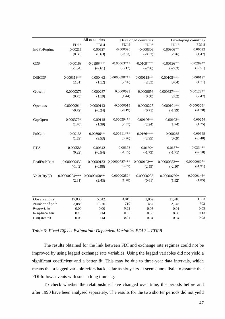
47
FDI 3 FDI 4 FDI 5 FDI 6 FDI 7 FDI 8
IndFixRegime 0.00215 0.00527 -0.000396 -0.000306 0.00306** 0.00622
(0.60) (0.63) (-0.63) (-0.32) (2.26) (1.47)
GDP -0.00168 -0.0156*** -0.00563*** -0.0109*** -0.00526** -0.0289**
(-1.34) (-2.61) (-3.12) (-2.96) (-2.03) (-2.51)
DiffGDP 0.000318** 0.000463 0.0000690*** 0.000118** 0.00105*** 0.00612*
(2.31) (1.12) (2.96) (2.33) (3.04) (1.71)
Growth 0.0000376 0.000287 0.0000533 0.0000656 0.000327*** 0.00122**
(0.75) (1.10) (1.44) (0.50) (2.82) (2.47)
Openess -0.00000914 -0.0000143 -0.0000019 0.0000227 -0.000101** -0.000309*
(-0.72) (-0.24) (-0.19) (0.71) (-1.99) (-1.78)
CapOpen 0.000379* 0.00118 0.000594** 0.00106** 0.00102* 0.00254
(1.76) (1.39) (2.57) (2.24) (1.74) (1.25)
PolCon 0.00138 0.00896** 0.00811*** 0.0166*** 0.000235 -0.00389
(1.52) (2.53) (3.26) (2.95) (0.09) (-0.40)
RTA 0.000583 -0.00342 -0.00378 -0.0130* -0.0157* -0.0334**
(0.22) (-0.54) (-1.55) (-1.73) (-1.71) (-2.10)
RealExchRate -0.000000439 -0.000001330.00000787*** 0.0000103** -0.00000352** -0.00000697*
(-1.42) (-0.98) (3.05) (2.55) (-2.30) (-1.91)
VolatilityER 0.00000204*** 0.00000458** 0.00000259* 0.00000233 0.00000769* 0.0000146*
(2.81) (2.43) (1.78) (0.61) (1.92) (1.85)
Observations 17,036 5,542 3,819 1,862 11,418 3,353
Number of pairid 3,085 1,276 710 457 2,145 802
R-sq-w ithin 0.00 0.00 0.02 0.05 0.01 0.03
R-sq-betw een 0.10 0.14 0.06 0.06 0.08 0.13
R-sq-overall 0.08 0.14 0.04 0.04 0.04 0.08
All countries Developed countries Developing countries
Table 6: Fixed Effects Estimation: Dependent Variables FDI 3 – FDI 8
The results obtained for the link between FDI and exchange rate regimes could not be
improved by using lagged exchange rate variables. Using the lagged variables did not yield a
significant coefficient and a better fit. This may be due to three-year data intervals, which
means that a lagged variable refers back as far as six years. It seems unrealistic to assume that
FDI follows events with such a long time lag.
To check whether the relationships have changed over time, the periods before and
after 1990 have been analysed separately. The results for the two shorter periods did not yield

48
a better fit or narrower confidence intervals for the coefficients. This indicates that the
influence of exchange rate regimes on FDI has been equally weak and spurious during the
more recent and the remote sampling period.
5 Concluding Remarks and Policy Implications
Over the last 20 years, FDI flows have surged and MNEs have become increasingly important
players in the world economy. Countries with economic problems and worsening financial
situations often turn to fixed exchange rate regimes as an emergency measure and as a
“lifebelt”. They do this because there is a widely held opinion that anchoring a weak currency
to a strong and important currency improves a country’s credibility and its standing with
potential foreign direct investors. As yet, there is little empirical evidence regarding the
validity of this assumption. This study tried to fill this gap by using data for a large sample of
countries, covering the period from 1978 to 2004.
The results obtained for the variables representing the exchange rate regime (with
direct and indirect pegs, respectively) were, with one exception, not significant. The empirical
results indicate a weak positive relationship between FDI flows and exchange rate regimes for
developing countries. The positive effects seem to be more robust if the share of FDI is used
as an explanatory variable. In this case, the relationship of the FDI variable with the sample,
including the observations where the missing FDI values were replaced by zeros, is
significant. The improved significance is most probably due to the spurious correlation
between the zero FDI values and the zeros of the exchange rate regime classification.
Therefore, the relationship seems to be weak and not robust. It is noteworthy for this
sample of developing countries, in contrast to that of developed and “all countries”, that all
coefficients of the direct and indirect exchange rate regime variables are in line with
expectations. This implies that for developing countries the imposition of exchange rate
regimes may have a small positive impact on FDI. But those results are only indicative at best
and are not robust. It is, therefore, of particular importance to note that the results do not
provide conclusive support for the imposition of fixed exchange rate regimes as a way to
attract FDI inflows in the wake of currency and economic crises. Politicians should rather rely
on other economic instruments to restore their countries’ stability and international credibility.
For developed countries, the results are inconclusive and not significant at all. In most
cases, the signs of the coefficients are even negative. This indicates that for developed
49
countries, imposing a fixed exchange rate regime in order to attract FDI flows is not a
dependable policy alternative.
Not surprisingly, the results for the “all countries” sample, comprising observations
for developed and developing countries are also not conclusive. Most of the coefficients are
positive, but none of them is significant. The sample of countries seems to be so
heterogeneous with regard to the relationship between FDI flows and the exchange rate
regime that it is not possible to draw clear conclusions.
For a few countries (e.g. China), fixed exchange rate regimes have coincided with high
FDI inflows, whereas the opposite was true for many other countries (like Ecuador).
Therefore, the casuistic evidence suggests that a country’s success inconsolidating its
economic position seems to depend to an overwhelming degree on factors other than a fixed
exchange rate regime.
On the other hand, it would be premature to completely dismiss the influence of the
exchange rate regime on FDI flows at this stage. To obtain a more reliable picture, it would be
useful to refine and improve the de facto exchange rate classification. As yet, there is no
method to validate the classification and the choice of the classification method is based on
subjective judgement. Also, the data sample comprises very heterogeneous countries and time
periods. It is highly likely that particular groups of countries were subject to certain regional
or political influences, which obscured the “true” situation. Those countries were lumped
together indiscriminately in the sample.
To make sure that these effects do not obliterate the results, it seems necessary to
investigate which events or circumstances shaped a country’s development in a particular way
and whether this had an influence on FDI flows. Reinhart and Rogoff‘s (2004) painstaking
analysis of de facto exchange rate regimes may serve as a good example. At the same time, it
shows how much work needs to be done in order to record the historical aspects and details of
each country’s economic development and to condense the findings into meaningful
indicators. These should subsequently be used as explanatory variables of FDI.
50
References Aizenman, J. (1992). Exchange Rate Flexibility, Volatility and Patterns of Domestic and
Foreign Direct Investment. IMF Staff Papers 39: 890-922.
Aizenman, J., and N. Marion (2001). The Merits of Horizontal versus Vertical FDI in the
Presence of Uncertainty. NBER Working Paper 8631. Cambridge, Mass. (National
Bureau of Economic Research).
Alesina, A., and A. Wagner (2003). Choosing (and Reneging on) Exchange Rate Regimes.
NBER Working Paper 9809. Cambridge, Mass. (Natinal Bureau of Economic
Research).
Amuedo-Dorantes, C., and S. Pozo (2001). Foreign Exchange Rates and Foreign Direct
Investment in the United States. International Trade Journal 15 (3): 323-343.
Anderson, J. E. (1979). A Theoretical Foundation for the Gravity Equation, American
Economic Review 69 (1): 106-116.
Barrel, R., Gottschalk, S., and S. Hall (2003). Foreign Direct Investment and Exchange Rate
Uncertainty in Imperfectly Competitive Industries. NIESR Discussion Paper 220.
London. (National Institute of Economic and Social Research).
(http://www.niesr.ac.uk/pubs/dps/Dp220.pdf).
Baxter, M., and M. A. Kouparitsas (2006). What Determines Bilateral Trade Flows? NBER
Working Paper 12188, Cambridge, Mass. (Natinal Bureau of Economic Research).
Bergstrand, J. H. (1985). The Gravity Equation in International Trade: Some Microeconomic
Foundations and Empirical Evidence. Review of Economics and Statistics 67 (3): 474-
481.
Bergstrand, J. H. (1989). The Generalized Gravity Equation, Monopolistic Competition and
the Factor-Proportions Theory in International Trade. Review of Economics and
Statistics 71 (1): 143-153.
Bénassy-Quéré, A., Fontagné, L., and A. Lahrèche-Révil (2001). Exchange Rate Strategies in
the Competition for Attracting Foreign Direct Investment. Journal of the Japanese and
International Economies 15 (2): 178-198.
Bloningen, B. A. (1997). Firm-Specific Assets and the Link between Exchange Rates and
Foreign Direct Investment. American Economic Review 87 (3): 447-465.
Bloningen, B. A. (2005). A review of the Empirical Literature on FDI Determinants. NBER
Working Papers 11299. Cambridge, Mass. (National Bureau of Economic Research).
51
Bubula, A., and I. Ötker-Robe (2002). The Evolution of Exchange Rate Regimes Since 1990:
Evidence from De Facto Policies. IMF Working Paper 02/155. Washington, DC.
(International Monetary Fund).
Bun, M. J. G., and F. J. G. M. Klaasen (2002). Has the Euro Increased Trade? Discussion
Paper 108 (2). Tinbergen Institute, Amsterdam.
Calvo, G. A., and C. M. Reinhart (2002). Fear of Floating. Quarterly Journal of Economics
117 (2): 379-408.
Campa, J. M., and L. S. Goldberg (1999). Investment, Pass-through and Exchange Rates: A
Cross-Country Comparison. International Economic Review 40 (2): 287-314.
Carr, D. L., Markusen, J. R., and K. E. Maskus (2001). Estimating the Knowledge-Capital
Model of the Multinational Enterprise. American Economic Review 91 (3): 693-708.
Caves, R. E. (1989). Exchange Rate Movements and Foreign Direct Investment in the United
States. In: Audretsch, D.B. and Claudon, M.P. (eds). The Internationalization of US
Markets. New York University Press, New York.
Chakrabarti, A. (2001). The Determinants of Foreign Direct Investment: Sensitivity Analyses
of Cross-Country Regressions. Kyklos 54 (1): 89-114.
Chinn, M. D., and H. Ito (2005). What Matters for Financial Development? Capital Controls,
Institutions, and Interactions, NBER Working Paper 11370. Cambridge, Mass. (National
Bureau of Economic Research).
Crowley, P., and J. Lee (2002). Exchange Rate Volatility and Foreign Investment:
International Evidence. International Trade Journal 17 (3): 227-252.
Cushman, D. O. (1985). Real Exchange Rate Risk, Expectations and the Level of Direct
Investment. Review of Economics and Statistics 67 (2): 297-308.
Cushman, D. O. (1988). Exchange Rate Uncertainty and Foreign Direct Investment in the
United States. Weltwirtschaftliches Archiv 124 (2): 322-335.
Cushman, D. O. (2001). Real Exchange Rate Risk, Expectations, and the Level of Direct
Investment. Review of Economics and Statistics 67 (2): 297-308
De Ménil, G. (1999). Real Capital Market Integration. Economic Policy 28: 165-201.
Dewenter, K. L. (1995). Do Exchange Rate Changes Drive Foreign Investment. Journal of
Business 68 (3): 405-433.
Diehl, M., and R. Schweickert (1997). Wechselkurspolitik im Aufholprozess: Erfahrungen
Lateinamerikanischer, Europäischer und Asiatischer Länder. Kieler Studien: 286. J.C.B.
Mohr, Tübingen.

52
Dixit, A. K., and R. S. Pindyck (1994). Investment under Uncertainty. Princeton University
Press, Princeton, NJ.
Dunning, J. H. (2001). The Eclectic (OLI) Paradigm of International Production: Past, Present
and Future. International Journal of Economics of Business 8 (2), 173-190.
Eichengreen, B. (1994). International Monetary Arrangements for the 21st Century.
Integrating National Economies, Washington DC.
Eichengreen, B., and S. Fischer (2001). Exchange Rate Regimes: Is the Bipolar View
Correct? Journal of Economic Perspectives 15 (2): 3-24.
Eichengreen, B., and R. Razo-Garcia (2006). The International Monetary System in the Last
and Next 20 Years. Economic Policy 47: 393-442, Oxford: Blackwell.
Esaka, T. (2007). De Facto Exchange Rate Regimes in Emerging Market Countries, 1990-
2001: Some Empirical Evidence. In: Mitsuo, H. (eds). New Developments of the
Exchange Rate Regimes in Developing Countries. Antony Rowe Ltd, Chippenham and
Eastborne: 8-58.
Eurostat (2005). European Union Foreign Direct Investment Yearbook 2005. Luxembourg
(European Communities).
Frankel, J. A. (1999). No Single Currency Regime is Right for all Countries or at all Times.
NBER Working Paper 7338, Cambridge, Mass. (National Bureau of Economic
Research).
Frankel, J., and A. Rose (2002). An Estimate of the Effect of Common Currencies on Trade
and Income. Quarterly Journal of Economics 117 (2): 437-466.
Froot, K. A., and J. C. Stein (1991). Exchange rates and foreign direct investment: An
imperfect capital markets approach. Quarterly Journal of Economics 106 (4): 1191-
1217.
Gast, M. (2005). Determinants of Foreign Direct Investment of OECD Countries 1991-2001.
Discussion Paper 27, Gießen. (Zentrum für Internationale Entwicklungs- und
Umweltforschung der Justus-Liebig-Universität Gießen). (http://www.uni-
giessen.de/zeu/Papers/DiscPap%2327.pdf).
Ghosh, A. R., Gulde, A. M., and H. C. Wolf (2002). Exchange Rate Regimes: Choices and
Consequences. MIT Press, Cambridge.
Goldberg, L. S., and C. D. Kolstad (1995). Foreign Direct Investment, Exchange Rate
Variability and Demand Uncertainty. International Economic Review 36 (4): 855-873.

53
Görg, H., and K. Wakelin (2002). The Impact of Exchange Rate Volatility on US Investment.
Manchester School 70 (3): 380-397.
Hausman, J. A. (1978). Specification Tests in Econometrics. Econometrica 46 (6): 1251-
1271.
Helpman, E. (1984). A Simple Theory of International Trade with Multinational
Corporations. Journal of Political Economy 92 (31): 451-471.
Henisz, W. (2000). The Institutional Environment for Multinational Investment. Journal of
Law, Economics and Organization 16 (2): 334-264.
Hubert, F., and N. Pain (1999). Innovation and the Regional and Industrial Pattern of German
Foreign Direct Investment. In: Barrell, R. and Pain, N. (eds.). Investment, Innovation
and the Diffusion of Technology in Europe. Cambridge University Press, Cambridge.
Itagaki, T. (1981). The Theory of the Multinational Firm under Exchange Rate Uncertainty.
Canadian Journal of Economics 14: 276-297.
Klein, M. W., and E. Rosengreen (1994). The Real Exchange Rate and Foreign Direct
Investment in the United States. Journal of International Economics 36 (3): 373-389.
Klein, M. W., and J. C. Shambaugh (2006). Fixed Exchange Rates and Trade. Journal of
International Economics 70 (2): 359-383.
Kogut, B., and S. J. Chang (1996). Platform Investments and Volatile Exchange Rates: Direct
Investment in the U.S. by Japanese Electronic Companies. Review of Economics and
Statistics 78 (2): 221-231.
Lafrance, R., and D. Tessier (2001). Exchange Rate Variability and Investment in Canada:
Revisiting the Case for Flexible Exchange Rates, Bank of Canada Conference
Proceedings, Bank of Canada.
Levy-Yeyati, E., Sturzenegger, F., and I. Reggio (2003). On the Endogeneity of Exchange
Rate Regimes. Universidad Torcuato Di Tella.
(http://200.32.4.58/~ely/endogeneity_revised.pdf).
Levy-Yeyati, E., and F. Sturzenegger (2005). Classifying Exchange Rate Regimes: Deeds vs.
words. European Economic Review 49 (6): 1603-1635.
Linnemann, H. (1966). An Econometric Study of International Trade Flows. North-Holland
Publishing Company, Amsterdam.
Lipsey, R. E. (2001). Foreign Direct Investors in Three Financial Crisis. NBER Working
Paper 8084. Cambridge, Mass. (National Bureau of Economic Research).

54
Markusen, J. R. (2002). Multinational Firms and the Theory of International Trade. MIT
Press, Cambridge.
Obstfeld, M., and K. Rogoff (1995). The Mirage of Fixed Exchange Rates. Journal of
Economic Perspectives 9 (4): 73-96.
Pain, N. (2003). Fiscal Policies, European Integration and Structural Changes in the Location
of German Foreign Direct Investment. In: Herrmann, H. and Lipsey, R. E. (eds) Foreign
Direct Investment in the Real and Financial Sector of Industrial Countries. Springer,
Berlin.
Pain, N., and D. Van Welsum (2003). Untying the Gordian Knot: The Multiple Links
Between Exchange Rates and Foreign Direct Investment. Journal of Common Market
Studies 41 (5); 823-846.
Petroulas, P. (2006). The Effect of the Euro on Foreign Direct Investment. Working Paper 48.
Bank of Greece, Athen.
Reinhart, C. M., and K. S. Rogoff (2003). FDI to Africa: The Role of Price Stability and
Currency Instability. IMF Working Paper No. WP/03/10. Washington DC.
(International Monetary Fund).
(http://www.imf.org/external/pubs/ft/wp/2003/wp0310.pdf).
Reinhart, C. M., and K. S. Rogoff (2004). The Modern History of Exchange Rate
Arrangements: a Reinterpretation. Quarterly Journal of Economics, Vol. 119 (1): 1-48.
Rose, A. (2000). One Money, one Market: The Effect of Common Currencies on Trade.
Economic Policy 30: 9-45.
Schiavo, S. (2005). Common Currencies and FDI Flows. LEM Working Paper Series
2005/07. Pisa. (Laboratory of Economics and Management).
(http://www.lem.sssup.it/WPLem/files/2005-07.pdf).
Shambaugh, J. C. (2004). The Effect of Fixed Exchange Rates on Monetary Policy. Quarterly
Journal of Economics 119 (1): 301-352
Stevens, G. V. G. (1998). Exchange Rate and Foreign Direct Investment: A Note. Journal of
Policy Modeling 20 (3): 393-401.
Stokman, A. C. J., and P. J. G. Vlaar (1996). Volatility, International Trade and Capital
Flows. In: Bruni, F., Fair, D. E. and O’Brein, R. (eds). Risk Management in Volatile
Financial Markets. Kluwer, Amsterdam.
Sung, H., and H. E. Lapan (2000). Strategic Foreign Direct Investment and Exchange Rate
Uncertainty. International Economic Review 41 (2): 411-423.
55
Tinbergen, J. (1962). Shaping the World Economy: Suggestions for an International
Economic Policy. Twentieth Century Fund, New York.
Tornell, A., and A. Velasco (2000). Fixed versus Flexible Exchange Rates: Which Provides
more Fiscal Discipline? Journal of Monetary Economics 45 (2): 399-436.
Udomkerdmongkolm, M., Görg, H., and O. Morrissey (2006). Foreign Direct Investment and
Exchange Rates: A Case Study of U.S. FDI in Emerging Market Countries. Discussion
Paper in Economics No. 06/05. University of Nottingham.
UNCTAD (2006). World Investment Report (2006). New York. (United Nations).
UNCTAD (2007a). Foreign Direct Investment Statistics (online database).
(http://www.unctad.org/Templates/Page.asp?intItemID=1923&lang=1).
UNCTAD (2007b). Foreign Direct Investment Statistics, Definitions and Sources.
(http://www.unctad.org/Templates/Page.asp?intItemID=3144&lang=1).
World Bank (2006). World Development Indicators 2006. Washington D. C.
(http://web.worldbank.org/WBSITE/EXTERNAL/DATASTATISTICS/0,,contentMDK:
20415471~menuPK:1192714~pagePK:64133150~piPK:64133175~theSitePK:239419,0
0.html).
WTO (2007). Regional Trade Agreements Internet Posting:
http://www.wto.org/english/tratop_e/region_e/region_e.htm

56
Appendix
Appendix A: Definition of Variables and Data Sources
Variable Definition Source
FDI 1 Bilateral FDI flows from source to host country in US$ million
UNCTAD (2007a)
FDI 2 Bilateral FDI flows from source to host country in US$ million, excluding missing value zeros UNCTAD (2007a)
FDI 3 Bilateral FDI flows from source to host country in % of total FDI to all countries included in our sample
UNCTAD (2007a)
FDI 4 Bilateral FDI flows from source to host country in % of total FDI to all countries included in our sample, excluding missing value zeros
UNCTAD (2007a)
FDI 5 Bilateral FDI flows from source to developed host country in % of total FDI to all developed countries included in our sample
UNCTAD (2007a)
FDI 6 Bilateral FDI flows from source to developed host country in % of total FDI to all developed countries included in our sample, excluding missing value zeros
UNCTAD (2007a)
FDI 7 Bilateral FDI flows from source to developing host country in % of total FDI to all developing countries included in our sample
UNCTAD (2007a)
FDI 8 Bilateral FDI flows from source to developing host country in % of total FDI to all developing countries included in our sample, excluding missing value zeros
UNCTAD (2007a)
FixRegime Indicator for fixed exchange rate regimes Reinhart and Rogoff (2004)
IndFixRegime Indicator for indirect fixed exchange rate regimes
Reinhart and Rogoff (2004)
GDP Real GDP, constant 2000 US$ World Bank (2006) DiffGDP Difference between source and host GDP per
capita, constant 2000 US$ World Bank (2006)
Growth Real GDP growth rate of host country in % World Bank (2006) Openness Sum of imports and exports in % of GDP (host
country) World Bank (2006)
RTA Dummy regional trade agreement, 0-1 WTO (2007) PolCon Political constraints III, Henisz database, 0-1 Downloaded from
Henisz’s homepage CapOpen Indicator for capital account openness; Chinn-Ito
index on financial openness Chinn and Ito (2005)
RealExchRate Real exchange rate against the US$ IMF (2007) VolatilityER Standard Deviation of the real exchange rate IMF (2007)

57
Appendix B: Source Country Sample
Argentina, Australia, Austria, Belgium-Luxembourg, Brazil, Canada, Chile, Colombia, Denmark, Finland, France, Germany, Iceland, Ireland, Japan, Republic of Korea, Malaysia, Mexico, Netherlands, New Zealand, Norway, Portugal, Spain, Sweden, Switzerland, Taiwan, Thailand, Turkey, United Kingdom, United States, Venezuela
Appendix C: Host Country Sample
Albania, Algeria, Angola, Argentina, Australia, Austria, Bangladesh, Belgium-Luxembourg, Bolivia, Botswana, Brazil, Bulgaria, Burkina Faso, Cameroon, Canada, Chile, China, Colombia, Republic of Congo, Costa Rica, Côte d'Ivoire, Croatia, Czech Republic, Denmark, Dominican Republic, Ecuador, Egypt, El Salvador, Equatorial Guinea, Estonia, Ethiopia, Finland, France, Gambia, Germany, Ghana, Greece, Guatemala, Guyana, Haiti, Honduras, Hungary, Iceland, India, Indonesia, Ireland, Israel, Italy, Japan, Jordan, Kazakhstan, Kenya, Republic of Korea, Latvia, Lithuania, Madagascar, Malaysia, Mali, Mauritius, Mexico, Mongolia, Morocco, Mozambique, Namibia, Netherlands, New Zealand, Nicaragua, Niger, Nigeria, Norway, Oman, Pakistan, Papua New Guinea, Paraguay, Peru, Philippines, Poland, Portugal, Romania, Russian Federation, Saudi Arabia, Senegal, Slovakia, Slovenia, Spain, Sri Lanka, Sudan, Swaziland, Sweden, Switzerland, Syrian Arab Republic, Taiwan, Tanzania, Thailand, Togo, Trinidad and Tobago, Tunisia, Turkey, Uganda, Ukraine, United Kingdom, United States, Uruguay, Venezuela, Vietnam, Zambia, Zimbabwe