Multilevel ModelingMultilevel Modeling
Soc 543Soc 543
Fall 2004Fall 2004

Presentation overviewPresentation overview
What is multilevel modeling?What is multilevel modeling?
Problems with not using multilevel modelsProblems with not using multilevel models
Benefits of using multilevel modelsBenefits of using multilevel models
Basic multilevel modelBasic multilevel model
Variation one: person and timeVariation one: person and time
Variation two: person, time, and spaceVariation two: person, time, and space

Multilevel modelsMultilevel models
Units of analysis are nested within higher-level Units of analysis are nested within higher-level units of analysisunits of analysis
Students within schoolsStudents within schools
Observations with personObservations with person

Problems without MLMProblems without MLM
If we ignore higher-level units of analysis => cannot If we ignore higher-level units of analysis => cannot account for context (individualistic approach) account for context (individualistic approach) If we ignore individual-level observation and rely on If we ignore individual-level observation and rely on higher-level units of analysis, we may commit ecological higher-level units of analysis, we may commit ecological fallacy (aggregated data approach)fallacy (aggregated data approach)Without explicit modeling, sampling errors at second Without explicit modeling, sampling errors at second level may be large =>unreliable slopeslevel may be large =>unreliable slopesHomoscedasticity and no serial correlation assumptions Homoscedasticity and no serial correlation assumptions of OLS are violated (an efficiency problem).of OLS are violated (an efficiency problem).No distinction between parameter and sampling No distinction between parameter and sampling variancesvariances

Advantages of MLMAdvantages of MLM
Cross-level comparisonsCross-level comparisons
Controls for level differencesControls for level differences

General MLMGeneral MLM
Example: Raudenbush and Bryk, 1986Example: Raudenbush and Bryk, 1986
Dependent variable: Dependent variable: ContinuousContinuous
ObservedObserved

General MLMGeneral MLM
High school and beyond (HSB) surveyHigh school and beyond (HSB) survey
10,231 students from 82 Catholic and 94 10,231 students from 82 Catholic and 94 public schools public schools
Dependent variable: standardized math Dependent variable: standardized math achievement scoreachievement score
Independent variable: SESIndependent variable: SES
General MLMGeneral MLM
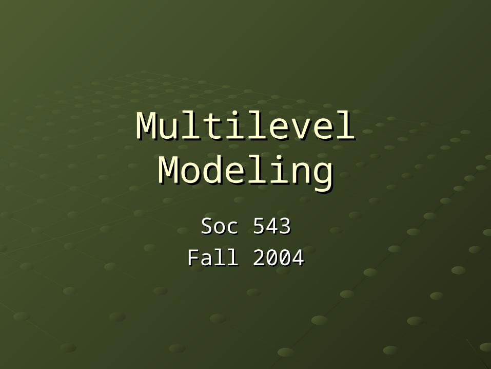
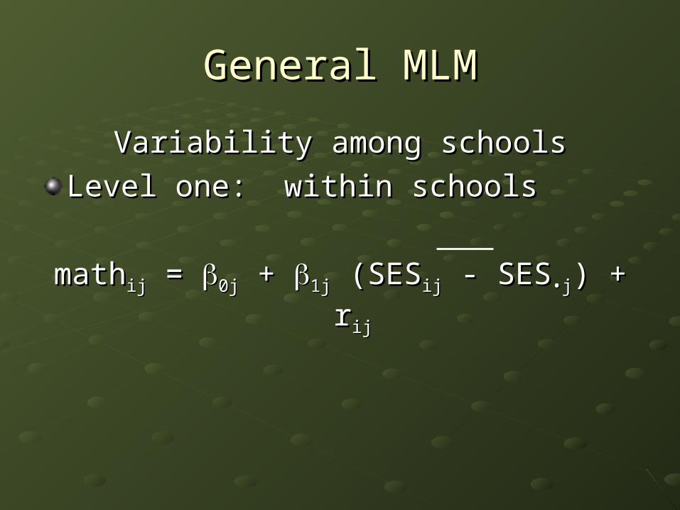
Variability among schoolsVariability among schools
Level one: within schoolsLevel one: within schools
mathmathijij = = 0j0j + + 1j1j (SES (SESijij - SES - SES•j•j) + r) + rijij

General MLMGeneral MLM
Variability among schoolsVariability among schools
Level two: between schoolsLevel two: between schools
0j0j = = 0000 + u + u0j0j
1j1j = = 1010 + u + u1j1j

General MLMGeneral MLM
Variability among schoolsVariability among schoolsCombined modelCombined model
mathmathijij = = 0000 + u + u0j0j + + 1010(SES(SESijij - SES - SES•j•j))+ u+ u1j1j(SES(SESijij - SES - SES•j•j) + r) + rijij = = 0000 + + 1010(SES(SESijij - SES - SES•j•j) ) + u+ u0j0j + v + vijij
(Easy interpretation given the “centering” (Easy interpretation given the “centering” parameterization)parameterization)

General MLMGeneral MLM
Variability among schoolsVariability among schools
Combined modelCombined model
mathmathijij = =
+ + (SES(SESijij - SES - SES•j•j))
+ u+ u0j0j + v + vijij
There is a positive relation between SES and There is a positive relation between SES and math scoremath score

General MLMGeneral MLM
Variability among schoolsVariability among schoolsResults: math score meansResults: math score means
school means are differentschool means are different90% of the variance is parameter variance90% of the variance is parameter variance10% is sampling variance10% is sampling variance
Results: math score-SES relationResults: math score-SES relationschool relations are differentschool relations are different35% is parameter variance (this requires 35% is parameter variance (this requires additional assumption and analysis)additional assumption and analysis)65% is sampling variance65% is sampling variance

General MLMGeneral MLM
Covariates at level 2 Covariates at level 2
Level one: within schoolsLevel one: within schools
mathmathijij = = 0j0j + + 1j1j (SES (SESijij - SES - SES•j•j) + r) + rijij

General MLMGeneral MLM
Covariates at level 2 Covariates at level 2
Level two: between schoolsLevel two: between schools
0j0j = = 0000 + + 0101sectsectjj+ u+ u0j0j
1j1j = = 1010 + + 1111sectsectjj+ u+ u1j1j

General MLMGeneral MLM
Covariates at level 2 Covariates at level 2
Combined model:Combined model:
mathmathijij = = 0000 + + 0101sectsectjj
+ + 10 10 SESSESijij - SES - SES•j•j) )
+ + 1111sectsectjj(SES(SESijij - SES - SES•j•j) )
+ r+ rij ij + v+ vjj
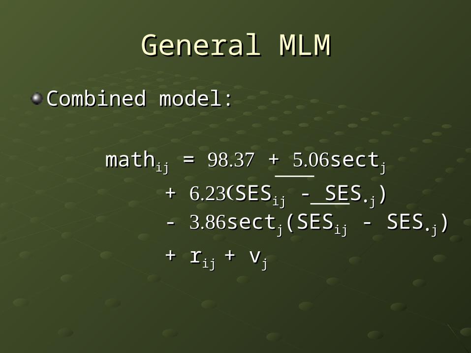
General MLMGeneral MLM
Combined model:Combined model:
mathmathijij = = + + sectsectjj
+ + SESSESijij - SES - SES•j•j) )
- - sectsectjj(SES(SESijij - SES - SES•j•j) )
+ r+ rij ij + v+ vjj

General MLMGeneral MLM
Variability as a function of sectorVariability as a function of sector
Results: math score meansResults: math score means80.7% is parameter variance80.7% is parameter variance
differences in school means is not entirely differences in school means is not entirely accounted for by sectoraccounted for by sector
Results: SES-math score relationResults: SES-math score relation9.7% is parameter variance9.7% is parameter variance
differences in school SES-math score differences in school SES-math score relation may be accounted for by sectorrelation may be accounted for by sector
General MLMGeneral MLM
Sector effectsSector effects
Cannot say that previous relations are Cannot say that previous relations are causal – may be selection effectscausal – may be selection effects
Use example of homework to explain Use example of homework to explain sector differencessector differences
General MLMGeneral MLM
Sector effectsSector effects
Results: Results: school SES is strongly related to mean school SES is strongly related to mean math score, but SES composition accounts math score, but SES composition accounts for Catholic differencefor Catholic difference
schools with lower SES had weaker SES-schools with lower SES had weaker SES-math score relation than higher SES math score relation than higher SES schoolsschools
General MLMGeneral MLM
Sector effectsSector effects
Results: Results: variation in SES-math score relation may variation in SES-math score relation may be accounted for by school SESbe accounted for by school SES
variation in mean math score is not entirely variation in mean math score is not entirely accounted for by school SESaccounted for by school SES
MLM with person and timeMLM with person and time
When observations are repeated for the When observations are repeated for the same units, we also have a nested same units, we also have a nested structure.structure.Examining within-person changes over Examining within-person changes over time – growth curve analysis. time – growth curve analysis. Growth curves may be similar across Growth curves may be similar across persons within a class.persons within a class.Example: Muthén and MuthénExample: Muthén and MuthénDependent variable: categorical, latentDependent variable: categorical, latent
Muthen and MuthenMuthen and Muthen
NLSYNLSY
N=7326 (part 1); N=924 (part 2); N=922 N=7326 (part 1); N=924 (part 2); N=922 (part 3); N=1225 (part 4)(part 3); N=1225 (part 4)
Dependent variables: antisocial behavior Dependent variables: antisocial behavior (excluding alcohol use) during past year, (excluding alcohol use) during past year, in 17 dichotomous items; alcohol use in 17 dichotomous items; alcohol use during past year, in 22 dichotomous itemsduring past year, in 22 dichotomous items

MLM with person and timeMLM with person and time
Part 1: latent class determination by latent Part 1: latent class determination by latent class analysis and factor analysisclass analysis and factor analysis
It’s a cross-sectional analysis of baseline It’s a cross-sectional analysis of baseline data in 1980.data in 1980.
It found 4 latent classes. It found 4 latent classes.
MLM with person and timeMLM with person and time
Part 2: growth curve determination by latent Part 2: growth curve determination by latent class growth curve analysis and growth mixture class growth curve analysis and growth mixture modelingmodelingIt uses longitudinal information.It uses longitudinal information.Different growth curves are allowed and Different growth curves are allowed and estimated for different latent classes.estimated for different latent classes.Growth mixture modeling is a generalization of Growth mixture modeling is a generalization of latent class growth analysis, in allowing growth latent class growth analysis, in allowing growth variance within classvariance within classGMM yields a 4-class solution. GMM yields a 4-class solution.

MLM with person and timeMLM with person and time
Part 3: latent class relation to growth Part 3: latent class relation to growth curve model by general growth mixture curve model by general growth mixture modeling (GGMM)modeling (GGMM)What’s new is to the ability to predict a What’s new is to the ability to predict a categorical outcome variable from latent categorical outcome variable from latent classes. classes. The example also illustrates how The example also illustrates how covariates that predict membership in covariates that predict membership in classes (Table 4). classes (Table 4).
MLM with person and timeMLM with person and time
Part 4: latent class relation to growth curve Part 4: latent class relation to growth curve model by GGMMmodel by GGMM
Multiple (2) latent class variables.Multiple (2) latent class variables.
The first one comes from Part 1; the second The first one comes from Part 1; the second one comes from Part 2. one comes from Part 2.
It bridges the two component parts, asking It bridges the two component parts, asking how the first class membership affects how the first class membership affects membership in the second class scheme. membership in the second class scheme.

MLM with person, time & spaceMLM with person, time & space
Example: Axinn and YabikuExample: Axinn and Yabiku
Dependent variable: dichotomous, Dependent variable: dichotomous, observedobserved
Hazard model with event historyHazard model with event history
MLM with person, time & spaceMLM with person, time & space
Chitwan Valley Family Study (CVFS)Chitwan Valley Family Study (CVFS)
171 neighborhoods (5-15 household 171 neighborhoods (5-15 household cluster)cluster)
Dependent variable: initiated Dependent variable: initiated contraception to terminate childbearingcontraception to terminate childbearing

MLM with person, time & spaceMLM with person, time & space
Age 0 Age 12 Birth of 1st child
Contraceptive use or end of observation
Time-invariant childhood community context
Time-varying contemporary community context
Time-invariant early life nonfamily experiences
Time-varying contemporary nonfamily experiences

MLM with person, time & spaceMLM with person, time & space
Level one:Level one:
Logit(pLogit(ptijtij) = ) = 0j0j + + 11CCjj+ + 2XXij + +3DDjt + + 4ZZijt
C: time-invariant community var. C: time-invariant community var.
D: time-variant community var.D: time-variant community var.
X: time-invariant personal var.X: time-invariant personal var.
Z: time-variant personal var.Z: time-variant personal var.
(Note that there is no interaction across (Note that there is no interaction across levels)levels)

Multi-level Hazard ModelsMulti-level Hazard Models
There is a general problem with non-linear There is a general problem with non-linear multi-level models.multi-level models.Unbiasedness breaks down. Unbiasedness breaks down.
Special attention needs to be paid to Special attention needs to be paid to estimation of hazard models in a multi-estimation of hazard models in a multi-level setting.level setting.
See Barber et al (2000). See Barber et al (2000).