Multilevel Modeling Recent Developments in Multilevel Modeling Roberto G. Gutierrez Director of Statistics StataCorp LP 2007 Nordic and Baltic Stata Users Group Meeting, Stockholm R. Gutierrez (StataCorp) September 7, 2007 1 / 32

Welcome message from author
This document is posted to help you gain knowledge. Please leave a comment to let me know what you think about it! Share it to your friends and learn new things together.
Transcript

Multilevel Modeling
Recent Developments in Multilevel Modeling
Roberto G. Gutierrez
Director of StatisticsStataCorp LP
2007 Nordic and Baltic Stata Users Group Meeting, Stockholm
R. Gutierrez (StataCorp) September 7, 2007 1 / 32

Multilevel Modeling
Outline
1. What’s new in Stata 10
2. One-level models
3. Alternate covariance structures
4. A two-level model
5. The Laplacian approximation
6. A crossed-effects model
7. Concluding remarks
R. Gutierrez (StataCorp) September 7, 2007 2 / 32

Multilevel Modeling
What’s new in Stata 10
New commands xtmelogit and xtmepoisson
Mixed effects for binary and count responses
They work just like xtmixed does
Random intercepts and random coefficients
You can have multiple levels of nested random effects
Various predictions, including random effects and theirstandard errors
We’ll be discussing binary responses and xtmelogit
R. Gutierrez (StataCorp) September 7, 2007 3 / 32

Multilevel Modeling
One-level models
Definition
For a series of i = 1, . . . ,M independent panels, let
P(yij = 1|ui) = H(xijβ + zijui)
where
there are j = 1, . . . , nij observations in panel i
xij are the p covariates for the fixed effects
β are the fixed effects
zij are the q covariates for the random effects
ui are the random effects, specific to panel i
ui are normal with mean 0 and variance matrix Σ
H() is the logistic cdf
R. Gutierrez (StataCorp) September 7, 2007 4 / 32

Multilevel Modeling
One-level models
Alternate formulation
You can also think of this model in terms of a latent responseyij = I (y∗
ij > 0) where
y∗
ij = xijβ + zijui + ǫij
The errors ǫij are logistic-distributed with mean zero andvariance π2/3, independent of ui
R. Gutierrez (StataCorp) September 7, 2007 5 / 32

Multilevel Modeling
One-level models
Variance Components
Random effects are not directly estimated, but insteadcharacterized by the elements of Σ, known as variance
components
You can, however, “predict” random effects
As such, you fit this model by estimating β and the variancecomponents in Σ
A maximum-likelihood solution requires integrating out thedistribution of ui .
A tricky proposition in nonlinear models such as logit
R. Gutierrez (StataCorp) September 7, 2007 6 / 32

Multilevel Modeling
One-level models
Bangladesh fertility survey
Example
1989 Bangladesh fertility survey (Huq and Cleland 1990)
Ng et al. (2006) analyze data on 1,934 women, who werepolled on their use of contraception
Data were collected from 60 districts containing urban andrural areas
Covariates include age, urban/rural area, and indicators fornumber of children
Among other things, we wish to assess a district effect oncontraception use
R. Gutierrez (StataCorp) September 7, 2007 7 / 32
Multilevel Modeling
One-level models
Modeling contraception use
For woman j in district i , consider this model forπij = P(c useij = 1)
logit(πij) = β0 + β1urbanij + β2ageij +
β3child1ij + β4child2ij + β5child3ij + ui
The ui represent 60 district-specific random effects
You can use xtlogit (option re) to fit this model andestimate σ2
u, the variance of the ui
xtlogit will also give an LR test for Ho : σ2u = 0, by
comparing log likelihoods with logit
You could also use xtmelogit on this model
R. Gutierrez (StataCorp) September 7, 2007 8 / 32

Multilevel Modeling
One-level models
Stretching our wings
Introducing a random coefficient, we now consider
logit(πij ) = β0 + β1urbanij + Fij + ui+viurbanij
Fij is shorthand for the fixed-effects specification on age andchildren
This model allows for distinct random effects for urban andrural areas within each district
For rural areas in district i , the effect is ui
For urban areas, ui + vi
You need xtmelogit to fit this model
R. Gutierrez (StataCorp) September 7, 2007 9 / 32

Multilevel Modeling
One-level models
Using xtmelogit
. xtmelogit c_use urban age child* || district: urban
Refining starting values:
(output omitted )
Performing gradient-based optimization:
(output omitted )
Mixed-effects logistic regression Number of obs = 1934
Group variable: district Number of groups = 60
Obs per group: min = 2avg = 32.2
max = 118
Integration points = 7 Wald chi2(5) = 97.30Log likelihood = -1205.0025 Prob > chi2 = 0.0000
c_use Coef. Std. Err. z P>|z| [95% Conf. Interval]
urban .7143927 .1513595 4.72 0.000 .4177336 1.011052
age -.0262261 .0079656 -3.29 0.001 -.0418384 -.0106138child1 1.128973 .1599346 7.06 0.000 .8155069 1.442439
child2 1.363165 .1761804 7.74 0.000 1.017857 1.708472child3 1.352238 .1815608 7.45 0.000 .9963853 1.70809_cons -1.698137 .1505019 -11.28 0.000 -1.993115 -1.403159
--more--
R. Gutierrez (StataCorp) September 7, 2007 10 / 32

Multilevel Modeling
One-level models
Using xtmelogit
Random-effects Parameters Estimate Std. Err. [95% Conf. Interval]
district: Independentsd(urban) .5235464 .203566 .2443374 1.121813
sd(_cons) .4889585 .087638 .3441182 .6947624
LR test vs. logistic regression: chi2(2) = 47.05 Prob > chi2 = 0.0000
Note: LR test is conservative and provided only for reference.
R. Gutierrez (StataCorp) September 7, 2007 11 / 32
Multilevel Modeling
One-level models
Some notes
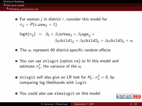
As with logit, option or will give odds ratios
Use option variance for variances instead of standarddeviations of random effects
LR test comparing to standard logit is at the bottom, alongwith a note telling you the p-value is conservative
R. Gutierrez (StataCorp) September 7, 2007 12 / 32

Multilevel Modeling
One-level models
Revisiting that tricky proposition
Evaluating the log likelihood requires integrating out therandom effects
The default method used by xtmelogit is adaptive Gaussianquadrature (AGQ) with seven quadrature points per level
AGQ is computationally intensive
Previous methods, such as PQL and MQL, avoided theintegration altogether (Breslow and Clayton 1993)
PQL and MQL can be severely biased (Rodriguez andGoldman 1995)
Also, being quasi-likelihood, their use prohibits LR tests
R. Gutierrez (StataCorp) September 7, 2007 13 / 32

Multilevel Modeling
Alternate covariance structures
Extending the model
Implicit in our previous model was the default independentcovariance structure
Σ = Var
[
ui
vi
]
=
[
σ2u 00 σ2
v
]
Assuming Cov(ui , vi ) = 0 means you are also assumingVar(ui + vi ) > Var(ui )
Are urban areas really more variable than rural areas?
Even worse, what if we change the coding of the randomeffects? Codings are not arbitrary here
Option covariance(unstructured) will include thiscovariance in the model
R. Gutierrez (StataCorp) September 7, 2007 14 / 32
Multilevel Modeling
Alternate covariance structures
Unstructured covariance
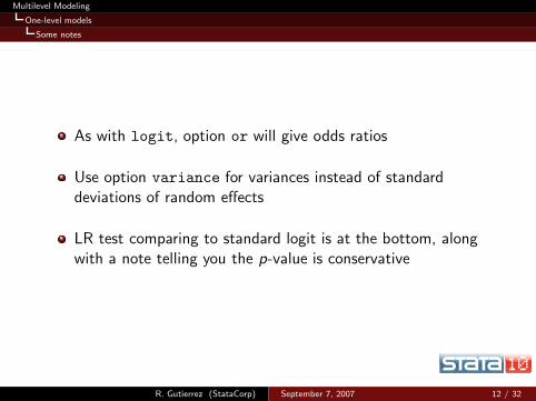
. xtmelogit c_use urban age child* || district: urban, cov(un) var
(output omitted )
Mixed-effects logistic regression Number of obs = 1934Group variable: district Number of groups = 60
Obs per group: min = 2
avg = 32.2max = 118
Integration points = 7 Wald chi2(5) = 97.50
Log likelihood = -1199.315 Prob > chi2 = 0.0000
c_use Coef. Std. Err. z P>|z| [95% Conf. Interval]
urban .8157872 .1715519 4.76 0.000 .4795516 1.152023age -.026415 .008023 -3.29 0.001 -.0421398 -.0106902
child1 1.13252 .1603285 7.06 0.000 .818282 1.446758child2 1.357739 .1770522 7.67 0.000 1.010724 1.704755
child3 1.353827 .1828801 7.40 0.000 .9953882 1.712265_cons -1.71165 .1605617 -10.66 0.000 -2.026345 -1.396954
--more--
R. Gutierrez (StataCorp) September 7, 2007 15 / 32
Multilevel Modeling
Alternate covariance structures
Unstructured covariance
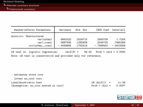
Random-effects Parameters Estimate Std. Err. [95% Conf. Interval]
district: Unstructured
var(urban) .6663222 .3224715 .2580709 1.7204var(_cons) .3897435 .1292459 .2034723 .7465388
cov(urban,_cons) -.4058846 .1755418 -.7499403 -.0618289
LR test vs. logistic regression: chi2(3) = 58.42 Prob > chi2 = 0.0000
Note: LR test is conservative and provided only for reference.
. estimates store corr
. lrtest no_corr corr
Likelihood-ratio test LR chi2(1) = 11.38(Assumption: no_corr nested in corr) Prob > chi2 = 0.0007
R. Gutierrez (StataCorp) September 7, 2007 16 / 32

Multilevel Modeling
Alternate covariance structures
Recoding your random effects
We can now estimate the variance of the random effects forurban areas as
Var(ui + vi) = σ2u + σ2
v + 2σuv
If you did this, you would get Var(ui + vi) = 0.244, which isactually less than Var(ui ) = 0.390
Better still, if you want to directly compare rural areas tourban areas, recode your random effects
The unstructured covariance structure will ensure anequivalent model under alternate codings of random-effectsvariables
Also, predictions of random effects will be what you want
R. Gutierrez (StataCorp) September 7, 2007 17 / 32
Multilevel Modeling
Alternate covariance structures
Recoding your random effects
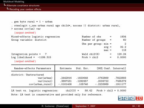
. gen byte rural = 1 - urban
. xtmelogit c_use urban rural age child*, nocons || district: urban rural,> nocons cov(un) var
(output omitted )
Mixed-effects logistic regression Number of obs = 1934
Group variable: district Number of groups = 60
Obs per group: min = 2avg = 32.2max = 118
Integration points = 7 Wald chi2(6) = 120.24
Log likelihood = -1199.315 Prob > chi2 = 0.0000
(output omitted )
Random-effects Parameters Estimate Std. Err. [95% Conf. Interval]
district: Unstructured
var(urban) .2442916 .1450648 .0762869 .7822893var(rural) .3897431 .1292457 .2034722 .7465379
cov(urban,rural) -.0161406 .105746 -.2233989 .1911177
LR test vs. logistic regression: chi2(3) = 58.42 Prob > chi2 = 0.0000
Note: LR test is conservative and provided only for reference.
R. Gutierrez (StataCorp) September 7, 2007 18 / 32

Multilevel Modeling
Alternate covariance structures
Compound Structures
You’ve seen Independent and Unstructured in action
Also available are Identity and Exchangeable
You can combine these to form blocked-diagonal structures
Such structures can reduce the number of estimableparameters
For example, consider a random effects specification of theform
... || district: child1 child2, nocons cov(ex) || district: child3, nocons
as an alternative to a 3 × 3 unstructured variance matrix
R. Gutierrez (StataCorp) September 7, 2007 19 / 32
Multilevel Modeling
A two-level model
The Tower of London
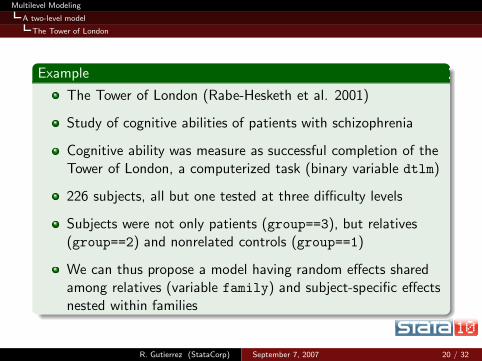
Example
The Tower of London (Rabe-Hesketh et al. 2001)
Study of cognitive abilities of patients with schizophrenia
Cognitive ability was measure as successful completion of theTower of London, a computerized task (binary variable dtlm)
226 subjects, all but one tested at three difficulty levels
Subjects were not only patients (group==3), but relatives(group==2) and nonrelated controls (group==1)
We can thus propose a model having random effects sharedamong relatives (variable family) and subject-specific effectsnested within families
R. Gutierrez (StataCorp) September 7, 2007 20 / 32

Multilevel Modeling
A two-level model
The Tower of London
. xi: xtmelogit dtlm difficulty i.group || family: || subject:, or variance
i.group _Igroup_1-3 (naturally coded; _Igroup_1 omitted)
(output omitted )
Mixed-effects logistic regression Number of obs = 677
No. of Observations per Group Integration
Group Variable Groups Minimum Average Maximum Points
family 118 2 5.7 27 7
subject 226 2 3.0 3 7
Wald chi2(3) = 74.89
Log likelihood = -305.12043 Prob > chi2 = 0.0000
dtlm Odds Ratio Std. Err. z P>|z| [95% Conf. Interval]
difficulty .192337 .0371622 -8.53 0.000 .131704 .2808839_Igroup_2 .7798295 .2763766 -0.70 0.483 .3893394 1.561964
_Igroup_3 .3491338 .1396499 -2.63 0.009 .1594117 .7646517
--more--
R. Gutierrez (StataCorp) September 7, 2007 21 / 32

Multilevel Modeling
A two-level model
The Tower of London
Random-effects Parameters Estimate Std. Err. [95% Conf. Interval]
family: Identityvar(_cons) .569182 .5216584 .0944322 3.430694
subject: Identityvar(_cons) 1.137931 .6857497 .3492672 3.707441
LR test vs. logistic regression: chi2(2) = 17.54 Prob > chi2 = 0.0002
Note: LR test is conservative and provided only for reference.
R. Gutierrez (StataCorp) September 7, 2007 22 / 32

Multilevel Modeling
The Laplacian approximation
Computation time
xtmelogit, by default, uses AGQ which can be intensive withlarge datasets or high-dimensional models
Computation time is roughly on the order of
T ∼ p2{M + M(NQ)qt}
where
p is the number of estimable parametersM is the number of lowest-level (smallest) panelsNQ is the number of quadrature pointsqt is the total dimension of the random effects (all levels)
The real killer is (NQ)qt
R. Gutierrez (StataCorp) September 7, 2007 23 / 32

Multilevel Modeling
The Laplacian approximation
Option laplace
Ideally, you want enough quadrature points such that addingmore points doesn’t change much
In complex models, this can very time consuming, especiallyduring the exploratory phase of the analysis
Sometimes you just want quicker results, and you may bewilling to give up a bit of accuracy
Use option laplace, equivalent to NQ = 1
The computational benefit is clear – one raised to any powerequals one
R. Gutierrez (StataCorp) September 7, 2007 24 / 32
Multilevel Modeling
The Laplacian approximation
Option laplace
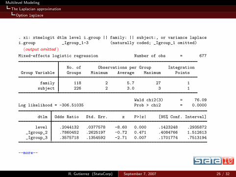
. xi: xtmelogit dtlm level i.group || family: || subject:, or variance laplace
i.group _Igroup_1-3 (naturally coded; _Igroup_1 omitted)
(output omitted )
Mixed-effects logistic regression Number of obs = 677
No. of Observations per Group Integration
Group Variable Groups Minimum Average Maximum Points
family 118 2 5.7 27 1
subject 226 2 3.0 3 1
Wald chi2(3) = 76.09
Log likelihood = -306.51035 Prob > chi2 = 0.0000
dtlm Odds Ratio Std. Err. z P>|z| [95% Conf. Interval]
level .2044132 .0377578 -8.60 0.000 .1423248 .2935872_Igroup_2 .7860452 .2625197 -0.72 0.471 .4084766 1.512613
_Igroup_3 .3575718 .1354592 -2.71 0.007 .1701774 .7513194
--more--
R. Gutierrez (StataCorp) September 7, 2007 25 / 32
Multilevel Modeling
The Laplacian approximation
Option laplace
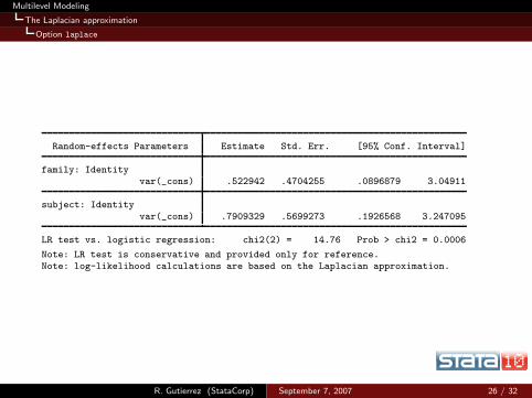
Random-effects Parameters Estimate Std. Err. [95% Conf. Interval]
family: Identityvar(_cons) .522942 .4704255 .0896879 3.04911
subject: Identity
var(_cons) .7909329 .5699273 .1926568 3.247095
LR test vs. logistic regression: chi2(2) = 14.76 Prob > chi2 = 0.0006
Note: LR test is conservative and provided only for reference.Note: log-likelihood calculations are based on the Laplacian approximation.
R. Gutierrez (StataCorp) September 7, 2007 26 / 32

Multilevel Modeling
The Laplacian approximation
Option laplace
Odds ratios and their standard errors are well approximated byLaplace
Variance components exhibit bias, particularly at the lower(subject) level
Model log-likelihoods and comparison LR test are in fairagreement
These behaviors are fairly typical
If anything, it shows that you can at least use laplace whilebuilding your model
R. Gutierrez (StataCorp) September 7, 2007 27 / 32

Multilevel Modeling
A crossed-effects model
Fife
One further advantage of laplace is that it permits you to fitcrossed-effects models, which will have high-dimension
Example
School data from Fife, Scotland (Rabe-Hesketh and Skrondal2005)
Attainment scores at age 16 for 3,435 students who attendedany of 148 primary schools and 19 secondary schools
We are interested in whether the attainment score is greaterthan 6
We want random effects due to primary school and secondaryschool, but these effects are not nested
R. Gutierrez (StataCorp) September 7, 2007 28 / 32

Multilevel Modeling
A crossed-effects model
Model
Consider the model
logit{(Pr(attainijk > 6)} = β0 + β1sexijk + ui + vj
for student k who attended primary school i and secondaryschool j
Since there is no nesting, you can use the level designationall: to treat the entire data as one big panel
Use factor notation R.varname to mimic the creation ofindicator variables identifying schools
However, notice that we can treat one set of effects as nestedwithin the entire data
R. Gutierrez (StataCorp) September 7, 2007 29 / 32

Multilevel Modeling
A crossed-effects model
Estimation results
. xtmelogit attain_gt_6 sex || _all:R.sid || pid:, or variance
Note: factor variables specified; option laplace assumed
(output omitted )
Mixed-effects logistic regression Number of obs = 3435
No. of Observations per Group Integration
Group Variable Groups Minimum Average Maximum Points
_all 1 3435 3435.0 3435 1pid 148 1 23.2 72 1
Wald chi2(1) = 14.28
Log likelihood = -2220.0035 Prob > chi2 = 0.0002
attain_gt_6 Odds Ratio Std. Err. z P>|z| [95% Conf. Interval]
sex 1.32512 .0986968 3.78 0.000 1.145135 1.533395
--more--
R. Gutierrez (StataCorp) September 7, 2007 30 / 32

Multilevel Modeling
A crossed-effects model
Estimation results
Random-effects Parameters Estimate Std. Err. [95% Conf. Interval]
_all: Identityvar(R.sid) .1239739 .0694743 .0413354 .3718252
pid: Identity
var(_cons) .4520502 .0953867 .298934 .6835937
LR test vs. logistic regression: chi2(2) = 195.80 Prob > chi2 = 0.0000
Note: LR test is conservative and provided only for reference.Note: log-likelihood calculations are based on the Laplacian approximation.
R. Gutierrez (StataCorp) September 7, 2007 31 / 32

Multilevel Modeling
Concluding remarks
xtmelogit and xtmepoisson are new to Stata 10
We discussed xtmelogit – the same holds true forxtmepoisson
Computations can get intensive
The Laplacian approximation is a quicker alternative
You can fit crossed-effects models, and large ones withcreative nesting
Work in this area is ongoing
R. Gutierrez (StataCorp) September 7, 2007 32 / 32

Multilevel Modeling
References
Breslow, N. E. and D. G. Clayton. 1993. Approximate inference in generalized linear mixed models. Journal of theAmerican Statistical Association 88: 9–25.
Huq, N. M. and J. Cleland. 1990. Bangladesh Fertility Survey 1989 (Main Report). National Institute ofPopulation Research and Training.
Ng, E. S. W., J. R. Carpenter, H. Goldstein, and J. Rasbash. 2006. Estimation in generalised linear mixed modelswith binary outcomes by simulated maximum likelihood. Statistical Modelling 6: 23–42.
Rabe-Hesketh, S., S. R. Touloupulou, and R. M. Murray. 2001. Multilevel modeling of cognitive function inschizophrenics and their first degree relatives. Multivariate Behavioral Research 36: 279–298.
Rabe-Hesketh, S. and A. Skrondal. 2005. Multilevel and Longitudinal Modeling Using Stata. College Station, TX:Stata Press.
Rodriguez, G. and N. Goldman. 1995. An assessment of estimation procedures for multilevel models with binaryresponses. Journal of the Royal Statistical Society, Series A 158: 73–89.
R. Gutierrez (StataCorp) September 7, 2007 32 / 32
Related Documents