Tuck School of Business at Dartmouth
Working Paper No.02-03
January 6, 2003
Monotonicity in Direct RevelationMechanisms
Diego GarciaTuck School of Business at Dartmouth
This paper can be downloaded from theSocial Science Research Network Electronic Paper Collection:
http://papers.ssrn.com/abstract_id=299569
Monotonicity in Direct Revelation Mechanisms∗
Diego Garcıa†
Amos Tuck School of Business Administration, Dartmouth College
January 6, 2003
∗I would like to thank Robert G. Hansen, Eric Rasmusen and participants at the North AmericanSummer Meeting of the Econometric Society (UCLA, 2002) for their comments.
†Correspondence information: Diego Garcıa, Tuck School of Business at Dartmouth, Hanover NH03755-9000, tel: (603) 646-3615, fax: (603) 646-1308, email: [email protected].
1
Abstract
This paper studies a standard mechanism design problem where the principal’s
allocation rule is multi-dimensional, and the agent’s private information is a one-
dimensional continuous variable. Under standard assumptions, that guarantee
monotonicity of the allocation rule in one-dimensional mechanisms, it is shown
that the optimal allocation will be non-monotonic in a (weakly) generic sense once
the principal can use all screening variables. The paper further gives conditions on
the model’s parameters that guarantee that non-monotonic allocation rules will be
optimal. It is shown that either (1) a total surplus function with negative cross-
partial derivatives, or (2) a marginal utility (with respect to information) for the
agent with positive cross-partial derivatives, can generate optimal non-monotonic
allocation rules.
JEL classification: C70, D82.
Keywords: multi-dimensional allocation rules, mechanism design, monotonic-
ity.
2
1 Introduction
Since the seminal work of Mirrlees (1971), economists have developed a tremendous
amount of insights into the behavior of agents facing asymmetric information. It is a
well established fact that the implementability of different allocation rules is hindered
by the presence of private information. Among the typical examples of the literature are
the problems faced by a monopolist that designs a non-linear pricing schedule (Mussa
and Rosen (1978)), a government contracting with a privately informed firm (Baron
and Myerson (1982)), an auctioneer trying to decide on a set of auction rules (Myer-
son (1981)), and headquarters designing a capital budgeting process (Harris, Kriebel,
and Raviv (1982)). One of the key results from these type of models is that there is
a monotonic distortion in the allocation rule: agents with higher values of the private
information receive a higher allocation of the good. This monotonicity result is an imme-
diate consequence of incentive compatibility when the allocation rule is one-dimensional.
The importance of this result cannot be overstated, since this qualitative prediction of
the model is its main empirical implication: a positive relationship between private
information and the allocation rule.
Much attention has been devoted lately to the standard monopolistic screening prob-
lem with multi-dimensional types (see Rochet and Stole (2000) for a review of the lit-
erature). Somewhat less attention has actually been devoted to the problem where the
asymmetric information faced by the principal is one-dimensional, but allocation rules
may be multi-dimensional.1 For example, in a non-linear pricing problem, the monop-
olist may not just consider the quantity schedule to be given to the agents (and its
corresponding price), but also the quality of the product. In a capital budgeting prob-
1In the literature surveyed by Rochet and Stole (2000) the standard model has a set of n differentscreening variables with n-dimensional private information, of which the setting in this paper is a specialcase. The main focus of this literature is in dealing with the difficulties that the multi-dimensional natureof the informational rents brings to the problem, since it is difficult to find what direction the incentivecompatibility constraint will bind.
3
lem, headquarters may not want to just decide on the investment amount to be delegated
down to each division, but also on the compensation scheme that each manager should
face.2 Mirman and Sibley (1980) were among the first to consider this type of problem.3
Their paper noted that the principal’s problem boils down to offering a one-dimensional
“menu path,” as a consequence of the revelation principle. This in turn implies that
standard techniques can be used to solve the model.4 The authors assumed that each
variable was monotonically related to private information, as in the one-dimensional
model,5 although they noted that there are no “precise conditions” under which this
monotonicity will be a result of the principal’s optimization problem.6
The paper by Matthews and Moore (1987) tackled this problem in a general model
with discrete-types. They consider a setting in which a monopolist is discriminating
both along a quality dimension and using warranties on the product. With a three-
type example they are able to show that quality may not be monotone in the private
information of the agent.7 The purpose of this paper is to understand and give conditions
under which non-monotonic allocation rules may be optimal in a setting where agents
have quasi-linear preferences. I study the standard “textbook model” (see Fudenberg
and Tirole (1991) or Stole (1997)), which subsumes many of the models in the literature,
2See Bernardo, Cai, and Luo (2001) for an agency model with private information where thesetwo elements are present. In contrast to the cases considered in this paper, the model studied byBernardo, Cai, and Luo (2001) exhibits monotone investment and compensation schemes. Besanko andSibley (1991) also present a model with multiple screening variables, in a transfer-pricing setting, wheremonotonicity is present in their optimal solutions.
3The literature that deals with “bundling” of goods is obviously related (e.g. Spence (1980)), althoughthe focus in this literature is significantly different than the issues addressed here. See also Roberts(1979).
4It is worth noticing that the problem with multiple screening variables and one-dimensional in-formational asymmetry is much easier at a technical level than the problem in which the types of theinformed party are multi-dimensional. This is due to the fact that the incentive-compatibility constraintis still a one-dimensional constraint, and it is straightforward to put enough structure in the problemso as to make sure the incentive compatibility constraints only bind in one direction.
5See equation (3) in p. 662.6The characterization of implementable allocations in Guesnerie and Laffont (1984) also restricts the
sufficiency conditions for implementability to monotonic allocation rules.7Another example of this non-monotonicity result, in a similar model to that in Matthews and Moore
(1987), is provided in van Egteren (1996).
4
under conditions that guarantee that a local approach, one in which only the downward
incentive-compatibility constraints bind, is valid. It is shown that under reasonable
conditions it will be (weakly) generically optimal for the principal to have non-monotonic
allocation rules, a result of the same flavor as the one in Matthews and Moore (1987).8
The paper further studies conditions under which the optimal allocation will be non-
monotonic. It is shown that either (1) a total surplus function with negative cross-partial
derivatives, or (2) a marginal utility (with respect to information) for the agent with
positive cross-partial derivatives can generate optimal non-monotone allocation rules. It
is worth noticing that in case (1), which allows for the allocation in a first-best world to
be decreasing, it is possible for the optimal allocation to be decreasing over the whole
range of realizations of private information for the agent. This may be optimal even
when in a model where this would be the only element of the allocation rule the optimal
mechanism would involve a strictly increasing allocation.
In the model studied both parties have quasi-linear preferences. It is also assumed
that the single-crossing property holds for each variable in isolation (i.e. holding all other
elements of the allocation vector constant). This, together with standard assumptions
on the model (such as a monotone hazard ratio for the distribution of the private infor-
mation), guarantees that if the principal could only use one screening variable, then the
optimal allocation will be increasing in the type of the agent. The main result of the
paper concerns the case where the principal can use the full vector of allocations to dis-
criminate among agents. It is shown that in a (weakly) generic sense the monotonicity
property of one-dimensional models breaks down: it is possible for some elements of the
optimal allocation to be non-monotonic in the agent’s type at the optimal solution.9
The paper extends the sufficient conditions given in Guesnerie and Laffont (1984) in
8By weak genericity I mean that a property holds for an open set of parameter values.9A genericity result of potential non-increasing allocations, with similar flavor to the results in this
paper, has been reported independently by Calzolari (2001) in a common agency framework.
5
two ways: it first gives a simple generalization of the standard proof of implementabil-
ity that yields a two-dimensional sufficient condition; moreover, under a linearity as-
sumption, the standard necessary condition is shown to also be sufficient for incentive
compatibility. This condition reduces to a “weighted monotonicity” restriction on the
elements of the allocation vector that allows for decreasing elements in the mechanism.
In the one-dimensional problem incentive compatibility with the single-crossing property
immediately yield that an allocation must be monotonically related to private informa-
tion. With multiple screening variables, this one-dimensional incentive-compatibility
constraint does not restrict the allocation to be monotonic: the constraint does impose
some “monotonicity” into the optimal allocation, but not to the extent of requiring
the whole vector of allocations to be increasing in type. Once this is established, it is
straightforward to see that the optimal allocation may be non-monotonic: as long as
the “virtual surplus” maximization induces some non-monotonicity this will be the case,
since incentive compatibility is not necessarily violated.
Section 2 describes the economic environment faced by the principal and the agent.
Section 3 characterizes the set of implementable allocations and solves for the optimal
mechanism. The monotonicity properties of the optimal mechanism are then discussed,
and some illustrative examples are presented. Section 4 concludes.
2 The model
Consider a relationship between two parties, who negotiate over the exchange of an
allocation, characterized by the vector x ∈ Rn, and a payment t ∈ R. One of the
parties, the agent, has private information regarding one of the variables that affect the
gains from trade. This private information is assumed to be measured by the parameter
θ ∈ [θ, θ]. The principal’s beliefs about θ are described by the density function g(θ),
6
which has associated distribution function G(θ). The inverse of the hazard rate will be
denoted by µ(θ) ≡ (1−G(θ))/g(θ), and assumed to be bounded.
Both the principal and the agent have quasi-linear preferences. The agent’s utility
function is denoted by u(x, θ)+t, and the principal’s utility function is given by v(x, θ)−t.
It will be assumed that uθ ≥ 0, so θ orders the willingness to trade by the agent. By
the revelation principle we can restrict attention to direct mechanisms {x(θ), t(θ)} that
induce truthful revelation by the agent. It is assumed that the principal has all the
bargaining power in the negotiations, i.e. that she makes a take-it-or-leave-it offer to the
agent. The agent’s reservation utility is denoted by u.10
The problem that the principal faces is
max{x(θ),t(θ)}
∫ θ
θ
(v(x(θ), θ)− t(θ)) g(θ)dθ, (1)
such that
u(x(θ), θ) + t(θ) ≥ u, ∀θ ∈ [θ, θ]; (2)
u(x(θ), θ) + t(θ) ≥ u(x(θ), θ) + t(θ), ∀θ, θ ∈ [θ, θ]. (3)
The principal maximizes her expected utility subject to the participation constraint
for the agent, equation (2), and the incentive compatibility constraint (3), which requires
that the agent reveals his type truthfully in the direct revelation mechanism.
Define the total surplus from trade as
S(x, θ) ≡ v(x, θ) + u(x, θ). (4)
The following assumptions, which will be referred to as “standard assumptions,” will
10All the results would go through if we assumed that the reservation utility of the agent is u(θ) =u(0, θ), i.e. his expected utility when there is no trade.
7

be made throughout the paper:
1. Single-crossing property: uθxi≥ 0, for i = 1, . . . , n.
2. Monotone-hazard rate condition, µ′(θ) < 0.
3. Monotonicity conditions: Sxiθ ≥ 0, and uθθxi≤ 0, for i = 1, . . . , n.
The single-crossing property and the monotone-hazard rate condition are standard
in the literature. As discussed below the “monotonicity conditions” are not necessary for
the main results: they simply guarantee that, when the principal has only one variable
xi for screening, the optimal mechanism satisfies dxi/dθ > 0 for all θ ∈ [θ, θ], i.e. the
monotonicity constraint does not bind. If these conditions are not met then bunching
may occur, i.e. the optimal allocations may have dxi/dθ = 0 for a subset of the types
of the agent (see the discussions in Mussa and Rosen (1978) or Guesnerie and Laffont
(1984)).
In a first-best world, where the principal can observe θ, her problem boils down to
the maximization of (1) subject to the participation constraint (2). It is immediate that
the problem reduces to the maximization of the total surplus (4) and that the optimal
allocation will satisfy11
dx
dθ= −S−1
xx Sxθ.
It is worth noticing when even if Sxiθ ≥ 0 for all i, it is possible to have dxi/dθ < 0
if the cross-partial derivatives Sxixjare negative and large enough.
11The standard notation fx(·) (or f ′(x) if x ∈ R1) will be used for the derivative of a function f(·)with respect to x. For notational ease the arguments of the functions will be omitted where there is noroom for ambiguity.
8
3 Characterization of the optimal mechanism
This section solves for the optimal mechanism {x(θ), t(θ)} when the principal can use
the full allocation vector x ∈ Rn. The set of implementable allocations is studied
first, giving a characterization of the constraints imposed by incentive compatibility.
Section 3.2 solves for the optimal mechanism and gives a precise characterization of the
monotonicity properties of the optimal allocation rule. The two-dimensional case and
some illustrative examples conclude.
3.1 Implementable mechanisms
The following proposition gives a set of necessary and sufficient conditions for imple-
mentability of a given mechanism. The proof follows closely similar characterizations in
the literature.
Proposition 1. The following two conditions are sufficient for a mechanism {x(θ), t(θ)}
to be implementable:
ux(x(θ), θ)>dx
dθ(θ) +
dt
dθ(θ) = 0; ∀θ ∈ Θ; (5)
uxθ(x(θ), θ)>dx
dθ(θ) ≥ 0; ∀θ, θ ∈ Θ. (6)
A necessary condition for implementability is that (5) holds, and (6) holds for all
θ ∈ Θ with θ = θ.
Proof of proposition 1. First it is shown that incentive compatibility implies condition
(6) evaluated at θ = θ and (5). The agent’s optimization problem is clearly characterized
9
by the first-order condition (5). The second-order necessary condition is
dx
dθ
>uxx
dx
dθ+ ux
d2x
dθ2+
d2t
dθ≤ 0;∀θ ∈ Θ. (7)
Since the first-order condition for the agent’s optimization problem holds as an iden-
tity for all θ, we can total differentiate with respect to θ to conclude
uxθdx
dθ+
dx
dθ
>uxx
dx
dθ+ ux
d2x
dθ2+
d2t
dθ= 0; ∀θ ∈ Θ;
which using (7) becomes
uxθdx
dθ≥ 0; ∀θ ∈ Θ.
To see that the mechanism is globally incentive compatible, suppose not. Then there
exists θ such that U(θ, θ) > U(θ, θ), where U(θ, θ) ≡ u(x(θ), θ) + t(θ), so that
∫ θ
θ
∂U
∂θ(y, θ) > 0. (8)
If θ > θ, then from (6) we have that
∂U
∂θ(θ, θ) = ux(x(θ), θ)>
dx
dθ(θ) +
dt
dθ(θ) ≤ ux(x(θ), θ)>
dx
dθ(θ) +
dt
dθ(θ) =
∂U
∂θ(θ, θ)
which from (8) implies that ∫ θ
θ
∂U
∂θ(y, y)dy > 0;
which contradicts (5). An identical argument follows when θ < θ, which concludes the
proof. �
Proposition 1 links the transfer function t(·) to the allocation rule x(·) through the
first-order condition to the agent’s information revelation problem (5). The second-order
10
condition to the agent’s optimization is subsumed by (6). This condition will be referred
to as the “monotonicity constraint,” since in the one-dimensional case it implies that the
allocation must be increasing. In the case where x ∈ Rn for n ≥ 2 this condition imposes
some monotonicity in the optimal allocation rule, but does not force each element of the
vector x to be monotonic in θ. This is the key observation that will yield the (weakly)
generic optimality of non-monotonic allocation rules in the next section.
The necessity conditions are well known (see Guesnerie and Laffont (1984), Mirman
and Sibley (1980), Caillaud, Guesnerie, Rey, and Tirole (1988), or Fudenberg and Ti-
role (1991)). The above proposition is not as sharp as the standard characterization
of implementable mechanisms, since (6) is a two-dimensional constraint: in order to
get sufficiency it is necessary to check that the second order conditions for the agent’s
optimization problem hold for all θ, θ ∈ Θ. The innovation is to state the sufficient con-
dition in full generality, since the literature only points out to dxi/dθ ≥ 0 as a sufficient
condition for implementability: the assumption of the single-crossing property for each
xi immediately makes (6) hold for all θ, θ ∈ Θ when each element of the allocation rule
is increasing in θ. Note that even though this monotonicity restriction on each xi yields
sufficiency by analyzing a one-dimensional contraint, it also unnecessarily rules out a
large class of implementable mechanisms.
The following proposition gives a condition under which we can reduce (6) to a
one-dimensional constraint.
Proposition 2. If u(x, θ) is linear in θ then a mechanism is implementable if and only
if
ux(x(θ), θ)dx
dθ(θ) +
dt
dθ(θ) = 0; ∀θ ∈ Θ; (9)
uxθ(x(θ), θ)dx
dθ(θ) ≥ 0; ∀θ ∈ Θ. (10)
Proof of proposition 2. All there is to show is that (6) is a sufficient condition
11
for θ = θ. In order to see this note that the linearity assumption makes uxθ(x(θ), θ)
independent of θ, so the constraint (6) needs to hold only for all θ ∈ Θ.
Although the linearity restriction is a strong condition, it does simplify the incentive
compatibility constraint significantly, since it reduces the two-dimensional restriction in
(6) to a one-dimensional constraint.12 The linearity assumption yields a significantly
sharper result compared to Proposition 1 or the discussion of non-adjacent incentive
compatibility constraints in Matthews and Moore (1987), at the cost of studying a
restricted, albeit rich, set of utility functions. In general, the case in Proposition 1,
one indeed needs to check the second-order conditions for all pairs (θ, θ) in order to
assure that the mechanism is incentive compatible. Proposition 2 shows that in a fairly
natural case, when u(x, θ) = a(x) + b(x)θ, we can ignore these non-adjacent incentive
compatibility constraints.
The following example illustrates the constraints imposed by incentive compatibility.
Example 1. In the case where x ∈ R2 the incentive compatibility constraint can be
written as
dx1
dθ≥ −uθx2
uθx1
dx2
dθ; ∀θ, θ ∈ Θ.
Since the single-crossing property is assumed to hold for both x1 and x2, the fraction
in the right-hand side of the above equation is strictly positive. Therefore incentive
compatibility implies that dx1/dθ has to be bounded below, but not necessarily by zero
as in the one-dimensional case. Now, as long as dx2/dθ > 0, incentive compatibility
does not rule out a decreasing allocation x1. �
Incentive compability does not impose monotonicity on each element of the allocation
rule x. Nevertheless, it does force the mechanism to satisfy a weighted monotonicity con-
12This linearity assumption also appears in the discussion of the “taxation principle” in Rochet (1987).In particular applications, it is possible to find other restrictions in the mechanism that yield sufficiency(see Garcıa (2001)).
12
straint: dividing (10) by∑n
i=1 uxjθ(x(θ, θ)) we have the following necessary and sufficient
condition in the linear casen∑
i=1
wi(θ)x′i(θ) ≥ 0; (11)
where wi(θ) ≡ uxiθ/∑
j uxjθ > 0 are the weights on each element on the allocation rule
x.
The following general statements can be made about the implications of the incentive
compatibility with regards to the monotonicity of the allocation rules.
Corollary 1.
1. In the one-dimensional case, x ∈ R, incentive compatibility requires x to be mono-
tonically increasing in θ, i.e. x′(θ) ≥ 0.
2. For all θ, there exists i such that x′i(θ) ≥ 0. Moreover, if for some i the mechanism
is such that x′i(θ) < 0, then there exists j such that x′j(θ) > 0.
Proof of corollary 1. The statements are immediate from inspection of (11). �
In the one-dimensional case monotonicity of the allocation rule x is a necessary
and sufficient condition for implementability of an allocation rule. In the general case,
incentive compatibility only implies that at least one of the elements of the allocation
rule will be non-decreasing. If there is an element xj that is decreasing at θ, incentive
compatibility can be mantained by having some other element xi that has a strictly
positive derivative at θ. Therefore the implication of monotonicity of the allocation
vector from incentive compatibility only follows in the one-dimensional case - in general
conclusions about monotonicity of the allocation rule cannot be drawn without solving
for the optimal mechanism.
13
3.2 Optimal mechanisms
The next proposition reduces the principal’s problem to that of maximizing a distorted
social surplus.
Proposition 3. The principal’s problem reduces to
maxx
∫ θ
θ
Φ(x, s)ds
where
Φ(x, θ) ≡ S(x, θ)− µ(θ)uθ(x, θ); (12)
such that the constraint (6) holds.
If the constraint (6) does not bind, the optimal allocation x satisfies
dx
dθ= − [Sxx − µuθxx]
−1 (Sxθ − µ′(θ)uθx − µ(θ)uθθx) . (13)
The optimal allocation rule x has an element with dxi/dθ < 0 in a weakly generic sense.
Proof of proposition 3. Define the utility for the agent when he reports a type θ
and his true type is θ as U(θ, θ) = u(x(θ), θ) + t(θ). Let U(θ) ≡ U(θ, θ). Then it is
immediate that
U(θ) = u +
∫ θ
θ
uθ(x(s), s)ds;
since dU/dθ = uθ. This allows to solve for the transfers as a function of the allocation
as follows
t(θ) = u +
∫ θ
θ
uθ(x(s), s)ds− u(x(θ), θ).
Using the above expression to eliminate t(·) from the principal’s objective function
14
we get ∫ θ
θ
(v(x(s), s) + u(x(s), s)− u−
∫ θ
θ
uθ(x(r), r)dr
)g(s)ds.
Expression (12) follows by integrating by parts the above expression.
The first-order condition to the principal’s optimization problem is
Sx(x, θ)− µ(θ)uxθ(x, θ) = 0. (14)
Applying the implicit function theorem to the above expression yields (13). For the
genericity statement see the proof of Proposition 2 or any of the examples in the next
section, since proving weak genericity in the two-dimensional case is sufficient for the
statement in the proposition. �
The result in the above proposition has a similar flavor to those in the standard
mechanism design literature: the principal maximizes the “virtual surplus” function
Φ(·). The term µ(θ)uθ(x, θ) measures the distortion due to informational considerations,
just as in the one-dimensional case. The crucial difference stems from the constraint (6),
which in the one-dimensional case implied monotonicity of the allocation rule, whereas
this is not the case in the multi-dimensional problem.
Assuming an interior solution, i.e. that the “monotonicity constraint” (6) is not
binding, the proposition also gives the sign of the derivative of the optimal allocation
rule with respect to the private information parameter θ. From this proposition it is
straightforward to get sufficient conditions for the optimal allocation x to be monotone
in θ. Note that under “standard assumptions” the vector in the right-hand side of (13)
will be strictly positive. Nevertheless this does not guarantee monotonicity of each of
the elements in x, since the presence of the matrix [Sxx − µuθxx]−1 may make the sign
of some of the elements in dx/dθ negative.
15
It is important to note that the restriction to parameter values for which (6) does not
bind does not hamper the non-monotonicity results to be discussed below. Moreover,
when this constraint binds it is immediate from (6) that either: (1) an element of the
allocation vector must be decreasing in θ, or (2) there is “bunching”, i.e. trivial screening.
3.3 The two dimensional case
The result in Proposition 3 gave a general statement about the monotonicity of the
allocation rule in the n-dimensional case. This section considers the simpler case in
which the allocation is two-dimensional, in an attempt to gain further intuition as to
the forces driving the monotonicity of the optimal allocation rule.
The next corollary gives a necessary and sufficient condition for the optimal allocation
to have one of its elements being non-decreasing in the agents’ type.
Corollary 2. The first element of the allocation rule x1 will be decreasing under the
“standard assumptions” if and only if
−(Sx2x1 − µuθx1x2) > −(Sx2x2 − µuθx2x2)(Sx1θ − µ′ux1θ − µuθθx1)
(Sx2θ − µ′uθx2 − µuθθx2). (15)
Condition (15) holds in a (weakly) generic sense.
Proof of corollary 2. Equation (13) in the two-dimensional case reduces to
dx
dθ= −1
κ
(Sx2x2 − µuθx2x2)(Sx1θ − µ′ux1θ − µuθθx1)− (Sx2x1 − µuθx1x2)(Sx2θ − µ′uθx2 − µuθθx2)
(Sx1x1 − µuθx1x1)(Sx2θ − µ′uθx2 − µuθθx2)− (Sx1x2 − µuθx1x2)(Sx1θ − µ′uθx1 − µuθθx1)
(16)
where κ = (Sx1x1 − µuθx1x1)(Sx2x2 − µuθx2x2)− (Sx1x2 − µuθx1x2)2.
All we need to show is that one of the terms in the right-hand side of (16) is pos-
16
itive, while the second-order conditions are not violated. Note that the second-order
conditions to the principal’s problem are Sx1x1 − µuθx1x1 ≤ 0; Sx2x2 − µuθx2x2 ≤ 0;
(Sx1x1 − µuθx1x1)(Sx2x2 − µuθx2x2) − (Sx1x2 − µuθx1x2)2 ≥ 0. In order to see that this is
possible in a (weakly) generic sense just take |Sx1x2 − µuθx1x2| large and at the same
time raise Sx1x1 (in order for the second-order condition to hold). Since Sx1x1 does not
enter the sign of dx1/dθ, and letting |Sx1x2 − µuθx1x2| ↑ ∞ when Sx1x2 < µuθx1x2 makes
dx1/dθ negative, the generic statement follows. The equation in the corollary is a simple
rearrangement of (16). �
The right-hand side in equation (15) is positive under the “standard assumptions,”
so in order to have a decreasing x1 it is necessary to have µuθx1x2−Sx1x2 > 0. It is worth
noticing that in the case where Sx1x2 = 0, which generates a monotonically increasing
allocation in a first-best world, it is possible to have a non-monotonic allocation as
long as uθx1x2 > 0 and either this quantity or µ(θ) are large. The intuition for this
stems from the fact that the only motivation for having a non-increasing allocation
rule comes from informational rents considerations when Sx1x2 = 0. The first effect is
as in the one-dimensional model: as we decrease x1 informational rents are cut. On
the other hand, there is an indirect effect on x2 due to a change in x1, which in turn
affects the informational costs due to x2. It is straightforward to check that dx2/dx1
has the opposite sign than uθx1x2 , so when uθx1x2 is positive there is a negative indirect
informational costs of cutting x1. This in itself may be sufficient to generate a decreasing
allocation rule x1.
It is also worth noticing that if Sx1x2 < 0, it is possible for the optimal allocation to
satisfy dxi/dθ < 0 for all θ ∈ [θ, θ]. The intuition for the result is that if there are gains
for the principal from having an allocation that is decreasing in its type, then this could
be the outcome in this multi-dimensional setting, since incentive compatibility does not
rule out non-increasing allocation rules. Note that this result holds while the single-
17
crossing property holds for all elements of the allocation vector, which guarantees that
the solution in the one-dimensional case will be strictly increasing. Further note that
Sx1x2 < 0 is only necessary to generate decreasing allocations over the whole range of θ.
The condition based on uθx1x2 is based on informational rents considerations, and since
these disappear as θ ↑ θ, the allocation must become increasing at the top if Sx1x2 > 0.
3.4 Examples
The first two examples consider monopolistic price discrimination problems similar to
the ones in the seminal paper by Mussa and Rosen (1978), but allowing for more than one
quality attribute. The first example illustrates the generic existence of non-monotonic
allocation rules, whereas the second presents a robust example in which one of the quality
attributes is everywhere decreasing in the agents’ type.13 The last example shows how
the results extend to a standard agency setting.
Example 2. Suppose that the principal’s and agent’s utilities are of the form u(x, θ) =
θ(d1x2 + d2x2 + d3x1x2) and v(x, θ) = −1/2(c1x21 + c2x
22). It may be useful to think of
xi as the quality along different dimensions. The parameter d3 measures the interaction
in the demand side of the two elements of the allocation rule.
Some simple algebra yields that the optimal allocations at an interior solution (where
the monotonicity constraint does not bind) satisfy x2(θ) = κ(θ)(d2c2 +d3κ(θ)d1)/(c1c2−
κ(θ)2d23), where κ(θ) = θ−µ(θ) is an increasing function of θ. Note that in this example
µ(θ)uθx1x2 − Sx1x2 = −d3κ(θ). If there is a non-negativity constraint on x, or if the
13In the first two examples one could define “quality” as the quantity that factors θ in the agent’sutility, and proceed by finding the minimum cost to produce that quality bundle, effectively reducingthe dimensionality of the problem. Nevertheless the examples are of interest since they vividly illustratethe possibility of non-monotonic allocations even when in the respective one-dimensional problems thereis always a (positive) monotone relationship between quality and private information. Moreover, onecould easily change the specification of the utility functions so that this dimension reduction cannotbe carried out: in Example 2 if we write u(x, θ) = θg1(x) + g2(x) it is not clear how to define a onedimensional “quality” variable.
18
distribution of θ satisfies κ(θ) > 0, then from Proposition 2 it is immediate that d3 < 0
is a necessary condition to have a non-monotone allocation rule.
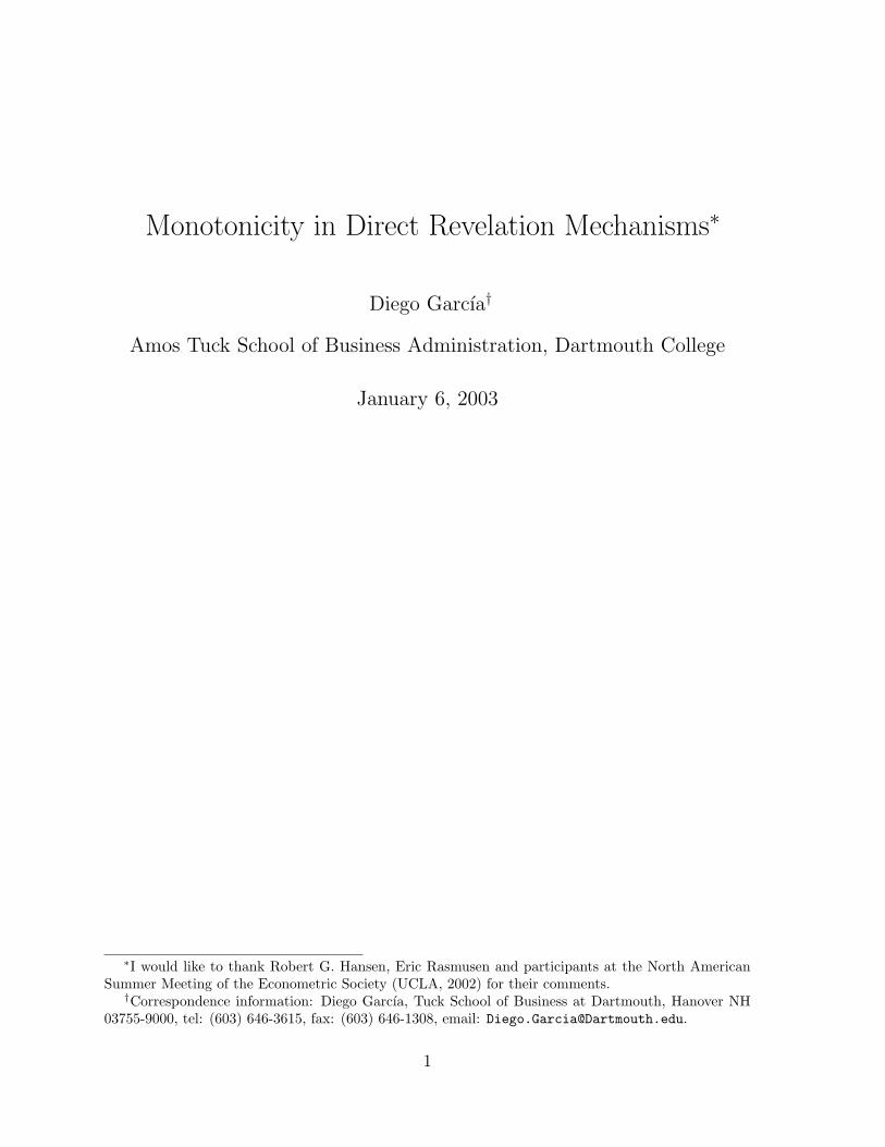
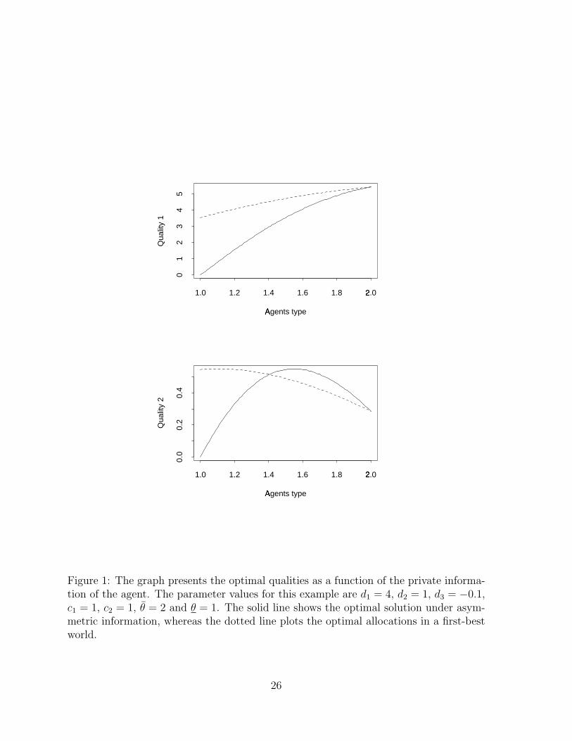
Figure 1 plots the optimal quality schedules for the case where d1 = 4 and d2 = 1
and the two attributes are substitutes with d3 = −0.1. The private information of the
agent is distributed uniformly on [1, 2]. In this particular example for the low range of
private valuations the agent receives increasing allocations of both quality attributes,
whereas for the upper range the quality on the second good is decreasing in θ. �
Example 3. Consider a setting where consumers’ preferences are given by u(x, θ) =
θ(x1 + bx2), where b > 0 is a parameter that represents the relative value of attribute
2 versus attribute 1. Again it is useful to think of xi as the quality along different
dimensions. The cost function for the monopolist takes on the simple quadratic form:
c(x1, x2) = 1/2x21 + 1/2x2
2 + cx1x2. Further assume that θ is distributed as a uniform on
[a, a + 1], so that µ(θ) = 1 + a − θ. The interesting set of parameter values occurs for
small positive values of c, so that the two qualities have a small positive complementarity
in the cost function, and for a > 1 (which guarantees that all agents’ types are served).
The optimal mechanism in the case where one of the qualities is fixed is x1 = 2θ −
1 − a − cx2 if x2 is fixed, or x2 = (2θ − 1)b − a − cx1 in the other case. It is worth
noticing that in both cases dxi/dθ > 0. Moreover, due to the simple structure of the
example this slope is constant. If we allow for the principal to discriminate along both
dimensions, it is straightforward to check that the optimal allocation will be given by14
x2 = (b−c)(2θ−1−a)/(1−c2) and x1 = (1−bc)(2θ−1−a)/(1−c2). It is immediate that
the allocations may not be monotonically increasing: either 1 − cb < 0 or b < c imply
everywhere decreasing allocations.15 Note that even when c is small, if the valuation b
14Note that I am allowing the quality variables to take on any value on R: the simple structure ofthis example could be adjusted to rule out negative values for quality.
15One may wonder whether this result is due to the fact that the monotonicity constraint is beingignored. It is easy to check that (6) will not bind as long as 1 + b2 − 2cb ≥ 0, e.g. for c small. Thereforethis is a robust example of decreasing allocations, i.e. there exists an open set of the parameters forwhich one of the allocations is decreasing in the consumers’ type.
19
for the second quality x2 is large enough this will create an incentive for the monopolist
to design a product line in which the quality increases in the valuable dimension x2, and
decreases in the quality dimension x1. �
Example 4. Consider an agency setting where the agent contributes effort e, and the
principal also takes a productive action a. Final output X is Gaussian, with mean
E [X|s] ≡ m(e, a, θ) = (bee + baa)θ + boe, for some bi ∈ R+, and variance σ2. Incurring
efforts e and a have cost for the agent and the principal of e2/2 and a2/2 respectively.
The principal is risk-neutral and the agent risk-averse, with CARA preferences and risk-
aversion parameter R. The contracts that the principal offers the agent are assumed to
be of the linear form α+βX.16 The principal’s payoff is UP (·) = −α+(1−β)m(·)−a2/2
and the agent’s, in certainty equivalent terms, UA(·) = α + βm(·)− R2β2σ2 − e2/2. Note
that in contrast to the classic moral hazard model (Holmstrom (1979)) here I allow the
principal to affect the output as well. This has a similar flavor to the agency models where
an investment decision is at the discretion of the principal (e.g. Bernardo, Cai, and Luo
(2001), Sung (2001)), and the transfer pricing problem with moral hazard of Besanko and
Sibley (1991). In a second-best world, where the action e is unobservable, but the private
information θ is observable, the optimal contract is given by β = 1/(1+Rσ2/(θbe +bo)2),
with a = θba being the optimal action taken by the principal. The effort exerted by the
agent is e = β(θbe + b0). It is worth noticing that β, a and e are all increasing functions
of the signal θ.
In the case with private information the principal offers a set of menus {α(θ), β(θ), a(θ)}
with the standard participation and incentive compatibility constraints. Note that
now we have an extra constraint for the optimality of the effort choice which imme-
diately implies that e(θ, β) = β(θbe + bo). Using this expression for the optimal ef-
fort choice we can substitute in the agent’s certainty equivalent expression to find that
16In a continuous-time stationary version of this model without adverse selection Holmstrom andMilgrom (1987) show that this is without loss of generality. In Sung (2001) the author shows in asimilar model that the optimality of linear contracts holds even in the presence of private information.
20
u(α, β, a, θ) ≡ UA(α, β, e(θ, β), a) = α + βθbaa + 12β2(bo + θbe)
2 − R2β2σ2. Note that this
expression has the quasi-linear form discussed in this paper, where α plays the role of the
transfer function t and (β, a) are the allocation rule x. Following the previous discussion
the principal’s problem reduces to the maximization of the virtual surplus function
maxβ,a
Φ(β, a) = θbaa+(θbe + bo)2(β−β2/2)− R
2β2σ2− 1
2a2−µ(θ)β[aba +βbe(bo + θbe)]
The last term measures the informational cost: the other terms correspond to the
second-best case in which effort is unobservable but there is no private information.
Some tedious calculations show that the optimal bonus coefficient β and action for the
principal a at an interior solution are given by
β(θ) =(θbe + bo)
2 − µ(θ)θb2a
(θbe + bo)2 + Rσ2 + 2µ(θ)be(θbe + bo)− µ(θ)2b2a
;
a = ba(θ − µ(θ)β(θ)).
Notice that, using the previous notation, uθaβ = ba > 0, and also that ΦFBaβ = 0.
Using Proposition 2 it is immediate that for ba large the optimal allocations may be
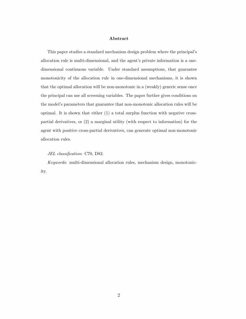
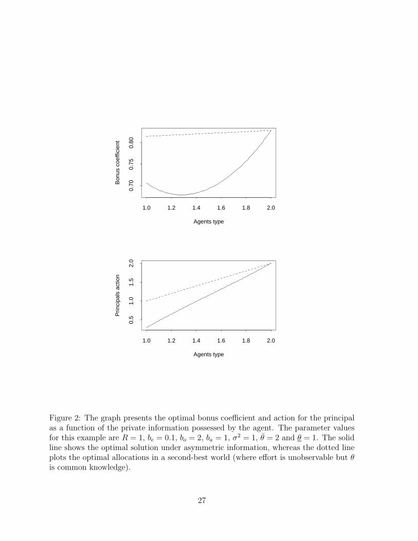
non-monotone.17 Figure 2 plots the optimal bonus coefficient for a set of reasonable
parameter values: bo = 2, ba = 1, be = 0.1, σ2 = 1, θ = 1 and θ = 2. Both e, β and
a are below their respective second-best values (plotted as dotted lines). Moreover, the
bonus coefficient is a non-monotone function of the private information of the agent. The
indirect informational effect discussed after Proposition 2 overcomes the direct informa-
tional effect (i.e. the one that prevails in one-dimensional models) for the parameter
values under consideration.18 �17Second-order conditions need to be checked, otherwise the statement is unconditional.18One can easily check that the sufficient conditions given in Proposition 1 hold in this numerical
example.
21
4 Conclusion
This paper has studied a standard mechanism design problem with quasi-linear pref-
erences in the case where the allocation rule over which parties negotiate is multi-
dimensional, but the agent’s information can be described by a one-dimensional param-
eter. It has been shown that, in contrast to one-dimensional problems, the allocation
rules may be non-monotonic functions of the private information of the agent, even in
models where the incentive compatibility constraints bind locally. The paper also gives a
set of conditions under which this non-monotonicity property of the optimal allocations
is likely to arise. The optimality of non-monotonic allocation rules should bring caution
to reduced-form empirical tests of asymmetric information models. In particular, this
paper points out that qualitative predictions based on one-dimensional models may not
be the appropriate reduced-form tests, since with one single screening variable mono-
tonicity is an immediate implication of these models, whereas in general this may not
be the case.
22
References
Baron, D. P., and R. B. Myerson, 1982, “Regulating a monopolist with unknown costs,”
Econometrica, 50(4), 911–930.
Bernardo, A. E., H. Cai, and J. Luo, 2001, “Capital Budgeting and Compensation with
Asymmetric Information and Moral Hazard,” Journal of Financial Economics, 61(3),
311–344.
Besanko, D., and D. S. Sibley, 1991, “Compensation and Transfer Pricing in a Principal-
Agent Model,” International Economic Review, 32(1), 55–68.
Caillaud, B., R. Guesnerie, P. Rey, and J. Tirole, 1988, “Government intervention in
production and incentives theory: a review of recent contributions,” RAND Journal
of Economics, 219(1), 1–26.
Calzolari, G., 2001, “Incentive Regulation of Multinational Enterprises,” working paper,
GREMAG, Universite des Sciences Sociales de Toulouse.
Fudenberg, D., and J. Tirole, 1991, Game Theory. MIT Press, Cambridge, Mass.
Garcıa, D., 2001, “Retained equity, investment decisions and private information,” work-
ing paper, Amos Tuck School of Business, Dartmouth College.
Guesnerie, R., and J.-J. Laffont, 1984, “A Complete Solution to a Class of Principal-
Agent Problems with an Application to the Control of a Self-Managed Firm,” Journal
of Public Economics, 25, 329–369.
Harris, M., C. Kriebel, and A. Raviv, 1982, “Asymmetric Information, Incentives and
Intrafirm Resource Allocation,” Management Science, 28(6), 604–620.
Holmstrom, B., 1979, “Moral Hazard and Observability,” Bell Journal of Economics,
10(1), 74—91.
23
Holmstrom, B., and P. Milgrom, 1987, “Aggregation and Linearity in the Provision of
Intertemporal Incentives,” Econometrica, 55, 303—328.
Matthews, S., and J. Moore, 1987, “Monopoly Provision of Quality and Warranties:
An Exploration in the Theory of Multidimensional Screening,” Econometrica, 55(2),
441–467.
Mirman, L. J., and D. Sibley, 1980, “Optimal nonlinear prices for multiproduct monop-
olies,” Bell Journal of Economics, 11(2), 659–670.
Mirrlees, J. A., 1971, “An exploration in the theory of optimal income taxation,” Review
of Economic Studies, 38, 175–208.
Mussa, M., and S. Rosen, 1978, “Monopoly and Product Quality,” Journal of Economic
Theory, 18, 301–317.
Myerson, R., 1981, “Optimal Auction Design,” Mathematics of Operations Research,
6(1), 58–73.
Roberts, K., 1979, “Welfare Considerations of Nonlinear Pricing,” Economic Journal,
89, 66–83.
Rochet, J.-C., 1987, “A Necessary and Sufficient Condition for Rationalizability in a
Quasi-Linear Context,” Journal of Mathematical Economics, 16, 191–200.
Rochet, J.-C., and L. A. Stole, 2000, “The Economics of Multidimensional Screening,”
working paper, University of Chicago.
Spence, A. M., 1980, “Multi-Product Quantity-Dependent Prices and Profitability Con-
straints,” Review of Economic Studies, 47, 821–841.
Stole, L. A., 1997, “Lectures on the Theory of Contracts and Organizations,” working
paper, University of Chicago.
24

Sung, J., 2001, “Optimal Contracts under Moral Hazard and Adverse Selection: a
Continuous-Time Approach,” working paper, University of Illinois at Chicago.
van Egteren, H., 1996, “Regulating an externality-generating public utility: A multi-
dimensional screening approach,” European Economic Review, 40, 1773–1797.
25
Agents type�
Qua
lity
1
1.0 1.2 1.4 1.6 1.8 2.0�
01
23
45
Agents type�
Qua
lity
2
1.0 1.2 1.4 1.6 1.8 2.0�
0.0
0.2
0.4
Figure 1: The graph presents the optimal qualities as a function of the private informa-tion of the agent. The parameter values for this example are d1 = 4, d2 = 1, d3 = −0.1,c1 = 1, c2 = 1, θ = 2 and θ = 1. The solid line shows the optimal solution under asym-metric information, whereas the dotted line plots the optimal allocations in a first-bestworld.
26
Agents type
Bon
us c
oeffi
cien
t
1.0 1.2 1.4 1.6 1.8 2.0
0.70
0.75
0.80
Agents type
Prin
cipa
ls a
ctio
n
1.0 1.2 1.4 1.6 1.8 2.0
0.5
1.0
1.5
2.0
Figure 2: The graph presents the optimal bonus coefficient and action for the principalas a function of the private information possessed by the agent. The parameter valuesfor this example are R = 1, be = 0.1, bo = 2, ba = 1, σ2 = 1, θ = 2 and θ = 1. The solidline shows the optimal solution under asymmetric information, whereas the dotted lineplots the optimal allocations in a second-best world (where effort is unobservable but θis common knowledge).
27


![A Revelation Principle for Competing Mechanismspeople.bu.edu/lepstein/files-research/epstein-peters99.pdf · mechanisms [14, 21, 22] restricts sellers to direct mechanisms in which](https://static.cupdf.com/doc/110x72/6023d86221ac662fd8003fbd/a-revelation-principle-for-competing-mechanisms-14-21-22-restricts-sellers-to.jpg)