Frequency functions, monotonicity formulas, and the thin obstacle problem Donatella Danielli - Purdue University IMA - University of Minnesota March 4, 2013 Donatella Danielli - Purdue University The Thin Obstacle Problem IMA - University of Minnesota March 4, 201 / 45

Welcome message from author
This document is posted to help you gain knowledge. Please leave a comment to let me know what you think about it! Share it to your friends and learn new things together.
Transcript

Frequency functions, monotonicity formulas, and thethin obstacle problem
Donatella Danielli - Purdue University
IMA - University of MinnesotaMarch 4, 2013
Donatella Danielli - Purdue University The Thin Obstacle ProblemIMA - University of Minnesota March 4, 2013 1
/ 45

Thank you for the invitation!
Donatella Danielli - Purdue University The Thin Obstacle ProblemIMA - University of Minnesota March 4, 2013 2
/ 45
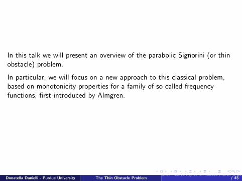
In this talk we will present an overview of the parabolic Signorini (or thinobstacle) problem.
In particular, we will focus on a new approach to this classical problem,based on monotonicity properties for a family of so-called frequencyfunctions, first introduced by Almgren.
Donatella Danielli - Purdue University The Thin Obstacle ProblemIMA - University of Minnesota March 4, 2013 3
/ 45
The Classical Obstacle Problem
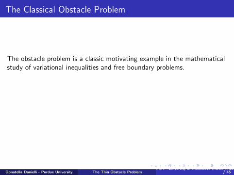
The obstacle problem is a classic motivating example in the mathematicalstudy of variational inequalities and free boundary problems.
The problem consists in finding the equilibrium position of an elasticmembrane whose boundary is held fixed, and which is constrained to lieabove a given obstacle. Applications include the study of fluid filtration inporous media, constrained heating, elasto-plasticity, optimal control, andfinancial mathematics.
Donatella Danielli - Purdue University The Thin Obstacle ProblemIMA - University of Minnesota March 4, 2013 4
/ 45
The Classical Obstacle Problem
The obstacle problem is a classic motivating example in the mathematicalstudy of variational inequalities and free boundary problems.
The problem consists in finding the equilibrium position of an elasticmembrane whose boundary is held fixed, and which is constrained to lieabove a given obstacle. Applications include the study of fluid filtration inporous media, constrained heating, elasto-plasticity, optimal control, andfinancial mathematics.
Donatella Danielli - Purdue University The Thin Obstacle ProblemIMA - University of Minnesota March 4, 2013 4
/ 45
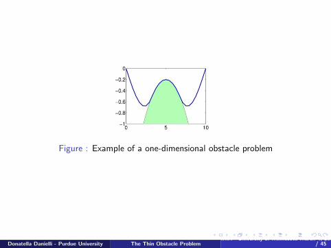
Figure : Example of a one-dimensional obstacle problem
Donatella Danielli - Purdue University The Thin Obstacle ProblemIMA - University of Minnesota March 4, 2013 5
/ 45
Mathematically, the obstacle problem consists of studying the properties ofminimizers of the Dirichlet integral
J(u) =
∫D|∇u|2 dx
in a domain D ⊂ Rn, among all configurations u(x) (representing thevertical displacement of the membrane) with prescribed boundary valuesu|∂D = f (x), and constrained to remain above the obstacle ϕ(x).
The solution breaks down into a region where the solution is equal to theobstacle function, known as the coincidence set, and a region where thesolution is above the obstacle. The interface between the two regions isthe so-called free boundary.
Donatella Danielli - Purdue University The Thin Obstacle ProblemIMA - University of Minnesota March 4, 2013 6
/ 45
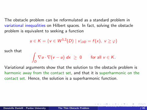
The obstacle problem can be reformulated as a standard problem invariational inequalities on Hilbert spaces. In fact, solving the obstacleproblem is equivalent to seeking a function
u ∈ K = v ∈W 1,2(D) | v |∂D = f (x), v ≥ ϕ
such that ∫D∇u · ∇(v − u) dx ≥ 0 for all v ∈ K .
Variational arguments show that the solution to the obstacle problem isharmonic away from the contact set, and that it is superharmonic on thecontact set. Hence, the solution is a superharmonic function.
Donatella Danielli - Purdue University The Thin Obstacle ProblemIMA - University of Minnesota March 4, 2013 7
/ 45
The study of the classical obstacle problem, initiated in the 60’s with thepioneering works of G. Stampacchia, H. Lewy, J. L. Lions, has led tobeautiful and deep developments in calculus of variations and geometricpartial differential equations. The crowning achievement has been thedevelopment, due to L. Caffarelli, of the theory of free boundaries.
Donatella Danielli - Purdue University The Thin Obstacle ProblemIMA - University of Minnesota March 4, 2013 8
/ 45
Optimal regularity of the solution The solution to the obstacle problemis C 1,1 (i.e. it has bounded second derivatives) when the obstacle itself hassuch regularity. In general, the second derivatives of the solutions arediscontinuous across the free boundary.
The free boundary The free boundary is characterized as a Holdercontinuous surface except at certain singular points, which are eitherisolated or contained on a C 1 manifold.
Donatella Danielli - Purdue University The Thin Obstacle ProblemIMA - University of Minnesota March 4, 2013 9
/ 45
Background: The time-independent thin obstacle problem
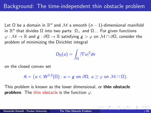
Let Ω be a domain in Rn and M a smooth (n − 1)-dimensional manifoldin Rn that divides Ω into two parts: Ω+ and Ω−. For given functionsϕ :M→ R and g : ∂Ω→ R satisfying g > ϕ on M∩ ∂Ω, consider theproblem of minimizing the Dirichlet integral
DΩ(u) =
∫Ω|∇u|2dx
on the closed convex set
K = u ∈W 1,2(Ω) : u = g on ∂Ω, u ≥ ϕ on M∩ Ω.
This problem is known as the lower dimensional, or thin obstacleproblem. The thin obstacle is the function ϕ.
Donatella Danielli - Purdue University The Thin Obstacle ProblemIMA - University of Minnesota March 4, 2013 10
/ 45
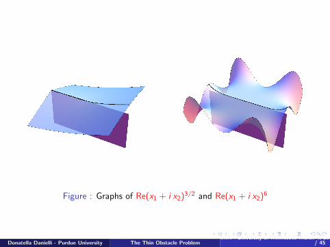
Figure : Graphs of Re(x1 + i x2)3/2 and Re(x1 + i x2)6
Donatella Danielli - Purdue University The Thin Obstacle ProblemIMA - University of Minnesota March 4, 2013 11
/ 45
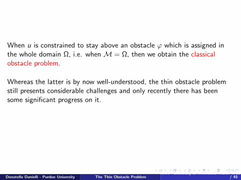
When u is constrained to stay above an obstacle ϕ which is assigned inthe whole domain Ω, i.e. when M = Ω, then we obtain the classicalobstacle problem.
Whereas the latter is by now well-understood, the thin obstacle problemstill presents considerable challenges and only recently there has beensome significant progress on it.
Donatella Danielli - Purdue University The Thin Obstacle ProblemIMA - University of Minnesota March 4, 2013 12
/ 45
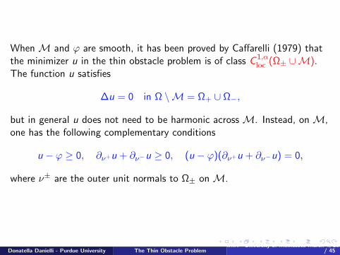
When M and ϕ are smooth, it has been proved by Caffarelli (1979) thatthe minimizer u in the thin obstacle problem is of class C 1,α
loc (Ω± ∪M).The function u satisfies
∆u = 0 in Ω \M = Ω+ ∪ Ω−,
but in general u does not need to be harmonic across M. Instead, on M,one has the following complementary conditions
u − ϕ ≥ 0, ∂ν+u + ∂ν−u ≥ 0, (u − ϕ)(∂ν+u + ∂ν−u) = 0,
where ν± are the outer unit normals to Ω± on M.
Donatella Danielli - Purdue University The Thin Obstacle ProblemIMA - University of Minnesota March 4, 2013 13
/ 45
One of the main goals in the study of this problem is to understand theproperties of the coincidence set
Λ(u) := x ∈M : u = ϕ
and its boundary (in the relative topology of M)
Γ(u) := ∂MΛ(u),
i.e., the free boundary.
Simplifying assumptions:1. Vanishing thin obstacle ϕ.2. The manifold M is a flat portion of the boundary of the relevantdomain: M=Rn−1 × 0. In this case the thin obstacle problem is knownas the Signorini problem.
Donatella Danielli - Purdue University The Thin Obstacle ProblemIMA - University of Minnesota March 4, 2013 14
/ 45
This problem, which arises in linear elasticity, was first proposed bySignorini in 1959. Signorini called it the “problem with ambiguousboundary conditions”. The existence and uniqueness of solutions wasproved by Fichera in 1963. It was Fichera who renamed it as “Signoriniproblem”.
In the original formulation, it consists of finding the elastic equilibriumconfiguration of an anisotropic non-homogeneous elastic body, resting on arigid frictionless surface and subject only to its mass forces.
Donatella Danielli - Purdue University The Thin Obstacle ProblemIMA - University of Minnesota March 4, 2013 15
/ 45

Figure : What will be the equilibrium configuration of an elastic body resting on arigid frictionless plane?
Donatella Danielli - Purdue University The Thin Obstacle ProblemIMA - University of Minnesota March 4, 2013 16
/ 45
Other applications include optimal control of temperature across a surface,in the modeling of semipermeable membranes where some salineconcentration can flow through the membrane only in one direction, andfinancial math (when the random variation of underlying asset changes ina discontinuous fashion, as a Levi process).
Donatella Danielli - Purdue University The Thin Obstacle ProblemIMA - University of Minnesota March 4, 2013 17
/ 45
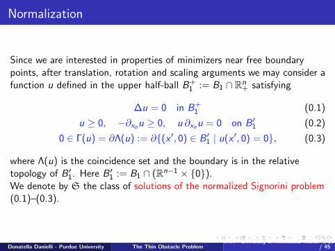
Normalization
Since we are interested in properties of minimizers near free boundarypoints, after translation, rotation and scaling arguments we may consider afunction u defined in the upper half-ball B+
1 := B1 ∩ Rn+ satisfying
∆u = 0 in B+1 (0.1)
u ≥ 0, −∂xnu ≥ 0, u ∂xnu = 0 on B ′1 (0.2)
0 ∈ Γ(u) = ∂Λ(u) := ∂(x ′, 0) ∈ B ′1 | u(x ′, 0) = 0, (0.3)
where Λ(u) is the coincidence set and the boundary is in the relativetopology of B ′1. Here B ′1 := B1 ∩ (Rn−1 × 0).We denote by S the class of solutions of the normalized Signorini problem(0.1)–(0.3).
Donatella Danielli - Purdue University The Thin Obstacle ProblemIMA - University of Minnesota March 4, 2013 18
/ 45
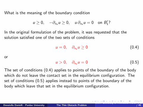
What is the meaning of the boundary condition
u ≥ 0, −∂xnu ≥ 0, u ∂xnu = 0 on B ′1?
In the original formulation of the problem, it was requested that thesolution satisfied one of the two sets of conditions
u = 0, ∂xnu ≥ 0 (0.4)
oru > 0, ∂xnu = 0 (0.5)
The set of conditions (0.4) applies to points of the boundary of the bodywhich do not leave the contact set in the equilibrium configuration. Theset of conditions (0.5) applies instead to points of the boundary of thebody which leave that set in the equilibrium configuration.
Donatella Danielli - Purdue University The Thin Obstacle ProblemIMA - University of Minnesota March 4, 2013 19
/ 45
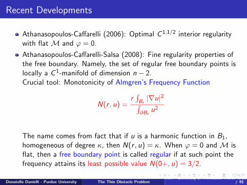
Recent Developments
Athanasopoulos-Caffarelli (2006): Optimal C 1,1/2 interior regularitywith flat M and ϕ = 0.
Athanasopoulos-Caffarelli-Salsa (2008): Fine regularity properties ofthe free boundary. Namely, the set of regular free boundary points islocally a C 1-manifold of dimension n − 2.Crucial tool: Monotonicity of Almgren’s Frequency Function
N(r , u) =r∫Br|∇u|2∫
∂Bru2
The name comes from fact that if u is a harmonic function in B1,homogeneous of degree κ, then N(r , u) = κ. When ϕ = 0 and M isflat, then a free boundary point is called regular if at such point thefrequency attains its least possible value N(0+, u) = 3/2.
Donatella Danielli - Purdue University The Thin Obstacle ProblemIMA - University of Minnesota March 4, 2013 20
/ 45
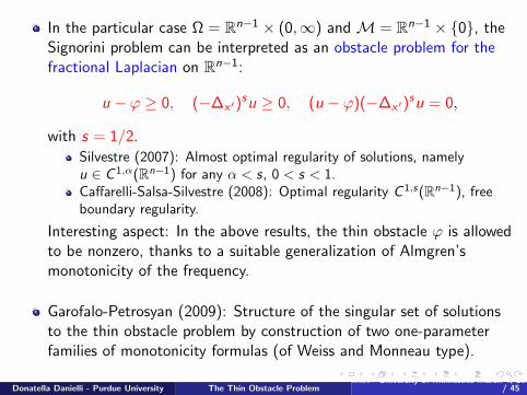
In the particular case Ω = Rn−1 × (0,∞) and M = Rn−1 × 0, theSignorini problem can be interpreted as an obstacle problem for thefractional Laplacian on Rn−1:
u − ϕ ≥ 0, (−∆x ′)su ≥ 0, (u − ϕ)(−∆x ′)
su = 0,
with s = 1/2.
Silvestre (2007): Almost optimal regularity of solutions, namelyu ∈ C 1,α(Rn−1) for any α < s, 0 < s < 1.Caffarelli-Salsa-Silvestre (2008): Optimal regularity C 1,s(Rn−1), freeboundary regularity.
Interesting aspect: In the above results, the thin obstacle ϕ is allowedto be nonzero, thanks to a suitable generalization of Almgren’smonotonicity of the frequency.
Garofalo-Petrosyan (2009): Structure of the singular set of solutionsto the thin obstacle problem by construction of two one-parameterfamilies of monotonicity formulas (of Weiss and Monneau type).
Donatella Danielli - Purdue University The Thin Obstacle ProblemIMA - University of Minnesota March 4, 2013 21
/ 45
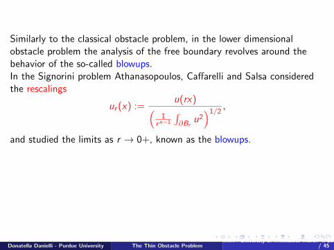
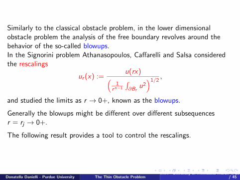
Similarly to the classical obstacle problem, in the lower dimensionalobstacle problem the analysis of the free boundary revolves around thebehavior of the so-called blowups.In the Signorini problem Athanasopoulos, Caffarelli and Salsa consideredthe rescalings
ur (x) :=u(rx)(
1rn−1
∫∂Br
u2)1/2
,
and studied the limits as r → 0+, known as the blowups.
Generally the blowups might be different over different subsequencesr = rj → 0+.
The following result provides a tool to control the rescalings.
Donatella Danielli - Purdue University The Thin Obstacle ProblemIMA - University of Minnesota March 4, 2013 22
/ 45
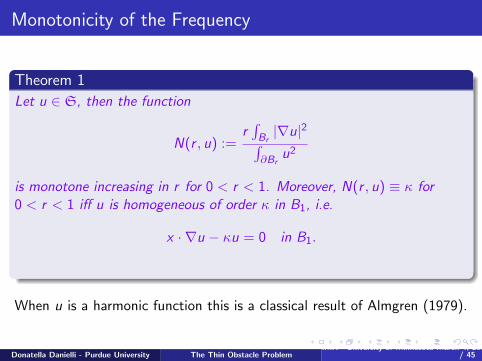
Monotonicity of the Frequency
Theorem 1
Let u ∈ S, then the function
N(r , u) :=r∫Br|∇u|2∫
∂Bru2
is monotone increasing in r for 0 < r < 1. Moreover, N(r , u) ≡ κ for0 < r < 1 iff u is homogeneous of order κ in B1, i.e.
x · ∇u − κu = 0 in B1.
When u is a harmonic function this is a classical result of Almgren (1979).
Donatella Danielli - Purdue University The Thin Obstacle ProblemIMA - University of Minnesota March 4, 2013 23
/ 45
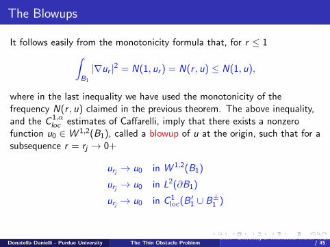
The Blowups
It follows easily from the monotonicity formula that, for r ≤ 1∫B1
|∇ur |2 = N(1, ur ) = N(r , u) ≤ N(1, u),
where in the last inequality we have used the monotonicity of thefrequency N(r , u) claimed in the previous theorem. The above inequality,and the C 1,α
loc estimates of Caffarelli, imply that there exists a nonzerofunction u0 ∈W 1,2(B1), called a blowup of u at the origin, such that for asubsequence r = rj → 0+
urj → u0 in W 1,2(B1)
urj → u0 in L2(∂B1)
urj → u0 in C 1loc(B ′1 ∪ B±1 )
Donatella Danielli - Purdue University The Thin Obstacle ProblemIMA - University of Minnesota March 4, 2013 24
/ 45
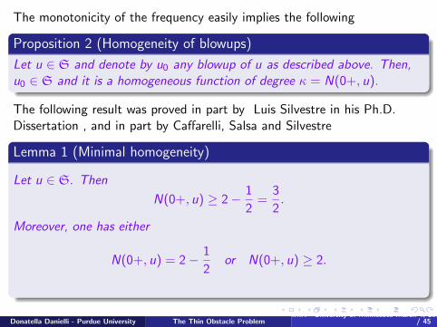
The monotonicity of the frequency easily implies the following
Proposition 2 (Homogeneity of blowups)
Let u ∈ S and denote by u0 any blowup of u as described above. Then,u0 ∈ S and it is a homogeneous function of degree κ = N(0+, u).
The following result was proved in part by Luis Silvestre in his Ph.D.Dissertation , and in part by Caffarelli, Salsa and Silvestre
Lemma 1 (Minimal homogeneity)
Let u ∈ S. Then
N(0+, u) ≥ 2− 1
2=
3
2.
Moreover, one has either
N(0+, u) = 2− 1
2or N(0+, u) ≥ 2.
Donatella Danielli - Purdue University The Thin Obstacle ProblemIMA - University of Minnesota March 4, 2013 25
/ 45
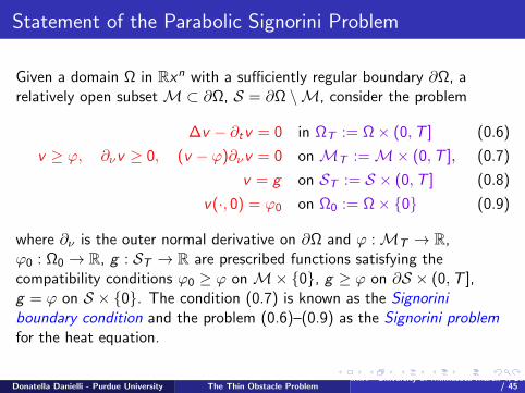
Statement of the Parabolic Signorini Problem
Given a domain Ω in Rxn with a sufficiently regular boundary ∂Ω, arelatively open subset M⊂ ∂Ω, S = ∂Ω \M, consider the problem
∆v − ∂tv = 0 in ΩT := Ω× (0,T ] (0.6)
v ≥ ϕ, ∂νv ≥ 0, (v − ϕ)∂νv = 0 on MT :=M× (0,T ], (0.7)
v = g on ST := S × (0,T ] (0.8)
v(·, 0) = ϕ0 on Ω0 := Ω× 0 (0.9)
where ∂ν is the outer normal derivative on ∂Ω and ϕ :MT → R,ϕ0 : Ω0 → R, g : ST → R are prescribed functions satisfying thecompatibility conditions ϕ0 ≥ ϕ on M×0, g ≥ ϕ on ∂S × (0,T ],g = ϕ on S × 0. The condition (0.7) is known as the Signoriniboundary condition and the problem (0.6)–(0.9) as the Signorini problemfor the heat equation.
Donatella Danielli - Purdue University The Thin Obstacle ProblemIMA - University of Minnesota March 4, 2013 26
/ 45
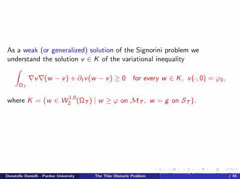
As a weak (or generalized) solution of the Signorini problem weunderstand the solution v ∈ K of the variational inequality∫
ΩT
∇v∇(w − v) + ∂tv(w − v) ≥ 0 for every w ∈ K , v(·, 0) = ϕ0,
where K = w ∈W 1,02 (ΩT ) | w ≥ ϕ on MT , w = g on ST.
Donatella Danielli - Purdue University The Thin Obstacle ProblemIMA - University of Minnesota March 4, 2013 27
/ 45
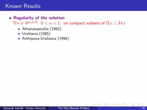
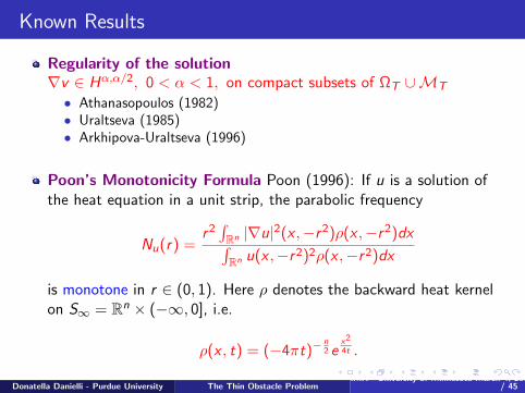
Known Results
Regularity of the solution∇v ∈ Hα,α/2, 0 < α < 1, on compact subsets of ΩT ∪MT
• Athanasopoulos (1982)• Uraltseva (1985)• Arkhipova-Uraltseva (1996)
Poon’s Monotonicity Formula Poon (1996): If u is a solution ofthe heat equation in a unit strip, the parabolic frequency
Nu(r) =r 2∫Rn |∇u|2(x ,−r 2)ρ(x ,−r 2)dx∫Rn u(x ,−r 2)2ρ(x ,−r 2)dx
is monotone in r ∈ (0, 1). Here ρ denotes the backward heat kernelon S∞ = Rn × (−∞, 0], i.e.
ρ(x , t) = (−4πt)−n2 e
x2
4t .
Donatella Danielli - Purdue University The Thin Obstacle ProblemIMA - University of Minnesota March 4, 2013 28
/ 45
Notations
Rn = x = (x1, x2, . . . , xn) : xi ∈ R (Euclidean space)
Rn+ = Rn ∩ xn > 0 (positive halfspace)
Rn− = Rn ∩ xn < 0 (negative halfspace)
Rn−1 ∼ Rn−1 × 0 ⊂ Rn
x ′ = (x1, x2, . . . , xn−1),
x ′′ = (x1, x2, . . . , xn−2)
x = (x ′, xn), x ′ = (x ′′, xn−1)
Donatella Danielli - Purdue University The Thin Obstacle ProblemIMA - University of Minnesota March 4, 2013 29
/ 45
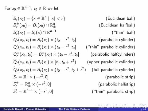
For x0 ∈ Rn−1, t0 ∈ R we let
Br (x0) = x ∈ Rn | |x | < r (Euclidean ball)
B±r (x0) = Br (x0) ∩ Rn± (Euclidean halfball)
B ′r (x0) = Br (x) ∩ Rn−1 (“thin” ball)
Qr (x0, t0) = Br (x0)× (t0 − r 2, t0] (parabolic cylinder)
Q ′r (x0, t0) = B ′r (x0)× (t0 − r 2, t0] (“thin” parabolic cylinder)
Q±r (x0, t0) = B±r (x0)× (t0 − r 2, t0] (parabolic halfcylinders)
Qr (x0, t0) = Br (x0)× [t0, t0 + r 2) (upper parabolic cylinder)
Qr (x0, t0) = Br (x0)× (t0 − r 2, t0 + r 2) (full parabolic cylinder)
Sr = Rn × (−r 2, 0] (parabolic strip)
S±r = Rn± × (−r 2, 0] (parabolic halfstrip)
S ′r = Rn−1 × (−r 2, 0] (“thin” parabolic strip)
Donatella Danielli - Purdue University The Thin Obstacle ProblemIMA - University of Minnesota March 4, 2013 30
/ 45
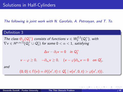
Solutions in Half-Cylinders
The following is joint work with N. Garofalo, A. Petrosyan, and T. To.
Definition 3
The class Sϕ(Q+1 ) consists of functions v ∈W 2,1
2 (Q+1 ), with
∇v ∈ Hα,α/2(Q+1 ∪ Q ′1) for some 0 < α < 1, satisfying
∆v − ∂tv = 0 in Q+1
v − ϕ ≥ 0, −∂xnv ≥ 0, (v − ϕ)∂xnv = 0 on Q ′1,
and(0, 0) ∈ Γ(v) = ∂(x ′, t) ∈ Q ′1 | v(x ′, 0, t) > ϕ(x ′, t).
Donatella Danielli - Purdue University The Thin Obstacle ProblemIMA - University of Minnesota March 4, 2013 31
/ 45
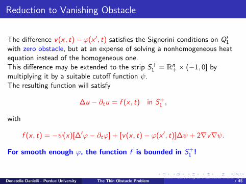
Reduction to Vanishing Obstacle
The difference v(x , t)− ϕ(x ′, t) satisfies the Signorini conditions on Q ′1with zero obstacle, but at an expense of solving a nonhomogeneous heatequation instead of the homogeneous one.This difference may be extended to the strip S+
1 = Rn+ × (−1, 0] by
multiplying it by a suitable cutoff function ψ.The resulting function will satisfy
∆u − ∂tu = f (x , t) in S+1 ,
with
f (x , t) = −ψ(x)[∆′ϕ− ∂tϕ] + [v(x , t)− ϕ(x ′, t)]∆ψ + 2∇v∇ψ.
For smooth enough ϕ, the function f is bounded in S+1 !
Donatella Danielli - Purdue University The Thin Obstacle ProblemIMA - University of Minnesota March 4, 2013 32
/ 45
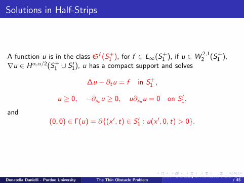
Solutions in Half-Strips
A function u is in the class Sf (S+1 ), for f ∈ L∞(S+
1 ), if u ∈W 2,12 (S+
1 ),∇u ∈ Hα,α/2(S+
1 ∪ S ′1), u has a compact support and solves
∆u − ∂tu = f in S+1 ,
u ≥ 0, −∂xnu ≥ 0, u∂xnu = 0 on S ′1,
and(0, 0) ∈ Γ(u) = ∂(x ′, t) ∈ S ′1 : u(x ′, 0, t) > 0.
Donatella Danielli - Purdue University The Thin Obstacle ProblemIMA - University of Minnesota March 4, 2013 33
/ 45

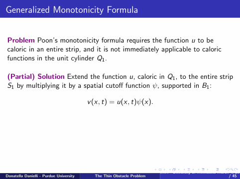
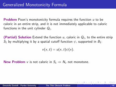
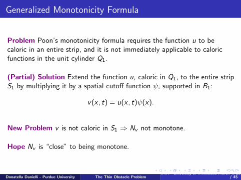
Generalized Monotonicity Formula
Problem Poon’s monotonicity formula requires the function u to becaloric in an entire strip, and it is not immediately applicable to caloricfunctions in the unit cylinder Q1.
(Partial) Solution Extend the function u, caloric in Q1, to the entire stripS1 by multiplying it by a spatial cutoff function ψ, supported in B1:
v(x , t) = u(x , t)ψ(x).
New Problem v is not caloric in S1 ⇒ Nv not monotone.
Hope Nv is “close” to being monotone.
Donatella Danielli - Purdue University The Thin Obstacle ProblemIMA - University of Minnesota March 4, 2013 34
/ 45
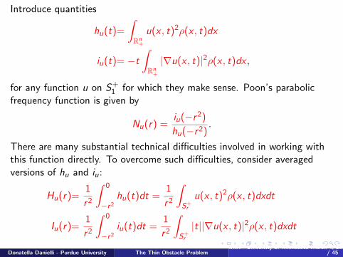
Introduce quantities
hu(t)=
∫Rn
+
u(x , t)2ρ(x , t)dx
iu(t)= −t
∫Rn
+
|∇u(x , t)|2ρ(x , t)dx ,
for any function u on S+1 for which they make sense. Poon’s parabolic
frequency function is given by
Nu(r) =iu(−r 2)
hu(−r 2).
There are many substantial technical difficulties involved in working withthis function directly. To overcome such difficulties, consider averagedversions of hu and iu:
Hu(r)=1
r 2
∫ 0
−r2
hu(t)dt =1
r 2
∫S+r
u(x , t)2ρ(x , t)dxdt
Iu(r)=1
r 2
∫ 0
−r2
iu(t)dt =1
r 2
∫S+r
|t||∇u(x , t)|2ρ(x , t)dxdt
Donatella Danielli - Purdue University The Thin Obstacle ProblemIMA - University of Minnesota March 4, 2013 35
/ 45
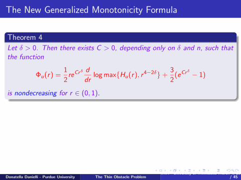
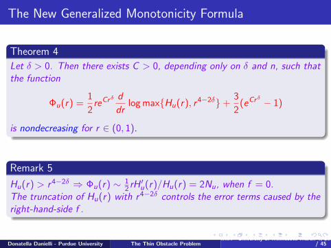
The New Generalized Monotonicity Formula
Theorem 4
Let δ > 0. Then there exists C > 0, depending only on δ and n, such thatthe function
Φu(r) =1
2reCr
δ d
drlog maxHu(r), r 4−2δ+
3
2(eCr
δ − 1)
is nondecreasing for r ∈ (0, 1).
Remark 5
Hu(r) > r 4−2δ ⇒ Φu(r) ∼ 12 rH ′u(r)/Hu(r) = 2Nu, when f = 0.
The truncation of Hu(r) with r 4−2δ controls the error terms caused by theright-hand-side f .
Donatella Danielli - Purdue University The Thin Obstacle ProblemIMA - University of Minnesota March 4, 2013 36
/ 45
With the previous theorem in hands, we can study the existence and thehomogeneity properties of the blow-up’s.Since the function
Φu(r) =1
2reCr
δ d
drlog maxHu(r), r 4−2δ+
3
2(eCr
δ − 1)
is nondecreasing for r ∈ (0, 1), the limit
κ := Φu(0+) = limr→0+
Φu(r)
exists.
Donatella Danielli - Purdue University The Thin Obstacle ProblemIMA - University of Minnesota March 4, 2013 37
/ 45
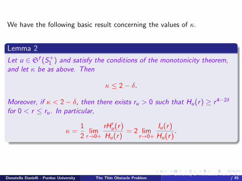
We have the following basic result concerning the values of κ.
Lemma 2
Let u ∈ Sf (S+1 ) and satisfy the conditions of the monotonicity theorem,
and let κ be as above. Then
κ ≤ 2− δ.
Moreover, if κ < 2− δ, then there exists ru > 0 such that Hu(r) ≥ r 4−2δ
for 0 < r ≤ ru. In particular,
κ =1
2lim
r→0+
rH ′u(r)
Hu(r)= 2 lim
r→0+
Iu(r)
Hu(r).
Donatella Danielli - Purdue University The Thin Obstacle ProblemIMA - University of Minnesota March 4, 2013 38
/ 45
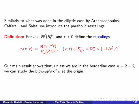
Similarly to what was done in the elliptic case by Athanasopoulos,Caffarelli and Salsa, we introduce the parabolic rescalings.
Definition: For u ∈ Sf (S+1 ) and r > 0 define the rescalings
ur (x , t) :=u(rx , r 2t)
Hu(r)1/2, (x , t) ∈ S+
1/r = Rn+ × (−1/r 2, 0].
Our main result shows that, unless we are in the borderline case κ = 2− δ,we can study the blow-up’s of u at the origin.
Donatella Danielli - Purdue University The Thin Obstacle ProblemIMA - University of Minnesota March 4, 2013 39
/ 45
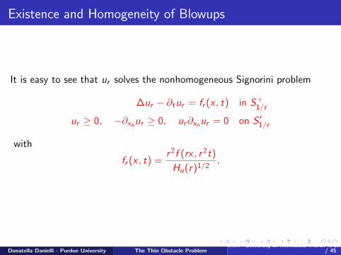
Existence and Homogeneity of Blowups
It is easy to see that ur solves the nonhomogeneous Signorini problem
∆ur − ∂tur = fr (x , t) in S+1/r
ur ≥ 0, −∂xnur ≥ 0, ur∂xnur = 0 on S ′1/r
with
fr (x , t) =r 2f (rx , r 2t)
Hu(r)1/2.
Donatella Danielli - Purdue University The Thin Obstacle ProblemIMA - University of Minnesota March 4, 2013 40
/ 45
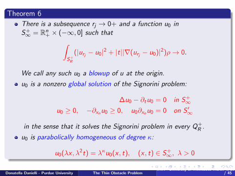
Theorem 6
There is a subsequence rj → 0+ and a function u0 inS+∞ = Rn
+ × (−∞, 0] such that∫S+R
(|urj − u0|2 + |t||∇(urj − u0)|2)ρ→ 0.
We call any such u0 a blowup of u at the origin.
u0 is a nonzero global solution of the Signorini problem:
∆u0 − ∂tu0 = 0 in S+∞
u0 ≥ 0, −∂xnu0 ≥ 0, u0∂xnu0 = 0 on S ′∞
in the sense that it solves the Signorini problem in every Q+R .
u0 is parabolically homogeneous of degree κ:
u0(λx , λ2t) = λκu0(x , t), (x , t) ∈ S+∞, λ > 0
Donatella Danielli - Purdue University The Thin Obstacle ProblemIMA - University of Minnesota March 4, 2013 41
/ 45
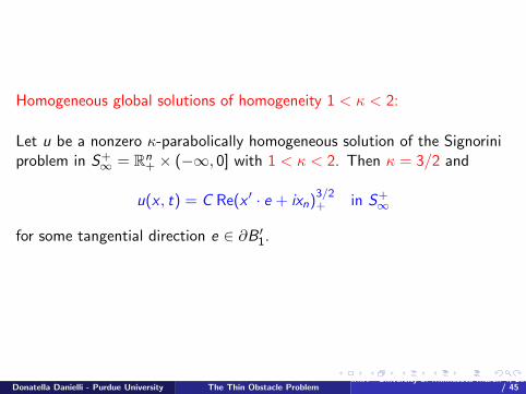
Homogeneous global solutions of homogeneity 1 < κ < 2:
Let u be a nonzero κ-parabolically homogeneous solution of the Signoriniproblem in S+
∞ = Rn+ × (−∞, 0] with 1 < κ < 2. Then κ = 3/2 and
u(x , t) = C Re(x ′ · e + ixn)3/2+ in S+
∞
for some tangential direction e ∈ ∂B ′1.
Donatella Danielli - Purdue University The Thin Obstacle ProblemIMA - University of Minnesota March 4, 2013 42
/ 45
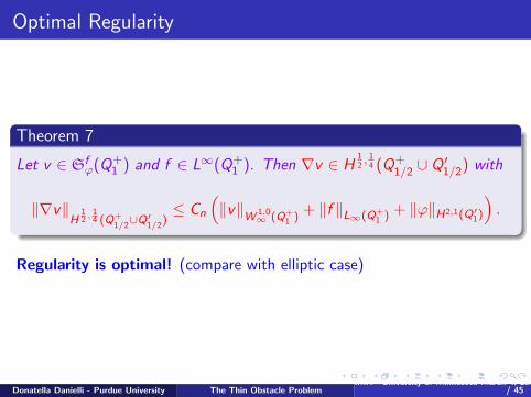
Optimal Regularity
Theorem 7
Let v ∈ Sfϕ(Q+
1 ) and f ∈ L∞(Q+1 ). Then ∇v ∈ H
12, 1
4 (Q+1/2 ∪ Q ′1/2) with
‖∇v‖H
12 ,
14 (Q+
1/2∪Q′
1/2)≤ Cn
(‖v‖
W 1,0∞ (Q+
1 )+ ‖f ‖L∞(Q+
1 ) + ‖ϕ‖H2,1(Q′1)
).
Regularity is optimal! (compare with elliptic case)
Donatella Danielli - Purdue University The Thin Obstacle ProblemIMA - University of Minnesota March 4, 2013 43
/ 45
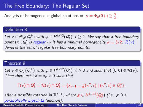
The Free Boundary: The Regular Set
Analysis of homogeneous global solutions ⇒ κ = Φu(0+) ≥ 32 .
Definition 8
Let v ∈ Sϕ(Q+1 ) with ϕ ∈ H`,`/2(Q ′1), ` ≥ 2. We say that a free boundary
point (x0, t0) is regular ⇔ it has a minimal homogeneity κ = 3/2. R(v)denotes the set of regular free boundary points.
Theorem 9
Let v ∈ Sϕ(Q+1 ) with ϕ ∈ H`,`/2(Q ′1), ` ≥ 3 and such that (0, 0) ∈ R(v).
Then there exist δ = δv > 0 such that
Γ(v) ∩ Q ′δ = R(v) ∩ Q ′δ = xn−1 = g(x ′′, t) | (x ′′, t) ∈ Q ′′δ .
after a possible rotation in Rn−1, where g ∈ H1,1/2(Q ′′δ ) (i.e., g is aparabolically Lipschitz function).
Donatella Danielli - Purdue University The Thin Obstacle ProblemIMA - University of Minnesota March 4, 2013 44
/ 45
Thank you for your attention!
Donatella Danielli - Purdue University The Thin Obstacle ProblemIMA - University of Minnesota March 4, 2013 45
/ 45
Related Documents