Inference of monotonicity constraints in datalog programs

Annals of Mathematics and Artificial Intelligence 26 (1999) 29–57 29

Inference of monotonicity constraints in Datalogprograms ∗

Alexander Brodsky a and Yehoshua Sagiv b

a Department of Information and Software Engineering, George Mason University, Fairfax,VA 22030, USA

E-mail: [email protected] Department of Computer Science, Hebrew University, Givat Ram 91904, Jerusalem, Israel

E-mail: [email protected]

Datalog (i.e., function-free logic) programs with monotonicity constraints on extensionalpredicates are considered. A monotonicity constraint states that one argument of a predicateor a constant is always less than another argument or a constant, according to some strictpartial order. Relations of an extensional database are required to satisfy the monotonicityconstraints imposed on their predicates. More specifically, a strict partial order is defined onthe domain (i.e., set of constants) of the database, and every tuple of each relation satisfiesthe monotonicity constraints imposed on its predicate. This paper focuses on the problem ofentailment of monotonicity constraints in the intensional database from monotonicity con-straints in the extensional database. The entailment problem is proven to be decidable, basedon a suggested algorithm for computing sound and complete disjunctions of monotonicityand equality constraints that hold in the intentional database. It is also shown that the entail-ment of monotonicity constraints in programs is a complete problem for exponential time.For linear programs, this problem is complete for polynomial space.

1. Introduction

1.1. Monotonicity constraints, termination and safety

Monotonicity constraints (mcs) state that one argument of a predicate or a constantis always less (or greater) than another argument or a constant, according to some strictpartial order. Typical mcs in logic programs can be based on lengths of terms, or on theknowledge that certain relations are acyclic, e.g., the relation for the parent predicate.Mcs are used to determine termination of top-down evaluation algorithms [1,7], andsafety of programs, i.e., whether programs produce finite relations [5,6] (issues ofsafety also involve finiteness constraints [4]).

Ullman and Van Gelder [7] deal directly with logic programs and constraintsthat are based on sizes of lists, and show how to generate (for a special class of logic

∗ This research was supported in part by grant 85-00082 from the United States–Israel Binational ScienceFoundation (BSF), Jerusalem, Israel, by the NSF grant IRI-9409770 and by the Office of Naval Researchunder the prime grant No. N00014-94-1-1153.

J.C. Baltzer AG, Science Publishers

30 A. Brodsky, Y. Sagiv / Monotonicity constraints in Datalog programs

programs) a set of inequalities whose satisfaction is sufficient for top-down termination.Other papers (e.g., [1,6]) use Datalog (i.e., function-free) programs with relations thatmay be infinite, monotonicity constraints, and finiteness constraints as an abstractionof logic programs. Using this abstraction makes it possible, at least in some cases, toobtain precise characterizations of termination and safety problems (e.g., [1]), whilesimilar problems for general logic programs are undecidable.

1.2. Contributions

We also adopt the Datalog abstraction and address the problem of entailmentof the mcs that hold in intensional predicates from the mcs that hold in extensionalpredicates. In order to solve the entailment problem for mcs, we also consider othertypes of constraints: equality constraints (ecs) and disjunctive constraints (dcs), wherethe latter are just disjunctions of sets (i.e., conjunctions) of mcs and ecs. Mcs andecs will be collectively called atomic constraints (acs). We show that the entailmentproblem for acs and dcs is decidable and develop inference algorithms as follows.

First, we study the entailment problem in relations, i.e., given a set of acs for apredicate, whether another ac must also hold for that predicate. We develop a soundand complete aximatization that allows to compute effectively the set of all entailedacs.

Second, we study the entailment problem for non-recursive Datalog rules, i.e.,given a set of acs for each literal in the body of a rule, whether another ac musthold (in the result computed non-recursively) for the head of the rule. We provide aneffective algorithm that computes, for the head predicate, a set of acs which is sound(i.e., only contains acs that are indeed entailed) and complete (i.e., contains all acs thatare entailed).

Third, we use the entailment algorithms for relations and rules for the entailmentproblem of dcs in Datalog programs. To prove the decidability we devise an effectivealgorithm, that, given a dc for each extensional predicate, finds, for each intentionalpredicate, a dc Q, which is sound (i.e., Q is indeed entailed in the program from theinput dcs) and complete (i.e., Q entails every dc that is entailed in the program). Thus,once Q is computed for an intentional predicate s, a dc G is entailed in the programfor s if and only if it is entailed from Q.

Fourth, we provide complexity results as follows. To check entailment of dcsin a program using our algorithm takes exponential time. If, however, the arity ofpredicates, the number of constants (used in the program and the input dcs), and thenumber of subgoals in each rule are bounded, then the algorithm takes only polynomialtime. We aslo show that the exponential-time upper bound is tight when the arity isunbounded. More specifically, we show that the entailment problem for mcs and theemptiness problem for mcs are complete for exponential time. For linear programs,these problems are complete for polynomial space.

One immediate application of our results is an improvement of [1]. The testof termination described in [1] uses only mcs that hold in extensional predicates. By

A. Brodsky, Y. Sagiv / Monotonicity constraints in Datalog programs 31

inferring mcs that hold in intensional predicates, it is possible to determine terminationby extending the test described in [1] in more cases, and, in general, show that theproblem of top-down termination in presence of mcs is decidable [3].

Our result is also useful in conjunction with that of [5], since their algorithm fordetermining safety uses mcs, but they leave open the entailment problem of mcs.

1.3. Organization of paper

After the introduction in this section, section 2 provides basic definitions. Entail-ment of acs in relations is considered in section 3 and non-recursive entailment in rulesin section 4. Section 5 studies entailment of dcs in Datalog programs. For the sakeof simplicity in exposition, mcs and ecs, as well as rules considered in sections 3–5only involve arguments of predicates, but not constants. Section 6 deals with extend-ing both constraints and programs with constants, and section 7 considers the case ofpartial orders that are linear. Finally, section 8 concludes with the complexity results.An extended abstract of this paper has appeared in [2].

2. Constraints and strict partial orders

A Datalog program consists of function-free Horn-clause rules, i.e., rules of theform

r: q(~Y)

:− p1(~X1), . . . , pn

(~Xn

),

where ~Y and ~X1, . . . , ~Xn are tuples of variables, and q and p1, . . . , pn are predicatesymbols that are not necessarily distinct.

We assume that each variable appearing in the head of a rule must also appearin the body. The extensional predicates are those appearing only in bodies of rules,and the intensional predicates are those appearing in heads of rules. The extensionalpredicates are given initial relations, called the extensional database (EDB), and therules define the intensional database (IDB). Relations may be either finite or infinite.All our results, however, remain the same even if relations are restricted to be finite,because the EDB’s we construct in proofs are always finite.

Let p be a predicate of arity n. We refer to the argument positions (or columns)of p using the integers 1, . . . ,n. The relation for predicate p is denoted as rel(p). If tis a tuple of rel(p) and i is an argument position of p, then t[i] denotes the value of tin column i. Note that t[i] is a constant drawn from some infinite domain.

Generally, constraints of several types may be imposed on the EDB. In this paper,we only consider monotonicity constraints (mcs) [1], and equality constraints (ecs),


which will be collectively referred to as atomic constraints (acs). An mc is a statementof the form1

p: i ≺mc j,

where p is a predicate name and i and j are columns (i.e., argument positions) of p.Intuitively, the above mc means that in each tuple of the relation for p, the value incolumn i is less than the value in column j, according to some strict partial order.

An ec is a statement of the form

p: i =ec j,

where p is a predicate name and i and j are columns of p. Intuitively, the above ecmeans that columns i and j are equal in every tuple of the relation for p.

Formally, we assume that all relations (and all their columns) have the same(infinite) domain D, and there is some strict partial order ≺ defined on D, such that≺ is

(1) transitive, i.e., for all a, b and c in D, a ≺ b and b ≺ c imply a ≺ c, and

(2) irreflexive, i.e., for all a in D, a 6≺ a.

We also assume that ≺ is well-founded, i.e., there does not exist an infinitely decreasingchain a1 � a2 � a3 � · · · . Note, that the properties of transitivity and irreflexivityimply the property of asymmetry, i.e., for all a and b in D, a ≺ b implies b 6≺ a.Therefore, strict partial orders are also asymmetric.

The definitions of satisfaction and consistency of constraints are defined in theusual way as follows:

Definition 1. We say that a relation rel(p) (for predicate p) satisfies an mc p: i ≺mc jwith respect to a strict partial order ≺ if for every tuple t in rel(p), t[i] ≺ t[j]. Wesay that rel(p) satisfies an ec p: i =ec j if for every tuple t in rel(p), t[i] = t[j]. Weshall use the notation rel(p) |=≺ γ, where γ is an ac, to denote that rel(p) satisfies γwith respect to ≺.

We say that rel(p) satisfies a set C of acs with respect to ≺, denoted as rel(p) |=≺C, if rel(p) |=≺ γ for every ac γ in C.

We say that a set C of acs for predicate p is consistent (or satisfiable) if thereexists rel(p) and a strict partial order ≺ on the domain, such that rel(p) |=≺ C.

It should be emphasized that the domain of the database is fixed, although it canbe arbitrarily chosen as long as it is infinite. In other words, the domain does notdepend on the current EDB. The strict partial order defined on the domain, however,is not necessarily fixed. It could be fixed if it depends, for example, on list size (asin [7]). But it could also vary with the EDB if it is based on an EDB relation which

1 We use the symbol ≺mc (rather than ≺) to emphasize that this is a monotonicity constraint and not aspecific strict partial order.


is known to be acyclic (e.g., the relation for the parent predicate). We next considerthe entailment problem in relations.

3. Inference of constraints in relations

Let C and C′ be sets of acs for a predicate p, and γ be an ac for p.

Definition 2. We say that C entails γ, denoted as C |= γ, if for all rel(p) and forall strict partial orders ≺ defined on the domain (of the EDB), rel(p) |=≺ C impliesrel(p) |=≺ γ. Similarly, we say that C entails C′, denoted as C |= C′, if C |= γ forevery γ in C′.

The definition of the entailment is universally quantified not just over all relationsfor p, but also over all strict partial orders that can be defined on the domain, becausein practice a strict partial order may depend on a particular database being considered.For example, a strict partial order may be the one defined by a relation for the predicateparent.

We next present the following axiom and inference rules for acs which will beused for finding constraints that are entailed.

The axiom and inference rules:

` p: i =ec i

p: i ≺mc j, p: j ≺mc k ` p: i ≺mc k

p: i ≺mc j, p: j =ec k ` p: i ≺mc k

p: i =ec j, p: j ≺mc k ` p: i ≺mc k

p: i =ec j, p: j =ec k ` p: i =ec k

p: i =ec j ` p: j =ec i

p: i ≺mc i` p: j ≺mc k, p: j =ec k

The axiom in the first line specifies the ecs that are always satisfied. All theinference rules, except for the last one, are based on the transitivity of strict partialorders and equality, and the symmetry of equality. The last inference rule is used,as we shall see, for completeness, and is based on the fact that the left hand side isinconsistent.

Definition 3. We say that an ac γ can be inferred from a set C of acs, denoted asC ` γ, if γ can be derived from C by means of applying the inference rules and theaxiom.


Of course, we would like to show that the inference rules and the axiom arecorrect in the sense that C implies γ if and only if C infers γ. Then, the question ofimplication can be answered by means of applying the inference rules, i.e., an effectiveprocedure. The notion of correctness is captured here, as usual in a logical setting, bythe concepts of soundness and completeness defined precisely as follows.

Definition 4. We say that the axiom and the inference rules are sound if for every setC of acs and an ac γ, inference of γ from C implies its entailment, i.e.,

C ` γ ⇒ C |= γ.

They are complete if for every C and γ, entailment of γ from C implies its inference,i.e.,

C |= γ ⇒ C ` γ.

We are ready to state correctness of the axiom and inference rules in the followingsimple theorem:

Theorem 3.1.

1. The axiom and inference rules are sound and complete, i.e., for every set C of acsand an ac γ for a predicate p,

C ` γ ⇔ C |= γ.

2. A set C of acs for a predicate p is inconsistent if and only if there exists i such thatp: i ≺mc i is inferred from C, i.e., C ` p: i ≺mc i.

3. If C is consistent, then there exist a tuple t and a strict partial order ≺, such that tsatisfies exactly all acs inferred from C, i.e.,

t |=≺ γ ⇔ C ` γ.

Proof. We prove the theorem’s claims in the following order: Soundness in part 1 isproved first, then part 2, followed by part 3, and, finally, completeness in part 1.

Part 1, soundness. The proof is straightforward by induction on the length of aninference. Clearly, for every i, the axiom is satisfied by every rel(p). The soundnessof each of the inference rules, except for the last one, follows from the transitivity ofstrict partial orders and equality, and the symmetry of equality. The soundness of thelast rule is due to the fact that no rel(p) satisfies an mc of the form p: i ≺mc i, andthus, vacuously, every ac on p is entailed by p: i ≺mc i.

Part 2, IF. If for some i, C ` p: i ≺mc i, then by soundness, C |= p: i ≺mc i. Byirreflexivity of strict partial orders, there do not exist rel(p) and a strict partial order≺, such that rel(p) |=≺ p: i ≺mc i, and therefore, there do not exist rel(p) and ≺, suchthat rel(p) |=≺ C. Thus, C is inconsistent.

Part 2, ONLY IF. We will use the following claim.


Claim 3.1. If for all i, C 0 p: i ≺mc i, then there exist a tuple t and a strict partialorder ≺, such that t satisfies exactly all acs that are inferred from C, i.e.,

t |=≺ γ ⇔ C ` γ.

To prove the claim, suppose that for all i, C 0 p: i ≺mc i. We construct t and ≺as follows. First, we define an equivalence relation ≡ on argument positions of p by

i ≡ j ⇔ C ` p: i =ec j.

Indeed, ≡ is an equivalence relation, since the axiom implies reflexivity, and the fourthand fifth inference rules imply transitivity and symmetry of ≡. Next, we associate adistinct constant c with each equivalence class of ≡. The tuple t is then constructedby taking t[i] = c, where c is the constant assigned to the equivalence class of i.

The strict partial order ≺ is defined by

t[i] ≺ t[j]⇔ C ` p: i ≺mc j.

Indeed, ≺ is a strict partial order, since transitivity follows from the first inferencerule, and irreflexivity follows from the fact that for all i, C 0 p: i ≺mc i. The property

t |=≺ γ ⇔ C ` γ

holds by the construction of t and ≺. This completes the proof of claim 3.1.The ONLY-IF direction of part 2 is now straightforward. If for all i, C 0 p: i ≺mc

i, then claim 3.1 shows that C is consistent.Part 3. Suppose that C is consistent. By part 2 of the theorem (which has been

proved), for all i, C 0 p: i ≺mc i. Thus, part 3 follows directly from claim 3.1.Part 1, Completeness. Suppose C |= γ. We consider two cases, based on whether

C is consistent or not. If C is inconsistent, then part 2 implies that there is an i, suchthat C ` p: i ≺mc i. Thus, by the last inference rule, every ac is inferred from C; inparticular, C ` γ.

If C is consistent, then, by part 3, there are t and ≺, such that

t |=≺ γ ⇔ C ` γ.

Suppose, by way of contradiction, that C 0 γ. Then, t 6|=≺ γ, while t |=≺ C, andhence, t is a counterexample to the fact that C |= γ. A contradiction. �

4. Nonrecursive inference in rules

In this section, we consider the following Datalog rule (denoted as r):

r: q(~Y)

:− p1(~X1), . . . , pn

(~Xn

).


Note that ~Y and ~X1, . . . , ~Xn are tuples of variables,2 predicates p1, . . . , pn are notnecessarily distinct, and predicate q may be one of them. In this section, we viewrule r as a nonrecursive rule (even if predicate q appears in the body). We assume thateach pi has a corresponding relation, denoted as rel(pi), and rule r is applied to theserelations in order to generate new tuples for q. The new tuples are not added to theexisting relation for q (thus, the application is nonrecursive). The relation consistingof the new tuples is called the nonrecursive result of rule r and is denoted as new(q)(rel(q) denotes the relation for q before the rule is applied and is relevant only if qappears in the body).

Each pi has a corresponding set Ci of acs, and rel(pi) satisfies Ci (1 6 i 6 n).The problem we consider in this section is that of determining the acs that hold innew(q), and is defined precisely as follows.

Definition 5. We say that C1, . . . , Cn entail nonrecursively an ac γ in (the result of)rule r, denoted as C1, . . . , Cn |=r γ, if for all strict partial orders ≺ and for all relationsrel(p1), . . . , rel(pn), the following holds:

rel(p1) |=≺ C1, . . . , rel(pn) |=≺ Cn ⇒ new(q) |=≺ γ.

Similarly to entailment in relations, we are interested in finding the set B of allentailed acs. This notion is captured by the properties of soundness and completeness,defined as follows.

Definition 6. We say that B is a sound set of entailed acs with respect to a rule r andC1, . . . , Cn if for every ac γ,

γ ∈ B ⇒ C1, . . . , Cn |=r γ.

Similarly, we say that B is complete if for every ac γ,

C1, . . . , Cn |=r γ ⇒ γ ∈ B.

The following algorithm finds the sound and complete set B. Clearly, if B canbe effectively computed, then the problem of nonrecursive entailment in rule r of anac γ from C1, . . . , Cn is decidable.

Algorithm 1Input: Rule r and C1, . . . , Cn.Output: The set B of acs that is sound and complete with respect to r and C1, . . . , Cn.

Step 1. Variable replacement according to ecs.If variables U and V appear in columns i and j, respectively, of pk( ~Xk) (1 6 k 6 n)and the ec pk : i =ec j is in Ck, then all occurrences of U (in the head and body)are replaced with V . We call the resulting rule r′.

2 Until section 6, we will assume that rules (and constraints) do not have constants.


Step 2. Construct a directed graph G as follows.G has a node for each variable of r′. There is an arc from (the node for) U to V ifU and V appear in columns i and j, respectively, of pk( ~Xk) (1 6 k 6 n) and themc pk : i ≺mc j is in Ck.

Step 3. Construct the output set B for the predicate q as follows.If G has a cycle, then B is defined to contain all acs on q, and is denoted byALL-ACS.Otherwise (i.e., G does not have a cycle), B contains the following acs:

• The ec q : i =ec j is in B if columns i and j of q(~Y ) (the head of rule r) havethe same variable.

• The mc q : i ≺mc j is in B if columns i and j of q(~Y ) have variables U and V ,respectively, and there is a directed path (in G) from U to V .

End (of algorithm)

Example 4.1. Consider the rule

q(X,Y ) :− e(X,Z), q(Z,Y ).

Suppose that q has the ec q : 1 =ec 2 and e has the mc e: 1 ≺mc 2. At first, we replaceall occurrences of Z with Y , due to the ec q : 1 =ec 2, and obtain the rule

q(X,Y ) :− e(X,Y ), q(Y ,Y ).

Now, we construct the graph G consisting of nodes for X and Y and an arc from Xto Y (due to the mc e: 1 ≺mc 2). Since there is a path from X to Y , B contains themc q : 1 ≺mc 2. Obviously, this is the only (nontrivial) ac in B.

The following proposition is an immediate consequence of the construction of Gand B in algorithm 1.

Proposition 4.1.

(i) B is consistent if and only if G has no cycles,

(ii) The set B is closed under the inference rules of section 3,

γ ∈ B ⇔ B ` γ (⇔ B |= γ).

Our goal is to show that B is a sound and complete set of acs for tuples generatedby nonrecursive applications of r. Essentially, we do it by first defining a strict partialorder ≺ and a tuple t, such that t satisfies exactly the constraints of B with respectto ≺, and then showing that t can be generated from some tuples s1, . . . , sn thatare substituted in the body of r. Tuples s1, . . . , sn may have new constants that donot appear in t, and therefore, it is necessary to extend the definition of ≺ to thenew constants (in order to guarantee that s1, . . . , sn satisfy the constraints of their


predicates). A crucial property of the construction is that although ≺ is extended, itremains the same over the constants of t.

In order to show soundness and completeness, we will now develop the necessarymachinery of lemmas. These lemmas will also be used in later sections, and aremore general than what is needed just for showing soundness and completeness ofnonrecursive entailment.

The first lemma is a general result about combining a (possibly infinite) numberof domains and the strict partial orders defined on those domains, such that on oneparticular domain, D0, the definition of the strict partial order does not change.

Lemma 4.1. Suppose that D0 is a domain with a strict partial order ≺0, and considera (possibly infinite) sequence of domains D1, . . . ,Dn, . . . with strict partial orders≺1, . . . ,≺n, . . . , respectively, such that

(1) for all i > 1 and for all a and b in D0,

a ≺i b ⇒ a ≺0 b

(i.e., the strict partial order ≺i is subsumed by ≺0 on D0), and

(2) if i, j > 1 and i 6= j, then Di ∩Dj ⊆ D0.

Let D =⋃i>0 Di. Let ≺ denote the transitive closure of the union of ≺0,≺1, . . . ,

≺n, . . . . Then ≺ is a strict partial order on D that coincides with ≺0 on D0, that is,for all constants a and b in D0,

a ≺0 b⇔ a ≺ b.

Proof. It is convenient to construct a directed graph consisting of the constants of Dand having arcs as follows. If there is a j > 0, such that a ≺j b, then there is an arc,called a ≺j-arc, from a to b. Note that by the assumptions of the lemma, if there ismore than one arc from a to b, then one of those arcs must be a ≺0-arc. Also notethat by definition, a ≺ b if and only if there is a path from a to b.

Consider a path c0, c1, . . . , cn, where n > 2, such that only c0 and cn are in D0.Since c1 /∈ D0, there is a j > 1, such that the arc entering c1 is a ≺j-arc (and c1 ∈ Dj).We now prove by induction that all arcs in the path are ≺j-arcs. This is obviouslytrue for the first arc (entering c1). Suppose that the claim is true for the arc enteringck−1 (1 < k 6 n). Therefore, ck−1 ∈ Dj . Since we have assumed that ck−1 /∈ D0,it follows from assumption (2) (of the lemma) that Dj is the only domain containingck−1. Therefore, only ≺j-arcs can emanate from ck−1, showing that the arc enteringck is a ≺j-arc. This proves the claim that all arcs are ≺j-arcs. By transitivity of ≺j ,it follows that there is also a single ≺j-arc from c0 to cn, and since both c0 and cn arein D0, it follows (from assumption (1) of the lemma) that there is also a single ≺0-arcfrom c0 to cn. If the path c0, c1, . . . , cn has intermediate nodes that belong to D0, thenwe can break it into several subpaths, such that in each subpath the two end nodes,but no intermediate nodes, are from D0. Consequently, we get the following claim:


Claim 4.1. If there is a path from a to b, where both a and b (and possibly othernodes on the path) are from D0, then there is a path consisting only of ≺0-arcs. Then,by transitivity of ≺0, it actually follows that there must be a ≺0-arc from a to b.

Claim 4.1 proves that ≺ is identical to ≺0 on D0. It remains to show that ≺ is astrict partial order. Clearly, ≺ is transitive. To show that ≺ is irreflexive, suppose, byway of contradiction, that it is not. That is, there is a cycle in the graph. If the cycledoes not have any node from D0, then (as was shown in proving claim 4.1) there isa j > 1, such that all arcs on the cycle are ≺j-arcs. This contradicts the assumptionthat ≺j is a strict partial order (and, hence, must be irreflexive). Therefore, there is atleast one node, say a, from D0 on the cycle, and thus a path from a to itself. Then,by claim 4.1, there must be a ≺0-arc from a to a – in contradiction to the fact that≺0 is a strict partial order. It thus follows that there cannot be a cycle and, therefore,≺ is irreflexive.

Next, we show that ≺ has no infinitely decreasing chain. So, suppose that thereis an infinitely decreasing chain. If the chain has only a finite number of elementsfrom D0, then there is an infinitely decreasing chain without any element from D0. Itis easy to show (similarly to the proof of claim 4.1) that there is some j > 1, suchthat all arcs on the chain are ≺j-arcs and, so, ≺j has an infinitely decreasing chain– a contradiction. Therefore, there must be infinitely many elements from D0 in thechain. By claim 4.1, each sequence of arcs between a pair of consecutive nodes fromD0 can be replaced with a ≺0-arcs. Thus, ≺0 has an infinitely decreasing chain – acontradiction. �

The next lemma shows that if a tuple t satisfies B with respect to some strictpartial order ≺0, then there is some nonrecursive application of r that generates t.The lemma is proved by constructing tuples s1, . . . , sn for the body predicates of r,and defining a strict partial order ≺1 on the constants appearing in these tuples. Animportant property of ≺1 is that ≺1 is subsumed by ≺0 on the constants appearingin t.

Lemma 4.2. Suppose that t is a tuple for q (the head predicate of r) and ≺0 is a strictpartial order defined on the constants of t. If t satisfies B with respect to ≺0, thenthere is a domain D1 with a strict partial order ≺1 and tuples s1, . . . , sn (over D1),such that:

1. If tuples s1, . . . , sn are substituted in the body of r for predicates p1, . . . , pn, re-spectively, then t is generated in the head.

2. For i = 1, 2, . . . , n, tuple si satisfies Ci with respect to ≺1.

3. For all a and b in D0,

a ≺1 b⇒ a ≺0 b

(i.e., ≺1 is subsumed by ≺0 on D0).


Proof. The set B must be consistent, because otherwise no tuple could satisfy it. Letr′ be the rule constructed from r in the first step of the nonrecursive inference (i.e., r′

is obtained by equating variables of r according to ecs). Note that t matches the headof r′, since t satisfies B and B has ecs that reflect all the equalities in the head of r′

(however, t may have more equalities among its arguments than those present in thehead of r′). Therefore, proving the lemma for r′ implies that the lemma also holdsfor r.

The tuples s1, . . . , sn are constructed by unifying t with the head of r′ and thenreplacing (all occurrences of) each remaining variable with a new distinct constant(that does not appear in D0). The result is a ground instance of rule r′:

q(t) :− p1(s1), . . . , pn(sn).

Note that each constant in this ground instance corresponds to a unique variable of r′.Consider the graph G built for r′ in the second step of the nonrecursive inference,

and let G′ be obtained by replacing each variable of G with its corresponding constant.Note that two distinct variables may be replaced with the same constant, since t mayhave more equalities among its arguments than the head of r′. Therefore, for eachpair of nodes labeled by the same constant, we add an equality edge connecting thosenodes. Thus, G′ has equality edges and arcs that came from G.3 From the definitionof B and the fact that t satisfies B with respect to ≺0, we get the following claim.

Claim 4.2. Suppose that a and b are constants appearing in t, such that there is a path(in G′) from a node labeled by a to a node labeled by b, and that path consists onlyof arcs (i.e., it does contain equality edges). Then a ≺0 b.

Since an equality edge connects a pair of nodes labeled by the same constant and≺0 is transitive, it follows that the above claim is true even if the path has equalityedges and not just arcs. Therefore, we can show that G′ has no cycles as follows.A cycle must have at least one equality edge (since G does not have any cycle, becauseB is consistent), and hence, a cycle has (at least) one constant a from t. But if a is ona cycle, then (as shown above) a ≺0 a, contradicting the fact that ≺0 is a strict partialorder.

We define a strict partial order ≺1 on D1 (the domain of all constants appearingin s1, . . . , sn) as follows. If there is a path in G′ from (a node labeled by) a to b, thena ≺1 b. The strict partial order ≺1 is irreflexive (since there is no cycle in G′) andwell-founded (since D1 is finite). By claim 4.2, the strict partial order ≺1 is subsumedby ≺0 on D0, and by the definition of ≺1, for i = 1, 2, . . . ,n, tuple si satisfies Ci withrespect to ≺1. �

The previous lemma states that tuple t can be generated from s1, . . . , sn. Weneed to show that the strict partial order ≺1 (defined on the constants of s1, . . . , sn)

3 Note that an equality edge is bidirectional, while the original arcs of G′ are unidirectional.


can be combined with ≺0 even if ≺0 is defined on a domain D0 that contains moreconstants than just those of t. In particular, it is important to show that the combinationof ≺0 and ≺1 does not change the strict partial order definded over D0.

Lemma 4.3. Suppose that D0 is a domain with a strict partial order ≺0. If t is a tuplefor q that satisfies B with respect to ≺0, then there is a domain D with a strict partialorder ≺ and tuples s1, . . . , sn (over D) such that:

1. D contains D0.

2. If tuples s1, . . . , sn are substituted in the body of r for predicates p1, . . . , pn, re-spectively, then t is generated in the head.

3. For i = 1, 2, . . . ,n, tuple si satisfies Ci with respect to ≺.

4. The strict partial orders ≺0 and ≺ are the same on D0; that is, for all constants aand b of D0,

a ≺0 b⇔ a ≺ b.

Proof. By lemma 4.2, we can construct tuples s1, . . . , sn over a domain D1 with astrict partial order ≺1. By lemma 4.1, domains D0 and D1 and their strict partialorders can be combined into a domain D with a strict partial order ≺, such that Dand ≺ satisfy all conditions of the lemma. �

Finally, the next theorem proves the completeness of the nonrecursive inferencebased on lemmas 4.1–4.3.

Theorem 4.1. Let B be the set of acs generated by algorithm 1 from C1, . . . , Cn andrule r. Then the following holds:

1. B is sound and complete set of entailed acs with respect to C1, . . . , Cn and r, i.e.,if for every ac γ,

γ ∈ B ⇔ C1, . . . , Cn |=r γ.

2. B is ALL-ACS (and thus inconistent) if and only if for every strict partial or-der ≺ the following holds: The nonrecursive result of rule r is empty wheneverrel(p1), . . . , rel(pn) satisfy C1, . . . , Cn, respectively, with respect to ≺.

Proof. Consider the steps of constructing B. In the first step, the variables of r areequated according to ecs. It is straightforward to prove the following claim.

Claim 4.3. Two variables U and V are equated in r′ if and only if the following holds:If each atom pk( ~Xk) (1 6 k 6 n) in the body of r is instantiated to a tuple sk thatsatisfies Ck with respect to a given strict partial order ≺, then variables U and V areinstantiated to the same constant.


In the second step, the graph G is constructed. Again, it is straightforward toprove the following claim.

Claim 4.4. There is a path in G from variable U to variable V if and only if thefollowing holds: If each atom pk( ~Xk) (1 6 k 6 n) in the body of r is instantiated toa tuple sk that satisfies Ck with respect to a given strict partial order ≺, then u ≺ v,where u and v are the constants assigned to U and V , respectively.

Claims 4.3 and 4.4 imply that if a tuple t is generated by a nonrecursive applica-tion of r, then t satisfies B with respect to the given strict partial order ≺ (provided, ofcourse, that rel(p1), . . . , rel(pn) satisfy C1, . . . , Cn, respectively). This proves the “if”direction of part 1, and the “only if” direction of part 2.

To prove the other direction of each part, observe the following. If B is consistent,then it is easy to construct a tuple t (for the head predicate q of rule r) and define astrict partial order ≺0 on the constants of t, such that for all pairs of columns i and jof t,

• t[i] = t[j] if and only if the ec q : i =ec j is in B, and

• t[i] ≺0 t[j] the mc q : i ≺mc j is in B.

In other words, t satisfies exactly the acs of B and nothing else.By lemma 4.3, tuple t can be generated from tuples s1, . . . , sn. Therefore, we

have proved the “if” direction of part 2 (that is, if B is consistent, then some nonre-cursive application of r generates a nonempty result).

Since lemma 4.3 also implies that t continues to satisfy (according to the extendedstrict partial order ≺) exactly the acs of B, the “only if” direction of part 1 can beshown as follows. If B 6|= γ, then t 6|=≺ γ, and hence, the strict partial order ≺ andthe tuples t and s1, . . . , sn form a counterexample showing that C1, . . . , Cn 6|=r γ. �

5. Disjunctive constraints

Our goal is to determine recursive entailment of acs, i.e., to determine the acs thathold in the IDB, given acs that hold in the EDB. Solving this problem requires, how-ever, to consider constraints that are more general than sets of acs. More specifically,we have to consider formulae of the form

n∨i=1

(m∧j=1

γi,j

)(1)

where all γi,j are acs defined on the same predicate. Formula (1) is a disjunction ofconjunctions (i.e., sets) of acs. We will usually write it as a disjunction of sets, i.e.,

n∨i=1

Ci (2)


where each disjunct Ci is a set of acs. We refer to a formula of this form as a disjunctiveconstraint (dc). Naturally, rel(p) satisfies formula (2) with respect to a strict partialorder ≺, denoted as rel(p) |=≺

∨ni=1 Ci, if each tuple of rel(p) satisfies (at least) one

of C1, . . . , Cn.Note that a dc may be empty, i.e., with no disjuncts. An empty dc is never

satisfied. Clearly, if all the disjuncts of a dc are inconsistent, then that dc is alsonever satisfied. By a slight abuse of terminology, we call a dc empty if it is neversatisfied. Also note that if a dc has as a disjunct an empty set of acs, then it is alwayssatisfied.

A set of acs is just a dc with a single disjunct. Therefore, by solving the entailmentproblem for dcs, we also solve it for sets of acs.

5.1. Inference of disjunctive constraints in relations

Let∨ni=1 Ci and

∨mi=1 Bi be dcs (defined on the same predicate p).

Definition 7. We say that∨ni=1 Ci entails

∨mi=1 Bi, denoted as

∨ni=1 Ci |=

∨mi=1 Bi, if

for all rel(p) and for all strict partial orders ≺, the following holds:

rel(p) |=≺n∨i=1

Ci ⇒ rel(p) |=≺m∨i=1

Bi.

Lemma 5.1.∨ni=1 Ci |=

∨mi=1 Bi if and only if for all i (1 6 i 6 n) there is a j

(1 6 j 6 m), such that Ci |= Bj (recall that the inference rules of section 3 candetermine whether Ci |= Bj).

Proof. The “if” direction is obvious. The “only if” direction is proved as follows.If n = 0, i.e.,

∨ni=1 Ci is empty, the “only if” statement is vacuously true. Otherwise,

suppose that there is i (1 6 i 6 n), such that for all j (1 6 j 6 m), Ci 6|= Bj .We have to show that

∨ni=1 Ci 6|=

∨mi=1 Bi. By theorem 3.1, we can construct a tuple

t and a strict partial order ≺, such that t satisfies, with respect to ≺, exactly theacs entailed by Ci. Since for all j (1 6 j 6 m), Ci 6|= Bj , it follows that t doesnot satisfy any Bj , i.e., it does not satisfy

∨mi=1 Bi with respect to ≺. Therefore,∨n

i=1 Ci 6|=∨mi=1 Bi. �

5.2. Inference of disjunctive constraints in programs

Suppose that F is a dc defined on an intensional predicate s of a (Datalog)program Π, and let D1, . . . ,Dm be dcs for the extensional predicates e1, . . . , em of Π,respectively.


Definition 8. We say that D1, . . . ,Dm entail F in (the result of) program Π, denotedas D1, . . . ,Dm |=Π F , if for all rel(e1), . . . , rel(em) and for all strict partial orders ≺,the following holds:

rel(e1) |=≺ D1, . . . , rel(em) |=≺ Dm ⇒ rel(s) |=≺ F

where rel(s) is computed by Π from rel(e1), . . . , rel(em).

Our goal is to infer the dcs satisfied by intensional predicates; that is, to findsound and complete entailed dcs that are defined as follows.

Definition 9. We say that Q is a sound dc that is entailed (for predicate s) byD1, . . . ,Dm in program Π if for every dc G (for s),

Q |= G ⇒ D1, . . . ,Dm |=Π G.

We say that Q is complete if

D1, . . . ,Dm |=Π G ⇒ Q |= G.

The algorithm for finding sound and complete dcs in programs is conceptuallysimple and is analogous to the bottom-up computation of Π.

Algorithm 2Input: Program Π and dcs D1, . . . ,Dm for extensional predicates of Π.Output: A sound and complete dc Q for each intensional predicate of Π.

1. Initially, let the dc for each intensional predicate be empty.

2. Apply rules of Π on dcs for all predicates until no application can add a newdisjunct to an existing dc.A rule of Π can be applied when the dc for each predicate in its body is not empty(therefore, the rules that can be applied initially are those having in their bodiesonly extensional predicates with nonempty dcs).An application of a rule r consists of the following steps:

(a) For each (occurrence of a) predicate in the body of rule r, choose one set (i.e.,disjunct) from the dc for that predicate.

(b) Using algorithm 1, compute the sound and complete set C of acs entailednonrecursively in rule r.

(c) If C is consistent (i.e., it is not ALL-ACS) and not equivalent to any disjunctin the current dc for the head predicate, then add it (as a new disjunct) to thedc for the head predicate of r. More specifically, suppose that prior to theapplication, the dc for the head predicate is

∨ni=1 Ci. After the application, the

dc for the head predicate becomes∨n+1i=1 Ci, where Cn+1 = C. (Note that if the


current dc for the head predicate is empty, then C becomes the dc for the headpredicate.)4

End (of algorithm 2)

Note, that since there is only a finite number of acs that can be expressed for agiven predicate, the algorithm must terminate.

Example 5.1. Consider the following program, and let e: 1 ≺mc 2 be the constraintfor the extensional predicate e:

q(X,X) :− e(X,Z),

q(X,Y ) :− e(X,Z), q(Z,Y ).

We begin by applying the first rule as follows. We choose e: 1 ≺mc 2 for e, andclearly, the algorithm for nonrecursive inference produces the ec q : 1 =ec 2 for thehead. Thus, {q : 1 =ec 2} becomes the dc for q (i.e., it is a dc with a singleton setas the only disjunct). Now, we can apply the second rule by choosing e: 1 ≺mc 2 fore and q : 1 =ec 2 for q. As shown in example 4.1, we get q : 1 ≺mc 2 for the head,and so, the dc for q becomes {q : 1 =ec 2} ∨ {q : 1 ≺mc 2}. Next, we can apply againthe second rule by choosing e: 1 ≺mc 2 for e and q : 1 ≺mc 2 for q. It easy to show,however, that this application produces an existing disjunct, q : 1 ≺mc 2, for q. Sincethere are no new possibilities for applications of rules, the algorithm terminates andthe dc computed for q is {q : 1 =ec 2} ∨ {q : 1 ≺mc 2}.

Once we compute the sound and complete dc Q for an extensional predicate s,we can determine whether, for any given dc G for s, it is entailed by D1, . . . ,Dm inprogram Π. We simply have to check (using lemma 5.1) whether G is entailed by Q.

Proving that algorithm 2 indeed computes sound and complete dcs is based onthe following lemma.

Lemma 5.2. Let D0 be a domain with a strict partial order ≺0, and let Π be a (Dat-alog) program having D1, . . . ,Dm as dcs for its extensional predicates e1, . . . , em,respectively. If t is a tuple for an intensional predicate q, such that t satisfies the dc Q(computed for q) with respect to ≺0, then there exist a domain D with a strict partialorder ≺ and an EDB consisting of rel(e1), . . . , rel(em), such that:

1. D contains D0.

2. t is in the relation rel(q) computed by Π from rel(e1), . . . , rel(em).

3. rel(e1), . . . , rel(em) satisfy D1, . . . ,Dm, respectively, with respect to ≺.

4 Actually, there is no need to add C if it entails the existing dc; and if it is entailed by an existingdisjunct, then C can replace that disjunct.


4. The strict partial orders ≺0 and ≺ coincide on D0; that is, for all constants a andb of D0,

a ≺0 b⇔ a ≺ b.

Proof. Since t satisfies Q, it must satisfy some disjunct C of Q (and, hence, Q is notempty). We prove the lemma by induction on the number of rule applications neededto generate C. Suppose that i > 1 applications are needed, and C is generated in theith application using the rule

r: q(~Y)

:− p1(~X1), . . . , pn

(~Xn

)by substituting the disjuncts C1, . . . , Cn for p1, . . . , pn, respectively. Thus, each Ci(1 6 i 6 n) is either a disjunct for an extensional predicate or is generated in fewerthan i rule applications.

Consider the domain D with the strict partial order ≺ and the tuples s1, . . . , smthat must exist for t, according to lemma 4.3. It will be convenient (from now on) torefer to D and ≺ as D′0 and ≺′0, respectively. Moreover, we will use Ei to denote anEDB, i.e., a set of relations for the extensional predicates e1, . . . , em.

We claim that for i = 1, 2, . . . ,n, there is a domain Di with a strict partial order≺i and an EDB Ei, such that:

1. Di contains D′0.

2. Tuple si is in the relation rel(pi), where rel(pi) is either in the EDB Ei if pi isan extensional predicate of Π, or rel(pi) is computed by Π from Ei if pi is anintensional predicate of Π.

3. The EDB Ei satisfies D1, . . . ,Dm with respect to ≺i.

4. The strict partial orders ≺′0 and ≺i coincide on D′0.

The claim follows from the inductive hypothesis if pi is an intensional predicate. If piis an extensional predicate, then the claim holds when Ei consists of the single tuplesi, Di = D′0, and ≺i=≺′0. By renaming constants if necessary, we can guarantee thatDi ∩Dj ⊆ D′0 for all 1 6 i, j 6 n, such that i 6= j.

By lemma 4.1, the domains D′0,D1, . . . ,Dn and their strict partial orders ≺′0,≺1, . . . ,≺n, respectively, can be combined into a domain5 D′ with a strict partial order≺′, such that ≺′ is identical to ≺′0 on D′0. By a second application of lemma 4.1,the domains D0 and D′, and their strict partial orders ≺0 and ≺′, respectively, can becombined into a domain D with a strict partial order ≺, such that:

• D contains D0 and all the constants of the EDB E, where E =⋃ni=1 Ei.

6

• The strict partial orders ≺0 and ≺ coincide on D0.

5 The D′ and ≺′ referred to in this sentence are the D and ≺ from lemma 4.1.6 We can view an EDB as a set of atoms for the extensional predicates, and thus, the union is well defined.


The EDB E satisfies D1, . . . ,Dm with respect to ≺, because for i = 1, 2, . . . ,n, theEDB Ei satisfies D1, . . . ,Dm with respect to ≺i, and ≺ is the transitive closure ofseveral strict partial orders, including ≺i. This completes the proof, since the tuple tis in the relation rel(q) computed by Π from E. �

The next theorem shows that the inference algorithm is sound and complete.

Theorem 5.1. Consider a (Datalog) program Π, and let D1, . . . ,Dm be dcs for theextensional predicates e1, . . . , em of Π, respectively. Let Q be the dc computed byalgorithm 2 for an intensional predicate q.

1. Q is a sound and complete dc for q entailed by D1, . . . ,Dm in Π, that is, for everydc G for q the following holds:

D1, . . . ,Dm |=Π G ⇔ Q |= G.2. Q is empty if and only if for every strict partial order ≺ the following holds:

rel(q) is empty whenever rel(e1), . . . , rel(em) satisfy D1, . . . ,Dm, respectively, withrespect to ≺.

Proof. An easy induction on the number of bottom-up iterations shows that everytuple computed during a bottom-up evaluation of program Π must satisfy the dc ofits predicate, provided that rel(e1), . . . , rel(em) satisfy D1, . . . ,Dm, respectively, withrespect to ≺. Note that the induction uses the claim (proved in theorem 4.1) thatnonrecursive inference of acs is sound. This proves that D1, . . . ,Dm |=Π Q, and,therefore, it shows the “⇐” direction of part 1, i.e.,

D1, . . . ,Dm |=Π G ⇐ Q |= G.This also proves the “only if” direction of part 2, since no non-empty relation satisfiesthe empty dc.

Next, we prove the “⇒” direction of part 1, that is,

D1, . . . ,Dm |=Π G ⇒ Q |= G.If Q is empty, the right hand side of the implication is true, since the empty dc entailsany dc. If Q is not empty, suppose, by way of contradiction, that there is G, such thatD1, . . . ,Dm |=Π G, but Q 6|= G. By lemma 5.1, there is a disjunct C of Q, such thatC 6|= G. By theorem 3.1, there exists a tuple t for predicate q and a strict partial order≺0 (over the constants of t), such that t satisfies, with respect to ≺0, exactly the acsof C and nothing else (and, hence, t does not satisfy G). By lemma 5.2, there is anEDB E = rel(e1), . . . , rel(em) over a domain D with a strict partial order ≺, such that

1. t is in rel(q) computed by Π from E.

2. rel(e1), . . . , rel(em) satisfy D1, . . . ,Dm, respectively, with respect to ≺.

3. t satisfies, with respect to ≺, exactly the acs of C and nothing else. Hence, t doesnot satisfy G.


Thus, E is a counterexample showing that D1, . . . ,Dm 6|=Π G, which completes theproof of the “⇒” direction of part 1.

It still remains to prove the “if” direction of part 2. Consider the EDB E andthe strict partial order ≺ constructed above (note that this construction is possiblewhenever Q is not empty; and since G is irrelevant now, we start the construction byarbitrarily choosing some disjunct C of Q). Obviously, this construction shows thatthere is an EDB that produces a nonempty relation for q, contrary to the “if” condition.This completes the proof. �

6. Constraints and programs with constants

So far, we have assumed that rules have only variables, but no constants. Inorder to deal with constants in rules, we must also consider constraints that haveconstants. Clearly, the constants that appear in constraints must be from the domainof the database, but they do not necessarily have to appear in the EDB. Constraintswith constants are of several possible forms:

• An mc p: i ≺mc c, where i is a column and c is a constant. This constraint statesthat each tuple of rel(p) must have in column i a value that is less than c. Similarly,we can have an mc of the form p: c ≺mc i.

• An mc p: c1 ≺mc c2, where both c1 and c2 are constants. This constraint has thefollowing effect on rel(p). If the strict partial order defined on the domain of thedatabase satisfies c1 ≺ c2, then this constraint does not restrict rel(p) in any way.If, however, c1 6≺ c2, then rel(p) must be empty in order to satisfy the constraint.

• An ec p: i =ec c (and, similarly, p: c =ec i), where i is a column and c is aconstant. This constraint states that each tuple of rel(p) must have the constant cin column i.

• An ec p: c1 =ec c2, where both c1 and c2 are constants. If c1 and c2

are the same constant, then this ec is always satisfied. If, however, c1 andc2 are distinct constants, then this ec is inconsistent, i.e., it is never satis-fied.

We shall now discuss the changes needed in order to deal with constants. Clearly,we should add inference rules for mcs and ecs with constants; these rules are similar tothose given in section 3. In fact, the axiom and inference rules of section 3 are soundand complete even when some constraints have constants, provided that we view i, j,and k as representing either columns or constants; in other words, theorem 3.1 is stillcorrect and proved the same way.

It is important to note that, since the domain is infinite, there are infinitely manytrivial ecs of the form p: c =ec c that are inferred. However, the number of all acsexcept for the trivial ones above is still finite. Moreover, the set of all non-trivial acscan be effectively computed by simply applying the inference rules and the axiom,except for the case p: c =ec c.


Algorithm 1, in section 4, for nonrecursive inference of acs has to be changed,mainly due to that fact that ecs with constants may introduce inconsistency. Forexample, two ecs p: i =ec c1 and p: i =ec c2 where c1 6= c2, introduce inconsistency.Consider a rule

r: q(~Y)

:− p1(~X1), . . . , pn

(~Xn

).

Note that ~Y and ~X1, . . . , ~Xn are now tuples consisting of variables and constants, notjust variables.

Modified algorithm 1Input: Rule r and sets C1, . . . , Cn of acs.Output: The set B of acs that is sound and complete with respect to r and C1, . . . , Cn.

Step 1. Variable replacement according to ecs.If U and V , where U 6= V , appear in columns i and j, respectively, of pk( ~Xk)(1 6 k 6 n), and the ec pk : i =ec j is in Ck, then the following is done. If bothU and V are constants, then we say that inconsistency occured, and the algorithmcontinues at step 3. If either U or V , say U , is a variable, then all occurences ofU in (the head and body of) r are replaced with V . This replacement process isrepeated until either no further changes can be made in r or inconsistency occurs.We call the resulting rule r′.

Step 2. Construct a directed graph G as follows.G has a node for each variable or constant that appears in r′, as well as for eachconstant that appears in acs of C1, . . . , Cn. There is an arc from (the node for) Uto (the node for) V in the following cases:

• If U and V appear in columns i and j, respectively, of pk( ~Xk) (1 6 k 6 n),and the mc pk : i ≺mc j is in Ck.

• If V is a constant, U appears in column i of pk( ~Xk) (1 6 k 6 n), and the mcpk : i ≺mc V is in Ck.

• Similarly, if U is a constant, V appears in column i of pk( ~Xk) (1 6 k 6 n),and the mc pk : U ≺mc i is in Ck.

Step 3. Construct the output set B for the predicate q as follows.If G has a cycle or inconsistency occurred in step 1, then B is defined to be theset of all acs on q; recall that this set is denoted by ALL-ACS.Otherwise, B contains the following acs:

• The ec q : i =ec j is in B if columns i and j of q(~Y ) (the head of rule r′) havethe same variable.

• The mc q : i ≺mc j is in B if columns i and j of q(~Y ) have variables U andV , respectively, and there is a directed path (in G) from U to V .

• The ecs q : i =ec c and q : c =ec i are in B if column i of q(~Y ) in r′ has theconstant c.


• The mc q : i ≺mc c is in B if column i of q(~Y ) has a variable U and there is adirected path (in G) from U to the constant c.

• Similar, the mc q : c ≺mc i is in B if column i of q(~Y ) has a variable U andthere is a directed path (in G) from the constant c to U .

End (of algorithm 1)

The first part of proposition 4.1 is not true for the set B defined above, sinceB does not include every trivial ec of the form q : c =ec c, where c is a constant. If,however, we add these trivial ecs to B, then proposition 4.1, as well as lemmas 4.1–4.3, and theorem 4.1 would remain correct. Finally, the results of section 5 remainthe same, but the proof of theorem 5.1 needs some additions, reflecting the use ofconstants.

7. Linear orders

A linear order is a strict partial order, such that for every pair of distinct constantsc1 and c2, either c1 ≺ c2 or c2 ≺ c1. For example, the usual order on positive integersis a linear order.

In some cases, we may want to consider only linear orders rather than all strictpartial orders. This requires to modify the definitions of the various types of entail-ments. Instead of universally quantifying on all strict partial orders, we quantify onlyon linear orders. The inference algorithms of the previous sections (including thosefor dealing with constants) remain the same, with the only exception of lemma 5.1.The proofs, however, require some additional arguments.

We shall now describe how lemma 5.1 should be changed. Let Ci be a set ofacs defined on a predicate p. The set Ci is linear if it entails some constraint on everypair j and k, such that each one of j and k is either a column of p or a constantappearing in Ci. Lemma 5.1 is correct only if

∨ni=1 Ci is in normal form, i.e., every

disjunct of∨ni=1 Ci is linear. This is not a problem, however, since we can always

transform∨ni=1 Ci to an equivalent dc in normal form.7 This is done as follows. If

some disjunct Ci is not linear, then there are j and k, such that Ci does not entailany constraint on j and k (where each one of j and k is either a column of p ora constant appearing in Ci). In this case, Ci is replaced with three new disjuncts.Each new disjunct has all the mcs and ecs of Ci and exactly one of the followingthree constraints: p: k ≺mc j, p: j ≺mc k, or p: k =ec j. If, however, both j andk are distinct constants, then there are only two new disjuncts – for the two mcs(and there is no third one for the ec, because two distinct constants can never beequal). This process is repeated until all the disjuncts are linear. Clearly, this processterminates.7 The two are equivalent, of course, only for linear orders.


8. Complexity and conclusions

We are given as an input a program Π and dcs D1, . . . ,Dm for its extensionalpredicates e1, . . . , em, respectively. We are also given a dc G defined on some in-tensional predicate s and the problem is to determine whether D1, . . . ,Dm |=Π G.According to theorem 5.1, it is determined in two stages. First, the algorithm ofsection 5.2 computes a dc for each intensional predicate. The running time of thisalgorithm is exponential. If, however, the arity of predicates, the number of constants,and the number of subgoals in each rule are bounded, then the algorithm takes onlypolynomial time.

In the second stage, we have to test whether F |= G, where F is the dc computedin the first stage for s. This can be easily determined in polynomial time (in the sizeof F and G) using the inference rules of section 3 and lemma 5.1.

When we consider linear orders instead of strict partial orders, the only differ-ence is in testing whether F |= G, since F has to be transformed into normal form.Transforming into normal form is exponential in the arity and number of constants.If, however, we measure the total running time of the two stages as a function of thesize of Π and the dcs D1, . . . ,Dm and G, then the following is still true. If the arityof predicates, the number of constants, and the number of subgoals in each rule arebounded, then the total running time is polynomial; otherwise, it is exponential.

The next theorem shows that the exponential-time upper bound is tight whenthe arity is unbounded. This is true even if we consider only mcs and not dcs. Thetheorem gives lower (and upper) bounds for the following two problems. The input forthese problems is a program Π and a set of mcs Ci (i = 1, . . . ,m) for each extensionalpredicate.

• The implication problem for mcs: Given an mc γ (for an intensional predicate),determine whether C1, . . . , Cm |=Π γ is true.

• The emptiness problem for mcs: Determine whether a given intensional predicateis empty. We say that a predicate is empty if the dc computed for that predicate isempty. By theorem 5.1, if a predicate is empty, then the relation computed by Πfor that predicate is always empty.

Theorem 8.1. The implication problem for mcs and the emptiness problem for mcsare complete for exponential time. For linear programs, these problems are completefor polynomial space.

Proof. Showing a PSPACE-hard lower bound for linear programs is based on a re-duction from the following acceptance problem. Given a deterministic Turing machineM and an input x of length n, the acceptance problem is to determine whether Maccepts x without leaving the first n cells of its tape.

We describe a computation of M as a sequence of ids (instantaneous descrip-tions). The particular notation we use for an id is a string a1, . . . , an of symbols, whereeach ai is either a tape symbol or a composite symbol [sb], representing the state s of


M and the tape symbol b under the tape head. We assume that the input begins andends in special symbols, and M does not leave the portion of the tape that initiallyhas the input.

We use a predicate id(Z,X1,1, . . . ,X1,m,X2,1, . . . ,Xn,m) to represent ids. Thefirst argument position (i.e., the one having Z) will be denoted as 0, and every otherargument position will be denoted as a pair 〈i, j〉, where 1 6 i 6 n and 1 6 j 6 m.A block of m argument prositions of the form 〈i, 1〉, . . . , 〈i,m〉 corresponds to the ithcell of M , and each argument position within this block corresponds to one of thesymbols that can be in that cell. A subset Pos of argument positions of id representsan id of M if

• Pos has exactly one argument position from each block, and

• exactly one argument position in Pos corresponds to a composite symbol.

By a slight abuse of terminology, we say that Pos is an id of M if it represents an idof M .

For a given set Pos of argument positions, CPos is the following union of twosets of mcs:{

id: 0 ≺mc 〈i, j〉 | 〈i, j〉 ∈ Pos}∪{

id: 〈i, j〉 ≺mc 0 | 〈i, j〉 /∈ Pos}.

That is, CPos states that every argument position that belongs to Pos is greater than thezeroth argument position, and every argument position that does not belong to Pos isless than the zeroth argument position.

The main idea is to construct a program Π, such that each disjunct in the dc forthe IDB predicate id is of the form CPos, where Pos is some id of M .

Essentially, we need rules that relate pairs of successive ids. These rules havethe general form

id(. . .) :− id(. . .), . . .

and the idea is that if we substitute in the body a disjunct CPos, then the disjunctobtained for the head is CPos′ , where Pos is the id of M that succeeds Pos′ (i.e.,applying a rule bottom-up corresponds to running the machine backwards). Morespecifically, suppose that δ(c, q) = (d, s,R) is a transition of M , i.e., if the machinereads c and is in state q, then it writes d, changes to state s, and moves one cell to theright. Then for every i (1 6 i < n) and every noncomposite symbol b, there is a ruleof the form:

id(Z, . . . ,Xi,j , . . . ,Xi,k, . . . ,Xi+1,g, . . . ,Xi+1,h, . . .)

:− id(Z, . . . ,Yi,j , . . . ,Yi,k, . . . ,Yi+1,g, . . . ,Yi+1,h, . . .),

e(Z,Yi,k), e(Z,Yi+1,h),

e(Z,Xi,j), e(Xi,k,Z), e(Z,Xi+1,g), e(Xi+1,h,Z).

In the above rule, subscripts denotes symbols as follows:


• j denotes the composite symbol [qc], and k denotes d,

• g denotes b, and h denotes the composite symbol [sb].

Every column of id that is not shown explicitly has the same variable, denoted as Xe,f

(where 〈e, f〉 /∈ {〈i, j〉, 〈i, k〉, 〈i + 1, g〉, 〈i + 1,h〉}), in the head and body. The EDBpredicate e satisfies e: 1 ≺mc 2.

Note that in order to get a nonempty disjunct in the head, it is required to substituein the body a disjunct CPos that contains the mcs id: 0 ≺mc 〈i, k〉 and id: 0 ≺mc

〈i + 1,h〉 for some i (1 6 i < n); this requirement is enforced by the first twoatoms of e in the body. If we substitute in the body a disjunct CPos satisfying thisrequirement, then the disjunct obtained in the head is CPos′ , where Pos is the id ofM that succeeds Pos′; this requirement is enforced by the last four atoms of e in thebody.

It is important to observe that the restrictions imposed by the last four e atoms(in the body of the above rule) do not force a variable to be both greater than and lessthan Z. If that could happen, it would mean that a composite symbol is identical to anoncomposite symbol, which is impossible.

We also need a rule for the accepting id. We can assume that there is only oneaccepting id; that is, M accepts its input after writing a blank in each cell and enteringthe (unique) final state in the first cell. Let Pos represent the accepting id. Then thefollowing initialization rule creates the disjunct CPos for the head:

id(Z,X1,1, . . . ,X1,m,X2,1, . . . ,Xn,m) :−∧

〈i,j〉/∈Pos

e(Xi,j ,Z),∧

〈i,j〉∈Pos

e(Z,Xi,j).

Recall that predicate e satisfies e: 1 ≺mc 2.A simple induction proves the following claim.

Claim 8.1. The dc for id has a disjunct CPos if only if Pos represents an id of M andthe accepting id is reachable from Pos.

We also need an additional IDB predicate p. The first rule for p is

p(V ,W ) :− e(V ,W ).

This rule guarantees that {p: 1 ≺mc 2} is a disjunct of the dc for p.Now, let Pos be the given initial id of M . The second rule for p is

p(V ,W ) :− id(Z,X1,1, . . . ,X1,m,X2,1, . . . ,Xn,m), e(W ,V ),∧

〈i,j〉∈Pos

a(Z,Xi,j).

By claim 8.1, this rule creates the disjunct {p: 2 ≺mc 1} for p if and only if M acceptsits input when the initial id is Pos. Therefore, we get the following claim.


Claim 8.2. If M accepts its input when the initial id is Pos, then the dc for p is{p: 1 ≺mc 2} ∨ {p: 2 ≺mc 1}. If M does not accept its input when the initial id isPos, then the dc for p is {p: 1 ≺mc 2}.

By the above claim, the dc for p entails the mc p: 1 ≺mc 2 if and only if M doesnot accept its input when the initial id is Pos. Therefore, it shows that the implicationproblem for mcs is PSPACE-hard for linear programs.

In order to show that the emptiness problem for mcs is PSPACE-hard, we removethe first rule for p. Therefore, the dc for p is empty if and only if M does not acceptits input when the initial id is Pos.

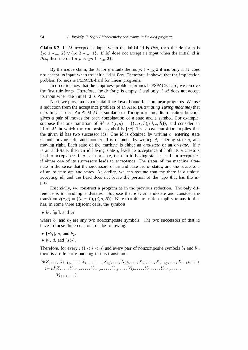
Next, we prove an exponential-time lower bound for nonlinear programs. We usea reduction from the acceptance problem of an ATM (Alternating Turing machine) thatuses linear space. An ATM M is similar to a Turing machine. Its transition functiongives a pair of moves for each combination of a state and a symbol. For example,suppose that one transition of M is δ(c, q) = {(a, r,L), (d, s,R)}, and consider anid of M in which the composite symbol is [qc]. The above transition implies thatthe given id has two successor ids: One id is obtained by writing a, entering stater, and moving left; and another id is obtained by writing d, entering state s, andmoving right. Each state of the machine is either an and-state or an or-state. If qis an and-state, then an id having state q leads to acceptance if both its successorslead to acceptance. If q is an or-state, then an id having state q leads to acceptanceif either one of its successors leads to acceptance. The states of the machine alter-nate in the sense that the successors of an and-state are or-states, and the successorsof an or-state are and-states. As earlier, we can assume that the there is a uniqueaccepting id, and the head does not leave the portion of the tape that has the in-put.

Essentially, we construct a program as in the previous reduction. The only dif-ference is in handling and-states. Suppose that q is an and-state and consider thetransition δ(c, q) = {(a, r,L), (d, s,R)}. Note that this transition applies to any id thathas, in some three adjacent cells, the symbols

• b1, [qc], and b2,

where b1 and b2 are any two noncomposite symbols. The two successors of that idhave in those three cells one of the following:

• [rb1], a, and b2,

• b1, d, and [sb2].

Therefore, for every i (1 < i < n) and every pair of noncomposite symbols b1 and b2,there is a rule corresponding to this transition:

id(Z, . . . ,Xi−1,u, . . . ,Xi−1,v, . . . ,Xi,j , . . . ,Xi,k, . . . ,Xi,l, . . . ,Xi+1,g, . . . ,Xi+1,h, . . .)

:− id(Z, . . . ,Yi−1,u, . . . ,Yi−1,v, . . . ,Yi,j , . . . ,Yi,k, . . . ,Yi,l, . . . ,Yi+1,g, . . . ,

Yi+1,h, . . .)


id(Z, . . . ,Ti−1,u, . . . ,Ti−1,v, . . . ,Ti,j , . . . ,Ti,k, . . . ,Ti,l, . . . ,Ti+1,g, . . . ,

Ti+1,h, . . .),

e(Z,Yi−1,v), e(Z,Yi,l), e(Z,Yi+1,g),

e(Z,Ti−1,u), e(Z,Ti,k), e(Z,Ti+1,h),

e(Z,Xi−1,u), e(Xi−1,v,Z),

e(Z,Xi,j), e(Xi,k,Z), e(Xi,l,Z),

e(Z,Xi+1,g), e(Xi+1,h,Z).

In the above rule, subscripts denote symbols as follows:

• j denotes [qc], k denotes d, and l denotes a,

• u denotes b1, and v denotes [rb1],

• g denotes b2, and h denotes [sb2].

Every column 〈e, f〉 of id that is not shown explicitly has the same variable, denotedas Xe,f , in all three atoms of id. As earlier, the EDB predicate e satisfies e: 1 ≺mc 2.

In order to generate a nonempty disjunct in the head, there must be an i (1 <i < n) and two disjuncts CPos1 and CPos2 for the first and second atoms of id in thebody, respectively, such that:

• Pos1 is an id that has the symbols [rb1], a, and b2 in cells i − 1, i, and i + 1,respectively (this requirement is enforced by the first line of e atoms in the body).

• Pos2 is an id that has the symbols b1, d, and [sb2] in cells i − 1, i, and i + 1,respectively (this requirement is enforced by the second line of e atoms).

• Pos1 and Pos2 must be equal in all cells other than i−1, i, and i+1 (this requirementis enforced, since the two atoms of id in the body have the same variables in allcolumns of those cells).

If all of the above requirements are met, then a disjunct is generated for the head, suchthat it has b1, [qc], and b2 in cells i− 1, i, and i+ 1, respectively, and is equal to Pos1and Pos2 in all other cells.

It is important to observe that the restrictions imposed by the e atoms in eachone of the last three lines (of the above rule) do not force a variable to be both greaterthan and less than Z. If that could happen, it would mean that a composite symbol isidentical to a noncomposite symbol, which is impossible.

Or-states are handled as in the previous reduction, that is, each one of the twomoves out of an or-state yields the same linear rule as in the previous reduction. Thereare also rules for predicate p, based on the initial and accepting ids, as in the previousreduction. Therefore, the dc for predicate id has a disjunct of the form CPos if andonly if Pos is an id of M that leads to acceptance. The rest of the proof follows as inthe previous case. �


Note that the above proof does not require constants in the rules, and the numberof subgoals in each rule is bounded. The arity, however, is unbounded. Moreover, thetheorem remains true even if we consider linear orders instead of strict partial orders.

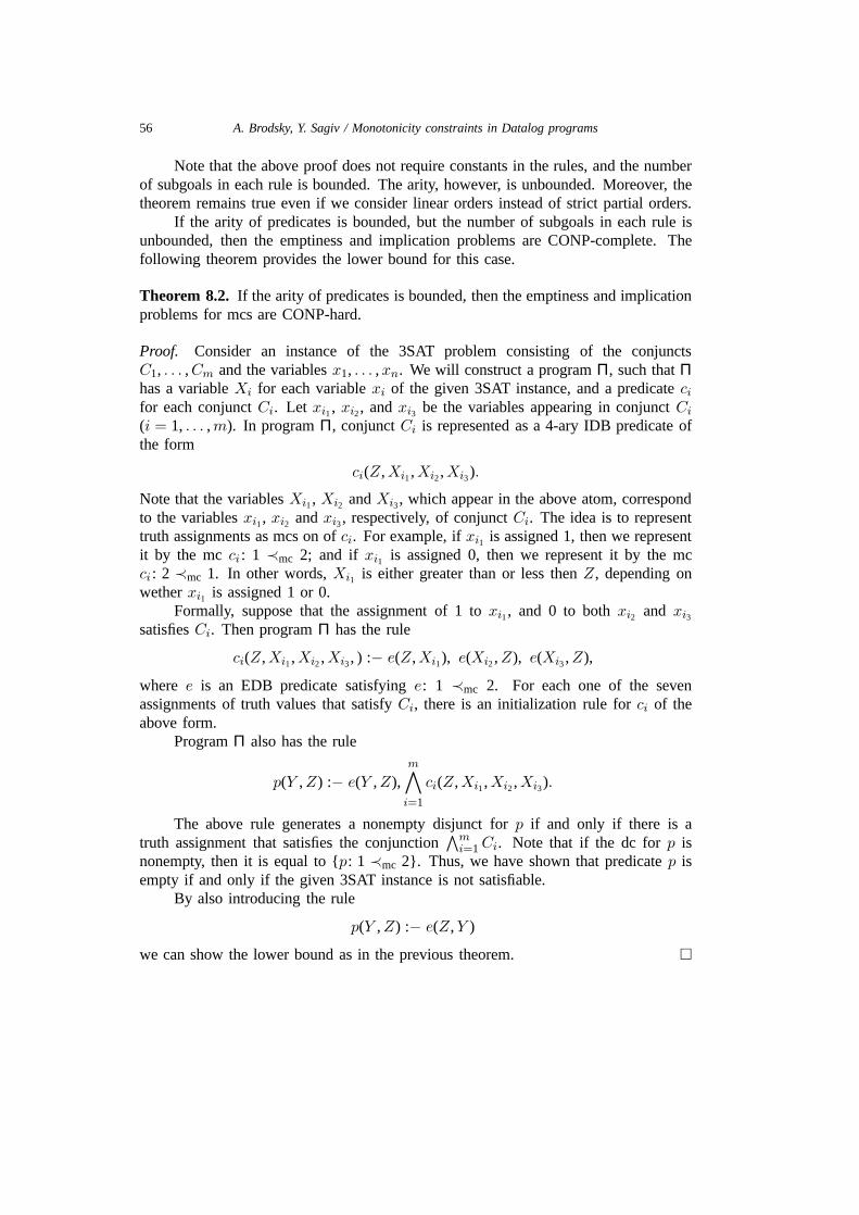
If the arity of predicates is bounded, but the number of subgoals in each rule isunbounded, then the emptiness and implication problems are CONP-complete. Thefollowing theorem provides the lower bound for this case.

Theorem 8.2. If the arity of predicates is bounded, then the emptiness and implicationproblems for mcs are CONP-hard.

Proof. Consider an instance of the 3SAT problem consisting of the conjunctsC1, . . . ,Cm and the variables x1, . . . ,xn. We will construct a program Π, such that Πhas a variable Xi for each variable xi of the given 3SAT instance, and a predicate cifor each conjunct Ci. Let xi1 , xi2 , and xi3 be the variables appearing in conjunct Ci(i = 1, . . . ,m). In program Π, conjunct Ci is represented as a 4-ary IDB predicate ofthe form

ci(Z,Xi1 ,Xi2 ,Xi3 ).

Note that the variables Xi1 , Xi2 and Xi3 , which appear in the above atom, correspondto the variables xi1 , xi2 and xi3 , respectively, of conjunct Ci. The idea is to representtruth assignments as mcs on of ci. For example, if xi1 is assigned 1, then we representit by the mc ci : 1 ≺mc 2; and if xi1 is assigned 0, then we represent it by the mcci : 2 ≺mc 1. In other words, Xi1 is either greater than or less then Z, depending onwether xi1 is assigned 1 or 0.

Formally, suppose that the assignment of 1 to xi1 , and 0 to both xi2 and xi3satisfies Ci. Then program Π has the rule

ci(Z,Xi1 ,Xi2 ,Xi3 , ) :− e(Z,Xi1), e(Xi2 ,Z), e(Xi3 ,Z),

where e is an EDB predicate satisfying e: 1 ≺mc 2. For each one of the sevenassignments of truth values that satisfy Ci, there is an initialization rule for ci of theabove form.

Program Π also has the rule

p(Y ,Z) :− e(Y ,Z),m∧i=1

ci(Z,Xi1 ,Xi2 ,Xi3).

The above rule generates a nonempty disjunct for p if and only if there is atruth assignment that satisfies the conjunction

∧mi=1Ci. Note that if the dc for p is

nonempty, then it is equal to {p: 1 ≺mc 2}. Thus, we have shown that predicate p isempty if and only if the given 3SAT instance is not satisfiable.

By also introducing the rule

p(Y ,Z) :− e(Z,Y )

we can show the lower bound as in the previous theorem. �


We do not know what is the complexity when the arity of all IDB predicatesis less than 4. However, if both the arity of IDB predicates and the number of IDBatoms in the body of each rule are bounded, then the algorithm is polynomial.

Interestingly, determining whether all IDB predicates are weakly safe is in poly-nomial time.

In summary, the results of this paper are of theoretical interest and also applicable.From the theoretical point of view, the paper proved the decidability of the entailementproblem for disjunctions of conjunctions of monotonicity and equility constraints, i.e.,the disjunctive constraints; and provided an effective procudure for finding sound andcomplete disjunctive constraints entailed in a Datalog program. It also showed the tightlower complexity bounds for the entailment problem. From the applicability point ofview, the results of the paper allow to prove that the problem of top-down termina-tion in Datalog programs, given monotonicity and equality constraints for extensionalpredicates, is decidable [3], extending the results of [1].

References

[1] F. Afrati, C.H. Papadimitriou, G. Papageorgiou, A. Roussou, Y. Sagiv and J.D. Ullman, On theconvergence of query evaluation, to appear in J. Comput. System Sci.

[2] A. Brodsky and Y. Sagiv, Inference of monotonicity constraints in Datalog programs, in: Proc. 10thACM SIGACT-SIGART-SIGMOD Symposium on Principles of Database Systems, Philadelphia, PA(1989).

[3] A. Brodsky and Y. Sagiv, On termination of Datalog programs, in: Proc. 19th Internation Conferenceon Deductive and Object-Oriented Databases, Japan (1989).

[4] M. Kifer, R. Ramakrishnan and A. Silberschatz, An axiomatic approach to deciding query safety indeductive databases, in: Proc. 7th ACM Symp. on Principles of Database Systems, Austin (1988)pp. 52–60.

[5] R. Krishnamurthy, R. Ramakrishnan and O. Shmueli, A framework for testing safety and effectivecomputability of extended datalog, in: Proc. ACM Symp. on Management of Data, Chicago (1988)pp. 154–163.

[6] R. Ramakrishnan, F. Bancilhon and A. Silberschatz, Safety of recursive Horn clauses with infiniterelations, in: Proc. 6th ACM Symp. on Principles of Database Systems, San Diego (1987) pp. 328–339.

[7] J.D. Ullman and A. Van Gelder, Efficient tests for top-down termination of logical rules, Journal ofthe ACM 35 (1988) 345–373.

Inference of monotonicity constraints in datalog programs

Documents