Monetary Policy, Leverage, and Bank Risk-Taking�
Giovanni Dell�AricciaIMF and CEPR
Luc LaevenIMF and CEPR
Robert MarquezBoston University
October 2010
Abstract
We provide a theoretical foundation for the claim that prolonged periods of easy monetaryconditions increase bank risk taking. The net e¤ect of a monetary policy change on bankmonitoring (an inverse measure of risk taking) depends on the balance of three forces: interestrate pass-through, risk shifting, and leverage. When banks can adjust their capital structures,a monetary easing leads to greater leverage and lower monitoring. However, if a bank�s capitalstructure is �xed, the balance depends on the degree of bank capitalization: when facing apolicy rate cut, well capitalized banks decrease monitoring, while highly levered banks increaseit. Further, the balance of these e¤ects depends on the structure and contestability of thebanking industry, and is therefore likely to vary across countries and over time.
�The views expressed in this paper are those of the authors and do not necessarily represent those of the IMF.We thank Olivier Blanchard, Stijn Claessens, Gianni De Nicolo�, Hans Degryse, Kenichi Ueda, Fabian Valencia, andseminar participants at Boston University, Harvard Business School, Tilburg University, the Dutch Central Bank,and the IMF for useful comments and discussions. Address for correspondence: Giovanni Dell�Ariccia, IMF, 700 19thStreet NW, Washington, DC, USA. [email protected]

1 Introduction
The recent global �nancial crisis has brought the relationship between monetary policy and bank
risk taking to the forefront of the economic policy debate. Many observers have blamed loose
monetary policy for the credit boom and the ensuing crisis in the late 2000s, arguing that, in the
run up to the crisis, low interest rates and abundant liquidity led �nancial intermediaries to take
excessive risks by fueling asset prices and promoting leverage. The argument is that had monetary
authorities raised interest rates earlier and more aggressively, the consequences of the bust would
have been much less severe. More recently, a related debate has been raging on whether continued
exceptionally low interest rates are setting the stage for the next �nancial crisis.1
Fair or not, these claims have become increasingly popular both in academia and in the business
press. Surprisingly, however, the theoretical foundations for these claims have not been much
studied and hence are not well understood. Macroeconomic models have typically focused on
the quantity rather than the quality of credit (e.g. the literature on the bank lending channel)
and have mostly abstracted from the notion of risk. Papers that consider risk (e.g., �nancial
accelerator models in the spirit of Bernanke and Gertler, 1989) explore primarily how changes in
the stance of monetary policy a¤ects the riskiness of borrowers rather than the risk attitude of
the banking system. In contrast, excessive risk-taking by �nancial intermediaries operating under
limited liability and asymmetric information has been the focus of a large banking literature which,
however, has largely ignored monetary policy.2 This paper is an attempt to �ll this gap.
We develop a model of �nancial intermediation where banks can engage in costly monitoring
to reduce the credit risk in their loan portfolios. Monitoring e¤ort and the pricing (i.e., interest
rates) of bank assets and liabilities are endogenously determined and, in equilibrium, depend on a
benchmark monetary policy rate. We obtain three main �ndings. First, for the case where a bank�s
capital structure is �xed exogenously, we �nd that the e¤ects of monetary policy changes on bank
monitoring and, hence, portfolio risk critically depend on a bank�s leverage: a monetary easing will
lead highly capitalized banks to monitor less, while the opposite is true for poorly capitalized banks.
1See, for example, Rajan (2010), Taylor (2009), or Borio and Zhu (2008).2Diamond and Rajan (2009) and Farhi and Tirole (2009) are recent exceptions, although these deal with the
e¤ects of expectations of a �macro�bailout rather than the implications of the monetary stance. Reviews of the olderliterature are in Boot and Greenbaum (1993), Bhattacharya, Boot, and Thakor (1998), and Carletti (2008).
1

We then endogenize banks�capital structures by allowing them to adjust their capital holdings in
response to monetary policy changes. For this case we �nd that a cut in the policy rate will lead
banks to increase their leverage. Re�ecting this increase in leverage, our third main �nding is that
once leverage is allowed to be optimally chosen, a policy rate cut will unambiguously lower bank
monitoring and increase risk taking.
These results are consistent with the evidence collected by a growing empirical literature on
the e¤ects of monetary policy on risk-taking (see, for example, Maddaloni and Peydró, 2010 and
Ioannidou et al., 2009; Section 2 gives a brief survey). A negative relationship between bank risk
and the real policy rate is also evident in data from the U.S. Terms of Business Lending Survey,
as graphically illustrated in Figure ??. In this �gure, bank risk is measured using the weighted
average internal risk rating assigned to loans by banks from the U.S. Terms of Business Lending
Survey3 and the real policy rate is measured using the nominal federal funds rate adjusted for
consumer price in�ation.4 Both variables are detrended by deducting their linear time trend and
we use quarterly data from the second quarter of 1997 until the fourth quarter of 2008.
Our model is based on two standard assumptions. First, banks are protected by limited liability
and choose the degree to which to monitor their borrowers or, equivalently, choose the riskiness
of their portfolios. Since monitoring e¤ort is not observable, a bank�s capital structure has a
bearing on its risk-taking behavior. Second, monetary policy a¤ects the cost of a bank�s liabilities
through changes in the risk-free rate. Under these two assumptions, we show that the balance of
three coexisting forces - interest-rate pass-through, risk shifting, and leverage - determines how
monetary policy changes a¤ect a bank�s risk taking.
The �rst is a pass-through e¤ect that acts through the asset side of a bank�s balance sheet.
In our model, monetary easing reduces the policy rate, which is then re�ected in a reduction of
the interest rate on bank loans. This, in turn, reduces the bank�s gross return conditional on
3The U.S. Terms of Business Lending Survey, which is a quarterly survey on the terms of business lending of astrati�ed sample of about 400 banks conducted by the U.S. Federal Reserve Bank. The survey asks participatingbanks about the terms of all commercial and industrial loans issued during the �rst full business week of the middlemonth in every quarter. The publicly available version of this survey encompasses an aggregate version of the termsof business lending, disaggregated by type of banks. Loan risk ratings vary from 1 to 5 and are increasing in risk.We use the weighted average risk rating score aggregate across all participating banks as measure of bank risk.
4The e¤ective federal funds rate is a volume-weighted average of rates on trades arranged by major brokers andcalculated daily by the Federal Reserve Bank of New York using data provided by the brokers. As in�ation rate weuse the three-month average change in the U.S. consumer price index.
2

Figure 1: U.S. bank risk and the real federal funds rate
2.4
2.6
2.8
33.
23.
4R
isk
of lo
ans
(det
rend
ed)
-2 0 2 4 6Real Federal Funds Rate (detrended) (in %)
its portfolio repaying, reducing the incentive for the bank to monitor. This e¤ect is akin to the
portfolio reallocation e¤ect present in portfolio choice models. In these models, when monetary
easing reduces the real yield on safe assets, banks will typically increase their demand for risky
assets.5
Second, there is a standard risk-shifting e¤ect that operates through the liability side of a bank�s
balance sheet. Monetary easing lower the costs of a bank�s liabilities. Everything else equal, this
increases a bank�s pro�t when it succeeds and thus creates an incentive to limit risk taking in
order to reap those gains. The extent of this e¤ect, however, depends critically on the degree of
limited liability protection a¤orded to the bank.6 To see why, consider a fully leveraged bank that
is �nanced entirely through deposits/debt. Under limited liability, this bank will su¤er no losses
in case of failure. A policy rate cut will increase the bank�s expected net return on all assets by
lowering the rate it has to pay on deposits. The bank can maximize this e¤ect by reducing the risk
of its portfolio, choosing a safer portfolios for which there is a higher probability the bank will have
to repay depositors. In contrast, for a bank fully funded by capital, the e¤ect of a decrease in the
5The exception would be banks with decreasing absolute risk aversion who, instead, would decrease their holdingsof risky assets (Fishburn and Porter, 1976).
6This is similar to what happens in models that study the e¤ects of competition for deposits on bank stability(Hellmann, Murdoch, and Stiglitz, 2000, Matutes and Vives, 2000, Cordella and Levy-Yeyati , 2003).
3

cost of its liabilities will, all other things equal, increase the expected net return uniformly across
portfolios and have little or no e¤ect on the bank�s risk choices.
When banks�capital structures are exogenously determined, the net e¤ect of a monetary policy
change on bank monitoring depends on the balance of these two e¤ects. This, in turn, depends on a
bank�s capital structure as well as the structure of the market in which it operates. The risk-shifting
e¤ect is stronger the more bene�cial is the limited liability protection to the bank. This e¤ect is
therefore greatest for fully leveraged banks, and is lowest for banks with zero leverage who as a
result have no limited liability protection. In contrast, the magnitude of the pass-through e¤ect
depends on how policy rate changes are re�ected in changes to lending rates. Thus, the magnitude
of this e¤ect depends on the market structure of the banking industry: it is minimal in the case of
a monopolist facing an inelastic demand function, when the pass-through onto the lending rate is
zero; and it is maximal in the case of perfect competition, when lending rates fully re�ect policy
rate changes. It follows that the net e¤ect of a monetary policy change may not be uniform across
times, banking systems or individual banks. Following a policy rate cut, monitoring will decrease
when leverage is low and increase when leverage is high. The position of this threshold level of
leverage will, in turn, depend on the market structure of the banking industry.
By contrast, a third force comes into play once we allow banks to optimally modify their capital
structure in response to a monetary policy change. On the one hand, banks have an incentive to be
levered since holding capital is costly. On the other hand, capital serves as a commitment device
to limit risk taking and helps reduce the cost of debt and deposits. Banks with limited liability
tend to take excessive risk since they do not internalize the losses they impose on depositors and
bondholders. Bank capital reduces this agency problem: the more the bank has to lose in case of
failure, the more it will monitor its portfolio and invest more prudently. When investors cannot
observe a bank�s monitoring but can only infer its equilibrium behavior, higher capital (i.e., lower
leverage) will lower their expectations of a bank�s risk-taking and, thus, reduce the bank�s cost of
deposits and debt. Given that a policy rate cut reduces the agency problem associated with limited
liability, it follows that the bene�t from holding capital will also be reduced. In equilibrium,
therefore, lower policy rates will be associated with greater leverage. This result provides a simple
micro-foundation for the empirical regularities documented in recent papers, such as in Adrian and
4

Shin (2009). The addition of this leverage e¤ect tilts the balance of the other two e¤ects: all else
equal, more leverage means more risk taking. Our model�s unambiguous prediction when banks�
capital structures are endogenous is consistent with the claim that monetary easing leads to greater
risk taking.
Our contribution to the existing literature is twofold. First, we provide a model that isolates
the e¤ect of monetary policy changes on bank risk tasking independently of other macroeconomic
considerations related to asset values, liquidity provision, etc. The model provides a theoretical
foundation for some of the regularities recently documented in the empirical literature, including
the inverse relationship between monetary conditions and leverage, and the tendency for banks to
load up on risk during extended periods of loose monetary policy. While our treatment of monetary
policy is obviously minimal (we take monetary policy as exogenous and abstract from other e¤ects
linked to the macroeconomic cycle), our paper can help bridge the gap between macroeconomic and
banking models. Second, our framework can help reconcile the somewhat dichotomous predictions
of two important strands of research: the literature on the �ight to quality and that on risk shifting
linked to limited liability. The paper also contributes to the ongoing policy debate on whether
macroprudential tools should complement monetary policy to safeguard macro�nancial stability.
We discuss this issue further in the concluding section.
The paper proceeds as follows: Section 2 presents a brief survey of related theoretical and
empirical work. Section 3 introduces the model and examines the equilibrium when the bank
capital structure is exogenous. Section 4 solves the endogenous capital structure case. Section 5
examines the role of market structure, while Sections 6 and ?? present some numerical examples
and stylized facts. Section 7 concludes. Proofs are mostly relegated to the appendix.
2 Related Literature
Our paper is related to a well established literature studying the e¤ects of monetary policy changes
on credit markets. The literature on �nancial accelerators posits that monetary policy tightening
leads to more severe agency problems by depressing borrowers�net worth (see models in the spirit
of Bernanke and Gertler, 1989, and Bernanke et al., 1996). The result is a �ight to quality: �rms
more a¤ected by agency problems will �nd it harder to obtain external �nancing. However, this
5

says little about the riskiness of the marginal borrower that obtains �nancing because monetary
tightening increases agency problems across the board, not just for �rms that are intrinsically more
a¤ected by agency problems. Thakor (1996) focuses on the quantity rather than the quality of
credit. Yet, his model has implications for bank risk taking. In Thakor (1996), banks can invest
in government securities or extend loans to risky entrepreneurs. The impact of monetary policy on
the quantity of bank credit and thus on the riskiness of the bank portfolio depends on its relative
e¤ect on the bank intermediation margin on loans and securities. While the impact on portfolio
risk is not explicitly studied, if monetary easing were to reduce the rate on securities more than
that on deposits, the opportunity cost of extending loans would fall and the portion of a bank�s
portfolio invested in loans would increase; otherwise, the opposite would happen.
Rajan (2005) identi�es in the �search for yield� a related, but di¤erent, mechanism through
which monetary policy changes may a¤ect risk taking. He argues that �nancial institutions may
be induced to switch to riskier assets when a monetary policy easing lowers the yield on their
short-term assets relative to that on their long-term liabilities. This is a result of limited liability.
If yields on safe assets remain low for a prolonged period, continued investment in safe assets will
mean that a �nancial institution will need to default on its long-term commitments. A switch
to riskier assets (and higher yields) may increase the probability that it will be able to match
its obligations. Dell�Ariccia and Marquez (2006a) �nd that when banks face an adverse selection
problem in selecting borrowers, monetary policy easing may lead to a credit boom and lower lending
standards. This is because banks�incentives to screen out bad borrowers are reduced when their
cost of funds is lowered.
More recently, Farhi and Tirole (2009) and Diamond and Rajan (2009) have examined the
role of �macro bailouts� and collective moral hazard on banks� liquidity decisions. When banks
expect a strong policy response by the monetary authorities should a large negative shock occur (a
mechanism often referred to as the �Greenspan put�), they will tend to take on excessive liquidity
risk. This behavior, in turn, will increase the likelihood that the central bank will indeed respond
to a shock by providing the necessary liquidity to the banking system. Unlike in this paper, their
focus is on the reaction function of the central bank (the policy regime) rather than on the policy
stance. Agur and Demertzis (2010) present a reduced form model of bank risk taking to focus on
6

how monetary policymakers should balance the objectives of price stability and �nancial stability.
Drees et al. (2010) �nd that the relationship between the policy rate and risk taking depends on
whether the primary source of risk is the opaqueness of a security or the idiosyncratic risk of the
underlying investment.
Our paper also relates to a large theoretical literature examining the e¤ects of limited liability,
leverage, and deposit rates on bank risk taking behavior. Several papers (for example, Matutes
and Vives, 2000, Hellmann, Murdoch, and Stiglitz, 2000, Cordella and Levy-Yeyati, 2000, Repullo,
2004, and Boyd and De Nicolo�, 2005) have focused on how competition for deposits (i.e., higher
deposit rates) exacerbates the agency problem associated with limited liability and may ine¢ ciently
increase bank risk taking.7 This e¤ect is similar to the risk-shifting e¤ect identi�ed in this paper:
more competition for deposits increases the equilibrium deposit rate, compressing intermediation
margins and thus reducing a bank�s incentives to invest in safe assets.
The framework we use is based on Dell�Ariccia and Marquez (2006b) and Allen, Carletti, and
Marquez (2010). In particular, the latter shows how banks may choose to hold costly capital to
reduce the premium demanded by depositors. They, however, ignore the e¤ects of monetary policy
and do not examine how leverage moves in response to policy rate changes. Our result that leverage
is decreasing in the policy rate is also related to that in Adrian and Shin (2008). In their paper,
leverage is limited by the moral hazard induced by the underlying risks in the environment. In
our model, an increase in the policy rate exacerbates the agency problem associated with limited
liability, which in turn leads to a reduction in leverage.
Finally, there is a small, but growing, empirical literature that links monetary policy and bank
risk taking. For example, Lown and Morgan (2006) show that credit standards in the U.S. tend
to tighten following a monetary contraction. Similarly, Maddaloni and Peydró (2010) �nd that
credit standards tend to loosen when overnight rates are lowered. Moreover, using Taylor rule
residuals, they �nd that holding rates low for prolonged periods of time softens lending standards
even further. Similarly, Altunbas et al. (2010) �nd evidence that �unusually� low interest rates
over an extended period of time contributed to an increase in banks�risk-taking. Jimenez et al.
(2008) and Ioannidou, Ongena, and Peydró (2009) use detailed information on borrower quality
7Boyd and De Nicolo�(2005) also show that when moral hazard on the borrowers side is taken into account, theresult may be reversed.
7

from credit registry databases for Europe and Bolivia. They �nd a positive association between
low interest rates at loan origination and the probability of extending loans to borrowers with bad
or no credit histories (i.e., risky borrowers).
3 A Simple Model of Bank Risk Taking
Banks face a negatively sloped demand function for loans, L(rL), where rL is the gross interest
rate the bank charges on loans. We assume for tractability that the demand function is linear,
L = A� brL. In section 5, we examine the impact of alternative market structures.8
Loans are risky and a bank�s portfolio needs to be monitored to increase the probability of
repayment. The bank is endowed with a monitoring technology, allowing the bank to exert mon-
itoring e¤ort q which also represents the probability of loan repayment. This monitoring e¤ort
entails a cost equal to 12cq
2 per dollar lent.9 An alternative interpretation of this assumption is
that banks have access to a continuum of portfolios characterized by a parameter q 2 [0; 1], with
returns rL � 12cq and probability of success q.
10
Banks fund themselves with two di¤erent types of liabilities. A portion k of a bank�s liabilities
represents a cost irrespective of the bank�s pro�t, while a portion 1 � k is repaid only when the
bank succeeds. Consistent with other existing models, k can represent the portion of bank assets
�nanced with bank equity or capital. In this case, 1 � k would be interpreted as the fraction of
the bank�s portfolio �nanced by deposits. However, k can be also interpreted more generally as an
inverse measure of the degree of limited liability protection accorded to banks. For now, we treat k
as exogenous. In Section 4, we examine the case where banks can adjust k in response to a change
in monetary policy.
For simplicity, we assume that the deposit rate is �xed and equal to the policy rate, rD = r�.
(We will relax this assumption later.) This is consistent with the existence of deposit insurance,
8The assumption of a downward sloping demand curve for loans is supported by broad empirical evidence (e.g.,Den Haan, Sumner, and Yamashiro, 2007). More generally, the pass-through will depend on the cost structure ofbank liabilities, including the proportion of retail versus wholesale deposits (Flannery, 1982). Berlin and Mester(1999) show that markups on loans decrease as market rates increase, implying that as market rates increase, thereis less than a one for one increase in loan rates.
9For a model in the same spirit but where banks choose among portfolios with di¤erent risk/return characteristics,see Cordella and Levy-Yeyati (2003).10This latter interpretation correspond to the classic risk shifting problem between bondholders and shareholders,
in that shareholder can choose between investments that have a lower probability of success, but that payo¤ moreconditional on success.
8

for instance. Equity, however, is more costly, with a yield rE = r� + �, with � � 0, which is
consistent with an equity premium as a spread over the risk-free rate. Alternatively, the cost rE
can be interpreted as the opportunity cost for shareholders of investing in the bank.11
We structure the model in two stages. For a �xed policy rate r�, in stage 1 banks choose the
interest rate to charge on loans, rL. In the second stage, banks then choose how much to monitor
their portfolio, q.
3.1 Equilibrium when Leverage is Exogenous
We solve the model by backward induction, starting from the last stage. The bank�s expected pro�t
can be written as:
� =
�q(rL � rD(1� k))� rEk �
1
2cq2�L(rL); (1)
which re�ects the fact that the bank�s portfolio repays with probability q. When the bank succeeds,
it receives a per-loan payment of rL and earns a return rL � rD(1 � k) after repaying depositors.
When it fails, it receives no revenue, but, because of limited liability, does not need to repay
depositors. The term rEk represents the cost of equity to the bank or, equivalently, the opportunity
cost of bank shareholders, which is borne irrespective of the bank�s revenue.
Taking the loan rate rL as given, the �rst order condition for bank monitoring can be written
as@�q(rL � rD(1� k))� rEk � 1
2cq2�
@qL(rL) = 0;
which implies
bq = min�rL � rD (1� k)c
; 1
�: (2)
Since rD = r�, we obtain immediately from (2) that the direct (i.e., for a given lending rate) e¤ect
of a policy rate hike on bank monitoring is non-positive, @bq@r� � 0. This is consistent with most of
the literature on the e¤ects of deposit competition on risk taking (see for example Hellmann et al.,
2000). One way to interpret this result is that the short-term incentives banks with severe maturity
mismatches have to monitor will be reduced by an unexpected increase in the policy rate.
11We assume that the premium on equity, �, is independent of the policy rate r�. This is consistent with our goal toisolate the e¤ect of an exogenous change in the stance of monetary policy. However, from an asset pricing perspectivethese are likely to be correlated through underlying common factors which may drive the risk premium as well as therisk free rate. Our results continue to hold as long as the within period correlation between � and r� is su¢ cientlydi¤erent from (positive) one.
9

We can now solve the �rst stage of the model where banks choose the loan interest rate.
Assuming that an interior solution exists, we substitute bq into the expected pro�t function andobtain:12
�(bq) = (rL � rD (1� k))22c
� rEk!L(rL): (3)
Maximizing (3) with respect to the loan rate yields the following �rst order condition:
@�(bq)@rL
= L (rL)rL � rD (1� k)
c+@L (rL)
@rL
(rL � rD (1� k))2
2c� rEk
@L (rL)
@rL= 0: (4)
From (4) we obtain our �rst result.
Proposition 1 There exist a degree of capitalization, ek, such that, for k < ek, bank monitoringdecreases with the monetary policy rate, dbqdr� < 0, while for k > ek it increases with the policy rate,dbqdr� > 0.
The intuition behind this result is that a tightening of monetary policy leads to an increase
in both the interest rate a bank charges on its loans and that it pays on its liabilities. The �rst
e¤ect, which re�ects the pass-through of the policy rate on loan rates, increases the incentives to
monitor. The second e¤ect, the risk-shifting e¤ect, decreases monitoring incentives to the extent
that it applies to liabilities that are repaid only in case of success. Indeed, from 2 is evident that
an increase in the cost of capital a¤ects the bank�s monitoring e¤ort only through its e¤ect on the
lending rate. Thus, for a bank funded entirely through capital, the risk-shifting e¤ect disappears.
In contrast, an increase in the interest rate on deposits will also have a direct negative impact on bq:In addition, a tightening of monetary policy leads to a compression of the intermediation margins,
rL � rD. Thus, for a bank entirely funded with deposits, the risk-shifting e¤ect will dominate. In
between the two extremes of full leverage or zero leverage, the bank�s capital structure determines
the net e¤ect of a monetary policy change on risk taking. Banks with a higher leverage ratio will
react to a monetary policy tightening by taking on more risk, while those with a lower leverage
ratio will do the opposite.
12 It is straightforward to see that there always exist values of c that guarantee an interior solution for q. Later,we demonstrate numerically that an interior solution to the full model, where also bank leverage (k) is endogenous,exists. In other words, there is a wide range of parameter values for which the �rst order conditions characterize theequilibrium.
10

It is worth noting that the results so far are obtained under the assumption that the pricing of
deposits is insensitive to risk (i.e., q), but does re�ect the underlying policy rate r�. This would
be consistent with the existence of deposit insurance, so that depositors are not concerned about
being repaid by the bank, but nevertheless want to receive a return that compensates them for
their opportunity cost, which would be incorporated in the policy rate r�.13 In what follows, we
show that the result in Proposition 1 is not driven by depositors�insensitivity to risk, but rather by
the bank�s optimizing behavior given its desire to maximize its expected return, which incorporates
not only the return conditional on success but also the probability of success.
Assume now that depositors must be compensated for the bank�s expected risk taking. De-
positors cannot directly observe q. However, from observing the capital ratio k they can infer the
bank�s equilibrium monitoring behavior, bq. Given an opportunity cost of r�, depositors will demanda promised repayment rD such that rDE[qjk] = r�, or in other words rD = r�
E[qjk] . The timing is as
before, with the additional constraint that depositors�expectations about bank monitoring, E[qjk],
must in equilibrium be correct, so that E[qjk] = bq(rDjk). It is worth noting that this introducesan incentive for the bank to hold some capital. Equity is more expensive than deposits (or debt),
but it allows the bank to commit to a higher q and thus reduces the yield investors demand on
instruments subject to limited liability (i.e. debt or deposits). We exploit this aspect further in
the next section.
We can now state the following result, which parallels that in Proposition 1.
Proposition 2 Suppose that depositors require compensation for risk, so that rD = r�
E[qjk] . Then
there exist a degree of capitalization, eek, such that, for k < eek, bank monitoring decreases with themonetary policy rate, dbqdr� < 0, while for k > eek it increases with the policy rate, dbq
dr� > 0.
4 Endogenous Capital Structure
So far, we have assumed that the bank�s degree of leverage or capitalization is exogenous. This
setting could apply, for instance, to the case of individual banks that would optimally like to
choose a level of capital below some regulatory minimum. For such banks, changes in the policy
13Keeley (1990) formally shows that when deposits are fully protected by deposit insurance, the supply of depositswill not depend on bank risk.
11

rate would not be re�ected in their capitalization decisions since the regulatory constraint would
be binding. In this section, we extend the model to allow for an endogenous capital structure and
contrast our results with those above for the case of exogenous leverage. As capital structure will
be endogenous, we adopt the framework introduced at the end of the previous section and allow
unsecured investors to demand compensation for the risk they expect to face (in other words, we
eliminate deposit insurance).14
Speci�cally, consider the following extension to the model. At stage 1, banks choose their
desired capitalization ratio k. At stage 2, unsecured investors observe the bank�s choice of k and
set the interest rate they charge on the bank�s liabilities. The last two stages are as before in that
banks choose the lending interest rate and then the extent of monitoring.
4.1 Equilibrium
As before, we solve the model by backward induction. The solutions for the last two stages are
analogous to those in the previous section. At stage three, unsecured investors will demand a
promised return of rD = r�
E[qjk] . As we show below, this provides the bank with an incentive to hold
some capital to reduce the cost of borrowing. Formally, the objective function is to maximize bank
pro�ts with respect to the capital ratio k:
maxk� =
�bq(brL � rD(1� k))� rEk � 12cbq2�L(brL);
subject to
rD =r�
E[qjk] ;
where bq = bq(rL; k) is the equilibrium choice of monitoring induced by the bank�s choice of the
loan rate rL and capitalization ratio k, and brL = brL(k) is the optimal loan rate given k. In otherwords, the bank takes into account the in�uence of its choice of k on its subsequent loan pricing
and monitoring decisions.
The �rst order condition for k can be expressed as
d�
dk=@�
@k+@�
@rL
drLdk
+@�
@q
dq
dk=@�
@k= 0
14 In practice, it may be more realistic to assume that some fraction of bank liabilities are insured or insensitive torisk, while the remaining fraction are uninsured so that their pricing must re�ect the expected amount of risk, suchas for subordinated debt. Allowing for these two kinds of liabilities in no way a¤ects our results, as we illustrate inSection 6, where we incorporate both insured and ininsured deposits into our numerical examples.
12

since the last two terms are zero from the envelope theorem. Substituting, this becomes
d�
dk=
�(rL � q)
@q
@k� (rE � r�)
�L(rL) = 0;
which characterizes the bank�s optimal choice of bk. As we show below in Proposition 3, bk is strictlypositive for a broad range of parameter values.
We can now use this to establish the following result.
Proposition 3 Equilibrium bank leverage decreases with the monetary policy rate: dbkdr� > 0.
The proposition establishes that, when an internal solution bk for the capitalization ratio exists,then bk will be increasing in r�. Put di¤erently, a low monetary policy rate will induce banks to bemore leveraged (i.e., to hold less capital).
A policy rate hike increases the rate the bank has to pay on its debt liabilities and exacerbates
the bank�s agency problem - note that at r� = 0, a limit case where the principal is not repaid at
all, there is no moral hazard and bq = q�. This e¤ect is essentially the same as in the �ight-to-qualityliterature (see for example Bernanke et al., 1989). It follows that as the policy rate increases so
does the bene�t from holding capital, the only commitment device available to the bank to reduce
moral hazard. Put di¤erently, investors will allow banks to be more levered when the policy rate
is low relative to when it is high. A similar result is in Adrian and Shin (2008), where leverage is
a decreasing function of the moral hazard induced by the underlying risks in the environment, and
evidence of this behavior is documented in Adrian and Shin (2009).
The following result characterizes banks�loan pricing decisions as a function of the monetary
policy rate, and will be useful in establishing the next main result.
Lemma 1 When bank leverage, the loan rate, and the level of monitoring are all optimally chosen
with respect to the monetary policy rate r�, the optimal loan rate brL is increasing in r�: dbrLdr� .
The intuition for the lemma is straightforward: when the monetary policy rate increases, this
raises the opportunity cost on all forms of �nancing. Consequently, in equilibrium the rate that
the bank charges on any loans also increases. In other words, there is at least some pass through
of the changes in the bank�s costs of funds onto the price of (bank) credit, which is re�ected in a
higher loan rate.
13

We can now state our next main result:
Proposition 4 When bank leverage is optimally chosen to maximize pro�ts, monitoring will always
increase with the monetary policy rate: dbqdr� > 0.
In contrast to the result in Proposition 1, when bank leverage is endogenous we have that bank
monitoring always increases when the policy rate r� increases. Relative to the case where leverage is
exogenous, here monetary policy tightening a¤ects bank monitoring through the additional channel
of a decrease in leverage, as per Proposition 3. Proposition 4 complements this result along the
dimension of bank monitoring, so that the aggregate e¤ect of an increase in the monetary policy
rate is for banks to be less levered and to take less risk (i.e., monitor more). Conversely, reductions
in r� that would accompany monetary easing should lead to more highly levered banks and reduced
monitoring e¤ort.
It bears emphasizing that the clear cut e¤ect of a change in the monetary policy rate arises
only when banks are able to adjust their capital structures (i.e., k) in response to changes in r�.
Changes in bank leverage are, therefore, an important additional channel through which changes in
monetary policy a¤ect bank behavior. Moreover, Proposition 4 shows that the leverage e¤ect can
be su¢ ciently strong to overturn the direct e¤ect on bank risk taking identi�ed in Proposition 2 for
the case where leverage is exogenously given. At the same time, to the extent that some banks may
be constrained by regulation from adjusting their capital structures (for instance, if their optimal
capital holdings are below the minimum mandated by capital adequacy regulation), we may in
practice observe cross sectional di¤erences in banks�reactions to monetary policy shocks.
5 Extension: The role of market structure
This section examines the e¤ect of alternative assumptions on the structure of the loan market. We
look at two diametrically opposed cases: First, a perfectly competitive credit market, where banks
take the lending rate as given, which is determined by market clearing and a zero pro�t condition
for the banks; and second, a monopolist facing a loan demand function that is perfectly inelastic
up to some �xed loan rate R. This upper limit can be interpreted as either the maximum return
on projects, or as the highest rate consistent with borrowers satisfying their reservation utilities.
14

Under these two extreme structures, we show that our results when leverage is endogenous continue
to hold qualitatively. Speci�cally, when the capital ratio k is endogenously determined, the leverage
e¤ect dominates and monetary easing will increase bank risk taking. If banks are unable to adjust
their capital structures, however, the loan market structure does matter for how monetary policy
a¤ects risk taking. Intuitively, the pass-through of the monetary policy rate on lending rates is
higher the more competitive is the market. It follows that intermediation margins are less sensitive
to monetary policy changes in more competitive markets. And this, in turn, results in a diminished
risk shifting e¤ect and consequently a smaller region of leverage for which monetary easing causes
risk taking to decrease.
5.1 The Perfect Competition Case
Consider the following modi�cation of our model to incorporate perfect competition. At stage 1,
given a �xed policy rate, the lending rate is set competitively so that banks make zero expected
pro�ts in equilibrium. At stage 2, banks choose their desired leverage (or capitalization) ratio k. At
stage 3, unsecured investors observe the bank�s choice of k and set the interest rate they charge on
the bank�s liabilities, rD. And in the last stages, as before, banks choose the extent of monitoring.
Again, we solve the model by backward induction. As for the case where banks have market
power analyzed in Sections 3 and 4, solving for the equilibrium monitoring and imposing rD = r�
E[qjk]
implies, as before
bq = rL +qr2L � 4cr� (1� k)
2c: (5)
We �rst consider the case where k is exogenous. For this case, we impose a zero pro�t condition,
b� = L�bqrL � r� � k� � c
2bq2� = 0;
to obtain rL as a function of r� and k. We can now state the following result.
Proposition 5 In a perfectly competitive market, for a �xed capitalization ratio k, bank monitoring
increases with the monetary policy rate, dbqdr� > 0, for k 2 (0; 1], with dbqdr� = 0 for k = 0.
This result contrasts with that obtained in Propositions 1 and 2 for the case where banks have
market power. There, the e¤ect of a change in monetary policy on risk taking depended on the
15

degree of bank capitalization, k, with decreased risk taking as the monetary policy rate increases
for a su¢ ciently low level of k. Here dbqdr� , the bank�s response to changes in monetary policy in
terms of monitoring, remains non-negative over its entire range, although it is still increasing in
k. This result stems from the fact that the pass-through of the policy rate onto the loan rate is
maximum in the case of perfect competition, and must perfectly re�ect the increase in the policy
rate. It follows that the pass-through e¤ect dominates the risk-shifting e¤ect, so that the region
where dbqdr� < 0 disappears.
We next endogenize the capital ratio k, as in Section 4. Banks maximize
maxk� = L
�bqrL � r� � k� � c
2bq2� ;
which for the case of perfect competition gives
bk = 1� r2L � (r� + �)
cr (r� + 2�)2:
To obtain the lending rate, we impose the zero pro�t condition for banks:
b� = L�bq(bk)rL � r� � bk� � c
2bq2(bk)� = 0: (6)
From (6) we can solve for the equilibrium lending rate, capital, and monitoring as: brL =r 2cr�(r�+2�)2
3r��+(r�)2+2�2,
bk = r��+(r�)2
3r��+(r�)2+2�2, and bq = r r�4(r�+�)2
2c(3r��+(r�)2+2�2). From these we immediately obtain the following
result.
Proposition 6 In a perfectly competitive market, equilibrium bank leverage decreases with the
monetary policy rate: dbkdr� > 0. And, when bank leverage is optimally chosen to maximize pro�ts,
monitoring will always increase with the monetary policy rate: dbqdr� > 0.
This result extends Propositions 3 and 4 to the case of perfect competition and establishes that
even when credit markets are perfectly competitive, monetary easing in equilibrium lead banks to
both hold less capital and take on more risk once one incorporates banks�ability to adjust their
optimal leverage ratios.
5.2 A Monopolist Facing Inelastic Demand
Here, we assume as in the main part of the paper that banks can choose the interest rate to charge,
but also that there is a �xed demand for loans, L, as long as the lending rate does not exceed a
16

�xed value of R. This setting can be interpreted as one where each borrower has a unit demand
for loans and R is the borrower�s reservation loan rate. Demand becomes zero for rL > R. This
eliminates any pricing e¤ects on loan quantity and allows us to focus on a case where the loan rate
is not responsive to changes in the cost of funding since, given the �xed, inelastic demand, it will
always be set at the maximum value of brL = R.We can solve for bq, imposing the condition that rD = r�
E[qjk] , and obtain
bq = R+pR2 � 4cr� (1� k)
2c; (7)
from which we can state the following claim.
Claim 1 For k 2 [0; 1) �xed, a monopolist bank facing a demand function that is perfectly inelastic
for rL � R will always decrease monitoring when the policy rate is raised: dbqdr
���k< 0. For k = 1,
dbqdr
���k= 0.
Proof: From 7 we can immediately write:
dbqdr= � 1� kp
R2 � 4cr� (1� k)< 0:
�
This result stands in stark contrast with what we obtained in Proposition 5 for the case of
perfect competition when leverage is exogenous. There, irrespective of the level of leverage, risk
taking was always decreasing in the policy rate. Here, risk taking is always increasing in the policy
rate. The di¤erence stems precisely from the extent to which the bank passes onto the lending
interest rate changes in its costs stemming from changes in the policy rate. If demand is inelastic,
the pass-through is zero as the lending rate is always held at its maximum, R, and thus cannot
adjust further when the monetary policy rate changes. Therefore, the impact of a change in the
policy rate on monitoring, bq, operates solely through the liability side of the bank balance sheet,reducing the bank�s return in case of success and leading it to monitor less. Put di¤erently, there
is only a risk-shifting e¤ect. By contrast, in the perfect competition case the pass-through is at its
maximum and the impact of a change in r� on the lending rate dominates the risk shifting e¤ect.
17

This result holds in a more general setting. For example, in our main model it can be shown
that the leverage threshold below which a monetary policy tightening leads to an increase in risk-
taking is lower the �atter is the loan demand function. Again, as demand becomes more elastic -
which can be interpreted as the market becoming more competitive - the interest rate pass-through
increases, making the net e¤ect of a change in the policy rate on monitoring more positive.15
To study the e¤ect of a change in monetary policy when the monopolist bank can choose the
capitalization ratio k, we maximize bank pro�ts with respect to k:
maxk� = L
�bqR� r � k� � c
2bq2� :
This gives the �rst order condition
�r�
2� � + r�R
2pR2 � 4cr� (1� k)
= 0;
that has solution bk = 1�R2 � (r� + �)
cr� (r� + 2�)2: (8)
We can substitute the solution bk back into the formula for bq to obtainbq = R (r + �)
c (r + 2�): (9)
It is now immediate that Proposition 6 extends to this case: dbkdr� > 0 and
dbqdr� > 0 when the bank
can adjust its target capital ratio in response to a change in the monetary policy rate.
6 A Numerical Example
In this section, we present some simple numerical simulations of the model. The purpose is twofold.
First, we want to provide an intuitive graphical illustration of the e¤ects identi�ed in this paper.
Second, since most of our analysis relies on internal solutions for several of the choice variables in
the model, the example serves to demonstrate that there is a broad set of parameter values for
which such solutions indeed exist.
For the linear demand function L = A � brL as above, we assume that A = 100 and b = 8.
We also assume that 35 percent of the bank�s liabilities consist of insured deposits and the rest is
15A formal proof for this result can be obtained on request from the authors.
18

Figure 2: Bank monitoring, bq, as a function of the monetary policy rate r� for di¤erent values ofbank capitalization, k.0.951.001.051.101.151.200.850.900.951.00
k=0.0
k=0.3
k=0.6
k=0.9
r*
q^
uninsured and therefore must be priced to re�ect its risk. This is to provide some realism to the
numbers and also to cover both cases considered in our analysis. Finally, we set the monitoring
cost parameter c = 9 and the equity premium, �, to 6 percent.16
Figure 2 illustrates Proposition 1. The equilibrium probability of loan repayment for di¤erent
levels of k is plotted as a function of the policy rate. The chart covers a broad range of real interest
rate values (from negative 10 percent to positive 20 percent) encompassing the vast majority of
realistic cases. From this picture it is easy to see how the response of a bank�s risk taking to a change
in the monetary policy rate depends on its capitalization. For low levels of k, bank monitoring bqdecreases with the policy rate r�, and the opposite happens at high levels.17
When we allow the bank to change is target leverage ratio, an additional e¤ect emerges and the
short-term ambiguity in the relationship between risk-taking and the policy rate is resolved. As
the policy rate increases, so does the agency problem associated with limited liability. The bank�s
response is to decrease its leverage ratio to limit the increase in the interest rate it has to pay
on its uninsured liabilities. Figure 3 describes this relationship. The equilibrium leverage ratio is
plotted against the real policy interest rate. Note that, for illustrative purposes, the chart covers
an extremely wide range of interest rates from minus 100 percent to plus 100 percent, which are
well beyond what typically occurs in practice. At extremely low values of the policy rate (below
minus 15 percent), the agency problem is su¢ ciently small that the bank �nds it optimal to be fully
16An equity premium of 6 percent is consistent with the historical average spread between U.S. stock returns andrisk-free interest rate as reported in Mehra and Prescott (1985).17 In our numerical example, the threshold value for k at which the relationship between the policy rate and bank
risk taking reverses is about 0.55, which is a fairly high capitalization ratio in practice.
19

Figure 3: Optimal bank capitalization, bk, as a function of the real policy interest rate r�.
0.5 1.0 1.5 2.0
0.2
0.4
0.6
r*
k^
levered (more technically, k hits the zero-lower-bound corner solution). For more realistic ranges of
the interest rate, the model admits an internal solution and bank capital k increases with the policy
interest rate. However, the slope of this relationship is decreasing in the policy rate. Eventually,
the relationship becomes �at once it hits its upper bound (this corresponds to bq(k) = 1; see below).Figure 4 illustrates the relationship between the bank�s monitoring e¤ort/probability of repay-
ment and the real policy rate for the case with endogenous leverage. For extremely low values of
the real policy rate (exactly the values for which bk = 0), bank monitoring bq is decreasing in thepolicy rate. The intuition is straightforward. At these levels bk is in a corner (at zero) and does notmove when the policy rate changes. It follows that the result related to a �xed capital structure
applies. And since bk = 0, we obtain that dbqdr� =
dbqdr�
���k=0
< 0. For the most realistic real policy rate
range between minus 10 percent and plus 20 percent, bq admits an internal solution and is increasingin r�. Eventually, at a very high real interest rate (about 80 percent), bq hits its upper bound, whichis exactly when the relationship between bk and r� becomes �at.7 Discussion and Conclusions
This paper provides a theoretical foundation for the claim that prolonged periods of easy monetary
conditions increase bank risk taking. In our model, the net e¤ect of a monetary policy change on
bank monitoring (an inverse measure of risk taking) depends on the balance of three forces: interest
rate pass-through, risk shifting, and leverage. When banks can adjust their capital structures, a
monetary easing leads to greater leverage and lower monitoring. However, if a bank�s capital
20

Figure 4: Equilibrium bank monitoring, bq(bk), as a function of the real policy interest rate.
0.5 1.0 1.5 2.0
0.86
0.88
0.90
0.92
0.94
0.96
0.98
1.00
r*
q^
structure is instead �xed, the balance will depend on the degree of bank capitalization: when facing
a policy rate cut, well capitalized banks will decrease monitoring, while highly levered banks will
increase it. Further, the balance of these e¤ects will depend on the structure and contestability of
the banking industry, and is therefore likely to vary across countries and over time.
There are several potential extensions to our analysis that are useful to discuss. First, we model
monetary policy decisions as exogenous changes in the real yield on safe assets. Of course, this is an
approximation. In particular, we abstract from how central banks respond to the economic cycle
and in�ation pressures when choosing their policy stance. The next step should be to take into
account the role of the interaction of the monetary policy stance with the real cycle in determining
bank risk-taking. A promising avenue in this direction may be to augment the model to examine
how borrowers�incentives change over the cycle.
Another important simplifying assumption is that the cost of equity is independent from the
bank�s leverage. Yet, our results would continue to hold in a more complex setting where the
required return to equity is a increasing in the degree of bank leverage. In this case, it is straight-
forward to see that, everything else equal, equilibrium leverage would be lower than in our base
model since an increase in capitalization would have the additional bene�t of reducing equity costs.
Also, leverage would continue to be decreasing in the policy rate, although the exact shape of this
relationship would depend on the functional form assumed for the cost of equity as a function of
leverage.
A third simpli�cation in the paper is that we focus on credit risk and abstract from other
21

important aspects of the relationship between monetary policy and risk taking, such as liquidity
risk.18 While other frameworks may be better suited to study this issue (see, for example, Farhi and
Tirole, 2009, and Stein, 2010), our model could be adapted to capture risks on the liability side of
the bank�s balance sheet. For instance, banks might choose to �nance themselves through expensive
long-term debt instruments or cheaper short-term deposits, which, however, carry a greater liquidity
risk. In that context, the trade-o¤ for a bank would be between a wider intermediation margin
and a greater risk of failure should a liquidity run ensue. Hence, dynamics similar to those in this
paper could be obtained. We leave all these extensions to future research.
The model has clear testable implications. First, in situations where banks are relatively un-
constrained in raising capital and can adjust their capital structures, the model predicts a negative
relationship between the policy rate (in real terms) and measures of bank risk. Second, in situations
where banks face constraints, such as when their desired capital ratios are already below regulatory
minimums for capital regulation, this negative relationship between the policy rate and bank risk
is less pronounced for poorly capitalized banks and in less competitive banking markets. Third,
the model predicts a negative relationship between the policy rate and bank leverage. While we
provide some simple empirical evidence in support of a negative relationship between policy rate
and bank risk, and policy rate and leverage, we leave more rigorous empirical analysis of these
relationships to future research.
The �ndings in this paper bear on the debate about how to integrate macro-prudential regulation
into the monetary policy framework to meet the twin objectives of price and �nancial stability (see,
for example, Blanchard et al., 2009). Whether a trade o¤ between the two objectives emerges will
depend on the type of shocks the economy is facing. For instance, no trade-o¤ between price and
�nancial stability may exist when an economy nears the peak of a cycle, when banks tend to take
the most risks and prices are under pressure. Under these conditions, monetary tightening will
decrease leverage and risk taking and, at the same time contain price pressures. In contrast, a
trade-o¤ between the two objectives would emerge in an environment, such as that in the runup to
the current crisis, with low in�ation but excessive risk taking. Under these conditions, the policy
18A growing literature focuses on funding liquidity risk of banks and the adverse liquidity spirals that such riskcould generate in the event of negative shocks (see Diamond and Rajan, 2008; Brunnermeier and Pedersen, 2009;and Acharya and Viswanathan, 2010) and on the role of monetary policy in altering bank fragility in the presence ofliquidity risk (Acharya and Naqvi, 2010; and Freixas et al., 2010).
22

rate cannot deal with both objectives at the same time: Tightening may reduce risk-taking, but will
lead to an undesired contraction in aggregate activity and/or to de�ation. Other (macroprudential)
tools are then needed.
In this context, the potential interaction between banking market conditions, monetary policy
decisions, and bank risk-taking implied by our analysis can be seen as an argument in favor of
the centralization of macro-prudential responsibilities within the monetary authority. And the
complexity of this interaction points in the same direction. How these bene�ts balance with the
potential for lower credibility and accountability associated with a more complex mandate and the
consequent increased risk of political interference is a question for future research.
23

8 Appendix
Proof of Proposition 1: Since bq = rL�r�(1�k)c , dbq
dr� =1c
�dbrLdr� � (1� k)
�. To �nd dbrL
dr� , start by
substituting bq = rL�r�(1�k)c into the expected pro�t function, and given rE = r� + �, we obtain
� =
�q(rL � r�(1� k))� rEk �
1
2cq2�L(rL) (10)
=
rL � r� (1� k)
c(rL � r�(1� k))� (r� + �) k �
1
2c
�rL � r� (1� k)
c
�2!L(rL) (11)
=
�1
2c(rL � r� (1� k))2 � k (� + r�)
�L(rL) (12)
The �rst order condition with respect to rL is
@�
@rL=1
c(rL � r� (1� k))L (rL) +
@L (rL)
@rL
�1
2c(rL � r� (1� k))2 � k (� + r�)
�= 0:
De�ne the identity G � @�@rL
= 0. We can now use the Implicit Function Theorem, that dbrLdr� = � @G@r�@G@rL
.
For the denominator, di¤erentiate G with respect to rL to get the following second order condition:
@G
@rL=
1
cL (rL) +
1
c(rL � r� (1� k))
@L (rL)
@rL+@2L (rL)
@r2L
�1
2c(rL � r� (1� k))2 � k (� + r�)
�+@L (rL)
@rL
1
2c(rL � r� (1� k))
Since @2L(rL)@r2L
= 0, this becomes
@G
@rL=1
cL (rL) +
@L (rL)
@rL
3
2c(rL � r� (1� k)) :
We can rewrite the FOC with respect to rL as
L (rL) = �@L (rL)
@rL
1
2(rL � r� (1� k))�
k (� + r�)1c (rL � r� (1� k))
!; (13)
and substitute into @G@rL
to obtain
@G
@rL=1
c
@L (rL)
@rL
�rL � r� (1� k) + c
k
rL � r� (1� k)(� + r�)
�< 0;
which establishes the second order condition as negative.
We can now di¤erentiate G with respect to r�.
@G
@r�= �1
c(1� k)L (rL)�
1
c
@L (rL)
@rL((rL � r� (1� k)) (1� k) + ck) :
24

Using again the �rst order condition expressed as in (13), we can substitute this into the above to
get@G
@r�= �@L (rL)
@rL
(1� k)
12c (rL � r
� (1� k))2 + k (� + r�)(rL � r� (1� k))
!+ k
!> 0;
which, combined with the fact that @G@rL
< 0, establishes that dbrLdr� = � @G@r�@G@rL
> 0: Clearly, as k ! 0,
the expression for @G@r� converges to
@G
@r�= �@L (rL)
@rL
1
2c(rL � r�) > 0:
To sign dbqdr� , however, we need to compare
dbrLdr� to 1:
dbrLdr�
����k=0
= �@G@r�
@G@rL
= ��1c@L(rL)@rL
12 (rL � r
�)
1c@L(rL)@rL
(rL � r�)
=1
2< 1;
so that dbqdr� =
1c
�dbrLdr� � (1� k)
�= 1
c
�12 � 1
�< 0 for k = 0.
At the other extreme, as k ! 1, we have
@G
@r�= �@L (rL)
@rL> 0;
which again establishes that dbrLdr� > 0 for k = 1. Given dbq
dr�
���k=1
= 1cdbrLdr� , we can conclude that
dbqdr� > 0 for k = 1.
By continuity, there must exist a value of k, ek, such that dbqdr� < 0 for k < ek, and dbq
dr� > 0 for
k > ek. The �nal step is to show that such a value is unique. Given our assumption of a linear
demand function, we can without loss of generality write this as L (rL) = A � brL. We can now
substitute for bq into the bank�s pro�ts to obtain� =
c
2
�rL � r�(1� k)
c
�2� k (r� + �)
!(A� brL):
From this we obtain the FOC with respect to rL,
@�
@rL= (A� brL)
�rL � r�(1� k)
c
�� b
c
2
�rL � r�(1� k)
c
�2� k (r� + �)
!= 0:
Solving yields
brL = 1
3b
�A+ 2br�(1� k) +
q(A� br�(1� k))2 + 6kb2c (r� + �)
�; (14)
25

and substituting into bq we obtainbq =
�A� br�(1� k) +
q(A� br�(1� k))2 + 6kb2c (r� + �)
�3bc
:
This expression for bq is clearly increasing in k, and is decreasing in r� for values of k near 0, andincreasing in r� for values of k near 1. Tedious calculations show that, for value of c such that
bq < 1 (i.e., for which we have an interior solution), in addition we have @2bq@r�@k > 0 for all k 2 (0; 1).
Therefore, there is a unique point ek for which dbqdr� = 0, as desired. �
Proof of Proposition 2: In the absence of deposit insurance, rational depositors will demand
an interest rate commensurate to the expected probability of repayment, rD = r�
E[bq] . Recall that,assuming an interior solution, we have bq = rL�rD(1�k)
c . Since in equilibrium depositors�expectations
must be correct, we can substitute for rD as rD = r�
E[bq] and rearrange to getq2 � rLq + r� (1� k) = 0:
Following Allen et al. (2010), we solve for q and take the larger root:
bq (k) = 1
2c
�rL +
qr2L � 4cr� (1� k)
�: (15)
This implies
dbq (k)dr
����k
=1
2c
0@ drLdr
����k
+�2c(1� k) + rL drL
dr
���kq
r2L � 4cr� (1� k)
1A : (16)
The deposit rate is obtained from the maximization of the bank�s pro�t, and is determined by the
following FOC (after substituting L (rL) = A� brL):
@�
@rL= (A� brL)
�rL � rD(1� k)
c
�� b
c
2
�rL � rD(1� k)
c
�2� k (r� + �)
!= 0:
Solving gives
brL = 1
3b
�A+ 2brD(1� k) +
q(A� brD(1� k))2 + 6kb2c (r� + �)
�: (17)
Di¤erentiating rL with respect to k we obtain
drLdr�
=2
3
drDdr�
(1� k) +bck + 1
3drDdr (1� k) (brD (1� k)�A)q
(A� brD(1� k))2 + 6kb2c (r� + �):
26

Evaluated at k = 1, this expression becomes drLdr� =bcp
A2+6b2c(r�+�)> 0. This immediately implies
that at k = 1, dbq(k)dr� =drLdr�c > 0.
Now consider the case k = 0. At k = 0, drLdr� becomesdrLdr =
13drDdr . Thus we have
drLdr� =
drDdr3 .
And since rD = rbq ,drDdr�
3=1
3
bq � r� dbqdrbq2!:
Plugging this into (16), we get
dbq (k)dr�
=1
2c
0BB@13 bq � r� dbqdrbq2
!+
�2c+ rL 13� bq�r� dbq
drbq2�
qr2L � 4cr�
1CCA ;which solving for dbq(k)dr� yields:
dbq (k)dr�
=bq �rL +qr2L � 4cr� � 6cbq�
r��rL +
qr2L � 4cr�
�+ 6bq2cqr2L � 4cr� : (18)
The denominator of (18) is positive, and remembering that at k = 0,
bq (k) = 1
2c
�rL +
qr2L � 4cr�
�;
we can write the numerator of (18) as
bq (2cbq � 6cbq) = �4bq2 < 0:This tells us that dbq(k)dr� < 0 at k = 0, as desired. �
Proof of Proposition 3: As in Proposition 2, in the absence of deposit insurance, rational
depositors will demand an interest rate commensurate to the expected probability of repayment,
rD =r�
E[bq] . As before, this yields an equilibrium expression for bank monitoring as
bq (k) = 1
2c
�rL +
qr2L � 4cr� (1� k)
�: (19)
Also, again using the fact that in equilibrium we must have rD = r�bq , we can rewrite the pro�tfunction as:
� =
�bqbrL � r�(1� k)� rEk � 12cbq2�L(brL):
27

The �rst order condition with respect to k is
@�
@k=
�r� � rE +
@bq@k(brL � cbq)�L(brL) + @�
@brL @brL@k = 0:
The second term, @�@brL @brL@k , is zero by the envelope theorem, which implies a �rst order condition ofr� � rE +
@bq@k(brL � cbq) = 0: (20)
The second order condition can now be written as
@2�
@k2=@L
@brL @brL@k�r� � rE +
@bq@k(brL � cbq)�+ L(brL)�@bq
@k
�@brL@k
� c@bq@k
�+@2bq@k2
(brL � cbq)� :The �rst term is zero from (20), leaving only
@2�
@k2=@bq@k
�@brL@k
� c@bq@k
�+@2bq@k2
(brL � cbq) : (21)
To sign this expression, we use the following auxiliary result.
Lemma 2 Around the optimal leverage ratio bk, the optimal loan rate brL is increasing in k: @brL@k
���bk >0.
Proof of Lemma 2: From the �rst order conditions with respect to rL we have
@�
@rL= qL (rL) +
@L (rL)
@rL
�bq (rL � rD(1� k))� rEk � 12cbq2�+ @�
@q
@q
@rL= 0:
Since the last term is zero by the envelope theorem, we can write:
bqL (rL) + @L (rL)@rL
�bq (rL � rD(1� k))� rEk � 12cbq2� = 0: (22)
De�ne Z � @�@rL
= 0. Then, using the Implicit Function Theorem we have @brL@k
���bk = � @Z@k@Z@rL
:
@Z
@rL= bq@L (rL)
@rL+ L (rL)
@bq@rL
+ bq@L (rL)@rL
+@2L (rL)
@r2L
�bq (rL � rD(1� k))� rEk � 12cbq2�+
@L (rL)
@rL
�bq (rL � rD(1� k))� rEk � 12cbq2�
@q
@q
@rL;
where the last two terms are zero: the �rst because of the linearity of the loan demand function,
and the second because of the envelope theorem. This means:
@Z
@rL= 2bq@L (rL)
@rL+ L (rL)
@bq@rL
:
28

We can rewrite Z = 0 as
L (rL) = �@L(rL)@rL
�bq (rL � rD(1� k))� rEk � 12cbq2�bq :
Thus
@Z
@rL= 2bq@L (rL)
@rL�
@L(rL)@rL
�bq (rL � rD(1� k))� rEk � 12cbq2�bq @bq
@rL
=1bq�2bq2@L (rL)
@rL� @L (rL)
@rL
�bq (rL � rD(1� k))� rEk � 12cbq2� @bq
@rL
�;
and, since rD is already determined at this stage, we can substitute for bq in the above as bq =rL�rD(1�k)
c and write the second order condition as
@Z
@rL=
1bq @L (rL)@rL
�3
2bq2 + rEk
c
�=
@2�
@r2L=1bq @L (rL)@rL
3
2
�rL � rD(1� k)
c
�2+rEk
c
!< 0;
which veri�es the second order condition.
Now, to compute @Z@k , we �rst write Z in a way that re�ects the equilibrium condition that
rD =r�bq , since rD is determined after k and r� are chosen:
Z = bqL (rL) + @L (rL)@rL
�bqrL � r�(1� k)� rEk � 12cbq2� = 0:
We can now di¤erentiate this to obtain
@Z
@k=
@bq@kL (rL) +
@L (rL)
@rL(r� � rE) +
@L (rL)
@rL(rL � cbq) @bq
@k
=@bq@kL (rL) +
@L (rL)
@rL
��� + (rL � cbq) @bq
@k
�:
However, from (20), the FOC with respect to k, we know that the term in brackets is zero. This
means that, for bq (k) = 12c
�rL +
qr2L � 4cr� (1� k)
�,
@Z
@k=@bq@kL (rL) =
L (rL) r�q
r2L � 4cr� (1� k)> 0:
Thus, @brL@k���bk = � @Z
@k@Z@rL
> 0, as desired. �
We can now use Lemma 2 to establish that, around the equilibrium value of capital bk, @brL@k > 0.From this, it also follows that @bq@k > 0. We therefore need to sign
�@brL@k � c
@bq@k
�. From (19), we can
29

write
c@bq@k
=1
2
@brL@k
+cr� + 1
2@brL@k brLq
r2L � 4cr� (1� k):
Thus
@brL@k�c@bq@k
=1
2
@brL@k�
cr� + 12@brL@k brLq
r2L � 4cr� (1� k)=1
2
@brL@k
0@1� brLqr2L � 4cr� (1� k)
1A� cr�qr2L � 4cr� (1� k)
;
which is negative because brL �qr2L � 4cr� (1� k) for any k � 1. Note as well that@2bq@k2
=@2
@k2
�1
2c
�rL +
qr2L � 4cr� (1� k)
��= �2c (r�)2�q
r2L � 4cr� + 4ckr��3 < 0:
It follows that pro�ts are concave in k.
De�ne now G � @�@k = 0 and H = @2�
@k2< 0. Using the implicit function theorem, we then have
dbkdr�
= �@G@r�
H:
Since the denominator is negative, the sign of dbkdr� will be the same as that of
@G@r� . Note that
r� � rE = r� � (r� + �) = ��. Then, the numerator is
@G
@r�=@��� + @bq
@k (brL � cbq)�@r�
=@bq@k
�@brL@r�
� c @bq@r�
�+ (brL � cbq) @2bq
@k@r�: (23)
The �rst term is positive since @bq@k > 0, @brL@r� > 0, and @bq
@r� < 0. The second term depends on the
sign of @2bq@k@r� , which is given by
@2
@k@r�
�1
2c
�rL +
qr2L � 4cr� (1� k)
��=
r2L � 2cr� (1� k)�r2L � 4cr� (1� k)
� 32
> 0:
It follows that dbkdr� > 0, as desired. �
Proof of Lemma 1: We can write dbrLdr� =
@brL@k
���bk dbkdr� +
dbrLdr�
���bk, where the notation dbrLdr�
���krefers to
the derivative of the equilibrium loan rate with respect to the monetary policy rate, for a given
�xed capital ratio k. As above, @brL@k
���bk is the derivative of the loan rate around the equilibriumlevel of capital, bk. Therefore, we have that the �rst term, @brL@k ���bk dbk
dr� , is positive from Lemma 2 and
Proposition 3. Therefore, the only remaining term to sign is dbrLdr�
���bk. For this, recall again the �rstorder condition for pro�t maximization with respect to rL obtained in (22):
@�
@rL= bqL (rL) + @L (rL)
@rL
�bq (rL � rD(1� k))� rEk � 12cbq2� = 0:
30

We again de�ne Z � @�@rL
= 0. Then, using the Implicit Function Theorem we have drLdr� = �
@Z@r�@Z@rL
.
The denominator we know is negative from the proof of Lemma 2. For the numerator, we have
@Z
@r�=
@bq@r�
L (rL)�@L (rL)
@rL+@L (rL)
@rL(rL � cbq) @q
@r�
=@bq@r�
L (rL)�@L (rL)
@rL
�1� (rL � cbq) @q
@r�
�:
Now, using the fact that bq = 12c
�rL +
qr2L � 4cr� (1� k)
�, we know that
@bq@r�
= � 1� kqr2L � 4cr� (1� k)
:
For ease of exposition, let us de�ne W =qr2L � 4cr� (1� k):We can substitute this into
@Z@r� to
obtain@Z
@r�= �1� k
WL (rL)�
@L (rL)
@rL
�1�
�rL � c
1
2c(rL +W )
���1� kW
��:
We can rewrite Z = 0 as
L (rL) = �@L(rL)@rL
�bqrL � r�(1� k)� rEk � 12cbq2�bq = �
@L(rL)@rL
�bqrL � r� � k� � 12cbq2�bq ;
and we can substitute into the above
@Z
@r�=@L (rL)
@rL
1� kW
�bqrL � r� � k� � 12cbq2�bq �
�1�
�rL � c
1
2c(rL +W )
���1� kW
��!:
Substituting now for bq and simplifying yields@Z
@r�=@L (rL)
@rL
�� 1
4r�H(r� (rL +W ) + 2k� (rL �W ) + kr� (rL +W ))
�:
From the equilibrium solution for bq, we know that2cbq = rL +qr2L � 4cr� (1� k) = rL +W:
This allows us to write
@Z
@r�=@L (rL)
@rL
0@� 1
4r�qr2L � 4cr� (1� k)
�r�2cbq + 2k��rL �qr2L � 4cr� (1� k)�+ kr�2cbq�
1A :It must also be that
2 (rL � cbq) = 2rL � �rL +qr2L � 4cr� (1� k)� = rL �qr2L � 4cr� (1� k):31

This term shows up in the expression above for @Z@r� . We can therefore substitute this back into
@Z@r�
to obtain
@Z
@r�= �@L (rL)
@rL
1
4r�qr2L � 4cr� (1� k)
(r�2cbq + 2k� (2 (rL � cbq)) + kr�2cbq)= �@L (rL)
@rL
1
4r�qr2L � 4cr� (1� k)
(2r�cbq (1 + k) + 4k� (rL � cbq)) > 0;since @L(rL)
@rL< 0. Therefore, dbrLdr�
���bk = � @Z@r�@Z@rL
> 0, as desired. �
Proof of Proposition 4: From the proof of Proposition 3, we have that since rD = r�bq ; we canrewrite the pro�t function as
� =
�bqbrL � r�(1� k)� rEk � 12cbq2�L(brL):
The �rst order condition with respect to k is
@�
@k= r� � rE +
@bq@k(brL � cbq) = �� + @bq
@k(brL � cbq) = 0: (24)
This has to be satis�ed as an identity in equilibrium: @�@k � 0 for any value of r� at the equilibrium
choice of k.
Now consider the following derivative:
d
dr�
�@�
@k
�=
@
@r�
��� + @bq
@k(brL � cbq)�
=@bq@k
�dbrLdr�
� c dbqdr�
�+
@q2
@k@r�(brL � cbq) :
Given that @�@k is identically equal to zero, this expression must also equal zero:ddr��@�@k
�= 0,
@bq@k
�dbrLdr�
� c dbqdr�
�+
@q2
@k@r�(brL � cbq) = 0: (25)
We can compute
@q2
@k@r�=
@2
@k@r�
�1
2c
�rL +
qr2L � 4cr� (1� k)
��=
r2L � 2cr� (1� k)�r2L � 4cr� (1� k)
� 32
> 0: (26)
We know already that dbqdk > 0;and that brL � cbq � 0. Therefore, the only way for the equilibrium
condition ddr��@�@k
�= 0 to be satis�ed is if dbrLdr� � c dbqdr� < 0. However, since (25) only holds around
32

the equilibrium value of capital, bk, we can apply Lemma 1 to sign dbrLdr� as positive. It then follows
that dbqdr� > 0. �
Proof of Proposition 5: We start from the zero pro�t condition for a given k:
Z � b� = L�bqrL � r� � k� � c
2bq2� = 0:
This condition can be used to determine the equilibrium loan rate rL.
From (5) we can write
dbqdr�
=1
c
0@12
drLdr�
+12rL
drLdr� � c (1� k)q
r2L � 4cr� (1� k)
1A : (27)
Applying the Implicit Function Theorem, we obtain drLdr = �
@Z@r@Z@rL
. It is easy to show that
@Z
@r= �
(1� k)�rL �
qr2L � 4cr� (1� k)
�2qr2L � 4cr� (1� k)
� 1 < 0;
and
@Z
@rL=
�rL +
qr2L � 4cr� (1� k)
�24cqr2L � 4cr� (1� k)
> 0:
This gives us that
drLdr
= �@Z@r@Z@rL
=2c (1� k)
�rL �
qr2L � 4cr� (1� k)
��rL +
qr2L � 4cr� (1� k)
�2 +4cqr2L � 4cr� (1� k)�
rL +qr2L � 4cr� (1� k)
�2 > 0:We can now substitute into (27) and note that at k = 0, dbqdr = 0. And, at k = 1, dbqdr = 4rL�
rL+pr2L
�2 > 0.�
Proof of Proposition 6: After substituting in bq = rL+pr2L�4cr�(1�k)2c , maximizing pro�ts
maxk� = L
�bqrL � r�(1� k)� rEk � c
2bq2�
gives the �rst order condition
@�
@k= �r
�
2� � + r�rL
2qr2L � 4cr� (1� k)
= 0:
33

We can solve this to obtain bk = 1� r2L � (r� + �)
cr� (r� + 2�)2:
We now impose zero pro�ts to obtain the lending rate
brL =s2cr� (r� + 2�)2
3r�� + r�2 + 2�2:
Plugging back into bk yields bk = r�� + r�2
3r�� + r�2 + 2�2: (28)
From (28) we immediately obtain
dbkdr�
=��4�3 + 10r��2 + 2r�3 + 8r�2�
��r�3 + 4�3 + 8r��2 + 5r�2�
� �3r�� + r�2 + 2�2
� > 0:This means that leverage is decreasing in the policy rate. We can also write
bq =s r�4 (r� + �)2
2c�3r�� + r�2 + 2�2
� ;from which is immediate that there always exists a c large enough that bq < 0. More precisely,
r�4 (r + �)2
2c�3r�� + r�2 + 2�2
� < 1() r�4 (r� + �)2 < 2c�3r�� + r�2 + 2�2
�() 2r� (r� + �)2
3r�� + r�2 + 2�2< c:
Now note that
dbqdr�
=
�4r�� + r�2 + 2�2
�q2r�(�+r�)c(r�+2�) c (r
� + 2�)2=
�4r�� + r�2 + 2�2
�q2cr� (� + r�) (r� + 2�)3
> 0;
as desired. �
34

References
Acharya, Viral, and Hassan Naqvi, 2010, �The Seeds of a Crisis: A Theory of Bank Liquidity
and Risk-Taking over the Business Cycle," mimeo, New York University.
Acharya, Viral and S. Viswanathan, 2010, �Leverage, Moral Hazard and Liquidity," Journal of
Finance, Forthcoming.
Adrian, Tobias, and Hyun Song Shin, 2008, �Financial Intermediary Leverage and Value-at-
Risk�Federal Reserve Bank of New York, Sta¤ Report, No. 338.
Adrian, Tobias, and Hyun Song Shin, 2009, �Money, Liquidity and Monetary Policy,�American
Economic Review, Papers and Proceedings, Vol. 99, pp. 600-05.
Allen, Franklin, Elena Carletti, and Robert Marquez, 2010, �Credit Market Competition and
Capital Regulation�, Review of Financial Studies, forthcoming.
Altunbas, Yener, Leonardo Gambacorta, and David Marquez-Ibanez, 2010, �Does Monetary
Policy A¤ect Bank Risk-Taking?�, BIS Working Paper No. 298.
Berlin, Mitchell and Loretta Mester, 1999, �Deposits and Relationship Lending,� Review of
Financial Studies, Vol. 12, No. 3, pp. 579-607.
Bernanke, Ben, and Mark Gertler, 1989, �Agency Costs, Net Worth, and Business Fluctua-
tions�, American Economic Review, Vol. 79, No. 1, pp. 14-31.
Bernanke, Ben, Mark Gertler, and Simon Gilchrist, 1996, �The Financial Accelerator and the
Flight to Quality�, Review of Economics and Statistics, Vol. 78, No. 1, pp. 1-15.
Bhattacharya, Sudipto, Arnoud Boot, and Anjan Thakor, 1998, �The Economics of Bank Reg-
ulation", Journal of Money, Credit, and Banking, Vol. 30, pp. 745-770.
Blanchard, Olivier, Giovanni Dell�Ariccia, and Paolo Mauro, 2010, �Rethinking Macroeconomic
Policy�Journal of Money, Credit, and Banking, Vol. 42 (S1), pp.199-215.
35

Boot, Arnoud and Stuart Greenbaum, 1993, �Bank Regulation, Reputation and Rents: Theory
and Policy Implications" In: Colin Mayer and Xavier Vives (Eds.), Capital Markets and
Financial Intermediation. Cambridge University Press, Cambridge.
Borio, Claudio and Haibin Zhu, 2008, �Capital Regulation, Risk-Taking and Monetary Policy:
A Missing Link in the Transmission Mechanism?�, BIS Working paper no. 268.
Boyd, John, and Gianni De Nicolo�, 2005, �The Theory of Bank Risk Taking and Competition
Revisited�, Journal of Finance, Vol. LX, pp. 1329-1343.
Brunnermeier, Markus and Lasse H. Pedersen, 2009, �Market Liquidity and Funding Liquidity",
Review of Financial Studies, Vol. 22, pp. 2201-2238.
Carletti, Elena, 2008, �Competition and Regulation in Banking", In: Anjan Thakor and Arnoud
Boot (Eds.), Handbook of Financial Intermediation and Banking, Elsevier, North Holland.
Cordella, Tito, and Eduardo Levy-Yeyati, 2003, �Bank Bailouts: Moral Hazard vs. Value
E¤ect�, Journal of Financial Intermediation, Vol. 12(4), pp. 300-330.
Dell�Ariccia, Giovanni, and Robert Marquez, 2006a, �Lending Booms and Lending Standards�,
Journal of Finance, Vol. 61, pp. 2511-2546.
Dell�Ariccia, Giovanni, and Robert Marquez, 2006b, �Competition among Regulators and
Credit Market Integration�, Journal of Financial Economics, Vol. 79, pp. 401-430.
Dell�Ariccia, Giovanni, and Robert Marquez, 2010, �Risk and the Corporate Structure of Banks�
Journal of Finance, Vol. LXV, pp. 1075-96.
Den Haan, Wouter, Steven Sumner, and Guy Yamashiro, 2007, �Bank Loan Portfolios and the
Monetary Transmission Mechanism�Journal of Monetary Economics, Vol. 54, pp. 904-924.
Diamond, Douglas and Raghuram Rajan, 2001, �Liquidity Risk, Liquidity Creation, and Finan-
cial Fragility: A Theory of Banking", Journal of Political Economy, Vol. 109, pp. 287-327.
Diamond, Douglas, and Raghuram Rajan, 2009, �Illiquidity and Interest Rate Policy,�NBER
Working Paper No. 15197.
36

Drees, Burkhard, Bernard Eckwert, and Felix Vardy, 2010, �Cheap Money and Risk Taking:
Opacity versus Underlying Risk,�unpublished manuscript, UC Berkeley.
Farhi, Emmanuel, and Jean Tirole, 2009, �Collective Moral Hazard, Maturity Mismatch and
Systemic Bailouts,�unpublished manuscript, Toulouse School of Economics.
Fishburn, Peter, and Burr Porter, 1976, �Optimal Portfolios with One Safe and One Risky
Asset: E¤ects of Changes in Rate of Return and Risk,�Management Science, Vol. 22, pp.
1064-73.
Flannery, Mark, 1982, �Retail Bank Deposits as Quasi-Fixed Factors of Production," American
Economic Review, Vol. 72, pp. 527-536.
Freixas, Xavier, Antoine Martin, and David R. Skeie, 2010, �Bank Liquidity, Interbank Markets,
and Monetary Policy," mimeo, Universitat Pompeu Fabra.
Hellmann, Thomas, Kevin Murdock, and Joseph Stiglitz, 2000, �Liberalization, Moral Hazard
in Banking, and Prudential Regulation: Are Capital Requirements Enough?� American
Economic Review, Vol. 90, No. 1, pp. 147-165.
Ioannidou, Vasso P., Steven Ongena and Jose Luis Peydro-Alcalde, 2009, �Monetary Policy,
Risk-Taking, and Pricing: Evidence from a Quasi-Natural Experiment�, CentER - Tilburg
University mimeo.
Jimenez, Gabriel, Steven Ongena, Jose Luis Peydro-Alcalde, and Jesus Saurina, 2008, �Haz-
ardous Times for Monetary Policy: What Do Twenty-Three Million Bank Loans Say About
the E¤ects of Monetary Policy on Credit Risk-Taking?�, Banco de España documento de
Trabajo 0833.
Keeley, Michael C., 1990, �Deposit Insurance, Risk, and Market Power in Banking", American
Economic Review, Vol. 80, pp. 1183-1200.
Leary, Mark T. and Michael R. Roberts, 2005, �Do Firms Rebalance Their Capital Structures?",
Journal of Finance, Vol. 60, pp. 2575-2619.
37
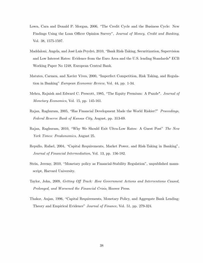
Lown, Cara and Donald P. Morgan, 2006, �The Credit Cycle and the Business Cycle: New
Findings Using the Loan O¢ cer Opinion Survey�, Journal of Money, Credit and Banking,
Vol. 38, 1575-1597.
Maddaloni, Angela, and José Luis Peydró, 2010, �Bank Risk-Taking, Securitization, Supervision
and Low Interest Rates: Evidence from the Euro Area and the U.S. lending Standards" ECB
Working Paper No 1248, European Central Bank.
Matutes, Carmen, and Xavier Vives, 2000, �Imperfect Competition, Risk Taking, and Regula-
tion in Banking�European Economic Review, Vol. 44, pp. 1-34.
Mehra, Rajnish and Edward C. Prescott, 1985, �The Equity Premium: A Puzzle". Journal of
Monetary Economics, Vol. 15, pp. 145-161.
Rajan, Raghuram, 2005, �Has Financial Development Made the World Riskier?� Proceedings,
Federal Reserve Bank of Kansas City, August, pp. 313-69.
Rajan, Raghuram, 2010, �Why We Should Exit Ultra-Low Rates: A Guest Post�The New
York Times: Freakonomics, August 25.
Repullo, Rafael, 2004, �Capital Requirements, Market Power, and Risk-Taking in Banking�,
Journal of Financial Intermediation, Vol. 13, pp. 156-182.
Stein, Jeremy, 2010, �Monetary policy as Financial-Stability Regulation�, unpublished manu-
script, Harvard University.
Taylor, John, 2009, Getting O¤ Track: How Government Actions and Interventions Caused,
Prolonged, and Worsened the Financial Crisis, Hoover Press.
Thakor, Anjan, 1996, �Capital Requirements, Monetary Policy, and Aggregate Bank Lending:
Theory and Empirical Evidence�Journal of Finance, Vol. 51, pp. 279-324.
38