Liquidity and Leverage Hyun Song Shin (Princeton University) and Tobias Adrian (Federal Reserve Bank of New York) Paper presented at the Financial Cycles, Liquidity, and Securitization Conference Hosted by the International Monetary Fund Washington, DC─April 18, 2008 The views expressed in this paper are those of the author(s) only, and the presence of them, or of links to them, on the IMF website does not imply that the IMF, its Executive Board, or its management endorses or shares the views expressed in the paper. F INANCIAL C YCLES ,L IQUIDITY ,AND S ECURITIZATION C ONFERENCE A PRIL 18,2008

Welcome message from author
This document is posted to help you gain knowledge. Please leave a comment to let me know what you think about it! Share it to your friends and learn new things together.
Transcript

Liquidity and Leverage
Hyun Song Shin (Princeton University) and Tobias Adrian (Federal Reserve Bank of New York)
Paper presented at the Financial Cycles, Liquidity, and Securitization Conference Hosted by the International Monetary Fund Washington, DC─April 18, 2008 The views expressed in this paper are those of the author(s) only, and the presence
of them, or of links to them, on the IMF website does not imply that the IMF, its Executive Board, or its management endorses or shares the views expressed in the paper.
FFIINNAANNCCIIAALL CCYYCCLLEESS,, LLIIQQUUIIDDIITTYY,, AANNDD SSEECCUURRIITTIIZZAATTIIOONNCCOONNFFEERREENNCCEE AAPPRRIILL 1188,, 22000088

Liquidity and Leverage�
Tobias Adrian
Federal Reserve Bank of New York
Hyun Song Shin
Princeton University
September 2007
Abstract
In a �nancial system where balance sheets are continuously marked tomarket, asset price changes show up immediately in changes in net worth,and elicit responses from �nancial intermediaries who adjust the size oftheir balance sheets. We document evidence that marked-to-market lever-age is strongly procyclical. Such behavior has aggregate consequences.Changes in aggregate balance sheets for intermediaries forecast changes inrisk appetite in �nancial markets, as measured by the innovations in theVIX index. Aggregate liquidity can be seen as the rate of change of theaggregate balance sheet of the �nancial intermediaries.
�A previous version of this paper was presented at the 6th BIS Annual Conference, \Finan-cial System and Macroeconomic Resilience", 18-19 June 2007 under its former title \Liquidityand Financial Cycles". We thank conference participants at the BIS conference, and seminarparticipants at the Federal Reserve Bank of New York, the Federal Reserve Bank of Chicago,and Princeton University for their comments. The views expressed in this paper are those ofthe authors and do not necessarily represent those of the Federal Reserve Bank of New York orthe Federal Reserve System.
1. Introduction
In a �nancial system where balance sheets are continuously marked to market,
changes in asset prices show up immediately on the balance sheet, and so have
an immediate impact on the net worth of all constituents of the �nancial system.
The net worth of �nancial intermediaries are especially sensitive to uctuations
in asset prices given the highly leveraged nature of such intermediaries' balance
sheets.
Our focus in this paper is on the reactions of the �nancial intermediaries to
changes in their net worth, and the market-wide consequences of such reactions.
If the �nancial intermediaries were passive and do not adjust their balance sheets
to changes in net worth, then leverage would fall when total assets rise. Change
in leverage and change in balance sheet size would then be negatively related.
However, as we will see below, the evidence points to a strongly positive re-
lationship between changes in leverage and changes in balance sheet size. Far
from being passive, the evidence points to �nancial intermediaries adjusting their
balance sheets actively, and doing so in such a way that leverage is high during
booms and low during busts. That is, leverage is procyclical.
Procyclical leverage can be seen as a consequence of the active management of
balance sheets by �nancial intermediaries who respond to changes in prices and
measured risk. For �nancial intermediaries, their models of risk and economic
capital dictate active management of their overall value at risk (VaR) through
adjustments of their balance sheets.
From the point of view of each �nancial intermediary, decision rules that result
in procyclical leverage are readily understandable. However, there are aggregate
consequences of such behavior for the �nancial system as a whole that are not
taken into consideration by an individual �nancial institution. We exhibit evidence
2
that procyclical leverage has spillover e�ects at the aggregate level through shifts
in risk appetite and funding liquidity. In particular, balance sheet uctuations
forecast shifts in risk appetite, as measured by the VIX index.
Our paper has two main objectives. Our �rst objective is to document the
determinants of balance sheet size and leverage for the group of �nancial interme-
diaries (including the major Wall Street investment banks) that operate primarily
through the capital markets. We show that leverage is strongly procyclical for
these intermediaries, and that the margin of adjustment on the balance sheet is
through repos and reverse repos (and other collateralized borrowing and lending).
In turn, procyclical leverage can be attributed to the bank's capital allocation
decision that rests on measured risks ruling at the time. We �nd that the value-
at-risk (VaR) disclosed by the banks is an important determinant of balance sheet
stance, but we also �nd evidence of an additional procyclical element in leverage
that operates over and above that implied by their disclosed value-at-risk.
Our second objective is to pursue the aggregate consequences of such procycli-
cal leverage, and document evidence that expansions and contractions of balance
sheets have important asset pricing consequences through shifts in market-wide
risk appetite. In particular, we show that changes in aggregate intermediary
balance sheet size can forecast innovations in market-wide risk premiums as mea-
sured by the VIX index of implied volatility in the stock market. We see this
as an important empirical �nding. Previous work in asset pricing has shown
that innovations in the VIX index capture key components of asset pricing that
conventional empirical models have been unable to address fully. By being able
to forecast shifts in risk appetite, we hope to inject a new element in thinking
about risk appetite and asset prices. The shift in risk appetite is closely related
to other notions of liquidity, such as the notion of \funding liquidity" used by
3

Brunnermeier and Pedersen (2005b)1. One of our contributions is to explain the
origins of funding liquidity in terms of �nancial intermediary behavior.
Our �ndings also shed light on the concept of \liquidity" as used in common
discourse about �nancial market conditions. In the �nancial press and other mar-
ket commentary, asset price booms are sometimes attributed to \excess liquidity"
in the �nancial system. Financial commentators are fond of using the associated
metaphors, such as the �nancial markets being \awash with liquidity", or liquidity
\sloshing around". However, the precise sense in which \liquidity" is being used
in such contexts is often left unspeci�ed.
Our empirical �ndings suggest that funding liquidity can be understood as the
rate of growth of aggregate balance sheets. When �nancial intermediaries' balance
sheets are generally strong, their leverage is too low. The �nancial intermediaries
hold surplus capital, and they will attempt to �nd ways in which they can employ
their surplus capital. In a loose analogy with manufacturing �rms, we may see
the �nancial system as having \surplus capacity". For such surplus capacity to be
utilized, the intermediaries must expand their balance sheets. On the liabilities
side, they take on more short-term debt. On the asset side, they search for
potential borrowers that they can lend to. Funding liquidity is intimately tied to
how hard the �nancial intermediaries search for borrowers.
The outline of our paper is as follows. We begin with a review of some very ba-
sic balance sheet arithmetic on the relationship between leverage and total assets.
The purpose of this initial exercise is to motivate our empirical investigation of the
balance sheet changes of �nancial intermediaries in section 3. Having outlined the
facts, in section 4, we show that changes in aggregate repo positions of the major
�nancial intermediaries can forecast innovations in the volatility risk-premium,
where the volatility risk premium is de�ned as the di�erence between the VIX
1See also Gromb and Vayanos (2002).
4

index and realized volatility. We conclude with discussions of the implications
of our �ndings for funding liquidity.
2. Some Basic Balance Sheet Arithmetic
What is the relationship between leverage and balance sheet size? We begin with
some very elementary balance sheet arithmetic, so as to focus ideas. Before look-
ing at the evidence for �nancial intermediaries, let us think about the relationship
between balance sheet size and leverage for a household. The household owns a
house �nanced with a mortgage. For concreteness, suppose the house is worth
100, the mortgage value is 90, and so the household has net worth (equity) of 10.
The initial balance sheet then is given by:
Assets Liabilities
100 1090
Leverage is de�ned as the ratio of total assets to equity, hence is 100=10 = 10.
What happens to leverage as total assets uctuate? Denote by A the market
value of total assets and E is the market value of equity. We make the simplifying
assumption that the market value of debt stays roughly constant at 90 for small
shifts in the value of total assets. Total leverage is then
L ' A
A� 90
Leverage is inversely related to total assets. When the price of my house goes up,
my net worth increases, and so my leverage goes down. Figure 2.1 illustrates the
negative relationship between total assets and leverage. Indeed, for households,
the negative relationship between total assets and leverage is clearly borne out
in the aggregate data. Figure 2.2 plots the quarterly changes in total assets to
quarterly changes in leverage as given in the Flow of Funds account for the United
5

Figure 2.1: Leverage for passive investor
States. The data are from 1963 to 2006. The scatter chart shows a strongly
negative relationship, as suggested by Figure 2.1.
Figure 2.2: Total Assets and Leverage of Household.
We can ask the same question for �rms, and we will address this question for
three di�erent types of �rms.
� Non-�nancial �rms
6

� Commercial banks
� Security brokers and dealers (including investment banks).
If a �rm were passive in the face of uctuating asset prices, then leverage would
vary inversely with total assets. However, the evidence points to a more active
management of balance sheets. Figure 2.3 is a scatter chart of the change in
Figure 2.3: Total Assets and Leverage of Non-�nancial, Non-farm Corporates
leverage and change in total assets of non-�nancial, non-farm corporations drawn
from the U.S. ow of funds data (1963 to 2006). The scatter chart shows much
less of a negative pattern, suggesting that companies react to changes in assets by
shifting their stance on leverage.
More notable still is the analogous chart for U.S. commercial banks, again
drawn from the U.S. Flow of Funds accounts. Figure 2.4 is the scatter chart
plotting changes in leverage against changes in total assets for U.S. commercial
banks. A large number of the observations line up along the vertical line that
passes through zero change in leverage. In other words, the data show the outward
signs of commercial banks targeting a �xed leverage ratio.
7

Figure 2.4: Total Assets and Leverage of Commercial Banks
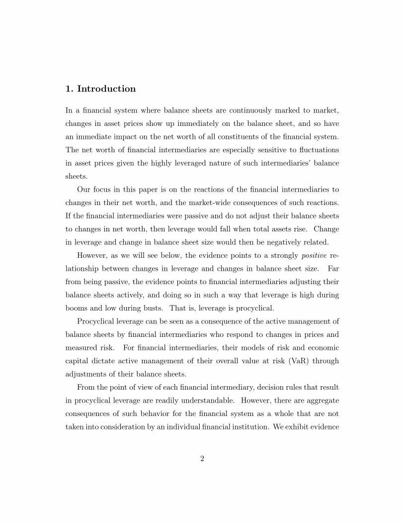
However, even more striking than the scatter chart for commercial banks is that
for security dealers and brokers, that include the major Wall Street investment
banks. Figure 2.5 is the scatter chart for U.S. security dealers and brokers,
again drawn from the Flow of Funds accounts (1963 - 2006). The alignment of
the observations is now the reverse of that for households. There is a strongly
positive relationship between changes in total assets and changes in leverage. In
this sense, leverage is pro-cyclical.
In order to appreciate the aggregate consequences of pro-cyclical leverage, let
us �rst consider the behavior of a �nancial intermediary that manages its balance
sheet actively to as to maintain a constant leverage ratio of 10. Suppose the
initial balance sheet is as follows. The �nancial intermediary holds 100 worth of
securities, and has funded this holding with debt worth 90.
Assets Liabilities
Securities, 100 Equity, 10Debt, 90
8
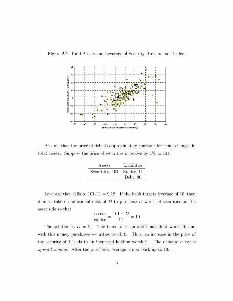
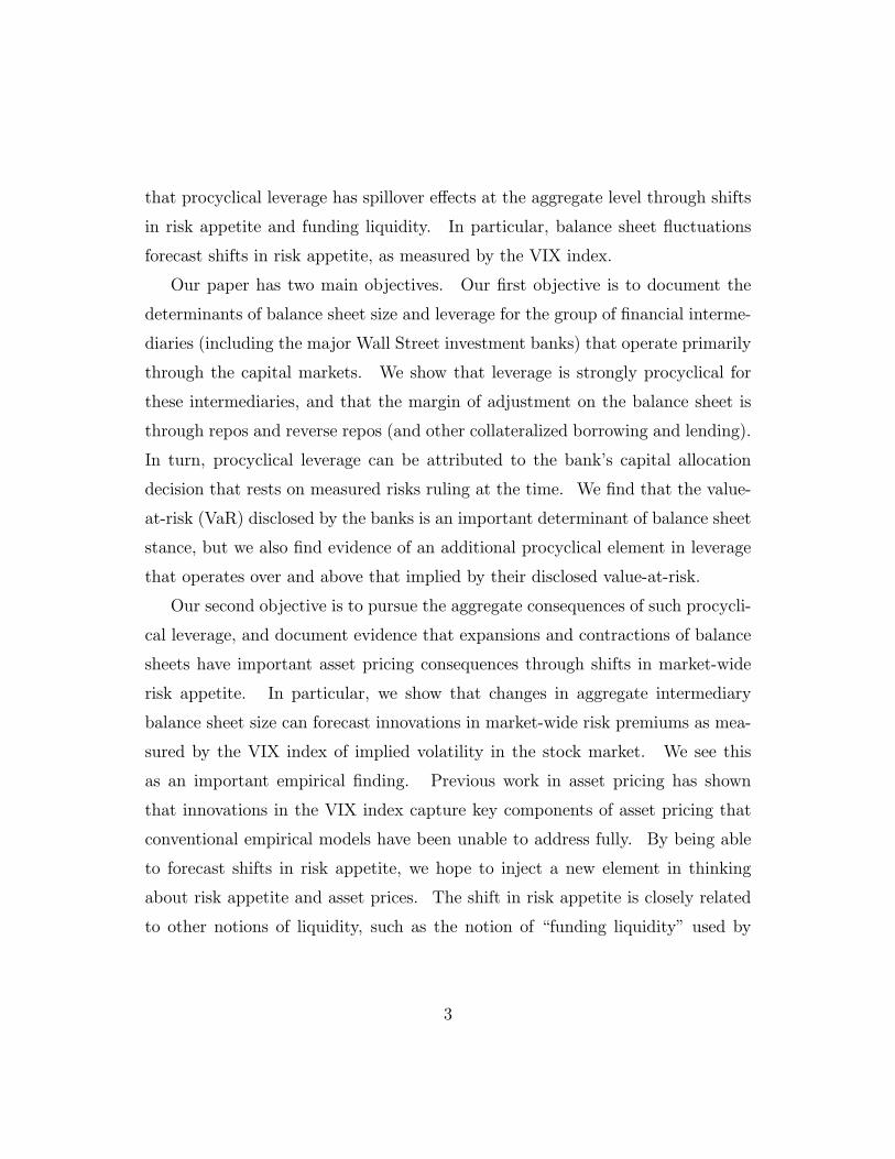
Figure 2.5: Total Assets and Leverage of Security Brokers and Dealers
Assume that the price of debt is approximately constant for small changes in
total assets. Suppose the price of securities increases by 1% to 101.
Assets Liabilities
Securities, 101 Equity, 11Debt, 90
Leverage then falls to 101=11 = 9:18. If the bank targets leverage of 10, then
it must take on additional debt of D to purchase D worth of securities on the
asset side so thatassets
equity=101 +D
11= 10
The solution is D = 9. The bank takes on additional debt worth 9, and
with this money purchases securities worth 9. Thus, an increase in the price of
the security of 1 leads to an increased holding worth 9. The demand curve is
upward-sloping. After the purchase, leverage is now back up to 10.
9

Assets Liabilities
Securities, 110 Equity, 11Debt, 99
The mechanism works in reverse, too. Suppose there is shock to the securities
price so that the value of security holdings falls to 109. On the liabilities side,
it is equity that bears the burden of adjustment, since the value of debt stays
approximately constant.
Assets Liabilities
Securities, 109 Equity, 10Debt, 99
Leverage is now too high (109=10 = 10:9). The bank can adjust down its
leverage by selling securities worth 9, and paying down 9 worth of debt. Thus, a
fall in the price of securities of leads to sales of securities. The supply curve is
downward -sloping. The new balance sheet then looks as follows.
Assets Liabilities
Securities, 100 Equity, 10Debt, 90
The balance sheet is now back to where it started before the price changes.
Leverage is back down to the target level of 10.
Leverage targeting entails upward-sloping demands and downward-sloping sup-
plies. The perverse nature of the demand and supply curves are even stronger
when the leverage of the �nancial intermediary is pro-cyclical - that is, when
leverage is high during booms and low during busts. When the securities price
10

Figure 2.6: Adjustment of Leverage in Booms
goes up, the upward adjustment of leverage entails purchases of securities that
are even larger than that for the case of constant leverage. If, in addition, there
is the possibility of feedback, then the adjustment of leverage and price changes
will reinforce each other in an ampli�cation of the �nancial cycle.
If we hypothesize that greater demand for the asset tends to put upward pres-
sure on its price (a plausible hypothesis, it would seem), then there is the potential
for a feedback e�ect in which stronger balance sheets feed greater demand for the
asset, which in turn raises the asset's price and lead to stronger balance sheets.
Figure 2.6 illustrates the feedback during a boom. The mechanism works exactly
in reverse in downturns. If we hypothesize that greater supply of the asset tends
to put downward pressure on its price, then there is the potential for a feedback
e�ect in which weaker balance sheets lead to greater sales of the asset, which
depresses the asset's price and lead to even weaker balance sheets. Figure 2.7
illustrates the feedback during a downturn.
In section 4, we return to the issue of feedback by exhibiting evidence that
is consistent with the ampli�cation e�ects sketched above. We will see that
11
Figure 2.7: Leverage Adjustment in Downturn
changes in key balance sheet components forecast changes in the VIX index of
implied volatility in the stock market.
3. A First Look at the Evidence
3.1. Investment Bank Balance Sheets
To set the stage for our empirical study, we begin by examining the quarterly
changes in the balance sheets of �ve large investment banks, as listed below in
Table 1. The data are drawn from the Mergent database, which in turn are based
on the regulatory �lings with the U.S. Securities and Exchange Commission (SEC)
on their 10-K and 10-Q forms.
Table 1: Investment Banks
12

Name SampleBear Stearns 1997 Q1 { 2007 Q1
Goldman Sachs 1999 Q2 { 2007 Q1Lehman Brothers 1993 Q2 { 2007 Q1
Merrill Lynch 1991 Q1 { 2007 Q1Morgan Stanley 1997 Q2 { 2007 Q1
Our choice of these �ve banks is motivated by our concern to examine \pure
play" investment banks that are not part of a larger commercial banking group so
as to focus attention on their behavior with respect to the capital markets2. Cit-
igroup reported its investment banking operations separately from its commercial
banking operations until 2004 as \Citigroup Global Markets", and we have data
for the period 1998Q1 to 2004Q4. In some of our charts below, we will report
Citigroup Global Markets for comparison for reference. The stylized balance
sheet of an investment bank is as follows.
Assets Liabilities
Trading assets Short positionsReverse repos ReposOther assets Long term debt
Shareholder equity
On the asset side, traded assets are valued at market prices or are short term
collateralized loans (such as reverse repos) for which the discrepancy between face
value and market value are very small due to the very short term nature of the
loans. On the liabilities side, short positions are at market values, and repos
are very short term borrowing. We will return to a more detailed descriptions
of repos and reverse repos below. Long-term debt is typically a very small frac-
tion of the balance sheet.3 For these reasons, investment banks provide a good
2Hence, we do not include JP Morgan Chase, Credit Suisse, Deutsche Bank, and otherbrokerage operations that are part of a larger commercial bank.
3The balance sheet of Lehman Brothers as of November 2005 shows that short positions arearound a quarter of total assets, and long term debt is an even smaller fraction. Shareholder
13

approximation of the balance sheet that is continuously marked to market, and
hence provide insights into how leverage changes with balance sheet size.
The second reason for our study of investment banks lies in their continuously
increasing signi�cance for the �nancial system.
Figure 3.1:
Figure 3.1 plots the size of securities �rms' balance sheets relative to that
of commercial banks. We also plot the assets under management for hedge
funds, although we should be mindful that \assets under management" refers to
total shareholder equity, rather than the size of the balance sheet. To obtain
total balance sheet size, we should multiply by leverage. Figure 3.1 shows that
when expressed as a proportion of commercial banks' balance sheets, securities
�rms have been increasing their balance sheets at a very rapid rate. Note that
when hedge funds' assets under management is converted to balance sheet size by
multiplying by a conservative leverage factor of 2, the combined balance sheets
equity is around 4% of total assets (implying leverage of around 25). Short-term borrowing interms of repurchase agreements and other collateralized borrowing takes up the remainder.
14
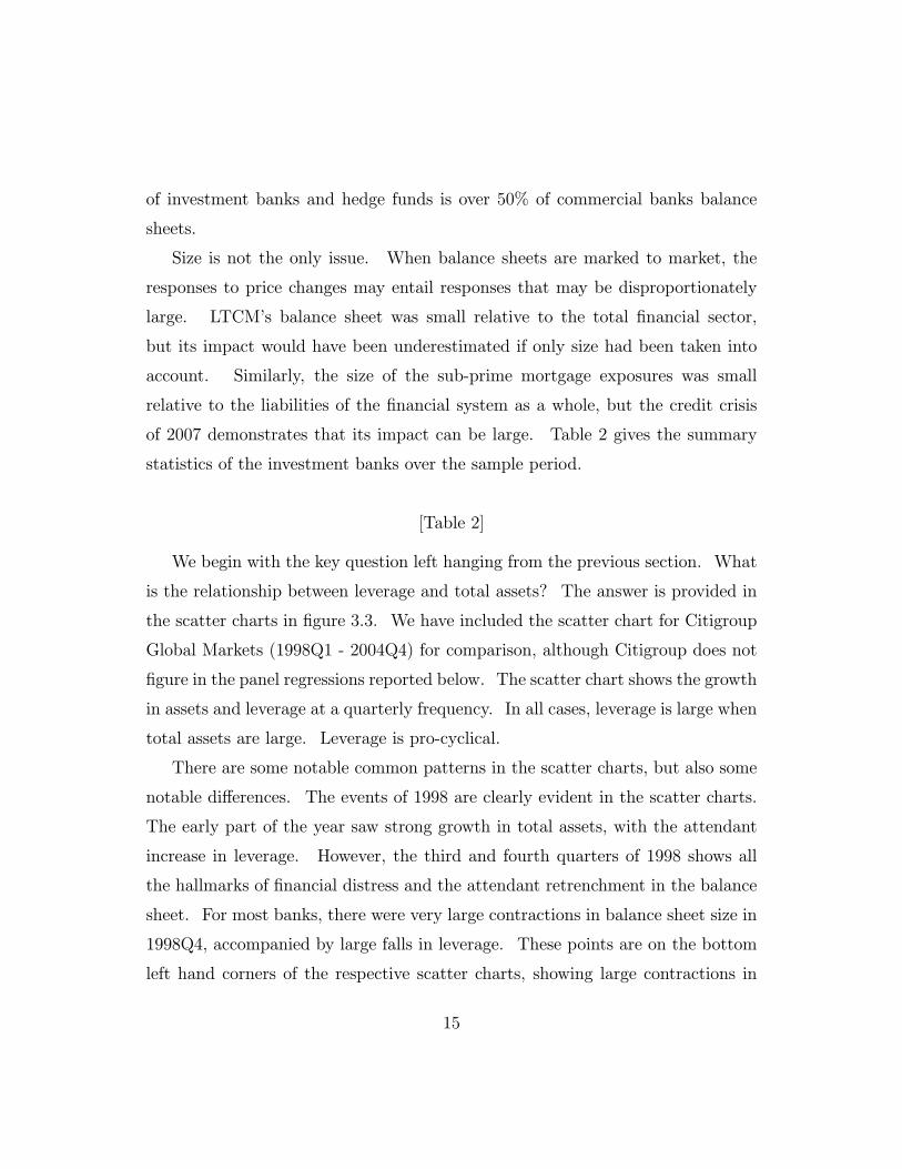
of investment banks and hedge funds is over 50% of commercial banks balance
sheets.
Size is not the only issue. When balance sheets are marked to market, the
responses to price changes may entail responses that may be disproportionately
large. LTCM's balance sheet was small relative to the total �nancial sector,
but its impact would have been underestimated if only size had been taken into
account. Similarly, the size of the sub-prime mortgage exposures was small
relative to the liabilities of the �nancial system as a whole, but the credit crisis
of 2007 demonstrates that its impact can be large. Table 2 gives the summary
statistics of the investment banks over the sample period.
[Table 2]
We begin with the key question left hanging from the previous section. What
is the relationship between leverage and total assets? The answer is provided in
the scatter charts in �gure 3.3. We have included the scatter chart for Citigroup
Global Markets (1998Q1 - 2004Q4) for comparison, although Citigroup does not
�gure in the panel regressions reported below. The scatter chart shows the growth
in assets and leverage at a quarterly frequency. In all cases, leverage is large when
total assets are large. Leverage is pro-cyclical.
There are some notable common patterns in the scatter charts, but also some
notable di�erences. The events of 1998 are clearly evident in the scatter charts.
The early part of the year saw strong growth in total assets, with the attendant
increase in leverage. However, the third and fourth quarters of 1998 shows all
the hallmarks of �nancial distress and the attendant retrenchment in the balance
sheet. For most banks, there were very large contractions in balance sheet size in
1998Q4, accompanied by large falls in leverage. These points are on the bottom
left hand corners of the respective scatter charts, showing large contractions in
15

Figure 3.2:
Figure 3.3:
16
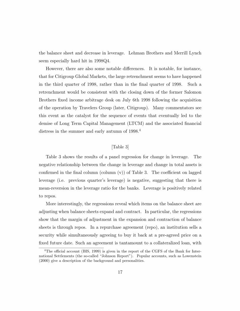
the balance sheet and decrease in leverage. Lehman Brothers and Merrill Lynch
seem especially hard hit in 1998Q4.
However, there are also some notable di�erences. It is notable, for instance,
that for Citigroup Global Markets, the large retrenchment seems to have happened
in the third quarter of 1998, rather than in the �nal quarter of 1998. Such a
retrenchment would be consistent with the closing down of the former Salomon
Brothers �xed income arbitrage desk on July 6th 1998 following the acquisition
of the operation by Travelers Group (later, Citigroup). Many commentators see
this event as the catalyst for the sequence of events that eventually led to the
demise of Long Term Capital Management (LTCM) and the associated �nancial
distress in the summer and early autumn of 1998.4
[Table 3]
Table 3 shows the results of a panel regression for change in leverage. The
negative relationship between the change in leverage and change in total assets is
con�rmed in the �nal column (column (v)) of Table 3. The coe�cient on lagged
leverage (i.e. previous quarter's leverage) is negative, suggesting that there is
mean-reversion in the leverage ratio for the banks. Leverage is positively related
to repos.
More interestingly, the regressions reveal which items on the balance sheet are
adjusting when balance sheets expand and contract. In particular, the regressions
show that the margin of adjustment in the expansion and contraction of balance
sheets is through repos. In a repurchase agreement (repo), an institution sells a
security while simultaneously agreeing to buy it back at a pre-agreed price on a
�xed future date. Such an agreement is tantamount to a collateralized loan, with
4The o�cial account (BIS, 1999) is given in the report of the CGFS of the Bank for Inter-national Settlements (the so-called \Johnson Report"). Popular accounts, such as Lowenstein(2000) give a description of the background and personalities.
17

the interest on the loan being the excess of the repurchase price over the sale price.
From the perspective of the funds lender { the party who buys the security with
the undertaking to re-sell it later { such agreements are called reverse repos. For
the buyer, the transaction is equivalent to granting a loan, secured on collateral.
Repos and reverse repos are important �nancing activities that provide the
funds and securities needed by investment banks to take positions in �nancial
markets. For example, a bank taking a long position by buying a security needs
to deliver funds to the seller when the security is received on settlement day. If
the dealer does not fully �nance the security out of its own capital, then it needs
to borrow funds. The purchased security is typically used as collateral for the
cash borrowing. When the bank sells the security, the sale proceeds can be used
to repay the lender.
Reverse repos are loans made by the investment bank against collateral. The
bank's prime brokerage business vis-�a-vis hedge funds will �gure prominently in
the reverse repo numbers. The scatter chart gives a glimpse into the way in
which changes in leverage are achieved through expansions and contractions in
the collateralized borrowing and lending. We saw in our illustrative section on
the elementary balance sheet arithmetic that when a bank wishes to expand its
balance sheet, it takes on additional debt, and with the proceeds of this borrowing
takes on more assets.
Figure 3.4 plots the change in assets against change in collateralized borrowing.
The positive relationship in the scatter plot con�rms our panel regression �nding
that balance sheet changes are accompanied by changes in short term borrowing.
Figure 3.5 plots the change in repos against the change in reverse repos. A
dealer taking a short position by selling a security it does not own needs to deliver
the security to the buyer on the settlement date. This can be done by borrowing
18

Figure 3.4:
19

Figure 3.5:
20

the needed security, and providing cash or other securities as collateral. When the
dealer closes out the short position by buying the security, the borrowed security
can be returned to the securities lender. The scatter plot in �gure 3.5 suggests
that repos and reverse repos play such a role as counterparts in the balance sheet.
3.2. Value at Risk
Procyclical leverage is not a term that the banks themselves are likely to use in
describing what they do, although this is in fact what they are doing. To get a
better handle on what motivates the banks in their actions, we explore the role of
value at risk (VaR) in explaining the banks' balance sheet decisions.
For a random variable A, the value at risk at con�dence level c relative to
some base level A0 is de�ned as the smallest non-negative number V aR such that
Prob (A < A0 � V aR) � 1� c
For instance, A could be the total marked-to-market assets of the �rm at some
given time horizon. Then the value at risk is the equity capital that the �rm must
hold in order to stay solvent with probability c. Financial intermediaries publish
their value at risk numbers as part of their regulatory �lings, and also regularly
disclose such numbers through their annual reports. Their economic capital is
tied to the overall value at risk of the whole �rm, where the con�dence level is set
at a level high enough to target a given credit rating (typically A or AA).
If �nancial intermediaries adjust their balance sheets to target a ratio of Value-
at-Risk to economic capital, then we may conjecture that their disclosed Value-
at-Risk �gures would be informative in reconstructing their actions. If the bank
maintains capital K to meet total value at risk, then we have
K = �� V aR (3.1)
21
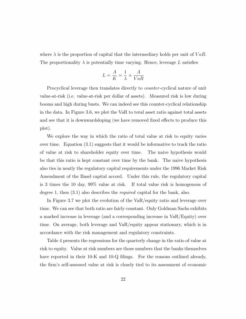
where � is the proportion of capital that the intermediary holds per unit of V aR.
The proportionality � is potentially time varying. Hence, leverage L satis�es
L =A
K=1
�� A
V aR
Procyclical leverage then translates directly to counter -cyclical nature of unit
value-at-risk (i.e. value-at-risk per dollar of assets). Measured risk is low during
booms and high during busts. We can indeed see this counter-cyclical relationship
in the data. In Figure 3.6, we plot the VaR to total asset ratio against total assets
and see that it is downwardsloping (we have removed �xed e�ects to produce this
plot).
We explore the way in which the ratio of total value at risk to equity varies
over time. Equation (3.1) suggests that it would be informative to track the ratio
of value at risk to shareholder equity over time. The naive hypothesis would
be that this ratio is kept constant over time by the bank. The naive hypothesis
also ties in neatly the regulatory capital requirements under the 1996 Market Risk
Amendment of the Basel capital accord. Under this rule, the regulatory capital
is 3 times the 10 day, 99% value at risk. If total value risk is homogenous of
degree 1, then (3.1) also describes the required capital for the bank, also.
In Figure 3.7 we plot the evolution of the VaR/equity ratio and leverage over
time. We can see that both ratio are fairly constant. Only Goldman Sachs exhibits
a marked increase in leverage (and a corresponding increase in VaR/Equity) over
time. On average, both leverage and VaR/equity appear stationary, which is in
accordance with the risk management and regulatory constraints.
Table 4 presents the regressions for the quarterly change in the ratio of value at
risk to equity. Value at risk numbers are those numbers that the banks themselves
have reported in their 10-K and 10-Q �lings. For the reasons outlined already,
the �rm's self-assessed value at risk is closely tied to its assessment of economic
22

Figure 3.6:
23

Figure 3.7:
24

capital, and we would expect behavior to be heavily in uenced by changes in value
at risk.
[Table 4]
We focus on the ratio of value at risk to equity. In the panel regressions, the
lagged value at risk to equity ratio is strongly negative, with coe�cients in the
range of �0:5 to �0:6, suggesting rapid reversion to the mean. We take this as
evidence that the banks use VaR as a cue for how they adjust their balance sheets.
However, the naive hypothesis that banks maintain a �xed ratio of value at risk to
equity does not seem to be supported in the data. Column (ii) of Table 4 suggests
that an increase in the value at risk to equity ratio coincides with periods when the
bank increases its leverage. Value at risk to equity is procyclical, when measured
relative to leverage. However, total assets have a negative sign in column (v). It
appears that value at risk to equity is procyclical, but total assets adjust down
some of the e�ects captured in leverage. The evidence points to an additional,
procyclical risk appetite component to banks' exposures that goes beyond the
simple hypothesis of targeting a normalized value at risk measure.
4. Forecasting Risk Appetite
We now present the main results of our paper. We show the asset pricing conse-
quences of balance sheet expansion and contraction. We have already noted how
the demand and supply responses to price changes can become perverse when
�nancial intermediaries' actions result leverage that co-vary positively with the
�nancial cycle. We exhibit empirical evidence that the waxing and waning of
balance sheets have a direct impact on asset prices through the ease with which
traders, hedge funds and other users of credit can obtain funding for trades.
25

So far, we have used quarterly data drawn either from the balance sheets
of individual �nancial intermediaries or the aggregate balance sheet items from
the Flow of Funds accounts. However, for the purpose of tracking the �nancial
market consequences of balance sheet adjustments, data at a higher frequency is
more likely to be useful. For this reason, we use the weekly data on the primary
dealer repo and reverse repo positions compiled by the Federal Reserve Bank of
New York.
Primary dealers are the dealers with whom the Federal Reserve has an on-going
trading relationship in the course of daily business. The Federal Reserve collects
data that cover transactions, positions, �nancing, and settlement activities in U.S.
Treasury securities, agency debt securities, mortgage-backed securities (MBS),
and corporate debt securities for the primary dealers. The data are used by the Fed
to monitor dealer performance and market conditions, and are also consolidated
and released publicly on the Federal Reserve Bank of New York website5. The
dealers supply market information to the Fed as one of several responsibilities to
maintain their primary dealer designation and hence their trading relationship
with the Fed. It is worth noting that the dealers comprise an important but
limited subset of the overall market. Moreover, dealer reporting entities may not
re ect all positions of the larger organizations. Nevertheless, the primary dealer
data provide a valuable window on the overall market, at a frequency (every week)
that is much higher than the usual quarterly reporting cycle.
Dealers gather information at the close of business each Wednesday, on their
transactions, positions, �nancing, and settlement activities over the previous week.
They report on U.S. Treasury securities, agency debt securities, mortgage backed
securities, and corporate debt securities. Data are then submitted on the following
day (that is, Thursday) via the Federal Reserve System's Internet Electronic Sub-
5www.newyorkfed.org/markets/primarydealers.html
26
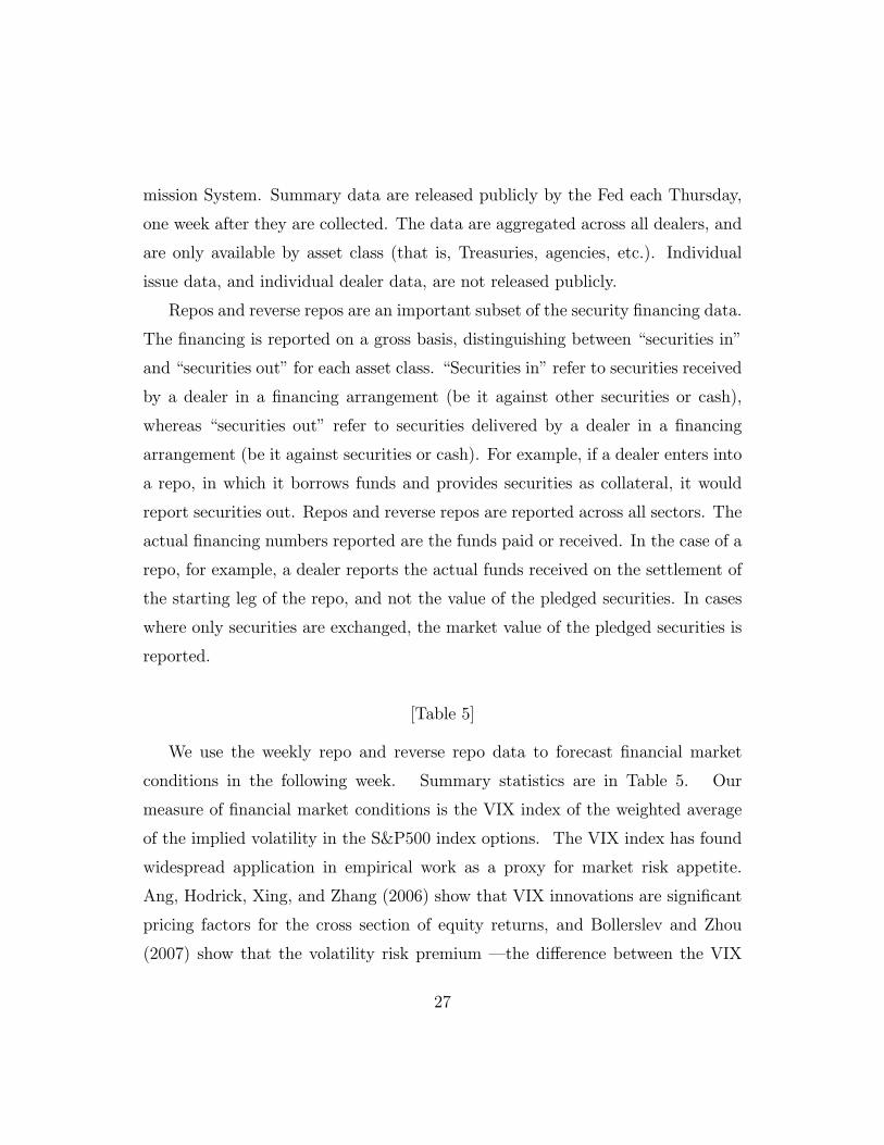
mission System. Summary data are released publicly by the Fed each Thursday,
one week after they are collected. The data are aggregated across all dealers, and
are only available by asset class (that is, Treasuries, agencies, etc.). Individual
issue data, and individual dealer data, are not released publicly.
Repos and reverse repos are an important subset of the security �nancing data.
The �nancing is reported on a gross basis, distinguishing between \securities in"
and \securities out" for each asset class. \Securities in" refer to securities received
by a dealer in a �nancing arrangement (be it against other securities or cash),
whereas \securities out" refer to securities delivered by a dealer in a �nancing
arrangement (be it against securities or cash). For example, if a dealer enters into
a repo, in which it borrows funds and provides securities as collateral, it would
report securities out. Repos and reverse repos are reported across all sectors. The
actual �nancing numbers reported are the funds paid or received. In the case of a
repo, for example, a dealer reports the actual funds received on the settlement of
the starting leg of the repo, and not the value of the pledged securities. In cases
where only securities are exchanged, the market value of the pledged securities is
reported.
[Table 5]
We use the weekly repo and reverse repo data to forecast �nancial market
conditions in the following week. Summary statistics are in Table 5. Our
measure of �nancial market conditions is the VIX index of the weighted average
of the implied volatility in the S&P500 index options. The VIX index has found
widespread application in empirical work as a proxy for market risk appetite.
Ang, Hodrick, Xing, and Zhang (2006) show that VIX innovations are signi�cant
pricing factors for the cross section of equity returns, and Bollerslev and Zhou
(2007) show that the volatility risk premium |the di�erence between the VIX
27

and realized volatility of the S&P500 index | forecasts equity returns better
than other commonly used forecasting variables (such as the P/E ratio or the
term spread).
We use the daily VIX data from the website of the Chicago Board Options
Exchange (www.cboe.com/micro/vix), and compute the S&P500 volatility from
daily data over weekly windows. We compute the volatility risk premium as
the di�erence between implied volatility and realized volatility. This risk pre-
mium is closely linked to the payo� to volatility swaps, which are zero investment
derivatives that return the di�erence between realized future volatility and implied
volatility over the maturity of the swap (see Carr and Wu (2007) for an analysis
of variance and volatility swaps). We then compute averages of the VIX and the
variance risk premium over each week (from the close of Wednesday to the close
of the following Tuesday).
We are able to forecast innovations in the VIX. This can be seen in columns
(ii)-(vi) of Table 6. We report forecasting regressions for VIX changes over the
next week, as well as the Wednesday-Thursday and Wednesday-Friday changes.
All of the forecasting results are signi�cant at the 1% level. The forecasting R2
increases from 8.9% when only the past VIX level is used, column (i) to 11.6%
when Repo changes are included in the forecast. We believe the latter result (the
ability to forecast the innovation in implied volatility) to be a very signi�cant
result. The forecasting result also holds for reverse repos, consistent with the
notion that it is the total size of the balance sheet that matters for aggregate
liquidity.
[Table 6]
In order to gain a better understanding what is determining the forecasting
result, we also run the forecasting regressions for S&P500 volatility and the volatil-
28

Figure 4.1:
ity risk premium (columns vii-x). We see that it is the volatility risk premium
that is being forecast, not actual equity volatility. Adjustments to the size of
�nancial intermediary balance sheets via repos thus forecasts the price of risk of
aggregate volatility, rather than aggregate volatility itself. We provide a graphical
illustration of the forecasting power of repos in Figure 4.1.
We can put forward the following economic rationale for the forecasting re-
gressions presented here. When balance sheets expand through the increased
collateralized lending and borrowing by �nancial intermediaries, the newly re-
29

leased funding resources then chase available assets for purchase. More capital
is deployed in increasing trading positions through the chasing of yield, and the
selling of the \tails", as in the selling of out of the money puts. If the increased
funding for asset purchases result in the generalized increase in prices and risk
appetite in the �nancial system, then the expansion of balance sheets will even-
tually be re ected in the asset price changes in the �nancial system - hence, the
ability of changes in repo positions to forecast future risk appetite.
5. Related Literature
The targeting of leverage seems closely to the bank's attempt to target a particular
credit rating. To the extent that the \passive" credit rating should uctuate
with the �nancial cycle, the fact that a bank's credit rating remains constant
through the cycle suggests that banks manage their leverage actively, so as to shed
exposures during downturns. Kashyap and Stein (2003) draw implications from
such behavior for the pro-cyclical impact of the Basel II bank capital requirements.
To the extent that balance sheets play a central role in our paper, our discussion
here is related to the large literature on the ampli�cation of �nancial shocks. The
literature has distinguished two distinct channels. The �rst is the increased credit
that operates through the borrower's balance sheet, where increased lending comes
from the greater creditworthiness of the borrower (Bernanke and Gertler (1989),
Kiyotaki and Moore (1998, 2001)). The second is the channel that operates
through the banks' balance sheets, either through the liquidity structure of the
banks' balance sheets (Bernanke and Blinder (1988), Kashyap and Stein (2000)),
or the cushioning e�ect of the banks' capital (Van den Heuvel (2002)). Our
discussion is closer to the latter group in that we also focus on the intermediaries'
balance sheets. However, the added insight from our discussions is on the way
that marking to market enhances the role of market prices, and the responses that
30

price changes elicit from intermediaries.
Our results also related to the developing theoretical literature on the role
of liquidity in asset pricing (Gromb and Vayanos (2002), Allen and Gale (2004),
Acharya and Pedersen (2005), Brunnermeier and Pedersen (2005a, 2005b), Morris
and Shin (2004), Acharya, Shin and Yorulmazer (2007a, 2007b)). The common
thread is the relationship between funding conditions and the resulting market
prices of assets. The theme of �nancial distress examined here is also closely
related to the literature on liquidity drains that deal with events such as the stock
market crash of 1987 and the LTCM crisis in the summer of 1998. Gennotte
and Leland (1990) and Geanakoplos (2003) provide analyses that are based on
competitive equilibrium.
The impact of remuneration schemes on the ampli�cations of the �nancial cycle
have been addressed recently by Rajan (2005). The agency problems within a
�nancial institution holds important clues on how we may explain procyclical
behavior. Stein (1997) and Scharfstein and Stein (2000) present analyses of the
capital budgeting problem within banks in the presence of agency problems.
The possibility that a market populated with value at risk (VaR) constrained
traders may have more pronounced uctuations has been examined by Danielsson,
Shin and Zigrand (2004). Mark-to-market accounting may at �rst appear to be
an esoteric question on measurement, but we have seen that it has potentially
important implications for �nancial cycles. Plantin, Sapra and Shin (2005) present
a microeconomic model that compares the performance of marking to market and
historical cost accounting systems.
6. Concluding Remarks
Aggregate liquidity can be understood as the rate of growth of aggregate balance
sheets. When �nancial intermediaries' balance sheets are generally strong, their
31
leverage is too low. The �nancial intermediaries hold surplus capital, and they
will attempt to �nd ways in which they can employ their surplus capital. In a
loose analogy with manufacturing �rms, we may see the �nancial system as having
\surplus capacity". For such surplus capacity to be utilized, the intermediaries
must expand their balance sheets. On the liabilities side, they take on more
short-term debt. On the asset side, they search for potential borrowers that they
can lend to. Aggregate liquidity is intimately tied to how hard the �nancial
intermediaries search for borrowers. In the sub-prime mortgage market in the
United States we have seen that when balance sheets are expanding fast enough,
even borrowers that do not have the means to repay are granted credit - so intense
is the urge to employ surplus capital. The seeds of the subsequent downturn in
the credit cycle are thus sown.
References
Adrian, T. and H. S. Shin (2006) \Money, Liquidity and Financial Cycles" paper
prepared for the Fourth ECB Central Banking Conference, \The Role of Money:
Money and Monetary Policy in the Twenty-First Century", Frankfurt, November
9-10, 2006.
Allen, F. and D. Gale (2004) \Financial Intermediaries and Markets," Economet-
rica 72, 1023-1061.
Acharya, Viral and Lasse Pedersen (2005) \Asset Pricing with Liquidity Risk"
Journal of Financial Economics 77, 375-410.
Ang, A., R. Hodrick, Y Xing, and X. Zhang (2006), \The Cross-Section of Volatil-
ity and Expected Returns," Journal of Finance 61, pp. 259-299.
32

Bank for International Settlements (1999): \A Review of Financial Market Events
in Autumn 1998," CGFS Publication Number 12, Bank for International Settle-
ments, http://www.bis.org/publ/cgfs12.htm.
Bernanke, B. and A. Blinder (1988) \Credit, Money and Aggregate Demand"
American Economic Review, 78, 435-39.
Bernanke, B. and M. Gertler (1989) \Agency Costs, Net Worth, and Business
Fluctuations" American Economic Review, 79, 14 - 31.
Bollerslev, T. and H. Zhou (2007) "Expected Stock Returns and Variance Risk
Premia," Federal Reserve Board Finance and Discussion Series 2007-11.
Brunnermeier, Markus and Lasse Heje Pedersen (2005a) \Predatory Trading",
Journal of Finance, 60, 1825-1863
Brunnermeier, Markus and Lasse Heje Pedersen (2005b) \Market Liquidity and
Funding Liquidity", working paper, Princeton University and NYU Stern School.
Jon Danielsson, Hyun Song Shin and Jean-Pierre Zigrand, (2004) \The Impact
of Risk Regulation on Price Dynamics", Journal of Banking and Finance, 28,
1069-1087
Diamond, Douglas and Raghuram Rajan (2005) \Liquidity Shortages and Banking
Crises" Journal of Finance, 60, pp. 615
Geanakoplos, J. (2003) \Liquidity, Default, and Crashes: Endogenous Contracts
in General Equilibrium" Advances in Economics and Econometrics: Theory and
Applications, Eighth World Conference, Volume II, Cambridge University Press
Gennotte, Gerard and Hayne Leland (1990) \Hedging and Crashes", American
Economic Review, 999{1021.
33

Gromb, Denis and Dimitri Vayanos (2002) \Equilibrium and Welfare in Mar-
kets with Financially Constrained Arbitrageurs", Journal of Financial Economics,
2002, 66, 361-407
Kashyap, A. and J. Stein (2000) \What Do a Million Observations on Banks Say
about the Transmission of Monetary Policy?" American Economic Review, 90,
407-428.
Anil Kashyap and Jeremy Stein, 2003, \Cyclical Implications of the Basel II Cap-
ital Standard", University of Chicago, Graduate School of Business and Harvard
University, http://faculty.chicagogsb.edu/anil.kashyap/research/basel-�nal.pdf
Kiyotaki, N. and J. Moore (1998) \Credit Chains" LSE working paper,
http://econ.lse.ac.uk/sta�/kiyotaki/creditchains.pdf.
Kiyotaki, N. and J. Moore (2001) \Liquidity and Asset Prices" LSE working
paper, http://econ.lse.ac.uk/sta�/kiyotaki/ liquidityandassetprices.pdf.
Carr, P. and Wu, L., (2007) "Variance Risk Premia," Review of Financial Studies,
forthcoming.
Lowenstein, R. (2000) When Genius Failed, Random House, New York.
Plantin, G., H. Sapra and H. S. Shin (2005) \Marking to Market: Panacea or
Pandora's Box" working paper, Princeton University
Rajan, R. (2005) \Has Financial Development Made the World Riskier?" paper
presented at the Federal Reserve Bank of Kansas City Economic Symposium at
Jackson Hole,
http://www.kc.frb.org/publicat/sympos/2005/sym05prg.htm
34

Scharfstein, David and Jeremy Stein (2000) \The Dark Side of Internal Capital
Markets: Divisional Rent-Seeking and Ine�cient Investment" Journal of Finance,
55, 2537-2564.
Stein, Jeremy (1997) \Internal Capital Markets and the Competition for Corpo-
rate Resources" Journal of Finance, 52, 111-133.
Van den Heuvel, S. (2002) \The Bank Capital Channel of Monetary Policy,"
working paper, Wharton School, University of Pennsylvania,
http://�nance.wharton.upenn.edu/~vdheuvel/BCC.pdf
35
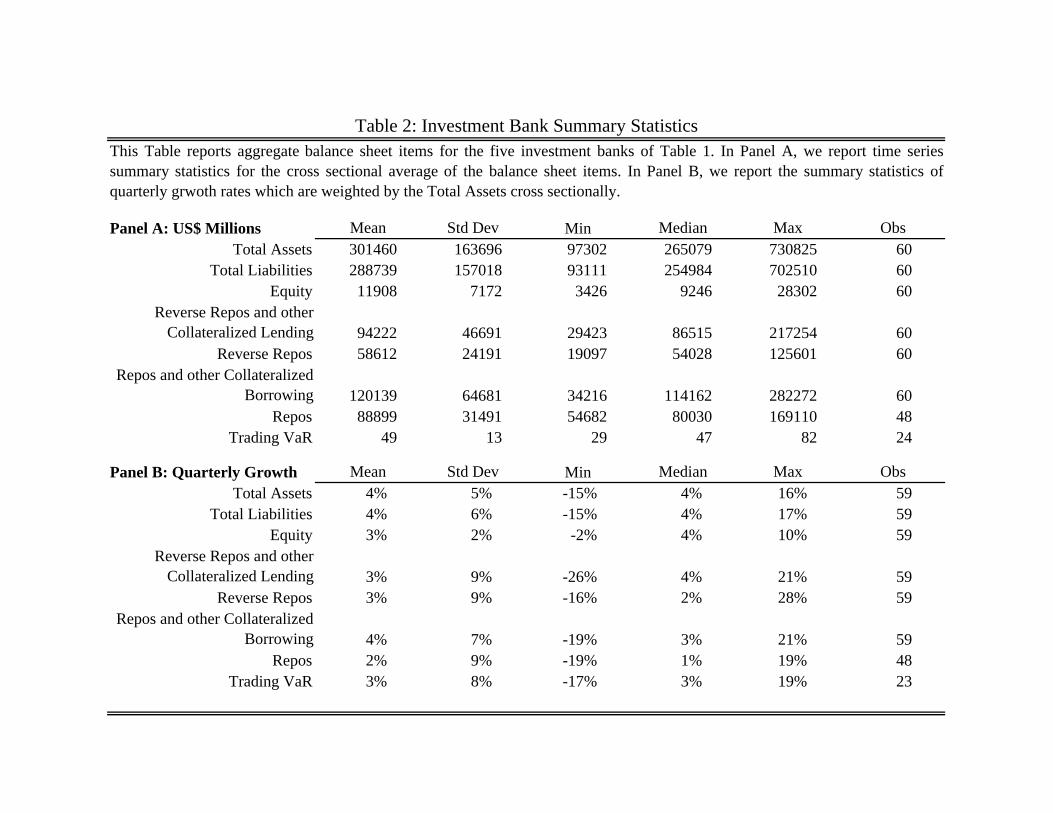
Panel A: US$ Millions Mean Std Dev Min Median Max ObsTotal Assets 301460 163696 97302 265079 730825 60
Total Liabilities 288739 157018 93111 254984 702510 60Equity 11908 7172 3426 9246 28302 60
Reverse Repos and other Collateralized Lending 94222 46691 29423 86515 217254 60
Reverse Repos 58612 24191 19097 54028 125601 60Repos and other Collateralized
Borrowing 120139 64681 34216 114162 282272 60 Repos 88899 31491 54682 80030 169110 48
Trading VaR 49 13 29 47 82 24
Panel B: Quarterly Growth Mean Std Dev Min Median Max ObsTotal Assets 4% 5% -15% 4% 16% 59
Total Liabilities 4% 6% -15% 4% 17% 59Equity 3% 2% -2% 4% 10% 59
Reverse Repos and other Collateralized Lending 3% 9% -26% 4% 21% 59
Reverse Repos 3% 9% -16% 2% 28% 59Repos and other Collateralized
Borrowing 4% 7% -19% 3% 21% 59 Repos 2% 9% -19% 1% 19% 48
Trading VaR 3% 8% -17% 3% 19% 23
This Table reports aggregate balance sheet items for the five investment banks of Table 1. In Panel A, we report time seriessummary statistics for the cross sectional average of the balance sheet items. In Panel B, we report the summary statistics ofquarterly grwoth rates which are weighted by the Total Assets cross sectionally.
Table 2: Investment Bank Summary Statistics
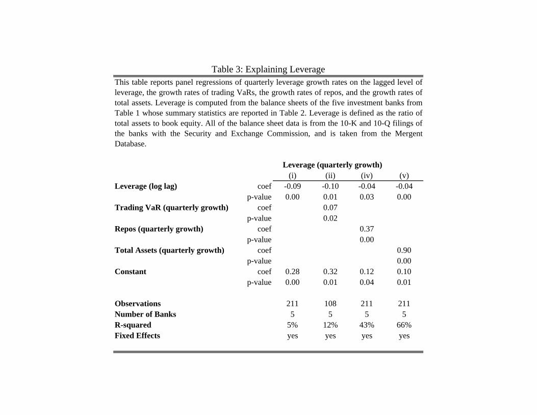
(i) (ii) (iv) (v)Leverage (log lag) coef -0.09 -0.10 -0.04 -0.04
p-value 0.00 0.01 0.03 0.00Trading VaR (quarterly growth) coef 0.07
p-value 0.02Repos (quarterly growth) coef 0.37
p-value 0.00Total Assets (quarterly growth) coef 0.90
p-value 0.00Constant coef 0.28 0.32 0.12 0.10
p-value 0.00 0.01 0.04 0.01
Observations 211 108 211 211Number of Banks 5 5 5 5R-squared 5% 12% 43% 66%Fixed Effects yes yes yes yes
Leverage (quarterly growth)
Table 3: Explaining LeverageThis table reports panel regressions of quarterly leverage growth rates on the lagged level ofleverage, the growth rates of trading VaRs, the growth rates of repos, and the growth rates oftotal assets. Leverage is computed from the balance sheets of the five investment banks fromTable 1 whose summary statistics are reported in Table 2. Leverage is defined as the ratio oftotal assets to book equity. All of the balance sheet data is from the 10-K and 10-Q filings ofthe banks with the Security and Exchange Commission, and is taken from the MergentDatabase.

(i) (ii) (iii) (iv)Trading VaR / Equity (log lag) coef -0.61 -0.56 -0.62 -0.54
p-value 0.00 0.00 0.00 0.00Leverage (quarterly growth) coef 0.91 1.65
p-value 0.00 0.00Total Assets (quarterly growth) coef -0.04 -1.29
p-value 0.90 0.00Constant coef -3.67 -3.32 -3.68 -3.20
p-value 0.00 0.00 0.00 0.00
Observations 107 107 107 107Number of i 5 5 5 5R-squared 33% 39% 33% 44%Fixed Effects yes yes yes yes
Trading VaR / Equity (quarterly growth)
Table 4: Explaining the VaR/Equity RatioThis table reports panel regressions of quarterly growth rates of the ratio of VaR to equity on thelagged level of leverage, the growth rates of trading VaRs, and the growth rates of total assets. Thedata is for the five investment banks from Table 1 whose summary statistics are reported in Table 2.All of the balance sheet data is from the 10-K and 10-Q filings of the banks with the Security andExchange Commission, and is taken from the Mergent Database.

Panel A: US$ Billions Mean Std Dev Min Max ObsReverse Repos and other Collateralized Lending 1712 1010 382 4076 896
Reverse Repos 1655 1008 369 4040 896Repos and other Collateralized Borrowing 1636 961 397 3896 896
Repos 1204 663 332 2636 896Net Repos 451 357 21 1456 896
Panel B: Weekly Growth Mean Std Dev Min Max ObsReverse Repos and other Collateralized Lending 18% 217% -1092% 1360% 895
Reverse Repos 19% 223% -1162% 1344% 895Repos and other Collateralized Borrowing 17% 209% -1097% 1266% 895
Repos 19% 264% -1388% 1471% 895Net Repos 40% 443% -2429% 5356% 895
Table 5: Primary Dealer Financing Summary StatisticsThis Table reports summary statistics of collateralized financing by the Federal Reserve's Primary Dealers from form FR2004 forJanuary 3, 1990 - August 29, 2007.

Volatility Risk PremiumWed-Thur Wed-Fri Thur-Fri
(i) (ii) (iii) (iv) (v) (vi) (vi) (vii) (viii) (ix) (x)Implied Volatility coef -0.12 -0.11 -0.11 -0.12 -0.01 -0.03 -0.03 -0.45 -0.45 0.22 0.21
(lag) p-value 0.00 0.00 0.00 0.00 0.15 0.00 0.00 0.00 0.00 0.00 0.00Repos coef -0.20 -0.05 -0.05 -0.05 0.05 -0.16
(lagged growth) p-value 0.00 0.01 0.04 0.04 0.52 0.03Reverse Repos coef -0.14
(lagged growth) p-value 0.00Net Repos coef -0.06
(lagged growth) p-value 0.00Constant coef 2.16 2.09 2.09 2.14 0.16 0.38 0.38 4.93 4.90 6.23 6.30
p-value 0.00 0.00 0.00 0.00 0.19 0.03 0.03 0.00 0.00 0.00 0.00Observations 903 878 878 878 878 878 878 878 878 878 878R-squared 8.9% 11.6% 10.9% 10.1% 1.1% 1.6% 1.6% 22.8% 22.0% 40.2% 40.9%
One week average Implied Volatility (Change) Volatility (Change)
Table 6: Forecasting VolatilityThis table reports forecasting regressions of VIX implied volatility changes, S&P500 volatility changes, and the volatility risk premium on lagged growthrates of repo, reverse repo, and net repo positions of U.S. Primary Dealers. The VIX is computed from the cross section of S&P500 index option prices bythe Chicago Board of Options Exchange. We compute weekly volatility from S&P500 returns. the volatility risk premium is the difference between theaverage VIX over the week and S&P500 volatility for the same week. Summary statistics of the Primary Dealer financing data are given in Table 5. Thedata is weekly from January 3, 1990 - August 29, 2007. P-values are adjusted for autocorrelation and heteroskedasticity.
Related Documents