Modern Statistical Inference for Classical Statistical Problems
by
Lihua Lei
A dissertation submitted in partial satisfaction of the
requirements for the degree of
Doctor of Philosophy
in
Statistics
in the
Graduate Division
of the
University of California, Berkeley
Committee in charge:
Professor Peter J. Bickel, Co-chairProfessor Michael I. Jordan, Co-chairProfessor Venkatachalam AnantharamAssistant Professor William Fithian
Summer 2019

Modern Statistical Inference for Classical Statistical Problems
Copyright 2019by
Lihua Lei

1
Abstract
Modern Statistical Inference for Classical Statistical Problems
by
Lihua Lei
Doctor of Philosophy in Statistics
University of California, Berkeley
Professor Peter J. Bickel, Co-chair
Professor Michael I. Jordan, Co-chair
This dissertation addresses three classical statistics inference problems with novel ideasand techniques driven by modern statistics. My purpose is to highlight the fact that even themost fundamental problems in statistics are not fully understood and the unexplored partsmay be handled by advances in modern statistics. Pouring new wine into old bottles maygenerate new perspectives and methodologies for more complicated problems. On the otherhand, re-investigating classical problems help us understand the historical development ofstatistics and pick up the scattered pearls forgotten over the course of history.
Chapter 2 discusses my work supervised by Professor Noureddine El Karoui and Pro-fessor Peter J. Bickel on regression M-estimates in moderate dimensions. In this work, weinvestigate the asymptotic distributions of coordinates of regression M-estimates in the mod-erate p/n regime, where the number of covariates p grows proportionally with the samplesize n. Under appropriate regularity conditions, we establish the coordinate-wise asymptoticnormality of regression M-estimates assuming a fixed-design matrix. Our proof is based onthe second-order Poincaré inequality (Chatterjee 2009) and leave-one-out analysis (El Karouiet al. 2011). Some relevant examples are indicated to show that our regularity conditionsare satisfied by a broad class of design matrices. We also show a counterexample, namelythe ANOVA-type design, to emphasize that the technical assumptions are not just artifactsof the proof. Finally, the numerical experiments confirm and complement our theoreticalresults.
Chapter 3 discusses my joint work with Professor Peter J. Bickel on exact inference forlinear models. We propose the cyclic permutation test (CPT) for testing general linearhypotheses for linear models. This test is non-randomized and valid in finite samples withexact type-I error ↵ for arbitrary fixed design matrix and arbitrary exchangeable errors,whenever 1/↵ is an integer and n/p � 1/↵ � 1. The test applies the marginal rank test on1/↵ linear statistics of the outcome vectors where the coefficient vectors are determined bysolving a linear system such that the joint distribution of the linear statistics is invariantto a non-standard cyclic permutation group under the null hypothesis. The power can be

2
further enhanced by solving a secondary non-linear travelling salesman problem, for which thegenetic algorithm can find a reasonably good solution. We show that CPT has comparablepower with existing tests through extensive simulation studies. When testing for a singlecontrast of coefficients, an exact confidence interval can be obtained by inverting the test.Furthermore, we provide a selective yet extensive literature review of the century-long effortson this problem, highlighting the novelty of our test.
Chapter 4 discusses my joint work with Professor Peng Ding on regression adjustmentfor Neyman-Rubin models. Extending R. A. Fisher and D. A. Freedman’s results on theanalysis of covariance, Lin (2013) proposed an ordinary least squares adjusted estimator ofthe average treatment effect in completely randomized experiments. We further study itsstatistical properties under the potential outcomes model in the asymptotic regimes allowingfor a diverging number of covariates. We show that when p >> n1/2, the estimator may havea non-negligible bias and propose a bias-corrected estimator that is asymptotically normalin the regime p = o(n2/3/(log n)1/3). Similar to Lin (2013), our results hold for non-randompotential outcomes and covariates without any model specification. Our analysis requiresnovel analytic tools for sampling without replacement, which complement and potentiallyenrich the theory in other areas such as survey sampling, matrix sketching, and transductivelearning.
i
Contents
Contents i
List of Figures iii
1 Introduction 11.1 Regression M -Estimates in Moderate Dimensions . . . . . . . . . . . . . . . 31.2 Exact Inference for Linear Models . . . . . . . . . . . . . . . . . . . . . . . . 51.3 Regression Adjustment for Neyman-Rubin Models . . . . . . . . . . . . . . . 6
2 Regression M-Estimates in Moderate Dimensions 82.1 Introduction . . . . . . . . . . . . . . . . . . . . . . . . . . . . . . . . . . . . 82.2 More Details on Background . . . . . . . . . . . . . . . . . . . . . . . . . . . 122.3 Main Results . . . . . . . . . . . . . . . . . . . . . . . . . . . . . . . . . . . 162.4 Proof Sketch . . . . . . . . . . . . . . . . . . . . . . . . . . . . . . . . . . . . 272.5 Least-Squares Estimator . . . . . . . . . . . . . . . . . . . . . . . . . . . . . 292.6 Numerical Results . . . . . . . . . . . . . . . . . . . . . . . . . . . . . . . . . 312.7 Conclusion . . . . . . . . . . . . . . . . . . . . . . . . . . . . . . . . . . . . . 35
3 Exact Inference for Linear Models 383.1 Introduction . . . . . . . . . . . . . . . . . . . . . . . . . . . . . . . . . . . . 383.2 Cyclic Permutation Test . . . . . . . . . . . . . . . . . . . . . . . . . . . . . 403.3 Experiments . . . . . . . . . . . . . . . . . . . . . . . . . . . . . . . . . . . . 513.4 1908-2018: A Selective Review of The Century-Long Effort . . . . . . . . . . 563.5 Conclusion and Discussion . . . . . . . . . . . . . . . . . . . . . . . . . . . . 65
4 Regression Adjustment for Neyman-Rubin Models 684.1 Introduction . . . . . . . . . . . . . . . . . . . . . . . . . . . . . . . . . . . . 684.2 Regression Adjustment . . . . . . . . . . . . . . . . . . . . . . . . . . . . . . 714.3 Main Results . . . . . . . . . . . . . . . . . . . . . . . . . . . . . . . . . . . 734.4 Numerical Experiments . . . . . . . . . . . . . . . . . . . . . . . . . . . . . . 794.5 Conclusions and Practical Suggestions . . . . . . . . . . . . . . . . . . . . . 854.6 Technical Lemmas . . . . . . . . . . . . . . . . . . . . . . . . . . . . . . . . 86

ii
4.7 Proofs of The Main Results . . . . . . . . . . . . . . . . . . . . . . . . . . . 88
Bibliography 95
A Appendix for Chapter 2 113A.1 Proof Sketch of Lemma 2.4.5 . . . . . . . . . . . . . . . . . . . . . . . . . . . 113A.2 Proof of Theorem 2.3.1 . . . . . . . . . . . . . . . . . . . . . . . . . . . . . . 118A.3 Proof of Other Results . . . . . . . . . . . . . . . . . . . . . . . . . . . . . . 147A.4 Additional Numerical Experiments . . . . . . . . . . . . . . . . . . . . . . . 168A.5 Miscellaneous . . . . . . . . . . . . . . . . . . . . . . . . . . . . . . . . . . . 169
B Appendix for Chapter 3 173B.1 Complementary Experimental Results . . . . . . . . . . . . . . . . . . . . . . 173
C Appendix for Chapter 4 184C.1 Concentration Inequalities for Sampling Without Replacement . . . . . . . . 184C.2 Mean and Variance of the Sum of Random Rows and Columns of a Matrix . 187C.3 Proofs of the Lemmas in Section 6.2 . . . . . . . . . . . . . . . . . . . . . . . 193C.4 Proof of Proposition 4.3.1 . . . . . . . . . . . . . . . . . . . . . . . . . . . . 196C.5 Proof of Proposition 4.3.2 . . . . . . . . . . . . . . . . . . . . . . . . . . . . 203C.6 Additional Experiments . . . . . . . . . . . . . . . . . . . . . . . . . . . . . 208

iii
List of Figures
2.1 Axpproximation accuracy of p-fixed asymptotics and p/n-fixed asymptotics:each column represents an error distribution; the x-axis represents the ra-tio of the dimension and the sample size and the y-axis represents theKolmogorov-Smirnov statistic; the red solid line corresponds to p-fixed ap-proximation and the blue dashed line corresponds to p/n-fixed approximation. . 14
2.2 Empirical 95% coverage of �1 with = 0.5 (left) and = 0.8 (right) usingHuber1.345 loss. The x-axis corresponds to the sample size, ranging from 100to 800; the y-axis corresponds to the empirical 95% coverage. Each columnrepresents an error distribution and each row represents a type of design. Theorange solid bar corresponds to the case F = Normal; the blue dotted barcorresponds to the case F = t2; the red dashed bar represents the Hadamarddesign. . . . . . . . . . . . . . . . . . . . . . . . . . . . . . . . . . . . . . . . . 34
2.3 Mininum empirical 95% coverage of �1 ⇠ �10 with = 0.5 (left) and =0.8 (right) using Huber1.345 loss. The x-axis corresponds to the sample size,ranging from 100 to 800; the y-axis corresponds to the minimum empirical95% coverage. Each column represents an error distribution and each rowrepresents a type of design. The orange solid bar corresponds to the caseF = Normal; the blue dotted bar corresponds to the case F = t2; the reddashed bar represents the Hadamard design. . . . . . . . . . . . . . . . . . . . 35
2.4 Empirical 95% coverage of �1 ⇠ �10 after Bonferroni correction with = 0.5(left) and = 0.8 (right) using Huber1.345 loss. The x-axis corresponds to thesample size, ranging from 100 to 800; the y-axis corresponds to the empiricaluniform 95% coverage after Bonferroni correction. Each column represents anerror distribution and each row represents a type of design. The orange solidbar corresponds to the case F = Normal; the blue dotted bar corresponds tothe case F = t2; the red dashed bar represents the Hadamard design. . . . . . . 36
3.1 Histograms of O⇤(⇧X) for a realization of a random matrix with i.i.d. Gaus-sian entries. . . . . . . . . . . . . . . . . . . . . . . . . . . . . . . . . . . . . . . 49

iv
3.2 Histograms of O⇤(⇧X) for three matrices as realizations of random one-wayANOVA matrices with exactly one entry in each row at a unifromly randomposition, random matrices with i.i.d. standard normal entries and randommatrices with i.i.d. standard Cauchy entries, respectively. . . . . . . . . . . . . . 50
3.3 Monte-Carlo type-I error for testing a single coordinate with three types ofX’s: (top) realizations of random matrices with i.i.d. standard normal entries;(middle) realizations of random matrices with i.i.d. standard Cauchy entries;(bottom) realizations of random one-way ANOVA design matrices. . . . . . . . 52
3.4 Median power ratio between each variant of CPT and each competing test fortesting a single coordinate with realizations of Gaussian matrices and Gaussianerrors. The black solid line marks the equal power. The missing values in thelast row correspond to infinite ratios. . . . . . . . . . . . . . . . . . . . . . . . . 53
3.5 Median power ratio between each variant of CPT and each competing test fortesting a single coordinate with realizations of Cauchy matrices and Cauchyerrors. The black solid line marks the equal power. The missing values in thelast row correspond to infinite ratios. . . . . . . . . . . . . . . . . . . . . . . . . 54
3.6 Monte-Carlo type-I error for testing five coordinates with three types of X’s:(top) realizations of random matrices with i.i.d. standard normal entries;(middle) realizations of random matrices with i.i.d. standard Cauchy entries;(bottom) realizations of random one-way ANOVA design matrices. . . . . . . . 55
4.1 Simulation with ⇡1 = 0.2. X is a realization of a random matrix with i.i.d.t(2) entries, and e(t) is a realization of a random vector with i.i.d. entriesfrom a distribution corresponding to each column. . . . . . . . . . . . . . . . . 81
4.2 Simulation. X is a realization of a random matrix with i.i.d. t(2) entries, ande(t) is a realization of a random vector with i.i.d. entries from a distributioncorresponding to each column. . . . . . . . . . . . . . . . . . . . . . . . . . . . 82
4.3 Simulation. X is a realization of a random matrix with i.i.d. t(2) entries ande(t) is defined in (4.27): (Left) ⇡1 = 0.2; (Right) ⇡1 = 0.5. . . . . . . . . . . . . 84
4.4 Simulation. Empirical 95% coverage of t-statistics derived from the debiasedestimator with and without trimming the covariate matrix: (Left) ⇡1 = 0.2;(Right) ⇡1 = 0.5. X is a realization of a random matrix with i.i.d. t(2) entriesand e(t) is defined in (4.27). . . . . . . . . . . . . . . . . . . . . . . . . . . . . . 85
A.1 Empirical 95% coverage of �1 with = 0.5 (left) and = 0.8 (right) using L1
loss. The x-axis corresponds to the sample size, ranging from 100 to 800; they-axis corresponds to the empirical 95% coverage. Each column represents anerror distribution and each row represents a type of design. The orange solidbar corresponds to the case F = Normal; the blue dotted bar corresponds tothe case F = t2; the red dashed bar represents the Hadamard design. . . . . . . 169

v
A.2 Mininum empirical 95% coverage of �1 ⇠ �10 with = 0.5 (left) and = 0.8(right) using L1 loss. The x-axis corresponds to the sample size, ranging from100 to 800; the y-axis corresponds to the minimum empirical 95% coverage.Each column represents an error distribution and each row represents a typeof design. The orange solid bar corresponds to the case F = Normal; the bluedotted bar corresponds to the case F = t2; the red dashed bar represents theHadamard design. . . . . . . . . . . . . . . . . . . . . . . . . . . . . . . . . . . 170
A.3 Empirical 95% coverage of �1 ⇠ �10 after Bonferroni correction with = 0.5(left) and = 0.8 (right) using L1 loss. The x-axis corresponds to the samplesize, ranging from 100 to 800; the y-axis corresponds to the empirical uniform95% coverage after Bonferroni correction. Each column represents an errordistribution and each row represents a type of design. The orange solid barcorresponds to the case F = Normal; the blue dotted bar corresponds to thecase F = t2; the red dashed bar represents the Hadamard design. . . . . . . . . 171
B.1 Median power ratio between each variant of CPT and each competing test fortesting a single coordinate with realizations of Gaussian matrices and Cauchyerrors. The black solid line marks the equal power. The missing values in thelast row correspond to infinite ratios. . . . . . . . . . . . . . . . . . . . . . . . . 174
B.2 Median power ratio between each variant of CPT and each competing test fortesting a single coordinate with realizations of Cauchy matrices and Gaussianerrors. The black solid line marks the equal power. The missing values in thelast row correspond to infinite ratios. . . . . . . . . . . . . . . . . . . . . . . . . 175
B.3 Median power ratio between each variant of CPT and each competing testfor testing a single coordinate with realizations of random one-way ANOVAmatrices and Gaussian errors. The black solid line marks the equal power.The missing values in the last row correspond to infinite ratios. . . . . . . . . . 176
B.4 Median power ratio between each variant of CPT and each competing testfor testing a single coordinate with realizations of random one-way ANOVAmatrices and Cauchy errors. The black solid line marks the equal power. Themissing values in the last row correspond to infinite ratios. . . . . . . . . . . . . 177
B.5 Median power ratio between each variant of CPT and each competing test fortesting five coordinates with realizations of Gaussian matrices and Gaussianerrors. The black solid line marks the equal power. The missing values in thelast row correspond to infinite ratios. . . . . . . . . . . . . . . . . . . . . . . . . 178
B.6 Median power ratio between each variant of CPT and each competing testfor testing five coordinates with realizations of Gaussian matrices and Cauchyerrors. The black solid line marks the equal power. The missing values in thelast row correspond to infinite ratios. . . . . . . . . . . . . . . . . . . . . . . . . 179

vi
B.7 Median power ratio between each variant of CPT and each competing testfor testing five coordinates with realizations of Cauchy matrices and Gaussianerrors. The black solid line marks the equal power. The missing values in thelast row correspond to infinite ratios. . . . . . . . . . . . . . . . . . . . . . . . . 180
B.8 Median power ratio between each variant of CPT and each competing testfor testing five coordinates with realizations of Cauchy matrices and Cauchyerrors. The black solid line marks the equal power. The missing values in thelast row correspond to infinite ratios. . . . . . . . . . . . . . . . . . . . . . . . . 181
B.9 Median power ratio between each variant of CPT and each competing test fortesting five coordinates with realizations of random one-way ANOVA matricesand Gaussian errors. The black solid line marks the equal power. The missingvalues in the last row correspond to infinite ratios. . . . . . . . . . . . . . . . . . 182
B.10 Median power ratio between each variant of CPT and each competing test fortesting five coordinates with realizations of random one-way ANOVA matricesand Cauchy errors. The black solid line marks the equal power. The missingvalues in the last row correspond to infinite ratios. . . . . . . . . . . . . . . . . . 183
S1 Simulation. X is a realization of a random matrix with i.i.d. N(0, 1) entriesand e(t) is a realization of a random vector with i.i.d. entries: (Left) ⇡1 = 0.2;(Right) ⇡1 = 0.5. Each column corresponds to a distribution of e(t). . . . . . . 210
S2 Simulation. X is a realization of a random matrix with i.i.d. N(0, 1) entriesand e(t) is defined in (4.27): (Left) ⇡1 = 0.2; (Right) ⇡1 = 0.5. . . . . . . . . . 211
S3 Simulation. X is a realization of a random matrix with i.i.d. t(1) entries ande(t) is a realization of a random vector with i.i.d. entries: (Left) ⇡1 = 0.2;(Right) ⇡1 = 0.5. Each column corresponds to a distribution of e(t). . . . . . . 212
S4 Simulation. X is a realization of a random matrix with i.i.d. t(1) entries ande(t) is defined in (4.27): (Left) ⇡1 = 0.2; (Right) ⇡1 = 0.5. . . . . . . . . . . . . 213
S5 Simulation on Lalonde dataset. e(t) is a realization of a random vector withi.i.d. entries. Each column corresponds to a distribution of e(t). . . . . . . . . . 214
S6 Simulation on Lalonde dataset. e(t) is defined in (4.27). . . . . . . . . . . . . . . 215S7 Simulation on STAR dataset. e(t) is a realization of a random vector with
i.i.d. entries. Each column corresponds to a distribution of e(t). . . . . . . . . . 216S8 Simulation on STAR dataset. e(t) is defined in (4.27). . . . . . . . . . . . . . . . 217

vii
Acknowledgments
First and foremost, I would like to thank my terrific advisors at UC Berkeley, Professor PeterBickel and Professor Michael Jordan, Professor Noureddine El Karoui, Professor WilliamFithian and Professor Peng Ding. Without their tremendous efforts and patience, I wouldnot have been able to work as an academic statistician and contact with a multitude of areas.
My first formal project was supervised by Noureddine and Peter, who impressed me withtheir sagacity, knowledgeability and sharpness. I learned so many deep insights from thediscussion between Noureddine and Peter in our regular weekly meetings for three years.During the period when I doubted if the problem could be solved, Noureddine came upwith the remarkable ideas and techniques which turn out to be the key to the project.Although the final paper is 90-pages long, Noureddine checked the proof line by line andrevised the paper in great details, even in the midst of his sabbatical. Had I not beenadvised by him, I would not have even touched a corner of the iceberg. I deeply appreciatehis tremendous efforts and patience as a remarkable advisor for over three years. Later on Iwas so fortunate to keep working with Peter on other projects beyond pure theory driven byreal-world problems. Peter is the most ingenious statistician I have ever interacted with. Hehas numerous ideas which appear to be abstract and vague at the beginning, but always turnout to work and lead to mind-blowing methodologies. I cannot forget the exciting momentswhen I managed to understand the essence of Peter’s proposals, followed by a big "wow".
Being advised by Mike has been yet another stroke of great fortune. Mike is a "walkingencyclopedia" with a vast knowledge across numerous disciplines, without which I could nothave seen interesting results in different areas. He has always been kind and supportive tome as well as my crazy research ideas. The acronym SCSG, coined by Mike for one of ouralgorithm, is perfect to describe his figure in my mind – Savvy, Creative, Supportive andGentle. Mike also provided an extraordinary research environment, marked by his remarkableweekly group meeting. As a curiosity-driven researcher, it is of great benefit for me to readmaterials on diverse topics, ranging from causal inference to stochastic differential equationsto mechanism designs, together with his wonderful students.
My collaboration with Will started from his fabulous course on selective inference. Beingone of the five enrolled student, my questions filled in almost every one of his lecture. I wasthankful that he did not kick me out of the classroom for being overly challenging and wastotally impressed by the clarity of the answers and the deep insights behind. The course wasso interesting and inspiring that my course project was later turned into my first conferencepublication. In the following collaborations, Will was never falling short of creative ideas oraccurate intuition. His geometry-driven thinking patterns complements my algebra-drivenperspective and greatly improves my research skills.
Peng was my role model in college and I cannot express how excited I were when hechose to join our department as an assistant professor. I must attribute all my researchinterests on causal inference to Peng, who taught me this long-standing topic seriously andthoroughly. Our collaborations were always smooth and efficient due to his kindness andpatience. Beyond his intelligence, I was greatly impressed by his wide knowledge of statistical

viii
history as a junior faculty, which significantly impacted my vision and philosophy of beinga statistician.
My thanks also go to other professors, in particular Professor Venkat Anantharam, whowas extremely kind to be on both my qualifying exam and dissertation committees andprovided helpful comments; Professor Cari Kaufman, who provided guidance and led meinto the Bayesian world in my first semester at Berkeley; Professor Avi Feller, who is oneof the core organizer of the weekly causal reading group which drastically influenced myresearch and motivated a line of joint works; Professor Jasjeet Sekhon, who provided crucialcomments in our joint work; Professor Bin Yu, who taught the excellent 215A course thatexemplified the charm of applied statistics an reshaped my principle of being a good statis-tian; Professor Martin Wainwright, who taught the wonderful 210B course which laid thesolid theoretical foundation for my research; Professor Christopher Paciorek, who providedenormous support for softwares and computation in my research; Professor Elizaveta Levinafrom University of Michigan, who invited me to join the force of her project and providedinstructive and insightful guidance; Professor Guido Imbens from Stanford University, whogave a thought-provoking talk at Berkeley and motivated a joint project. The thanks arealso extended to Professor David Tse, Professor Stefan Wager, Professor Emmanuel Can-dès, Professor Cho-Jui Hsieh, Professor Elizaveth Levina, Professor Xuming He, ProfessorYingying Fan, Professor Fredrik Sävje, Professor Kai Zhang, Professor Chaitra Nagarajaand Professor Linda Zhao for inviting me to give academic talks, which are encouraging asa junior researcher. In addition, I would like to thank my past and current collaboratorsCheng Ju, Yuting Ye, Jianbo Chen, Alexander D’Amour, Aaditya Ramdas, Chiao-Yu Yang,Nhat Ho, Yuchen Wu, Tianxi Li, Sharmodeep Bhattacharyya, Purnamrita Sarkar, MelihElibol, Samuel Horvath, Hongyuan Cao, Zitong Yang, Xingmei Lou and Xiaodong Li.
Next I would to express gratitude to our department and Ph.D. program, which I am veryproud of. I am grateful to all staff, especially La Shana, who is always there helping me withnumerous subtle issues patiently. I am also very thankful to my excellent fellow studentsfrom whom I learn a lot from our academic discussions, in particular Eli Ben-Michael, JosephBorja, Yuansi Chen, Billy Fang, Han Feng, Ryan Giordano, Johnny Hong, Steve Howard,Kenneth Hung, Chi Jin, Sören Künzel, Hongwei Li, Lisa Li, Xiao Li, Tianyi Lin, SujayamSaha, Jake Soloff, Sara Stoudt, Wenpin Tang, Yu Wang, Yuting Wei, Jason Wu, Siqi Wu,Zhiyi You, Da Xu, Renyuan Xu, Chelsea Zhang and Yumeng Zhang. Further I am indebtedto my academic friends outside Berkeley, including but not limited to Yu Bai, Fang Cai, XiChen, Chao Gao, Xinzhou Guo, Zhichao Jiang, Asad Lodhia, Eugene Katsevich, Jason Lee,Song Mei, Nicole Pashley, Zhimei Ren, Feng Ruan, Weijie Su, Qingyun Sun, Pragya Sur,Jingshen Wang, Jingshu Wang, Sheng Xu, Yiqiao Zhong and Qingyuan Zhao.
Finally, I owe the most to my family. My wife Xiaoman Luo always has the magic to bringme peace and confidence when I was stressful, anxious and helpless. Her sense of humor isthe major source of happiness outside my academic life. Meeting and marrying her is mygreatest achievement over the past five years that is more important than any publicationor academic achievement. My parents are always supportive in spite of 6500 miles betweenus. I could not have made any achievement without their unconditional love and support.

1
Chapter 1
Introduction
Inference from data lies at the heart of modern scientific research. Etymologically, the word"inference" means to "carry forward" and can be dated back to late 16th century frommedieval Latin. Despite the solid philosophical and logical foundation, inference is neveran easy task in practice due to uncertainty inherent in data. Statistics, pinoneered in 17thcentury and rapidly developed since early 20th century, is a discipline to generate frameworksand methodologies to understand and handle uncertainty in inference and decision making.Perhaps for this reason, statistical inference grows as a major approach of inference which iswidely adopted in scientific areas.
Recent years have seen a remarkable burst of advances in data collection technology,which have created a dizzying array of exciting application areas for statistical inference.Nowadays phrases like "data science" and "big data" become the new fashion sweeping thesocial media. As a college student majored in statistics, I was deeply attracted by variousfancy concepts and methodologies in modern statistics, marked by the development in 1990ssuch as sparse regression methods, statistical learning methods, social networks, etc.. Butat the same time, my curiosity of classical statistics accrues as I delved further into thearea. "What happened in statistics before 1990s?" – This is a question always haunting myminds. After all, the development over the past century laid the foundation for the successof modern statistics in the era of big data. Although I occasionally learned some classicaltopics from the textbooks, it is not even close to a complete story.
My journey to the old territory of statistics began upon reading Ronald A. Fisher’s1922 article "On the Mathematical Foundation of Theoretical Statistics". In this pioneeringwork, he summarized the purpose of statistical methods as "the reduction of data" and morespecifically, he wrote:
A quantity of data, which usually by its mere bulk is incapable of entering themind, is to be replaced by relatively few quantities which shall adequately rep-resent the whole, or which, in other words, shall contain as much as possible,ideally the whole, of the relevant information contained in the original data.
He further clarified the distinction between a hypothetical population and a sample, between

CHAPTER 1. INTRODUCTION 2
an estimand and an estimator, thereby emphasizing the importance to identify the "sourceof randomness" in statistical inference. Furthermore, he categorized statistical problems intothree types:-
(1) Problems of Specification. These arise in the choice of the mathematical formof the population.(2) Problems of Estimation. These involve the choice of methods of calculatingfrom a sample statistical derivates, or as we shall call them statistics, which aredesigned to estimate the values of the parameters of the hypothetical population.(3) Problems of Distribution. These include discussions of the distribution ofstatistics derived from samples, or in general any functions of quantities whosedistribution is known.
Over the last century, "problems of specification" led to a plethora of statistical models(e.g. linear models, randomization models, time series models, etc.) and identificationstrategies; "problems of estimation" motivated the decision theoretic framework and criteria(e.g. unbiasedness, minimaxity, admissibility, etc.); "problems of distribution" generated theframework of hypothesis testing and the notion of confidence intervals, as well as the solidasymptotic distributional theory.
This remarkable categorization is still valid and quite comprehensive in modern statistics,which is equipped by advanced techniques and refined methodologies but mostly aims athandling the above three tasks. It is therefore valuable for researchers to look back on history,itself being the future of earlier history, to understand how ideas, languages, techniquesand methodologies evolved, as opposed to what they appeared in textbooks written fromhindsight. For instance, had I been a statistician in 1970, I would be more likely thana statistician today to be familiar with Edgeworth expansion, due to the approximationtheory for t-test and F-test in absence of normality (e.g. Bartlett 1935; Wallace 1958). Asa result, it would be more likely for me to understand, or even to discover, the mind-blowing connection between Edgeworth expansion and higher-order accuracy of bootstrap,developed in late 1980s (e.g. Hall 1989, 1992). Similarly, had I been familiar with the earlydevelopment of design-based inference (e.g. Neyman 1923; Welch 1937; Cornfield 1944) andsurvey sampling (e.g. Neyman 1934; Cochran 1977), it would be easier for me to understandthe modern design-based causal inference under the potential outcomes framework (e.g.Freedman 2008b,a; Lin 2013; Bloniarz et al. 2016; Abadie et al. 2017). Those who arefamiliar with classical statistics are more likely able to find and polish the "scattered pearls"that were under-studied or forgotten over the course of history to bring back their brilliance.
On the other hand, the models and the methodologies in classical statistics may not befully understood in spite of the long history. For instance, the linear model is over 100 yearsold but it still inspires new research questions in modern statistics. One remarkable exampleis the breakdown of classical maximum likelihood theory for linear models in moderate di-mensions, where the number of predictors grows linearly with sample size. (Bean et al. 2013)showed that the optimal M-estimator in this regime is no longer the maximum likelihood es-timator but is associated with a complicated loss function determined by a nonlinear system

CHAPTER 1. INTRODUCTION 3
that involves the design properties, the sample size per parameter as well as the error distri-bution (El Karoui et al. 2011). The astonishing finding quickly attracted further attention(e.g. El Karoui 2013, 2015; Donoho and Montanari 2015; Donoho and Montanari 2016; Suret al. 2017; Sur and Candès 2019). Although some earlier works (e.g. Huber 1973a; Bickeland Freedman 1983a) found evidence of non-standard properties of moderate dimensionalregime, the aforementioned line of work was fueled by the advances in random matrix theoryand statistical physics. These works are not purely theoretical pursuit. Instead, they suggestthat the standard softwares may report misleading numbers in many applications even forwell-studied linear models. This is a huge warning for practitioners and will inspire furtherefforts in the future to robustify the built-in algorithms. This inspiring example suggests thetremendous value of investigating classical statistical problems from new perspectives andequipped with advanced techniques.
In my dissertation, I will investigate three classical statistical problems but develop novelideas and techniques to solve them, which I refer to as "modern". Of course, this is anexaggeration since three examples are far too restrictive to show the glamour of modernstatistical inference. Nonetheless, they are epitomes of the elegance and the surprise whenmodern statistical knowledge meets classical statistical problems. In particular, all works inthe dissertation deal with "problems of distribution", in which I found the classical statisticsleave numerous unsolved questions while modern techniques and methodologies have greatpotential to come into play. I sketch the three works in each of the following subsectionsrespectively.
1.1 Regression M-Estimates in Moderate Dimensions
Given a linear model y = X�⇤ + ✏ with outcome vector y 2 Rn, design matrix X 2 Rn⇥p,coefficient vector �⇤ 2 Rp and stochastic errors ✏ 2 Rn, an regression M-estimator is definedas
�(⇢) = argmin�2Rp
nX
i=1
⇢(yi � xT
i�).
M-estimators were proposed by Peter J. Huber in 1960s (Huber 1964) and have been widelystudied in literature (e.g. Relles 1968; Yohai 1972; Huber 1973a; Yohai and Maronna 1979a;Portnoy 1984, 1985; Mammen 1989, 1993). In a nutshell, when the sample size per parametern/p tends to infinity, under some regularity conditions, �(⇢) is consistent in L2 metric andis asymptotically normal in the sense that for any fixed sequence of vectors an 2 Rp,
aTn(�(⇢)� �⇤)paTn⌃nan
=) N(0, 1), where ⌃ = Cov(�(⇢)). (1.1)
However, the story completely changes in the moderate dimensional regime, where p/n ! 2 (0, 1). In moderate dimensions, the sample size per parameter is bounded away frominfinity and thus there are insufficient samples for estimating every coefficient accurately. For

CHAPTER 1. INTRODUCTION 4
least-squares estimators, Huber (1973a) proved that (1.1) is impossible for every sequenceof an’s in moderate dimensions. For general M-estimators with particular random designs,El Karoui et al. (2011) showed the inconsistency of �(⇢) in L2 metric and characterized thelimiting L2 risk as the solution of a delicate nonlinear system involving , the distributionof X and the distribution of errors. On the other hand, Bean et al. (2013) proved (1.1) withGaussian design matrices for any fixed sequence of an’s in moderate dimensions. This isnot contradicted to Huber (1973a) as the latter assumes a fixed design and thus the claim(1.1) only involves the randomness from ✏, while Bean et al. (2013)’s result also considersthe randomness of design matrices which brings more regularity.
These works inspired a line of studies that extended the results to general settings (ElKaroui 2013, 2015; Donoho and Montanari 2015; Donoho and Montanari 2016; Sur et al.2017; Sur and Candès 2019). However, most of them focused on special random designs, suchas Gaussian matrices or random matrices with elliptically distributed rows. Furthermore,their central research question is to determine the limiting risk of �(⇢). Although someattempts have been made to the "problem of distribution", the results are based on Gaussiandesigns (Bean et al. 2013; Donoho and Montanari 2016; Sur et al. 2017; Sur and Candès2019), with a few exceptions on more general random designs (El Karoui 2015, 2018), andsome of them are about the "bulk distribution" of all coefficients which is less interpretableto practitioners. No distributional result was established previously for general M-estimatorswith fixed designs in moderate dimensions.
In this chapter, we ask a classical question: what is the asymptotic distribution of agiven coordinate of �(⇢) in moderate dimensions assuming a fixed design. This question issurprisingly hard to answer than it appears to be, mainly due to the fundamental difficultylying in the moderate dimensional regime. Unlike the low dimensional regime , in which theestimator has asymptotically linearity and thus the Linderberg-Feller-type central limit the-orem can be applied to prove the asymptotic normality, the Taylor-expansion-type argumentdoes not carry over to in moderate dimensional regime because there is only bounded num-ber of samples on average for each parameter. Instead, we apply the second-order Poincaréinequality (Chatterjee 2009) that can be regarded as a generalization of classical centrallimit theorem to nonlinear transformation of independent random variables. In addition,we replace the Taylor-expansion-type argument by a more involved leave-one-out argumentthat generalizes El Karoui (2013)’s techniques to fixed-designs. In summary, we prove thefollowing result.
Theorem 1.1.1 (Informal Version). Under appropriate conditions on the design matrix X,the distribution of ✏ and the loss function ⇢, as p/n ! 2 (0, 1), while n ! 1,
max1jp
dTV
0
@L
0
@ �j(⇢)� �⇤jq
Var(�j(⇢))
1
A , N(0, 1)
1
A = o(1)
where dTV(·, ·) is the total variation distance and L(·) denotes the law.

CHAPTER 1. INTRODUCTION 5
We also show a counterexample, namely the one-way analysis of variance problem withnon-normal errors, to emphasize that our technical assumptions are not an artifact of theproof but essential to some extent, thereby revealing the non-standard property of the mod-erate dimensional regime.
This chapter is adapted from my joint work with Professor Noureddine El Karoui andProfessor Peter J. Bickel. The paper was published on Probability Theory and Related Fieldson December, 2018 (Lei et al. 2018). The idea was originated from Noureddine El Karouiand Peter Bickel as an extension of their earlier works (El Karoui et al. 2011; El Karoui 2013;Bean et al. 2013; El Karoui 2015, 2018). Noureddine El Karoui and Peter Bickel providedjoint advising on this work, with joint meetings of the three of us weekly over the course oftwo years or so.
1.2 Exact Inference for Linear Models
Chapter 2 highlights the difficulty in deriving asymptotics even for a single coordinate witha bounded number of samples per parameter. However, the moderate dimensional regime isquite common in practice as n/p 50 in many applications. This may suggest the frangibilityof classical asymptotic theory which back up the numbers reported (e.g. p-values, confidenceintervals) by standard softwares. It is thus natural to ask if there exists a robust inferentialprocedure in moderate dimensional regime.
In this chapter, we consider the problem of testing a linear hypothesis, under the linearmodels studied in Chapter 2, in the form H0 : RT�⇤ = 0, where R 2 Rp⇥r is a matrix withfull collumn rank. In particular, if R = (1, 0, . . . , 0)T , then it is equivalent to testing for thefirst coordinate. Suppose we can find a valid test, then a confidence interval can be obtainedfor �⇤
1by inverting the test, thereby yielding a valid inferential procedure, at least for a single
coordinate.Testing linear hypotheses for linear models is a century-long problem started in 1920s
and various qualitatively different strategies have been proposed to tackle this problem,including normal theory based methods (e.g. Fisher 1922; Fisher 1924; Snedecor 1934),permutation-based methods (e.g. Pitman 1937b,a; Pitman 1938), rank-based methods (e.g.Friedman 1937; Theil 1950a), tests based on regression R-estimates (e.g. Hájek 1962), M-estimates (e.g. Huber 1973a), L-estimates (e.g. Bickel 1973), resampling-based methods (e.g.Freedman 1981) and other methods (e.g. Brown and Mood 1951; Daniels 1954; Hartigan1970; Meinshausen 2015). However, as opposed to the location problems and analysis ofvariance problems, none of those tests are provably robust to the moderate dimensionalregime under reasonably general assumptions.
In this chapter, we propose the cyclic permutation test (CPT), which is an exact non-randomized test for a given confidence level ↵, for arbitrary fixed design matrices and arbi-trary exchangeable errors, provided that 1/↵ is an integer and n/p � 1/↵� 1. For instance,CPT only requires n/p � 19 when ↵ = 0.05 and thus works in moderate dimensions. No-tably, exact tests for general linear hypotheses are rare over the past century and they

CHAPTER 1. INTRODUCTION 6
are all restricted to linear models with stringent assumptions. By contrast, CPT is exactin finite samples and almost assumption-free except for the exchangeability of errors. Weshow that CPT has comparable power with existing tests, which may not have guaranteeof validity, through extensive numerical experiments. The existence of such a non-standard,assumption-free but powerful test suggests that "problem of distribution" may be tackledby new techniques.
This chapter is adapted from my joint work with Professor Peter J. Bickel. The preprintwas posted on ArXiv on July, 2019 (Lei and Bickel 2019).
1.3 Regression Adjustment for Neyman-Rubin Models
In 1923, Jerzy Neyman proposed a model for analyzing agonormic trials in his master thesis(Neyman 1923), which is later known as randomization model (Scheffé 1959), and quicklybecame one of the main pillar in analysis of experimental data (e.g. Kempthorne 1952) andsurvey sampling (e.g. Cochran 1977). Notably, Donald B. Rubin introduced this modelinto causal inference, established the framework of potential outcomes and generalized it toobservational studies in his seminal work (Rubin 1974). For this reason, the randomizationmodel is also called Neyman-Rubin model in causal inference literature.
Neyman-Rubin model is fundamentally different from linear models. The linear modelwith fixed designs, marked by analysis of variance, assumes that the treatment assignmentis fixed and the outcome is a random variable centered at a linear function of treatmentvariables. By contrast, the Neyman-Rubin model assumes that the treatment assignment israndom with a known distribution and the outcome is a fixed number given the treatmentvalues. To be concrete, given a binary treatment T with observed outcomes Y obs, the linearmodel assumes Y obs
i= ↵ + �Ti + ✏i where ✏i is a random variable while the Neyman-Rubin
model assumes Y obs
i= Yi(1)T+Yi(0)(1�T ) where Yi(1) and Yi(0), called potential outcomes,
are two numbers that are either fixed or independent of the treatment Ti. Clearly, the sourceof randomness is different based on two models. Inference based on linear models wasusually classified as model-based inference, because it uses the functional relation betweenthe outcome and the treatment, while inference based on Neyman-Rubin models was usuallyclassified as design-based inference; see Särndal et al. (e.g. 1978) and Abadie et al. (2017). Onthe other hand, the inferential targets are usually different for two models. For linear models,the effect of the treatment can be easily defined as �, the coefficient of the treatment variable;for Neyman-Rubin models, the effect of the treatment is usually defined as the average ofindividual effects, i.e. 1/n
Pn
i=1(Yi(1) � Yi(0)). The former can be regarded as a special
case of the latter if we treat Yi(1) = ↵ + � + ✏i and Yi(0) = ↵ + ✏i. Inference based onNeyman-Rubin model is more general, though at the cost of the knowledge of the treatmentassignment mechanism. Nonetheless, for experimental data, it comes as a free lunch asthe assignment mechanism is known by design. Therefore the Neyman-Rubin model is arobust alternative to the linear model in cases where the researcher has more knowledge ofthe treatment assignment mechanism than that of the functional relation between observed

CHAPTER 1. INTRODUCTION 7
outcomes and the treatment.In many applications, baseline covariates are usually collected together with the treatment
assignment (e.g. demographic information of experimental subjects). A natural approach isto run a linear regression of the observed outcome on the treatment assignment and the co-variates and estimate the effect of the treatment by the corresponding regression coefficient.The fundamental difference between two models does not prevent us from evaluating thisprocedure, which is clearly valid for a linear model, under the Neyman-Rubin model. How-ever, Freedman (2008b) criticized this approach, showing that it may be less efficient thanthe naive difference-in-means estimator which completely ignores covariates. He pointed outthat the failure is driven by the different sources of randomness between linear models andNeyman-Rubin models. Interestingly, Lin (2013) proposed a simple remedy by adding theinteraction terms between the treatment and the covariates into the regression and showedthat this estimator is never less efficient than the difference-in-means estimator in the asymp-totic regime where the number of covariates p stays fixed while the sample size n tends toinfinity.
Based on my experience in linear models as mentioned in the last two subsections, theasymptotics based on fixed-p regime may not be reliable. For a real problem with n = 1000and p = 50, is the asymptotic result a plausible approximation? Bloniarz et al. (2016) tookthe first in a high-dimensional setting where p >> n. However they considered a differentestimator and assumed an approximately sparse relation between the potential outcomesand the covariates. Instead, we consider Lin (2013) in a more classical setting where noassumption is imposed on the potential outcomes except some regularity conditions involvingthe finite sample moments. Specifically, for completely randomized experiments, we showthat Lin (2013)’s estimator is consistent when log p ! 0 and asymptotically normal whenp ! 0 under mild moment conditions, where is the maximum leverage score of thecovariate matrix. In the favorable case where leverage scores are all close together, hisestimator is consistent when p = o(n/ log n) and is asymptotically normal when p = o(n1/2).Beyond this regime, we find that the estimator may have a non-negligible bias. For thisreason, we propose a bias-corrected estimator that is consistent when log p ! 0 and isasymptotically normal, with the same variance in the fixed-p regime, when 2p log p ! 0.In the favorable case, the latter condition reduces to p = o(n2/3/(log n)1/3). Our analysesrequire novel concentration inequalities for sampling without replacement, driven by modernprobability theory.
This chapter is adapted from my joint work with Professor Peng Ding. The preprint wasposted on ArXiv on June, 2018 (Lei and Ding 2018).

8
Chapter 2
Regression M -Estimates in ModerateDimensions
2.1 Introduction
High-dimensional statistics has a long history (Huber 1973a; Wachter 1976, 1978) withconsiderable renewed interest over the last two decades. In many applications, the researchercollects data which can be represented as a matrix, called a design matrix and denoted byX 2 Rn⇥p, as well as a response vector y 2 Rn and aims to study the connection betweenX and y. The linear model is among the most popular models as a starting point of dataanalysis in various fields. A linear model assumes that
y = X�⇤ + ✏, (2.1)
where �⇤ 2 Rp is the coefficient vector which measures the marginal contribution of eachpredictor and ✏ is a random vector which captures the unobserved errors.
The aim of this chapter is to provide valid inferential results for features of �⇤. Forexample, a researcher might be interested in testing whether a given predictor has a negligibleeffect on the response, or equivalently whether �⇤
j= 0 for some j. Similarly, linear contrasts
of �⇤ such as �⇤1� �⇤
2might be of interest in the case of the group comparison problem in
which the first two predictors represent the same feature but are collected from two differentgroups.
An M-estimator, defined as
�(⇢) = argmin�2Rp
1
n
nX
i=1
⇢(yi � xT
i�) (2.2)
where ⇢ denotes a loss function, is among the most popular estimators used in practice(Relles 1968; Huber 1973a). In particular, if ⇢(x) = 1
2x2, �(⇢) is the famous Least Square
Estimator (LSE). We intend to explore the distribution of �(⇢), based on which we canachieve the inferential goals mentioned above.

CHAPTER 2. REGRESSION M -ESTIMATES IN MODERATE DIMENSIONS 9
The most well-studied approach is the asymptotic analysis, which assumes that the scaleof the problem grows to infinity and use the limiting result as an approximation. In regressionproblems, the scale parameter of a problem is the sample size n and the number of predictorsp. The classical approach is to fix p and let n grow to infinity. It has been shown (Relles1968; Yohai 1972; Huber 1972; Huber 1973a) that �(⇢) is consistent in terms of L2 norm andasymptotically normal in this regime. The asymptotic variance can be then approximatedby the bootstrap (Bickel and Freedman 1981). Later on, the studies are extended to theregime in which both n and p grow to infinity but p/n converges to 0 (Yohai and Maronna1979b; Portnoy 1984, 1985, 1986, 1987; Mammen 1989). The consistency, in terms of the L2
norm, the asymptotic normality and the validity of the bootstrap still hold in this regime.Based on these results, we can construct a 95% confidence interval for �0j simply as �j(⇢)±1.96
qdVar(�j(⇢)) where dVar(�j(⇢)) is calculated by bootstrap. Similarly we can calculate
p-values for the hypothesis testing procedure.We ask whether the inferential results developed under the low-dimensional assumptions
and the software built on top of them can be relied on for moderate and high-dimensionalanalysis? Concretely, if in a study n = 50 and p = 40, can the software built upon theassumption that p/n ' 0 be relied on when p/n = .8? Results in random matrix theory(Marčenko and Pastur 1967) already offer an answer in the negative side for many PCA-related questions in multivariate statistics. The case of regression is more subtle: For instancefor least-squares, standard degrees of freedom adjustments effectively take care of manydimensionality-related problems. But this nice property does not extend to more generalregression M-estimates.
Once these questions are raised, it becomes very natural to analyze the behavior andperformance of statistical methods in the regime where p/n is fixed. Indeed, it will help usto keep track of the inherent statistical difficulty of the problem when assessing the variabilityof our estimates. In other words, we assume in this chapter that p/n ! > 0 while letn grows to infinity. Due to identifiability issues, it is impossible to make inference on �⇤
if p > n without further structural or distributional assumptions. We discuss this point indetails in Section 2.2.3. Thus we consider the regime where p/n ! 2 (0, 1). We call itthe moderate p/n regime. This regime is also the natural regime in random matrix theory(Marčenko and Pastur 1967; Wachter 1978; Johnstone 2001; Bai and Silverstein 2010). Ithas been shown that the asymptotic results derived in this regime sometimes provide anextremely accurate approximation to finite sample distributions of estimators at least incertain cases (Johnstone 2001) where n and p are both small.
2.1.1 Qualitatively Different Behavior of Moderate p/n Regime
First, �(⇢) is no longer consistent in terms of L2 norm and the risk Ek�(⇢) � �⇤k2 tendsto a non-vanishing quantity determined by , the loss function ⇢ and the error distributionthrough a complicated system of non-linear equations (El Karoui et al. 2011; El Karoui 2013,2015; Bean et al. 2012). This L2-inconsistency prohibits the use of standard perturbation-

CHAPTER 2. REGRESSION M -ESTIMATES IN MODERATE DIMENSIONS 10
analytic techniques to assess the behavior of the estimator. It also leads to qualitatively dif-ferent behaviors for the residuals in moderate dimensions; in contrast to the low-dimensionalcase, they cannot be relied on to give accurate information about the distribution of theerrors. However, this seemingly negative result does not exclude the possibility of inferencesince �(⇢) is still consistent in terms of L2+⌫ norms for any ⌫ > 0 and in particular in L1norm. Thus, we can at least hope to perform inference on each coordinate.
Second, classical optimality results do not hold in this regime. In the regime p/n ! 0,the maximum likelihood estimator is shown to be optimal (Huber 1964; Huber 1972; Bickeland Doksum 2015). In other words, if the error distribution is known then the M-estimatorassociated with the loss ⇢(·) = � log f✏(·) is asymptotically efficient, provided the design isof appropriate type, where f✏(·) is the density of entries of ✏. However, in the moderate p/nregime, it has been shown that the optimal loss is no longer the log-likehood but an otherfunction with a complicated but explicit form (Bean et al. 2013), at least for certain designs.The suboptimality of maximum likelihood estimators suggests that classical techniques failto provide valid intuition in the moderate p/n regime.
Third, the joint asymptotic normality of �(⇢), as a p-dimensional random vector, maybe violated for a fixed design matrix X. This has been proved for least-squares by Huber(1973a) in his pioneering work. For general M-estimators, this negative result is a simpleconsequence of the results of El Karoui et al. (2011): They exhibit an ANOVA design (seebelow) where even marginal fluctuations are not Gaussian. By contrast, for random design,they show that �(⇢) is jointly asymptotically normal when the design matrix is ellipticalwith general covariance by using the non-asymptotic stochastic representation for �(⇢) aswell as elementary properties of vectors uniformly distributed on the uniform sphere in Rp;See section 2.2.3 of El Karoui et al. (2011) or the supplementary material of Bean et al.(2013) for details. This does not contradict Huber (1973a)’s negative result in that it takesthe randomness from both X and ✏ into account while Huber (1973a)’s result only takes therandomness from ✏ into account. Later, El Karoui (2015) shows that each coordinate of �(⇢)is asymptotically normal for a broader class of random designs. This is also an elementaryconsequence of the analysis in El Karoui (2013). However, to the best of our knowledge,beyond the ANOVA situation mentioned above, there are no distributional results for fixeddesign matrices. This is the topic of this chapter.
Last but not least, bootstrap inference fails in this moderate-dimensional regime. Thishas been shown by Bickel and Freedman (1983b) for least-squares and residual bootstrap intheir influential work. Recently, El Karoui and Purdom (2015) studied the results to generalM-estimators and showed that all commonly used bootstrapping schemes, including pairs-bootstrap, residual bootstrap and jackknife, fail to provide a consistent variance estimatorand hence valid inferential statements. These latter results even apply to the marginaldistributions of the coordinates of �(⇢). Moreover, there is no simple, design independent,modification to achieve consistency (El Karoui and Purdom 2015).

CHAPTER 2. REGRESSION M -ESTIMATES IN MODERATE DIMENSIONS 11
2.1.2 Our ContributionsIn summary, the behavior of the estimators we consider in this chapter is completely differentin the moderate p/n regime from its counterpart in the low-dimensional regime. As discussedin the next section, moving one step further in the moderate p/n regime is interestingfrom both the practical and theoretical perspectives. Our main contribution is to establishcoordinate-wise asymptotic normality of �(⇢) for certain fixed design matrices X in thisregime under technical assumptions. The following theorem informally states our mainresult.
Theorem 2.1.1 (Informal Version of Theorem 2.3.1 in Section 2.3). Under appropriateconditions on the design matrix X, the distribution of ✏ and the loss function ⇢, as p/n ! 2 (0, 1), while n ! 1,
max1jp
dTV
0
@L
0
@ �j(⇢)� E�j(⇢)qVar(�j(⇢))
1
A , N(0, 1)
1
A = o(1)
where dTV(·, ·) is the total variation distance and L(·) denotes the law.
It is worth mentioning that the above result can be extended to finite dimensional linearcontrasts of �. For instance, one might be interested in making inference on �⇤
1� �⇤
2in the
problems involving the group comparison. The above result can be extended to give theasymptotic normality of �1 � �2.
Besides the main result, we have several other contributions. First, we use a new approachto establish asymptotic normality. Our main technique is based on the second-order Poincaréinequality (SOPI), developed by Chatterjee (2009) to derive, among many other results,the fluctuation behavior of linear spectral statistics of random matrices. In contrast toclassical approaches such as the Lindeberg-Feller central limit theorem, the second-orderPoincaré inequality is capable of dealing with nonlinear and potentially implicit functions ofindependent random variables. Moreover, we use different expansions for �(⇢) and residualsbased on double leave-one-out ideas introduced in El Karoui et al. (2011), in contrast tothe classical perturbation-analytic expansions. See aforementioned paper and follow-ups.An informal interpretation of the results of Chatterjee (2009) is that if the Hessian of thenonlinear function of random variables under consideration is sufficiently small, this functionacts almost linearly and hence a standard central limit theorem holds.
Second, to the best of our knowledge this is the first inferential result for fixed (nonANOVA-like) design in the moderate p/n regime. Fixed designs arise naturally from an ex-perimental design or a conditional inference perspective. That is, inference is ideally carriedout without assuming randomness in predictors; see Section 2.2.2 for more details. We clarifythe regularity conditions for coordinate-wise asymptotic normality of �(⇢) explicitly, whichare checkable for LSE and also checkable for general M-estimators if the error distribution isknown. We also prove that these conditions are satisfied with by a broad class of designs.

CHAPTER 2. REGRESSION M -ESTIMATES IN MODERATE DIMENSIONS 12
The ANOVA-like design described in Section 2.3.3 exhibits a situation where the distri-bution of �j(⇢) is not going to be asymptotically normal. As such the results of Theorem2.3.1 below are somewhat surprising.
For complete inference, we need both the asymptotic normality and the asymptotic biasand variance. Under suitable symmetry conditions on the loss function and the error dis-tribution, it can be shown that �(⇢) is unbiased (see Section 2.3.2 for details) and thus itis left to derive the asymptotic variance. As discussed at the end of Section 2.1.1, classicalapproaches, e.g. bootstrap, fail in this regime. For least-squares, classical results continue tohold and we discuss it in section 2.5 for the sake of completeness. However, for M-estimators,there is no closed-form result. We briefly touch upon the variance estimation in Section 2.3.4.The derivation for general situations is beyond the scope of this chapter and left to the futureresearch.
2.1.3 OutlineThe rest of the chapter is organized as follows: In Section 2.2, we clarify details which arementioned in the current section. In Section 2.3, we state the main result (Theorem 2.3.1)formally and explain the technical assumptions. Then we show several examples of randomdesigns which satisfy the assumptions with high probability. In Section 4, we introduceour main technical tool, second-order Poincaré inequality (Chatterjee 2009), and apply iton M-estimators as the first step to prove Theorem 2.3.1. Since the rest of the proof ofTheorem 2.3.1 is complicated and lengthy, we illustrate the main ideas in Appendix A.1.The rigorous proof is left to Appendix A.2. In Section 2.5, we provide reminders about thetheory of least-squares estimation for the sake of completeness, by taking advantage of itsexplicit form. In Section 2.6, we display the numerical results. The proof of other results arestated in Appendix A.3 and more numerical experiments are presented in Appendix A.4.
2.2 More Details on Background
2.2.1 Moderate p/n Regime: a more informative type ofasymptotics?
In Section 2.1, we mentioned that the ratio p/n measures the difficulty of statistical inference.The moderate p/n regime provides an approximation of finite sample properties with thedifficulties fixed at the same level as the original problem. Intuitively, this regime shouldcapture more variation in finite sample problems and provide a more accurate approximation.We will illustrate this via simulation.
Consider a study involving 50 participants and 40 variables; we can either use the asymp-totics in which p is fixed to be 40, n grows to infinity or p/n is fixed to be 0.8, and n grows toinfinity to perform approximate inference. Current software rely on low-dimensional asymp-totics for inferential tasks, but there is no evidence that they yield more accurate inferential
CHAPTER 2. REGRESSION M -ESTIMATES IN MODERATE DIMENSIONS 13
statements than the ones we would have obtained using moderate dimensional asymptotics.In fact, numerical evidence (Johnstone 2001; El Karoui et al. 2013; Bean et al. 2013) showthat the reverse is true.
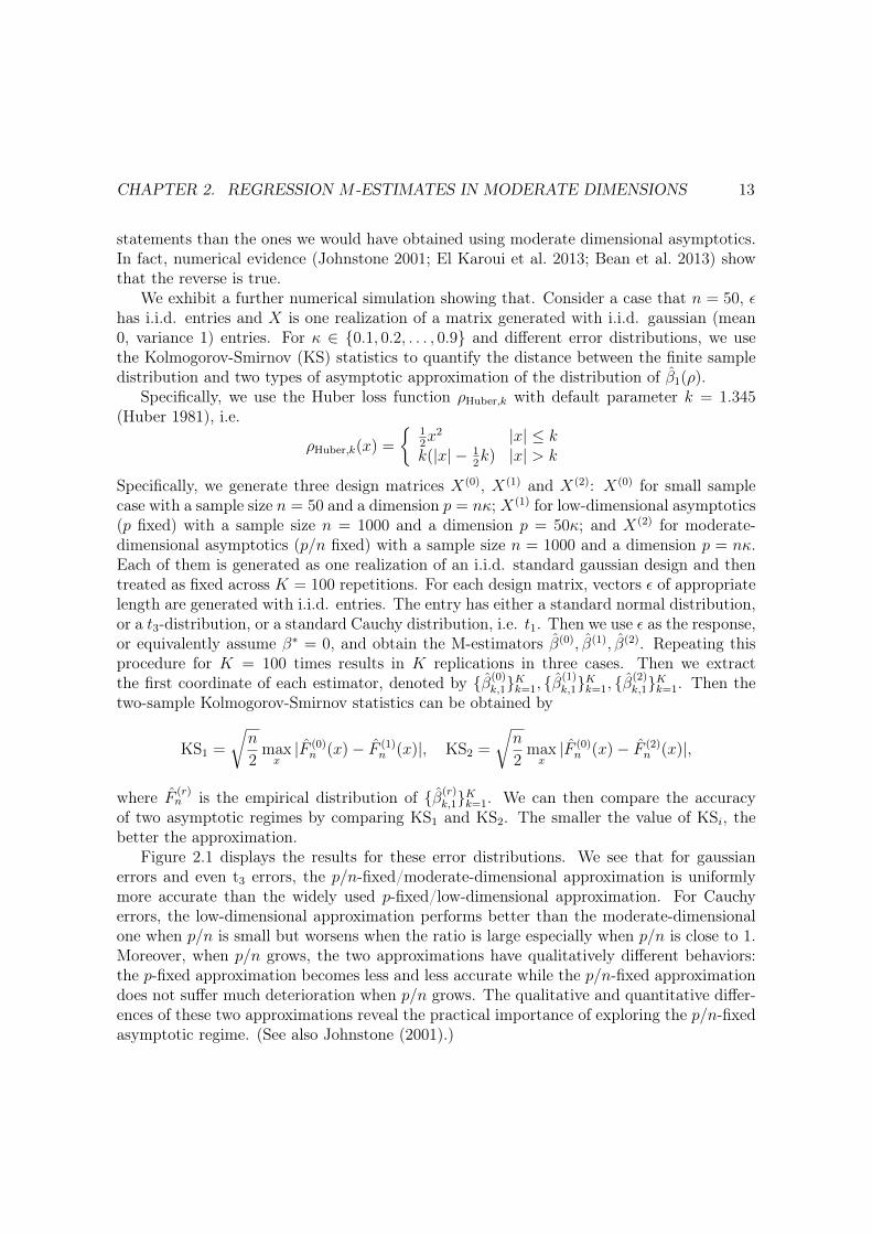
We exhibit a further numerical simulation showing that. Consider a case that n = 50, ✏has i.i.d. entries and X is one realization of a matrix generated with i.i.d. gaussian (mean0, variance 1) entries. For 2 {0.1, 0.2, . . . , 0.9} and different error distributions, we usethe Kolmogorov-Smirnov (KS) statistics to quantify the distance between the finite sampledistribution and two types of asymptotic approximation of the distribution of �1(⇢).
Specifically, we use the Huber loss function ⇢Huber,k with default parameter k = 1.345(Huber 1981), i.e.
⇢Huber,k(x) =
⇢1
2x2 |x| k
k(|x|� 1
2k) |x| > k
Specifically, we generate three design matrices X(0), X(1) and X(2): X(0) for small samplecase with a sample size n = 50 and a dimension p = n; X(1) for low-dimensional asymptotics(p fixed) with a sample size n = 1000 and a dimension p = 50; and X(2) for moderate-dimensional asymptotics (p/n fixed) with a sample size n = 1000 and a dimension p = n.Each of them is generated as one realization of an i.i.d. standard gaussian design and thentreated as fixed across K = 100 repetitions. For each design matrix, vectors ✏ of appropriatelength are generated with i.i.d. entries. The entry has either a standard normal distribution,or a t3-distribution, or a standard Cauchy distribution, i.e. t1. Then we use ✏ as the response,or equivalently assume �⇤ = 0, and obtain the M-estimators �(0), �(1), �(2). Repeating thisprocedure for K = 100 times results in K replications in three cases. Then we extractthe first coordinate of each estimator, denoted by {�(0)
k,1}Kk=1
, {�(1)
k,1}Kk=1
, {�(2)
k,1}Kk=1
. Then thetwo-sample Kolmogorov-Smirnov statistics can be obtained by
KS1 =
rn
2max
x
|F (0)
n(x)� F (1)
n(x)|, KS2 =
rn
2max
x
|F (0)
n(x)� F (2)
n(x)|,
where F (r)
n is the empirical distribution of {�(r)
k,1}Kk=1
. We can then compare the accuracyof two asymptotic regimes by comparing KS1 and KS2. The smaller the value of KSi, thebetter the approximation.
Figure 2.1 displays the results for these error distributions. We see that for gaussianerrors and even t3 errors, the p/n-fixed/moderate-dimensional approximation is uniformlymore accurate than the widely used p-fixed/low-dimensional approximation. For Cauchyerrors, the low-dimensional approximation performs better than the moderate-dimensionalone when p/n is small but worsens when the ratio is large especially when p/n is close to 1.Moreover, when p/n grows, the two approximations have qualitatively different behaviors:the p-fixed approximation becomes less and less accurate while the p/n-fixed approximationdoes not suffer much deterioration when p/n grows. The qualitative and quantitative differ-ences of these two approximations reveal the practical importance of exploring the p/n-fixedasymptotic regime. (See also Johnstone (2001).)

CHAPTER 2. REGRESSION M -ESTIMATES IN MODERATE DIMENSIONS 14
normal t(3) cauchy
● ●
● ● ● ●
●
●
●
● ●●
●●
●● ●
●
●
●● ●
●●
●
● ●
● ● ●●
●●
●
●
●
●
●
●
●
●
●
●●
●
●●
●
●●
●●
●
●0.25
0.30
0.35
0.40
0.45
0.50
0.25 0.50 0.75 0.25 0.50 0.75 0.25 0.50 0.75kappa
Kolm
ogor
ov−S
mirn
ov S
tatis
tics
Asym. Regime ● ●p fixed p/n fixed
Distance between the small sample and large sample distribution
Figure 2.1: Axpproximation accuracy of p-fixed asymptotics and p/n-fixed asymptotics: eachcolumn represents an error distribution; the x-axis represents the ratio of the dimensionand the sample size and the y-axis represents the Kolmogorov-Smirnov statistic; the red solidline corresponds to p-fixed approximation and the blue dashed line corresponds to p/n-fixedapproximation.
2.2.2 Random vs fixed design?As discussed in Section 2.1.1, assuming a fixed design or a random design could lead toqualitatively different inferential results.
In the random design setting, X is considered as being generated from a super population.For example, the rows of X can be regarded as an i.i.d. sample from a distribution known,or partially known, to the researcher. In situations where one uses techniques such as cross-validation (Stone 1974), pairs bootstrap in regression (Efron and Efron 1982) or samplesplitting (Wasserman and Roeder 2009), the researcher effectively assumes exchangeabilityof the data (xT
i, yi)ni=1
. Naturally, this is only compatible with an assumption of randomdesign. Given the extremely widespread use of these techniques in contemporary machinelearning and statistics, one could argue that the random design setting is the one under whichmost of modern statistics is carried out, especially for prediction problems. Furthermore,working under a random design assumption forces the researcher to take into account twosources of randomness as opposed to only one in the fixed design case. Hence working undera random design assumption should yield conservative confidence intervals for �⇤
j.
In other words, in settings where the researcher collects data without control over thevalues of the predictors, the random design assumption is arguably the more natural one ofthe two.
However, it has now been understood for almost a decade that common random designassumptions in high-dimension (e.g. xi = ⌃1/2zi where zi,j’s are i.i.d with mean 0 andvariance 1 and a few moments and ⌃ “well behaved") suffer from considerable geometriclimitations, which have substantial impacts on the performance of the estimators considered

CHAPTER 2. REGRESSION M -ESTIMATES IN MODERATE DIMENSIONS 15
in this chapter (El Karoui et al. 2011). As such, confidence statements derived from thatkind of analysis can be relied on only after performing a few graphical tests on the data (seeEl Karoui (2010)). These geometric limitations are simple consequences of the concentrationof measure phenomenon (Ledoux 2001).
On the other hand, in the fixed design setting, X is considered a fixed matrix. In thiscase, the inference only takes the randomness of ✏ into consideration. This perspective ispopular in several situations. The first one is the experimental design. The goal is to studythe effect of a set of factors, which can be controlled by the experimenter, on the response. Incontrast to the observational study, the experimenter can design the experimental conditionahead of time based on the inference target. For instance, a one-way ANOVA design encodesthe covariates into binary variables (see Section 2.3.3 for details) and it is fixed prior to theexperiment. Other examples include two-way ANOVA designs, factorial designs, Latin-square designs, etc. (Scheffe 1999).
Another situation which is concerned with fixed design is the survey sampling wherethe inference is carried out conditioning on the data (Cochran 1977). Generally, in orderto avoid unrealistic assumptions, making inference conditioning on the design matrix Xis necessary. Suppose the linear model (2.1) is true and identifiable (see Section 2.2.3 fordetails), then all information of �⇤ is contained in the conditional distribution L(y|X) andhence the information in the marginal distribution L(X) is redundant. The conditionalinference framework is more robust to the data generating procedure due to the irrelevanceof L(X).
Also, results based on fixed design assumptions may be preferable from a theoretical pointof view in the sense that they could potentially be used to establish corresponding resultsfor certain classes of random designs. Specifically, given a marginal distribution L(X), oneonly has to prove that X satisfies the assumptions for fixed design with high probability.
In conclusion, fixed and random design assumptions play complementary roles in moder-ate dimensional settings. We focus on the least understood of the two, the fixed design case,in this chapter.
2.2.3 Modeling and Identification of ParametersThe problem of identifiability is especially important in the fixed design case. Define �⇤(⇢)in the population as
�⇤(⇢) = argmin�2Rp
1
n
nX
i=1
E⇢(yi � xT
i�). (2.3)
One may ask whether �⇤(⇢) = �⇤ regardless of ⇢ in the fixed design case. We providean affirmative answer in the following proposition by assuming that ✏i has a symmetricdistribution around 0 and ⇢ is even.

CHAPTER 2. REGRESSION M -ESTIMATES IN MODERATE DIMENSIONS 16
Proposition 2.2.1. Suppose X has a full column rank and ✏id= �✏i for all i. Further
assume ⇢ is an even convex function such that for any i = 1, 2, . . . and ↵ 6= 0,1
2(E⇢(✏i � ↵) + E⇢(✏i + ↵)) > E⇢(✏i). (2.4)
Then �⇤(⇢) = �⇤ regardless of the choice of ⇢.
The proof is left to Appendix A.3. It is worth mentioning that Proposition 2.2.1 onlyrequires the marginals of ✏ to be symmetric but does not impose any constraint on thedependence structure of ✏. Further, if ⇢ is strongly convex, then for all ↵ 6= 0,
1
2(⇢(x� ↵) + ⇢(x+ ↵)) > ⇢(x).
As a consequence, the condition (2.4) is satisfied provided that ✏i is non-zero with positiveprobability.
If ✏ is asymmetric, we may still be able to identify �⇤ if ✏i are i.i.d. random variables.In contrast to the last case, we should incorporate an intercept term as a shift towards thecentroid of ⇢. More precisely, we define ↵⇤(⇢) and �⇤(⇢) as
(↵⇤(⇢), �⇤(⇢)) = argmin↵2R,�2Rp
1
n
nX
i=1
E⇢(yi � ↵� xT
i�).
Proposition 2.2.2. Suppose (1, X) is of full column rank and ✏i are i.i.d. such that E⇢(✏1�↵) as a function of ↵ has a unique minimizer ↵(⇢). Then �⇤(⇢) is uniquely defined with�⇤(⇢) = �⇤ and ↵⇤(⇢) = ↵(⇢).
The proof is left to Appendix A.3. For example, let ⇢(z) = |z|. Then the minimizer ofE⇢(✏1 � a) is a median of ✏1, and is unique if ✏1 has a positive density. It is worth pointingout that incorporating an intercept term is essential for identifying �⇤. For instance, in theleast-square case, �⇤(⇢) no longer equals to �⇤ if E✏i 6= 0. Proposition 2.2.2 entails thatthe intercept term guarantees �⇤(⇢) = �⇤, although the intercept term itself depends on thechoice of ⇢ unless more conditions are imposed.
If ✏i’s are neither symmetric nor i.i.d., then �⇤ cannot be identified by the previouscriteria because �⇤(⇢) depends on ⇢. Nonetheless, from a modeling perspective, it is popularand reasonable to assume that ✏i’s are symmetric or i.i.d. in many situations. Therefore,Proposition 2.2.1 and Proposition 2.2.2 justify the use of M-estimators in those cases and M-estimators derived from different loss functions can be compared because they are estimatingthe same parameter.
2.3 Main Results
2.3.1 Notation and AssumptionsLet xT
i2 R1⇥p denote the i-th row of X and Xj 2 Rn⇥1 denote the j-th column of X.
Throughout the chapter we will denote by Xij 2 R the (i, j)-th entry of X, by X[j] 2 Rn⇥(p�1)

CHAPTER 2. REGRESSION M -ESTIMATES IN MODERATE DIMENSIONS 17
the design matrix X after removing the j-th column, and by xT
i,[j]2 R1⇥(p�1) the vector xT
i
after removing j-th entry. The M-estimator �(⇢) associated with the loss function ⇢ is definedas
�(⇢) = argmin�2Rp
1
n
nX
k=1
⇢(yk � xT
k�) = argmin
�2Rp
1
n
nX
k=1
⇢(✏k � xT
k(� � �⇤)) (2.5)
We define = ⇢0 to be the first derivative of ⇢. We will write �(⇢) simply � when noconfusion can arise.
When the original design matrix X does not contain an intercept term, we can simplyreplace X by (1, X) and augment � into a (p + 1)-dimensional vector (↵, �T )T . Althoughbeing a special case, we will discuss the question of intercept in Section 2.3.2 due to itsimportant role in practice.
Equivariance and reduction to the null caseNotice that our target quantity �j�E�jp
Var(�j)is invariant to the choice of �⇤, provided that �⇤ is
identifiable as discussed in Section 2.2.3, we can assume �⇤ = 0 without loss of generality.In this case, we assume in particular that the design matrix X has full column rank. Thenyk = ✏k and
� = argmin�2Rp
1
n
nX
k=1
⇢(✏k � xT
k�).
Similarly we define the leave-j-th-predictor-out version as
�[j] = argmin�2Rp�1
1
n
nX
k=1
⇢(✏k � xT
k,[j]�).
Based on these notations we define the full residuals Rk as
Rk = ✏k � xT
k�, k = 1, 2, . . . , n
and the leave-j-th-predictor-out residual as
rk,[j] = ✏k � xT
k,[j]�[j], k = 1, 2, . . . , n, j = 1, . . . , p.
Three n⇥ n diagonal matrices are defined as
D = diag( 0(Rk))n
k=1, D = diag( 00(Rk))
n
k=1, D[j] = diag( 0(rk,[j]))
n
k=1. (2.6)
We say a random variable Z is �2-sub-gaussian if for any � 2 R,
Ee�Z e�2�2
2 .
In addition, we use Jn ⇢ {1, . . . , p} to represent the indices of parameters which areof interest. Intuitively, more entries in Jn would require more stringent conditions for theasymptotic normality.

CHAPTER 2. REGRESSION M -ESTIMATES IN MODERATE DIMENSIONS 18
Finally, we adopt Landau’s notation (O(·), o(·), Op(·), op(·)). In addition, we say an =⌦(bn) if bn = O(an) and similarly, we say an = ⌦p(bn) if bn = Op(an). To simplify thelogarithm factors, we use the symbol polyLog(n) to denote any factor that can be upperbounded by (log n)� for some � > 0. Similarly, we use 1
polyLog(n)to denote any factor that
can be lower bounded by 1
(logn)�0 for some �0 > 0.
2.3.2 Technical Assumptions and main resultBefore stating the assumptions, we need to define several quantities of interest. Let
�+ = �max
✓XTX
n
◆, �� = �min
✓XTX
n
◆
be the largest (resp. smallest) eigenvalue of the matrix XTX
n. Let ei 2 Rn be the i-th
canonical basis vector and
hj,0 , ( (r1,[j]), . . . , (rn,[j]))T , hj,1,i , (I �D[j]X[j](X
T
[j]D[j]X[j])
�1XT
[j])ei.
Finally, let
�C = max
(maxj2Jn
|hT
j,0Xj|
||hj,0||2, maxin,j2Jn
|hT
j,1,iXj|
||hj,1,i||2
),
Qj = Cov(hj,0)
Based on the quantities defined above, we state our technical assumptions on the designmatrix X followed by the main result. A detailed explanation of the assumptions follows.
A1 ⇢(0) = (0) = 0 and there exists positive numbers K0 = ⌦⇣
1
polyLog(n)
⌘, K1, K2 =
O (polyLog(n)), such that for any x 2 R,
K0 0(x) K1,
����d
dx(p 0(x))
���� =| 00(x)|p 0(x)
K2;
A2 ✏i = ui(Wi) where (W1, . . . ,Wn) ⇠ N(0, In⇥n) and ui are smooth functions withku0
ik1 c1 and ku00
ik1 c2 for some c1, c2 = O(polyLog(n)). Moreover, assume
mini Var(✏i) = ⌦⇣
1
polyLog(n)
⌘.
A3 �+ = O(polyLog(n)) and �� = ⌦⇣
1
polyLog(n)
⌘;
A4 minj2JnX
Tj QjXj
tr(Qj)= ⌦
⇣1
polyLog(n)
⌘;
A5 E�8
C= O (polyLog(n)).

CHAPTER 2. REGRESSION M -ESTIMATES IN MODERATE DIMENSIONS 19
Theorem 2.3.1. Under assumptions A1 � A5, as p/n ! for some 2 (0, 1), whilen ! 1,
maxj2Jn
dTV
0
@L
0
@ �j � E�jqVar(�j)
1
A , N(0, 1)
1
A = o(1),
where dTV(P,Q) = supA|P (A)�Q(A)| is the total variation distance.
We provide several examples where our assumptions hold in Section 2.3.3. We alsoprovide an example where the asymptotic normality does not hold in Section 2.3.3. Thisshows that our assumptions are not just artifacts of the proof technique we developed, butthat there are (probably many) situations where asymptotic normality will not hold, evencoordinate-wise.
Discussion of Assumptions
Now we discuss assumptions A1 - A5. Assumption A1 implies the boundedness of thefirst-order and the second-order derivatives of . The upper bounds are satisfied by mostloss functions including the L2 loss, the smoothed L1 loss, the smoothed Huber loss, etc.The non-zero lower bound K0 implies the strong convexity of ⇢ and is required for technicalreasons. It can be removed by considering first a ridge-penalized M-estimator and takingappropriate limits as in El Karoui (2013, 2015). In addition, in this chapter we consider thesmooth loss functions and the results can be extended to non-smooth case via approximation.
For unregularized M-estimators, the strong convexity is also assumed by other works ElKaroui (2013) and Donoho and Montanari (2016). However, we believe that this assumptionis unnecessary and can be removed at least for well-behaved design matrices. In fact, we canextend our results to strictly convex loss functions, where 0 is always positive by imposingslightly stronger assumptions on the designs. This includes the class of optimal loss functionsin the moderate p/n regime derived in (Bean et al. 2013). However, the proofs are verydelicate and beyond the scope of this chapter so we plan to leave it in our future works.
Assumption A2 was proposed in Chatterjee (2009) for the second-order Poincaré inequal-ity discussed in Section 2.4.1. It means that the results apply to non-Gaussian distributions,such as the uniform distribution on [0, 1] by taking ui = �, the cumulative distribution func-tion of standard normal distribution. Through the gaussian concentration (Ledoux 2001),we see that A2 implies that ✏i are c2
1-sub-gaussian. Thus A2 controls the tail behavior of ✏i.
The bounds on the infinity norm of u0iand u00
iare required only for the direct application of
Chatterjee’s results. In fact, a look at his proof suggests that one can obtain a similar resultto his Second-Order Poincaré inequality involving moment bounds on u0
i(Wi) and u00
i(Wi).
This would be a way to weaken our assumptions to permit to have the heavy-tailed distri-butions expected in robustness studies. This requires substantial work and an extension ofthe main results of Chatterjee (2009). Because the technical part of the chapter is alreadylong, we leave this interesting statistical question to future works.
CHAPTER 2. REGRESSION M -ESTIMATES IN MODERATE DIMENSIONS 20
On the other hand, since we are considering strongly convex loss-functions, it is notcompletely unnatural to restrict our attention to light-tailed errors. Furthermore, efficiency -and not only robustness - questions are one of the main reasons to consider these estimators inthe moderate-dimensional context. The potential gains in efficiency obtained by consideringregression M-estimates (Bean et al. 2013) apply in the light-tailed context, which furtherjustify our interest in this theoretical setup.
Assumption A3 is completely checkable since it only depends on X. It controls thesingularity of the design matrix. Under A1 and A3, it can be shown that the objectivefunction is strongly convex with curvature (the smallest eigenvalue of the Hessian matrix)lower bounded by ⌦
⇣1
polyLog(n)
⌘everywhere.
Assumption A4 is controlling the left tail of quadratic forms. It is fundamentally con-nected to aspects of the concentration of measure phenomenon (Ledoux 2001). This condi-tion is proposed and emphasized under the random design setting by El Karoui et al. (2013).Essentially, it means that for a matrix Qj ,which does not depend on Xj, the quadratic formXT
jQjXj should have the same order as tr(Qj).Assumption A5 is proposed by El Karoui (2013) under the random design settings. It
is motivated by leave-one-predictor-out analysis. Note that �C is the maximum of linearcontrasts of Xj, whose coefficients do not depend on Xj. It is easily checked for design matrixX which is a realization of a random matrix with i.i.d sub-gaussian entries for instance.
Remark 2.3.2. In certain applications, it is reasonable to make the following additionalassumption:
A6 ⇢ is an even function and ✏i’s have symmetric distributions.
Although assumption A6 is not necessary to Theorem 2.3.1, it can simplify the result. Underassumption A6, when X is full rank, we have, if d
= denotes equality in distribution,
� � �⇤ = argmin⌘2Rp
1
n
nX
i=1
⇢(✏i � xT
i⌘) = argmin
⌘2Rp
1
n
nX
i=1
⇢(�✏i + xT
i⌘)
d= argmin
⌘2Rp
1
n
nX
i=1
⇢(✏i + xT
i⌘) = �⇤ � �.
This implies that � is an unbiased estimator, provided it has a mean, which is the case here.Unbiasedness is useful in practice, since then Theorem 2.3.1 reads
maxj2Jn
dTV
0
@L
0
@ �j � �⇤jq
Var(�j)
1
A , N(0, 1)
1
A = o(1) .
For inference, we only need to estimate the asymptotic variance.

CHAPTER 2. REGRESSION M -ESTIMATES IN MODERATE DIMENSIONS 21
An important remark concerning Theorem 2.3.1
When Jn is a subset of {1, . . . , p}, the coefficients in J c
nbecome nuisance parameters. Heuris-
tically, in order for identifying �⇤Jn
, one only needs the subspaces span(XJn) and span(XJcn)
to be distinguished and XJn has a full column rank. Here XJn denotes the sub-matrix of Xwith columns in Jn. Formally, let
⌃Jn =1
nXT
Jn(I �XJc
n(XT
JcnXJc
n)�XT
Jcn)XJn
where A� denotes the generalized inverse of A, and
�+ = �max
⇣⌃Jn
⌘, �� = �min
⇣⌃Jn
⌘.
Then ⌃Jn characterizes the behavior of XJn after removing the effect of XJcn. In particular,
we can modify the assumption A3 by
A3* �+ = O(polyLog(n)) and �� = ⌦⇣
1
polyLog(n)
⌘.
Then we are able to derive a stronger result in the case where |Jn| < p than Theorem 2.3.1as follows.
Corollary 2.3.3. Under assumptions A1-2, A4-5 and A3*, as p/n ! for some 2 (0, 1),
maxj2Jn
dTV
0
@L
0
@ �j � E�jqVar(�j)
1
A , N(0, 1)
1
A = o(1).
It can be shown that �+ �+ and �� � �� and hence the assumption A3* is weakerthan A3. It is worth pointing out that the assumption A3* even holds when Xc
Jndoes not
have full column rank, in which case �⇤Jn
is still identifiable and �Jn is still well-defined,although �⇤
Jcn
and �Jcn
are not; see Appendix A.3.2 for details.
2.3.3 ExamplesThroughout this subsection (except subsubsection 2.3.3), we consider the case where X is arealization of a random matrix, denoted by Z (to be distinguished from X). We will verifythat the assumptions A3-A5 are satisfied with high probability under different regularityconditions on the distribution of Z. This is a standard way to justify the conditions for fixeddesign (Portnoy 1984, 1985) in the literature on regression M-estimates.

CHAPTER 2. REGRESSION M -ESTIMATES IN MODERATE DIMENSIONS 22
Random Design with Independent Entries
First we consider a random matrix Z with i.i.d. sub-gaussian entries.
Proposition 2.3.4. Suppose Z has i.i.d. mean-zero �2-sub-gaussian entries with Var(Zij) =
⌧ 2 > 0 for some � = O(polyLog(n)) and ⌧ = ⌦⇣
1
polyLog(n)
⌘, then, when X is a realization of
Z, assumptions A3-A5 for X are satisfied with high probability over Z for Jn = {1, . . . , p}.
In practice, the assumption of identical distribution might be invalid. In fact the assump-tions A4, A5 and the first part of A3 (�+ = O (polyLog(n))) are still satisfied with highprobability if we only assume the independence between entries and boundedness of certainmoments. To control ��, we rely on Litvak et al. (2005) which assumes symmetry of eachentry. We obtain the following result based on it.
Proposition 2.3.5. Suppose Z has independent �2-sub-gaussian entries with
Zij
d= �Zij, Var(Zij) > ⌧ 2
for some � = O (polyLog(n)) and ⌧ = ⌦⇣
1
polyLog(n)
⌘, then, when X is a realization of Z,
assumptions A3-A5 for X are satisfied with high probability over Z for Jn = {1, . . . , p}.
Under the conditions of Proposition 2.3.5, we can add an intercept term into the designmatrix. Adding an intercept allows us to remove the mean-zero assumption for Zij’s. Infact, suppose Zij is symmetric with respect to µj, which is potentially non-zero, for all i,then according to section 2.3.2, we can replace Zij by Zij � µj and Proposition 2.3.6 can bethen applied.
Proposition 2.3.6. Suppose Z = (1, Z) and Z 2 Rn⇥(p�1) has independent �2-sub-gaussianentries with
Zij � µj
d= µj � Zij, Var(Zij) > ⌧ 2
for some � = O (polyLog(n)), ⌧ = ⌦⇣
1
polyLog(n)
⌘and arbitrary µj. Then, when X is a
realization of Z, assumptions A3*, A4 and A5 for X are satisfied with high probability overZ for Jn = {2, . . . , p}.
Dependent Gaussian Design
To show that our assumptions handle a variety of situations, we now assume that the ob-servations, namely the rows of Z, are i.i.d. random vectors with a covariance matrix ⌃. Inparticular we show that the Gaussian design, i.e. zi
i.i.d.⇠ N(0,⌃), satisfies the assumptionswith high probability.
Proposition 2.3.7. Suppose zii.i.d.⇠ N(0,⌃) with �max(⌃) = O (polyLog(n)) and �min(⌃) =
⌦⇣
1
polyLog(n)
⌘, then, when X is a realization of Z, assumptions A3-A5 for X are satisfied
with high probability over Z for Jn = {1, . . . , p}.

CHAPTER 2. REGRESSION M -ESTIMATES IN MODERATE DIMENSIONS 23
This result extends to the matrix-normal design (e.g. Muirhead 1982, Chapter 3), i.e.(Zij)in,jp is one realization of a np-dimensional random variable Z with multivariate gaus-sian distribution
vec(Z) , (zT1, zT
2, . . . , zT
n) ⇠ N(0,⇤⌦ ⌃),
and ⌦ is the Kronecker product. It turns out that assumptions A3�A5 are satisfied if both⇤ and ⌃ are well-behaved.
Proposition 2.3.8. Suppose Z is matrix-normal with vec(Z) ⇠ N(0,⇤⌦ ⌃) and
�max(⇤),�max(⌃) = O (polyLog(n)) , �min(⇤),�min(⌃) = ⌦
✓1
polyLog(n)
◆.
Then, when X is a realization of Z,assumptions A3-A5 for X are satisfied with high proba-bility over Z for Jn = {1, . . . , p}.
In order to incorporate an intercept term, we need slightly more stringent condition on⇤. Instead of assumption A3, we prove that assumption A3* - see subsubsection 2.3.2 -holds with high probability.
Proposition 2.3.9. Suppose Z contains an intercept term, i.e. Z = (1, Z) and Z satisfiesthe conditions of Proposition 2.3.8. Further assume that
maxi |(⇤� 121)i|
mini |(⇤� 121)i|
= O (polyLog(n)) . (2.7)
Then, when X is a realization of Z, assumptions A3*, A4 and A5 for X are satisfied withhigh probability over Z for Jn = {2, . . . , p}.
When ⇤ = I, the condition (2.7) is satisfied. Another non-trivial example is the ex-changeable case where ⇤ij are all equal for i 6= j. In this case, 1 is an eigenvector of ⇤ andhence it is also an eigenvector of ⇤� 1
2 . Thus ⇤� 121 is a multiple of 1 and the condition (2.7)
is satisfied.
Elliptical Design
Furthermore, we can move from Gaussian-like structure to generalized elliptical models wherezi = ⇣i⌃1/2Zi where {⇣i,Zij : i = 1, . . . , n; j = 1, . . . , p} are independent random variables,Zij having for instance mean 0 and variance 1. The elliptical family is quite flexible in mod-eling data. It represents a type of data formed by a common driven factor and independentindividual effects. It is widely used in multivariate statistics (Anderson 1962; Tyler 1987)and various fields, including finance (Cizek et al. 2005) and biology (Posekany et al. 2011). Inthe context of high-dimensional statistics, this class of model was used to refute universalityclaims in random matrix theory (El Karoui 2009). In robust regression, El Karoui et al.(2011) used elliptical models to show that the limit of k�k2
2depends on the distribution of ⇣i
CHAPTER 2. REGRESSION M -ESTIMATES IN MODERATE DIMENSIONS 24
and hence the geometry of the predictors. As such, studies limited to Gaussian-like designwere shown to be of very limited statistical interest. See also the deep classical inadmis-sibility results (Baranchik 1973; Jurečkovà and Klebanov 1997). However, as we will showin the next proposition, the common factors ⇣i do not distort the shape of the asymptoticdistribution. A similar phenomenon happens in the random design case - see El Karoui et al.(2013) and Bean et al. (2013).
Proposition 2.3.10. Suppose Z is generated from an elliptical model, i.e.
Zij = ⇣iZij,
where ⇣i are independent random variables taking values in [a, b] for some 0 < a < b < 1and Zij are independent random variables satisfying the conditions of Proposition 2.3.4 orProposition 2.3.5. Further assume that {⇣i : i = 1, . . . , n} and {Zij : i = 1, . . . , n; j =1, . . . , p} are independent. Then, when X is a realization of Z, assumptions A3-A5 for Xare satisfied with high probability over Z for Jn = {1, . . . , p}.
Thanks to the fact that ⇣i is bounded away from 0 and 1, the proof of Proposition 2.3.10is straightforward, as shown in Appendix A.3. However, by a more refined argument andassuming identical distributions ⇣i, we can relax this condition.
Proposition 2.3.11. Under the conditions of Proposition 2.3.10 (except the boundedness of⇣i) and assume ⇣i are i.i.d. samples generated from some distribution F , independent of n,with
P (⇣1 � t) c1e�c2t
↵,
for some fixed c1, c2,↵ > 0 and F�1(q) > 0 for any q 2 (0, 1) where F�1 is the quantilefunction of F and is continuous. Then, when X is a realization of Z, assumptions A3-A5for X are satisfied with high probability over Z for Jn = {1, . . . , p}.
A counterexample
Consider a one-way ANOVA situation. In other words, let the design matrix have exactly1 non-zero entry per row, whose value is 1. Let {ki}ni=1
be integers in {1, . . . , p}. Andlet Xi,j = 1(j = ki). Furthermore, let us constrain nj = |{i : ki = j}| to be such that1 nj 2bp/nc. Taking for instance ki = (i mod p) is an easy way to produce such amatrix. The associated statistical model is just yi = ✏i + �⇤
ki.
It is easy to see that
�j = argmin�2R
X
i:ki=j
⇢(yi � �j) = argmin�2R
X
i:ki=j
⇢(✏i � (�j � �⇤j)) .
This is of course a standard location problem. In the moderate-dimensional setting weconsider, nj remains finite as n ! 1. So �j is a non-linear function of finitely many randomvariables and will in general not be normally distributed.

CHAPTER 2. REGRESSION M -ESTIMATES IN MODERATE DIMENSIONS 25
For concreteness, one can take ⇢(x) = |x|, in which case �j is a median of {yi}{i:ki=j}.The cdf of �j is known exactly by elementary order statistics computations (see David andNagaraja (1981)) and is not that of a Gaussian random variable in general. In fact, theANOVA design considered here violates the assumption A3 since �� = minj nj/n = O (1/n).Further, we can show that the assumption A5 is also violated, at least in the least-squarecase; see Section 2.5.1 for details.
2.3.4 Comments and discussionsAsymptotic Normality in High Dimensions
In the p-fixed regime, the asymptotic distribution is easily defined as the limit of L(�) interms of weak topology (Van der Vaart 1998). However, in regimes where the dimension pgrows, the notion of asymptotic distribution is more delicate. a conceptual question arisesfrom the fact that the dimension of the estimator � changes with n and thus there is nowell-defined distribution which can serve as the limit of L(�), where L(·) denotes the law.One remedy is proposed by Mallows (1972). Under this framework, a triangular array{Wn,j, j = 1, 2, . . . , pn}, with EWn,j = 0,EW 2
n,j= 1, is called jointly asymptotically normal
if for any deterministic sequence an 2 Rpn with kank2 = 1,
L
pnX
j=1
an,jWn,j
!! N(0, 1).
When the zero mean and unit variance are not satisfied, it is easy to modify the definitionby normalizing random variables.
Definition 2.3.12 (joint asymptotic normality). {Wn : Wn 2 Rpn} is jointly asymptoticallynormal if and only if for any sequence {an : an 2 Rpn},
L
aTn(Wn � EWn)paTnCov(Wn)an
!! N(0, 1).
The above definition of asymptotic normality is strong and appealing but was shown notto hold for least-squares in the moderate p/n regime (Huber 1973a). In fact, Huber (1973a)shows that �LS is jointly asymtotically normal only if
maxi
(X(XTX)�1XT )i,i ! 0.
When p/n ! 2 (0, 1), provided X is full rank,
maxi
(X(XTX)�1XT )i,i �1
ntr(X(XTX)�1XT ) =
p
n! > 0.
In other words, in moderate p/n regime, the asymptotic normality cannot hold for all linearcontrasts, even in the case of least-squares.

CHAPTER 2. REGRESSION M -ESTIMATES IN MODERATE DIMENSIONS 26
In applications, however, it is usually not necessary to consider all linear contrasts butinstead a small subset of them, e.g. all coordinates or low dimensional linear contrasts suchas �⇤
1� �⇤
2. We can naturally modify Definition 2.3.12 and adapt to our needs by imposing
constraints on an. A popular concept, which we use in Section 2.1 informally, is calledcoordinate-wise asymptotic normality and defined by restricting an to be the canonical basisvectors, which have only one non-zero element. An equivalent definition is stated as follows.
Definition 2.3.13 (coordinate-wise asymptotic normal). {Wn : Wn 2 Rpn} is coordinate-wise asymptotically normal if and only if for any sequence {jn : jn 2 {1, . . . , pn}},
L Wn,jn � EWn,jnp
Var(Wn,jn)
!! N(0, 1).
A more convenient way to define the coordinate-wise asymptotic normality is to introducea metric d(·, ·), e.g. Kolmogorov distance and total variation distance, which induces theweak convergence topology. Then Wn is coordinate-wise asymptotically normal if and onlyif
maxj
d
L Wn,j � EWn,jp
Var(Wn,j)
!, N(0, 1)
!= o(1).
Variance and bias estimation
To complete the inference, we need to compute the bias and variance. As discussed inRemark 2.3.2, the M-estimator is unbiased if the loss function and the error distributionare symmetric. For the variance, it is easy to get a conservative estimate via resamplingmethods such as Jackknife as a consequence of Efron-Stein’s inequality; see El Karoui (2013)and El Karoui and Purdom (2015) for details. Moreover, by the variance decompositionformula,
Var(�j) = EhVar(�j|X)
i+Var
hE(�j|X)
i� E
hVar(�j|X)
i,
the unconditional variance, when X is a random design matrix, is a conservative estimate.The unconditional variance can be calculated by solving a non-linear system; see El Karoui(2013) and Donoho and Montanari (2016).
However, estimating the exact variance is known to be hard. El Karoui and Purdom(2015) show that the existing resampling schemes, including jacknife, pairs-bootstrap, resid-ual bootstrap, etc., are either too conservative or too anti-conservative when p/n is large.The challenge, as mentioned in El Karoui (2013) and El Karoui and Purdom (2015), is dueto the fact that the residuals {Ri} do not mimic the behavior of {✏i} and that the resam-pling methods effectively modifies the geometry of the dataset from the point of view of thestatistics of interest. We believe that variance estimation in moderate p/n regime shouldrely on different methodologies from the ones used in low-dimensional estimation.

CHAPTER 2. REGRESSION M -ESTIMATES IN MODERATE DIMENSIONS 27
2.4 Proof Sketch
Since the proof of Theorem 2.3.1 is somewhat technical, we illustrate the main idea in thissection.
First notice that the M-estimator � is an implicit function of independent random vari-ables ✏1, . . . , ✏n, which is determined by
1
n
nX
i=1
xi (✏i � xi�) = 0. (2.8)
The Hessian matrix of the loss function in (2.5) is 1
nXTDX ⌫ D0��Ip under the notation
introduced in section 2.3.1. The assumption A3 then implies that the loss function is stronglyconvex, in which case � is unique. Then � can be seen as a non-linear function of ✏i’s.A powerful central limit theorem for this type of statistics is the second-order Poincaréinequality (SOPI), developed in Chatterjee (2009) and used there to re-prove central limittheorems for linear spectral statistics of large random matrices. We recall one of the mainresults for the convenience of the reader.
Proposition 2.4.1 (SOPI; Chatterjee (2009)). Let W = (u1(W1), . . . , un(Wn)) whereWi
i.i.d.⇠ N(0, 1) and ku0ik1 c1, ku00
ik1 c2. Take any g 2 C2(Rn) and let rig, rg and
r2g denote the i-th partial derivative, gradient and Hessian of g. Let
0 =
E
nX
i=1
��rig(W )��4! 1
2
, 1 = (Ekrg(W )k42)14 , 2 = (Ekr2g(W )k4
op)14 ,
and U = g(W ). If U has finite fourth moment, then
dTV
L
U � EUpVar(U)
!, N(0, 1)
! 2
p5(c1c20 + c3
112)
Var(U).
From (2.8), it is not hard to compute the gradient and Hessian of �j with respect to ✏.Recalling the definitions in Equation (2.6) on p. 17, we have
Lemma 2.4.2. Suppose 2 C2(Rn), then
@�j@✏T
= eTj(XTDX)�1XTD (2.9)
@�j@✏@✏T
= GT diag(eTj(XTDX)�1XT D)G (2.10)
where ej is the j-th cononical basis vectors in Rp and
G = I �X(XTDX)�1XTD.

CHAPTER 2. REGRESSION M -ESTIMATES IN MODERATE DIMENSIONS 28
Recalling the definitions of Ki’s in Assumption A1 on p. 19, we can bound 0, 1 and2 as follows.
Lemma 2.4.3. Let 0j,1j,2j defined as in Proposition 2.4.1 by setting W = ✏ and g(W ) =�j. Let
Mj = EkeTj(XTDX)�1XTD
12k1, (2.11)
then
20j K2
1
(nK0��)32
·Mj, 41j K2
1
(nK0��)2, 4
2j K4
2
(nK0��)32
·✓K1
K0
◆4
·Mj.
As a consequence of the second-order Poincaré inequality , we can bound the total vari-ation distance between �j and a normal distribution by Mj and Var(�j). More precisely, weprove the following Lemma.
Lemma 2.4.4. Under assumptions A1-A3,
maxj
dTV
0
@L
0
@ �j � E�jqVar(�j)
1
A , N(0, 1)
1
A = Op
maxj(nM2
j)18
n ·minj Var(�j)· polyLog(n)
!.
Lemma 2.4.4 is the key to prove Theorem 2.3.1. To obtain the coordinate-wise asymptoticnormality, it is left to establish an upper bound for Mj and a lower bound for Var(�j). Infact, we can prove that
Lemma 2.4.5. Under assumptions A1 - A5,
maxj
Mj = O
✓polyLog(n)
n
◆, min
j
Var(�j) = ⌦
✓1
n · polyLog(n)
◆.
Then Lemma 2.4.4 and Lemma 2.4.5 together imply that
maxj
dTV
0
@L
0
@ �j � E�jqVar(�j)
1
A , N(0, 1)
1
A = O
✓polyLog(n)
n18
◆= o(1).
Appendix A.1, provides a roadmap of the proof of Lemma 2.4.5 under a special case wherethe design matrix X is one realization of a random matrix with i.i.d. sub-gaussian entries.It also serves as an outline of the rigorous proof in Appendix A.2.

CHAPTER 2. REGRESSION M -ESTIMATES IN MODERATE DIMENSIONS 29
2.4.1 Comment on the Second-Order Poincaré inequalityNotice that when g is a linear function such that g(z) =
Pn
i=1aizi, then the Berry-Esseen
inequality (Esseen 1945a) implies that
dK
L
W � EWpVar(W )
!, N(0, 1)
!�
Pn
i=1|ai|3
(P
n
i=1a2i)32
,
wheredK(F,G) = sup
x
|F (x)�G(x)|.
On the other hand, the second-order Poincaré inequality implies that
dK
L
W � EWpVar(W )
!, N(0, 1)
! dTV
L
W � EWpVar(W )
!, N(0, 1)
!� (
Pn
i=1a4i)12
Pn
i=1a2i
.
This is slightly worse than the Berry-Esseen bound and requires stronger conditions on thedistributions of variates but provides bounds for TV metric instead of Kolmogorov metric.This comparison shows that second-order Poincaré inequality can be regarded as a gener-alization of the Berry-Esseen bound for non-linear transformations of independent randomvariables.
2.5 Least-Squares Estimator
The Least-Squares Estimator is a special case of an M-estimator with ⇢(x) = 1
2x2. Because
the estimator can then be written explicitly, the analysis of its properties is extremely simpleand it has been understood for several decades (see arguments in e.g. Huber (1973a)[Lemma2.1] and Huber (1981)[Proposition 2.2]). In this case, the hat matrix H = X(XTX)�1XT
captures all the problems associated with dimensionality in the problem. In particular,proving the asymptotic normality simply requires an application of the Lindeberg-Fellertheorem.
It is however somewhat helpful to compare the conditions required for asymptotic nor-mality in this simple case and the ones we required in the more general setup of Theorem2.3.1. We do so briefly in this section.
2.5.1 Coordinate-Wise Asymptotic Normality of LSEUnder the linear model (2.1), when X is full rank,
�LS = �⇤ + (XTX)�1XT ✏,
thus each coordinate of �LS is a linear contrast of ✏ with zero mean. Instead of assumptionA2, which requires ✏i to be sub-gaussian, we only need to assume maxi E|✏i|3 < 1, under

CHAPTER 2. REGRESSION M -ESTIMATES IN MODERATE DIMENSIONS 30
which the Berry-Essen bound for non-i.i.d. data (Esseen 1945a) implies that
dK
0
@L
0
@ �j � �⇤jq
Var(�j)
1
A , N(0, 1)
1
A � kej(XTX)�1XTk33
keTj(XTX)�1XTk3
2
kej(XTX)�1XTk1kej(XTX)�1XTk2
.
This motivates us to define a matrix specific quantity Sj(X) such that
Sj(X) =keT
j(XTX)�1XTk1
keTj(XTX)�1XTk2
(2.12)
then the Berry-Esseen bound implies that maxj2Jn Sj(X) determines the coordinate-wiseasymptotic normality of �LS.
Theorem 2.5.1. If maxi E|✏i|3 < 1, then
maxj2Jn
dK
0
@ �LS,j � �0,jqVar(�LS,j)
, N(0, 1)
1
A A ·maxi
E|✏i|3
(E✏2i)32
·maxj2Jn
Sj(X),
where A is an absolute constant and dK(·, ·) is the Kolmogorov distance, defined as
dK(F,G) = supx
|F (x)�G(x)|.
It turns out that maxj2Jn Sj(X) plays in the least-squares setting the role of �C inassumption A5. Since it has been known that a condition like Sj(X) ! 0 is necessary forasymptotic normality of least-square estimators (Huber 1973a, Proposition 2.2), this showsin particular that our Assumption A5, or a variant, is also needed in the general case. SeeAppendix A.3.4 for details.
2.5.2 DiscussionNaturally, checking the conditions for asymptotic normality is much easier in the least-squares case than in the general case under consideration in this chapter. In particular:
1. Asymptotic normality conditions can be checked for a broader class of random designmatrices. See Appendix A.3.4 for details.
2. For orthogonal design matrices, i.e XTX = cI for some c > 0, Sj(X) = kXjk1kXjk2 . Hence,
the condition Sj(X) = o(1) is true if and only if no entry dominates the j � th row ofX.
3. The ANOVA-type counterexample we gave in Section 2.3.3 still provides a counter-example. The reason now is different: namely the sum of finitely many independentrandom variables is evidently in general non-Gaussian. In fact, in this case, Sj(X) =1pnj
is bounded away from 0.

CHAPTER 2. REGRESSION M -ESTIMATES IN MODERATE DIMENSIONS 31
Inferential questions are also extremely simple in this context and essentially again dimensionindependent for the reasons highlighted above. Theorem 2.5.1 naturally reads,
�j � �⇤j
�qeTj(XTX)�1ej
d! N(0, 1). (2.13)
Estimating � is still simple under minimal conditions provided n � p ! 1: see Bickeland Freedman (1983b, Theorem 1.3) or standard computations concerning the normalizedresidual sum-of-squares (using variance computations for the latter may require up to 4moments for ✏i’s). Then we can replace � in (2.13) by � with
�2 =1
n� p
nX
k=1
R2
k
where Rk = yk � xT
k� and construct confidence intervals for �⇤
jbased on �. If n � p does
not tend to 1, the normalized residual sum of squares is evidently not consistent even inthe case of Gaussian errors, so this requirement may not be dispensed of.
2.6 Numerical Results
As seen in the previous sections and related papers, there are five important factors thataffect the distribution of �: the design matrix X, the error distribution L(✏), the sample sizen, the ratio , and the loss function ⇢. The aim of this section is to assess the quality of theagreement between the asymptotic theoretical results of Theorem 2.3.1 and the empirical,finite-dimensional properties of �(⇢). We also perform a few simulations where some ofthe assumptions of Theorem 2.3.1 are violated to get an intuitive sense of whether thoseassumptions appear necessary or whether they are simply technical artifacts associated withthe method of proof we developed. As such, the numerical experiments we report on in thissection can be seen as a complement to Theorem 2.3.1 rather than only a simple check of itspractical relevance.
The design matrices we consider are one realization of random design matrices of thefollowing three types:
(i.i.d. design) : Xij
i.i.d.⇠ F ;
(elliptical design) : Xij = ⇣iXij, where Xij
i.i.d.⇠ N(0, 1) and ⇣ii.i.d.⇠ F . In addition, {⇣i} is
independent of {Xij};
(partial Hadamard design) : a matrix formed by a random set of p columns of a n⇥ nHadamard matrix, i.e. a n ⇥ n matrix whose columns are orthogonal with entriesrestricted to ±1.

CHAPTER 2. REGRESSION M -ESTIMATES IN MODERATE DIMENSIONS 32
Here we consider two candidates for F in i.i.d. design and elliptical design: standard normaldistribution N(0, 1) and t-distribution with two degrees of freedom (denoted t2). For theerror distribution, we assume that ✏ has i.i.d. entries with one of the above two distributions,namely N(0, 1) and t2. The t-distribution violates our assumption A2.
To evaluate the finite sample performance, we consider n 2 {100, 200, 400, 800} and 2 {0.5, 0.8}. In this section we will consider a Huber loss with k = 1.345 (Huber 1981),i.e.
⇢(x) =
⇢1
2x2 |x| k
kx� k2
2|x| > k
k = 1.345 is the default in R and yields 95% relative efficiency for Gaussian errors in low-dimensional problems. We also carried out the numerical work for L1-regression, i.e. ⇢(x) =|x|. See Appendix A.4 for details.
2.6.1 Asymptotic Normality of A Single CoordinateFirst we simulate the finite sample distribution of �1, the first coordinate of �. For eachcombination of sample size n (100, 200, 400 and 800), type of design (i.i.d, elliptical andHadamard), entry distribution F (normal and t2) and error distribution L(✏) (normal andt2), we run 50 simulations with each consisting of the following steps:
(Step 1) Generate one design matrix X;
(Step 2) Generate 300 error vectors ✏;
(Step 3) Regress each Y = ✏ on the design matrix X and end up with 300 random samples of�1, denoted by �(1)
1, . . . , �(300)
1;
(Step 4) Estimate the standard deviation of �1 by the sample standard error bsd;
(Step 5) Construct a confidence interval I(k) =h�(k)
1� 1.96 · bsd, �(k)
1+ 1.96 · bsd
ifor each k =
1, . . . , 300;
(Step 6) Calculate the empirical 95% coverage by the proportion of confidence intervals whichcover the true �1 = 0.
Finally, we display the boxplots of the empirical 95% coverages of �1 for each case in Figure2.2. It is worth mentioning that our theories cover two cases: 1) i.i.d design with normalentries and normal errors (orange bars in the first row and the first column), see Proposition2.3.4; 2) elliptical design with normal factors ⇣i and normal errors (orange bars in the secondrow and the first column), see Proposition 2.3.10.
We first discuss the case = 0.5. In this case, there are only two samples per parameter.Nonetheless, we observe that the coverage is quite close to 0.95, even with a sample size assmall as 100, in both cases that are covered by our theories. For other cases, it is interesting

CHAPTER 2. REGRESSION M -ESTIMATES IN MODERATE DIMENSIONS 33
to see that the coverage is valid and most stable in the partial hadamard design case and isnot sensitive to the distribution of multiplicative factor in elliptical design case even whenthe error has a t2 distribution. For i.i.d. designs, the coverage is still valid and stable whenthe entry is normal. By contrast, when the entry has a t2 distribution, the coverage hasa large variation in small samples. The average coverage is still close to 0.95 in the i.i.d.normal design case but is slightly lower than 0.95 in the i.i.d. t2 design case. In summary,the finite sample distribution of �1 is more sensitive to the entry distribution than the errordistribution. This indicates that the assumptions on the design matrix are not just artifactsof the proof but are quite essential.
The same conclusion can be drawn from the case where = 0.8 except that the variationbecomes larger in most cases when the sample size is small. However, it is worth pointingout that even in this case where there is 1.25 samples per parameter, the sample distributionof �1 is well approximated by a normal distribution with a moderate sample size (n � 400).This is in contrast to the classical rule of thumb which suggests that 5-10 samples are neededper parameter.
2.6.2 Asymptotic Normality for Multiple MarginalsSince our theory holds for general Jn, it is worth checking the approximation for multiplecoordinates in finite samples. For illustration, we consider 10 coordinates, namely �1 ⇠ �10,simultaneously and calculate the minimum empirical 95% coverage. To avoid the finitesample dependence between coordinates involved in the simulation, we estimate the empiricalcoverage independently for each coordinate. Specifically, we run 50 simulations with eachconsisting of the following steps:
(Step 1) Generate one design matrix X;
(Step 2) Generate 3000 error vectors ✏;
(Step 3) Regress each Y = ✏ on the design matrix X and end up with 300 random samples of�j for each j = 1, . . . , 10 by using the (300(j� 1)+1)-th to 300j-th response vector Y ;
(Step 4) Estimate the standard deviation of �j by the sample standard error bsdj for j =1, . . . , 10;
(Step 5) Construct a confidence interval I(k)
j=h�(k)
j� 1.96 · bsdj, �
(k)
j+ 1.96 · bsdj
ifor each j =
1, . . . , 10 and k = 1, . . . , 300;
(Step 6) Calculate the empirical 95% coverage by the proportion of confidence intervals whichcover the true �j = 0, denoted by Cj, for each j = 1, . . . , 10,
(Step 7) Report the minimum coverage min1j10 Cj.

CHAPTER 2. REGRESSION M -ESTIMATES IN MODERATE DIMENSIONS 34
normal t(2)
● ● ● ●
●● ● ●
● ● ● ●
● ●● ●
0.90
0.95
1.00
0.90
0.95
1.00
0.90
0.95
1.00
iidellip
hadamard
100 200 400 800 100 200 400 800Sample Size
Cov
erag
e
Entry Dist. ● normal t(2) hadamard
Coverage of β1 (κ = 0.5)normal t(2)
●● ● ●
●●
● ●
●
● ● ●
● ●● ●
0.90
0.95
1.00
0.90
0.95
1.00
0.90
0.95
1.00
iidellip
hadamard
100 200 400 800 100 200 400 800Sample Size
Cov
erag
e
Entry Dist. ● normal t(2) hadamard
Coverage of β1 (κ = 0.8)
Figure 2.2: Empirical 95% coverage of �1 with = 0.5 (left) and = 0.8 (right) usingHuber1.345 loss. The x-axis corresponds to the sample size, ranging from 100 to 800; the y-axiscorresponds to the empirical 95% coverage. Each column represents an error distributionand each row represents a type of design. The orange solid bar corresponds to the caseF = Normal; the blue dotted bar corresponds to the case F = t2; the red dashed barrepresents the Hadamard design.
If the assumptions A1 - A5 are satisfied, min1j10 Cj should also be close to 0.95 as aresult of Theorem 2.3.1. Thus, min1j10 Cj is a measure for the approximation accuracyfor multiple marginals. Figure 2.3 displays the boxplots of this quantity under the samescenarios as the last subsection. In two cases that our theories cover, the minimum coverageis increasingly closer to the true level 0.95. Similar to the last subsection, the approximationis accurate in the partial hadamard design case and is insensitive to the distribution of multi-plicative factors in the elliptical design case. However, the approximation is very inaccuratein the i.i.d. t2 design case. Again, this shows the evidence that our technical assumptionsare not artifacts of the proof.
On the other hand, the figure 2.3 suggests using a conservative variance estimator, e.g.the Jackknife estimator, or corrections on the confidence level in order to make simultaneousinference on multiple coordinates. Here we investigate the validity of Bonferroni correctionby modifying the step 5 and step 6. The confidence interval after Bonferroni correction is

CHAPTER 2. REGRESSION M -ESTIMATES IN MODERATE DIMENSIONS 35
normal t(2)
●● ● ●
●
●●
●
●●
● ●
●
●● ●
0.80
0.90
0.95
0.80
0.90
0.95
0.80
0.90
0.95
iidellip
hadamard
100 200 400 800 100 200 400 800Sample Size
Cov
erag
e
Entry Dist. ● normal t(2) hadamard
Min. coverage of β1 ~ β10 (κ = 0.5)normal t(2)
●
●●
●
●
●
●●
●
●●
●
●
●
●●
0.80
0.90
0.95
0.80
0.90
0.95
0.80
0.90
0.95
iidellip
hadamard
100 200 400 800 100 200 400 800Sample Size
Cov
erag
e
Entry Dist. ● normal t(2) hadamard
Min. coverage of β1 ~ β10 (κ = 0.8)
Figure 2.3: Mininum empirical 95% coverage of �1 ⇠ �10 with = 0.5 (left) and =0.8 (right) using Huber1.345 loss. The x-axis corresponds to the sample size, ranging from100 to 800; the y-axis corresponds to the minimum empirical 95% coverage. Each columnrepresents an error distribution and each row represents a type of design. The orange solidbar corresponds to the case F = Normal; the blue dotted bar corresponds to the case F = t2;the red dashed bar represents the Hadamard design.
obtained byI(k)
j=h�(k)
j� z1�↵/20 · bsdj, �
(k)
j+ z1�↵/20 · bsdj
i(2.14)
where ↵ = 0.05 and z� is the �-th quantile of a standard normal distribution. The proportionof k such that 0 2 I(k)
jfor all j 10 should be at least 0.95 if the marginals are all close to
a normal distribution. We modify the confidence intervals in step 5 by (2.14) and calculatethe proportion of k such that 0 2 I(k)
jfor all j in step 6. Figure 2.4 displays the boxplots of
this coverage. It is clear that the Bonferroni correction gives the valid coverage except whenn = 100, = 0.8 and the error has a t2 distribution.
2.7 Conclusion
We have proved coordinate-wise asymptotic normality for regression M-estimates in themoderate-dimensional asymptotic regime p/n ! 2 (0, 1), for fixed design matrices under

CHAPTER 2. REGRESSION M -ESTIMATES IN MODERATE DIMENSIONS 36
normal t(2)
● ● ● ●
● ● ● ●
●● ● ●
●
●● ●
0.90
0.95
1.00
0.90
0.95
1.00
0.90
0.95
1.00iid
elliphadam
ard
100 200 400 800 100 200 400 800Sample Size
Cov
erag
e
Entry Dist. ● normal t(2) hadamard
Bonf. coverage of β1 ~ β10 (κ = 0.5)normal t(2)
● ● ● ●
●● ● ●
●
●
●●
●
●
●
●
0.90
0.95
1.00
0.90
0.95
1.00
0.90
0.95
1.00
iidellip
hadamard
100 200 400 800 100 200 400 800Sample Size
Cov
erag
e
Entry Dist. ● normal t(2) hadamard
Bonf. coverage of β1 ~ β10 (κ = 0.8)
Figure 2.4: Empirical 95% coverage of �1 ⇠ �10 after Bonferroni correction with = 0.5(left) and = 0.8 (right) using Huber1.345 loss. The x-axis corresponds to the sample size,ranging from 100 to 800; the y-axis corresponds to the empirical uniform 95% coverage afterBonferroni correction. Each column represents an error distribution and each row representsa type of design. The orange solid bar corresponds to the case F = Normal; the blue dottedbar corresponds to the case F = t2; the red dashed bar represents the Hadamard design.
appropriate technical assumptions. Our design assumptions are satisfied with high probabil-ity for a broad class of random designs. The main novel ingredient of the proof is the use ofthe second-order Poincaré inequality. Numerical experiments confirm and complement ourtheoretical results.
Acknowledgment
Peter J. Bickel and Lihua Lei were supported by the NSF DMS-1160319 and NSF DMS-1713083. Noureddine El Karoui was supported by the NSF DMS-1510172. The authorsthank anonymous reviewers for helpful discussions and suggestions.
I thank Professor Noureddine El Karoui and Professor Peter J. Bickel for their excellentsupervision on this work. The paper was published on Probability Theory and Related Fieldson December, 2018 (Lei et al. 2018). The idea was originated from Noureddine El Karouiand Peter Bickel as an extension of their earlier works (El Karoui et al. 2011; El Karoui 2013;

CHAPTER 2. REGRESSION M -ESTIMATES IN MODERATE DIMENSIONS 37
Bean et al. 2013; El Karoui 2015, 2018). Noureddine El Karoui and Peter Bickel providedjoint advising on this work, with joint meetings of the three of us weekly over the course oftwo years or so.

38
Chapter 3
Exact Inference for Linear Models
3.1 Introduction
In this article, we consider the following fixed-design linear model
yi = �0 +pX
j=1
xij�j + ✏i, i = 1, . . . , n, (3.1)
where ✏i’s are stochastic errors and xij’s are treated as fixed quantities. Throughout we willuse the following compact notation
y = �01 +X� + ✏, (3.2)
where y = (yi) denote the response vector, X = (xij) 2 Rn⇥p denote the design matrix,✏ = (✏) denote the error terms and 1 2 Rn denote the vector with all entries equal to one.Two driving forces in early history of statistics – location problems and analysis of variance(ANOVA) problems – are both special cases of linear models.
Our focus is on testing a general linear hypothesis:
H0 : RT� = 0, where R 2 Rp⇥r is a fixed matrix with rank r. (3.3)
Testing linear hypotheses in linear models is ubiquitous and fundamental in numerous areas.One important example is to test whether a particular coefficient is zero, i.e. H0 : �1 = 0,a special case where R = (1, 0, . . . , 0)T 2 Rp⇥1. Another important example is to test theglobal null, i.e. H0 : � = 0, equivalent to the linear hypothesis with R = Ip⇥p. We refer toChapter 7 of Lehmann and Romano (2006) for an extensive discussion of other examples. Byinverting a test with (asymptotically) valid type-I error control, we can obtain a confidenceinterval/region for R�. This is of particular interest when r = 1, which corresponds to asingle linear contrast of the regression coefficient.
This is one of the most fundamental and long-lasting problem in statistics as well as aconvenient powerful prototype to generate methodology that works for more complicated

CHAPTER 3. EXACT INFERENCE FOR LINEAR MODELS 39
statistical problems. In the past century, several categories of methodology were proposed:normal theory based tests (Fisher 1922; Fisher 1924), permutation tests (Pitman 1937b; Pit-man 1938), rank-based tests (Friedman 1937), tests based on regression R-estimates (Hájek1962), M-estimates (Huber 1973b) and L-estimates (Bickel 1973), resampling based tests(Freedman 1981) and other tests (e.g. median-based tests (Theil 1950a; Brown and Mood1951), symmetry-based tests (Hartigan 1970) and non-standard tests (Meinshausen 2015)).we only give the earliest reference we can track for each category to highlight the chronicleof methodology development. We will provide an extensive literature review in Section 3.4.
For a given confidence level 1�↵, a test is exact if the type-I error is exactly ↵, in finitesamples without any asymptotics. Exact tests are intellectually and practical appeallingbecause they provide strong error control without requirement of large sample or artificialasymptotic regimes. However, perhaps surprisingly, there is no test that is exact underreasonably general assumptions to the best of our knowledge. Below is a brief summary ofthe conditions under which the existing tests are exact.
• Regression t-tests and F-tests are exact with normal errors;
• Permutation tests are exact for global null or two-way layouts (e.g. Brown andMaritz 1982);
• Rank-based tests are exact for ANOVA problems;
• Tests based on regression R/M/L-estimates can be exact for global null;
• Hartigan (1970)’s test is exact for certain forms of balanced ANOVA problemswith symmetric errors and r = 1;
• Meinshausen (2015)’s test is exact for rotationally invariant errors with knownnoise level. Note that if ✏i’s are i.i.d., rotation invariance implies the normality of ✏i’s(Maxwell 1860);
• Other tests are exact either for global null or under unrealistically restrictive assump-tions or with infeasible computation.
In this article, we develop an exact test, referred to as cyclic permutation test (CPT),that is valid in finite samples and allows arbitrary fixed design matrix and arbitraryerror distributions, provided that the error terms are exchangeable. Exchangeability isweaker than the frequently made i.i.d. assumption. Further, the test is non-randomizedif 1/↵ is an integer and n/(p � r) > 1/↵ � 1. The former condition is true for all commonchoices of ↵, e.g. 0.1, 0.05, 0.01, 0.005. The latter requirement is also reasonable in variousapplications. For instance, when ↵ = 0.05, the condition reads n/(p� r) > 19, which is trueif n/p > 19 or p� r is small. Both are typical in social science applications. We demonstratethe power of CPT through extensive simulation studies and show it is comparable to theexisting ones. CPT is the first procedure that is provably exact with reasonable power under

CHAPTER 3. EXACT INFERENCE FOR LINEAR MODELS 40
such weak assumptions. We want to emphasize that the goal of this chapter is not to proposea procedure that is superior to existing tests, but to expand the toolbox of exact inferenceand hopefully to motivate novel methodology for other problems.
The rest of the article is organized as follows: Section 3.2 discusses the motivation,the implementation and the theoretical property of cyclic permutation tests. In particular,Section 3.2.6 provides a summary of the implementation of CPT. In Section 3.3, we compareCPT with five existing tests through extensive simulation studies. To save space, we onlypresent partial results and leave others to Appendix B.1. Section 3.4 provides a selective yetextensive literature review on this topic. One main goal is to introduce various stretegiesfor this problem demonstrating the difficulty of developing an exact test. We put this longreview at the end of this chapter to avoid distraction. Section 3.5 concludes the chapter anddiscusses several related issues. All programs to replicate the results in this article can befound in https://github.com/lihualei71/CPT.
3.2 Cyclic Permutation Test
3.2.1 Main ideaThroughout the article we denote by [n] the set {1, . . . , n}. First we show that it is sufficientto consider the sub-hypothesis:
H0 : �1 = . . . = �r = 0. (3.4)
In fact, for the general linear hypothesis 3.3, let UR 2 Rp⇥r be an orthonormal basis of thecolumn span of R and VR 2 Rp⇥(p�r) be an orthonormal basis of the orthogonal complement.
Then � = URUT
R� + VRV T
R�. Let X = (XUR
...XVR) and � =
✓UT
R�
V T
R�
◆. Then the linear
model (3.2) can be re-formulated as
y = �01 +XUR(UT
R�) +XVR(V
T
R�) + ✏ = �01 +
rX
j=1
Xj�j +pX
j=r+1
Xj�j + ✏. (3.5)
On the other hand, since R has full column rank, the null hypothesis (3.3) is equivalent toH0 : �1 = . . . = �r = 0, which is typically referred to as a sub-hypothesis (e.g. Adichie 1978).For this reason, we will focus on (3.4) without loss of generality throughout the rest of thechapter.
Our idea is to construct a pool of linear statistics S = (S0, S1, . . . , Sm) such that S isdistributionally invariant under the left shifting operator ⇡L under the null, in the sense thatS
d= ⇡L(S)
Sd= ⇡L(S)
d= ⇡2
L(S)
d= · · · d
= ⇡m
L(S), (3.6)
where⇡k
L(S) = (Sk, Sk+1, . . . , Sm, S0, S1, . . . , Sk�1), k = 1, 2, . . . ,m. (3.7)

CHAPTER 3. EXACT INFERENCE FOR LINEAR MODELS 41
Let Id denote the identity mapping, then G = {Id, ⇡L, . . . , ⇡m
L} forms a group, which we refer
to as the cyclic permutation group (CPG). We say a pool of statistics S as invariant underCPG if S satisfies (3.6). The following trivial proposition describes the the main propertyof CPG invariance.
Proposition 3.2.1. Assume that S = (S0, S1, . . . , Sm) is invariant under CPG. Let R0 bethe rank of S0 in descending order, defined as R0 = {j � 0 : Sj � S0}. Then
R0 ⌫ Unif([m+ 1]) =) p , R0
m+ 1⌫ Unif([0, 1]) (3.8)
where ⌫ denotes stochastic dominance, Unif([0, 1]) denotes the uniform distribution on [0, 1].Furthermore, R0 ⇠ Unif([m+ 1]) if S has no tie with probability 1.
Proof. Let Rj be the rank of Sj in descending order as defined in (3.8). Then the invarianceof S implies the invariance of (R0, R1, . . . , Rm). As a result,
Rd= R1
d= · · · d
= Rm.
Then for any k,
P(R0 � k) =1
m+ 1
mX
j=0
P(Rj � k) =1
m+ 1
mX
j=0
EI(Rj � k) =1
m+ 1E��{j � 0 : Rj � k}
��.
Let S(1) � S(2) � · · · � S(m+1) be the order statistics of (S0, . . . , Sm), which may involve ties.Then by definition, Rj � k whenever Sj S(k�1) and thus,
��{j � 0 : Rj � k}�� � m� k + 1
and thus R0 ⌫ Unif([m + 1]). When there is no tie, the set {R0, R1, . . . , Rm} is always{1, 2, . . . ,m+ 1} and thus
P(R0 � k) =m� k + 1
m+ 1.
Based on the p-value defined in (3.8), we can derive a test that rejects the null hypothesisif p ↵. We refer to this simple test as marginal rank test (MRT). The following trivialproposition shows that MRT is valid in finite samples and can be exact under mild conditions.
Proposition 3.2.2. Suppose S = (S0, S1, . . . , Sm) is invariant under CPG under H0 andlet the p-value be defined as in (3.8). Then PH0(p ↵) ↵. If 1/↵ is an integer and m+ 1is divisible by 1/↵, then PH0(p ↵) = ↵.

CHAPTER 3. EXACT INFERENCE FOR LINEAR MODELS 42
In practice, the reciprocals of commonly-used confidence levels (e.g. 0.1, 0.05, 0.01, 0.005)are integers. In these cases it is sufficient to set m = 1/↵� 1 to obtain an exact test.
The rank used in MRT only gives one-sided information and may not be suitable fortwo-sided tests. More concretely, S0 may be significantly different from S1, . . . , Sm under thealternative but the sign of the difference may depend on the true parameters. An intuitiveremedy is to apply MRT on the following modified statistics
Sj = |Sj �med�{Sj}mj=0
�|. (3.9)
If S0 is significantly different from S1, . . . , Sm, S0 is significantly larger than S1, . . . , Sm. Thefollowing proposition guarantees the validity of the transformation (3.9). In particular, thetransformation in (3.9) satisfies the condition.
Proposition 3.2.3. If S = (S0, S1, . . . , Sm) is invariant under CPG, thenS = (g(S0;S), g(S1;S), . . . , g(Sm;S)) is invariant under CPG for every g such that
g(x; y) = g(x; ⇡Ly).
In this article, we consider linear statistics
Sj = yT⌘j, j = 0, 1, . . . ,m,
and apply MRT on S0, . . . , Sm defined in (3.9). Partition X into (X[r] X[�r]) and � into(�[r], �[�r]). The linear model (3.2) implies that
yT⌘j = (1T⌘j)�0 + (XT
[r]⌘j)
T�[r] + (XT
[�r]⌘j)
T�[�r] + ✏T⌘j. (3.10)
In the next three subsections we will show how to construct ⌘j’s to guarantee the type-Ierror control and to enhance power. Surpringly, the only distributional assumption on ✏ isthe exchangeability:
A1 ✏ has exchangeable components, i.e. for any permutation ⇡ on [n]
(✏1, . . . , ✏n)d= (✏⇡(1), . . . , ✏⇡(n)).
3.2.2 Construction for type-I Error ControlUnder H0, (3.10) can be simplified as
yT⌘j = (1T⌘j)�0 + (XT
[�r]⌘j)
T�[�r]| {z }deterministic part
+ ✏T⌘j|{z}stochastic part
. (3.11)
To ensure the distributional invariance of {yT⌘0, . . . , yT⌘m} to CPG, it is sufficient to con-struct ⌘j’s such that the deterministic parts are identical for all j and the noise parts areinvariant under CPG. To match the deterministic part, we can simply set XT
[�r]⌘j to be
independent of j.

CHAPTER 3. EXACT INFERENCE FOR LINEAR MODELS 43
C1 there exists �[�r] 2 Rp�r such that
XT
[�r]⌘j = �[�r] j = 0, 1, . . . ,m.
To ensure the invariance of the stochastic part, intuitively ⌘j’s should be left shifted trans-forms of each other. To be concrete, consider the case where n = 6 and m = 2. Then givenany ⌘⇤ = (⌘⇤
1, ⌘⇤
2, ⌘⇤
3, ⌘⇤
4, ⌘⇤
5, ⌘⇤
6)T , the following construction would imply the invariance to
CPG:
⌘0 = (⌘⇤1, ⌘⇤
2, ⌘⇤
3, ⌘⇤
4, ⌘⇤
5, ⌘⇤
6)T , ⌘1 = (⌘⇤
3, ⌘⇤
4, ⌘⇤
5, ⌘⇤
6, ⌘⇤
1, ⌘⇤
2)T , ⌘2 = (⌘⇤
5, ⌘⇤
6, ⌘⇤
1, ⌘⇤
2, ⌘⇤
3, ⌘⇤
4)T .
To see this, note that
(✏T⌘0, ✏T⌘1, ✏
T⌘2)T =
0
@✏1 ✏2 ✏3 ✏4 ✏5 ✏6✏5 ✏6 ✏1 ✏2 ✏3 ✏4✏3 ✏4 ✏5 ✏6 ✏1 ✏2
1
A ⌘⇤,
and
(✏T⌘1, ✏T⌘2, ✏
T⌘0)T =
0
@✏5 ✏6 ✏1 ✏2 ✏3 ✏4✏3 ✏4 ✏5 ✏6 ✏1 ✏2✏1 ✏2 ✏3 ✏4 ✏5 ✏6
1
A ⌘⇤.
By assumption A1,0
@✏1 ✏2 ✏3 ✏4 ✏5 ✏6✏5 ✏6 ✏1 ✏2 ✏3 ✏4✏3 ✏4 ✏5 ✏6 ✏1 ✏2
1
A d=
0
@✏5 ✏6 ✏1 ✏2 ✏3 ✏4✏3 ✏4 ✏5 ✏6 ✏1 ✏2✏1 ✏2 ✏3 ✏4 ✏5 ✏6
1
A .
As a result,(✏T⌘0, ✏
T⌘1, ✏T⌘2)
d= (✏T⌘1, ✏
T⌘2, ✏T⌘0).
Using the same argument we can show (✏T⌘0, ✏T⌘1, ✏T⌘2)d= (✏T⌘2, ✏T⌘0, ✏T⌘1) and thus the
invariance of (✏T⌘0, ✏T⌘1, ✏T⌘2) to CPG.In general, if n is divisible by m + 1 with n = (m + 1)t, then we can construct ⌘j’s as a
left shifted transform of a vector ⌘⇤, i.e.
⌘j = ⇡tj
L(⌘⇤) (3.12)
where ⇡L is the left shifting operator defined in (3.7). More generally, if n = (m+1)t+ s forsome integers t and 0 s m, we can leave the last s components to be the same across⌘j’s while shifting the first (m+ 1)t entries as in (3.12).
C2 there exists ⌘⇤ 2 Rn such that
⌘j =⇥⇡tj
L((⌘⇤
1, . . . , ⌘⇤
(m+1)t)), ⌘⇤
(m+1)t+1, . . . , ⌘⇤
n
⇤T,
where t = bn/(m+ 1)c.

CHAPTER 3. EXACT INFERENCE FOR LINEAR MODELS 44
Proposition 3.2.4. Under assumption A1, (yT⌘0, . . . , yT⌘m) is distributionally invariantunder CPG if (⌘0, . . . , ⌘m) satisfy C1 and C2.
Proof. It is left to prove the invariance of (✏T⌘0, . . . , ✏T⌘m) to CPG. Further, since the lastn� (m+ 1)t terms are the same for all j, it is left to prove the case where n is divisible bym+ 1. Let ⇧ be the permutation matrix corresponding to ⇡t
L. Then C2 implies that
⇡L(✏T⌘0, ✏
T⌘1, . . . , ✏T⌘m) = (✏T⌘1, . . . , ✏
T⌘m, ✏T⌘0)
= (✏T ⇧⌘⇤, . . . , ✏T ⇧m⌘⇤, ✏
T⌘⇤)
= (✏T ⇧⌘⇤, . . . , ✏T ⇧m⌘⇤, ✏
T ⇧m+1⌘⇤) (Since ⇧m+1 = Id)
= (✏T⌘⇤, . . . , ✏T ⇧m�1⌘⇤, ✏
T ⇧m⌘⇤) (Since ⇧✏d= ✏)
= (✏T⌘0, ✏T⌘1, . . . , ✏
T⌘m). (3.13)
Repeating (3.13) for m�1 times, we prove the invariance of (✏T⌘1, . . . , ✏T⌘m) under CPG.
Now we discuss the existence of (⌘⇤, �[�r]). Note that ⌘j is a linear transformation of ⌘⇤.Let ⇧j 2 Rn⇥n be the matrix such that ⌘j = ⇧j⌘⇤. Then C1 and C2 imply that
0
BBB@
�Ip�r XT
[�r]
�Ip�r XT
[�r]⇧1
......
�Ip�r XT
[�r]⇧m
1
CCCA
✓�[�r]
⌘⇤
◆= 0. (3.14)
The above linear system has (m + 1)(p� r) equations and n + p� r unknowns. Therefore,a non-zero solution always exists if (m+ 1)(p� r) < n+ p� r.
Theorem 3.2.5. Under assumption A1,
(a) (3.14) always has a non-zero solution if
n/(p� r) > m. (3.15)
(b) for any solution (�[�r], ⌘⇤) of (3.14),
(yT⌘⇤, yT⇧1⌘⇤, · · · yT⇧m⌘
⇤)
is invariant under CPG under H0, where ⇧j 2 Rn⇥n is the coefficient matrix that maps⌘⇤ to ⌘j defined in C2.
Suppose ↵ = 0.05 for illustration and set m = 1/↵ � 1 = 19. Then the condition (3.15)reads
n > 19(p� r).

CHAPTER 3. EXACT INFERENCE FOR LINEAR MODELS 45
Even when r = 1, this is a mild condition in many applications. On the other hand, whenr is large but p� r is small, then (3.15) can still be satisfied even if p > n. This is in sharpcontrast to regression F-tests and permutation F-tests that require fitting the full model andthus p n. Furthermore, it is worth emphasizing that Theorem 3.2.5 allows arbitrary designmatrices. This is fundamentally different from the asymptotically valid tests which alwaysimpose regularity conditions on X.
3.2.3 Construction for high power when r = 1
To guarantee reasonable power, we need yT⌘0 to be significantly different from the otherstatistics under the alternative. In this subsection we focus on the case where r = 1 tohighlight the key idea.
When �1 6= 0, (3.10) implies that
yT⌘j = (XT
1⌘j)�1 +Wj
where Wj = ✏T⌘j + (1T⌘⇤)�0 + (XT
[�1]⌘⇤)T�[�1] and (W1, . . . ,Wm) is invariant under CPG by
Theorem 3.2.5. To enhance power, it is desirable that XT
1⌘0 lies far from {XT
1⌘1, . . . , XT
1⌘m}.
In particular, we impose the following condition on ⌘j’s:
C3(1) there exists �1, � 2 R, such that
XT
1⌘j = �1 (j = 1, 2, . . . ,m), XT
1⌘0 = �1 + �.
Putting C1, C2 and C3(1) together, we obtain the following linear system,✓� e1,p(m+1)
... A(X)T◆0
@��⌘
1
A = 0, (3.16)
where e1,p(m+1) is the first canonical basis in Rp(m+1) and
A(X) =
✓�Ip �Ip · · · �IpX ⇧T
1X · · · ⇧T
mX
◆2 R(n+p)⇥(m+1)p. (3.17)
This linear system has (m + 1)p equations and n + p + 1 variables. Thus it always has anon-zero solution if
n+ p+ 1 > p(m+ 1) () n � pm.
When ↵ = 0.05 and m = 19, this condition is still reasonable in many settings.
The normalized gap �/k⌘k can be regarded as a proxy of power. Write � for✓
�1�[�1]
◆
and e1 for the first canonical basis vector of Rp. Putting conditions C1-C3 together, it isnatural to consider the following optimization problem:
max�2R,�2Rp,⌘2Rn,k⌘k2=1
�, s.t.✓� e1,p(m+1)
... A(X)T◆0
@��⌘
1
A = 0. (3.18)

CHAPTER 3. EXACT INFERENCE FOR LINEAR MODELS 46
This linear programming problem can be solved by fitting a linear regression and it permitsa closed-form solution. Let O⇤(X) denote the optimal value of the objective function, i.e.maximum achievable value of � in this case.
Theorem 3.2.6. Assume that n � pm. Let
B(X) =�(I � ⇧m)TX (⇧1 � ⇧m)TX · · · (⇧m�1 � ⇧m)TX
�2 Rn⇥mp. (3.19)
Partition B(X) into [B(X)1 B(X)[�1]] where B(X)1 is the first column of B(X). Furtherlet
⌘ = (I �H[�1])B(X)1, where H[�1] = B(X)[�1](B(X)T[�1]
B(X)[�1])+B(X)T
[�1]
where + denotes the Moore-Penrose generalized inverse. Then O⇤(X) = k⌘k2 and one globalmaximizer of (3.18) is given by
⌘⇤(X) = ⌘/k⌘k2, �⇤(X) = k⌘k2.
Remark 3.2.7. When B(X)[�1] has full column rank, ⌘ is the residual vector by regressingB(X)1 on B(X)[�1] and k⌘k2
2is the residual sum of squares. Both can be easily computed
using standard softwares. If B(X)[�1] does not have full column rank, then ⌘ is the minimumnorm ordinary least squares by regressing B(X)1 on B(X)[�1], which is the limit of ridgeestimator when the penalty tends to zero and is the limiting solution of standard gradientdescent initialized at zero (e.g. Hastie et al. 2019).
Proof. First, (3.16) can be equivalently formulated as
B(X)T⌘ = �e1,pm.
This can be further rewritten as
� = B(X)T1⌘, B(X)T
[�1]⌘ = 0. (3.20)
For any ⌘ satisfying the second constraint,
H[�1]⌘ = 0,
and thusB(X)T
1⌘ = B(X)T
1(I �H[�1])⌘ = ⌘T⌘.
As a result,max
B(X)T[�1]⌘=0,k⌘k2=1
B(X)T1⌘ max
k⌘k2=1
⌘T⌘ = k⌘k2.
In other words, we have shown that �⇤(X) k⌘k2. On the other hand, the vector ⌘/k⌘k2satisfies the constraint (3.20) and
B(X)T1⌘/k⌘k2 = k⌘k2.
This shows that �⇤(X) � k⌘k2. In this case, it is obvious that O⇤(X) = �⇤(X). Therefore,O⇤(X) = k⌘k2 and one maximizer is ⌘⇤(X) = ⌘/k⌘k2.

CHAPTER 3. EXACT INFERENCE FOR LINEAR MODELS 47
3.2.4 Construction for high power when r > 1
Similar to C3(1), we impose the following restriction on ⌘.
C3 there exists �[r], � 2 Rr, such that
XT
[r]⌘j = �[r] (j = 1, 2, . . . ,m), XT
[r]⌘0 = �[r] + �.
Combining with (3.14), we obtain an analogue of (3.16) as follows.
✓� e1,p(m+1), . . . ,�er,p(m+1)
... A(X)T◆0
@��⌘
1
A = 0, (3.21)
where A(X) is defined in (3.17) and � =
✓�[r]�[�r]
◆. This linear system involves p(m + 1)
equations and n+ p+ r variables. Therefore it always has a non-zero solution if
n+ p+ r > p(m+ 1) () n � pm� r + 1.
Unlike the univariate case, there are infinite ways to characterized the signal strengthsince � is multivariate. A sensible class of criteria is to maximize a quadratic form
max�2Rr,�2Rp,⌘2Rn,k⌘k2=1
�TM� s.t.✓� e1,p(m+1), . . . ,�er,p(m+1)
... A(X)T◆0
@��⌘
1
A = 0. (3.22)
The following theorem gives the optimal solution given any weighting matrix M . Let O⇤(X)denote the optimal value of the objective function.
Theorem 3.2.8. Assume that n � pm � r + 1. Let B(X) be defined in (3.19). PartitionB(X) into (B(X)[r] B(X)[�r]) where B(X)[r] is the matrix formed by the first r columns ofB(X). Let
Mr(X) = (I �H[�r])B(X)[r]MB(X)T[r](I �H[�r]),
whereH[�r] = B(X)[�r](B(X)T
[�r]B(X)[�r])
+B(X)T[�r]
Further let �max(Mr(X)) denote the maximum eigenvalue, u be any eigenvector correspondingto it and ⌘ = (I �H[�r])u. Then O⇤(X) = �max(Mr(X)) and
⌘⇤(X) = ⌘/k⌘k2, �⇤(X) = B(X)T[r]⌘⇤(X)
is an optimal solution of (3.22).

CHAPTER 3. EXACT INFERENCE FOR LINEAR MODELS 48
Proof. Similar to the proof of Theorem 3.2.6, we first rewrite (3.21) as
B(X)T[r]⌘ = �, B(X)T
[�r]⌘ = 0.
As a result, ⌘ lies in the row null space of B(X)[�r] and thus there exists ⇣ 2 Rn such that
H[�r]⌘ = 0.
Then�TM� = ⌘T (I �H[�r])B(X)[r]MB(X)T
[r](I �H[�r])⌘ = ⌘TMr(X)⌘.
Since k⌘k2 1,�TM� �max(Mr(X)).
On the other hand, for any eigenvector u of Mr(X) corresponding to its largest eigenvalue,let ⌘ = (I �H[�r])u and ⌘ = ⌘/k⌘k2, then
⌘TMr(X)⌘ = �max(Mr(X)), B(X)[�r]⌘ = 0, k⌘k2 = 1.
Thus, ⌘⇤(X) = ⌘/k⌘k2 is an optimal solution. As a result, �⇤(X) = B(X)T[r]⌘⇤(X) and
O⇤(X) = �max(Mr(X)).
Although Theorem 3.2.8 gives the solution of (3.22) for arbitrary weight matrix M , it isnot clear which M is the best choice. Since
⌘Tjy = �T�[r]I(j = 0) + Wj
where Wj = �T�+⌘Tj✏ is invariant under CPG. Thus, �T�[r] characterizes the signal strength.
In principle, the “optimal” weight matrix should be depend on prior knowledge of �[r]. Forinstance, for a Bayesian hypothesis testing problem with a prior distribution Q on �[r] underthe alternative, the optimal weight matrix is M = EQ
h�[r]�T
[r]
i.
3.2.5 Pre-ordering rows of design MatrixGiven any X, we can easily calculate the proxy of signal strength O⇤(X) by Theorem 3.2.6and Theorem 3.2.8. However, the optimal value is not invariant to row permutation of X,that is, for any permutation matrix ⇧ 2 Rn⇥n,
O⇤(X) 6= O⇤(⇧X)
in general. Roughly speaking, this is because �⇤(X) involves left shifting operator, whichdepends on the arrangement of the rows of X. Figure 3.1 illustrates the variability ofO⇤(⇧X) as a function of ⇧ for a fixed matrix with 8 rows and 3 columns, generated withi.i.d. Gaussian entries.

CHAPTER 3. EXACT INFERENCE FOR LINEAR MODELS 49
0.0
0.1
0.2
0.3
2 4 6Values of O* for different ordering
dens
ity
Figure 3.1: Histograms of O⇤(⇧X) for a realization of a random matrix with i.i.d. Gaussianentries.
Notably, even in such regular cases the variability is non-negligible. This motivates thefollowing secondary combinatorial optimization problem:
max⇧
O⇤(⇧X). (3.23)
This is a non-linear travelling salesman problem. Note that we aim at finding a solution withreasonably large objective value insteading finding the global maximum of (3.23), which isNP-hard. For this reason, we solve (3.23) by Genetic Algorithm (GA), which is efficientalbeit without worst-case convergence guarantee. In a nutshell, GA maintains a populationof permutations, generate new permutations by two operations: crossover and mutation,and evolves the population via a mechanism called selection, based on the objective value.We refer the readers to Michalewicz (2013) for more details.
We compare GA with a simple competing algorithm that randomly selects ordering andkeeps the one yielding the largest objective value. We refer to this method as StochasticSearch (SS). Although this competitor is arguably too weak and more efficient algorithmsmay exist (e.g. continuous relaxation of permutation matrices into double-stochastic ma-trices), our goal here is simply to illustrate the effectiveness of GA instead of to claim thesuperiority of GA. We compare the performance of GA and SS on three matrices withn = 1000 and p = 20, generated from random one-way ANOVA matrices with exactly oneentry in each row at a unifromly random position, random matrices with i.i.d. standardnormal entries and random matrices with i.i.d. standard Cauchy entries. The results areplotted in Figure 3.2 where the y-axis measures O⇤(⇧X), scaled by the maximum achievedby GA and SS for illustration, and the x-axis measures the number of random samples eachalgorithm accesses. The population size is set to be 10 for GA in all scenarios.
3.2.6 Implementation of CPTBased on previous subsections, we summarize the implementation of CPT below:

CHAPTER 3. EXACT INFERENCE FOR LINEAR MODELS 50
X ~ ANOVA X ~ i.i.d. Normal X ~ i.i.d. Cauchy
0 10 20 30 40 50 0 10 20 30 40 50 0 10 20 30 40 50
0.85
0.90
0.95
1.00
Round (# Samples / 1000)
Norm
alize
d O
*(X)
algo GA SS
Figure 3.2: Histograms of O⇤(⇧X) for three matrices as realizations of random one-wayANOVA matrices with exactly one entry in each row at a unifromly random position, randommatrices with i.i.d. standard normal entries and random matrices with i.i.d. standard Cauchyentries, respectively.
Step 1 Compute a desirable pre-ordering ⇧0 for the combinatorial optimization problem
max⇧
O⇤(⇧X),
where O⇤(·) is defined in Theorem (3.2.6) when r = 1 and is defined in Theorem (3.2.8)when r > 1;
Step 2 Replace y and X by ⇧0y and ⇧0X;
Step 3 Compute ⌘⇤ via the formula in Theorem (3.2.6) or Theorem 3.2.8;
Step 4 Compute Sj = ⌘Tjy for j = 0, 1, . . . ,m where
⌘j =⇥⇡tj
L((⌘⇤
1, . . . , ⌘⇤
(m+1)t)), ⌘⇤
(m+1)t+1, . . . , ⌘⇤
n
⇤T, t = bn/(m+ 1)c;
Step 5 Compute Sj = |Sj �med�{Sj}mj=0
�|;
Step 6 Compute the p-value p = R0/(m+1) where R0 is the rank of S0 in the set {S0, . . . , Sm}in descending order;
Step 7 Reject the null hypothesis if p ↵.
The inputs of CPT include the design matrix X, the outcome vector y, the confidence level↵, the number of statistics m + 1 and a sub-routine to solve Step 1. As the default, we setm = d1/↵e�1 and use Genetic Algorithm, implemented in R package gaoptim, to solve Step1.

CHAPTER 3. EXACT INFERENCE FOR LINEAR MODELS 51
3.3 Experiments
3.3.1 SetupTo examine the power of our procedure, we conduct extensive numerical experiments. In allexperiments below, we fix the sample size n = 1000 and consider three values 25, 33, 40 fordimension p such that the sample per parameter n/p ⇡ 40, 30, 25. Given a dimension p, weconsider three types of design matrices: realizations of random one-way ANOVA matriceswith exactly one entry in each row at a unifromly random position, realizations of randommatrices with i.i.d. standard normal entries and realizations of random matrices with i.i.d.standard Cauchy entries. For each type of design matrix, we generate 50 independent copies.Given each X, we generate 3000 copies of ✏ with i.i.d. entries from the standard normaldistribution and the standard Cauchy distribution.
We consider two variants of CPTs – CPT with random ordering and CPT with GA pre-ordering, as well as five competing tests: (1) t/F tests; (2) permutation t/F tests which ap-proximates the null distribution of the t/F statistic by the permutation distribution with X[r]
reshuffled; (3) Freedman-Lane test (Freedman and Lane 1983; Anderson and Robinson 2001)which approximates the null distribution of the t/F statistic by the permutation distribu-tion with regression residuals reshuffled; (4) asymptotic z-test from least absolute deviation(LAD) regression; (5) Group Bound method (Meinshausen 2015). For both permutationtests, we calculate the test based on 1000 random permutation. To further demonstrate theimportance of pre-ordering step of CPT, we consider a weaker GA pre-ordering with 1000random samples and a stronger GA pre-ordering with 10000 random samples. Three vari-ants of CPTs are abbreviated as CPTw for CPT with weak pre-ordering, CPTs for strongpre-ordering and CPTr for CPT with random ordering. All tests will be performed withlevel ↵ = 0.05 and the number of statistics in CPT is set to be m+ 1 = 20.
3.3.2 Testing for a single coordinateIn the first experiment, we consider testing a single coordinate, i.e. r = 1. Given a design ma-trix X and an error distribution F , we start by computing a benchmark signal-to-noise ratio�⇤1
such that the t/F tests have approximately 20% power, through Monte-Carlo simulation,when y is generated from
y = X1�⇤1+ ✏, where ✏i
i.i.d.⇠ F.
Then all tests are performed on X and the following 18000 outcome vectors y(b)s , respectively:
y(b)s
, X1(s�⇤1) + ✏(b), where s = 0, 1, . . . , 5, b = 1, . . . , 3000.
For each s, the proportion of rejection among 3000 ✏’s is computed. When s = 0, thisproportion serves as an approximation of the type-I error and should be closed to or below↵ for a valid test; when s > 0, it serves as an approximation of power and should be largefor a powerful test.

CHAPTER 3. EXACT INFERENCE FOR LINEAR MODELS 52
●
●●
● ●
●
●● ●●
●
● ●●
●●●
●
●
●
●
●
● ●
●●
●
●●●
●
●●●
●
n/p = 25 n/p = 30 n/p = 40
Cauchy errors
Norm
al errors
CPTw CPTs CPTr t/F Perm FL LAD GB CPTw CPTs CPTr t/F Perm FL LAD GB CPTw CPTs CPTr t/F Perm FL LAD GB
0.00
0.05
0.10
0.00
0.05
0.10
Methods
Type−I
erro
r
●
●
●
●
●●
●●
●
●
●●
●
●●
● ●●
●
●
●● ●
●
●
●●
●
●●
●●●
●●
n/p = 25 n/p = 30 n/p = 40
Cauchy errors
Norm
al errors
CPTw CPTs CPTr t/F Perm FL LAD GB CPTw CPTs CPTr t/F Perm FL LAD GB CPTw CPTs CPTr t/F Perm FL LAD GB
0.00
0.05
0.10
0.00
0.05
0.10
Methods
Type−I
erro
r
●
●
●
●●
●
●
●
●
●
● ●●
●
●●●●
●
●
n/p = 25 n/p = 30 n/p = 40
Cauchy errors
Norm
al errors
CPTw CPTs CPTr t/F Perm FL LAD GB CPTw CPTs CPTr t/F Perm FL LAD GB CPTw CPTs CPTr t/F Perm FL LAD GB
0.00
0.03
0.06
0.09
0.12
0.00
0.03
0.06
0.09
0.12
Methods
Type−I
erro
r
Figure 3.3: Monte-Carlo type-I error for testing a single coordinate with three types ofX’s: (top) realizations of random matrices with i.i.d. standard normal entries; (middle)realizations of random matrices with i.i.d. standard Cauchy entries; (bottom) realizationsof random one-way ANOVA design matrices.

CHAPTER 3. EXACT INFERENCE FOR LINEAR MODELS 53
Figure 3.3 displays the type-I error of all tests for three types of design matrices. Thebox-plots display the variation among 50 independent copies of design matrices. In all cases,three variants of CPTs are valid as guaranteed by theory and Group Bound method is overlyconservative. Permutation tests and Freedman-Lane tests also appear to be valid in oursimulation settings even though there is no theoretical guarantee for heavy-tailed errors.When errors are Gaussian, t-test is valid as guaranteed by theory but can be conservativeor anti-conseravative (i.e. invalid) with heavy-tailed errors depending on the design matrix.Interestingly, for one-way ANOVA, t-test becomes less valid as the sample size per parameterincreases. On the other hand, LAD-based tests are anti-conservative when X is a realizationof Gaussian matrices with both Gaussian and Cauchy errors, although the validity canbe proved asymptotically under regularity conditions that are satisfied by realizations ofGaussian matrices with high probability (e.g. Pollard 1991).
●
●
●
●
●
●
●
●
●
●
●
●
●
●
●
●
●
●
●
●
●
●
●
●
●
●
●
●
●
●
●
●
●
●
●
●
●
●
●
●
●
●
●
●
●
●
●
●
●
●
●
●
●
●
●
●
●
●
●
●
●●● ●●● ●●● ●●● ●●●
●
●
●
●
●
●
●
●
●
●
●
●
●
●
●
●
●
●
●
●
●
●
●
●
●
●
●
●
●
●
●
●
●
●
●
●
●
●
●
●
●
●
●
●
●
●
●
●
●
●
●
●
●
●
●
●
●
●
●
●
●●● ●●● ●●● ●●● ●●●
●
●
●
●
●
●
●
●
●
●
●
●
●
●●
●
●
●
●
●
●
●
●
●
●
●
●
●
●●
●
●
●
●
●
●
●
●
●
●
●
●
●
●●
●
●
●
●
●
●
●
●
●
●
●
●
●
●●
●●● ●●● ●●● ●●● ●●●
n/p = 25 n/p = 30 n/p = 40
t/FPerm
FLLAD
GB
1 2 3 4 5 1 2 3 4 5 1 2 3 4 5
0.25
0.50
0.75
1.00
0.25
0.50
0.75
1.00
0
1
2
3
4
0.25
0.50
0.75
1.00
0.950
0.975
1.000
1.025
1.050
Relative Signal−to−noise Ratio
Rat
io o
f pow
er
Type of CPT●
●
●
CPTr
CPTs
CPTw
Figure 3.4: Median power ratio between each variant of CPT and each competing test fortesting a single coordinate with realizations of Gaussian matrices and Gaussian errors. Theblack solid line marks the equal power. The missing values in the last row correspond toinfinite ratios.
To save space, we only show results for the case where the design matrices are realizationsof Gaussian matrices and errors are Gaussian in Figure 3.4 and the case where the design

CHAPTER 3. EXACT INFERENCE FOR LINEAR MODELS 54
●
●
●
●
●
●
●
●
●
●
●
●
●
●●
●
●
●
●
●
●
●
●
●
●
●
●
●
●
●
●
●
●
●
●
●
●
●
●
●
●
●
●
●
●
●
●
●
●
●
●
●
●
●
●
●
●
●
●●
●●● ●●● ●●● ●●● ●●●
●
●
●
●
●
●
●
●
●
●
●●
●
●●
●
●
●
●
●
●
●
●
●
●
●
●
●
●●
●
●
●
●
●
●
●
●
●
●
●●
●
●●
●
●
●
●
●
●
●
●
●
●
●
●
●
●
●
●●● ●●● ●●● ●●● ●●●
●
●
●
●
●●
●
●●
●
●●
●
●●
●
●
●
●
●●
●
●●
●
●●
●
●●
●
●
●
●
●●
●
●●
●
●●
●
●●
●
●●
●
●●
●
●●
●
●●
●
●●
●●● ●●● ●●● ●●● ●●●
n/p = 25 n/p = 30 n/p = 40
t/FPerm
FLLAD
GB
1 2 3 4 5 1 2 3 4 5 1 2 3 4 5
0.0
0.5
1.0
1.5
0.25
0.50
0.75
1.00
0
2
4
6
0.25
0.50
0.75
1.00
0.950
0.975
1.000
1.025
1.050
Relative Signal−to−noise Ratio
Rat
io o
f pow
er
Type of CPT●
●
●
CPTr
CPTs
CPTw
Figure 3.5: Median power ratio between each variant of CPT and each competing test fortesting a single coordinate with realizations of Cauchy matrices and Cauchy errors. Theblack solid line marks the equal power. The missing values in the last row correspond toinfinite ratios.
matrices are realizations of Cauchy matrices and errors are Cauchy in Figure 3.5, respectively.The results for other cases will be presented in Appendix B.1. All figures plot the medianpower ratio, from 50 independent copies of X’s, between each variant of CPT (CPTw, CPTsand CPTr) and each competing test. First we see that the Group Bound method has zeropower in all scenarios and thus the power ratios are infinite and missing in the plots. Second,the pre-ordering step is significant in raising the power of CPT. Third, the relative power ofCPT becomes larger as n/p increases. In the first case, it is not surprising that t-tests is themost powerful ones because it is provably the uniformly most powerful unbiased (UMPU)test for linear models with Gaussian errors. The efficiency loss of CPTs against t-tests,permutation t-tests and LAD-based tests is moderate in general and is low when the samplesize per parameter and the signal-to-noise ratio is large. In the second case, CPTs is morepowerful than t-tests, although it is still less powerful than permutation t-tests and LAD-based tests. In both cases, CPTs is more powerful than Freedman-Lane tests even whenn/p = 25 and the signal-to-noise ratio is small.

CHAPTER 3. EXACT INFERENCE FOR LINEAR MODELS 55
● ●
●
●●
●
●
●
●
●
●
●
●
●
●
●
● ● ●
●
●
n/p = 25 n/p = 30 n/p = 40
Cauchy errors
Norm
al errors
CPTw CPTs CPTr t/F Perm FL LAD GB CPTw CPTs CPTr t/F Perm FL LAD GB CPTw CPTs CPTr t/F Perm FL LAD GB
0.00
0.05
0.10
0.15
0.20
0.25
0.00
0.05
0.10
0.15
0.20
0.25
Methods
Type−I
erro
r
●
●●
●●
●●
●
●●
●
●● ●
● ●●
●
●
● ●
●
●
●
●●●
●
●
●● ●
●
●
●
● ●●
●
●●
n/p = 25 n/p = 30 n/p = 40
Cauchy errors
Norm
al errors
CPTw CPTs CPTr t/F Perm FL LAD GB CPTw CPTs CPTr t/F Perm FL LAD GB CPTw CPTs CPTr t/F Perm FL LAD GB
0.0
0.1
0.2
0.3
0.0
0.1
0.2
0.3
Methods
Type−I
erro
r
●
●●
●
●●
●
●
●
●●●
●
●
●●
●
●
●●
●
●
●● ●●
● ●
●
n/p = 25 n/p = 30 n/p = 40
Cauchy errors
Norm
al errors
CPTw CPTs CPTr t/F Perm FL LAD GB CPTw CPTs CPTr t/F Perm FL LAD GB CPTw CPTs CPTr t/F Perm FL LAD GB
0.0
0.1
0.2
0.3
0.0
0.1
0.2
0.3
Methods
Type−I
erro
r
Figure 3.6: Monte-Carlo type-I error for testing five coordinates with three types of X’s:(top) realizations of random matrices with i.i.d. standard normal entries; (middle) real-izations of random matrices with i.i.d. standard Cauchy entries; (bottom) realizations ofrandom one-way ANOVA design matrices.
CHAPTER 3. EXACT INFERENCE FOR LINEAR MODELS 56
3.3.3 Testing for multiple coordinatesNext we consider testing the first five coordinates with a Bayesian alternative hypothesis
�[5] ⇠ N(15,⌃), ⌃ = diag(0.2, 0.4, 0.6, 0.8, 1).
All other settings are exactly the same as Section 3.3.2, except that t-tests and permutationt-tests are replaced by F-tests and permutation F-tests. For CPT, we choose the weightmatrix M = E[�[5]�T
[5]]. Figure 3.6 displays the Monte-Carlo type-I error of all tests. The
results are qualitatively the same as the experiment in Section 3.3.2 except that F-tests andLAD-based tests become more invalid. To save space, all power comparisons are presentedin Appendix B.1.
3.4 1908-2018: A Selective Review of The
Century-Long Effort
Linear model is one of the most fundamental object in the history of statistics and hasbeen developed for over a century. Nowadays it is still among most widely-used models fordata analysts to demystify complex data as well as most powerful tools for statisticians tounderstand complicated methods and expand the toolbox for advanced tasks. It is impossibleto exhaust the literature for this century-long problem. We thus provide a selective yetextensive review to highlight milestones in the past century. In particular, we will focuson the linear hypothesis testing and the estimation, which can yield the former, for vanillalinear models. We will focus on the linear models with general covariates and briefly discussthe simplified forms including location problems and ANOVA problems when necessary.However, we will exclude the topics including high dimensional sparse linear models, selectiveinference for linear models, linear models with dependent errors, high breakdown regressionmethods, linear time series, and generalized linear models. We should emphasize that thesetopics are at least equally important as those discussed in this section and they are excludesimply to avoid digression. Furthermore, as mentioned earlier, one purpose of this review isto highlight various stretegies for this problem and the difficulty of developing an exact test.
3.4.1 Normal theory based testsMotivated by the seminal work by Student (1908b) and Student (1908a) which propose theone-sample and two-sample t-tests, Ronald A. Fisher derived the well-known t-distribution(Fisher 1915) and applied it to testing for a single regression coefficient in homoskedasticGaussian linear models (Fisher 1922). In his 1922 paper, he also derived an equivalent form ofF test for testing the global null under the same setting. Later he derived the F-distribution(Fisher 1924), which he characterized through “z”, the half logarithm of F-statistics, and pro-posed the F-test for ANOVA, a special case of linear hypothesis in homoskedastic Gaussian

CHAPTER 3. EXACT INFERENCE FOR LINEAR MODELS 57
linear models. Both tests were elaborated in his insightful book (Fisher 1925) and the term“F-test” was coined by George W. Snedecor (Snedecor 1934).
This paramount line of work established the first generation of rigorous statistical test forlinear models. They are exact tests of linear hypotheses in linear models with independentand identically distributed normal errors and almost arbitrary fixed-design matrices. Despitethe exactness of the tests without any assumption on the design matrices, the normalityassumption can rarely be justified in practice.Early investigation of the test validity with non-normal errors can be dated back to Egon S. Pearson (Pearson 1929; Pearson and Adyanthaya1929; Pearson 1931). Unlike the large-sample theory based framework that is standardnowadays, the early work take an approximation perspective to imporve the validity forextremely small sample. It was furthered in the next a few decades (e.g. Eden and Yates1933; Bartlett 1935; Geary 1947; Gayen 1949, 1950; David and Johnson 1951a; David andJohnson 1951b; Box 1953; Box and Watson 1962; Pearson and Please 1975) and it was mostlyagreed that the regression t-test is extremely robust to non-normal errors with moderatelylarge sample (e.g. > 30) while the regression F-test is more sensitive to the deviation fromnormality. It is worth emphasizing that these works were either based on mathematicallyunrigorous approximation or based on rigorous Edgeworth expansion theory that could bejustified rigorously (e.g. Esseen 1945b; Wallace 1958; Bhattacharya and Ghosh 1978) inthe asymptotic regime that the sample size tends to infinity while the dimension of theparameters stays relatively low (e.g. a small constant).
Later on, due to the popularization of rigorous large-sample theory in 1950s (e.g. Chernoff1956) pioneered by Doob (1935), Wilks (1938), Mann and Wald (1943), and Wald (1949), in-vestigators started to look at the regression test validity in certain asymptotic regimes. Thiscan be dated back to Friedhelm Eicker (Eicker 1963, 1967), to the best of our knowledge,and developed by Peter J. Huber in his well-known and influential paper (Huber 1973b),which shows that the least square estimate is jointly asymptotically normal if and only if themaximum leverage score tends to zero. This clean and powerful result laid the foundation toasymptotic analysis for t-tests and F-tests (e.g. Arnold 1980). Notably these early works donot assume the dimension p stays fixed, as the simplified arguments in standard textbooks.Before 1990, the large-sample theory for least squares estimators were well established inthe regime where the sample size per parameter n/p grows to infinity, under regularity con-ditions on the design matrices and on the errors, usually with independent and identicallydistributed elements and finite moments. It shows that both t-tests and F-tests are asymp-totically valid and can be approximated by z-tests and �2-tests, respectively. For t-tests, therobustness to non-normality was even established without the typical regularity conditions(e.g. Zellner (1976) and Jensen (1979) for spherically invariant errors, Efron (1969), Cressie(1980), Benjamini (1983), and Pinelis (1994) for orthant symmetric errors) or beyond theaforementioned regime (e.g. Lei et al. 2018). By contrast, though similar results exist forF-tests (e.g. Zellner 1976), more non-robustness results were established. For instance, a lineof work (e.g. Boos and Brownie 1995; Akritas and Arnold 2000; Calhoun 2011; Anatolyev2012) showed that F-tests are asymptotically invalid, unless the errors are normal, in themoderate dimensional regime where n/p stays bounded as n approaches infinity, although
CHAPTER 3. EXACT INFERENCE FOR LINEAR MODELS 58
correction is available under much stronger assumptions on the design matrix or the coef-ficient vectors. Even with normal errors, Zhong and Chen (2011) showed that the powerof F-tests diminishes as n/p approaches 1. In a nutshell, there has been tremendous effortin the past century investigating the robustness of regression t-tests and F-tests and it wasagreed that t-tests are insensitive to non-normality, high dimension and irregularity of designmatrices to certain extent while F-tests are less robust in general.
3.4.2 Permutation testsDespite the tremendous attention on regression t-tests and F-tests, other methodologyemerged in parallel as well. The earliest alternative is the permutation test, which justi-fies the significance of the test through the so-called “permutation distribution”. However,the early model to justify permutation tests is the “randomization model” in contrast to the“population model” that we considered in (3.2). The “randomization model” was introducedby Jerzy S. Neyman in his master thesis (Neyman 1923),which is also known as Neyman-Rubin model (Rubin 1974), or design-based inference (Särndal et al. (1978), in contrast tomodel-based inference), or “conditional-on-errors” model (Kennedy (1995), in contrast to“conditional-on-treatment” model), and the term was coined by Ronald A. Fisher in 1926(Fisher 1926). The theoretical foundation of permutation test was laid by Edwin J. G. Pit-man in his three seminal papers (Pitman 1937a,b; Pitman 1938), where the last two werestudied for regression problems, albeit under the “randomization model”. The early workview permutation tests as better devices in terms of the logical coherence and robustness tonon-normality (e.g. Geary 1927; Eden and Yates 1933; Fisher 1935a). They found that thepermutation distribution for “randomization models” mostly agree with the normality-baseddistribution for “population models”, until 1937 when Li B. Welch disproved the agreementfor Latin-squares designs (Welch 1937). In the next half century, most of the work on per-mutation tests were established for “randomization models” without being justified under“population models”, except for rank-based tests which will be discussed later. We will skipthe discussion for this period and refer to Berry et al. (2013) for a thorough literature reviewon this line of work, because our work focuses on the “population model” like (3.2).
The general theory of permutation tests in “population models” can be dated back to thenotable works by Hoeffding (1952) and Box and Andersen (1955) and further developed byRomano (1989, 1990) and Chung and Romano (2013). In regression context, early inves-tigations were done for special cases in ANOVA (Mehra and Sen 1969; Brown and Maritz1982; Welch 1990). For testing a single regression coefficient, Oja (1987) and Collins (1987)proposed the permutation test on a linear statistic and the F-statistic by permuting thecovariate while leaving the others the same. Whereas the procedure can be easily validatedfor univariate regression, the validity when p > 1 was only justified in “randomization mod-els”. Manly (1991) proposed permuting the response vector y, which is valid for testing theglobal null � = 0 but not for general case. Freedman and Lane (1983), Ter Braak (1992), andKennedy and Cade (1996) proposed three different permutation tests on regression residuals.The theory of the aforementioned tests were established in a later review paper by Anderson

CHAPTER 3. EXACT INFERENCE FOR LINEAR MODELS 59
and Robinson (2001). The main take-away message being that the permutation test shouldbe performed on asymptotically pivotal statistics. For instance, to test a single coefficient,the permutation t-test asymptotically valid. This was further confirmed and extended byDiCiccio and Romano (2017) for heteroskedastic linear models with random designs.
3.4.3 Rank-based testsPerhaps a bit surprisingly, rank-based methods for linear regression can be dated back to1936, when Hotelling and Pabst (1936) established the hypothesis testing theory for rankcorrelation, nowadays known as Spearman’s correlation which was originated from Galton(1894) and developed by Spearman (1904) and Pearson (1907). This work can be regardedas the application of rank-based methods for univariate linear models. Appealed by thenormality free nature of rank-based tests, Milton Friedman extended the idea to one-wayANOVA (Friedman 1937). It can be identified as the first application of rank-based methodfor multivariate linear models and was further developed by Kendall and Smith (1939) andFriedman (1940). Friedman’s test transforms continuous or ordinal outcomes into ranks andwere widely studied in ANOVA problems, started by the famous Kruskal-Wallis test forone-way ANOVA (Kruskal and Wallis 1952) and developed by Hodges and Lehmann (1962),Puri and Sen (1966), Sen (1968b), Conover and Iman (1976), Conover and Iman (1981),Akritas (1990), Akritas and Arnold (1994), Brunner and Denker (1994), and Akritas et al.(1997) for two-way ANOVA problems and factorial designs. Since 1990s, due to the advanceof high dimensional asymptotic theory, further progress was made on refining the proceduresin presence of large number of factors or treatments (Brownie and Boos 1994; Boos andBrownie 1995; Wang and Akritas 2004; Bathke and Lankowski 2005; Bathke and Harrar2008).
However the aforementioned works are restricted to ANOVA problems (with a few ex-ceptions, e.g. (Sen 1968a, 1969)) and fundamentally different from the modern rank testsbased on regression R-estimates, which are based on ranks of regression residuals. The firstR-estimate based test can be dated back to Hájek (1962), which established asymptoticallymost powerful rank test for univariate regression given the error distribution. Adichie (1967a)extended the idea to testing the intercept and the regression coefficient simultaneously. Itwas further extended to global testing for multivariate regression (Koul 1969). Rank-basedtests for testing sub-hypotheses was first proposed by Koul (1970) and Puri and Sen (1973)for bivariate regression. The general theory of testing sub-hypotheses were independently de-veloped by Srivastava (1972), McKean and Hettmansperger (1976) and Adichie (1978). Theunderlying theory is based on the pinoneering work by Jana Jurečková (Jureckova 1969), as asignificant generalization of Hodges and Lehmann (1963) for location problems and Adichie(1967b) for univariate regression. Her work was further extended by Jureckova (1971) andEeden (1972). However, these approaches are computationally extensive due to the dis-creteness of ranks. A one-step estimator was proposed by Kraft and Van Eeden (1972),which is asymptotically equivalent to the maximum likelihood estimators if the error dis-tribution is known. Another one-step rank-based estimator, motivated by Bickel (1975) for

CHAPTER 3. EXACT INFERENCE FOR LINEAR MODELS 60
M-estimators, was proposed by McKean and Hettmansperger (1978). On the other hand,Jaeckel (1972) proposed a rank-based objective function, later known as Jaeckel’s dispersionfunction, that is convex in � whose minimizer is asymptotically equivalent to Jurečková’sscore-based estimators. Hettmansperger and McKean (1978) found an equivalent but math-ematically more tractable formulation of Jaeckel’s dispersion function as the sum of pairwisedifference of regression residuals. A weighted generalization of the dispersion function wasintroduced by Sievers (1983), which unified Jaeckel’s dispersion function and Kendall’s taubased dispersion function (Sen 1968a; Sievers 1978) . Three nice survey papers were writ-ten by Adichie (1984), Aubuchon and Hettmansperger (1984) and Draper (1988). In 1990s,due to the development of quantile regression (Koenker and Bassett 1978), Gutenbrunnerand Jurecková (1992) found an important coincidence between the dual problem of quantileregression and the so-called “rank-score process”, which generalizes the notion introducedby Hájek and Šidák (1967) to linear models. Gutenbrunner et al. (1993) then developedrank-score test for linear hypotheses; see also Koenker (1997) for a review. Over the pastdecade, there were much fewer works on rank-based tests for linear models (e.g. Feng et al.2013).
3.4.4 Tests based on regression M-estimatesRegression M-estimates were introduced by Peter J. Huber in 1964 for location problems(Huber 1964). The idea was soon extended to linear models by Relles (1968), who provedthe asymptotic theory for Huber’s loss with p-fixed and n tending to infinity. The theory wasextended to general convex loss functions by Yohai (1972). Despite the appealing statisticalproperties, the computation remained challenging in 1970s. Bickel (1975) proposed one-stepM-estimates that are computational tractable with the same asymptotic property as fullM-estimates. In addition, he proved the uniform asymptotic linearity of M-estimates, whichwas a fundamental theoretical result that laid the foundation for later works. Based on Bickel(1975)’s technique, Jureckova (1977) established the relation between regression M-estimatesand R-estimates. The asymptotic normality of M-estimates directly yield an asymptoticallyvalid Wald-type test for general linear hypotheses. Schrader and Hettmansperger (1980)developed an analogue of likelihood-ratio test based on M-estimators for sub-hypotheses.It was further extended to general linear hypotheses by Silvapulle (1992). However, bothWald-type tests and likelihood-ratio-type tests involves estimating nuisance parameters. Toovercome the extra efforts, Sen (1982) proposed M-test as an analogue of studentized scoretest M-tests, which is capable to test general linear hypotheses with merely estimates ofregression coefficients under the null hypothesis. It is known that Rao’s score test may not beefficient in presence of nuisance parameter. Singer and Sen (1985) discussed an efficient test,which is essentially the analogue of Neyman’s C(↵) test based on projected scores (Neyman1959), although it brings back nuisance parameters. M-tests were later investigated andgeneralized in a general framework based on influence functions (e.g. Boos 1992; Markatouand Ronchetti 1997).

CHAPTER 3. EXACT INFERENCE FOR LINEAR MODELS 61
Similar to t/F tests but unlike regression R-estimates, the robustness against high di-mensionality was investigated extensively for M-estimators in general linear models. InHuber’s 1972 Wald lectures (Huber 1972), he conjectured that the asymptotic normalityof M-estimates proved by Relles (1968) can be extended to the asymptotic regime where pgrows with n. The conjecture was proved one year later in the regime p2 = o(1), where is the maximum leverage score, which implies p = o(n1/3) (Huber 1973b). This was im-proved to p3/2 = o(1) by Yohai and Maronna (1979a), which implies that p = o(n2/5), top = o(n2/3/ log n) by Portnoy (1985) under further regularity conditions on the design matrix,and to n1/3(log n)2/3 = o(1), which implies that p = o(n2/3/(log n)2/3). All aforementionedresults work for smooth loss functions. For non-smooth loss functions, Welsh (1989) ob-tained the first asymptotic result in the regime p = o(n1/3/(log n)2/3). It was improved top = o(n1/2) by Bai and Wu (1994). For a single coordinate, Bai and Wu (1994) showed theasymptotic normality in the regime p = o(n2/3). These works prove that the classical asymp-totic theory holds if p << n2/3. However, in the moderate dimensions where p grows linearwith n, the M-estimates are no longer consistent in L2 metric and the risk k� � �k2
2tends
to a non-vanishing quantity determined by p/n, the loss function and the error distributionthrough a complicated system of non-linear equations for random designs (El Karoui et al.2011; Bean et al. 2012; El Karoui 2013; Donoho and Montanari 2016; El Karoui 2018). Thissurprising phenomenon marks the failure of classical asymptotic theory for M-estimators.For least-squares estimators, Lei et al. (2018) showed that the classical t-test with appro-priate studentization is still asymptotically valid under regularity conditions on the designmatrix. Cattaneo et al. (2018) proposed a refined test for heteroscedastic linear models.However it is unclear how to test general linear hypotheses with general M-estimators in thisregime, even for a single coordinate. Lei et al. (2018) provides the only fixed-design result forthe asymptotic property of a single coordinate for general M-estimates. For the purpose ofhypothesis testing, the null variance should be estimated but there is no consistent varianceestimator, except for special random designs (e.g. Bean et al. 2012).
3.4.5 Tests based on regression L-estimatesL-estimators constitute an important class of robust statistics based on linear combinationof order statistics. Frederick Mosteller proposed the first L-estimator for Gaussian samples(Mosteller 1946). This was further developed by Hastings et al. (1947), Lloyd (1952), Evansand Evans (1955), Jung (1956), Tukey (1960), Bickel (1965), and Gastwirth (1966). Inparticular, John W. Tukey advocated the trimmed mean and Winsorized mean, which heattributed to Charles P. Winsor based on their personal communication in 1941, in his far-reaching paper (Tukey 1962). One year later, the well-known Hodges and Lehmann estimatorwas developed (Hodges and Lehmann 1963), which established the first connection betweenR-estimates and L-estimates. For location problems, Bickel and Lehmann (1975) found thesuperiority of L-estimates over M-estimates and R-estimates.
Despite the simplicity and nice theoretical property of L-statistics, they are not easyto be generalized to linear models. The first attempt was made by Bickel (1973), which

CHAPTER 3. EXACT INFERENCE FOR LINEAR MODELS 62
proposed a one-step L-estimate for general linear models. However, this estimator is notequivariant to affine transformation of design matrices. Motivated by this paper, Welsh(1987) proposed a class of one-step L-estimators that are equivariant to reparametrizationof the design matrix. Welsh (1991) further extended the idea to construct an adaptive L-estimator. Another line of thoughts were motivated by the pinoneering work of Koenker andBassett (1978), which introduced the notion of regression quantiles as a natural analogue ofsample quantiles for linear models. Although quantile regression yields an M-estimator, ithad been the driving force for the development of regression L-estimators since 1980s. In thispaper, they proposed another class of L-estimators by discrete weighted average of regressionquantiles and derived its asymptotic distribution. This idea was furthered by Koenker andPortnoy (1987) to L-estimators with continuous weights, by Portnoy and Koenker (1989) toadaptive L-estimators, and by Koenker and Zhao (1994) to heteroscedastic linear models.The other notable strategy of contructing L-statistics is based on weighted least squareswith “outliers” removed. Ruppert and Carroll (1980) developed two equivariant one-stepestimators as analogues of trimmed mean. Both estimators can be written in the form ofweighted least squares where units with extreme residuals are removed and one is based onregression quantiles. As with Ruppert and Carroll (1980), Jureckova (1983) proposed ananalogue of winsorized mean. The Bahadur representation of trimmed mean estimator wasderived by Jurečková (1984). A nice review article of regression L-estimators was written byAlimoradi and Saleh (1998). The asymptotic results of L-estimators induce an asymptoticallyvalid Wald-type test with a consistent estimate of asymptotic variance. Unlike M-estimators,we are not aware of other types of tests based on L-estimates.
3.4.6 Resampling based testsResampling, marked by Jackknife (Quenouille 1949, 1956; Tukey 1958) and bootstrap (Efron1979), is a generic technique to assess the uncertainty of an estimator. Although bothinvolving resampling, resampling-based tests are fundamentally different from permutationtests, as the former is approximating the sampling distribution under the truth while thelatter is approximating the sampling distribution under the null hypothesis, although theyare asymptotically equivalent in many cases (e.g. Romano 1989). Miller (1974) proposedthe first Jackknife-based estimate for general liner models. He showed that the estimatoris asymptotically normal and the Jackknife variance estimator is consistent, thereby theWald-type test is asymptotically valid. Hinkley (1977) pointed out that Miller’s estimator isless efficient than the least-squares estimator and proposed a weighted Jackknife estimates toovercome the inefficiency. Wu (1986) proposed a general class of delete-k jackknife estimatorsfor estimating the covariance matrix of the least-squares estimator. This was extended byShao and Wu (1987), Shao (1988, 1989), Peddada and Patwardhan (1992), and Liu andSingh (1992).
On the other hand, David A. Freedman first studied bootstrapping procedures for lin-ear models (Freedman 1981). He proposed and studied two types of bootstrap: residualbootstrap, where the regression residuals are resampled and added back to the fitted values,
CHAPTER 3. EXACT INFERENCE FOR LINEAR MODELS 63
and the pair bootstrap, where the outcome and the covariates are resampled together. Inthe fixed-p regime, he showed the consistency of the residual bootstrap for homoscedasticlinear models and consistency of pair bootstrap for general “correlation models” includingheteroscedastic linear models. Navidi (1989), Hall (1989) and Qumsiyeh (1994) establishedthe higher order accuracy of pair bootstrap for linear models and the results were then pre-sented under a broader framework in the influential monograph of Peter Hall (Hall 1992).Wu (1986) found that the residual bootstrap fails in heteroscedastic linear models becauseits sampling process is essentially homoscedastic. To overcome this, he introduced anothertype of bootstrapping method based on random re-scaling of regression residuals that matchthe first and second moments. Liu (1988) introduced a further requirement to match thethird moment and improved the rate of convergence. Later Mammen (1993) coined this pro-cedure “wild bootstrap” and proved the consistency for linear least-squares estimator underrandom-design homoscedastic and heteroscedastic linear models. Hu and Zidek (1995) pro-posed an alternative bootstrap procedure for heteroscedastic linear models that resample thescore function instead of the residuals. A wild bootstrap analogue of score-based bootstrapwas proposed by Kline and Santos (2012). In particular, they developed the bootstrap Waldtests and score tests for general linear hypotheses.
The bootstrap techniques were also widely studied for regression M-estimates. The resid-ual bootstrap was extended to M-estimators with smooth loss functions by Shorack (1982).Unlike least-squares estimators, it requires a debiasing step to obtain distributional consis-tency. Lahiri (1992) proposed a weighted residual bootstrap that does not require debiasing.He additionally showed the higher order accuracy of the weighted bootstrap and Shorack’sbootstrap for studentized M-estimators. However, this weighted bootstrap ia hard to beimplemented in general. On the other hand, motivates by Bayesian bootstrap (Rubin 1981),Rao and Zhao (1992) proposed a bootstrapping procedure by randomly reweighting the ob-jective function. This idea was extended by Chatterjee (1999) in a broader framework called“generalized bootstrap”. It was later re-invented by Jin et al. (2001) and referred to as “per-turbation bootstrap”. The higher order accuracy of perturbation bootstrap was establishedby Das and Lahiri (2019). It was pointed out by (Das and Lahiri 2019) that the perturbationbootstrap coincides with wild bootstrap in for least-squares estimators. Hu and Kalbfleisch(2000) proposed another estimating function based bootstrap, as essentially an resamplingversion of Sen (1982)’s M-tests. Wild bootstrap was introduced for quantile regression byFeng et al. (2011).
The robustness of bootstrap methods against high dimension was widely studied in liter-ature. Bickel and Freedman (1983a) proved the distributional consistency of residual boot-strap least-squares estimators in the regime p = o(n) in terms of the linear contrasts and inthe regime p = o(n1/2) in terms of the whole vector, for fixed-design linear models with van-ishing maximum leverage score. They further the failure of bootstrap in moderate dimensionswhere p/n ! c 2 (0, 1) and the usual variance re-scaling does not help because the bootstrapdistribution is no longer asymptotically normal. For M-estimators, Shorack (1982) showedthat the debiased residual bootstrap is distributionally consistent in the regime p = o(n1/3)in terms of the linear contrasts. The results were extended by Mammen (1989) to the regime
CHAPTER 3. EXACT INFERENCE FOR LINEAR MODELS 64
p = o(n2/3/(log n)2/3) in terms of the linear contrasts and to the regime p = o(n1/2) in termsof the whole vector. For random designs with i.i.d. design points, Mammen (1993) provedthe distributional consistency of both pair bootstrap and wild bootstrap, in terms of linearcontrasts, in the regime p = o(na) for arbitrary a < 1. He also proved the consistency forheteroscedastic linear models in the regime p = o(n3/4) for pair bootstrap and the regimep = o(n1/2) for Wild bootstrap. The was further extended by Chatterjee (1999) to general-ized bootstrap, including perturbation bootstrap (Rao and Zhao 1992), m-out-of-n bootstrap(Bickel and Sakov 2008) and delete-d jackknife (Wu 1990). On the other hand, extendingBickel and Freedman (1983a)’s negative result, El Karoui and Purdom (2018) showed thefailure of various bootstrap procedures for M-estimators in moderate dimensions, includingpair bootstrap, residual bootstrap, wild bootstrap and jackknife.
3.4.7 Other testsA generic strategy for hypothesis testing is through pitoval statistics. Specifically, if thereexists a statistics S of which the distribution is fully known, then the rejection set S 2 Rc forany region R with P (S 2 R) � 1�↵ gives a finite-sample valid test. For linear models, it isextremely hard to a pitoval statistics under general linear hypotheses, except for Gaussianlinear models for which the t/F statistics are pivotal. However, if the goal is to test allcoefficients plus the intercept, i.e. H0 : �0 = �0, � = �, then one can recover the stochasticerrors as ✏i = yi � �0 � xT
i� under the null and construct pivotal statistics based on ✏.
Taking one step further, given a pitoval statistic, one can invert the above test to obtaina finite-sample valid confidence region C for (�0, �), by collecting all (�0, �⇤)’s to which thecorresponding null hypothesis fails to be rejected. This induces a confidence region for R�as C 0 = {R� : (�0, �) 2 C}. Finally, using the duality between confidence interval andhypothesis testing again, the test which rejects the null hypothesis is finite-sample validfor the linear hypothesis H0 : R� = 0. If r << p, this seemingly “omnibus test” is ingeneral powerless and inferior to the tests discussed in previous subsections. Nonetheless, itstimulates several non-standard but interesting tests in history that are worth discussion.
The most popular strategy to construct pivotal statistics is based on quantiles of ✏i’s,especially the median. Assuming ✏i’s have zero median, Fisher (1925) first introduced thesign test for location problems, which was investigated and formalized later by Cochran(1937). Thirteen years later, Henri Theil proposed an estimator for univariate linear models(Theil 1950a,b,c), later known as Theil-Sen estimator (Sen 1968a). Brown and Mood (1951)proposed the median test for general linear models by reducing the problem into a contin-gency table and applying the �2-tests. The theoretical property of Brown-Mood test wasstudied by Kildea (1981) and Johnstone and Velleman (1985). Daniels (1954) proposed ageometry-based test for univariate linear models, which can be regarded as a generalizationof Brown-Mood test. It was later connected to the notion of regression depth (Rousseeuwand Hubert 1999) and applied in deepest regression methods (Van Aelst et al. 2002). Theidea of inverting the sign test was exploited in Quade (1979) and an analogue incorporat-ing Kendall’s tau between the residuals and the covariates was proposed by Lancaster and

CHAPTER 3. EXACT INFERENCE FOR LINEAR MODELS 65
Quade (1985). The idea also attracted some attention in engineering literature (e.g. Campiand Weyer 2005; Campi et al. 2009) and in econometrics literature (e.g. Chernozhukov et al.2009). It should be noted that the approach is computationally infeasible even for moder-ately large dimensions. Assuming further the symmetry of ✏i’s, Hartigan (1970) proposed anon-standard test based on an interesting notion of typical values. It was designed for loca-tion problems but can be applied to certain ANOVA problems. Furthermore, Siegel (1982)proposed the repeated median estimator and Rousseeuw (1984) proposed the least mediansquares estimators to achieve high breakdown point.
The pivotal statistics can also be constructed in other ways. Parzen et al. (1994) pro-posed a bootstrap procedure based on inverting a pivotal estimating function at a randompoint. This procedure mimics the Fisher’s fiducial inference but can be justified undercommon framework. Recently Meinshausen (2015) proposed the Group Bound test for sub-hypotheses, which even works for high-dimensional settings where p >> n. However, thevalidity is only guaranteed for rotationally invariant errors with known noise level. Thisrequirement is extremely strong as shown by Maxwell (1860): if ✏i’s are further assumed tobe i.i.d., then rotation invariance implies the normality of ✏i’s.
3.5 Conclusion and Discussion
In this article, we propose Cyclic Permutation Test (CPT) for testing general linear hy-potheses for linear models. This test is exact for arbitrary fixed design matrix and arbitraryexchangeable errors, whenever 1/↵ is an integer and n/(p � r) � 1/↵ � 1. Extensive simu-lation studies demonstrates the reasonable performance of CPT.
CPT is non-standard compared to various methodologies developed in the past century.CPT essentially constructs a pivotal statistic in finite samples based on group invariance.This is rare in the territory of distribution-free inference with complex nuisance parameters.Our goal is to expand the toolbox for exact and distribution-free inference and hopefullygenerate new ideas for more complicated problems. In the following subsections we discussseveral extensions and future directions.
3.5.1 Confidence interval/region by inverting CPTIt is straightforward to deduce a confidence band for �[r] can be obtained by inverting CPT.Specifically, the inverted confidence band is given by
I ,��[r] : p(y �X�;X) > ↵
,
where p(y;X) is the p-value produced by CPT with a design matrix X and an outcomevector y. Under the construction C3,
⌘Tj(y �X�) = ⌘T
jy � �T� � �T�[r]I(j = 0).

CHAPTER 3. EXACT INFERENCE FOR LINEAR MODELS 66
Thus,med
�{⌘T
j(y �X�)}m
j=0
�= med
�{⌘T
jy � �T�[r]I(j = 0)}m
j=0
�� �T�.
Then I can be simplified as
I =��[r] : �
T�[r] 2 [xmin, xmax]
(3.24)
where xmin and xmax are the infimum and the superimum of x such that
1
m+ 1
1 +
mX
j=1
I
✓|⌘T
0y � x�m(x)| � |⌘T
jy �m(x)|
◆!> ↵,
andm(x) = med
�{⌘T
jy � xI(j = 0)}m
j=0
�.
When r = 1, the confidence interval (3.24) gives a useful confidence interval simply as
I = [xmin/�, xmax/�].
However when r > 1, the confidence region (3.24) may not be useful because it is unbounded.More precisely, �[r] 2 I implies that �[r] + ⇠ 2 I for any ⇠ orthogonal to �. We leave theconstruction of more efficient confidence regions to future research.
3.5.2 Connection to knockoff based inferenceOur test is implicitly connected to the novel idea of knockoffs, proposed by Barber, Candès,et al. (2015) to control false discovery rate (FDR) for variable selection in linear models.Specifically, hey assumed a Gaussian linear model and aimed at detecting a subset of variablesthat control FDR in finite samples. Unlike the single hypothesis testing considered in thischapter, multiple inference requires to deal with the dependence between test statistics foreach hypothesis carefully. They proposed an interesting idea of constructing a pseudo designmatrix X such that the joint distribution of (XT
1y, . . . , XT
py, XT
1y, . . . , XT
py) is invariant to
the pairwise swapping of XT
jy and XT
jy all for j with �j = 0. Then the test statistic for
testing H0j : �j = 0 is constructed by comparing XT
jy and XT
jy in an appropriate way,
thereby obtaining a valid binary p-value pj that is uniformly distributed on {1/2, 1} underH0j. The Knockoffs-induced p-values marginally resemble the construction of statistics inCPT with m = 2, ⌘0 = Xj, ⌘1 = Xj. On the other hand, the validity of knockoffs essentiallyrests on the distributional invariance of ✏ to the rotation group while the validity of CPTrelies on the distributional invariance of ✏ to the cyclic permutation group. This coincidenceillustrates the charm and the magical power of group invariance in statistical inference.

CHAPTER 3. EXACT INFERENCE FOR LINEAR MODELS 67
3.5.3 More efficient algorithm for pre-orderingAlthough GA can solve the combinatorial optimization problem efficiently for problems withmoderate size, it is not scalable enough to handle big data. Since the exact minimizer isnot required, we can resort to other heuristic algorithms. One heuristic strategy is proposedby Fogel et al. (2013) by relaxing permutation matrice into doubly stochastic matrices, with⇧1 = ⇧T1 = 0 and ⇧ij � 0, and optimize the objective using continuous optimizationalgorithms. Taking the case of r = 1 for example, by Theorem 3.2.6, (3.23) is equivalent to
min⇧
B(⇧X)T1(I � B(⇧X)[�1](B(⇧X)T
[�1]B(⇧X)[�1])
+B(⇧X)T[�1]
)B(⇧X)1.
By Sherman-Morrison-Woodbury formula, the reciprocal of the above objective is the firstdiagonal element of H(⇧). Therefore, (3.23) is equivalent to
max⇧
eT1[B(⇧X)TB(⇧X)]�1e1.
Denote by h(⇧) the above objective function and H(⇧) by [B(⇧X)TB(⇧X)]�1, then thederivative of h with respect to ⇧ can be easily calculated as
@h(⇧)
@⇧ij
= �eT1H(⇧)
✓@
@⇧ij
[B(⇧X)TB(⇧X)]
◆H(⇧)e1
=� eT1H(⇧)
B(⇧X)T
@
@⇧ij
B(⇧X) +
✓@
@⇧ij
B(⇧X)
◆T
B(⇧X)
!H(⇧)e1
=� eT1H(⇧)
✓B(⇧X)TB(eiX
T
j) + B(eiX
T
j)TB(⇧X)
◆H(⇧)e1,
where the last line uses the definition of B(X) in (3.19). The easy gradient computationmay suggest an efficient gradient based algorithm. We leave this as a future direction.

68
Chapter 4
Regression Adjustment forNeyman-Rubin Models
4.1 Introduction
4.1.1 Potential outcomes and Neyman’s randomization modelWe use potential outcomes to define causal effects (Neyman 1923/1990). Let Yi(1) andYi(0) be the potential outcomes if unit i 2 {1, . . . , n} receives the treatment and control,respectively. Neyman (1923/1990) treated all the potential outcomes as fixed quantities,and defined the average treatment effect (ATE) as ⌧ ⌘ n�1
Pn
i=1⌧i, where ⌧i = Yi(1)� Yi(0)
is the individual treatment effect for unit i. In a completely randomized experiment, theexperimenter randomly assigns n1 units to the treatment group and n0 units to the controlgroup, with n = n1 + n0. Let Ti denote the assignment of the i-th unit where Ti = 1corresponds to the treatment and Ti = 0 corresponds to the control. For unit i, onlyY obs
i= Yi(Ti) is observed while the other potential outcome Yi(1� Ti) is missing. Although
(Yi(1), Yi(0))ni=1are fixed, the Y obs
i’s are random due to the randomization of the Ti’s.
Scheffé (1959, Chapter 9) called the above formulation the randomization model, underwhich all potential outcomes are fixed and the randomness comes solely from the treatmentindicators. This finite-population perspective has a long history for analyzing randomizedexperiments (e.g. Neyman 1923/1990, 1935; Kempthorne 1952; Imbens and Rubin 2015;Mukerjee et al. 2018; Fogarty 2018; Middleton 2018). In contrast, the super-populationperspective (e.g. Tsiatis et al. 2008; Berk et al. 2013; Pitkin et al. 2017) assumes thatthe potential outcomes and other individual characteristics are independent and identicallydistributed (i.i.d.) draws from some distribution. Two perspectives are both popular inthe literature, but they are different in the source of randomness: the finite-populationperspective quantifies the uncertainty of the sampling procedure in a single “universe” ofunits; in contrast, the super-population perspective also considers the uncertainty acrossmultiple, possibly infinite, “universes” of units.
We use the conventional notation O(·), o(·), OP(·) and oP(·). Let 1 denote the vector with

CHAPTER 4. REGRESSION ADJUSTMENT FOR NEYMAN-RUBIN MODELS 69
all entries 1, I denote an identity matrix, and V = I � (1T1)�111T denote the projectionmatrix orthogonal to 1, with appropriate dimensions depending on the context. Let k ·kq bethe vector q-norm, i.e. k↵kq = (
Pn
i=1|↵i|q)1/q and k↵k1 = max1in |↵i|. Let k · kop denote
operator norm and k · kF denote the Frobenius norm of matrices. Let N(0, 1) denote thestandard normal distribution, and t(⌫) denote standard t distribution with degrees of freedom⌫ with t(1) being the standard Cauchy distribution. Let d! and P! denote convergences indistribution and in probability.
4.1.2 Regression-adjusted average treatment effect estimatesLet Tt = {i : Ti = t} be the indices and nt = |Tt| be the fixed sample size for treatmentarm t 2 {0, 1}. We consider a completely randomized experiment in which T1 is a randomsize-n1 subset of {1, . . . , n} uniformly over all
�n
n1
�subsets. The simple difference-in-means
estimator⌧unadj =
1
n1
X
i2T1
Y obs
i� 1
n0
X
i2T0
Y obs
i=
1
n1
X
i2T1
Yi(1)�1
n0
X
i2T0
Yi(0)
is unbiased with variance S2
1/n1 + S2
0/n0 � S2
⌧/n (Neyman 1923/1990), where S2
1, S2
0and S2
⌧
are the finite-population variances of the Yi(1)’s, Yi(0)’s and ⌧i’s, respectively.The experimenter usually collects pre-treatment covariates. If the covariates are predic-
tive of the potential outcomes, it is intuitive to incorporate them in the analysis to improvethe estimation efficiency. Suppose unit i has a p-dimensional vector of pre-treatment co-variates xi 2 Rp. Early works on the analysis of covariance assumed constant treatmenteffects (Fisher 1935b; Kempthorne 1952; Hinkelmann and Kempthorne 2007), under whicha commonly-used treatment effect estimate is the coefficient of the treatment indicator ofthe ordinary least squares (OLS) fit of the Y obs
i’s on Ti’s and xi’s. Freedman (2008b) criti-
cized this standard approach, showing that (a) it can be even less efficient than ⌧unadj in thepresence of treatment effect heterogeneity, and (b) the estimated standard error based onthe OLS can be inconsistent for the true standard error under the randomization model.
Lin (2013) proposes a simple solution. Without loss of generality, we center the covariatesat n�1
Pn
i=1xi = 0 because otherwise we can replace xi by xi � n�1
Pn
i=1xi. His estimator
for the ATE is the coefficient of the treatment indicator in the OLS fit of the Y obs
i’s on
Ti’s, xi’s and the interaction terms Tixi’s. He further shows that the Eicker–Huber–Whitestandard error (e.g. MacKinnon 2013) is consistent for the true standard error. Lin (2013)’sresults hold under the finite-population randomization model, without assuming that thelinear model is correct.
We use an alternative formulation of regression adjustment and consider the followingfamily of covariate-adjusted ATE estimator:
⌧(�1, �0) =1
n1
X
i2T1
(Y obs
i� xT
i�1)�
1
n0
X
i2T0
(Y obs
i� xT
i�0). (4.1)

CHAPTER 4. REGRESSION ADJUSTMENT FOR NEYMAN-RUBIN MODELS 70
Because E�n�1
t
Pi2Tt x
Ti�t�= 0, the estimator in (4.1) is unbiased for any fixed coefficient
vectors �t 2 Rp (t = 0, 1). It is the difference-in-means estimator with potential outcomesreplaced by (Yi(1)� xT
i�1, Yi(0)� xT
i�0)ni=1
.Let Y (t) = (Y1(t), . . . , Yn(t))T 2 Rn denote the vector of potential outcomes under treat-
ment t (t = 0, 1), X = (x1, . . . , xn)T denote the matrix of covariates. Without loss ofgenerality, we assume
1TX = 0 and rank(X) = p, (4.2)
i.e., the covariate matrix has centered columns and full column rank. Otherwise, we trans-form X to VX and remove the redundant columns to ensure the full column rank condition.Let �t be the population OLS coefficient of regressing Y (t) on X with an intercept:
(µt, �t) = argminµ2R,�2Rp
kY (t)� µ1 �X�k22
(4.3)
=
1
n
nX
i=1
Yi(t), (XTX)�1XTY (t)
!, (4.4)
where (4.4) holds because X is orthogonal to 1. Li and Ding (2017, Example 9) show thatthe OLS coefficients (�1, �0) in (4.3) minimize the variance of the estimator defined in (4.1).
The classical analysis of covariance chooses �1 = �0 = �, the coefficient of the covariatesin the OLS fit of the Y obs
i’s on Ti’s and xi’s with an intercept. This strategy implicitly
assumes away treatment effect heterogeneity, and can lead to inferior properties when �1 6= �0(Freedman 2008b). Lin (2013) chooses �1 = �1 and �0 = �0, the coefficients of the covariatesin the OLS fit of Y obs
i’s on xi’s with an intercept, in the treatment and control groups,
respectively. Numerically, this is identical to the estimator obtained from the regressionwith interactions discussed before.
4.1.3 Our contributionsIn practice, it is common to have many covariates. Therefore, it is important to approximatethe sampling distribution with p growing with the sample size n at certain rate. Under thefinite-population randomization model, Bloniarz et al. (2016) discussed a high dimensionalregime with possibly larger p than n but assumed that the potential outcomes could be wellapproximated by a sparse linear combination of the covariates, under the ultra sparse regime(termed, for example, by Cai and Guo (2017)) where the number of non-zero coefficientsis many fewer than n1/2/ log p. Under a super-population framework, Wager et al. (2016)discussed covariate adjustment using the OLS and some other machine learning techniques.
We study Lin (2013)’s estimator under the finite-population perspective in the regimewhere p < n but p grows with n at certain rate. We focus on this estimator because (a) itis widely used in practice because of its simplicity, and (b) it does not require any tuningparameter unlike other high dimensional or machine learning methods. As in the classiclinear regression, asymptotic properties depend crucially on the maximum leverage score = max1in Hii, where the i-the leverage score Hii is i-th diagonal entry of the hat matrix

CHAPTER 4. REGRESSION ADJUSTMENT FOR NEYMAN-RUBIN MODELS 71
H = X(XTX)�1XT (Huber 1973a). Under the regime log p ! 0, we prove the consistencyof Lin (2013)’s estimator under mild moment conditions on the population OLS residuals.In the favorable case where all leverage scores are close to their average p/n, the consistencyholds if p = o(n/ log n).
In addition, we prove that Lin (2013)’s estimator is asymptotically normal under p ! 0and extra mild conditions, with the same variance formula as the fixed-p regime. Further-more, we proposed a debiased estimator, which is asymptotically normal under an evenweaker assumption 2p log p ! 0, with the same variance as before. In the favorable casewhere all leverage scores are close to their average p/n, Lin (2013)’s estimator is asymptot-ically normal when p = o(n1/2), but the debiased estimator is asymptotically normal whenp = o(n2/3/(log n)1/3). Lin (2013)’s estimator may also be asymptotically normal in thelatter regime, but it requires an extra condition (See Theorem 4.3.6). In our simulation, thedebiased estimator indeed yields better finite-sample inferences.
For statistical inference, we propose several asymptotically conservative variance estima-tors, which yield valid asymptotic Wald-type confidence intervals for the ATE. We provethe results under the same regime log p ! 0 with the same conditions as required for theasymptotic normality.
Importantly, our theory does not require any modeling assumptions on the fixed potentialoutcomes and the covariates. It is nonparametric.
We prove novel vector and matrix concentration inequalities for sampling without re-placement. These tools are particularly useful for finite population causal inference, and canalso complement and potentially enrich the theory in other areas such as survey sampling(e.g., Cochran 2007), matrix sketching (e.g., Woodruff 2014) and transductive learning (e.g.,El-Yaniv and Pechyony 2009).
4.2 Regression Adjustment
4.2.1 Point EstimatorsWe reformulate Lin (2013)’s estimator. The ATE is the difference between the two interceptsof the population OLS coefficients in (4.4):
⌧ =1
n
nX
i=1
Yi(1)�1
n
nX
i=1
Yi(0) = µ1 � µ0.
Therefore, we focus on estimating µ1 and µ0. Let Xt 2 Rnt⇥p denote the sub-matrix formedby the rows of X, and Y obs
t2 Rnt the subvector of Y obs = (Y obs
1, . . . , Y obs
n)T, with indices in
Tt (t = 0, 1). The regression-adjusted estimator follows two steps. First, for t 2 {0, 1}, weregress Y obs
ton Xt with an intercept, and obtain the fitted intercept µt 2 R and coefficient
of the covariate �t 2 Rp. Second, we estimate ⌧ by
⌧adj = µ1 � µ0. (4.5)

CHAPTER 4. REGRESSION ADJUSTMENT FOR NEYMAN-RUBIN MODELS 72
In general, ⌧adj is biased in finite samples. Correcting the bias gives stronger theoreticalguarantees as our later asymptotic analysis suggests. Here we propose a bias-correctedestimator. Define the potential residuals based on the population OLS as
e(t) = Y (t)� µt �X�t, (t = 0, 1). (4.6)
The property of the OLS guarantees that e(t) is orthogonal to 1 and X:
1Te(t) = 0, XTe(t) = 0, (t = 0, 1). (4.7)
Let e 2 Rn be the vector residuals from the sample OLS:
ei =
⇢Y obs
i� µ1 � xT
i�1, (i 2 T1),
Y obs
i� µ0 � xT
i�0, (i 2 T0).
(4.8)
For any vector ↵ 2 Rn, let ↵t denote the subvector of ↵ with indices in Tt (e.g. Yt(1), et(1), et,etc.)
Let H = X(XTX)�1XT be the hat matrix of X, and Ht = Xt(XTtXt)�1XT
tbe the hat
matrix of Xt. Let Hii be the i-th diagonal element of H, also termed as the leverage score.Define
�t =1
n
nX
i=1
ei(t)Hii, �t =1
nt
X
i2Tt
eiHii. (4.9)
We introduce the following debiased estimator:
⌧deadj
= ⌧adj �✓n1
n0
�0 �n0
n1
�1
◆. (4.10)
The bias correction terms in (4.10) come from higher order asymptotic expansions. Whenp = 1, (4.10) reduces the bias formula in Lin (2013, Section 6 point (iv)). Thus (4.10) is anextension to the multivariate case.
4.2.2 Variance estimatorsFor fixed p, Lin (2013) proved that n1/2(⌧adj � ⌧) is asymptotically normal with variance
�2
n=
1
n1
nX
i=1
e2i(1) +
1
n0
nX
i=1
e2i(0)� 1
n
nX
i=1
(ei(1)� ei(0))2 (4.11)
=nX
i=1
✓rn0
n1nei(1) +
rn1
n0nei(0)
◆2
. (4.12)
The second form (4.12) follows from some simple algebra and shows that �2
nis always non-
negative. The first form (4.11) motivates conservative variance estimators. The third term in

CHAPTER 4. REGRESSION ADJUSTMENT FOR NEYMAN-RUBIN MODELS 73
(4.11) has no consistent estimator without further assumptions on e(1) and e(0). Ignoring itand estimating the first two terms in (4.11) by their sample analogues, we have the followingvariance estimator:
�2 =n
n1(n1 � 1)
X
i2T1
e2i+
n
n0(n0 � 1)
X
i2T0
e2i. (4.13)
Although (4.13) appears to be conservative due to the neglect of the third term in (4.12),we find in numerical experiments that it typically underestimates �2
nin the cases beyond
our theoretic limit with many covariates or many influential observations. The classic linearregression literature suggests rescaling the residual as
ei =
8>>>><
>>>>:
ei (HC0)qn�1
n�pei (HC1 correction)
eip1�Ht,ii
(HC2 correction)ei
1�Ht,ii(HC3 correction)
, (i 2 Tt) (4.14)
where Ht,ii is the diagonal element of Ht corresponding to unit i. HC0 corresponds to theestimator (4.13) without corrections. Previous literature has shown that the above correc-tions, especially HC3, are effective in improving the finite sample performance of varianceestimator in linear regression under independent super-population sampling (e.g. MacKin-non 2013; Cattaneo et al. 2018). More interestingly, it is also beneficial to borrow theseHCj’s to the context of a completely randomized experiment. This motivates the followingvariance estimators
�2
HCj=
n
n1(n1 � 1)
X
i2T1
e2i,j
+n
n0(n0 � 1)
X
i2T0
e2i,j
(4.15)
where ei,j is the residual in (4.14) with j corresponding to HCj for j = 0, 1, 2, 3.Based on normal approximations, we can construct Wald-type confidence intervals for
the ATE based on point estimators ⌧adj and ⌧deadj
with estimated standard errors �HCj.
4.3 Main Results
4.3.1 Regularity conditionsWe embed the finite population quantities {(xi, Yi(1), Yi(0))}ni=1
into a sequence, and imposeregularity conditions on this sequence. The first condition is on the sample sizes.
Assumption 1. n/n1 = O(1) and n/n0 = O(1).
Assumption 1 holds automatically if treatment and control groups have fixed proportions(e.g., n1/n = n0/n = 1/2 for balanced experiments). It is not essential and can be removedat the cost of complicating the statements.
CHAPTER 4. REGRESSION ADJUSTMENT FOR NEYMAN-RUBIN MODELS 74
The second condition is on = max1in Hii, the maximum leverage score, which alsoplays a crucial role in classic linear models (e.g. Huber 1973a; Mammen 1989; Donoho andHuo 2001).
Assumption 2. log p = o(1).
The maximum leverage score satisfies
p/n = tr(H)/n kHkop = 1 =) 2 [p/n, 1]. (4.16)
Assumption 2 permits influential observations as long as = o(1/ log p). In the favorablecase where = O(p/n), it reduces to p log p/n ! 0, which permits p to grow almost linearlywith n. Moreover, it implies
p
n = o
✓1
log p
◆= o(1) =) p = o(n). (4.17)
Assumptions 1 and 2 are useful for establishing consistency. The following two extraconditions are useful for variance estimation and asymptotic normality. The third conditionis on the correlation between the potential residuals from the population OLS in (4.6).
Assumption 3. There exist a constant ⌘ > 0 independent of n such that
⇢e ,e(1)Te(0)
ke(1)k2ke(0)k2> �1 + ⌘.
Assumption 3 is mild because it is unlikely to have the perfect negative sample correlationbetween the treatment and control residual potential outcomes in practice.
The fourth condition is on the following two measures of the potential residuals based onthe population OLS in (4.6).
E2 = n�1 max�ke(0)k2
2, ke(1)k2
2
, E1 = max {ke(0)k1, ke(1)k1} .
Assumption 4. E2
1/(nE2) = o(1).
Assumption 4 is a Lindeberg–Feller-type condition requiring that no single residual dom-inates others. A similar form appeared in Hájek (1960)’s finite population central limittheorem. Previous works require more stringent assumptions on the fourth moment (Lin2013; Bloniarz et al. 2016).
4.3.2 Discussion of regularity conditionsAlthough the above assumptions are about fixed quantities in the finite population, it ishelpful to consider the case where the quantities are realizations of random variables. Thisapproach connects the assumptions to more comprehensible conditions on the data generat-ing process. See Portnoy (1984, 1985) and Lei et al. (2016) for examples in other contexts.

CHAPTER 4. REGRESSION ADJUSTMENT FOR NEYMAN-RUBIN MODELS 75
We emphasize that we do not need the assumptions in this subsection for our main theorybut use them to aid interpretation. The readers who believe our assumptions to be mild canskip this subsection at first read.
For Assumption 2, we consider the case where (xi)ni=1are realizations of i.i.d. random
vectors. Anatolyev and Yaskov (2017) show that under mild conditions each leverage scoreconcentrates around p/n. Here we further consider the magnitude of the maximum leveragescore .
Proposition 4.3.1. Let Zi be i.i.d. random vectors in Rp with arbitrary mean. Assume thatZi has independent entries with max1jp E|Zij�EZij|� M = O(1) for some � > 2. DefineZ = (ZT
1, . . . , ZT
n)T 2 Rn⇥p and X = VZ so that X has centered columns. If p = O(n�) for
some � < 1, then over the randomness of Z,
max1in
����Hii �p
n
���� = OP
✓p2/min{�,4}
n(��2)/�+
p3/2
n3/2
◆, = OP
✓p
n+
p2/min{�,4}
n(��2)/�
◆.
When � > 4, Proposition 4.3.1 implies that = OP(p/n + n�(��4)/2�(p/n)1/2). In thiscase, Assumption 2 holds with high probability if p = O(n�) for any � < 1. In particular,the fixed-p regime corresponds to � = 0.
The hat matrix of X is invariant to any nonsingular linear transformation of the columns.Consequently, X and XA have the same leverage scores for any invertible A 2 Rn⇥n. Thuswe can extend Proposition 4.3.1 to random matrices with correlated columns in the form ofVZA. In particular, when Zi
i.i.d.⇠ N(µ, I) and A = ⌃1/2, ZTiA
i.i.d.⇠ N(⌃1/2µ,⌃). The previousargument implies that Proposition 4.3.1 holds for X = VZA. We will revisit Proposition4.3.1 when imposing further conditions on the Hii’s and .
For Assumption 4, we consider the case where the Yi(t)’s are realizations of i.i.d. ran-dom variables, and make a connection with the usual moment conditions. This helps tounderstand the growth rates of E2 and E1.
Proposition 4.3.2. Let Y (t) 2 Rn be a non-constant random vector with i.i.d. entries, andX be any fixed matrix with centered columns. If for some � > 0, E|Yi(t)� EYi(t)|� < 1 fort = 0, 1, then
E2 =⇢
OP(1) (� � 2)oP(n2/��1) (� < 2)
, E1 = OP(n1/�).
Furthermore, E�1
2= OP(1) if Yi(1) or Yi(0) is not a constant.
When � > 2, Proposition 4.3.2 implies E2
1/(nE2) = OP(n2/��1) = oP(1), and thus As-sumption 4 holds with high probability. We will revisit Proposition 4.3.2 for the consistencyof ⌧adj and ⌧de
adj.
4.3.3 Asymptotic ExpansionsWe derive an asymptotic expansion of ⌧adj.

CHAPTER 4. REGRESSION ADJUSTMENT FOR NEYMAN-RUBIN MODELS 76
Theorem 4.3.3. Under Assumptions 1 and 2,
⌧adj � ⌧ =
✓1Te1(1)
n1
� 1Te0(0)
n0
◆+
✓n1
n0
�0 �n0
n1
�1
◆
+OP
rE22p log p
n+
rE2n
!. (4.18)
The first term in (4.18) is the difference-in-means estimator of the residual potentialoutcomes based on the population OLS. The second term is non-standard and behaves asa “bias,” which motivates the debiased estimator ⌧de
adjby subtracting its empirical analogue
from ⌧adj.We need to analyze �t and �t��t to simplify Theorem 4.3.3 and to derive an asymptotic
expansion of ⌧deadj
. Define� = max{|�1|, |�0|}. (4.19)
The Cauchy–Schwarz inequality implies
|�| = maxt=0,1
|�t|
vuut 1
n
nX
i=1
Hii ⇥
vuutmaxt=0,1
1
n
nX
i=1
e2i(t)Hii
rE2pn
. (4.20)
This helps us to obtain the following expansions.
Corollary 4.3.4. Under Assumptions 1 and 2,
⌧adj � ⌧ =1Te1(1)
n1
� 1Te0(0)
n0
+OP
�+
rE22p log p
n+
rE2n
!(4.21)
=1Te1(1)
n1
� 1Te0(0)
n0
+OP
rE2pn
!, (4.22)
⌧deadj
� ⌧ =1Te1(1)
n1
� 1Te0(0)
n0
+OP
rE22p log p
n+
rE2n
!. (4.23)
Expansion (4.21) follows from (4.18) and Assumption 1, and (4.22) holds because theupper bound in (4.20) dominates the third term of (4.18). Expansion (4.23) shows that ourde-biasing strategy works because |�t � �t| is of higher order compared to the third termof (4.23). These asymptotic expansions in Corollary 4.3.4 are crucial for our later analysis.
4.3.4 ConsistencyBecause the first term in (4.18) is the difference-in-means of the potential residuals, Ney-man (1923/1990) implies that it has mean 0 and variance �2
n/n. We then use Chebyshev’s

CHAPTER 4. REGRESSION ADJUSTMENT FOR NEYMAN-RUBIN MODELS 77
inequality to obtain
1Te1(1)n1
� 1Te0(0)n0
= OP
r�2n
n
!= OP
rE2n
!. (4.24)
Coupled with (4.24) and 1, Corollary 4.3.4 implies that
⌧adj � ⌧ = OP
rE2(p+ 1)
n
!,
⌧deadj
� ⌧ = OP
rE2(2p log p+ 1)
n
!.
These expansions immediately imply the following consistency result. We essentiallyrequire the right-hand sides of the above two identities go to 0.
Theorem 4.3.5. Under Assumptions 1 and 2, ⌧adj is consistent if E2 = o (n/(p+ 1)) , and⌧deadj
is consistent if E2 = o (n/(2p log p+ 1)) .
In the classical fixed-p regime, Theorem 4.3.5 implies that both ⌧adj and ⌧deadj
are con-sistent when E2 = o(n) because 1. From Proposition 4.3.2, the condition E2 = o(n)corresponds to the existence of finite first moment under a super-population i.i.d sampling.In the favorable case where = O(p/n), the same condition E2 = o(n) is sufficient for theconsistency of ⌧adj if p = O(n1/2) and for the consistency of ⌧de
adjif p = O(n2/3/(log n)1/3).
Thus, both estimators are robust to the heavy-tailedness of the potential residuals.Moreover, when the residuals are not extremely heavy-tailed such that E2 = o(n/p), Theo-
rem 4.3.5 implies that both estimators are always consistent, without any further assumptionon (except Assumption 2). The consistency can hold without a uniformly bounded secondmoment of the potential residuals.
4.3.5 Asymptotic normalityThe first term of (4.18) is the difference-in-means estimator with potential residuals. Wecan use the classical finite population central limit theorem to show that it is asymptoticallynormal with mean 0 and variance �2
n/n. Therefore, the asymptotic normalities of ⌧adj and ⌧de
adj
hold if the the remainders of (4.21) and (4.23) are asymptotically vanishing after multipliedby n1/2/�n. We first consider ⌧adj.
Theorem 4.3.6. Under Assumptions 1–4, n1/2(⌧adj � ⌧)/�nd! N(0, 1) if 2p log p = o(1)
and n�2 = o(E2).
Replacing � in Theorem (4.3.6) by the upper bound |�| pE2p/n in (4.20), we obtain
the following looser but cleaner result.

CHAPTER 4. REGRESSION ADJUSTMENT FOR NEYMAN-RUBIN MODELS 78
Corollary 4.3.7. Under Assumptions 1–4, n1/2(⌧adj � ⌧)/�nd! N(0, 1) if p = o(1).
In the favorable case where = O(p/n), the condition p = o(1) reduces to p2/n ! 0,i.e., p = o(n1/2). In this case, Corollary 4.3.7 extends Lin (2013)’s result to p = o(n1/2).
The above result can be sharpened if the leverage scores are well-behaved. In fact, becausee(t) has mean zero, we can rewrite �t as
�t = n�1
nX
i=1
ei(t) (Hii � p/n) .
The Cauchy–Schwarz inequality implies
� = maxt=0,1
|�t| max1in
����Hii �p
n
����⇥maxt=0,1
1
n
nX
i=1
|ei(t)| max1in
����Hii �p
n
����pE2.
Therefore, the condition � = o(p
E2/n) in Theorem 4.3.6 holds whenever
max1in
����Hii �p
n
���� = o�n�1/2
�. (4.25)
That is, under (4.25), the asymptotic normality of ⌧adj holds when the other condition inTheorem 4.3.6 holds, i.e., 2p log p ! 0. In the favorable case where = O(p/n), the con-dition reduces to p3 log p/n2 ! 0, which further implies p = o(n2/3/(log n)1/3). This relaxesthe constraint on the dimension to n2/3 up to a log-factor. Under p = o(n2/3/(log n)1/3), wecan use Proposition 4.3.1 to verify that (4.25) holds with high probability if entries of X areindependent and have finite 12-th moments.
Although we relaxes the constraint on the dimension, it is not ideal to impose an extracondition on the leverage scores. In contrast, the debiased estimator is asymptotically normalwithout any further condition.
Theorem 4.3.8. Under Assumptions 1–4, n1/2(⌧deadj
� ⌧)/�nd! N(0, 1) if 2p log p = o(1).
Therefore, the debiased estimator has better theoretical guarantees. In the asymptoticregime p = o(n2/3/(log n)1/3), we can use Proposition 4.3.1 to verify that the condition2p log p = o(1) holds if entries of X are independent and have finite (6 + ✏)-th moments.
4.3.6 Variance estimationThe variance estimators �2
HCj’s are all asymptotically equivalent because the correction terms
in (4.14) are negligible under our asymptotic regime. We can prove that the �2
HCj’s for all j
are asymptotically conservative estimators of �2
n.
Theorem 4.3.9. Under Assumptions 1–4, �2
HCj/�2
n� 1 + oP(1) for all j 2 {0, 1, 2, 3}.
Therefore, the Wald-type confidence intervals for the ATE are all asymptotically conser-vative.

CHAPTER 4. REGRESSION ADJUSTMENT FOR NEYMAN-RUBIN MODELS 79
4.3.7 Related worksTheoretical analyses under the finite-population randomization model are challenging due tothe lack of probability tools. The closest work to ours is Bloniarz et al. (2016), which allows pto grow with n and potentially exceed n. However, they assume that the potential outcomeshave sparse linear representations based on the covariates, and require s = o(n1/2/ log p)where s is a measure of sparsity. Under additional regularities conditions, they show that⌧(�lasso
1, �lasso
0) is consistent and asymptotically normal with (�lasso
1, �lasso
0) being the LASSO
coefficients of the covariates. Although the LASSO-adjusted estimator can handle ultra-high dimensional case where p >> n, it has three limitations. First, the requirement s << n1/2/ log p is stringent. For instance, the PAC-man dataset considered by Bloniarz et al.(2016) has n = 1013 and p = 1172, so the condition reads s << 4.5, which implicitly imposesa strong sparse modelling assumption.
Second, the penalty level of the LASSO depends on unobserved quantities. Althoughthey use the cross-validation to select the penalty level, the theoretical properties of thisprocedure is still unclear. Third, their “restrictive eigenvalue condition” imposes certainnon-singularity on the submatrices of the covariate matrix. However, (submatrices of) thecovariate matrix can be ill-conditioned especially when interaction terms are included inpractice. In addition, this condition is computationally challenging to check.
Admittedly, our results cannot deal with the case of p > n. Nevertheless, we argue thatp < n is an important regime in many applications.
4.4 Numerical Experiments
We perform extensive numerical experiments to confirm and complement our theory. Weexamine the performance of the estimators ⌧adj and ⌧de
adjas well as the variance estimators
�2
HCjfor j = 0, 1, 2, 3. We post the programs to replicate all the experimental results at
https://github.com/lihualei71/RegAdjNeymanRubin/.
4.4.1 Data Generating ProcessWe examine the moderate sample performance of the estimators. We set n = 2000, n1 = n⇡1for ⇡1 2 {0.2, 0.5} and generate a matrix X 2 Rn⇥n with i.i.d. entries from t(2). We keep thematrix fixed. For each exponent � 2 {0, 0.05, . . . , 0.75}, we let p = dn�e and take the first pcolumns of X as the covariate matrix. In Supplementary Material III, we also simulate Xwith N(0, 1) and t(1) entries and take X from two real datasets. We select t(2) distributionfor presentation because it is neither too idealized as N(0, 1) (where ⇠ p/n), nor tooirregular as t(1). It is helpful to illustrate and complement our theory.
With X, we construct the potential outcomes as
Y (1) = X�⇤1+ �⇤
1✏(1), Y (0) = X�⇤
0+ �⇤
0✏(0), (4.26)
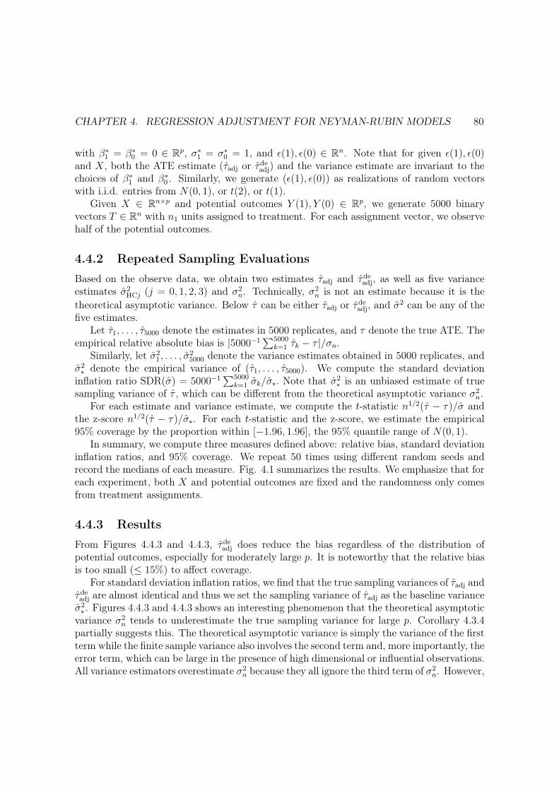
CHAPTER 4. REGRESSION ADJUSTMENT FOR NEYMAN-RUBIN MODELS 80
with �⇤1= �⇤
0= 0 2 Rp, �⇤
1= �⇤
0= 1, and ✏(1), ✏(0) 2 Rn. Note that for given ✏(1), ✏(0)
and X, both the ATE estimate (⌧adj or ⌧deadj
) and the variance estimate are invariant to thechoices of �⇤
1and �⇤
0. Similarly, we generate (✏(1), ✏(0)) as realizations of random vectors
with i.i.d. entries from N(0, 1), or t(2), or t(1).Given X 2 Rn⇥p and potential outcomes Y (1), Y (0) 2 Rp, we generate 5000 binary
vectors T 2 Rn with n1 units assigned to treatment. For each assignment vector, we observehalf of the potential outcomes.
4.4.2 Repeated Sampling EvaluationsBased on the observe data, we obtain two estimates ⌧adj and ⌧de
adj, as well as five variance
estimates �2
HCj(j = 0, 1, 2, 3) and �2
n. Technically, �2
nis not an estimate because it is the
theoretical asymptotic variance. Below ⌧ can be either ⌧adj or ⌧deadj
, and �2 can be any of thefive estimates.
Let ⌧1, . . . , ⌧5000 denote the estimates in 5000 replicates, and ⌧ denote the true ATE. Theempirical relative absolute bias is |5000�1
P5000
k=1⌧k � ⌧ |/�n.
Similarly, let �2
1, . . . , �2
5000denote the variance estimates obtained in 5000 replicates, and
�2
⇤ denote the empirical variance of (⌧1, . . . , ⌧5000). We compute the standard deviationinflation ratio SDR(�) = 5000�1
P5000
k=1�k/�⇤. Note that �2
⇤ is an unbiased estimate of truesampling variance of ⌧ , which can be different from the theoretical asymptotic variance �2
n.
For each estimate and variance estimate, we compute the t-statistic n1/2(⌧ � ⌧)/� andthe z-score n1/2(⌧ � ⌧)/�⇤. For each t-statistic and the z-score, we estimate the empirical95% coverage by the proportion within [�1.96, 1.96], the 95% quantile range of N(0, 1).
In summary, we compute three measures defined above: relative bias, standard deviationinflation ratios, and 95% coverage. We repeat 50 times using different random seeds andrecord the medians of each measure. Fig. 4.1 summarizes the results. We emphasize that foreach experiment, both X and potential outcomes are fixed and the randomness only comesfrom treatment assignments.
4.4.3 ResultsFrom Figures 4.4.3 and 4.4.3, ⌧de
adjdoes reduce the bias regardless of the distribution of
potential outcomes, especially for moderately large p. It is noteworthy that the relative biasis too small ( 15%) to affect coverage.
For standard deviation inflation ratios, we find that the true sampling variances of ⌧adj and⌧deadj
are almost identical and thus we set the sampling variance of ⌧adj as the baseline variance�2
⇤. Figures 4.4.3 and 4.4.3 shows an interesting phenomenon that the theoretical asymptoticvariance �2
ntends to underestimate the true sampling variance for large p. Corollary 4.3.4
partially suggests this. The theoretical asymptotic variance is simply the variance of the firstterm while the finite sample variance also involves the second term and, more importantly, theerror term, which can be large in the presence of high dimensional or influential observations.All variance estimators overestimate �2
nbecause they all ignore the third term of �2
n. However,

CHAPTER 4. REGRESSION ADJUSTMENT FOR NEYMAN-RUBIN MODELS 81
normal t(2) Cauchy
0.0 0.2 0.4 0.6 0.0 0.2 0.4 0.6 0.0 0.2 0.4 0.60.00
0.05
0.10
0.15
Exponent (log p / log n)
Rel
ative
Bia
s
tauhat_type un−debiased debiased
(a) Relative bias of ⌧deadj and ⌧adj.
normal t(2) Cauchy
0.0 0.2 0.4 0.6 0.0 0.2 0.4 0.6 0.0 0.2 0.4 0.60.50
0.75
1.00
1.25
1.50
Exponent (log p / log n)
Std.
Infla
ted
Rat
io
type HC0 HC1 HC2 HC3 theoretical
(b) Ratio of standard deviation between five standard de-
viation estimates, �n, �HC0, �HC1, �HC2, �HC3, and the true
standard deviation of ⌧adj.
normal t(2) Cauchy
un−debiaseddebiased
0.0 0.2 0.4 0.6 0.0 0.2 0.4 0.6 0.0 0.2 0.4 0.6
0.50
0.65
0.75
0.85
0.951.00
0.50
0.65
0.75
0.85
0.951.00
Exponent (log p / log n)
Cov
erag
e
type theoretical HC2 HC3
(c) Empirical 95% coverage of t-statistics derived from two
estimators and four variance estimators (“theoretical” for �2n,
“HC2” for �2HC2 and “HC3” for �2
HC3)
Figure 4.1: Simulation with ⇡1 = 0.2. X is a realization of a random matrix with i.i.d. t(2)entries, and e(t) is a realization of a random vector with i.i.d. entries from a distributioncorresponding to each column.

CHAPTER 4. REGRESSION ADJUSTMENT FOR NEYMAN-RUBIN MODELS 82
normal t(2) Cauchy
0.0 0.2 0.4 0.6 0.0 0.2 0.4 0.6 0.0 0.2 0.4 0.60.00
0.05
0.10
0.15
Exponent (log p / log n)
Rel
ative
Bia
s
tauhat_type un−debiased debiased
(a) Relative bias of ⌧deadj and ⌧adj.
normal t(2) Cauchy
0.0 0.2 0.4 0.6 0.0 0.2 0.4 0.6 0.0 0.2 0.4 0.60.50
0.75
1.00
1.25
1.50
Exponent (log p / log n)
Std.
Infla
ted
Rat
io
type HC0 HC1 HC2 HC3 theoretical
(b) Ratio of standard deviation between five standard de-
viation estimates, �n, �HC0, �HC1, �HC2, �HC3, and the true
standard deviation of ⌧adj.
normal t(2) Cauchy
un−debiaseddebiased
0.0 0.2 0.4 0.6 0.0 0.2 0.4 0.6 0.0 0.2 0.4 0.6
0.50
0.65
0.75
0.85
0.951.00
0.50
0.65
0.75
0.85
0.951.00
Exponent (log p / log n)
Cov
erag
e
type theoretical HC2 HC3
(c) empirical 95% coverage of t-statistics derived from two
estimators and four variance estimators (“theoretical” for �2n,
“HC2” for �2HC2 and “HC3” for �2
HC3)
Figure 4.2: Simulation. X is a realization of a random matrix with i.i.d. t(2) entries, ande(t) is a realization of a random vector with i.i.d. entries from a distribution correspondingto each column.

CHAPTER 4. REGRESSION ADJUSTMENT FOR NEYMAN-RUBIN MODELS 83
all estimators, except the HC3 estimator, tend to underestimate the true sampling variancefor large p. In contrast, the HC3 estimator does not suffer from anti-conservatism.
Figures 4.4.3 and 4.4.3 shows that HC0 and HC1 variance estimates lie between thetheoretical asymptotic variance and the HC2 variance estimate. For better visualization,we only plot the 95% coverage of t-statistics computed from �2
n, �2
HC2and �2
HC3in Figures
4.4.3 and 4.4.3. We draw the following conclusions from Figures 4.4.3 and 4.4.3. First, aswe pointed out previously, the coverage of two ATE estimates are almost identical becausethe relative bias is small in these scenarios. Second, as Figures 4.4.3 and 4.4.3 suggest, thet-statistic with HC3 variance estimate has the best coverage, and it protects the coverageagainst the increasing dimension. In contrast, the theoretical asymptotic variance and HCj(j = 0, 1, 2) variance estimates yield significantly lower coverage for large p. Therefore, weadvocate using �2
HC3for variance estimation.
4.4.4 Effectiveness of debiasingIn the aforementioned settings, the debiased estimator yields almost identical inference asthe undebiased estimator. This is not surprising because in the above scenarios the potentialoutcomes are generated from linear models and thus Lin (2013)’s estimator has bias close tozero. However, in practice, the potential outcomes might not have prefect linear relationshipswith the covariates. To illustrate the potential benefits of debiasing, we consider the “most-biased” situation which maximizes the “bias term”, measured as the second term in theexpansion (4.18). Specifically, we consider the case where ✏(0) = ✏ and ✏(1) = 2✏ for somevector ✏ that satisfies (4.7) with sample variance 1. To maximize the bias term, we take ✏ asthe solution of
max✏2Rn
����n1
n0
�0 �n0
n1
�1
���� =✓2n0
n1
� n1
n0
◆ ����nX
i=1
Hii✏i
����, (4.27)
s.t. k✏k22/n = 1, XT✏ = 1T✏ = 0.
We give more details of constructing ✏ in Section C.6 of Supplementary Material III. From(4.27), the bias is amplified when the group sizes are unbalanced. Note that this settingessentially assume a non-linear relationship between the potential outcomes and the covari-ates.
We perform simulation detailed in Section 4.4.2 based on potential outcomes in (4.27)and report relative bias and coverage to demonstrate the effectiveness of debiasing. To savespace, we only report the coverage for �2
HC2and �2
HC3. Fig. 4.3 summarizes the results.
Unlike the previous settings, the relative bias in this setting is large enough to affect thecoverage. From Fig. 4.4.4, as expected, we see that the relative bias is larger when the groupsizes are more unbalanced. The debiased estimator reduces a fair proportion of bias in bothcases and improves coverage especially when the dimension is high. We provide experimentalresults in more settings in Supplementary Material III, which confirm the effectiveness ofdebiasing.

CHAPTER 4. REGRESSION ADJUSTMENT FOR NEYMAN-RUBIN MODELS 84
0
2
4
6
0.0 0.2 0.4 0.6
Exponent (log p / log n)
Rel
ative
Bia
s
tauhat_type un−debiased debiased
0
2
4
6
0.0 0.2 0.4 0.6
Exponent (log p / log n)
Rel
ative
Bia
s
tauhat_type un−debiased debiased
(a) Relative bias of ⌧deadj and ⌧adj.
HC2 HC3
0.0 0.2 0.4 0.6 0.0 0.2 0.4 0.60.00
0.25
0.50
0.650.750.850.951.00
Exponent (log p / log n)
Cov
erag
e
tauhat_type un−debiased debiased
HC2 HC3
0.0 0.2 0.4 0.6 0.0 0.2 0.4 0.60.00
0.25
0.50
0.650.750.850.951.00
Exponent (log p / log n)
Cov
erag
e
tauhat_type un−debiased debiased
(b) Empirical 95% coverage of t-statistics derived from two estimators and two variance estimators
(“HC2” for �2HC2 and “HC3” for �2
HC3)
Figure 4.3: Simulation. X is a realization of a random matrix with i.i.d. t(2) entries ande(t) is defined in (4.27): (Left) ⇡1 = 0.2; (Right) ⇡1 = 0.5.
4.4.5 Trimming the Design MatrixOur theory suggests that of the design matrix affects the statistical properties of ⌧adj and⌧deadj
. When there are many influential observations in the data, it is beneficial to reduce before regression adjustment. Because our theory holds even for mis-specified linear models,any preprocessing of X does not affect the consistency and asymptotic normality if thepreprocessing does not depend on T or Y obs. This is a feature of our theory. In contrast,trimming is not applicable to the theory under a super-population perspective assuming acorrectly specified regression model.

CHAPTER 4. REGRESSION ADJUSTMENT FOR NEYMAN-RUBIN MODELS 85
HC2 HC3
0.0 0.2 0.4 0.6 0.0 0.2 0.4 0.60.00
0.20
0.50
0.650.750.850.951.00
Exponent (log p / log n)
Cov
erag
e
Regularization FALSE TRUE
HC2 HC3
0.0 0.2 0.4 0.6 0.0 0.2 0.4 0.60.00
0.20
0.50
0.650.750.850.951.00
Exponent (log p / log n)
Cov
erag
e
Regularization FALSE TRUE
Figure 4.4: Simulation. Empirical 95% coverage of t-statistics derived from the debiasedestimator with and without trimming the covariate matrix: (Left) ⇡1 = 0.2; (Right) ⇡1 = 0.5.X is a realization of a random matrix with i.i.d. t(2) entries and e(t) is defined in (4.27).
In Section 4.4, the entries of X are realizations of heavy-tailed random variables, and increases even with an infrequent extreme covariate value. For the 50 design matrices usedin Section 4.4 with p = dn2/3e and n = 2000, the average of is 0.9558 with standard error0.0384. Now we consider a simple form of trimming which thresholds each column at its 2.5%and 97.5% quantiles. Then the average of reduces dramatically to 0.0704 with standarderror 0.0212. Fig. 4.4 shows the coverage of the t-statistics derived from ⌧de
adjwith and
without the trimming. It is clear that the coverage gets drastically improved after trimming.Since the main goal of this chapter is not on statistical methodology, we only propose
the above heuristic approach to illustrate the idea of trimming, motivated by our asymptotictheory. The general methodology is an interesting future research topic.
4.5 Conclusions and Practical Suggestions
Fisher (1935b) advocated using the analysis of covariance under treatment-unit additivity.Freedman (2008b) highlighted its dangers under treatment effect heterogeneity. Lin (2013)proposed a simple OLS estimator with treatment-covariate interactions accounting for po-tential heterogeneity. We establish the consistency and the asymptotic normality of Lin(2013)’s estimator allowing for a growing dimension of the covariates. We further propose adebiased estimator which permits valid inference in broader asymptotic regimes.
In summary, we find that the classical inferential procedure tends to be invalid whenthe design matrix has many covariates or many influential observations. In these scenarios,the bias blows up and the variance estimation becomes anti-conservative. We suggest usingthe debiased estimator (4.10) and the HC3 variance estimator for inference. In addition, wesuggest trimming the design matrix to reduce the extreme leverage scores before regressionadjustment.

CHAPTER 4. REGRESSION ADJUSTMENT FOR NEYMAN-RUBIN MODELS 86
4.6 Technical Lemmas
4.6.1 Some general results for sampling without replacementCompletely randomized experiments have deep connections with sampling without replace-ment because the treatment and control groups are simple random samples from a finitepopulation of n units. Below we use T to denote a random size-m subset of {1, . . . , n} overall
�n
m
�subsets, and Sp�1 = {(!1, . . . ,!p)T : !2
1+ · · · + !2
p= 1} to denote the (p � 1)-
dimensional unit sphere.The first lemma gives the mean and variance of the sample total from sampling without
replacement. See Cochran (2007, Theorem 2.2) for a proof.
Lemma 4.6.1. Let (w1, . . . , wn) be fixed scalars with mean w = n�1P
n
i=1wi. Then
Pi2T wi
has mean mw and variance
Var
X
i2T
wi
!=
m(n�m)
n(n� 1)
nX
i=1
(wi � w)2.
The second lemma gives the Berry–Esseen-type bound for the finite population centrallimit theorem. See Bikelis (1969) and Höglund (1978) for proofs.
Lemma 4.6.2. Let (w1, . . . , wn) be fixed scalars with w = n�1P
n
i=1wi and S2
w=P
n
i=1(wi�
w)2. Let m = nf for some f 2 (0, 1). Then
dK
Pi2T (wi � w)
Sw
pf(1� f)
, N(0, 1)
! Cp
f(1� f)
Pn
i=1(wi � w)2
S3w
Cpf(1� f)
max1in |wi � w|Sw
,
where dK denotes the Kolmogorov distance between two distributions, and C is a universalconstant.
The following two lemmas give novel vector and matrix concentration inequalities forsampling without replacement.
Lemma 4.6.3. Let (u1, . . . , un) be a finite population of p-dimensional vectors withPn
i=1ui = 0. Then for any � 2 (0, 1), with probability 1� �
�����X
i2T
ui
�����2
kUkF
sm(n�m)
n(n� 1)+ kUkop
r8 log
1
�
where uTi
is the i-th row of the matrix U 2 Rn⇥p.

CHAPTER 4. REGRESSION ADJUSTMENT FOR NEYMAN-RUBIN MODELS 87
Lemma 4.6.4. Let (V1, . . . , Vn) be a finite population of (p ⇥ p)-dimensional Hermittianmatrices with
Pn
i=1Vi = 0. Let C(p) = 4(1 + d2 log pe), and
⌫2 =
�����1
n
nX
i=1
V 2
i
�����op
, ⌫2� = sup!2Sp�1
1
n
nX
i=1
(!TVi!)2, ⌫+ = max
1in
kVikop.
Then for any � 2 (0, 1), with probability 1� �,�����X
i2T
Vi
�����op
pnC(p)⌫ + C(p)⌫+ +
r8n log
1
�⌫�.
The following lemma gives the mean and variance of the summation over randomlyselected rows and columns from a deterministic matrix Q 2 Rn⇥n.
Lemma 4.6.5. Let Q 2 Rn⇥n be a deterministic matrix, and QT ⌘P
i,j2T Qij. Assumen � 4. Then
EQT =m(n�m)
n(n� 1)tr(Q) +
m(m� 1)
n(n� 1)1TQ1.
If Q further satisfies 1TQ = Q1 = 0, then
Var(QT ) m(n�m)
n(n� 1)kQk2
F.
Lemmas 4.6.3–4.6.5 are critical for our proofs. The proofs are relegated to SupplementaryMaterial I. They are novel tools to the best of our knowledge and potentially useful in othercontexts such as survey sampling, matrix sketching, and transductive learning.
4.6.2 Some results particularly useful for our settingWe first give an implication of Assumption 3, a lower bound on �2
nunder Assumption 1.
Lemma 4.6.6. Under Assumptions 1 and 3, �2
n� ⌘min {n1/n0, n0/n1} E2.
Recall Ht = Xt(XTtXt)�1XT
tand define ⌃t = n�1
t XTtXt (t = 0, 1). The following explicit
formula is the starting point of our proof.
Lemma 4.6.7. We have
⌧adj � ⌧ =1Te1(1)/n1 � 1TH1e1(1)/n1
1� 1TH11/n1
� 1Te0(0)/n0 � 1TH0e0(0)/n0
1� 1TH01/n0
. (4.28)
The quantities µt, e(t), and our estimators (⌧adj, ⌧deadj) are all invariant if X is transformed
to XZ for any full rank matrix Z 2 Rp⇥p, provided that (4.2) holds. Thus, without loss ofgenerality, we assume
n�1XTX = I. (4.29)

CHAPTER 4. REGRESSION ADJUSTMENT FOR NEYMAN-RUBIN MODELS 88
Otherwise, suppose X has the singular value decomposition U⌃V T with U 2 Rn⇥p,⌃, V 2Rp⇥p, then we can replace X by n1/2U = X(n1/2V ⌃�1) to ensure (4.29). We can verify thatthe key properties in (4.7) still hold. Assuming (4.29), we can rewrite the hat matrix andthe leverage scores as
H = n�1XXT, Hii = n�1kxik22, Hij = n�1xTixj. (4.30)
Note that the invariance property under the standardization (4.29) is a feature of the OLS-based regression adjustment. It does not hold for many other estimators (e.g., Bloniarz et al.2016; Wager et al. 2016).
We will repeatedly use the following results to obtain the stochastic orders of the termsin (4.28). They are consequences of Lemmas 4.6.3 and 4.6.4.
Lemma 4.6.8. Under Assumption 1, for t = 0, 1,
1Tet(t)
nt
= OP
rE2n
!,
����XT
t1
nt
����2
= OP
✓rp
n
◆,
����XT
tet(t)
nt
����2
= OP
⇣pE2
⌘.
Lemma 4.6.9. Under Assumptions 1, 2 and (4.29), for t = 0, 1,
k⌃t � Ikop
= OP
⇣p log p
⌘,
��⌃�1
t
��op
= OP(1),��⌃�1
t� I
��op
= OP
⇣p log p
⌘.
The following lemma states some key properties of an intermediate quantity, which willfacilitate our proofs.
Lemma 4.6.10. Define Q(t) = H diag (e(t)) = (Hijej(t))n
i,j=1. It satisfies
1TQ(t) = 0, Q(t)1 = 0, 1TQ(t)1 = 0,
tr(Q(t)) = n�t, kQ(t)k2F=
nX
i=1
e2i(t)Hii nE2.
4.7 Proofs of The Main Results
4.7.1 Proof of the asymptotic expansionsProof of Theorem 4.3.3. We need to analyze the terms in (4.28). First, by Lemmas 4.6.8and 4.6.9,
1THt1nt
=1TXt
nt
⌃�1
t
XTt1
nt
��⌃�1
t
��op
����XT
t1
nt
����2
2
= OP
⇣pn
⌘.

CHAPTER 4. REGRESSION ADJUSTMENT FOR NEYMAN-RUBIN MODELS 89
Using (4.17) that p = o(n), we obtain that
1
1� 1THt1/nt
= 1 +OP
⇣pn
⌘. (4.31)
Second,
1THtet(t)
nt
=1TXt
nt
⌃�1
t
XTtet(t)
nt
=1TXt
nt
XTtet(t)
nt
+1TXt
nt
�⌃�1
t� I
� XTtet(t)
nt
⌘ Rt1 +Rt2. (4.32)
Note that here we do not use the naive bound for 1THtet(t)/nt as for 1THt1/nt in (4.31)because this gives weaker results. Instead, we bound Rt1 and Rt2 separately. Lemmas 4.6.8and 4.6.9 imply
Rt2 ��⌃�1
t� I
��op
����XT
t1
nt
����2
����XT
tet(t)
nt
����2
= OP
rE22p log p
n
!. (4.33)
We apply Chebyshev’s inequality to obtain that
Rt1 = ERt1 +OP
⇣pVar(Rt1)
⌘. (4.34)
Therefore, to bound Rt1, we need to calculate its first two moments. Recalling (4.30) andthe definition of Q(t) in Lemma 4.6.10, we have
Rt1 =1
n2
t
X
i2Tt
xTi
! X
i2Tt
xiei(t)
!=
1
n2
t
X
i2Tt
X
j2Tt
xTixjej(t)
=1
n2
t
X
i2Tt
X
j2Tt
nHijej(t) =n
n2
t
X
i2Tt
X
j2Tt
Qij(t). (4.35)
Lemmas 4.6.5 and 4.6.10 imply the expectation of Rt1:
ERt1 =n
n2
t
✓n1n0
n(n� 1)tr (Q(t)) +
nt(nt � 1)
n(n� 1)1TQ(t)1
◆
=nn1n0
n2
t (n� 1)�t =
n1n0
n2
t
�t +O
✓|�t|n
◆. (4.36)
We then bound the variance of Rt1:
Var(Rt1) =n2
n4
t
Var
X
i,j2Tt
Qij(t)
! n2
n4
t
n1n0
n(n� 1)kQ(t)k2
F(4.37)

CHAPTER 4. REGRESSION ADJUSTMENT FOR NEYMAN-RUBIN MODELS 90
n2
n4
t
n1n0
n(n� 1)nE2 = O
✓E2n
◆, (4.38)
where (4.37) follows from Lemma 4.6.5, (4.38) follows from Lemma 4.6.10 and Assumption1. Putting (4.32)–(4.36) and (4.38) together, we obtain that
1THtet(t)
nt
=n1n0
n2
t
�t +OP
rE22p log p
n+
|�t|n
+
rE2n
!(4.39)
By (4.20) and (4.17) that p = o(n), (4.39) further simplifies to
1THtet(t)
nt
=n1n0
n2
t
�t +OP
rE22p log p
n+
rE2n
!. (4.40)
Using Lemma 4.6.8, (4.40), and the fact that 1, we have
1Tet(t)nt
� 1THtet(t)
nt
= OP
rE2n
+�+
rE22p log p
n
!. (4.41)
Finally, putting (4.31), (4.40) and (4.41) together into (4.28), we obtain that
⌧adj � ⌧ =
✓1Te1(1)
n1
� 1TH1e1(1)
n1
◆⇣1 +OP
⇣pn
⌘⌘
�✓
1Te0(0)n0
� 1TH0e0(0)
n0
◆⇣1 +OP
⇣pn
⌘⌘
=1Te1(1)
n1
� 1Te0(0)n0
+1TH0e0(0)
n0
� 1TH1e1(1)
n1
+OP
rp2E2n3
+p�
n+
rE22p3 log p
n3
!
=1Te1(1)
n1
� 1Te0(0)n0
+n1
n0
�0 �n0
n1
�1
+OP
rp2E2n3
+p�
n+
rE22p log p
n+
rE2n
!. (4.42)
where (4.42) uses (4.17) that p = o(n). The fourth terms dominates the first term in (4.42)because p = o(n) and � p/n. The third term dominates the second term in (4.42) because,by (4.20),
p�
n �
p� = O
rE22pn
!.
Deleting the first two terms in (4.42), we complete the proof.

CHAPTER 4. REGRESSION ADJUSTMENT FOR NEYMAN-RUBIN MODELS 91
Proof of Corollary 4.3.4. Assumption 1 implies n1n0�0 � n0
n1�1 = O (�) , which, coupled with
Theorem 4.3.3, implies (4.21).The key is to prove the result for the debiased estimator. By definition,
⌧deadj
� ⌧ =1Te1(1)
n1
� 1Te0(0)n0
+n1
n0
(�0 � �0)�n0
n1
(�1 � �1)
+OP
rE22p log p
n+
rE2n
!,
and therefore, the key is to bound |�t � �t|.We introduce an intermediate quantity �t = n�1
t
Pi2Tt Hiiei(t). It has mean E�t = �t
and variance
Var(�t) 1
n2
t
n1n0
n(n� 1)
nX
i=1
H2
iie2i(t) E22
n2
t
= O
✓E22
n
◆, (4.43)
from Lemma 4.6.1 and Assumption 1. Equipped with the first two moments, we use Cheby-shev’s inequality to obtain
|�t ��t| = OP
rE22n
!. (4.44)
Next we bound |�t � �t|. The Cauchy–Schwarz inequality implies
|�t � �t| 1
nt
X
i2Tt
Hii|ei � ei(t)| s
1
nt
X
i2Tt
H2
ii
s1
nt
X
i2Tt
(ei � ei(t))2. (4.45)
First,1
nt
X
i2Tt
H2
ii n
nt
1
n
nX
i=1
Hii
!= O
⇣pn
⌘. (4.46)
Second, using the fact et = (I �Ht)et(t), we have
1
nt
X
i2Tt
(ei � ei(t))2 =
1
nt
ket � et(t)k22 =1
nt
eTt(t)Htet(t)
=
✓XT
tet(t)
nt
◆T
⌃�1
t
XTtet(t)
nt
k⌃tk�1
op
����XT
tet(t)
nt
����2
2
= OP(E2), (4.47)
where the last line follows from Lemma 4.6.8. Putting (4.46) and (4.47) into (4.45), weobtain
|�t � �t| = OP
rE22pn
!. (4.48)
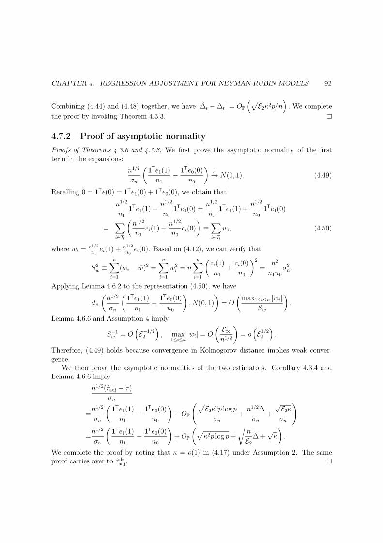
CHAPTER 4. REGRESSION ADJUSTMENT FOR NEYMAN-RUBIN MODELS 92
Combining (4.44) and (4.48) together, we have |�t ��t| = OP
⇣pE22p/n
⌘. We complete
the proof by invoking Theorem 4.3.3.
4.7.2 Proof of asymptotic normalityProofs of Theorems 4.3.6 and 4.3.8. We first prove the asymptotic normality of the firstterm in the expansions:
n1/2
�n
✓1Te1(1)
n1
� 1Te0(0)n0
◆d! N(0, 1). (4.49)
Recalling 0 = 1Te(0) = 1Te1(0) + 1Te0(0), we obtain that
n1/2
n1
1Te1(1)�n1/2
n0
1Te0(0) =n1/2
n1
1Te1(1) +n1/2
n0
1Te1(0)
=X
i2Tt
✓n1/2
n1
ei(1) +n1/2
n0
ei(0)
◆⌘X
i2Tt
wi, (4.50)
where wi =n1/2
n1ei(1) +
n1/2
n0ei(0). Based on (4.12), we can verify that
S2
w⌘
nX
i=1
(wi � w)2 =nX
i=1
w2
i= n
nX
i=1
✓ei(1)
n1
+ei(0)
n0
◆2
=n2
n1n0
�2
n.
Applying Lemma 4.6.2 to the representation (4.50), we have
dK
✓n1/2
�n
✓1Te1(1)
n1
� 1Te0(0)n0
◆, N(0, 1)
◆= O
✓max1in |wi|
Sw
◆.
Lemma 4.6.6 and Assumption 4 imply
S�1
w= O
⇣E�1/2
2
⌘, max
1in
|wi| = O
✓E1n1/2
◆= o
⇣E1/2
2
⌘.
Therefore, (4.49) holds because convergence in Kolmogorov distance implies weak conver-gence.
We then prove the asymptotic normalities of the two estimators. Corollary 4.3.4 andLemma 4.6.6 imply
n1/2(⌧adj � ⌧)
�n
=n1/2
�n
✓1Te1(1)
n1
� 1Te0(0)n0
◆+OP
pE22p log p�n
+n1/2�
�n+
pE2�n
!
=n1/2
�n
✓1Te1(1)
n1
� 1Te0(0)n0
◆+OP
✓p2p log p+
rn
E2�+
p
◆.
We complete the proof by noting that = o(1) in (4.17) under Assumption 2. The sameproof carries over to ⌧de
adj.
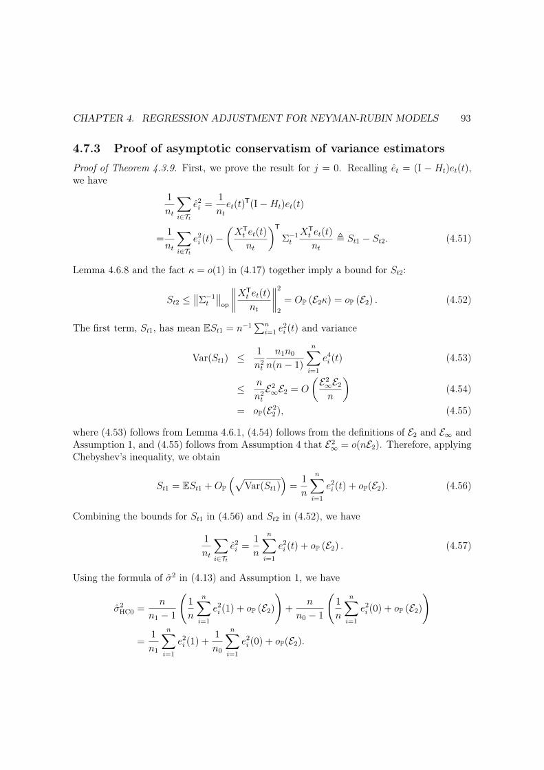
CHAPTER 4. REGRESSION ADJUSTMENT FOR NEYMAN-RUBIN MODELS 93
4.7.3 Proof of asymptotic conservatism of variance estimatorsProof of Theorem 4.3.9. First, we prove the result for j = 0. Recalling et = (I � Ht)et(t),we have
1
nt
X
i2Tt
e2i=
1
nt
et(t)T(I �Ht)et(t)
=1
nt
X
i2Tt
e2i(t)�
✓XT
tet(t)
nt
◆T
⌃�1
t
XTtet(t)
nt
, St1 � St2. (4.51)
Lemma 4.6.8 and the fact = o(1) in (4.17) together imply a bound for St2:
St2 ��⌃�1
t
��op
����XT
tet(t)
nt
����2
2
= OP (E2) = oP (E2) . (4.52)
The first term, St1, has mean ESt1 = n�1P
n
i=1e2i(t) and variance
Var(St1) 1
n2
t
n1n0
n(n� 1)
nX
i=1
e4i(t) (4.53)
n
n2
t
E2
1E2 = O
✓E2
1E2n
◆(4.54)
= oP(E2
2), (4.55)
where (4.53) follows from Lemma 4.6.1, (4.54) follows from the definitions of E2 and E1 andAssumption 1, and (4.55) follows from Assumption 4 that E2
1 = o(nE2). Therefore, applyingChebyshev’s inequality, we obtain
St1 = ESt1 +OP
⇣pVar(St1)
⌘=
1
n
nX
i=1
e2i(t) + oP(E2). (4.56)
Combining the bounds for St1 in (4.56) and St2 in (4.52), we have
1
nt
X
i2Tt
e2i=
1
n
nX
i=1
e2i(t) + oP (E2) . (4.57)
Using the formula of �2 in (4.13) and Assumption 1, we have
�2
HC0=
n
n1 � 1
1
n
nX
i=1
e2i(1) + oP (E2)
!+
n
n0 � 1
1
n
nX
i=1
e2i(0) + oP (E2)
!
=1
n1
nX
i=1
e2i(1) +
1
n0
nX
i=1
e2i(0) + oP(E2).

CHAPTER 4. REGRESSION ADJUSTMENT FOR NEYMAN-RUBIN MODELS 94
Using the formula of �2
nin (4.11), we have
�2
HC0� �2
n+
1
n
nX
i=1
(ei(1)� ei(0))2 + oP(E2) � �2
n+ oP(E2),
which, coupled with Lemma 4.6.6, implies that �2
HC0/�2
n� 1 + oP(1).
Next we prove that the �2
HCj’s are asymptotically equivalent. It suffices to show that
minj=1,2,3
min1in
|ei,j|/|ei| = 1 + oP(1). (4.58)
The proof for j = 1 follows from p/n = o(1) in (4.17). To prove (4.58) for j = 2, 3, we needto prove that maxt=0,1 maxi2Tt Ht,ii = oP(1). This follows from Lemma 4.6.9 and the fact that = o(1) in (4.17):
maxi2Tt
Ht,ii = maxi2Tt
n�1
txTi⌃�1
txi = OP
✓n�1
tmax1in
kxik22◆
= OP () .

95
Bibliography
Abadie, A., S. Athey, G. W. Imbens, and J. M. Wooldridge (2017). “Sampling-based vs.design-based uncertainty in regression analysis”. In: arXiv preprint arXiv:1706.01778.
Adichie, J. N. (1967a). “Asymptotic efficiency of a class of non-parametric tests for regressionparameters”. In: The Annals of Mathematical Statistics, pp. 884–893.
— (1978). “Rank tests of sub-hypotheses in the general linear regression”. In: The Annals ofStatistics 6.5, pp. 1012–1026.
— (1984). “11 Rank tests in linear models”. In: Handbook of statistics 4, pp. 229–257.Adichie, J. N. (1967b). “Estimates of regression parameters based on rank tests”. In: The
Annals of Mathematical Statistics, pp. 894–904.Akritas, M. G. (1990). “The rank transform method in some two-factor designs”. In: Journal
of the American Statistical Association 85.409, pp. 73–78.Akritas, M. G. and S. Arnold (2000). “Asymptotics for analysis of variance when the number
of levels is large”. In: Journal of the American Statistical association 95.449, pp. 212–226.Akritas, M. G. and S. F. Arnold (1994). “Fully nonparametric hypotheses for factorial de-
signs I: Multivariate repeated measures designs”. In: Journal of the American StatisticalAssociation 89.425, pp. 336–343.
Akritas, M. G., S. F. Arnold, and E. Brunner (1997). “Nonparametric hypotheses and rankstatistics for unbalanced factorial designs”. In: Journal of the American Statistical Asso-ciation 92.437, pp. 258–265.
Alimoradi, S. and A. M. E. Saleh (1998). “9 On some L-estimation in linear regressionmodels”. In: Handbook of Statistics 17, pp. 237–280.
Anatolyev, S. (2012). “Inference in regression models with many regressors”. In: Journal ofEconometrics 170.2, pp. 368–382.
Anatolyev, S. and P. Yaskov (2017). “Asymptotics of diagonal elements of projection matricesunder many instruments/regressors”. In: Econometric Theory 33, pp. 717–738.
Anderson, M. J. and J. Robinson (2001). “Permutation tests for linear models”. In: Australian& New Zealand Journal of Statistics 43.1, pp. 75–88.
Anderson, T. W. (1962). An introduction to multivariate statistical analysis. Wiley NewYork.
Angrist, J., D. Lang, and P. Oreopoulos (2009). “Incentives and services for college achieve-ment: Evidence from a randomized trial”. In: American Economic Journal: Applied Eco-nomics 1, pp. 136–63.
BIBLIOGRAPHY 96
Arnold, S. F. (1980). “Asymptotic validity of F tests for the ordinary linear model and themultiple correlation model”. In: Journal of the American Statistical Association 75.372,pp. 890–894.
Aubuchon, J. C. and T. P. Hettmansperger (1984). “12 On the use of rank tests and estimatesin the linear model”. In: Handbook of statistics 4, pp. 259–274.
Bahr, B. von and C.-G. Esseen (1965). “Inequalities for the r th Absolute Moment of aSum of Random Variables, 1 r 2”. In: The Annals of Mathematical Statistics 36,pp. 299–303.
Bai, Z. and Y. Wu (1994). “Limiting behavior of M-estimators of regression coefficientsin high dimensional linear models I. scale dependent case”. In: Journal of MultivariateAnalysis 51.2, pp. 211–239.
Bai, Z. and Y. Yin (1993). “Limit of the smallest eigenvalue of a large dimensional samplecovariance matrix”. In: The annals of Probability, pp. 1275–1294.
Bai, Z. and J. W. Silverstein (2010). Spectral analysis of large dimensional random matrices.Vol. 20. Springer.
Baranchik, A. (1973). “Inadmissibility of maximum likelihood estimators in some multiple re-gression problems with three or more independent variables”. In: The Annals of Statistics,pp. 312–321.
Barber, R. F., E. J. Candès, et al. (2015). “Controlling the false discovery rate via knockoffs”.In: The Annals of Statistics 43.5, pp. 2055–2085.
Bardenet, R. and O.-A. Maillard (2015). “Concentration inequalities for sampling withoutreplacement”. In: Bernoulli 21.3, pp. 1361–1385.
Bartlett, M. (1935). “The effect of non-normality on the t distribution”. In: mathematicalproceedings of the cambridge philosophical society. Vol. 31. Cambridge University Press,pp. 223–231.
Bathke, A. C. and S. W. Harrar (2008). “Nonparametric methods in multivariate factorialdesigns for large number of factor levels”. In: Journal of Statistical planning and Inference138.3, pp. 588–610.
Bathke, A. and D. Lankowski (2005). “Rank procedures for a large number of treatments”.In: Journal of statistical planning and inference 133.2, pp. 223–238.
Bean, D., P. J. Bickel, N. El Karoui, C. Lim, and B. Yu (2012). “Penalized robust regressionin high-dimension”. In: Technical Report 813, Department of Statistics, UC Berkeley.
Bean, D., P. J. Bickel, N. El Karoui, and B. Yu (2013). “Optimal M-estimation in high-dimensional regression”. In: Proceedings of the National Academy of Sciences 110.36,pp. 14563–14568.
Benjamini, Y. (1983). “Is the t test really conservative when the parent distribution is long-tailed?” In: Journal of the American Statistical Association 78.383, pp. 645–654.
Berk, R., E. Pitkin, L. Brown, A. Buja, E. George, and L. Zhao (2013). “Covariance adjust-ments for the analysis of randomized field experiments”. In: Evaluation review 37.3-4,pp. 170–196.
Berry, K. J., J. E. Johnston, and P. W. Mielke (2013). A chronicle of permutation statisticalmethods. 1920-2000, and beyond. Springer. doi: 10.1007/978-3-319-02744-9.

BIBLIOGRAPHY 97
Bhattacharya, R. N. and J. K. Ghosh (1978). “On the validity of the formal Edgeworthexpansion”. In: Ann. Statist 6.2, pp. 434–451.
Bickel, P. J. and E. L. Lehmann (1975). “Descriptive Statistics for Nonparametric ModelsII. Location”. In: The Annals of Statistics 3.5, pp. 1045–1069.
Bickel, P. J. (1965). “On some robust estimates of location”. In: The Annals of MathematicalStatistics 36.3, pp. 847–858.
— (1973). “On some analogues to linear combinations of order statistics in the linear model”.In: The Annals of Statistics, pp. 597–616.
— (1975). “One-step Huber estimates in the linear model”. In: Journal of the AmericanStatistical Association 70.350, pp. 428–434.
Bickel, P. J. and K. A. Doksum (2015). Mathematical Statistics: Basic Ideas and SelectedTopics, volume I. Vol. 117. CRC Press.
Bickel, P. J. and D. A. Freedman (1981). “Some asymptotic theory for the bootstrap”. In:The Annals of Statistics, pp. 1196–1217.
— (1983a). “Bootstrapping regression models with many parameters”. In: Festschrift forErich L. Lehmann, pp. 28–48.
— (1983b). “Bootstrapping regression models with many parameters”. In: Festschrift forErich L. Lehmann, pp. 28–48.
Bickel, P. J. and A. Sakov (2008). “On the choice of m in the m out of n bootstrap andconfidence bounds for extrema”. In: Statistica Sinica 18.3, pp. 967–985.
Bikelis, A. (1969). “On the estimation of the remainder term in the central limit theorem forsamples from finite populations”. In: Studia Sci. Math. Hungar 4, pp. 345–354.
Bloniarz, A., H. Liu, C.-H. Zhang, J. S. Sekhon, and B. Yu (2016). “Lasso adjustments oftreatment effect estimates in randomized experiments”. In: Proceedings of the NationalAcademy of Sciences 113, pp. 7383–7390.
Bobkov, S. G. (2004). “Concentration of normalized sums and a central limit theorem fornoncorrelated random variables”. In: Annals of probability 32, pp. 2884–2907.
Boos, D. D. (1992). “On generalized score tests”. In: The American Statistician 46.4, pp. 327–333.
Boos, D. D. and C. Brownie (1995). “ANOVA and rank tests when the number of treatmentsis large”. In: Statistics & Probability Letters 23.2, pp. 183–191.
Boucheron, S., G. Lugosi, and P. Massart (2013). Concentration inequalities: A nonasymp-totic theory of independence. Oxford university press.
Box, G. E. (1953). “Non-normality and tests on variances”. In: Biometrika 40.3/4, pp. 318–335.
Box, G. E. and S. L. Andersen (1955). “Permutation theory in the derivation of robust criteriaand the study of departures from assumption”. In: Journal of the Royal Statistical Society:Series B (Methodological) 17.1, pp. 1–26.
Box, G. E. and G. S. Watson (1962). “Robustness to non-normality of regression tests”. In:Biometrika 49.1-2, pp. 93–106.
Brown, B. and J. Maritz (1982). “Distribution-Free Methods in Regression”. In: AustralianJournal of Statistics 24.3, pp. 318–331.

BIBLIOGRAPHY 98
Brown, G. W. and A. M. Mood (1951). “On median tests for linear hypotheses”. In: Proceed-ings of the Second Berkeley Symposium on Mathematical Statistics and Probability. TheRegents of the University of California.
Brownie, C. and D. D. Boos (1994). “Type I error robustness of ANOVA and ANOVA onranks when the number of treatments is large”. In: Biometrics, pp. 542–549.
Brunner, E. and M. Denker (1994). “Rank statistics under dependent observations and ap-plications to factorial designs”. In: Journal of Statistical planning and Inference 42.3,pp. 353–378.
Cai, T. T. and Z. Guo (2017). “Confidence intervals for high-dimensional linear regression:Minimax rates and adaptivity”. In: The Annals of statistics 45, pp. 615–646.
Calhoun, G. (2011). “Hypothesis testing in linear regression when k/n is large”. In: Journalof econometrics 165.2, pp. 163–174.
Campi, M. C., S. Ko, and E. Weyer (2009). “Non-asymptotic confidence regions for modelparameters in the presence of unmodelled dynamics”. In: Automatica 45.10, pp. 2175–2186.
Campi, M. C. and E. Weyer (2005). “Guaranteed non-asymptotic confidence regions in sys-tem identification”. In: Automatica 41.10, pp. 1751–1764.
Cattaneo, M. D., M. Jansson, and W. K. Newey (2018). “Inference in linear regression modelswith many covariates and heteroscedasticity”. In: Journal of the American StatisticalAssociation 113.523, pp. 1350–1361.
Chatterjee, S. B. (1999). “Generalised bootstrap techniques”. PhD thesis. Indian StatisticalInstitute, Kolkata.
Chatterjee, S. (2009). “Fluctuations of eigenvalues and second order Poincaré inequalities”.In: Probability Theory and Related Fields 143.1-2, pp. 1–40.
Chernoff, H. (1956). “Large-sample theory: Parametric case”. In: The Annals of MathematicalStatistics 27.1, pp. 1–22.
— (1981). “A note on an inequality involving the normal distribution”. In: The Annals ofProbability, pp. 533–535.
Chernozhukov, V., C. Hansen, and M. Jansson (2009). “Finite sample inference for quantileregression models”. In: Journal of Econometrics 152.2, pp. 93–103.
Chung, E. and J. P. Romano (2013). “Exact and asymptotically robust permutation tests”.In: The Annals of Statistics 41.2, pp. 484–507.
Cizek, P., W. K. Härdle, and R. Weron (2005). Statistical tools for finance and insurance.Springer Science & Business Media.
Cochran, W. G. (1937). “The Efficiencies of the Binomial Series Tests of Significance of aMean and of a Correlation Coefficient.” In: Journal of the Royal Statistical Society 100.1,pp. 69–73.
— (1977). Sampling Techniques. John Wiley & Sons.— (2007). Sampling Techniques. 3rd. New York: John Wiley & Sons.Collins, M. F. (1987). “A permutation test for planar regression”. In: Australian Journal of
Statistics 29.3, pp. 303–308.

BIBLIOGRAPHY 99
Conover, W. J. and R. L. Iman (1981). “Rank transformations as a bridge between parametricand nonparametric statistics”. In: The American Statistician 35.3, pp. 124–129.
Conover, W. and R. L. Iman (1976). “On some alternative procedures using ranks for theanalysis of experimental designs”. In: Communications in Statistics-Theory and Methods5.14, pp. 1349–1368.
Cornfield, J. (1944). “On samples from finite populations”. In: Journal of the AmericanStatistical Association 39.226, pp. 236–239.
Cortes, C., M. Mohri, D. Pechyony, and A. Rastogi (2009). “Stability analysis and learningbounds for transductive regression algorithms”. In: arXiv preprint arXiv:0904.0814.
Cressie, N. (1980). “Relaxing assumptions in the one sample t-test”. In: Australian Journalof Statistics 22.2, pp. 143–153.
Daniels, H. (1954). “A distribution-free test for regression parameters”. In: The Annals ofMathematical Statistics, pp. 499–513.
Das, D. and S. N. Lahiri (2019). “Second order correctness of perturbation bootstrap M-estimator of multiple linear regression parameter”. In: Bernoulli 25.1, pp. 654–682.
David, F. N. and N. Johnson (1951a). “The effect of non-normality on the power function ofthe F-test in the analysis of variance”. In: Biometrika 38.1/2, pp. 43–57.
David, F. and N. Johnson (1951b). “A method of investigating the effect of nonnormalityand heterogeneity of variance on tests of the general linear hypothesis”. In: The Annalsof Mathematical Statistics, pp. 382–392.
David, H. A. and H. N. Nagaraja (1981). Order statistics. Wiley Online Library.Dehejia, R. H. and S. Wahba (1999). “Causal effects in nonexperimental studies: Reevaluating
the evaluation of training programs”. In: Journal of the American Statistical Association94, pp. 1053–1062.
Diaconis, P. and M. Shahshahani (1987). “Time to reach stationarity in the Bernoulli–Laplacediffusion model”. In: SIAM Journal on Mathematical Analysis 18, pp. 208–218.
DiCiccio, C. J. and J. P. Romano (2017). “Robust permutation tests for correlation andregression coefficients”. In: Journal of the American Statistical Association 112.519,pp. 1211–1220.
Donoho, D. L. and X. Huo (2001). “Uncertainty principles and ideal atomic decomposition”.In: IEEE transactions on information theory 47, pp. 2845–2862.
Donoho, D. and A. Montanari (2016). “High dimensional robust m-estimation: Asymptoticvariance via approximate message passing”. In: Probability Theory and Related Fields166, pp. 935–969.
Donoho, D. and A. Montanari (2015). “Variance breakdown of Huber (M)-estimators: n/p !m 2 (1,1). arXiv preprint”. In: arXiv preprint arXiv:1503.02106.
Doob, J. L. (1935). “The limiting distributions of certain statistics”. In: The Annals of Math-ematical Statistics 6.3, pp. 160–169.
Draper, D. (1988). “Rank-based robust analysis of linear models. I. Exposition and review”.In: Statistical Science, pp. 239–257.
Durrett, R. (2010). Probability: theory and examples. Cambridge university press.

BIBLIOGRAPHY 100
Eden, T. and F. Yates (1933). “On the validity of Fisher’s z test when applied to an actualexample of non-normal data”. In: The Journal of Agricultural Science 23.1, pp. 6–17.
Eeden, C. van (1972). “An analogue, for signed rank statistics, of Jureckova’s asymptoticlinearity theorem for rank statistics”. In: The Annals of Mathematical Statistics 43.3,pp. 791–802.
Efron, B. (1979). “Bootstrap Methods: Another Look at the Jackknife”. In: The Annals ofStatistics 7.1, pp. 1–26.
Efron, B. (1969). “Student’s t-test under symmetry conditions”. In: Journal of the AmericanStatistical Association 64.328, pp. 1278–1302.
Efron, B. and B. Efron (1982). The jackknife, the bootstrap and other resampling plans.Vol. 38. SIAM.
Eicker, F. (1963). “Asymptotic normality and consistency of the least squares estimators forfamilies of linear regressions”. In: The Annals of Mathematical Statistics 34.2, pp. 447–456.
— (1967). “Limit theorems for regressions with unequal and dependent errors”. In: Proceed-ings of the fifth Berkeley symposium on mathematical statistics and probability. Vol. 1,pp. 59–82.
El Karoui, N. (2009). “Concentration of measure and spectra of random matrices: appli-cations to correlation matrices, elliptical distributions and beyond”. In: The Annals ofApplied Probability 19.6, pp. 2362–2405.
— (2010). “High-dimensionality effects in the Markowitz problem and other quadratic pro-grams with linear constraints: Risk underestimation”. In: The Annals of Statistics 38.6,pp. 3487–3566.
— (2013). “Asymptotic behavior of unregularized and ridge-regularized high-dimensionalrobust regression estimators: rigorous results”. In: arXiv preprint arXiv:1311.2445.
— (2015). “On the impact of predictor geometry on the performance on high-dimensionalridge-regularized generalized robust regression estimators”. In: Technical Report 826, De-partment of Statistics, UC Berkeley.
— (2018). “On the impact of predictor geometry on the performance on high-dimensionalridge-regularized generalized robust regression estimators”. In: Probability Theory andRelated Fields 170.1-2, pp. 95–175.
El Karoui, N., D. Bean, P. J. Bickel, C. Lim, and B. Yu (2013). “On robust regression withhigh-dimensional predictors”. In: Proceedings of the National Academy of Sciences 110.36,pp. 14557–14562.
El Karoui, N., D. Bean, P. J. Bickel, C. Lim, and B. Yu (2011). “On robust regressionwith high-dimensional predictors”. In: Technical Report 811, Department of Statistics,UC Berkeley.
El Karoui, N. and E. Purdom (2015). “Can we trust the bootstrap in high-dimension?” In:Technical Report 824, Department of Statistics, UC Berkeley.
— (2018). “Can we trust the bootstrap in high-dimensions? the case of linear models”. In:The Journal of Machine Learning Research 19.1, pp. 170–235.
BIBLIOGRAPHY 101
Esseen, C.-G. (1945a). “Fourier analysis of distribution functions. A mathematical study ofthe Laplace-Gaussian law”. In: Acta Mathematica 77.1, pp. 1–125.
— (1945b). “Fourier analysis of distribution functions. A mathematical study of the Laplace-Gaussian law”. In: Acta Mathematica 77.1, pp. 1–125.
Evans, R. D. and R. Evans (1955). Appendix G: The atomic nucleus. McGraw-Hill New York.Feng, L., C. Zou, Z. Wang, and B. Chen (2013). “Rank-based score tests for high-dimensional
regression coefficients”. In: Electronic Journal of Statistics 7, pp. 2131–2149.Feng, X., X. He, and J. Hu (2011). “Wild bootstrap for quantile regression”. In: Biometrika
98.4, pp. 995–999.Fisher, R. A. (1915). “Frequency distribution of the values of the correlation coefficient in
samples from an indefinitely large population”. In: Biometrika 10.4, pp. 507–521.— (1922). “The goodness of fit of regression formulae, and the distribution of regression
coefficients”. In: Journal of the Royal Statistical Society 85.4, pp. 597–612.— (1926). “The arrangement of field experiments”. In: Journal of the Ministry of Agriculture
33, pp. 503–513.— (1935a). “The logic of inductive inference”. In: Journal of the royal statistical society 98.1,
pp. 39–82.Fisher, R. A. (1924). “036: On a Distribution Yielding the Error Functions of Several
Well Known Statistics.” In: Proceedings of the International Congress of Mathematics2, pp. 805–813.
— (1925). Statistical methods for research workers. Oliver, Boyd, Edinburgh, and London.— (1935b). The Design of Experiments. 1st. Edinburgh: Oliver and Boyd.Fogarty, C. B. (2018). “Regression assisted inference for the average treatment effect in paired
experiments”. In: Biometrika, in press.Fogel, F., R. Jenatton, F. Bach, and A. d’Aspremont (2013). “Convex relaxations for per-
mutation problems”. In: Advances in Neural Information Processing Systems, pp. 1016–1024.
Freedman, D. A. (1981). “Bootstrapping regression models”. In: The Annals of Statistics 9.6,pp. 1218–1228.
— (2008a). “On regression adjustments in experiments with several treatments”. In: Theannals of applied statistics, pp. 176–196.
— (2008b). “On regression adjustments to experimental data”. In: Advances in AppliedMathematics 40, pp. 180–193.
Freedman, D. A. and D. Lane (1983). “A nonstochastic interpretation of reported significancelevels”. In: Journal of Business & Economic Statistics 1.4, pp. 292–298.
Friedman, M. (1937). “The use of ranks to avoid the assumption of normality implicit in theanalysis of variance”. In: Journal of the american statistical association 32.200, pp. 675–701.
— (1940). “A comparison of alternative tests of significance for the problem of m rankings”.In: The Annals of Mathematical Statistics 11.1, pp. 86–92.
Galton, F. (1894). Natural inheritance. Macmillan and Company.

BIBLIOGRAPHY 102
Gastwirth, J. L. (1966). “On robust procedures”. In: Journal of the American StatisticalAssociation 61.316, pp. 929–948.
Gayen, A. K. (1949). “The distribution of Student’s t in random samples of any size drawnfrom non-normal universes”. In: Biometrika 36.3/4, pp. 353–369.
— (1950). “The distribution of the variance ratio in random samples of any size drawn fromnon-normal universes”. In: Biometrika 37.3/4, pp. 236–255.
Geary, R. (1927). “Some properties of correlation and regression in a limited universe”. In:Metron 7, pp. 83–119.
Geary, R. C. (1947). “Testing for normality”. In: Biometrika 34.3/4, pp. 209–242.Geman, S. (1980). “A limit theorem for the norm of random matrices”. In: The Annals of
Probability, pp. 252–261.Gutenbrunner, C. and J. Jurecková (1992). “Regression quantile and regression rank score
process in the linear model and derived statistics”. In: Annals of Statistics 20, pp. 305–330.
Gutenbrunner, C., J. Jurečková, R. Koenker, and S. Portnoy (1993). “Tests of linear hy-potheses based on regression rank scores”. In: Journaltitle of Nonparametric Statistics2.4, pp. 307–331.
Hájek, J. (1960). “Limiting distributions in simple random sampling from a finite population”.In: Publications of the Mathematics Institute of the Hungarian Academy of Science 5,pp. 361–74.
Hájek, J. (1962). “Asymptotically most powerful rank-order tests”. In: The Annals of Math-ematical Statistics, pp. 1124–1147.
Hájek, J. and Z. Šidák (1967). Theory of rank tests. Academia.Hall, P. (1989). “Unusual properties of bootstrap confidence intervals in regression problems”.
In: Probability Theory and Related Fields 81.2, pp. 247–273.— (1992). The bootstrap and Edgeworth expansion. Springer Science & Business Media.Hanson, D. L. and F. T. Wright (1971). “A bound on tail probabilities for quadratic forms in
independent random variables”. In: The Annals of Mathematical Statistics 42.3, pp. 1079–1083.
Hartigan, J. (1970). “Exact confidence intervals in regression problems with independentsymmetric errors”. In: The Annals of Mathematical Statistics 41.6, pp. 1992–1998.
Hastie, T., A. Montanari, S. Rosset, and R. J. Tibshirani (2019). “Surprises in High Dimen-sional Ridgeless Least Squares Interpolation”. In: arXiv preprint arXiv:1903.08560.
Hastings, C., F. Mosteller, J. W. Tukey, and C. P. Winsor (1947). “Low moments for smallsamples: a comparative study of order statistics”. In: The Annals of Mathematical Statis-tics 18.3, pp. 413–426.
Hettmansperger, T. P. and J. W. McKean (1978). “Statistical inference based on ranks”. In:Psychometrika 43.1, pp. 69–79.
Hinkelmann, K. and O. Kempthorne (2007). Design and Analysis of Experiments, Introduc-tion to Experimental Design. Vol. 1. New York: John Wiley & Sons.
Hinkley, D. V. (1977). “Jackknifing in unbalanced situations”. In: Technometrics 19.3,pp. 285–292.

BIBLIOGRAPHY 103
Hodges, J. L. and E. L. Lehmann (1962). “Rank methods for combination of independentexperiments in analysis of variance”. In: The Annals of Mathematical Statistics 33.2,pp. 482–497.
Hodges, J. L. and E. L. Lehmann (1963). “Estimates of location based on rank tests”. In:The Annals of Mathematical Statistics, pp. 598–611.
Hoeffding, W. (1952). “The large-sample power of tests based on permutations of observa-tions”. In: The Annals of Mathematical Statistics 23.2, pp. 169–192.
— (1963). “Probability inequalities for sums of bounded random variables”. In: Journal ofthe American Statistical Association 58, pp. 13–30.
Höglund, T. (1978). “Sampling from a finite population. A remainder term estimate”. In:Scandinavian Journal of Statistics 5.1, pp. 69–71.
Horn, R. A. and C. R. Johnson (2012). Matrix analysis. Cambridge university press.Hotelling, H. and M. R. Pabst (1936). “Rank correlation and tests of significance involving
no assumption of normality”. In: The Annals of Mathematical Statistics 7.1, pp. 29–43.Hu, F. and J. D. Kalbfleisch (2000). “The estimating function bootstrap”. In: Canadian
Journal of Statistics 28.3, pp. 449–481.Hu, F. and J. V. Zidek (1995). “A bootstrap based on the estimating equations of the linear
model”. In: Biometrika 82.2, pp. 263–275.Huber, P. J. (1964). “Robust estimation of a location parameter”. In: The Annals of Mathe-
matical Statistics 35.1, pp. 73–101.Huber, P. J. (1972). “The 1972 wald lecture robust statistics: A review”. In: The Annals of
Mathematical Statistics, pp. 1041–1067.Huber, P. J. (1973a). “Robust regression: asymptotics, conjectures and Monte Carlo”. In:
The Annals of Statistics, pp. 799–821.— (1973b). “Robust regression: asymptotics, conjectures and Monte Carlo”. In: The Annals
of Statistics 1.5, pp. 799–821.— (1981). Robust statistics. John Wiley & Sons, Inc., New York.Imbens, G. W. and D. B. Rubin (2015). Causal inference in statistics, social, and biomedical
sciences. Cambridge University Press.Jaeckel, L. A. (1972). “Estimating regression coefficients by minimizing the dispersion of the
residuals”. In: The Annals of Mathematical Statistics, pp. 1449–1458.Jensen, D. (1979). “Linear models without moments”. In: Biometrika 66.3, pp. 611–617.Jin, Z., Z. Ying, and L. Wei (2001). “A simple resampling method by perturbing the mini-
mand”. In: Biometrika 88.2, pp. 381–390.Johnstone, I. M. (2001). “On the distribution of the largest eigenvalue in principal compo-
nents analysis”. In: Annals of statistics, pp. 295–327.Johnstone, I. M. and P. F. Velleman (1985). “The resistant line and related regression meth-
ods”. In: Journal of the American Statistical Association 80.392, pp. 1041–1054.Jung, J. (1956). “On linear estimates defined by a continuous weight function”. In: Arkiv för
matematik 3.3, pp. 199–209.Jureckova, J. (1983). “Winsorized least squares estimator and its M-estimator counterpart”.
In: Contributions to Statistics: Essays in Honour of Norman L. Johnson, pp. 237–245.
BIBLIOGRAPHY 104
Jureckova, J. (1969). “Asymptotic linearity of a rank statistic in regression parameter”. In:The Annals of Mathematical Statistics 40.6, pp. 1889–1900.
— (1971). “Nonparametric estimate of regression coefficients”. In: The Annals of Mathemat-ical Statistics, pp. 1328–1338.
— (1977). “Asymptotic Relations of M -Estimates and R-Estimates in Linear RegressionModel”. In: The Annals of Statistics 5.3, pp. 464–472.
Jurečková, J. (1984). “Regression quantiles and trimmed least squares estimator under ageneral design”. In: Kybernetika 20.5, pp. 345–357.
Jurečkovà, J. and L. Klebanov (1997). “Inadmissibility of robust estimators with respect toL1 norm”. In: Lecture Notes-Monograph Series, pp. 71–78.
Kallenberg, O. (2006). Foundations of Modern Probability. New York: Springer.Kempthorne, O. (1952). The Design and Analysis of Experiments. Wiley.Kendall, M. G. and B. B. Smith (1939). “The problem of m rankings.” In: Annals of math-
ematical statistics.Kennedy, F. E. (1995). “Randomization tests in econometrics”. In: Journal of Business &
Economic Statistics 13.1, pp. 85–94.Kennedy, P. E. and B. S. Cade (1996). “Randomization tests for multiple regression”. In:
Communications in Statistics-Simulation and Computation 25.4, pp. 923–936.Kildea, D. (1981). “Brown-Mood type median estimators for simple regression models”. In:
The Annals of Statistics, pp. 438–442.Kline, P. and A. Santos (2012). “A score based approach to wild bootstrap inference”. In:
Journal of Econometric Methods 1.1, pp. 23–41.Koenker, R. (1997). “8 Rank tests for linear models”. In: Handbook of statistics 15, pp. 175–
199.Koenker, R. and G. Bassett (1978). “Regression quantiles”. In: Econometrica: journal of the
Econometric Society, pp. 33–50.Koenker, R. and S. Portnoy (1987). “L-estimation for linear models”. In: Journal of the
American statistical Association 82.399, pp. 851–857.Koenker, R. and Q. Zhao (1994). “L-estimatton for linear heteroscedastic models”. In: Journal
of Nonparametric Statistics 3.3-4, pp. 223–235.Koul, H. L. (1970). “A class of ADF tests for subhypothesis in the multiple linear regression”.
In: The Annals of Mathematical Statistics, pp. 1273–1281.Koul, H. L. (1969). “Asymptotic behavior of Wilcoxon type confidence regions in multiple
linear regression”. In: The Annals of Mathematical Statistics 40.6, pp. 1950–1979.Kraft, C. H. and C. Van Eeden (1972). “Linearized rank estimates and signed-rank estimates
for the general linear hypothesis”. In: The Annals of Mathematical Statistics 43.1, pp. 42–57.
Kruskal, W. H. and W. A. Wallis (1952). “Use of ranks in one-criterion variance analysis”.In: Journal of the American statistical Association 47.260, pp. 583–621.
Lahiri, S. N. (1992). “Bootstrapping M-estimators of a multiple linear regression parameter”.In: The Annals of Statistics, pp. 1548–1570.
BIBLIOGRAPHY 105
LaLonde, R. J. (1986). “Evaluating the econometric evaluations of training programs withexperimental data”. In: The American Economic Review 76, pp. 604–620.
Lancaster, J. and D. Quade (1985). “A nonparametric test for linear regression based oncombining Kendall’s tau with the sign test”. In: Journal of the American Statistical As-sociation 80.390, pp. 393–397.
Latała, R. (2005). “Some estimates of norms of random matrices”. In: Proceedings of theAmerican Mathematical Society 133.5, pp. 1273–1282.
Ledoux, M. (2001). The concentration of measure phenomenon. 89. American MathematicalSoc.
Lee, T.-Y. and H.-T. Yau (1998). “Logarithmic Sobolev inequality for some models of randomwalks”. In: The Annals of Probability 26, pp. 1855–1873.
Lehmann, E. L. and J. P. Romano (2006). Testing statistical hypotheses. Springer Science &Business Media.
Lei, L. and P. J. Bickel (2019). “An Assumption-Free Exact Test For Fixed-Design LinearModels With Exchangeable Errors”. In: arXiv preprint arXiv:1907.06133.
Lei, L., P. J. Bickel, and N. El Karoui (2018). “Asymptotics for high dimensional regressionM-estimates: fixed design results”. In: Probability Theory and Related Fields 172.3-4,pp. 983–1079.
Lei, L., P. J. Bickel, and N. E. Karoui (2016). “Asymptotics For High Dimensional RegressionM-Estimates: Fixed Design Results”. In: arXiv preprint arXiv:1612.06358.
Lei, L. and P. Ding (2018). “Regression adjustment in completely randomized experimentswith a diverging number of covariates”. In: arXiv preprint arXiv:1806.07585.
Li, X. and P. Ding (2017). “General forms of finite population central limit theorems withapplications to causal inference”. In: Journal of the American Statistical Association 112,pp. 1759–1769.
Lin, W. (2013). “Agnostic notes on regression adjustments to experimental data: Reexamin-ing Freedman’s critique”. In: The Annals of Applied Statistics 7, pp. 295–318.
Litvak, A. E., A. Pajor, M. Rudelson, and N. Tomczak-Jaegermann (2005). “Smallest sin-gular value of random matrices and geometry of random polytopes”. In: Advances inMathematics 195.2, pp. 491–523.
Liu, R. Y. (1988). “Bootstrap procedures under some non-iid models”. In: The Annals ofStatistics 16.4, pp. 1696–1708.
Liu, R. Y. and K. Singh (1992). “Efficiency and robustness in resampling”. In: The Annalsof Statistics 20.1, pp. 370–384.
Lloyd, E. (1952). “Least-squares estimation of location and scale parameters using orderstatistics”. In: Biometrika 39.1/2, pp. 88–95.
MacKinnon, J. G. (2013). “Thirty years of heteroskedasticity-robust inference”. In: Recent ad-vances and future directions in causality, prediction, and specification analysis. Springer,pp. 437–461.
Mallows, C. (1972). “A note on asymptotic joint normality”. In: The Annals of MathematicalStatistics, pp. 508–515.

BIBLIOGRAPHY 106
Mammen, E. (1989). “Asymptotics with increasing dimension for robust regression withapplications to the bootstrap”. In: The Annals of Statistics, pp. 382–400.
— (1993). “Bootstrap and wild bootstrap for high dimensional linear models”. In: The annalsof statistics 21.1, pp. 255–285.
Manly, B. F. (1991). Randomization, bootstrap and Monte Carlo methods in biology. Chap-man and Hall/CRC.
Mann, H. B. and A. Wald (1943). “On stochastic limit and order relationships”. In: TheAnnals of Mathematical Statistics 14.3, pp. 217–226.
Marčenko, V. A. and L. A. Pastur (1967). “Distribution of eigenvalues for some sets ofrandom matrices”. In: Mathematics of the USSR-Sbornik 1.4, p. 457.
Markatou, M. and E. Ronchetti (1997). “3 Robust inference: The approach based on influencefunctions”. In: Handbook of statistics 15, pp. 49–75.
Maxwell, J. C. (1860). “V. Illustrations of the dynamical theory of gases. Part I. On themotions and collisions of perfectly elastic spheres”. In: The London, Edinburgh, and DublinPhilosophical Magazine and Journal of Science 19.124, pp. 19–32.
McKean, J. W. and T. P. Hettmansperger (1976). “Tests of hypotheses based on ranks in thegeneral linear model”. In: Communications in statistics-theory and methods 5.8, pp. 693–709.
— (1978). “A robust analysis of the general linear model based on one step R-estimates”.In: Biometrika 65.3, pp. 571–579.
Mehra, K. and P. Sen (1969). “On a class of conditionally distribution-free tests for interac-tions in factorial experiments”. In: The Annals of Mathematical Statistics 40.2, pp. 658–664.
Meinshausen, N. (2015). “Group bound: confidence intervals for groups of variables in sparsehigh dimensional regression without assumptions on the design”. In: Journal of the RoyalStatistical Society: Series B (Statistical Methodology) 77.5, pp. 923–945.
Michalewicz, Z. (2013). Genetic algorithms+ data structures= evolution programs. SpringerScience & Business Media.
Middleton, J. A. (2018). “A Unified Theory of Regression Adjustment for Design-basedInference”. In: arXiv preprint arXiv:1803.06011.
Miller, R. G. (1974). “An unbalanced jackknife”. In: The Annals of Statistics, pp. 880–891.Mosteller, F. (1946). “On Some Useful" Inefficient" Statistics”. In: The Annals of Mathemat-
ical Statistics 17.4, pp. 377–408.Muirhead, R. J. (1982). Aspects of multivariate statistical theory. Vol. 197. John Wiley &
Sons.Mukerjee, R., T. Dasgupta, and D. B. Rubin (2018). “Using Standard Tools from Finite
Population Sampling to Improve Causal Inference for Complex Experiments”. In: Journalof the American Statistical Association, in press.
Navidi, W. (1989). “Edgeworth expansions for bootstrapping regression models”. In: TheAnnals of Statistics 17.4, pp. 1472–1478.
BIBLIOGRAPHY 107
Neyman, J. (1923/1990). “On the application of probability theory to agricultural experi-ments. Essay on principles. Section 9. Translated by Dabrowska, D. M. and Speed, T.P.” In: Statistical Science 5, pp. 465–472.
— (1934). “On the two different aspects of the representative method: the method of strati-fied sampling and the method of purposive selection”. In: Journal of the Royal StatisticalSociety 97.4, pp. 558–625.
— (1935). “Statistical problems in agricultural experimentation”. In: Supplement to the Jour-nal of the Royal Statistical Society 2, pp. 107–180.
— (1959). “Optimal asymptotic tests of composite hypotheses”. In: Probability and statsitics,pp. 213–234.
Neyman, J. S. (1923). “On the application of probability theory to agricultural experiments.essay on principles. section 9. (translated and edited by dm dabrowska and tp speed,statistical science (1990), 5, 465-480)”. In: Annals of Agricultural Sciences 10, pp. 1–51.
Oja, H. (1987). “On permutation tests in multiple regression and analysis of covarianceproblems”. In: Australian Journal of Statistics 29.1, pp. 91–100.
Parzen, M., L. Wei, and Z. Ying (1994). “A resampling method based on pivotal estimatingfunctions”. In: Biometrika 81.2, pp. 341–350.
Pearson, E. S. (1929). “Some notes on sampling tests with two variables”. In: Biometrika,pp. 337–360.
— (1931). “The analysis of variance in cases of non-normal variation”. In: Biometrika,pp. 114–133.
Pearson, E. S. and N. Adyanthaya (1929). “The distribution of frequency constants in smallsamples from non-normal symmetrical and skew populations”. In: Biometrika 21.1/4,pp. 259–286.
Pearson, E. and N. Please (1975). “Relation between the shape of population distributionand the robustness of four simple test statistics”. In: Biometrika 62.2, pp. 223–241.
Pearson, K. (1907). On further methods of determining correlation. Dulau and Company.Peddada, S. D. and G. Patwardhan (1992). “Jackknife variance estimators in linear models”.
In: Biometrika 79.3, pp. 654–657.Pinelis, I. (1994). “Extremal probabilistic problems and Hotelling’s T 2 test under a symmetry
condition”. In: The Annals of Statistics 22.1, pp. 357–368.Pitkin, E., R. Berk, L. Brown, A. Buja, E. George, K. Zhang, and L. Zhao (2017). An
asymptotically powerful test for the average treatment effect.Pitman, E. J. G. (1937a). “Significance tests which may be applied to samples from any
populations”. In: Supplement to the Journal of the Royal Statistical Society 4.1, pp. 119–130.
— (1937b). “Significance tests which may be applied to samples from any populations. II.The correlation coefficient test”. In: Supplement to the Journal of the Royal StatisticalSociety 4.2, pp. 225–232.
Pitman, E. J. G. (1938). “Significance tests which may be applied to samples from anypopulations: III. The analysis of variance test”. In: Biometrika 29.3/4, pp. 322–335.

BIBLIOGRAPHY 108
Pollard, D. (1991). “Asymptotics for least absolute deviation regression estimators”. In:Econometric Theory 7.2, pp. 186–199.
Portnoy, S. (1984). “Asymptotic behavior of M-estimators of p regression parameters whenp2/n is large. I. Consistency”. In: The Annals of Statistics, pp. 1298–1309.
— (1985). “Asymptotic behavior of M estimators of p regression parameters when p2/n islarge; II. Normal approximation”. In: The Annals of Statistics, pp. 1403–1417.
— (1986). “On the central limit theorem in Rp when p ! 1”. In: Probability theory andrelated fields 73.4, pp. 571–583.
— (1987). “A central limit theorem applicable to robust regression estimators”. In: Journalof multivariate analysis 22.1, pp. 24–50.
Portnoy, S. and R. Koenker (1989). “Adaptive L-estimation for linear models”. In: The Annalsof Statistics 17.1, pp. 362–381.
Posekany, A., K. Felsenstein, and P. Sykacek (2011). “Biological assessment of robust noisemodels in microarray data analysis”. In: Bioinformatics 27.6, pp. 807–814.
Puri, M. L. and P. Sen (1973). “A note on asymptotically distribution free tests for subhy-potheses in multiple linear regression”. In: The Annals of Statistics 1.3, pp. 553–556.
Puri, M. L. and P. K. Sen (1966). “On a class of multivariate multisample rank-order tests”.In: Sankhya: The Indian Journal of Statistics, Series A, pp. 353–376.
Quade, D. (1979). “Regression analysis based on the signs of the residuals”. In: Journal ofthe American Statistical Association 74.366a, pp. 411–417.
Quenouille, M. H. (1949). “Problems in plane sampling”. In: The Annals of MathematicalStatistics 20.3, pp. 355–375.
— (1956). “Notes on bias in estimation”. In: Biometrika 43.3/4, pp. 353–360.Qumsiyeh, M. B. (1994). “Bootstrapping and empirical Edgeworth expansions in multiple
linear regression models”. In: Communications in Statistics-Theory and Methods 23.11,pp. 3227–3239.
Rao, C. R. and L. Zhao (1992). “Approximation to the distribution of M-estimates in linearmodels by randomly weighted bootstrap”. In: Sankhya: The Indian Journal of Statistics,Series A, pp. 323–331.
Relles, D. A. (1968). Robust regression by modified least-squares. Tech. rep. DTIC Document.Romano, J. P. (1989). “Bootstrap and randomization tests of some nonparametric hypothe-
ses”. In: The Annals of Statistics, pp. 141–159.— (1990). “On the behavior of randomization tests without a group invariance assumption”.
In: Journal of the American Statistical Association 85.411, pp. 686–692.Rosenthal, H. P. (1970). “On the subspaces of Lp(p > 2) spanned by sequences of independent
random variables”. In: Israel Journal of Mathematics 8.3, pp. 273–303.Rousseeuw, P. J. (1984). “Least median of squares regression”. In: Journal of the American
statistical association 79.388, pp. 871–880.Rousseeuw, P. J. and M. Hubert (1999). “Regression depth”. In: Journal of the American
Statistical Association 94.446, pp. 388–402.Rubin, D. B. (1974). “Estimating causal effects of treatments in randomized and nonran-
domized studies.” In: Journal of educational Psychology 66.5, p. 688.

BIBLIOGRAPHY 109
Rubin, D. B. (1981). “The bayesian bootstrap”. In: The annals of statistics, pp. 130–134.Rudelson, M. and R. Vershynin (2009). “Smallest singular value of a random rectangular
matrix”. In: Communications on Pure and Applied Mathematics 62.12, pp. 1707–1739.— (2010). “Non-asymptotic theory of random matrices: extreme singular values”. In: arXiv
preprint arXiv:1003.2990.— (2013). “Hanson-Wright inequality and sub-gaussian concentration”. In: Electron. Com-
mun. Probab 18.82, pp. 1–9.Ruppert, D. and R. J. Carroll (1980). “Trimmed least squares estimation in the linear model”.
In: Journal of the American Statistical Association 75.372, pp. 828–838.Särndal, C.-E., I. Thomsen, J. M. Hoem, D. Lindley, O. Barndorff-Nielsen, and T. Dalenius
(1978). “Design-based and model-based inference in survey sampling [with discussion andreply]”. In: Scandinavian Journal of Statistics, pp. 27–52.
Scheffe, H. (1999). The analysis of variance. Vol. 72. John Wiley & Sons.Scheffé, H. (1959). The Analysis of Variance. New York: John Wiley & Sons.Schrader, R. M. and T. P. Hettmansperger (1980). “Robust analysis of variance based upon
a likelihood ratio criterion”. In: Biometrika 67.1, pp. 93–101.Sen, P. K. (1968a). “Estimates of the regression coefficient based on Kendall’s tau”. In:
Journal of the American statistical association 63.324, pp. 1379–1389.— (1968b). “On a class of aligned rank order tests in two-way layouts”. In: The Annals of
Mathematical Statistics 39.4, pp. 1115–1124.— (1969). “On a class of rank order tests for the parallelism of several regression lines”. In:
The Annals of Mathematical Statistics, pp. 1668–1683.— (1982). “On M Test in Linear Models”. In: Biometrika, pp. 245–248.Serfling, R. J. (1974). “Probability inequalities for the sum in sampling without replacement”.
In: The Annals of Statistics 2, pp. 39–48.Shao, J. (1988). “On resampling methods for variance and bias estimation in linear models”.
In: The Annals of Statistics, pp. 986–1008.— (1989). “Jackknifing weighted least squares estimators”. In: Journal of the Royal Statistical
Society: Series B (Methodological) 51.1, pp. 139–156.Shao, J. and C. Wu (1987). “Heteroscedasticity-robustness of jackknife variance estimators
in linear models”. In: The Annals of Statistics, pp. 1563–1579.Shorack, G. R. (1982). “Bootstrapping robust regression”. In: Communications in Statistics-
Theory and Methods 11.9, pp. 961–972.Siegel, A. F. (1982). “Robust regression using repeated medians”. In: Biometrika 69.1,
pp. 242–244.Sievers, G. L. (1978). “Weighted rank statistics for simple linear regression”. In: Journal of
the American Statistical Association 73.363, pp. 628–631.— (1983). “A weighted dispersion function for estimation in linear models”. In: Communi-
cations in Statistics-Theory and Methods 12.10, pp. 1161–1179.Silvapulle, M. J. (1992). “Robust tests of inequality constraints and one-sided hypotheses in
the linear model”. In: Biometrika 79.3, pp. 621–630.

BIBLIOGRAPHY 110
Silverstein, J. W. (1985). “The smallest eigenvalue of a large dimensional Wishart matrix”.In: The Annals of Probability, pp. 1364–1368.
Singer, J. M. and P. K. Sen (1985). “M-methods in multivariate linear models”. In: Journalof multivariate Analysis 17.2, pp. 168–184.
Snedecor, G. W. (1934). Calculation and interpretation of analysis of varianceand covariance.Collegiate Press, Inc,; Ames Iowa.
Spearman, C. (1904). “The proof and measurement of association between two things”. In:American journal of Psychology 15.1, pp. 72–101.
Srivastava, M. (1972). “Asymptotically most powerful rank tests for regression parametersin MANOVA”. In: Annals of the Institute of Statistical Mathematics 24.1, pp. 285–297.
Stone, M. (1974). “Cross-validatory choice and assessment of statistical predictions”. In:Journal of the Royal Statistical Society. Series B (Methodological), pp. 111–147.
Student (1908a). “Probable error of a correlation coefficient”. In: Biometrika, pp. 302–310.— (1908b). “The probable error of a mean”. In: Biometrika, pp. 1–25.Sur, P. and E. J. Candès (2019). “A modern maximum-likelihood theory for high-dimensional
logistic regression”. In: Proceedings of the National Academy of Sciences, p. 201810420.Sur, P., Y. Chen, and E. J. Candès (2017). “The likelihood ratio test in high-dimensional
logistic regression is asymptotically a rescaled chi-square”. In: Probability Theory andRelated Fields, pp. 1–72.
Ter Braak, C. J. (1992). “Permutation versus bootstrap significance tests in multiple regres-sion and ANOVA”. In: Bootstrapping and related techniques. Springer, pp. 79–85.
Theil, H. (1950a). “A rank-invariant method of linear and polynomial regression analysis, I”.In: Nederl. Akad. Wetensch. Proc. Vol. 53, pp. 386–392.
— (1950b). “A rank-invariant method of linear and polynomial regression analysis, II”. In:Nederl. Akad. Wetensch. Proc. Vol. 53, pp. 521–525.
— (1950c). “A rank-invariant method of linear and polynomial regression analysis, III”. In:Nederl. Akad. Wetensch. Proc. Vol. 53, pp. 1397–1412.
Tikhomirov, K. (2017). “Sample covariance matrices of heavy-tailed distributions”. In: In-ternational Mathematics Research Notices, in press.
Tolstikhin, I. (2017). “Concentration Inequalities for Samples without Replacement”. In:Theory of Probability and Its Applications 61, pp. 462–481.
Tropp, J. A. (2016). “The expected norm of a sum of independent random matrices: Anelementary approach”. In: High Dimensional Probability VII. Springer, pp. 173–202.
Tsiatis, A. A., M. Davidian, M. Zhang, and X. Lu (2008). “Covariate adjustment for two-sample treatment comparisons in randomized clinical trials: a principled yet flexible ap-proach”. In: Statistics in Medicine 27, pp. 4658–4677.
Tukey, J. (1958). “Bias and confidence in not quite large samples”. In: Ann. Math. Statist.29, p. 614.
Tukey, J. W. (1960). “A survey of sampling from contaminated distributions”. In: Contribu-tions to probability and statistics, pp. 448–485.
— (1962). “The future of data analysis”. In: The annals of mathematical statistics 33.1,pp. 1–67.

BIBLIOGRAPHY 111
Tyler, D. E. (1987). “A distribution-free M-estimator of multivariate scatter”. In: The Annalsof Statistics, pp. 234–251.
Van Aelst, S., P. J. Rousseeuw, M. Hubert, and A. Struyf (2002). “The deepest regressionmethod”. In: Journal of Multivariate Analysis 81.1, pp. 138–166.
Van der Vaart, A. W. (1998). Asymptotic statistics. Cambridge university press.Vershynin, R. (2010). “Introduction to the non-asymptotic analysis of random matrices”. In:
arXiv preprint arXiv:1011.3027.Wachter, K. W. (1976). “Probability plotting points for principal components”. In: Ninth
Interface Symposium Computer Science and Statistics. Prindle, Weber and Schmidt,Boston, pp. 299–308.
— (1978). “The strong limits of random matrix spectra for sample matrices of independentelements”. In: The Annals of Probability, pp. 1–18.
Wager, S., W. Du, J. Taylor, and R. J. Tibshirani (2016). “High-dimensional regressionadjustments in randomized experiments”. In: Proceedings of the National Academy ofSciences 113, pp. 12673–12678.
Wald, A. (1949). “Note on the consistency of the maximum likelihood estimate”. In: TheAnnals of Mathematical Statistics 20.4, pp. 595–601.
Wallace, D. L. (1958). “Asymptotic approximations to distributions”. In: The Annals ofMathematical Statistics 29.3, pp. 635–654.
Wang, H. and M. G. Akritas (2004). “Rank tests for ANOVA with large number of factorlevels”. In: Journal of Nonparametric Statistics 16.3-4, pp. 563–589.
Wasserman, L. and K. Roeder (2009). “High dimensional variable selection”. In: Annals ofstatistics 37.5A, p. 2178.
Welch, B. L. (1937). “On the z-test in randomized blocks and Latin squares”. In: Biometrika29.1/2, pp. 21–52.
Welch, W. J. (1990). “Construction of permutation tests”. In: Journal of the American Sta-tistical Association 85.411, pp. 693–698.
Welsh, A. (1987). “One-Step L-Estimators for the Linear Model”. In: The Annals of Statistics15.2, pp. 626–641.
— (1989). “On M-processes and M-estimation”. In: The Annals of Statistics 17.1, pp. 337–361.
— (1991). “Asymptotically Efficient Adaptive L-Estimators in Linear Models”. In: StatisticaSinica, pp. 203–228.
Wilks, S. S. (1938). “The large-sample distribution of the likelihood ratio for testing com-posite hypotheses”. In: The Annals of Mathematical Statistics 9.1, pp. 60–62.
Woodruff, D. P. (2014). “Sketching as a tool for numerical linear algebra”. In: Foundationsand Trends R� in Theoretical Computer Science 10.1–2, pp. 1–157.
Wu, C. F. (1990). “On the asymptotic properties of the jackknife histogram”. In: The Annalsof Statistics, pp. 1438–1452.
Wu, C.-F. J. (1986). “Jackknife, bootstrap and other resampling methods in regression anal-ysis”. In: the Annals of Statistics 14.4, pp. 1261–1295.

BIBLIOGRAPHY 112
El-Yaniv, R. and D. Pechyony (2009). “Transductive Rademacher complexity and its appli-cations”. In: Journal of Artificial Intelligence Research 35, p. 193.
Yaskov, P. (2014). “Lower bounds on the smallest eigenvalue of a sample covariance matrix”.In: Electronic Communications in Probability 19, pp. 1–10.
Yohai, V. J. (1972). Robust M estimates for the general linear model. Universidad Nacionalde la Plata. Departamento de Matematica.
Yohai, V. J. and R. A. Maronna (1979a). “Asymptotic behavior of M-estimators for thelinear model”. In: The Annals of Statistics, pp. 258–268.
— (1979b). “Asymptotic behavior of M-estimators for the linear model”. In: The Annals ofStatistics, pp. 258–268.
Zellner, A. (1976). “Bayesian and non-Bayesian analysis of the regression model with multi-variate Student-t error terms”. In: Journal of the American Statistical Association 71.354,pp. 400–405.
Zhong, P.-S. and S. X. Chen (2011). “Tests for high-dimensional regression coefficients withfactorial designs”. In: Journal of the American Statistical Association 106.493, pp. 260–274.
113
Appendix A
Appendix for Chapter 2
A.1 Proof Sketch of Lemma 2.4.5
In this Appendix, we provide a roadmap for proving Lemma 2.4.5 by considering a specialcase where X is one realization of a random matrix Z with i.i.d. mean-zero �2-sub-gaussianentries. Random matrix theory (Geman 1980; Silverstein 1985; Bai and Yin 1993) impliesthat �+ = (1 +
p)2 + op(1) = Op(1) and �� = (1 �
p)2 + op(1) = ⌦p(1). Thus, the
assumption A3 is satisfied with high probability. Thus, the Lemma 2.4.4 in p. 28 holds withhigh probability. It remains to prove the following lemma to obtain Theorem 2.3.1.
Lemma A.1.1. Let Z be a random matrix with i.i.d. mean-zero �2-sub-gaussian entriesand X be one realization of Z. Then under assumptions A1 and A2,
max1jp
Mj = Op
✓polyLog(n)
n
◆, min
1jp
Var(�j) = ⌦p
✓1
n · polyLog(n)
◆,
where Mj is defined in (2.11) in p.28 and the randomness in op(·) and Op(·) comes from Z.
Note that we prove in Proposition 2.3.4 that assump3tions A4 and A5 are satisfied withhigh probability in this case. However, we will not use them directly but prove Lemma A.1.1from the scratch instead, in order to clarify why assump3tions in forms of A4 and A5 areneeded in the proof.
A.1.1 Upper Bound of Mj
First by Proposition A.5.3,�+ = Op(1), �� = ⌦p(1).
In the rest of the proof, the symbol E and Var denotes the expectation and the variance condi-tional on Z. Let Z = D
12Z, then Mj = EkeT
j(ZT Z)�1ZTk1. Let Hj = I�Z[j](ZT
[j]Z[j])�1ZT
[j],

APPENDIX A. APPENDIX FOR CHAPTER 2 114
then by block matrix inversion formula (see Proposition A.5.1), which we state as PropositionA.5.1 in Appendix A.5.
(ZT Z)�1ZT =
✓ZT
1Z1 ZT
1Z[1]
ZT
[1]Z1 ZT
[1]Z[1]
◆�1✓Z1
Z[1]
◆
=1
ZT
1(I � H1)Z1
✓1 �ZT
1Z[1](ZT
[1]Z[1])�1
⇤ ⇤
◆✓Z1
Z[1]
◆
=1
ZT
1(I � H1)Z1
✓ZT
1(I � H1)⇤
◆.
This implies that
M1 = EkZT
1(I � H1)k1
ZT
1(I � H1)Z1
. (A.1)
Since ZTDZ/n ⌫ K0��I, we have
1
ZT
1(I � H1)Z1
= eT1(ZT Z)�1e1 = eT
1(ZTDZ)�1e1 =
1
neT1
✓ZTDZ
n
◆�1
e1 1
nK0��
and we obtain a bound for M1 as
M1 EkZT
1(I � H1)k1nK0��
=EkZT
1D
12 (I � H1)k1nK0��
.
Similarly,
Mj EkZT
jD
12 (I � Hj)k1
nK0��=
EkZT
jD
12 (I �D
12ZT
[j](ZT
[j]DZ[j])�1Z[j]D
12 )k1
nK0��. (A.2)
The vector in the numerator is a linear contrast of Zj and Zj has mean-zero i.i.d. sub-gaussian entries. For any fixed matrix A 2 Rn⇥n, denote Ak by its k-th column, then AT
kZj
is �2kAkk22-sub-gaussian (see Section 5.2.3 of Vershynin (2010) for a detailed discussion) andhence by definition of sub-Gaussianity,
P (|AT
kZj| � �kAkk2t) 2e�
t2
2 .
Therefore, by a simple union bound, we conclude that
P (kATZjk1 � �maxk
kAkk2t) 2ne�t2
2 .
Let t = 2plog n,
P (kATZjk1 � 2�maxk
kAkk2p
log n) 2
n= o(1).

APPENDIX A. APPENDIX FOR CHAPTER 2 115
This entails that
kATZjk1 = Op
⇣max
k
kAkk2 · polyLog(n)⌘= Op (kAkop · polyLog(n)) . (A.3)
with high probability. In Mj, the coefficient matrix (I � Hj)D12 depends on Zj through
D and hence we cannot use (A.3) directly. However, the dependence can be removed byreplacing D by D[j] since ri,[j] does not depend on Zj.
Since Z has i.i.d. sub-gaussian entries, no column is highly influential. In other words,the estimator will not change drastically after removing j-th column. This would suggestRi ⇡ ri,[j]. It is proved by El Karoui (2013) that
supi,j
|Ri � ri,[j]| = Op
✓polyLog(n)p
n
◆.
It can be rigorously proved that
��kZT
jD(I � Hj)k1 � kZT
jD[j](I �Hj)k1
�� = Op
✓polyLog(n)
n
◆,
where Hj = I �D12[j]Z[j](ZT
[j]D[j]Z[j])�1ZT
[j]D
12[j]
; see Appendix A.1.1 for details. Since D[j](I �Hj) is independent of Zj and
kD[j](I �Hj)kop kD[j]kop K1 = O (polyLog(n)) ,
it follows from (A.2) and (A.3) that
kZT
jD[j](I �Hj)k1 = Op
✓polyLog(n)
n
◆.
In summary,
Mj = Op
✓polyLog(n)
n
◆. (A.4)
A.1.2 Lower Bound of Var(�j)
Approximating Var(�j) by Var(bj)
It is shown by El Karoui (2013)1 that
�j ⇡ bj ,1pn
Nj
⇠j(A.5)
1El Karoui (2013) considers a ridge regularized M estimator, which is different from our setting. However,
this argument still holds in our case and proved in Appendix A.2.

APPENDIX A. APPENDIX FOR CHAPTER 2 116
where
Nj =1pn
nX
i=1
Zij (ri,[j]), ⇠j =1
nZT
j(D[j] �D[j]Z[j](X
T
[j]D[j]X[j])
�1ZT
[j]D[j])Zj.
It has been shown by El Karoui (2013) that
maxj
|�j � bj| = Op
✓polyLog(n)
n
◆.
Thus, Var(�j) ⇡ Var(bj) and a more refined calculation in Appendix A.1.2 shows that
|Var(�j)� Var(bj)| = Op
✓polyLog(n)
n32
◆.
It is left to show thatVar(bj) = ⌦p
✓1
n · polyLog(n)
◆. (A.6)
Bounding Var(bj) via Var(Nj)
By definition of bj,
Var(bj) = ⌦p
✓polyLog(n)
n
◆() Var
✓Nj
⇠j
◆= ⌦p (polyLog(n)) .
As will be shown in Appendix A.2.6,
Var(⇠j) = Op
✓polyLog(n)
n
◆.
As a result, ⇠j ⇡ E⇠j and
Var
✓Nj
⇠j
◆⇡ Var
✓Nj
E⇠j
◆=
Var(Nj)
(E⇠j)2.
As in the previous paper (El Karoui 2013), we rewrite ⇠j as
⇠j =1
nZT
jD
12[j](I �D
12[j]Z[j](X
T
[j]D[j]X[j])
�1ZT
[j]D
12[j])D
12[j]Zj.
The middle matrix is idempotent and hence positive semi-definite. Thus,
⇠j 1
nZT
jD[j]Zj K1�+ = Op (polyLog(n)) .
Then we obtain thatVar(Nj)
(E⇠j)2= ⌦p
✓Var(Nj)
polyLog(n)
◆,
and it is left to show thatVar(Nj) = ⌦p
✓1
polyLog(n)
◆. (A.7)

APPENDIX A. APPENDIX FOR CHAPTER 2 117
Bounding Var(Nj) via tr(Qj)
Recall the definition of Nj (A.5), and that of Qj (see Section 2.3.1 in p.16), we have
Var(Nj) =1
nZT
jQjZj
Notice that Zj is independent of ri,[j] and hence the conditional distribution of Zj given Qj
remains the same as the marginal distribution of Zj. Since Zj has i.i.d. sub-gaussian entries,the Hanson-Wright inequality ((Hanson and Wright 1971; Rudelson and Vershynin 2013);see Proposition A.5.2), shown in Proposition A.5.2, implies that any quadratic form of Zj,denoted by ZT
jQjZj is concentrated on its mean, i.e.
ZT
jQjZj ⇡ EZj ,✏Z
T
jQjZj = (EZ2
1j) · tr(Qj).
As a consequence, it is left to show that
tr(Qj) = ⌦p
✓n
polyLog(n)
◆. (A.8)
Lower Bound of tr(Qj)
By definition of Qj,
tr(Qj) =nX
i=1
Var( (ri,[j])).
To lower bounded the variance of (ri,[j]), recall that for any random variable W ,
Var(W ) =1
2E(W �W 0)2. (A.9)
where W 0 is an independent copy of W . Suppose g : R ! R is a function such that |g0(x)| � cfor all x, then (A.9) implies that
Var(g(W )) =1
2E(g(W )� g(W 0))2 � c2
2E(W �W 0)2 = c2 Var(W ). (A.10)
In other words, (A.10) entails that Var(W ) is a lower bound for Var(g(W )) provided thatthe derivative of g is bounded away from 0. As an application, we see that
Var( (ri,[j])) � K2
0Var(ri,[j])
and hence
tr(Qj) � K2
0
nX
i=1
Var(ri,[j]).

APPENDIX A. APPENDIX FOR CHAPTER 2 118
By the variance decomposition formula,
Var(ri,[j]) = E�Var
�ri,[j]
��✏(i)��
+Var�E�ri,[j]
��✏(i)��
� E�Var
�ri,[j]
��✏[i]��
,
where ✏(i) includes all but i-th entry of ✏. Given ✏(i), ri,[j] is a function of ✏i. Using (A.10),we have
Var(ri,[j]|✏(i)) � inf✏i
����@ri,[j]@✏i
����2
· Var(✏i|✏(i)) � inf✏i
����@ri,[j]@✏i
����2
· Var(✏i).
This implies that
Var(ri,[j]) � E�Var
�ri,[j]
��✏[i]��
� E inf✏
����@ri,[j]@✏i
����2
·mini
Var(✏i).
Summing Var(ri,[j]) over i = 1, . . . , n, we obtain that
tr(Qj) =nX
i=1
Var(ri,[j]) � E X
i
inf✏
����@ri,[j]@✏i
����2!
·mini
Var(✏i).
It will be shown in Appendix A.2.6 that under assumptions A1-A3,
EX
i
inf✏
����@ri,[j]@✏i
����2
= ⌦p
✓n
polyLog(n)
◆. (A.11)
This proves (A.8) and as a result,
minj
Var(�j) = ⌦p
✓1
n · polyLog(n)
◆.
A.2 Proof of Theorem 2.3.1
A.2.1 NotationTo be self-contained, we summarize our notations in this subsection. The model we consid-ered here is
y = X�⇤ + ✏
where X 2 Rn⇥p be the design matrix and ✏ is a random vector with independent entries.Notice that the target quantity �j�E�jp
Var(�j)is shift invariant, we can assume �⇤ = 0 without
loss of generality provided that X has full column rank; see Section 2.3.1 for details.Let xT
i2 R1⇥p denote the i-th row of X and Xj 2 Rn⇥1 denote the j-th column of X.
Throughout the Chapter we will denote by Xij 2 R the (i, j)-th entry of X, by X(i) 2 R(n�1)⇥p
the design matrix X after removing the i-th row, by X[j] 2 Rn⇥(p�1) the design matrix Xafter removing the j-th column, by X(i),[j] 2 R(n�1)⇥(p�1) the design matrix after removing

APPENDIX A. APPENDIX FOR CHAPTER 2 119
both i-th row and j-th column, and by xi,[j] 2 R1⇥(p�1) the vector xi after removing j-thentry. The M-estimator � associated with the loss function ⇢ is defined as
� = argmin�2Rp
1
n
nX
k=1
⇢(✏k � xT
k�). (A.12)
Similarly we define the leave-j-th-predictor-out version as
�[j] = argmin�2Rp
1
n
nX
k=1
⇢(✏k � xT
k,[j]�). (A.13)
Based on these notation we define the full residual Rk as
Rk = ✏k � xT
k�, k = 1, 2, . . . , n (A.14)
the leave-j-th-predictor-out residual as
rk,[j] = ✏k � xT
k,[j]�[j], k = 1, 2, . . . , n, j 2 Jn. (A.15)
Four diagonal matrices are defined as
D = diag( 0(Rk)), D = diag( 00(Rk)), (A.16)
D[j] = diag( 0(rk,[j])), D[j] = diag( 00(rk,[j])). (A.17)
Further we define G and G[j] as
G = I �X(XTDX)�1XTD, G[j] = I �X[j](XT
[j]D[j]X[j])
�1XT
[j]D[j]. (A.18)
Let Jn denote the indices of coefficients of interest. We say a 2]a1, a2[ if and only ifa 2 [min{a1, a2},max{a1, a2}]. Regarding the technical assumptions, we need the follow-ing quantities
�+ = �max
✓XTX
n
◆, �� = �min
✓XTX
n
◆(A.19)
be the largest (resp. smallest) eigenvalue of the matrix XTX
n. Let ei 2 Rn be the i-th
canonical basis vector and
hj,0 = ( (r1,[j]), . . . , (rn,[j]))T , hj,1,i = GT
[j]ei. (A.20)
Finally, let
�C = max
(maxj2Jn
|hT
j,0Xj|
||hj,0||, maxin,j2Jn
|hT
j,1,iXj|
||hj,1,i||
), (A.21)
Qj = Cov(hj,0). (A.22)

APPENDIX A. APPENDIX FOR CHAPTER 2 120
We adopt Landau’s notation (O(·), o(·), Op(·), op(·)). In addition, we say an = ⌦(bn) ifbn = O(an) and similarly, we say an = ⌦p(bn) if bn = Op(an). To simplify the logarithmfactors, we use the symbol polyLog(n) to denote any factor that can be upper bounded by(log n)� for some � > 0. Similarly, we use 1
polyLog(n)to denote any factor that can be lower
bounded by 1
(logn)�0 for some �0 > 0.
Finally we restate all the technical assumptions:
A1 ⇢(0) = (0) = 0 and there exists K0 = ⌦⇣
1
polyLog(n)
⌘, K1, K2 = O (polyLog(n)), such
that for any x 2 R,
K0 0(x) K1,
����d
dx(p 0(x))
���� =| 00(x)|p 0(x)
K2;
A2 ✏i = ui(Wi) where (W1, . . . ,Wn) ⇠ N(0, In⇥n) and ui are smooth functions withku0
ik1 c1 and ku00
ik1 c2 for some c1, c2 = O(polyLog(n)). Moreover, assume
mini Var(✏i) = ⌦⇣
1
polyLog(n)
⌘.
A3 �+ = O(polyLog(n)) and �� = ⌦⇣
1
polyLog(n)
⌘;
A4 minj2JnX
Tj QjXj
tr(Qj)= ⌦
⇣1
polyLog(n)
⌘;
A5 E�8
C= O (polyLog(n)).
A.2.2 Deterministic Approximation ResultsIn Appendix A.1, we use several approximations under random designs, e.g. Ri ⇡ ri,[j]. Toprove them, we follow the strategy of El Karoui (2013) which establishes the deterministicresults and then apply the concentration inequalities to obtain high probability bounds. Notethat � is the solution of
0 = f(�) , 1
n
nX
i=1
xi (✏i � xT
i�),
we need the following key lemma to bound k�1 � �2k2 by kf(�1) � f(�2)k2, which can becalculated explicily.
Lemma A.2.1. [El Karoui (2013), Proposition 2.1] For any �1 and �2,
k�1 � �2k2 1
K0��kf(�1)� f(�2)k2 .
Proof. By the mean value theorem, there exists ⌫i 2]✏i � xT
i�1, ✏i � xT
i�2[ such that
(✏i � xT
i�1)� (✏i � xT
i�2) = 0(⌫i) · xT
i(�2 � �1).

APPENDIX A. APPENDIX FOR CHAPTER 2 121
Then
kf(�1)� f(�2)k2 =
�����1
n
nX
i=1
0(⌫i)xixT
i(�1 � �2)
�����2
� �min
1
n
nX
i=1
0(⌫i)xixT
i
!· k�1 � �2k2
� K0�� k�1 � �2k2 .
Based on Lemma A.2.1, we can derive the deterministic results informally stated in Ap-pendix A.1. Such results are shown by El Karoui (2013) for ridge-penalized M-estimates andhere we derive a refined version for unpenalized M-estimates. Throughout this subsection,we only assume assumption A1. This implies the following lemma,
Lemma A.2.2. Under assumption A1, for any x and y,
| (x)| K1|x|, |p 0(x)�
p 0(y)| K2|x� y|,
and| 0(x)� 0(y)| 2
pK1K2|x� y| , K3|x� y|.
To state the result, we define the following quantities.
T =1pnmax
⇢max
i
kxik2,maxj2Jn
kXjk2�, E =
1
n
nX
i=1
⇢(✏i), (A.23)
U =
�����1
n
nX
i=1
xi( (✏i)� E (✏i))�����2
, U0 =
�����1
n
nX
i=1
xiE (✏i)�����2
. (A.24)
The following proposition summarizes all deterministic results which we need in the proof.
Proposition A.2.3. Under Assumption A1,
(i) The norm of M estimator is bounded by
k�k2 1
K0��(U + U0);
(ii) Define bj as
bj =1pn
Nj
⇠j

APPENDIX A. APPENDIX FOR CHAPTER 2 122
where
Nj =1pn
nX
i=1
Xij (ri,[j]), ⇠j =1
nXT
j(D[j] �D[j]X[j](X
T
[j]D[j]X[j])
�1XT
[j]D[j])Xj,
Thenmaxj2Jn
|bj| 1pn·p2K1
K0��·�C ·
pE ,
(iii) The difference between �j and bj is bounded by
maxj2Jn
|�j � bj| 1
n· 2K
2
1K3�+T
K4
0�
72�
·�3
C· E .
(iv) The difference between the full and the leave-one-predictor-out residual is bounded by
maxj2Jn
maxi
|Ri � ri,[j]| 1pn
2K2
1K3�+T 2
K4
0�
72�
·�3
C· E +
p2K1
K320��
·�2
C·pE!.
Proof. (i) By Lemma A.2.1,
k�k2 1
K0��kf(�)� f(0)k2 =
kf(0)k2K0��
,
since � is a zero of f(�). By definition,
f(0) =1
n
nX
i=1
xi (✏i) =1
n
nX
i=1
xi( (✏i)� E (✏i)) +1
n
nX
i=1
xiE (✏i).
This implies thatkf(0)k
2 U + U0.
(ii) First we prove that⇠j � K0��. (A.25)
Since all diagonal entries of D[j] is lower bounded by K0, we conclude that
�min
✓XTD[j]X
n
◆� K0��.
Note that ⇠j is the Schur’s complement ((Horn and Johnson 2012), chapter 0.8) ofX
TD[j]X
n, we have
⇠�1
j= eT
j
✓XTD[j]X
n
◆�1
ej 1
K0��,

APPENDIX A. APPENDIX FOR CHAPTER 2 123
which implies (A.25). As for Nj, we have
Nj =XT
jhj,0pn
=khj,0k2p
n·XT
jhj,0
khj,0k2. (A.26)
The the second term is bounded by �C by definition, see (A.21). For the first term,the assumption A1 that 0(x) K1 implies that
⇢(x) = ⇢(x)� ⇢(0) =
Zx
0
(y)dy �Z
x
0
0(y)
K1
· (y)dy =1
2K1
2(x).
Here we use the fact that sign( (y)) = sign(y). Recall the definition of hj,0, we obtainthat
khj,0k2pn
=
rPn
i=1 (ri,[j])2
np
2K1 ·rP
n
i=1⇢(ri,[j])
n.
Since �[j] is the minimizer of the loss functionP
n
i=1⇢(✏i � xT
i,[j]�[j]), it holds that
1
n
nX
i=1
⇢(ri,[j]) 1
n
nX
i=1
⇢(✏i) = E .
Putting together the pieces, we conclude that
|Nj| p2K1 ·�C
pE . (A.27)
By definition of bj,
|bj| 1pn·p2K1
K0���C
pE .
(iii) The proof of this result is almost the same as El Karoui (2013). We state it here forthe sake of completeness. Let bj 2 Rp with
(bj)j = bj, (bj)[j] = �[j] � bj(XT
[j]D[j]X[j])
�1XT
[j]D[j]Xj (A.28)
where the subscript j denotes the j-th entry and the subscript [j] denotes the sub-vectorformed by all but j-th entry. Furthermore, define �j with
(�j)j = �1, (�j)[j] = (XT
[j]D[j]X[j])
�1XT
[j]D[j]Xj. (A.29)
Then we can rewrite bj as
(bj)j = �bj(�j)j, (bj)[j] = �[j] � bj(�j)[j].

APPENDIX A. APPENDIX FOR CHAPTER 2 124
By definition of �[j], we have [f(�[j])][j] = 0 and hence
[f(bj)][j] = [f(bj)][j] � [f(�[j])][j] =1
n
nX
i=1
xi,[j]
h (✏i � xT
ibj)� (✏i � xT
i,[j]�[j])
i.
(A.30)
By mean value theorem, there exists ⌫i,j 2]✏i � xT
ibj, ✏i � xT
i,[j]�[j][ such that
(✏i � xT
ibj)� (✏i � xT
i,[j]�[j]) = 0(⌫i,j)(x
T
i,[j]�[j] � xT
ibj)
= 0(⌫i,j)(xT
i,[j]�[j] � xT
i,[j](bj)[j] �Xijbj)
= 0(⌫i,j) · bj ·⇥xT
i,[j](XT
[j]D[j]X[j])
�1XT
[j]D[j]Xj �Xij
⇤
Letdi,j = 0(⌫i,j)� 0(ri,[j]) (A.31)
and plug the above result into (A.30), we obtain that
[f(bj)][j] =1
n
nX
i=1
xi,[j] ·� 0(ri,[j]) + di,j
�· bj ·
⇥xT
i,[j](XT
[j]D[j]X[j])
�1XT
[j]D[j]Xj �Xij
⇤
= bj ·1
n
nX
i=1
0(ri,[j])xi,[j]
⇥xT
i,[j](XT
[j]D[j]X[j])
�1XT
[j]D[j]Xj �Xij
⇤
+ bj ·1
n
nX
i=1
di,jxi,[j](xT
i,[j](XT
[j]D[j]X[j])
�1XT
[j]D[j]Xj �Xij)
= bj ·1
n
⇥XT
[j]D[j]X[j](X
T
[j]D[j]X[j])
�1XT
[j]D[j]Xj �XT
[j]D[j]Xj
⇤
+ bj ·1
n
nX
i=1
di,jxi,[j] · xT
i�j
= bj ·1
n
nX
i=1
di,jxi,[j]xT
i
!�j.
Now we calculate [f(bj)]j, the j-th entry of f(bj). Note that
[f(bj)]j =1
n
nX
i=1
Xij (✏i � xT
ibj)
=1
n
nX
i=1
Xij (ri,[j]) + bj ·1
n
nX
i=1
Xij( 0(ri,[j]) + di,j) ·
⇥xT
i,[j](XT
[j]D[j]X[j])
�1XT
[j]D[j]Xj �Xij
⇤
=1
n
nX
i=1
Xij (ri,[j]) + bj ·1
n
nX
i=1
0(ri,[j])Xij
⇥xT
i,[j](XT
[j]D[j]X[j])
�1XT
[j]D[j]Xj �Xij
⇤

APPENDIX A. APPENDIX FOR CHAPTER 2 125
+ bj · 1
n
nX
i=1
di,jXijxT
i
!�j
=1pnNj + bj ·
1
nXT
jD[j]X[j](X
T
[j]D[j]X[j])
�1XT
[j]D[j]Xj �
1
n
nX
i=1
0(ri,[j])X2
ij
!
+ bj · 1
n
nX
i=1
di,jXijxT
i
!�j
=1pnNj � bj · ⇠j + bj ·
1
n
nX
i=1
di,jXijxT
i
!�j
= bj · 1
n
nX
i=1
di,jXijxT
i
!�j
where the second last line uses the definition of bj. Putting the results together, weobtain that
f(bj) = bj · 1
n
nX
i=1
di,jxixT
i
!· �j.
This entails thatkf(bj)k2 |bj| ·max
i
|di,j| · �+ · k�jk2. (A.32)
Now we derive a bound for maxi |di,j|, where di,j is defined in (A.31). By Lemma A.2.2,
|di,j| = | 0(⌫i,j)� 0(ri,[j])| K3|⌫i,j � ri,[j]| = K3|xT
i,[j]�[j] � xT
ibj|.
By definition of bj and hj,1,i,
|xT
i,[j]�[j] � xT
ibj| = |bj| ·
��xT
i,[j](XT
[j]D[j]X[j])
�1XT
[j]D[j]Xj �Xij
��
=|bj| · |eTi (I �X[j](XT
[j]D[j]X[j])
�1XT
[j]D[j])Xj|
=|bj| · |hT
j,1,iXj| |bj| ·�C khj,1,ik2 , (A.33)
where the last inequality is derived by definition of �C , see (A.21). Since hj,1,i is thei-th column of matrix I�D[j]X[j](XT
[j]D[j]X[j])�1XT
[j], its L2 norm is upper bounded by
the operator norm of this matrix. Notice that
I �D[j]X[j](XT
[j]D[j]X[j])
�1XT
[j]= D
12[j]
⇣I �D
12[j]X[j](X
T
[j]D[j]X[j])
�1XT
[j]D
12[j]
⌘D
� 12
[j].
The middle matrix in RHS of the displayed atom is an orthogonal projection matrixand hence
kI �D[j]X[j](XT
[j]D[j]X[j])
�1XT
[j]kop kD
12[j]kop · kD
� 12
[j]kop
✓K1
K0
◆ 12
. (A.34)

APPENDIX A. APPENDIX FOR CHAPTER 2 126
Therefore,
maxi,j
khj,1,ik2 maxj2Jn
kI �D[j]X[j](XT
[j]D[j]X[j])
�1XT
[j]kop
✓K1
K0
◆ 12
, (A.35)
and thus
maxi
|di,j| K3
rK1
K0
· |bj| ·�C . (A.36)
As for �j, we have
K0��k�jk22 �Tj
✓XTD[j]X
n
◆�j
=(�j)2
j·XT
jDjXj
n+ (�j)
T
[j]
XT
[j]D[j]X[j]
n
!(�j)[j] + 2�j
XT
jD[j]X[j]
n(�j)[j]
Recall the definition of �j in (A.29), we have
(�j)T
[j]
XT
[j]D[j]X[j]
n
!(�j)[j] =
1
nXT
jD[j]X[j](X
T
[j]D[j]X[j])
�1XT
[j]D[j]Xj
and
�jXT
jD[j]X[j]
n(�j)[j] = � 1
nXT
jD[j]X[j](X
T
[j]D[j]X[j])
�1XT
[j]D[j]Xj.
As a result,
K0��k�jk22 1
nXT
jD
12[j](I �D
12[j]X[j](X
T
[j]D[j]X[j])
�1XT
[j]D
12[j])D
12[j]Xj
kD
12[j]Xjk22n
·���I �D
12[j]X[j](X
T
[j]D[j]X[j])
�1XT
[j]D
12[j]
���op
kD
12[j]Xjk22n
K1kXjk22n
T 2K1,
where T is defined in (A.23). Therefore we have
k�jk2
sK1
K0��T. (A.37)
Putting (A.32), (A.36), (A.37) and part (ii) together, we obtain that
kf(bj)k2 �+ · |bj| ·K3
rK1
K0
�C |bj| ·
sK1
K0��T
APPENDIX A. APPENDIX FOR CHAPTER 2 127
�+ · 1n
2K1
(K0��)2�2
CE ·K3
rK1
K0
�C ·
sK1
K0��T
=1
n· 2K
2
1K3�+T
K3
0�
52�
·�3
C· E .
By Lemma A.2.1,
k� � bjk2 kf(�)� f(bj)k2
K0��=
kf(bj)k2K0��
1
n· 2K
2
1K3�+T
K4
0�
72�
·�3
C· E .
Since �j � bj is the j-th entry of � � bj, we have
|�j � bj| k� � bjk2 1
n· 2K
2
1K3�+T
K4
0�
72�
·�3
C· E .
(iv) Similar to part (iii), this result has been shown by El Karoui (2013). Here we state arefined version for the sake of completeness. Let bj be defined as in (A.28), then
|Ri � ri,[j]| = |xT
i� � xT
i,[j]�[j]| = |xT
i(� � bj) + xT
ibj � xT
i,[j]�[j]|
kxik2 · k� � bjk2 + |xT
ibj � xT
i,[j]�[j]|.
Note that kxik2 pnT , by part (iii), we have
kxik2 · k� � bjk2 1pn
2K2
1K3�+T 2
K4
0�
72�
·�3
C· E . (A.38)
On the other hand, similar to (A.36), by (A.33),
|xT
ibj � xT
i,[j]�[j]|
rK1
K0
· |bj| ·�C 1pn·p2K1
K320��
·�2
C·pE . (A.39)
Therefore,
|Ri � ri,[j]| 1pn
2K2
1K3�+T 2
K4
0�
72�
·�3
C· E +
p2K1
K320��
·�2
C·pE!.

APPENDIX A. APPENDIX FOR CHAPTER 2 128
A.2.3 Summary of Approximation ResultsUnder our technical assumptions, we can derive the rate for approximations via PropositionA.2.3. This justifies all approximations in Appendix A.1.
Theorem A.2.4. Under the assumptions A1 - A5,
(i)T �+ = O (polyLog(n)) ;
(ii)maxj2Jn
|�j| k�k2 = OL4 (polyLog(n)) ;
(iii)
maxj2Jn
|bj| = OL2
✓polyLog(n)p
n
◆;
(iv)
maxj2Jn
|�j � bj| = OL2
✓polyLog(n)
n
◆;
(v)
maxj2Jn
maxi
|Ri � ri,[j]| = OL2
✓polyLog(n)p
n
◆.
Proof. (i) Notice that Xj = Xej, where ej is the j-th canonical basis vector in Rp, wehave
kXjk2
n= eT
j
XTX
nej �+.
Similarly, consider the XT instead of X, we conclude that
kxik2
n �max
✓XXT
n
◆= �+.
Recall the definition of T in (A.23), we conclude that
T p�+ = O (polyLog(n)) .
(ii) Since ✏i = ui(Wi) with ku0ik1 c1, the gaussian concentration property ((Ledoux
2001), chapter 1.3) implies that ✏i is c21-sub-gaussian and hence E|✏i|k = O(ck
1) for any
finite k > 0. By Lemma A.2.2, | (✏i)| K1|✏i| and hence for any finite k,
E| (✏i)|k Kk
1E|✏i|k = O(ck
1).

APPENDIX A. APPENDIX FOR CHAPTER 2 129
By part (i) of Proposition A.2.3, using the convexity of x4 and hence�a+b
2
�4 a4+b
4
2,
Ek�k42 1
(K0��)4E(U + U0)
4 8
(K0��)4(EU4 + U4
0).
Recall (A.24) that U =�� 1
n
Pn
i=1xi( (✏i)� E (✏i))
��2,
U4 = (U2)2 =1
n4
nX
i,i0=1
xT
ixi0( (✏i)� E (✏i))( (✏i0)� E (✏i0))
!2
=1
n4
nX
i=1
kxik22( (✏i)� E (✏i))2 +X
i 6=i0
|xT
ixi0 |( (✏i)� E (✏i))( (✏i0)� E (✏i0))
!2
=1
n4
⇢ nX
i=1
kxik42( (✏i)� E (✏i))4
+X
i 6=i0
(2|xT
ixi0 |2 + kxik22kxi0k22)( (✏i)� E (✏i))2( (✏i0)� E (✏i0))2
+X
others|xT
ixi0 |( (✏i)� E (✏i))( (✏i0)� E (✏i0))
· |xT
kxk0 |( (✏k)� E (✏k))( (✏k0)� E (✏k0))
�
Since (✏i)� E (✏i) has a zero mean, we have
E( (✏i)� E (✏i))( (✏i0)� E (✏i0))( (✏k)� E (✏k))( (✏k0)� E (✏k0)) = 0
for any (i, i0) 6= (k, k0) or (k0, k) and i 6= i0. As a consequence,
EU4 =1
n4
✓ nX
i=1
kxik42E( (✏i)� E (✏i))4
+X
i 6=i0
(2|xT
ixi0 |22 + kxik22kxi0k22)E( (✏i)� E (✏i))2E( (✏i0)� E (✏i0))2
◆
1
n4
✓ nX
i=1
kxik42E( (✏i)� E (✏i))4
+ 3X
i 6=i0
kxik22kxi0k22E( (✏i)� E (✏i))2E( (✏i0)� E (✏i0))2◆.
For any i, using the convexity of x4, hence (a+b
2)4 a
4+b
4
2, we have
E( (✏i)� E (✏i))4 8E� (✏i)
4 + (E (✏i))4� 16E (✏i)4 16max
i
E (✏i)4.

APPENDIX A. APPENDIX FOR CHAPTER 2 130
By Cauchy-Schwartz inequality,
E( (✏i)� E (✏i))2 E (✏i)2 p
E (✏i)4 qmax
i
E (✏i)4.
Recall (A.23) that kxik22 nT 2 and thus,
EU4 1
n4
�16n · n2T 4 + 3n2 · n2T 4
�·max
i
E (✏i)4
1
n4· (16n3 + 3n4)T 4 max
i
E (✏i)4 = O (polyLog(n)) .
On the other hand, let µT = (E (✏1), . . . ,E (✏n)), then kµk22= O(n · polyLog(n)) and
hence by definition of U0 in (A.24),
U0 =kµTXk2
n=
1
n
pµTXXTµ
rkµk2
2
n· �+ = O (polyLog(n)) .
In summary,Ek�k4
2= O (polyLog(n)) .
(iii) By mean-value theorem, there exists ax 2 (0, x) such that
⇢(x) = ⇢(0) + x (0) +x2
2 0(ax).
By assumption A1 and Lemma A.2.2, we have
⇢(x) =x2
2 0(ax)
x2
2k 0k1 K3x2
2,
where K3 is defined in Lemma A.2.2. As a result,
E⇢(✏i)8 ✓K3
2
◆8
E✏16i
= O(c161).
Recall the definition of E in (A.23) and the convexity of x8, we have
EE8 1
n
nX
i=1
E⇢(✏i)8 = O(c161) = O (polyLog(n)) . (A.40)
Under assumption A5, by Cauchy-Schwartz inequality,
E(�C
pE)2 = E�2
CE
qE�4
C·pEE2 = O (polyLog(n)) .
Under assumptions A1 and A3,p2K1
K0��= O (polyLog(n)) .
Putting all the pieces together, we obtain that
maxj2Jn
|bj| = OL2
✓polyLog(n)p
n
◆.

APPENDIX A. APPENDIX FOR CHAPTER 2 131
(iv) Similarly, by Holder’s inequality,
E(�3
CE)2 = E�6
CE2
�E�8
C
� 34 ·
�EE8
� 14 = O (polyLog(n)) ,
and under assumptions A1 and A3,
2K2
1K3�+T
K4
0�
72�
= O (polyLog(n)) .
Therefore,
maxj2Jn
|�j � bj| = OL2
✓polyLog(n)
n
◆.
(v) It follows from the previous part that
E(�2
C·pE)2 = O (polyLog(n)) .
Under assumptions A1 and A3, the multiplicative factors are also O (polyLog(n)), i.e.
2K2
1K3�+T 2
K4
0�
72�
= O (polyLog(n)) ,
p2K1
K320��
= O (polyLog(n)) .
Therefore,
maxj2Jn
maxi
|Ri � ri,[j]| = OL2
✓polyLog(n)p
n
◆.
A.2.4 Controlling Gradient and HessianProof of Lemma 2.4.2. Recall that � is the solution of the following equation
1
n
nX
i=1
xi (✏i � xT
i�) = 0. (A.41)
Taking derivative of (A.41), we have
XTD
I �X
@�
@✏T
!= 0 =) @�
@✏T= (XTDX)�1XTD.
This establishes (2.9). To establishes (2.10), note that (2.9) can be rewritten as
(XTDX)@�
@✏T= XTD. (A.42)
APPENDIX A. APPENDIX FOR CHAPTER 2 132
Fix k 2 {1, · · · , n}. Note that
@Ri
@✏k=@✏i@✏k
� xT
i
@�
@✏k= I(i = k)� xT
i(XTDX)�1XTD.
Recall that G = I �X(XTDX)�1XTD, we have
@Ri
@✏k= eT
iGek, (A.43)
where ei is the i-th canonical basis of Rn. As a result,
@D
@✏k= D diag(Gek). (A.44)
Taking derivative of (A.42), we have
XT@D
@✏kX@�
@✏T+ (XTDX)
@�
@✏k@✏T= XT
@D
@✏k
=) @�
@✏k@✏T= (XTDX)�1XT
@D
@✏k
�I �X(XTDX)�1XTD
�
=) @�
@✏k@✏T= (XTDX)�1XT D diag(Gek)G,
where G = I�X(XTDX)�1XTD is defined in (A.18) in p.119. Then for each j 2 {1, · · · , p}and k 2 {1, . . . , n},
@�j@✏k@✏T
= eTj(XTDX)�1XT D diag(Gek)G = eT
kGT diag(eT
j(XTDX)�1XT D)G
where we use the fact that aT diag(b) = bT diag(a) for any vectors a, b. This implies that
@�j@✏@✏T
= GT diag(eTj(XTDX)�1XT D)G
Proof of Lemma 2.4.3. Throughout the proof we are using the simple fact that kak1 kak
2. Based on it, we found that
���eTj (XTDX)�1XTD12
���1
���eTj (XTDX)�1XTD
12
���2
=q
eTj(XTDX)�1XTDX(XTDX)�1ej
=q
eTj(XTDX)�1ej
1
(nK0��)12
. (A.45)

APPENDIX A. APPENDIX FOR CHAPTER 2 133
Thus for any m > 1, recall that Mj = E���eTj (XTDX)�1XTD
12
���1
,
E���eTj (XTDX)�1XTD
12
���m
1
E���eTj (XTDX)�1XTD
12
���1·���eTj (XTDX)�1XTD
12
���m�1
2
Mj
(nK0��)m�1
2
. (A.46)
We should emphasize that we cannot use the naive bound that
E���eTj (XTDX)�1XTD
12
���m
1 E
���eTj (XTDX)�1XTD12
���m
2
1
(nK0��)m2, (A.47)
=)���eTj (XTDX)�1XTD
12
���1
= OLm
✓polyLog(n)p
n
◆
since it fails to guarantee the convergence of TV distance. We will address this issue afterderiving Lemma 2.4.4.
By contrast, as proved below,���eTj (XTDX)�1XTD
12
���1
= Op(Mj) = Op
✓polyLog(n)
n
◆<<
1pnK0��
. (A.48)
Thus (A.46) produces a slightly tighter bound���eTj (XTDX)�1XTD
12
���1
= OLm
✓polyLog(n)
nm+12m
◆.
It turns out that the above bound suffices to prove the convergence. Although (A.48) impliesthe possibility to sharpen the bound from n�m+1
2m to n�1 using refined analysis, we do notexplore this to avoid extra conditions and notation.
• Bound for 0jFirst we derive a bound for 0j. By definition,
20j= E
�����@�j@✏T
�����
4
4
E
0
@�����@�j@✏T
�����
2
1
·
�����@�j@✏T
�����
2
2
1
A .
By Lemma 2.4.2 and (A.46) with m = 2,
E�����@�j@✏T
�����
2
1
E���eTj (XTDX)�1XTD
12
���2
1·K1 =
K1Mj
(nK0��)12
.
APPENDIX A. APPENDIX FOR CHAPTER 2 134
On the other hand, it follows from (A.45) that�����@�j@✏T
�����
2
2
=��eT
j(XTDX)�1XTD
��22 K1 ·
���eTj (XTDX)�1XTD12
���2
2
K1
nK0��. (A.49)
Putting the above two bounds together we have
20j K2
1
(nK0��)32
·Mj. (A.50)
• Bound for 1jAs a by-product of (A.49), we obtain that
41j= E
�����@�j@✏T
�����
4
2
K2
1
(nK0��)2. (A.51)
• Bound for 2jFinally, we derive a bound for 2j. By Lemma 2.4.2, 2j involves the operator norm of
a symmetric matrix with form GTMG where M is a diagonal matrix. Then by the triangleinequality, ��GTMG
��op
kMkop ·��GTG
��op
= kMkop · kGk2op.
Note thatD
12GD� 1
2 = I �D12X(XTDX)�1XTD
12
is a projection matrix, which is idempotent. This implies that���D
12GD� 1
2
���op
= �max
⇣D
12GD� 1
2
⌘ 1.
Write G as D� 12 (D
12GD� 1
2 )D12 , then we have
kGkop
���D� 1
2
���op
·���D
12GD� 1
2
���op
·���D
12
���op
r
K1
K0
.
Returning to 2j, we obtain that
42j= E
���GT diag(eTj(XTDX)�1XT D)G
���4
op
E✓���eTj (XTDX)�1XT D
���4
1· kGk8
op
◆
E✓���eTj (XTDX)�1XT D
���4
1
◆✓K1
K0
◆4
APPENDIX A. APPENDIX FOR CHAPTER 2 135
= E✓���eTj (XTDX)�1XTD
12D� 1
2 D���4
1
◆·✓K1
K0
◆4
Assumption A1 implies that
8i, | 00(Ri)|p 0(Ri)
K2 & hence kD� 12 Dkop K2.
Therefore,���eTj (XTDX)�1XTD
12D� 1
2 D���4
1 K4
2·���eTj (XTDX)�1XTD
12
���4
1.
By (A.46) with m = 4,
42j K4
2
(n��)32
·✓K1
K0
◆4
·Mj. (A.52)
Proof of Lemma 2.4.4. By Theorem A.2.4, for any j,
E�4
j Ek�k4
2< 1.
Then using the second-order Poincaré inequality (Proposition 2.4.1),
maxj2Jn
dTV
0
@L
0
@ �j � E�jqVar(�j)
1
A , N(0, 1)
1
A = O
c1c20j + c3
11j2j
Var(�j)
!
=O
0
BB@
M
12j
n34+
M
14j
n78
Var(�j)· polyLog(n)
1
CCA = O
(nM2
j)14 + (nM2
j)18
nVar(�j)· polyLog(n)
!.
It follows from (A.45) that nM2
j= O (polyLog(n)) and the above bound can be simplified
as
maxj2Jn
dTV
0
@L
0
@ �j � E�jqVar(�j)
1
A , N(0, 1)
1
A = O
(nM2
j)18
nVar(�j)· polyLog(n)
!.
Remark A.2.5. If we use the naive bound (A.47), by repeating the above derivation, weobtain a worse bound for 0,j = O(polyLog(n)
n) and 2 = O(polyLog(n)p
n), in which case,
maxj2Jn
dTV
0
@L
0
@ �j � E�jqVar(�j)
1
A , N(0, 1)
1
A = O
polyLog(n)
nVar(�j)
!.

APPENDIX A. APPENDIX FOR CHAPTER 2 136
However, we can only prove that Var(�j) = ⌦( 1n). Without the numerator (nM2
j)18 , which
will be shown to be O(n� 18polyLog(n)) in the next subsection, the convergence cannot be
proved.
A.2.5 Upper Bound of Mj
As mentioned in Appendix A.1, we should approximate D by D[j] to remove the functionaldependence on Xj . To achieve this, we introduce two terms, M (1)
jand M (2)
j, defined as
M (1)
j= E(keT
j(XTDX)�1XTD
12[j]k1), M (2)
j= E(keT
j(XTD[j]X)�1XTD
12[j]k1).
We will first prove that both |Mj �M (1)
j| and |M (1)
j�M (2)
j| are negligible and then derive
an upper bound for M (2)
j.
Controlling |Mj �M (1)
j|
By Lemma A.2.2,kD 1
2 �D12[j]k1 K2 max
i
|Ri � ri,[j]| , K2Rj,
and by Theorem A.2.4, qER2
j= O
✓polyLog(n)p
n
◆.
Then we can bound |Mj �M (1)
j| via the fact that kak1 kak
2and algebra as follows.
|Mj �M (1)
j| E(keT
j(XTDX)�1XT (D
12 �D
12[j])k1)
E(keTj(XTDX)�1XT (D
12 �D
12[j])k2)
rE(keT
j(XTDX)�1XT (D
12 �D
12[j])k2
2)
=
rE(eT
j(XTDX)�1XT (D
12 �D
12[j])2X(XTDX)�1ej).
By Lemma A.2.2,
|p 0(Ri)�
q 0(ri,[j])| K2|Ri � ri,[j]| K2Rj,
thus(D
12 �D
12[j])2 � K2
2R2
jI � K2
2
K0
R2
jD.
This entails that
|Mj �M (1)
j| K2K
� 12
0
qE(R2
j· eT
j(XTDX)�1XTDX(XTDX)�1ej)

APPENDIX A. APPENDIX FOR CHAPTER 2 137
= K2K� 1
20
qE(R2
j· eT
j(XTDX)�1ej)
K2pnK0
p��
qE(R2
j) = O
✓polyLog(n)
n
◆.
Bound of |M (1)
j�M (2)
j|
First we prove a useful lemma.
Lemma A.2.6. For any symmetric matrix N with kNkop < 1,
(I � (I +N)�1)2 � N2
(1� kNkop)2.
Proof. First, notice that
I � (I +N)�1 = (I +N � I)(I +N)�1 = N(I +N)�1,
and therefore(I � (I +N)�1)2 = N(I +N)�2N.
Since kNkop < 1, I +N is positive semi-definite and
(I +N)�2 � 1
(1� kNkop)2I.
Therefore,
N(I +N)�2N � N2
(1� kNkop)2.
We now back to bounding |M (1)
j�M (2)
j|. Let Aj = XTD[j]X, Bj = XT (D �D[j])X. By
Lemma A.2.2,kD �D[j]k1 K3 max
i
|Ri � ri,[j]| = K3Rj
and hencekBjkop K3Rj · n�+I , n⌘j.
where ⌘j = K3�+ · Rj. Then by Theorem A.2.4.(v),
E(⌘2j) = O
✓polyLog(n)
n
◆.
Using the fact that kak1 kak2, we obtain that
|M (1)
j�M (2)
j| E(keT
jA�1
jXTD
12[j]� eT
j(Aj +Bj)
�1XTD12[j]k1)

APPENDIX A. APPENDIX FOR CHAPTER 2 138
rE(keT
jA�1
jXTD
12[j]� eT
j(Aj +Bj)�1XTD
12[j]k22)
=qE⇥eTj(A�1
j� (Aj +Bj)�1)XTD[j]X(A�1
j� (Aj +Bj)�1)ej
⇤
=qE⇥eTj(A�1
j� (Aj +Bj)�1)Aj(A
�1
j� (Aj +Bj)�1)ej
⇤
The inner matrix can be rewritten as
(A�1
j� (Aj +Bj)
�1)Aj(A�1
j� (Aj +Bj)
�1)
=A� 1
2j
(I � (I + A� 1
2j
BjA� 1
2j
)�1)A� 1
2j
AjA� 1
2j
(I � (I + A� 1
2j
BjA� 1
2j
)�1)A� 1
2j
=A� 1
2j
(I � (I + A� 1
2j
BjA� 1
2j
)�1)2A� 1
2j
. (A.53)
Let Nj = A� 1
2j
BjA� 1
2j
, then
kNjkop kA� 12
jkop · kBjkop · kA
� 12
jkop (nK0��)
� 12 · n⌘j · (nK0��)
� 12 =
⌘jK0��
.
On the event {⌘j 1
2K0��}, kNjkop 1
2. By Lemma A.2.6,
(I � (I +Nj)�1)2 � 4N2
j.
This together with (A.53) entails that
eTj(A�1
j� (Aj +Bj)
�1)Aj(A�1
j� (Aj +Bj)
�1)ej = eTjA
� 12
j(I � (I +Nj)
�1)2A� 1
2j
ej
4eTjA
� 12
jN2
jA
� 12
jej = eT
jA�1
jBjA
�1
jBjA
�1
jej kA�1
jBjA
�1
jBjA
�1
jkop.
Since Aj ⌫ nK0��I, and kBjkop n⌘j, we have
kA�1
jBjA
�1
jBjA
�1
jkop kA�1
jk3op
· kBjk2op 1
n· 1
(K0��)3· ⌘2
j.
Thus,
EeTj(A�1
j� (Aj +Bj)
�1)Aj(A�1
j� (Aj +Bj)
�1)ej · I✓⌘j
K0��2
◆�
E⇥eTjA�1
jBjA
�1
jBjA
�1
jej⇤ 1
n· 1
(K0��)3· E⌘2
j= O
✓polyLog(n)
n2
◆.
On the event {⌘j > 1
2K0��}, since nK0��I � Aj � nK1�+I and Aj +Bj ⌫ nK0��I,
|eTj(A�1
j� (Aj +Bj)
�1)Aj(A�1
j� (Aj +Bj)
�1)ej|nK1�+ · |eT
j(A�1
j� (Aj +Bj)
�1)2ej|

APPENDIX A. APPENDIX FOR CHAPTER 2 139
nK1�+ ·�2|eT
jA�2
jej|+ 2|eT
j(Aj +Bj)
�2ej|�
4nK1�+(nK0��)2
=1
n· 4K1�+(K0��)2
.
This together with Markov inequality implies htat
EeTj(A�1
j� (Aj +Bj)
�1)Aj(A�1
j� (Aj +Bj)
�1)ej · I✓⌘j >
K0��2
◆�
1
n· 4K1�+(K0��)2
· P✓⌘j >
K0��2
◆
1
n· 4K1�+(K0��)2
· 4
(K0��)2· E⌘2
j
=O
✓polyLog(n)
n2
◆.
Putting pieces together, we conclude that
|M (1)
j�M (2)
j|
qE⇥eTj(A�1
j� (Aj +Bj)�1)Aj(A
�1
j� (Aj +Bj)�1)ej
⇤
s
EeTj(A�1
j� (Aj +Bj)�1)Aj(A
�1
j� (Aj +Bj)�1)ej · I
✓⌘j >
K0��2
◆�
+
s
EeTj(A�1
j� (Aj +Bj)�1)Aj(A
�1
j� (Aj +Bj)�1)ej · I
✓⌘j
K0��2
◆�
=O
✓polyLog(n)
n
◆.
Bound of M (2)
j
Similar to (A.1), by block matrix inversion formula (See Proposition A.5.1),
eTj(XTD[j]X)�1XTD
12[j]
=XT
jD
12[j](I �Hj)
XT
jD
12[j](I �Hj)D
12[j]Xj
,
where Hj = D12[j]X[j](XT
[j]D[j]X[j])�1XT
[j]D
12[j]
. Recall that ⇠j � K0�� by (A.25), so we have
XT
jD
12[j](I �Hj)D
12[j]Xj = n⇠j � n��.
As for the numerator, recalling the definition of hj,1,i, we obtain that
kXT
jD
12[j](I �Hj)k1 =
����1
nXT
j(I �D[j]X[j](X
T
[j]D[j]X[j])
�1X[j]) ·D12[j]
����1

APPENDIX A. APPENDIX FOR CHAPTER 2 140
pK1 ·
����1
nXT
j(I �D[j]X[j](X
T
[j]D[j]X[j])
�1X[j])
����1
=pK1 max
i
��hT
j,1,iXj
�� pK1�C max
i
khj,1,ik2.
As proved in (A.35),
maxi
khj,1,ik2 ✓K1
K0
◆ 12
.
This entails that
kXT
jD
12[j](I �Hj)k1 K1p
K0
·�C = OL1 (polyLog(n)) .
Putting the pieces together we conclude that
M (2)
jEkXT
jD
12[j](I �Hj)k1
n��= O
✓polyLog(n)
n
◆.
Summary
Based on results from Section B.5.1 - Section B.5.3, we have
Mj = O
✓polyLog(n)
n
◆.
Note that the bounds we obtained do not depend on j, so we conclude that
maxj2Jn
Mj = O
✓polyLog(n)
n
◆.
A.2.6 Lower Bound of Var(�j)
Approximating Var(�j) by Var(bj)
By Theorem A.2.4,
maxj
E(�j � bj)2 = O
✓polyLog(n)
n2
◆, max
j
Eb2j= O
✓polyLog(n)
n
◆.
Using the fact that
�2
j� b2
j= (�j � bj + bj)
2 � b2j= (�j � bj)
2 + 2(�j � bj)bj,
we can bound the difference between E�2
jand Eb2
jby
��E�2
j� Eb2
j
�� = E(�j � bj)2 + 2|E(�j � bj)bj|

APPENDIX A. APPENDIX FOR CHAPTER 2 141
E(�j � bj)2 + 2
qE(�j � bj)2
qEb2
j= O
✓polyLog(n)
n32
◆.
Similarly, since |a2 � b2| = |a� b| · |a+ b| |a� b|(|a� b|+ 2|b|),
|(E�j)2 � (Ebj)2| E|�j � bj| ·⇣E|�j � bj|+ 2E|bj|
⌘= O
✓polyLog(n)
n32
◆.
Putting the above two results together, we conclude that
��Var(�j)� Var(bj)�� = O
✓polyLog(n)
n32
◆. (A.54)
Then it is left to show that
Var(bj) = ⌦
✓1
n · polyLog(n)
◆.
Controlling Var(bj) by Var(Nj)
Recall thatbj =
1pn
Nj
⇠j
where
Nj =1pn
nX
i=1
Xij (ri,[j]), ⇠j =1
nXT
j(D[j] �D[j]X[j](X
T
[j]D[j]X[j])
�1XT
[j]D[j])Xj.
Then
nVar(bj) = E✓Nj
⇠j� ENj
⇠j
◆2
= E✓Nj � ENj
⇠j+
ENj
⇠j� ENj
⇠j
◆2
.
Using the fact that (a+ b)2 � (12a2 � b2) = 1
2(a+ 2b)2 � 0, we have
nVar(bj) �1
2E✓Nj � ENj
⇠j
◆2
� E✓ENj
⇠j� ENj
⇠j
◆2
, 1
2I1 � I2. (A.55)
Controlling I1
The Assumption A4 implies that
Var(Nj) =1
nXT
jQjXj = ⌦
✓tr(Cov(hj,0))
n · polyLog(n)
◆.
It is left to show that tr(Cov(hj,0))/n = ⌦⇣
1
polyLog(n)
⌘. Since this result will also be used
later in Appendix A.3, we state it in the following the lemma.

APPENDIX A. APPENDIX FOR CHAPTER 2 142
Lemma A.2.7. Under assumptions A1 - A3,
tr(Cov( (hj,0)))
n� K4
0
K2
1
·✓n� p+ 1
n
◆2
·mini
Var(✏i) = ⌦
✓1
polyLog(n)
◆.
Proof. The (A.10) implies that
Var( (ri,[j])) � K2
0Var(ri,[j]). (A.56)
Note that ri,[j] is a function of ✏, we can apply (A.10) again to obtain a lower bound forVar(ri,[j]). In fact, by variance decomposition formula, using the independence of ✏0
is,
Var(ri,[j]) = E�Var
�ri,[j]
��✏(i)��
+Var�E�ri,[j]
��✏(i)��
� E�Var
�ri,[j]
��✏(i)��
,
where ✏(i) includes all but the i-th entry of ✏. Apply A.10 again,
Var�ri,[j]
��✏(i)�� inf
✏i
����@ri,[j]@✏i
����2
· Var(✏i),
and hence
Var(ri,[j]) � EVar�ri,[j]
��✏(i)�� E inf
✏
����@ri,[j]@✏i
����2
· Var(✏i). (A.57)
Now we compute @ri,[j]
@✏i. Similar to (A.43) in p.132, we have
@rk,[j]@✏i
= eTiG[j]ek, (A.58)
where G[j] is defined in (A.18) in p.119. When k = i,
@ri,[j]@✏i
= eTiG[j]ei = eT
iD
� 12
[j]D
12[j]G[j]D
� 12
[j]D
12[j]ei = eT
iD
12[j]G[j]D
� 12
[j]ei. (A.59)
By definition of G[j],
D12[j]G[j]D
� 12
[j]= I �D
12[j]X[j](X
T
[j]D[j]X[j])
�1XT
[j]D
12[j].
Let X[j] = D12[j]X[j] and Hj = X[j](XT
[j]X[j])�1XT
[j]. Denote by X(i),[j] the matrix X[j] after
removing i-th row, then by block matrix inversion formula (See Proposition A.5.1),
eTiHjei = xT
i,[j](XT
(i),[j]X(i),[j] + xi,[j]x
T
i,[j])�1xi,[j]
= xT
i,[j]
(XT
(i),[j]X(i),[j])
�1 �(XT
(i),[j]X(i),[j])�1xi,[j]xT
i,[j](XT
(i),[j]X(i),[j])�1
1 + xT
i,[j](XT
(i),[j]X(i),[j])�1xi,[j]
!xi,[j]
APPENDIX A. APPENDIX FOR CHAPTER 2 143
=xT
i,[j](XT
(i),[j]X(i),[j])�1xi,[j]
1 + xT
i,[j](XT
(i),[j]X(i),[j])�1xi,[j]
.
This implies that
eTiD
12[j]G[j]D
� 12
[j]ei = eT
i(I �Hj)ei =
1
1 + xT
i,[j](XT
(i),[j]X(i),[j])�1xi,[j]
=1
1 + eTiD
12[j]X[j](XT
(i),[j]D(i),[j]X(i),[j])�1XT
[j]D
12[j]ei
� 1
1 +K�1
0eTiD
12[j]X[j](XT
(i),[j]X(i),[j])�1XT
[j]D
12[j]ei
=1
1 +K�1
0(D[j])i,i · eTi X[j](XT
(i),[j]X(i),[j])�1XT
[j]ei
� 1
1 +K�1
0K1eTi X[j](XT
(i),[j]X(i),[j])�1XT
[j]ei
� K0
K1
· 1
1 + eTiX[j](XT
(i),[j]X(i),[j])�1XT
[j]ei. (A.60)
Apply the above argument that replaces Hj by X[j](XT
[j]X[j])�1XT
[j], we have
1
1 + eTiXT
[j](XT
(i),[j]X(i),[j])�1X[j]ei
= eTi(I �X[j](X
T
[j]X[j])
�1XT
[j])ei.
Thus, by (A.56) and (A.57),
Var( (ri,[j])) �K4
0
K2
1
· [eTi(I �X[j](X
T
[j]X[j])
�1XT
[j])ei]
2.
Summing i over 1, . . . , n, we obtain that
tr(Cov(hj,0))
n� K4
0
K2
1
· 1n
nX
i=1
[eTi(I �X[j](X
T
[j]X[j])
�1XT
[j])ei]
2 ·mini
Var(✏i)
� K4
0
K2
1
·✓1
ntr(I �X[j](X
T
[j]X[j])
�1XT
[j])
◆2
·mini
Var(✏i)
=K4
0
K2
1
·✓n� p+ 1
n
◆2
·mini
Var(✏i)
Since mini Var(✏i) = ⌦⇣
1
polyLog(n)
⌘by assumption A2, we conclude that
tr(Cov(hj,0))
n= ⌦
✓1
polyLog(n)
◆.
APPENDIX A. APPENDIX FOR CHAPTER 2 144
In summary,
Var(Nj) = ⌦
✓1
polyLog(n)
◆.
Recall that
⇠j =1
nXT
j(D[j] �D[j]X[j](X
T
[j]D[j]X[j])
�1XT
[j]D[j])Xj
1
nXT
jD[j]Xj K1T
2,
we conclude thatI1 �
Var(Nj)
(K1T 2)2= ⌦
✓1
polyLog(n)
◆. (A.61)
Controlling I2
By definition,
I2 = E✓ENj
✓1
⇠j� E 1
⇠j
◆+ ENjE
1
⇠j� ENj
⇠j
◆2
= Var
✓ENj
⇠j
◆+
✓ENjE
1
⇠j� ENj
⇠j
◆2
= (ENj)2 · Var
✓1
⇠j
◆+ Cov
✓Nj,
1
⇠j
◆2
(ENj)2 · Var
✓1
⇠j
◆+Var(Nj) Var
✓1
⇠j
◆
= EN2
j· Var
✓1
⇠j
◆. (A.62)
By (A.27) in the proof of Theorem A.2.4,
EN2
j 2K1E(E ·�2
C) 2K1
qEE2 · E�4
C= O (polyLog(n)) ,
where the last equality uses the fact that E = OL2 (polyLog(n)) as proved in (A.40). On theother hand, let ⇠j be an independent copy of ⇠j, then
Var
✓1
⇠j
◆=
1
2E
1
⇠j� 1
⇠j
!2
=1
2E(⇠j � ⇠j)2
⇠2j⇠2j
.
Since ⇠j � K0�� as shown in (A.25), we have
Var
✓1
⇠j
◆ 1
2(K0��)4E(⇠j � ⇠j)
2 =1
(K0��)4· Var(⇠j). (A.63)
To bound Var(⇠j), we propose to using the standard Poincaré inequality (Chernoff 1981),which is stated as follows.

APPENDIX A. APPENDIX FOR CHAPTER 2 145
Proposition A.2.8. Let W = (W1, . . . ,Wn) ⇠ N(0, In⇥n) and f be a twice differentiablefunction, then
Var(f(W )) E����@f(W )
@W
����2
2
.
In our case, ✏i = ui(Wi), and hence for any twice differentiable function g,
Var(g(✏)) E����@g(✏)
@W
����2
2
= E����@g(✏)
@✏· @✏
@W T
����2
2
maxi
ku0ik21 · E
����@g(✏)
@✏
����2
2
.
Applying it to ⇠j, we have
Var(⇠j) c21· E
����@⇠j@✏
����2
2
. (A.64)
For given k 2 {1, . . . , n}, using the chain rule and the fact that dB�1 = �B�1dBB�1 forany square matrix B, we obtain that
@
@✏k
�D[j] �D[j]X[j](X
T
[j]D[j]X[j])
�1XT
[j]D[j]
�
=@D[j]
@✏k�@D[j]
@✏kX[j](X
T
[j]D[j]X[j])
�1XT
[j]D[j] �D[j]X[j](X
T
[j]D[j]X[j])
�1XT
[j]
@D[j]
@✏k
+D[j]X[j](XT
[j]D[j]X[j])
�1XT
[j]
@D[j]
@✏kX[j](X
T
[j]D[j]X[j])
�1XT
[j]D[j]
=GT
[j]
@D[j]
@✏kG[j]
where G[j] = I �X[j](XT
[j]D[j]X[j])�1XT
[j]D[j] as defined in last subsection. This implies that
@⇠j@✏k
=1
nXT
jGT
[j]
@D[j]
@✏kG[j]Xj.
Then (A.64) entails that
Var(⇠j) 1
n2
nX
k=1
E✓XT
jGT
[j]
@D[j]
@✏kG[j]Xj
◆2
(A.65)
First we compute @D[j]
@✏k. Similar to (A.44) in p.132 and recalling the definition of D[j] in
(A.17) and that of G[j] in (A.18) in p.119, we have
@D[j]
@✏k= D[j] diag(G[j]ek) diag(D[j]G[j]ek),
Let Xj = G[j]Xj and Xj = Xj � Xj where � denotes Hadamard product. Then
XT
jGT
[j]
@D[j]
@✏kG[j]Xj = X T
j
@D[j]
@✏kXj = X T
jdiag(D[j]G[j]ek)Xj = X T
jD[j]G[j]ek.

APPENDIX A. APPENDIX FOR CHAPTER 2 146
Here we use the fact that for any vectors x, a 2 Rn,
xT diag(a)x =nX
i=1
aix2
i= (x � x)Ta.
This together with (A.65) imply that
Var(⇠j) 1
n2
nX
k=1
E(X T
jD[j]G[j]ek)
2 =1
n2E���X T
jD[j]G[j]
���2
2
=1
n2E(X T
jD[j]G[j]G
T
[j]D[j]Xj)
Note that G[j]GT
[j]� kG[j]k2opI, and D[j] � K3I by Lemma A.2.2 in p.121. Therefore we
obtain that
Var(⇠j) 1
n2E⇣��G[j]
��2op· X T
jD2
[j]Xj
⌘ K2
3
n2· E
⇣��G[j]
��2op· kXjk22
⌘
=K2
3
n2E⇣��G[j]
��2op· kXjk44
⌘ K2
3
nE⇣��G[j]
��2op· kXjk41
⌘
As shown in (A.34),
kG[j]kop ✓K1
K0
◆ 12
.
On the other hand, notice that the i-th row of G[j] is hj,1,i (see (A.20) for definition), bydefinition of �C we have
kXjk1 = kG[j]Xjk1 = maxi
|hT
j,1,iXj| �C ·max khj,1,ik2.
By (A.35) and assumption A5,
kXjk1 �C ·✓K1
K0
◆ 12
= OL4 (polyLog(n)) .
This entails thatVar(⇠j) = O
✓polyLog(n)
n
◆.
Combining with (A.62) and (A.63), we obtain that
I2 = O
✓polyLog(n)
n
◆.

APPENDIX A. APPENDIX FOR CHAPTER 2 147
Summary
Putting (A.55), (A.61) and (A.62) together, we conclude that
nVar(bj) = ⌦
✓1
polyLog(n)
◆�O
✓1
n · polyLog(n)
◆= ⌦
✓1
polyLog(n)
◆
=) Var(bj) = ⌦
✓1
n · polyLog(n)
◆.
Combining with (A.54),
Var(�j) = ⌦
✓1
n · polyLog(n)
◆.
A.3 Proof of Other Results
A.3.1 Proofs of Propositions in Section 2.2.3Proof of Proposition 2.2.1. Let Hi(↵) = E⇢(✏i � ↵). First we prove that the conditionsimply that 0 is the unique minimizer of Hi(↵) for all i. In fact, since ✏i
d= �✏i,
Hi(↵) = E⇢(✏i � ↵) =1
2(E⇢(✏i � ↵) + ⇢(�✏i � ↵)) .
Using the fact that ⇢ is even, we have
Hi(↵) = E⇢(✏i � ↵) =1
2(E⇢(✏i � ↵) + ⇢(✏i + ↵)) .
By (2.4), for any ↵ 6= 0, Hi(↵) > Hi(0). As a result, 0 is the unique minimizer of Hi. Thenfor any � 2 Rp
1
n
nX
i=1
E⇢(yi � xT
i�) =
1
n
nX
i=1
E⇢(✏i � xT
i(� � �⇤)) =
1
n
nX
i=1
Hi(xT
i(� � �⇤)) � 1
n
nX
i=1
Hi(0).
The equality holds iff xT
i(� � �⇤) = 0 for all i since 0 is the unique minimizer of Hi. This
implies thatX(�⇤(⇢)� �⇤) = 0.
Since X has full column rank, we conclude that
�⇤(⇢) = �⇤.

APPENDIX A. APPENDIX FOR CHAPTER 2 148
Proof of Proposition 2.2.2. For any ↵ 2 R and � 2 Rp, let
G(↵; �) =1
n
nX
i=1
E⇢(yi � ↵� xT
i�).
Since ↵⇢ minimizes E⇢(✏i � ↵), it holds that
G(↵; �) =1
n
nX
i=1
E⇢(✏i � ↵� xT
i(� � �⇤)) � 1
n
nX
i=1
E⇢(✏i � ↵⇢) = G(↵⇢, �⇤).
Note that ↵⇢ is the unique minimizer of E⇢(✏i � ↵), the above equality holds if and only if
↵ + xT
i(� � �⇤) ⌘ ↵⇢ =) (1 X)
✓↵� ↵⇢
� � �⇤
◆= 0.
Since (1 X) has full column rank, it must hold that ↵ = ↵⇢ and � = �⇤.
A.3.2 Proofs of Corollary 2.3.3Proposition A.3.1. Suppose that ✏i are i.i.d. such that E⇢(✏1 � ↵) as a function of ↵ hasa unique minimizer ↵⇢. Further assume that XJc
ncontains an intercept term, XJn has full
column rank andspan({Xj : j 2 Jn}) \ span({Xj : j 2 J c
n}) = {0} (A.66)
Let
�Jn(⇢) = argmin�Jn
(min�Jc
n
1
n
nX
i=1
E⇢(yi � xT
i�)
).
Then �Jn(⇢) = �⇤Jn
.
Proof. let
G(�) =1
n
nX
i=1
E⇢(yi � xT
i�).
For any minimizer �(⇢) of G, which might not be unique, we prove that �Jn(⇢) = �⇤Jn
. Itfollows by the same argument as in Proposition 2.2.2 that
xT
i(�(⇢)� �⇤) ⌘ ↵0 =) X(�(⇢)� �⇤) = ↵01 =) XJn(�Jn(⇢)) = �XJc
n(�(⇢)Jc
n� �⇤
Jcn) + ↵01.
Since XJcn
contains the intercept term, we have
XJn(�Jn(⇢)� �⇤Jn) 2 span({Xj : j 2 J c
n}).
It then follows from (A.66) that
XJn(�Jn(⇢)� �⇤Jn) = 0.

APPENDIX A. APPENDIX FOR CHAPTER 2 149
Since XJn has full column rank, we conclude that
�Jn(⇢) = �⇤Jn.
The Proposition A.3.1 implies that �⇤Jn
is identifiable even when X is not of full columnrank. A similar conclusion holds for the estimator �Jn and the residuals Ri. The followingtwo propositions show that under certain assumptions, �Jn and Ri are invariant to the choiceof � in the presense of multiple minimizers.
Proposition A.3.2. Suppose that ⇢ is convex and twice differentiable with ⇢00(x) > c > 0for all x 2 R. Let � be any minimizer, which might not be unique, of
F (�) , 1
n
nX
i=1
⇢(yi � xT
i�)
Then Ri = yi � xi� is independent of the choice of � for any i.
Proof. The conclusion is obvious if F (�) has a unique minimizer. Otherwise, let �(1) and�(2) be two different minimizers of F denote by ⌘ their difference, i.e. ⌘ = �(2) � �(1). SinceF is convex, �(1) + v⌘ is a minimizer of F for all v 2 [0, 1]. By Taylor expansion,
F (�(1) + v⌘) = F (�(1)) + vrF (�(1))⌘ +v2
2⌘Tr2F (�(1))⌘ + o(v2).
Since both �(1) + v⌘ and �(1) are minimizers of F , we have F (�(1) + v⌘) = F (�(1)) andrF (�(1)) = 0. By letting v tend to 0, we conclude that
⌘Tr2F (�(1))⌘ = 0.
The hessian of F can be written as
r2F (�(1)) =1
nXT diag(⇢00(yi � xT
i�(1)))X ⌫ cXTX
n.
Thus, ⌘ satisfies that
⌘TcXTX
n⌘ = 0 =) X⌘ = 0. (A.67)
This implies thaty �X�(1) = y �X�(2)
and hence Ri is the same for all i in both cases.

APPENDIX A. APPENDIX FOR CHAPTER 2 150
Proposition A.3.3. Suppose that ⇢ is convex and twice differentiable with ⇢00(x) > c > 0for all x 2 R. Further assume that XJn has full column rank and
span({Xj : j 2 Jn}) \ span({Xj : j 2 J c
n}) = {0} (A.68)
Let � be any minimizer, which might not be unique, of
F (�) , 1
n
nX
i=1
⇢(yi � xT
i�)
Then �Jn is independent of the choice of �.
Proof. As in the proof of Proposition A.3.2, we conclude that for any minimizers �(1) and�(2), X⌘ = 0 where ⌘ = �(2) � �(1). Decompose the term into two parts, we have
XJn⌘Jn = �Xc
Jn⌘Jc
n2 span({Xj : j 2 J c
n}).
It then follows from (A.68) that XJn⌘Jn = 0. Since XJn has full column rank, we concludethat ⌘Jn = 0 and hence �(1)
Jn= �(2)
Jn.
Proof of Corollary 2.3.3. Under assumption A3*, XJn must have full column rank. Oth-erwise there exists ↵ 2 R|Jn| such that XJn↵, in which case ↵TXT
Jn(I �HJc
n)XJn↵ = 0. This
violates the assumption that �� > 0. On the other hand, it also guarantees that
span({Xj : j 2 Jn}) \ span({Xj : j 2 J c
n}) = {0}.
This together with assumption A1 and Proposition A.3.3 implies that �Jn is independent ofthe choice of �.
Let B1 2 R|Jcn|⇥|Jn|, B2 2 R|Jc
n|⇥|Jcn| and assume that B2 is invertible. Let X 2 Rn⇥p such
thatXJn = XJn �XJc
nB1, XJc
n= XJc
nB2.
Then rank(X) = rank(X) and model (2.1) can be rewritten as
y = X�⇤ + ✏
where�⇤Jn
= �⇤Jn, �⇤
Jcn= B�1
2�⇤Jcn+B1�
⇤Jn.
Let ˜� be an M-estimator, which might not be unique, based on X. Then Proposition A.3.3shows that ˜�Jn is independent of the choice of ˜�, and an invariance argument shows that
˜�Jn = �Jn .

APPENDIX A. APPENDIX FOR CHAPTER 2 151
In the rest of proof, we use · to denote the quantity obtained based on X. First we showthat the assumption A4 is not affected by this transformation. In fact, for any j 2 Jn, bydefinition we have
span(X[j]) = span(X[j])
and hence the leave-j-th-predictor-out residuals are not changed by Proposition A.3.2. Thisimplies that hj,0 = hj,0 and Qj = Qj. Recall the definition of hj,0, the first-order condition of� entails that XThj,0 = 0. In particular, XT
Jcnhj,0 = 0 and this implies that for any ↵ 2 Rn,
0 = Cov(XT
Jcnhj,0,↵
Thj,0) = XJcnQj↵.
Thus,XT
jQjXj
tr(Qj)=
(Xj �Xc
Jn(B1)j)TQj(Xj �XJc
n(B1)j)
tr(Qj)=
XT
jQjXj
tr(Qj).
Then we prove that the assumption A5 is also not affected by the transformation. The aboveargument has shown that
hT
j,0Xj
khj,0k2=
hT
j,0Xj
khj,0k2.
On the other hand, let B =
✓I|Jn| 0�B1 B2
◆, then B is non-singular and X = XB. Let
B(j),[j] denote the matrix B after removing j-th row and j-th column. Then B(j),[j] is alsonon-singular and X[j] = X[j]B(j),[j]. Recall the definition of hj,1,i, we have
hj,1,i = (I � D[j]X[j](XT
[j]D[j]Xj)
�1XT
[j])ei
= (I �D[j]X[j]B(j),[j](BT
(j),[j]XT
[j]D[j]XjB(j),[j])
�1BT
(j),[j]X[j])ei
= (I �D[j]X[j](XT
[j]D[j]Xj)
�1X[j])ei
= hj,1,i.
On the other hand, by definition,
XT
[j]hj,1,i = XT
[j](I �D[j]X[j](X
T
[j]D[j]X[j])
�1XT
[j])ei = 0.
Thus,hT
j,1,iXj = hT
j,1,i(Xj �Xc
Jn(B1)j) = hT
j,1,iXj.
In summary, for any j 2 Jn and i n,
hT
j,1,iXj
khj,1,ik2=
hT
j,1,iXj
khj,1,ik2.
Putting the pieces together we have�C = �C .
APPENDIX A. APPENDIX FOR CHAPTER 2 152
By Theorem 2.3.1,
maxj2Jn
dTV
0
@L
0
@ �j � E�jqVar(�j)
1
A , N(0, 1)
1
A = o(1).
provided that X satisfies the assumption A3.
Now let U⇤V be the singular value decomposition of XJcn, where U 2 Rn⇥p,⇤ 2 Rp⇥p, V 2
Rp⇥p with UTU = V TV = Ip and ⇤ = diag(⌫1, . . . , ⌫p) being the diagonal matrix formedby singular values of XJc
n. First we consider the case where XJc
nhas full column rank, then
⌫j > 0 for all j p. Let B1 = (XT
JnXJn)
�XT
JnXJn and B2 =
pn/|J c
n|V T⇤�1. Then
XT X
n=
1
n
✓XT
Jn(I �XJc
n(XT
JcnXJc
n)�1XJc
n)XJn 0
0 nI
◆.
This implies that
�max
XT X
n
!= max
n�max, 1
o, �min
XT X
n
!= min
n�min, 1
o.
The assumption A3* implies that
�max
XT X
n
!= O(polyLog(n)), �min
XT X
n
!= ⌦
✓1
polyLog(n)
◆.
By Theorem 2.3.1, we conclude that
Next we consider the case where Xc
Jndoes not have full column rank. We first remove the
redundant columns from Xc
Jn, i.e. replace XJc
nby the matrix formed by its maximum linear
independent subset. Denote by X this matrix. Then span(X) = span(X) and span({Xj :j 62 Jn}) = span({Xj : j 62 Jn}). As a consequence of Proposition A.3.1 and A.3.3, neither�⇤Jn
nor �Jn is affected. Thus, the same reasoning as above applies to this case.
A.3.3 Proofs of Results in Section 2.3.3First we prove two lemmas regarding the behavior of Qj. These lemmas are needed forjustifying Assumption A4 in the examples.
Lemma A.3.4. Under assumptions A1 and A2,
kQjkop c21
K2
3K1
K0
, kQjkF pnc2
1
K2
3K1
K0
where Qj = Cov(hj,0) as defined in section A.2.1.

APPENDIX A. APPENDIX FOR CHAPTER 2 153
Proof of Lemma A.3.4. By definition,
||Qj||op = sup↵2Sn�1
↵TQj↵
where Sn�1 is the n-dimensional unit sphere. For given ↵ 2 Sn�1,
↵TQj↵ = ↵T Cov(hj,0)↵ = Var(↵Thj,0)
It has been shown in (A.59) in Appendix A.2.6 that
@ri,[j]@✏k
= eTiG[j]ek,
where G[j] = I �X[j](XT
[j]D[j]X[j])�1XT
[j]D[j]. This yields that
@
@✏T
nX
i=1
↵i (ri,[j])
!=
nX
i=1
↵i 0(ri,[j]) ·
@ri,[j]@✏
=nX
i=1
↵i 0(ri,[j]) · eTi G[j] = ↵T D[j]G[j].
By standard Poincaré inequality (see Proposition A.2.8), since ✏i = ui(Wi),
Var
nX
i=1
↵i (ri,[j])
! max
k
||u0k||21 · E
����@
@✏T
nX
i=1
↵i (ri,[j])
!����2
c21· E
⇣↵T D[j]G[j]G
T
[j]D[j]↵
⌘ c2
1EkD[j]G[j]G
T
[j]D[j]k22 c2
1EkDjk2opkG[j]k2op.
We conclude from Lemma A.2.2 and (A.34) in Appendix A.2.2 that
kD[j]kop K3, kG[j]k2op K1
K0
.
Therefore,
||Qj||op = sup↵2Sn�1
Var
nX
i=1
↵i (Ri)
! c2
1
K2
3K1
K0
and hence||Qj||F
pn||Qj||op
pn · c2
1
K2
3K1
K0
.
Lemma A.3.5. Under assumptions A1 - A3,
tr(Qj) � K⇤n = ⌦(n · polyLog(n)),
where K⇤ = K40
K21·�n�p+1
n
�2 ·mini Var(✏i).

APPENDIX A. APPENDIX FOR CHAPTER 2 154
Proof. This is a direct consequence of Lemma A.2.7 in p.142.
Throughout the following proofs, we will use several results from the random matrixtheory to bound the largest and smallest singular values of Z. The results are shown inAppendix A.5. Furthermore, in contrast to other sections, the notation P (·),E(·),Var(·)denotes the probability, the expectation and the variance with respect to both ✏ and Z in thissection.
Proof of Proposition 2.3.4. By Proposition A.5.3,
�+ = (1 +p)2 + op(1) = Op(1), �� = (1�
p)2 � op(1) = ⌦p(1)
and thus the assumption A3 holds with high probability. By Hanson-Wright inequality(Hanson and Wright 1971; Rudelson and Vershynin 2013); see Proposition A.5.2), for anygiven deterministic matrix A,
P (|ZT
jAZj � EZT
jAZj| � t) 2 exp
�cmin
⇢t2
�4kAk2F
,t
�2kAkop
��
for some universal constant c. Let A = Qj and conditioning on Z[j], then by Lemma A.3.4,we know that
kQjkop c21
K2
3K1
K0
, kQjkF pnc2
1
K2
3K1
K0
and hence
P
✓ZT
jQjZj � E(ZT
jQjZj
��Z[j]) �t
����Z[j]
◆
2 exp
�cmin
⇢t2
�4 · nc41K4
3K2
1/K2
0
,t
�2c21K2
3K1/K0
��. (A.69)
Note that
E(ZT
jQjZj
��Z[j]) = tr(E[ZjZT
j|Z[j]]Qj) = EZ2
1jtr(Qj) = ⌧ 2 tr(Qj).
By Lemma A.3.5, we conclude that
P
ZT
jQjZj
tr(Qj) ⌧ 2 � t
nK⇤
����Z[j]
! P
ZT
jQjZj
tr(Qj) ⌧ 2 � t
tr(Qj)
����Z[j]
!
2 exp
�cmin
⇢t2
�4 · nc41K4
3K2
1/K2
0
,t
2�2c21K2
3K1/K0
��. (A.70)
Let t = 1
2⌧ 2nK⇤ and take expectation of both sides over Z[j], we obtain that
P
ZT
jQjZj
tr(Qj) ⌧ 2
2
! 2 exp
�cnmin
⇢K⇤2⌧ 4
4�4c41K4
3K2
1/K2
0
,K⇤⌧ 2
2�2c21K2
3K1/K0
��

APPENDIX A. APPENDIX FOR CHAPTER 2 155
and hence
P
minj2Jn
ZT
jQjZj
tr(Qj) ⌧ 2
2
! 2n exp
�cnmin
⇢K⇤2⌧ 4
4�4c41K4
3K2
1/K2
0
,K⇤⌧ 2
2�2c21K2
3K1/K0
��= o(1).
(A.71)This entails that
minj2Jn
ZT
jQjZj
tr(Qj)= ⌦p
✓1
polyLog(n)
◆.
Thus, assumption A4 is also satisfied with high probability. On the other hand, since Zj
has i.i.d. mean-zero �2-sub-gaussian entries, for any deterministic unit vector ↵ 2 Rn, ↵TZj
is �2-sub-gaussian and mean-zero, and hence
P (|↵TZj| � t) 2e�t2
2�2 .
Let ↵j,i = hj,1,i/khj,1,ik2 and ↵j,0 = hj,0/khj,0k2. Since hj,1,i and hj,0 are independent of Zj,a union bound then gives
P⇣�C � t+ 2�
plog n
⌘ 2n2e�
t2+4�2 logn2�2 = 2e�
t2
2�2 .
By Fubini’s formula ((Durrett 2010), Lemma 2.2.8.),
E�8
C=
Z 1
0
8t7P (�C � t)dt Z
2�plogn
0
8t7dt+
Z 1
2�plogn
8t7P (�C � t)dt
= (2�plog n)8 +
Z 1
0
8(t+ 2�plog n)7P (�C � t+ 2�
plog n)dt
(2�plog n)8 +
Z 1
0
64(8t7 + 128�7(log n)72 ) · 2e�
t2
2�2 dt
= O(�8 · polyLog(n)) = O (polyLog(n)) . (A.72)
This, together with Markov inequality, guarantees that assumption A5 is also satisfied withhigh probability.
Proof of Proposition 2.3.5. It is left to prove that assumption A3 holds with high prob-ability. The proof of assumption A4 and A5 is exactly the same as the proof of Proposition2.3.5. By Proposition A.5.4,
�+ = Op(1).
On the other hand, by Proposition A.5.7 (Litvak et al. 2005),
P
✓�min
✓ZTZ
n
◆< c1
◆ e�c2n.
and thus�� = ⌦p(1).

APPENDIX A. APPENDIX FOR CHAPTER 2 156
Proof of Proposition 2.3.6. Since Jn excludes the intercept term, the proof of assumptionA4 and A5 is still the same as Proposition 2.3.5. It is left to prove assumption A3. LetR1, . . . , Rn be i.i.d. Rademacher random variables, i.e. P (Ri = 1) = P (Ri = �1) = 1
2, and
Z⇤ = diag(B1, . . . , Bn)Z.
Then (Z⇤)TZ⇤ = ZTZ. It is left to show that the assumption A3 holds for Z⇤ with highprobability. Note that
(Z⇤i)T = (Bi, Bix
T
i).
For any r 2 {1,�1} and borel sets B1, . . . , Bp ⇢ R,
P (Bi = r, BiZi1 2 B1, . . . , BiZi(p�1) 2 Bp�1)
= P (Bi = r, Zi1 2 rB1, . . . , Zi(p�1) 2 rBp�1)
= P (Bi = r)P (Zi1 2 rB1) . . . P (Zi(p�1) 2 rBp�1)
= P (Bi = r)P (Zi1 2 B1) . . . P (Zi(p�1) 2 Bp�1)
= P (Bi = r)P (BiZi1 2 B1) . . . P (BiZi(p�1) 2 Bp�1)
where the last two lines uses the symmetry of Zij. Then we conclude that Z⇤i
has independententries. Since the rows of Z⇤ are independent, Z⇤ has independent entries. Since Bi aresymmetric and sub-gaussian with unit variance and BiZij
d= Zij, which is also symmetric
and sub-gaussian with variance bounded from below, Z⇤ satisfies the conditions of Propsition2.3.5 and hence the assumption A3 is satisfied with high probability.
Proof of Proposition 2.3.8 (with Proposition 2.3.7 being a special case). LetZ⇤ = ⇤� 1
2Z⌃� 12 , then Z⇤ has i.i.d. standard gaussian entries. By Proposition 2.3.6, Z⇤
satisfies assumption A3 with high probability. Thus,
�+ = �max
⌃
12ZT
⇤ ⇤Z⇤⌃12
n
! �max(⌃) · �max(⇤) · �max
✓ZT
⇤ Z⇤
n
◆= Op(polyLog(n)),
and
�� = �min
⌃
12ZT
⇤ ⇤Z⇤⌃12
n
!� �min(⌃) · �min(⇤) · �min
✓ZT
⇤ Z⇤
n
◆= ⌦p
✓1
polyLog(n)
◆.
As for assumption A4, the first step is to calculate E(ZT
jQjZj|Z[j]). Let Z = ⇤� 1
2Z, thenvec(Z) ⇠ N(0, I ⌦ ⌃). As a consequence,
Zj|Z[j] ⇠ N(µj, �2
jI)
whereµj = Z[j]⌃
�1
[j],[j]⌃[j],j = ⇤� 1
2Z[j]⌃�1
[j],[j]⌃[j],j.

APPENDIX A. APPENDIX FOR CHAPTER 2 157
Thus,Zj|Z[j] ⇠ N(µj, �
2
j⇤)
where µj = Z[j]⌃�1
[j],[j]⌃[j],j. It is easy to see that
�� minj
�2
j max
j
�2
j �+. (A.73)
It has been shown that Qjµj = 0 and hence
ZT
jQjZj = (Zj � µj)
TQj(Zj � µj).
Let Zj = ⇤� 12 (Zj � µj) and Qj = ⇤
12Qj⇤
12 , then Zj ⇠ N(0, �2
jI) and
ZT
jQjZj = Z T
jQjZj.
By Lemma A.3.4,
kQjkop k⇤kop · kQjkop �max(⇤) · c21K2
3K1
K0
,
and hencekQjkF
pn�max(⇤) · c21
K2
3K1
K0
.
By Hanson-Wright inequality ((Hanson and Wright 1971; Rudelson and Vershynin 2013);see Proposition A.5.2), we obtain a similar inequality to (A.69) as follows:
P
✓|ZT
jQjZj � E(ZT
jQjZj
��Z[j])| � t
����Z[j]
◆
2 exp
�cmin
⇢t2
�4
j· n�max(⇤)2c41K
4
3K2
1/K2
0
,t
�2
j�max(⇤)c21K
2
3K1/K0
��.
On the other hand,
E(ZT
jQjZj|Z[j]) = E(Z T
jQjZj|Z[j]) = �2
jtr(Qj).
By definition,
tr(Qj) = tr(⇤12Qj⇤
12 ) = tr(⌃Qj) = tr(Q
12j⇤Q
12j) � �min(⇤) tr(Qj).
By Lemma A.3.5,tr(Qj) � �min(⇤) · nK⇤.
Similar to (A.70), we obtain that
P
ZT
jQjZj
tr(Qj)� �2
j� t
nK⇤
����Z[j]
!
APPENDIX A. APPENDIX FOR CHAPTER 2 158
2 exp
�cmin
⇢t2
�4
j· n�max(⇤)2c41K
4
3K2
1/K2
0
,t
�2
j�max(⇤)c21K
2
3K1/K0
��.
Let t = 1
2�2
jnK⇤, we have
P
ZT
jQjZj
tr(Qj)��2
j
2
!
2 exp
�cnmin
⇢K⇤2
4�max(⇤)2c41K4
3K2
1/K2
0
,K⇤
2�max(⇤)c21K2
3K1/K0
��= o
✓1
n
◆
and a union bound together with (A.73) yields that
minj2Jn
ZT
jQjZj
tr(Qj)= ⌦p
✓minj
�2
j· 1
polyLog(n)
◆= ⌦p
✓1
polyLog(n)
◆.
As for assumption A5, let
↵j,0 =⇤
12hj,0
khj,0k2, ↵j,i =
⇤12hj,1,i
khj,1,ik2
then for i = 0, 1, . . . , p,k↵j,ik2
p�max(⇤).
Note thathT
j,0Zj
khj,0k2= ↵T
j,0Zj,
hT
j,1,iZj
khj,1,ik2= ↵T
j,iZj
using the same argument as in (A.72), we obtain that
E�8
C= O
✓�max(⇤)
4 ·maxj
�8
j· polyLog(n)
◆= O (polyLog(n)) ,
and by Markov inequality and (A.73),
E(�8
C|Z) = Op
�E�8
C
�= Op(polyLog(n)).
Proof of Proposition 2.3.9. The proof that assumptions A4 and A5 hold with high prob-ability is exactly the same as the proof of Proposition 2.3.8. It is left to prove assumptionA3*; see Corollary 2.3.3. Let c = (mini |(⇤� 1
21)i|)�1 and Z = (c1 Z). Recall the thedefinition of �+ and ��, we have
�+ = �max(⌃{1}), �� = �min(⌃{1}),

APPENDIX A. APPENDIX FOR CHAPTER 2 159
where⌃{1} =
1
nZT
✓I � 11T
n
◆Z.
Rewrite ⌃{1} as
⌃{1} =1
n
✓✓I � 11T
n
◆Z
◆T ✓✓I � 11T
n
◆Z
◆.
It is obvious thatspan
✓✓I � 11T
n
◆Z
◆⇢ span(Z).
As a consequence
�+ �max
✓ZTZ
n
◆, �� � �min
✓ZTZ
n
◆.
It remains to prove that
�max
✓ZTZ
n
◆= Op (polyLog(n)) , �min
✓ZTZ
n
◆= ⌦p
✓1
polyLog(n)
◆.
To prove this, we let
Z⇤ = ⇤� 12Z
✓1 00 ⌃� 1
2
◆, (⌫ Z⇤),
where ⌫ = c⇤� 121 and Z⇤ = ⇤� 1
2 Z⌃� 12 . Then
�max
✓ZTZ
n
◆= �max
⌃
12ZT
⇤ ⇤Z⇤⌃12
n
! �max(⌃) · �max(⇤) · �max
✓ZT
⇤ Z⇤
n
◆,
and
�min
✓ZTZ
n
◆= �min
⌃
12ZT
⇤ ⇤Z⇤⌃12
n
!� �min(⌃) · �min(⇤) · �min
✓ZT
⇤ Z⇤
n
◆.
It is left to show that
�max
✓ZT
⇤ Z⇤
n
◆= Op(polyLog(n)), �min
✓ZT
⇤ Z⇤
n
◆= ⌦p
✓1
polyLog(n)
◆.
By definition, mini |⌫i| = 1 and maxi |⌫i| = O (polyLog(n)), then
�max
✓ZT
⇤ Z⇤
n
◆= �max
ZT
⇤ Z⇤
n+⌫⌫T
n
! �max
ZT
⇤ Z⇤
n
!+
k⌫k22
n.
Since Z⇤ has i.i.d. standard gaussian entries, by Proposition A.5.3,
�max
ZT
⇤ Z⇤
n
!= Op(1).

APPENDIX A. APPENDIX FOR CHAPTER 2 160
Moreover, k⌫k22 nmaxi |⌫i|2 = O(n · polyLog(n)) and thus,
�max
✓ZT
⇤ Z⇤
n
◆= Op(polyLog(n)).
On the other hand, similar to Proposition 2.3.6,
Z⇤ = diag(B1, . . . , Bn)Z⇤
where B1, . . . , Bn are i.i.d. Rademacher random variables. The same argument in the proofof Proposition 2.3.6 implies that Z⇤ has independent entries with sub-gaussian norm boundedby k⌫k21_1 and variance lower bounded by 1. By Proposition A.5.7, Z⇤ satisfies assumptionA3 with high probability. Therefore, A3* holds with high probability.
Proof of Proposition 2.3.10. Let ⇤ = (�1, . . . ,�n) and Z be the matrix with entriesZij, then by Proposition 2.3.4 or Proposition 2.3.5, Zij satisfies assumption A3 with highprobability. Notice that
�+ = �max
✓ZT⇤2Z
n
◆ �max(⇤)
2 · �max
✓ZTZn
◆= Op(polyLog(n)),
and�� = �min
✓ZT⇤2Z
n
◆� �min(⇤)
2 · �min
✓ZTZn
◆= ⌦p
✓1
polyLog(n)
◆.
Thus Z satisfies assumption A3 with high probability.
Conditioning on any realization of ⇤, the law of Zij does not change due to the independencebetween ⇤ and Z. Repeating the arguments in the proof of Proposition 2.3.4 and Proposition2.3.5, we can show that
ZT
jQjZj
tr(Qj)= ⌦p
✓1
polyLog(n)
◆, and E max
i=0,...,n;j=1,...,p
|↵T
j,iZj|8 = Op(polyLog(n)), (A.74)
whereQj = ⇤Qj⇤, ↵j,0 =
⇤hj,0
k⇤hj,0k2, ↵j,1,i =
⇤hj,1,i
k⇤hj,1,ik2.
Then
ZT
jQjZj
tr(Qj)=
ZT
jQjZj
tr(Qj)· tr(⇤Qj⇤)
tr(Qj)� a2 ·
ZT
jQjZj
tr(Qj)= ⌦p
✓1
polyLog(n)
◆, (A.75)
and
E�8
C= E
"max
i=0,...,n;j=1,...,p
|↵T
j,iZj|8 ·max
⇢max
j
k⇤hj,0k2khj,0k2
,maxi,j
k⇤hj,1,ik2khj,1,ik2
�8#
(A.76)

APPENDIX A. APPENDIX FOR CHAPTER 2 161
b8E
maxi=0,...,n;j=1,...,p
|↵T
j,iZj|8
�
= Op(polyLog(n)).
By Markov inequality, the assumption A5 is satisfied with high probability.
Proof of Proposition 2.3.11. The concentration inequality of ⇣i plus a union bound implythat
P⇣max
i
⇣i > (log n)2↵
⌘ nc1e
�c2(logn)2= o(1).
Thus, with high probability,
�max = �max
✓ZT⇤2Z
n
◆ (log n)
4↵ · �max
✓ZTZn
◆= Op(polyLog(n)).
Let n0 = b(1 � �)nc for some � 2 (0, 1 � ). Then for any subset I of {1, . . . , n} withsize n0, by Proposition A.5.6 (Proposition A.5.7), under the conditions of Proposition 2.3.4(Proposition 2.3.5), there exists constants c3 and c4, which only depend on , such that
P
✓�min
✓ZT
IZI
n
◆< c3
◆ e�c4n
where ZI represents the sub-matrix of Z formed by {Zi : i 2 I}, where Zi is the i-th row ofZ. Then by a union bound,
P
✓min|I|=n0
�min
✓ZT
IZI
n
◆< c3
◆✓
nn0
◆e�c4n.
By Stirling’s formula, there exists a constant c5 > 0 such that✓
nn0
◆=
n!
n0!(n� n0)! c5 exp
n(�� log � � (1� �) log(1� �))n
o
where � = n0/n. For sufficiently small � and sufficiently large n,
�� log � � (1� �) log(1� �) < c4
and henceP
✓min|I|=n0
�min
✓ZT
IZI
n
◆< c3
◆< c5e
�c6n (A.77)
for some c6 > 0. By Borel-Cantelli Lemma,
lim infn!1
min|I|=b(1��)nc
�min
✓ZT
IZI
n
◆� c3 a.s..

APPENDIX A. APPENDIX FOR CHAPTER 2 162
On the other hand, since F�1 is continuous at �, then
⇣(b(1��)nc)a.s.! F�1(�) > 0.
where ⇣(k) is the k-th largest of {⇣i : i = 1, . . . , n}. Let I⇤ be the set of indices correspondingto the largest b(1� �)nc ⇣ 0
is. Then with probability 1,
lim infn!1
�min
✓ZTZ
n
◆= lim inf
n!1�min
✓ZT⇤2Z
n
◆
� lim infn!1
⇣(b(1��)nc) · lim infn!1
�min
✓ZT
I⇤⇤2
I⇤ZI⇤
n
◆
� lim infn!1
⇣(b(1��)nc) · lim infn!1
min|I|=b(1��)nc
�min
✓ZT
IZI
n
◆
� c3F�1(�)2 > 0.
To prove assumption A4, similar to (A.75) in the proof of Proposition 2.3.10, it is left toshow that
minj
tr(⇤Qj⇤)
tr(Qj)= ⌦p
✓1
polyLog(n)
◆.
Furthermore, by Lemma A.3.5, it remains to prove that
minj
tr(⇤Qj⇤) = ⌦p
✓n
polyLog(n)
◆.
Recalling the equation (A.60) in the proof of Lemma A.2.7, we have
eTiQjei �
K0
K1
· 1
1 + eTiZT
[j](ZT
(i),[j]Z(i),[j])�1Z[j]ei
. (A.78)
By Proposition A.5.5,
P
0
@s
�max
✓ZT
jZj
n
◆> 3C1
1
A 2e�C2n.
On the other hand, apply (A.77) to Z(i),[j], we have
P
✓min
|I|=b(1��)nc�min
✓(Z(i),[j])TI (Z(i),[j])I
n
◆< c3
◆< c5e
�c6n.
A union bound indicates that with probability (c5np+ 2p)e�min{C2,c6}n = o(1),
maxj
�max
ZT
[j]Z[j]
n
! 9C2
1, min
i,j
min|I|=b(1��)nc
�min
✓(Z(i),[j])TI (Z(i),[j])I
n
◆� c3.

APPENDIX A. APPENDIX FOR CHAPTER 2 163
This implies that for any j,
�max
ZT
[j]Z[j]
n
!= �max
ZT
[j]⇤2Z[j]
n
! ⇣2
(1)· 9C2
1
and for any i and j,
�min
ZT
(i),[j]Z(i),[j]
n
!= �min
ZT
(i),[j]⇣2(i)Z(i),[j]
n
!
�min{⇣(b(1��)nc), ⇣(b(1��)nc) + 1}2 · min|I|=b(1��)nc
�min
(Z(i),[j])TI ⇣
2
(i)(Z(i),[j])I
n
!
�c3 min{⇣(b(1��)nc), ⇣(b(1��)nc) + 1}2 > 0.
Moreover, as discussed above,
⇣(1) (log n)2↵ ,min{⇣(b(1��)nc), ⇣(b(1��)nc) + 1} ! F�1(�)
almost surely. Thus, it follows from (A.78) that with high probability,
eTiQjei �
K0
K1
· 1
1 + eTiZT
[j](ZT
(i),[j]Z(i),[j])�1Z[j]ei
� K0
K1
· 1
1 + eTi
ZT[j]Z[j]
nei · c3(F�1(�))2
� K0
K1
· 1
1 + (log n)4↵ · 9C2
1· c3(F�1(�))2
.
The above bound holds for all diagonal elements of Qj uniformly with high probability.Therefore,
tr(⇤Qj⇤) � ⇣2(b(1��)nc) ·b(1��)nc ·
K0
K1
· 1
1 + (log n)4↵ · 9C2
1· c3(F�1(�))2
= ⌦p
✓n
polyLog(n)
◆.
As a result, the assumption A4 is satisfied with high probability. Finally, by (A.76), weobtain that
E�8
C E
max
i=0,...,n;j=1,...,p
|↵T
j,iZj|8 · k⇤k8op
�.
By Cauchy’s inequality,
E�8
CrE max
i=0,...,n;j=1,...,p
|↵T
j,iZj|16 ·
qEmax
i
⇣16i.
Similar to (A.72), we conclude that
E�8
C= O (polyLog(n))
and by Markov inequality, the assumption A5 is satisfied with high probability.
APPENDIX A. APPENDIX FOR CHAPTER 2 164
A.3.4 More Results of Least-Squares (Section 2.5)The Relation Between Sj(X) and �C
In Section 2.5, we give a sufficient and almost necessary condition for the coordinate-wiseasymptotic normality of the least-square estimator �LS; see Theorem 2.5.1. In this subsub-section, we show that �C is a generalization of maxj2Jn Sj(X) for general M-estimators.
Consider the matrix (XTDX)�1XT , where D is obtain by using general loss functions,then by block matrix inversion formula (see Proposition A.5.1),
eT1(XTDX)�1XT = eT
1
✓XT
1DX1 XT
1DX[1]
XT
[1]DX1 XT
[1]DX[1]
◆�1✓XT
1
XT
[1]
◆
=XT
1(I �DX[1](XT
[1]DX[1])�1XT
[1])
XT
1(D �DX[1](XT
[1]DX[1])�1XT
[1]D)X1
⇡XT
1(I �D[1]X[1](XT
[1]D[1]X[1])�1XT
[1])
XT
1(D �DX[1](XT
[1]DX[1])�1XT
[1]D)X1
where we use the approximation D ⇡ D[1]. The same result holds for all j 2 Jn, then
keTj(XTDX)�1XTk1
keTj(XTDX)�1XTk2
⇡kXT
1(I �D[1]X[1](XT
[1]D[1]X[1])�1XT
[1])k1
kXT
1(I �D[1]X[1](XT
[1]D[1]X[1])�1XT
[1])k2
.
Recall that hT
j,1,iis i-th row of I �D[1]X[1](XT
[1]D[1]X[1])�1XT
[1], we have
maxi
|hT
j,1,iX1|
khj,1,ik2⇡
keTj(XTDX)�1XTk1
keTj(XTDX)�1XTk2
.
The right-handed side equals to Sj(X) in the least-square case. Therefore, although ofcomplicated form, assumption A5 is not an artifact of the proof but is essential for theasymptotic normality.
Additional Examples
Benefit from the analytical form of the least-square estimator, we can depart from sub-gaussinity of the entries. The following proposition shows that a random design matrix Zwith i.i.d. entries under appropriate moment conditions satisfies maxj2Jn Sj(Z) = o(1) withhigh probability. This implies that, when X is one realization of Z, the conditions Theorem2.5.1 are satisfied for X with high probability over Z.
Proposition A.3.6. If {Zij : i n, j 2 Jn} are independent random variables with
1. maxin,j2Jn(E|Zij|8+�)1
8+� M for some �,M > 0;

APPENDIX A. APPENDIX FOR CHAPTER 2 165
2. minin,j2Jn Var(Zij) > ⌧ 2 for some ⌧ > 0
3. P (Z has full column rank) = 1� o(1);
4. EZj 2 span{Zj : j 2 J c
n} almost surely for all j 2 Jn;
where Zj is the j-th column of Z. Then
maxj2Jn
Sj(Z) = Op
✓1
n14
◆= op(1).
A typical practically interesting example is that Z contains an intercept term, which isnot in Jn, and Zj has i.i.d. entries for j 2 Jn with continuous distribution and sufficientlymany moments, in which case the first three conditions are easily checked and EZj is amultiple of (1, . . . , 1), which belongs to span{Zj : j 2 J c
n}.
In fact, the condition 4 allows Proposition A.3.6 to cover more general cases than theabove one. For example, in a census study, a state-specific fix effect might be added into themodel, i.e.
yi = ↵si + zTi�⇤ + ✏i
where si represents the state of subject i. In this case, Z contains a sub-block formed byzi and a sub-block with ANOVA forms as mentioned in Example 1. The latter is usuallyincorporated only for adjusting group bias and not the target of inference. Then condition4 is satisfied if only Zij has same mean in each group for each j, i.e. EZij = µsi,j.
Proof of Proposition A.3.6. By Sherman-Morison-Woodbury formula,
eTj(ZTZ)�1ZT =
ZT
j(I �Hj)
ZT
j(I �Hj)Zj
where Hj = Z[j](ZT
[j]Z[j])�1ZT
[j]is the projection matrix generated by Z[j]. Then
Sj(Z) =keT
j(ZTZ)�1ZTk1
keTj(ZTZ)�1ZTk2
=kZT
j(I �Hj)k1q
ZT
j(I �Hj)Zj
. (A.79)
Similar to the proofs of other examples, the strategy is to show that the numerator, as alinear contrast of Zj, and the denominator, as a quadratic form of Zj, are both concentratedaround their means. Specifically, we will show that there exists some constants C1 and C2
such that
maxj2Jn
supA2Rn⇥n
,A2=A,
tr(A)=n�p+1
nP⇣kAZjk1 > C1n
14
⌘+ P
�ZT
jAZj < C2n
�o= o
✓1
n
◆. (A.80)

APPENDIX A. APPENDIX FOR CHAPTER 2 166
If (A.80) holds, since Hj is independent of Zj by assumptions, we have
P
✓Sj(Z) �
C1pC2
· n� 14
◆= P
0
@ kZT
j(I �Hj)k1q
ZT
j(I �Hj)Zj
� C1pC2
· n� 14
1
A
P⇣k(I �Hj)Zjk1 > C1n
14
⌘+ P
�ZT
j(I �Hj)Zj < C2n
�
=EP⇣k(I �Hj)Zjk1 > C1n
14
⌘ ����Z[j]
�+ E
P�ZT
j(I �Hj)Zj < C2n
� ����Z[j]
�(A.81)
supA2Rn⇥n,A2=A,tr(A)=n�p+1
P⇣kAZjk1 > C1n
14
⌘+ P
�ZT
jAZj < C2n
�
maxj2Jn
(sup
A2Rn⇥n,A2=A,tr(A)=n�p+1
P⇣kAZjk1 > C1n
14
⌘+ P
�ZT
jAZj < C2n
�)
= o
✓1
n
◆.
(A.82)
Thus with probability 1� o(|Jn|/n) = 1� o(1),
maxj2Jn
Sj(Z) C1pC2
· n� 14
and hencemaxj2Jn
Sj(Z) = Op
✓1
n14
◆.
Now we prove (A.80). The proof, although looks messy, is essentially the same as the prooffor other examples. Instead of relying on the exponential concentration given by the sub-gaussianity, we show the concentration in terms of higher-order moments.
In fact, for any idempotent A, the sum square of each row is bounded by 1 sinceX
i
A2
ij= (A2)j,j �max(A
2) = 1.
By Jensen’s inequality,EZ2
ij (E|Zij|8+�)
28+� .
For any j, by Rosenthal’s inequality (Rosenthal 1970), there exists some universal constantC such that
E�����
nX
i=1
AijZij
�����
8+�
C
8<
:
nX
i=1
|Aij|8+�E|Zij|8+� +
nX
i=1
A2
ijEZ2
ij
!4+�/29=
;
C
8<
:
nX
i=1
|Aij|2E|Zij|8+� +
nX
i=1
A2
ijEZ2
ij
!4+�/29=
;

APPENDIX A. APPENDIX FOR CHAPTER 2 167
CM8+�
8<
:
nX
i=1
A2
ij+
nX
i=1
A2
ij
!4+�/29=
; 2CM8+�.
Let C1 = (2CM8+�)1
8+� , then for given i, by Markov inequality,
P
����nX
i=1
AijZij
���� > C1n14
! 1
n2+�/4
and a union bound implies that
P⇣kAZjk1 > C1n
14
⌘ 1
n1+�/4= o
✓1
n
◆. (A.83)
Now we derive a bound for ZT
jAZj. Since p/n ! 2 (0, 1), there exists 2 (0, 1� ) such
that n� p > n. Then
EZT
jAZj =
nX
i=1
AiiEZ2
ij> ⌧ 2 tr(A) = ⌧ 2(n� p+ 1) > ⌧ 2n. (A.84)
To bound the tail probability, we need the following result:
Lemma A.3.7 (Bai and Silverstein (2010), Lemma 6.2). Let B be an n ⇥ n nonrandommatrix and W = (W1, . . . ,Wn)T be a random vector of independent entries. Assume thatEWi = 0, EW 2
i= 1 and E|Wi|k ⌫k. Then, for any q � 1,
E|W TBW � tr(B)|q Cq
⇣(⌫4 tr(BBT ))
q2 + ⌫2q tr(BBT )
q2
⌘,
where Cq is a constant depending on q only.
It is easy to extend Lemma A.3.7 to non-isotropic case by rescaling. In fact, denote �2
i
by the variance of Wi, and let ⌃ = diag(�1, . . . , �n), Y = (W1/�1, . . . ,Wn/�n). Then
W TBW = Y T⌃12B⌃
12Y,
with Cov(Y ) = I. Let B = ⌃12B⌃
12 , then
BBT = ⌃12B⌃BT⌃
12 � ⌫2⌃
12BBT⌃
12 .
This entails that
tr(BBT ) nu2 tr(⌃12BBT⌃
12 ) = ⌫2 tr(⌃BBT ) ⌫2
2tr(BBT ).
On the other hand,
tr(BBT )q2 n�max(BBT )
q2 = n⌫
q22�max
⇣⌃
12BBT⌃
12
⌘ q2 n⌫q
2�max(BBT )
q2 .
Thus we obtain the following result

APPENDIX A. APPENDIX FOR CHAPTER 2 168
Lemma A.3.8. Let B be an n⇥n nonrandom matrix and W = (W1, . . . ,Wn)T be a randomvector of independent mean-zero entries. Suppose E|Wi|k ⌫k, then for any q � 1,
E|W TBW � EW TBW |q Cq⌫q
2
⇣(⌫4 tr(BBT ))
q2 + ⌫2q tr(BBT )
q2
⌘,
where Cq is a constant depending on q only.
Apply Lemma A.3.8 with W = Zj, B = A and q = 4 + �/2, we obtain that
E|ZT
jAZj � EZT
jAZj|4+�/2 CM16+2�
�(tr(AAT ))2+�/4 + tr(AAT )2+�/4
�
for some constant C. Since A is idempotent, all eigenvalues of A is either 1 or 0 and thusAAT � I. This implies that
tr(AAT ) n, tr(AAT )2+�/4 n
and henceE|ZT
jAZj � EZT
jAZj|4+�/2 2CM16+2�n2+�/4
for some constant C1, which only depends on M . By Markov inequality,
P
✓|ZT
jAZj � EZT
jAZj| �
⌧ 2n
2
◆ 2CM16+2�
✓2
⌧ 2
◆4+�/2
· 1
n2+�/4.
Combining with (A.84), we conclude that
P�ZT
jAZj < C2n
�= O
✓1
n2+�/4
◆= o
✓1
n
◆(A.85)
where C2 =⌧
2
2. Notice that both (A.83) and (A.85) do not depend on j and A. Therefore,
(A.80) is proved and hence the Proposition.
A.4 Additional Numerical Experiments
In this section, we repeat the experiments in section 2.6 by using L1 loss, i.e. ⇢(x) = |x|.L1-loss is not smooth and does not satisfy our technical conditions. The results are displayedbelow. It is seen that the performance is quite similar to that with the huber loss.

APPENDIX A. APPENDIX FOR CHAPTER 2 169
normal t(2)
● ● ● ●
● ● ● ●
● ●● ●
●●
●●
0.90
0.95
1.00
0.90
0.95
1.00
0.90
0.95
1.00
iidellip
hadamard
100 200 400 800 100 200 400 800Sample Size
Cov
erag
e
Entry Dist. ● normal t(2) hadamard
Coverage of β1 (κ = 0.5)normal t(2)
●●
●●
●●
● ●
●● ● ●
● ●
●●
0.90
0.95
1.00
0.90
0.95
1.00
0.90
0.95
1.00
iidellip
hadamard
100 200 400 800 100 200 400 800Sample Size
Cov
erag
e
Entry Dist. ● normal t(2) hadamard
Coverage of β1 (κ = 0.8)
Figure A.1: Empirical 95% coverage of �1 with = 0.5 (left) and = 0.8 (right) usingL1 loss. The x-axis corresponds to the sample size, ranging from 100 to 800; the y-axiscorresponds to the empirical 95% coverage. Each column represents an error distributionand each row represents a type of design. The orange solid bar corresponds to the caseF = Normal; the blue dotted bar corresponds to the case F = t2; the red dashed barrepresents the Hadamard design.
A.5 Miscellaneous
In this appendix we state several technical results for the sake of completeness.
Proposition A.5.1 ((Horn and Johnson 2012), formula (0.8.5.6)). Let A 2 Rp⇥p be aninvertible matrix and write A as a block matrix
A =
✓A11 A12
A21 A22
◆
with A11 2 Rp1⇥p1 , A22 2 R(p�p1)⇥(p�p1) being invertible matrices. Then
A�1 =
✓A11 + A�1
11A12S�1A21A
�1
11�A�1
11A12S�1
�S�1A21A�1
11S�1
◆
where S = A22 � A21A�1
11A12 is the Schur’s complement.

APPENDIX A. APPENDIX FOR CHAPTER 2 170
normal t(2)
●●
● ●
●
●●
●
●●
● ●
●●
●●
0.80
0.90
0.95
0.80
0.90
0.95
0.80
0.90
0.95
iidellip
hadamard
100 200 400 800 100 200 400 800Sample Size
Cov
erag
e
Entry Dist. ● normal t(2) hadamard
Min. coverage of β1 ~ β10 (κ = 0.5)
●
●● ●
●
●
●●
●
●
●●
●
●
● ●
normal t(2)
iidellip
hadamard
100 200 400 800 100 200 400 800
0.80
0.90
0.95
0.80
0.90
0.95
0.80
0.90
0.95
Sample Size
Cov
erag
e
Entry Dist. ● normal t(2) hadamard
Min. coverage of β1 ~ β10 (κ = 0.8)
Figure A.2: Mininum empirical 95% coverage of �1 ⇠ �10 with = 0.5 (left) and = 0.8(right) using L1 loss. The x-axis corresponds to the sample size, ranging from 100 to 800;the y-axis corresponds to the minimum empirical 95% coverage. Each column represents anerror distribution and each row represents a type of design. The orange solid bar correspondsto the case F = Normal; the blue dotted bar corresponds to the case F = t2; the red dashedbar represents the Hadamard design.
Proposition A.5.2 ((Rudelson and Vershynin 2013); improved version of the original formby (Hanson and Wright 1971)). Let X = (X1, . . . , Xn) 2 Rn be a random vector with inde-pendent mean-zero �2-sub-gaussian components Xi. Then, for every t,
P�|XTAX � EXTAX| > t
� 2 exp
⇢�cmin
✓t2
�4kAk2F
,t
�2kAkop
◆�
Proposition A.5.3 ((Bai and Yin 1993)). If {Zij : i = 1, . . . , n, j = 1, . . . , p} are i.i.d.random variables with zero mean, unit variance and finite fourth moment and p/n ! ,then
�max
✓ZTZ
n
◆a.s.! (1 +
p)2, �min
✓ZTZ
n
◆a.s.! (1�
p)2.

APPENDIX A. APPENDIX FOR CHAPTER 2 171
normal t(2)
● ● ● ●
●● ● ●
● ● ● ●
●●
●●
0.90
0.95
1.00
0.90
0.95
1.00
0.90
0.95
1.00iid
elliphadam
ard
100 200 400 800 100 200 400 800Sample Size
Cov
erag
e
Entry Dist. ● normal t(2) hadamard
Bonf. coverage of β1 ~ β10 (κ = 0.5)normal t(2)
● ● ● ●
●● ● ●
●
●● ●
●
●
●●
0.90
0.95
1.00
0.90
0.95
1.00
0.90
0.95
1.00
iidellip
hadamard
100 200 400 800 100 200 400 800Sample Size
Cov
erag
e
Entry Dist. ● normal t(2) hadamard
Bonf. coverage of β1 ~ β10 (κ = 0.8)
Figure A.3: Empirical 95% coverage of �1 ⇠ �10 after Bonferroni correction with =0.5 (left) and = 0.8 (right) using L1 loss. The x-axis corresponds to the sample size,ranging from 100 to 800; the y-axis corresponds to the empirical uniform 95% coverage afterBonferroni correction. Each column represents an error distribution and each row representsa type of design. The orange solid bar corresponds to the case F = Normal; the blue dottedbar corresponds to the case F = t2; the red dashed bar represents the Hadamard design.
Proposition A.5.4 ((Latała 2005)). Suppose {Zij : i = 1, . . . , n, j = 1, . . . , p} are indepen-dent mean-zero random variables with finite fourth moment, then
Ep�max (ZTZ) C
0
@maxi
sX
j
EZ2
ij+max
j
sX
i
EZ2
ij+ 4
sX
i,j
EZ4
ij
1
A
for some universal constant C. In particular, if EZ4
ijare uniformly bounded, then
�max
✓ZTZ
n
◆= Op
✓1 +
rp
n
◆.
Proposition A.5.5 ((Rudelson and Vershynin 2010)). Suppose {Zij : i = 1, . . . , n, j =1, . . . , p} are independent mean-zero �2-sub-gaussian random variables. Then there exists a

APPENDIX A. APPENDIX FOR CHAPTER 2 172
universal constant C1, C2 > 0 such that
P
s
�max
✓ZTZ
n
◆> C�
✓1 +
rp
n+ t
◆! 2e�C2nt
2.
Proposition A.5.6 ((Rudelson and Vershynin 2009)). Suppose {Zij : i = 1, . . . , n, j =1, . . . , p} are i.i.d. �2-sub-gaussian random variables with zero mean and unit variance, thenfor ✏ � 0
P
s
�min
✓ZTZ
n
◆ ✏(1�
rp� 1
n)
! (C✏)n�p+1 + e�cn
for some universal constants C and c.
Proposition A.5.7 ((Litvak et al. 2005)). Suppose {Zij : i = 1, . . . , n, j = 1, . . . , p} areindependent �2-sub-gaussian random variables such that
Zij
d= �Zij, Var(Zij) > ⌧ 2
for some �, ⌧ > 0, and p/n ! 2 (0, 1), then there exists constants c1, c2 > 0, which onlydepends on � and ⌧ , such that
P
✓�min
✓ZTZ
n
◆< c1
◆ e�c2n.

173
Appendix B
Appendix for Chapter 3
B.1 Complementary Experimental Results
In this appendix we present experimental results that complement Section 3.3. Figure B.1- B.4 display the power comparison for testing a single coordinate under the same settingas subsection 3.3.2 for four extra scenarios: realizations of Gaussian matrices + Cauchyerrors, realizations of Cauchy matrices + Gaussian errors and realizations of random one-way ANOVA matrices + Gaussian/Cauchy errors.
Figure B.5 - B.10 display the power results under the same setting as subsection 3.3.3for six scenarios realizations of Gaussian matrices + Gaussian/Cauchy errors, realizationsof Cauchy matrices + Gaussian/Cauchy errors and realizations of random one-way ANOVAmatrices + Gaussian/Cauchy errors.

APPENDIX B. APPENDIX FOR CHAPTER 3 174
●
●
●
●
●
●
●
●
●
●
●
●
●
●
●
●
●
●
●
●
●
●
●
●
●
●
●
●
●
●
●
●
●
●
●
●
●
●
●
●
●
●
●
●
●
●●●
●
●
●
●
●
●
●
●
●
●
●
●
●●● ●●● ●●● ●●● ●●●
●
●
●
●
●
●
●
●
●
●
●
●
●
●
●
●
●
●
●
●
●
●
●
●
●
●
●
●
●
●
●
●
●
●
●
●
●
●
●
●
●
●
●
●
●
●
●●
●
●●
●
●
●
●
●
●
●
●
●
●●● ●●● ●●● ●●● ●●●
●
●
●
●
●
●
●
●
●
●
●
●
●
●
●
●
●
●
●
●
●
●
●
●
●
●
●
●
●
●
●
●
●
●
●
●
●
●
●
●
●
●
●
●●
●
●●
●
●●
●
●●
●
●●
●
●●
●●● ●●● ●●● ●●● ●●●
n/p = 25 n/p = 30 n/p = 40
t/FPerm
FLLAD
GB
1 2 3 4 5 1 2 3 4 5 1 2 3 4 5
0.25
0.50
0.75
1.00
0.25
0.50
0.75
1.00
1
2
3
0.25
0.50
0.75
1.00
0.950
0.975
1.000
1.025
1.050
Relative Signal−to−noise Ratio
Rat
io o
f pow
er
Type of CPT●
●
●
CPTr
CPTs
CPTw
Figure B.1: Median power ratio between each variant of CPT and each competing test fortesting a single coordinate with realizations of Gaussian matrices and Cauchy errors. Theblack solid line marks the equal power. The missing values in the last row correspond toinfinite ratios.
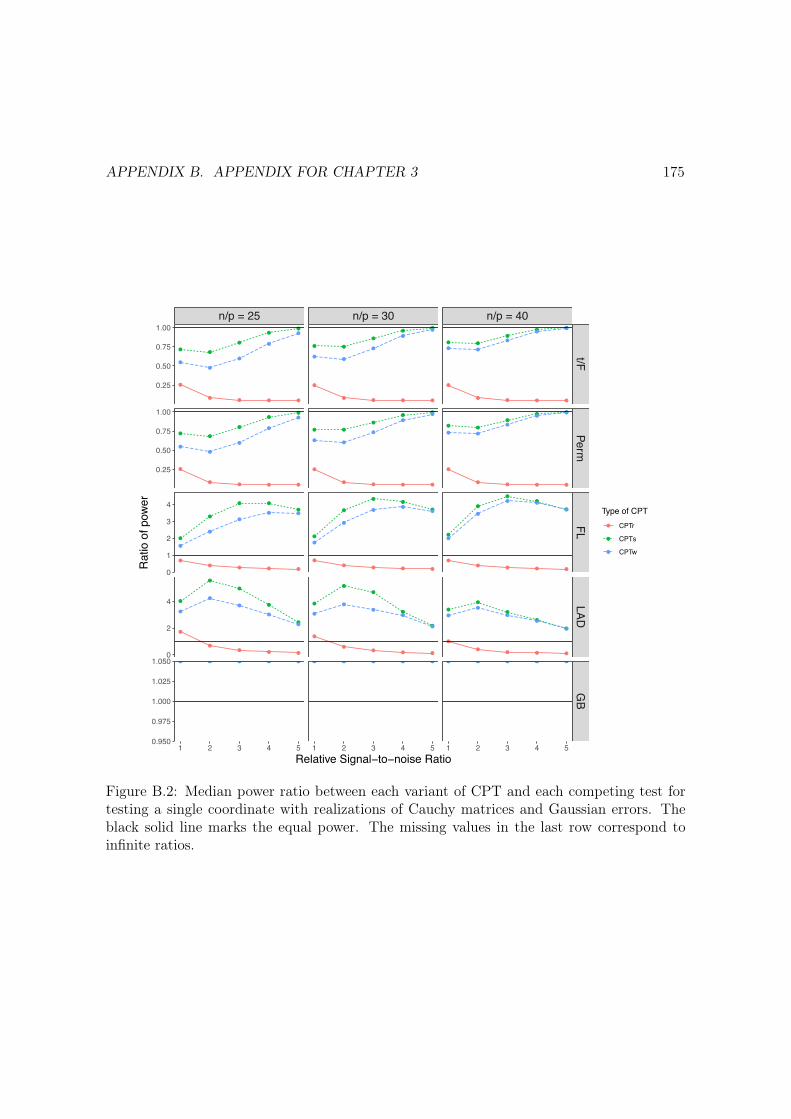
APPENDIX B. APPENDIX FOR CHAPTER 3 175
●
●
●
●
●
●
●
●
●
●
●
●
●
●●
●
●
●
●
●
●
●
●
●
●
●
●
●
●●
●
●
●
●
●
●
●
●
●
●
●
●
●
●●
●
●
●
●
●
●
●
●
●
●
●
●
●
●●
●●● ●●● ●●● ●●● ●●●
●
●
●
●
●
●
●
●
●
●
●
●
●
●●
●
●
●
●
●
●
●
●
●
●
●
●
●
●●
●
●
●
●
●
●
●
●
●
●
●
●
●
●●
●
●
●
●
●
●
●
●
●
●
●●
●
●●
●●● ●●● ●●● ●●● ●●●
●
●
●
●
●
●
●
●●
●
●●
●
●●
●
●
●
●
●
●
●
●●
●
●●
●
●●
●
●●
●
●
●
●
●●
●
●●
●
●●
●
●
●
●
●
●
●
●●
●
●●
●
●●
●●● ●●● ●●● ●●● ●●●
n/p = 25 n/p = 30 n/p = 40
t/FPerm
FLLAD
GB
1 2 3 4 5 1 2 3 4 5 1 2 3 4 5
0.25
0.50
0.75
1.00
0.25
0.50
0.75
1.00
0
1
2
3
4
0
2
4
0.950
0.975
1.000
1.025
1.050
Relative Signal−to−noise Ratio
Rat
io o
f pow
er
Type of CPT●
●
●
CPTr
CPTs
CPTw
Figure B.2: Median power ratio between each variant of CPT and each competing test fortesting a single coordinate with realizations of Cauchy matrices and Gaussian errors. Theblack solid line marks the equal power. The missing values in the last row correspond toinfinite ratios.
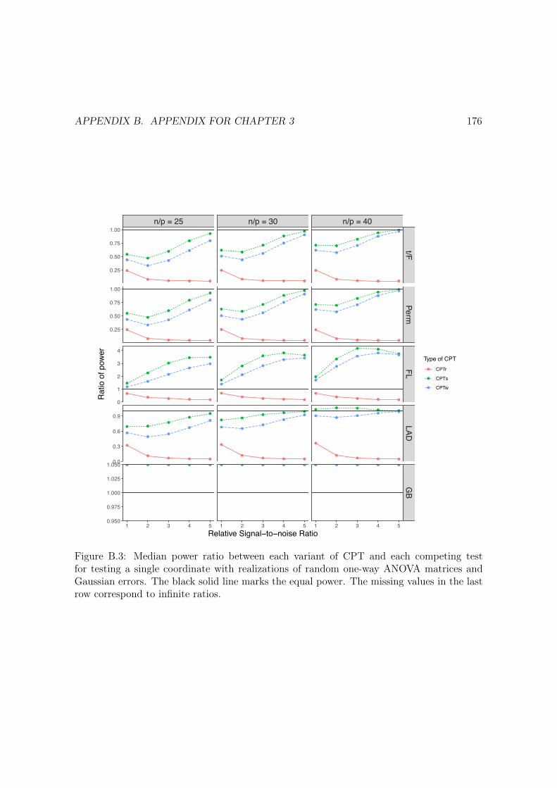
APPENDIX B. APPENDIX FOR CHAPTER 3 176
●
●
●
●
●
●
●
●
●
●
●
●
●
●
●
●
●
●
●
●
●
●
●
●
●
●
●
●
●
●
●
●
●
●
●
●
●
●
●
●
●
●
●
●
●
●
●
●
●
●
●
●
●
●
●
●
●
●
●
●
●●● ●●● ●●● ●●● ●●●
●
●
●
●
●
●
●
●
●
●
●
●
●
●
●
●
●
●
●
●
●
●
●
●
●
●
●
●
●
●
●
●
●
●
●
●
●
●
●
●
●
●
●
●●
●
●
●
●
●
●
●
●
●
●
●
●
●
●●
●●● ●●● ●●● ●●● ●●●
●
●
●
●
●
●
●
●
●
●
●
●
●
●●
●
●
●
●
●
●
●
●
●
●
●
●
●
●●
●
●●
●
●
●
●
●
●
●
●
●
●
●●
●
●
●
●
●
●
●
●
●
●
●●
●
●●
●●● ●●● ●●● ●●● ●●●
n/p = 25 n/p = 30 n/p = 40
t/FPerm
FLLAD
GB
1 2 3 4 5 1 2 3 4 5 1 2 3 4 5
0.25
0.50
0.75
1.00
0.25
0.50
0.75
1.00
0
1
2
3
4
0.0
0.3
0.6
0.9
0.950
0.975
1.000
1.025
1.050
Relative Signal−to−noise Ratio
Rat
io o
f pow
er
Type of CPT●
●
●
CPTr
CPTs
CPTw
Figure B.3: Median power ratio between each variant of CPT and each competing testfor testing a single coordinate with realizations of random one-way ANOVA matrices andGaussian errors. The black solid line marks the equal power. The missing values in the lastrow correspond to infinite ratios.

APPENDIX B. APPENDIX FOR CHAPTER 3 177
●
●
●
●
●
●
●
●
●
●
●
●
●
●
●
●
●
●
●
●
●
●
●
●
●
●
●
●
●●
●
●
●
●
●
●
●
●
●
●
●
●
●
●
●
●
●●●
●●
●
●●
●
●●
●
●●
●●● ●●● ●●● ●●● ●●●
●
●
●
●
●
●
●
●
●
●
●●
●
●●
●
●
●
●
●
●
●
●
●
●
●●
●
●●
●
●●
●
●
●
●
●
●
●
●
●
●
●
●
●
●●●
●●
●
●●
●
●●
●
●●
●●● ●●● ●●● ●●● ●●●
●
●
●
●
●
●
●
●●
●
●●
●
●●
●
●
●
●
●
●
●
●●
●
●●
●
●●
●
●●
●
●
●
●
●●
●
●●
●
●●
●
●●
●
●●
●
●●
●
●●
●
●●
●●● ●●● ●●● ●●● ●●●
n/p = 25 n/p = 30 n/p = 40
t/FPerm
FLLAD
GB
1 2 3 4 5 1 2 3 4 5 1 2 3 4 5
0.25
0.50
0.75
1.00
0.25
0.50
0.75
1.00
1
2
3
4
5
0.25
0.50
0.75
1.00
0.950
0.975
1.000
1.025
1.050
Relative Signal−to−noise Ratio
Rat
io o
f pow
er
Type of CPT●
●
●
CPTr
CPTs
CPTw
Figure B.4: Median power ratio between each variant of CPT and each competing testfor testing a single coordinate with realizations of random one-way ANOVA matrices andCauchy errors. The black solid line marks the equal power. The missing values in the lastrow correspond to infinite ratios.
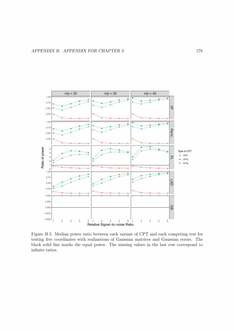
APPENDIX B. APPENDIX FOR CHAPTER 3 178
●
●
●
●
●
●
●
●
●
●
●
●
●
●
●
●
●
●
●
●
●
●
●
●
●
●
●
●
●
●
●
●
●
●
●
●
●
●
●
●
●
●
●
●
●
●
●
●
●
●
●
●
●
●
●
●
●
●
●
●
●●● ●●● ●●● ●●● ●●●
●
●
●
●
●
●
●
●
●
●
●
●
●
●●
●
●
●
●
●
●
●
●
●
●
●
●
●
●●
●
●
●
●
●
●
●
●
●
●
●
●
●
●●
●
●
●
●
●
●
●
●
●
●
●
●
●
●●
●●● ●●● ●●● ●●● ●●●
●
●
●
●
●
●
●
●
●
●
●●
●
●●
●
●
●
●
●
●
●
●
●
●
●●
●
●●
●
●
●
●
●
●
●
●
●
●
●●
●
●●
●
●
●
●
●
●
●
●
●
●
●●
●
●●
●●● ●●● ●●● ●●● ●●●
n/p = 25 n/p = 30 n/p = 40
t/FPerm
FLLAD
GB
1 2 3 4 5 1 2 3 4 5 1 2 3 4 5
0.25
0.50
0.75
1.00
0.25
0.50
0.75
1.00
0
1
2
3
4
5
0.25
0.50
0.75
1.00
0.950
0.975
1.000
1.025
1.050
Relative Signal−to−noise Ratio
Rat
io o
f pow
er
Type of CPT●
●
●
CPTr
CPTs
CPTw
Figure B.5: Median power ratio between each variant of CPT and each competing test fortesting five coordinates with realizations of Gaussian matrices and Gaussian errors. Theblack solid line marks the equal power. The missing values in the last row correspond toinfinite ratios.

APPENDIX B. APPENDIX FOR CHAPTER 3 179
●
●
●
●
●
●
●
●
●
●
●
●
●
●
●
●
●
●
●
●
●
●
●
●
●
●
●
●
●
●
●
●
●
●
●
●
●
●
●
●
●
●
●
●
●
●
●●
●
●
●
●
●
●
●
●
●
●
●
●
●●● ●●● ●●● ●●● ●●●
●
●
●
●
●
●
●
●
●
●
●
●
●
●
●
●
●
●
●
●
●
●
●
●
●
●
●
●
●
●
●
●
●
●
●
●
●
●
●
●
●
●
●
●
●
●
●●
●
●
●
●
●
●
●
●●
●
●●
●●● ●●● ●●● ●●● ●●●
●
●
●
●
●
●
●
●
●
●
●
●
●
●●
●
●
●
●
●
●
●
●
●
●
●
●
●
●●
●
●
●
●
●
●
●
●
●
●
●
●
●
●●
●
●●
●
●●
●
●●
●
●●
●
●●
●●● ●●● ●●● ●●● ●●●
n/p = 25 n/p = 30 n/p = 40
t/FPerm
FLLAD
GB
1 2 3 4 5 1 2 3 4 5 1 2 3 4 5
0.25
0.50
0.75
1.00
0.25
0.50
0.75
1.00
1
2
3
4
0.25
0.50
0.75
1.00
0.950
0.975
1.000
1.025
1.050
Relative Signal−to−noise Ratio
Rat
io o
f pow
er
Type of CPT●
●
●
CPTr
CPTs
CPTw
Figure B.6: Median power ratio between each variant of CPT and each competing test fortesting five coordinates with realizations of Gaussian matrices and Cauchy errors. The blacksolid line marks the equal power. The missing values in the last row correspond to infiniteratios.

APPENDIX B. APPENDIX FOR CHAPTER 3 180
●
●
●
●
●
●
●
●
●
●
●
●
●
●●
●
●
●
●
●
●
●
●
●
●
●
●
●
●●
●
●
●
●
●
●
●
●
●
●
●
●
●
●●
●
●
●
●
●
●
●
●
●
●
●
●
●
●
●
●●● ●●● ●●● ●●● ●●●
●
●
●
●
●
●
●
●●
●
●●
●
●●
●
●
●
●
●
●
●
●●
●
●●
●
●●
●
●
●
●
●
●
●
●●
●
●●
●
●●
●
●
●
●
●
●
●
●●
●
●●
●
●●
●●● ●●● ●●● ●●● ●●●
●
●
●
●
●●
●
●●
●
●●
●
●●
●
●●
●
●●
●
●●
●
●●
●
●●
●
●●
●
●●
●
●●
●
●●
●
●●
●
●●
●
●
●
●
●●
●
●●
●
●●
●●● ●●● ●●● ●●● ●●●
n/p = 25 n/p = 30 n/p = 40
t/FPerm
FLLAD
GB
1 2 3 4 5 1 2 3 4 5 1 2 3 4 5
0.00
0.25
0.50
0.75
1.00
1.25
0.00
0.25
0.50
0.75
1.00
1.25
0
2
4
6
0
2
4
6
0.950
0.975
1.000
1.025
1.050
Relative Signal−to−noise Ratio
Rat
io o
f pow
er
Type of CPT●
●
●
CPTr
CPTs
CPTw
Figure B.7: Median power ratio between each variant of CPT and each competing test fortesting five coordinates with realizations of Cauchy matrices and Gaussian errors. The blacksolid line marks the equal power. The missing values in the last row correspond to infiniteratios.

APPENDIX B. APPENDIX FOR CHAPTER 3 181
●
●
●
●
●
●
●
●
●
●
●●
●
●●
●
●
●
●
●
●
●
●●
●
●●
●
●●
●
●
●
●
●
●
●
●
●
●
●
●
●
●
●
●
●
●
●
●
●
●
●
●
●
●
●
●
●
●
●●● ●●● ●●● ●●● ●●●
●
●
●
●
●
●
●
●●
●
●●
●
●●
●
●
●
●
●●
●
●●
●
●●
●
●●
●
●
●
●
●
●
●
●
●
●
●
●
●
●●
●
●
●
●
●●
●
●●
●
●●
●
●●
●●● ●●● ●●● ●●● ●●●
●
●
●
●
●●
●
●●
●
●●
●
●●
●
●
●
●
●●
●
●●
●
●●
●
●●
●
●
●
●
●●
●
●●
●
●●
●
●●
●
●●
●
●●
●
●●
●
●●
●
●●
●●● ●●● ●●● ●●● ●●●
n/p = 25 n/p = 30 n/p = 40
t/FPerm
FLLAD
GB
1 2 3 4 5 1 2 3 4 5 1 2 3 4 5
0.0
0.5
1.0
1.5
2.0
0
1
2
5
10
0.25
0.50
0.75
1.00
0.950
0.975
1.000
1.025
1.050
Relative Signal−to−noise Ratio
Rat
io o
f pow
er
Type of CPT●
●
●
CPTr
CPTs
CPTw
Figure B.8: Median power ratio between each variant of CPT and each competing test fortesting five coordinates with realizations of Cauchy matrices and Cauchy errors. The blacksolid line marks the equal power. The missing values in the last row correspond to infiniteratios.

APPENDIX B. APPENDIX FOR CHAPTER 3 182
●
●●
●
●
●
●
●
●
●
●
●
●
●
●
●
●●
●
●
●
●
●
●
●
●
●
●
●
●
●
●●
●
●
●
●
●
●
●
●
●
●
●
●
●
●●
●
●
●
●
●
●
●
●
●
●
●
●
●●● ●●● ●●● ●●●
●
●
●
●
●
●
●
●
●
●
●
●
●
●
●
●
●●
●
●
●
●
●
●
●
●
●
●
●
●
●
●●
●
●
●
●
●
●
●
●
●
●
●
●
●
●
●
●
●●
●
●
●
●
●
●
●
●
●
●
●
●
●●● ●●● ●●● ●●●
●
●
●
●
●
●
●
●
●
●
●●
●
●●
●
●●
●
●●
●
●
●
●
●●
●
●●
●
●●
●
●●
●
●
●
●
●
●
●
●
●
●
●●
●
●
●
●
●
●
●
●●
●
●●
●
●●
●●● ●●● ●●● ●●●
●
●●
n/p = 25 n/p = 30 n/p = 40
t/FPerm
FLLAD
GB
1 2 3 4 5 1 2 3 4 5 1 2 3 4 5
0.25
0.50
0.75
1.00
0.25
0.50
0.75
1.00
1
2
3
0.25
0.50
0.75
1.00
0
10
20
30
Relative Signal−to−noise Ratio
Rat
io o
f pow
er
Type of CPT●
●
●
CPTr
CPTs
CPTw
Figure B.9: Median power ratio between each variant of CPT and each competing test fortesting five coordinates with realizations of random one-way ANOVA matrices and Gaussianerrors. The black solid line marks the equal power. The missing values in the last rowcorrespond to infinite ratios.

APPENDIX B. APPENDIX FOR CHAPTER 3 183
●
●●
●
●●
●
●●
●
●
●
●
●●
●
●
●
●
●
●
●
●
●
●
●
●
●
●
●
●
●●
●
●
●
●
●
●
●
●
●
●
●
●
●●● ●
●●●
●●
●
●●
●
●●
●●● ●●● ●●● ●●●
●
●
●
●
●●
●
●●
●
●●
●
●●
●
●●
●
●
●
●
●
●
●
●
●
●
●
●
●
●●
●
●●
●
●
●
●
●
●
●
●
●
●
●
●
●●● ●
●●●
●●
●
●●
●
●●
●●● ●●● ●●● ●●● ●●●
●
●●
●
●●
●
●●
●
●●
●
●●
●
●●
●
●●
●
●●
●
●●
●
●●
●
●●
●
●●
●
●●
●
●●
●
●●
●●● ●●●
●
●●
●
●●
●
●●
●●● ●●● ●●● ●●● ●●●
n/p = 25 n/p = 30 n/p = 40
t/FPerm
FLLAD
GB
1 2 3 4 5 1 2 3 4 5 1 2 3 4 5
0.25
0.50
0.75
1.00
0.25
0.50
0.75
1.00
1
2
3
0.25
0.50
0.75
1.00
3
6
9
Relative Signal−to−noise Ratio
Rat
io o
f pow
er
Type of CPT●
●
●
CPTr
CPTs
CPTw
Figure B.10: Median power ratio between each variant of CPT and each competing test fortesting five coordinates with realizations of random one-way ANOVA matrices and Cauchyerrors. The black solid line marks the equal power. The missing values in the last rowcorrespond to infinite ratios.
184
Appendix C
Appendix for Chapter 4
C.1 Concentration Inequalities for Sampling Without
Replacement
C.1.1 Some existing toolsThe proofs rely on concentration inequalities for sampling without replacement. Hoeffding(1963, Theorem 4) proved the following result that sampling without replacement is moreconcentrated in convex ordering than i.i.d. sampling.
Proposition C.1.1. Let C = (c1, . . . , cn) be a finite population of fixed elements. LetZ1, . . . , Zm be a random sample with replacement from C and W1, . . . ,Wm be a randomsample without replacement from C. If the function f(x) is continuous and convex, then
Ef
mX
i=1
Zi
!� Ef
mX
i=1
Wi
!.
From Proposition C.1.1, most concentration inequalities for independent sampling carryover to sampling without replacement. Later a line of works, in different contexts, showed aneven more surprising phenomenon that sampling without replacement can have strictly betterconcentration than independent sampling (e.g., Serfling 1974; Diaconis and Shahshahani1987; Lee and Yau 1998; Bobkov 2004; Cortes et al. 2009; El-Yaniv and Pechyony 2009;Bardenet and Maillard 2015; Tolstikhin 2017). In particular, Tolstikhin (2017, Theorem 9)proved a useful concentration inequality for the empirical processes for sampling withoutreplacement.
Proposition C.1.2. Let C = (c1, . . . , cn) be a finite population of fixed elements, andW1, . . . ,Wm be a random sample without replacement from C. Let F be a class of func-tions on C, and
S(F) = supf2F
mX
i=1
f(Wi), ⌫(F)2 = supf2F
Var(f(W1)).

APPENDIX C. APPENDIX FOR CHAPTER 4 185
ThenP(S(F)� E[S(F)] � t) exp
⇢� (n+ 2)t2
8n2⌫(F)2
�.
Proposition C.1.2 gives a sub-gaussian tail of S(F) with the sub-gaussian parameterdepending solely on the variance. In contrast, the concentration inequalities in the standardempirical process theory for independent sampling usually requires the functions in F to beuniformly bounded and the tail is either sub-gaussian with the sub-gaussian parameter beingthe uniform bound on F or sub-exponential with Bernstein-style behaviors; see Boucheronet al. (2013) for instance. Therefore, Proposition C.1.2 provides a more precise statementthat sampling without replacement is more concentrated than independent sampling for alarge class of statistics.
We need the following result from Tropp (2016, Theorem 5.1.(2)) to prove the matrixconcentration inequality.
Proposition C.1.3. Let V1, . . . , Vm be independent p⇥ p random matrices with EVi = 0 forall i. Let C(p) = 4(1 + d2 log pe). Then
0
@E�����
nX
i=1
Vi
�����
2
op
1
A
12
pC(p)
�����
nX
i=1
EV 2
i
�����
12
op
+ C(p)
✓E max
1in
kVik2op◆ 1
2
.
We will also use the facts that for any u 2 Rp and Hermitian V 2 Rp⇥p,
kuk2 = sup!2Sp�1
uT!, kV kop = sup!2Sp�1
!TV !.
C.1.2 Proofs of Lemmas 4.6.3 and 4.6.4Proof of Lemma 4.6.3. Let
C = (u1, . . . , un), and F = {f!(u) = uT! : ! 2 Sp�1}.
Let u be a vector that is randomly sampled from C. Then
⌫2(F) = sup!2Sp�1
Var(uT!) sup!2Sp�1
E(uT!)2
= sup!2Sp�1
1
n
nX
i=1
(uTi!)2 = sup
!2Sp�1
!T
1
n
nX
i=1
uiuTi
!!
= sup!2Sp�1
!T
✓UTU
n
◆!
kUk2op
n.
By Proposition C.1.2,
P �����
X
i2T
ui
�����2
� E�����X
i2T
ui
�����2
+ t
! exp
⇢�(n+ 2)t2
8nkUk2op
� exp
⇢� t2
8kUk2op
�,

APPENDIX C. APPENDIX FOR CHAPTER 4 186
or, equivalently, with probability 1� �,�����X
i2T
ui
�����2
E�����X
i2T
ui
�����2
+ kUkop
r8 log
1
�. (S1)
By the Cauchy–Schwarz inequality, E�����X
i2T
ui
�����2
!2
E�����X
i2T
ui
�����
2
2
=pX
j=1
E X
i2T
uij
!2
.
Lemma 4.6.1 implies
E X
i2T
uij
!2
=m(n�m)
n(n� 1)
nX
i=1
u2
ij.
As a result, E�����X
i2T
ui
�����2
!2
m(n�m)
n(n� 1)
nX
i=1
kuik22 = kUk2F
m(n�m)
n(n� 1). (S2)
We complete the proof by using (S1) and (S2).
Proof of Lemma 4.6.4. Let
C = (V1, . . . , Vn), and F = {f!(V ) = !TV ! : ! 2 Sp�1}.
Let V be a vector that is randomly sampled from C. Then
⌫2(F) = sup!2Sp�1
Var(!TV !) sup!2Sp�1
E(!TV !)2 = sup!2Sp�1
1
n
nX
i=1
(!TVi!)2 = ⌫2�.
By Proposition C.1.2,
P
0
@�����X
i2T
Vi
�����op
� E�����X
i2T
Vi
�����op
+ t
1
A exp
⇢�(n+ 2)t2
8n2⌫2�
� exp
⇢� t2
8n⌫2�
�,
or, equivalently, with probability 1� �,�����X
i2T
Vi
�����op
E�����X
i2T
Vi
�����op
+
r8n log
1
�⌫�. (S3)
We then bound E��P
i2T Vi
��op. Let V1, . . . , Vm be an i.i.d. random sample with replace-
ment from C. We have
E�����X
i2T
Vi
�����op
E�����
mX
i=1
Vi
�����op
0
@E�����
mX
i=1
Vi
�����
2
op
1
A
12
pnC(p)⌫ + C(p)⌫+, (S4)

APPENDIX C. APPENDIX FOR CHAPTER 4 187
where the first inequality follows from Proposition C.1.1 due to the convexity of k · kop,the second inequality follows from the Cauchy–Schwarz inequality, and the third inequalityfollows from Proposition C.1.3.
Combining (S3) and (S4), we complete the proof.
C.2 Mean and Variance of the Sum of Random Rows
and Columns of a Matrix
We give a full proof of Lemma 4.6.5. When m = 0 or m = n, QT is deterministic with zerovariance and the inequality holds automatically. Thus we assume 1 m n� 1.
LetP
[i1,...,ik]denote the sum over all (i1, . . . , ik) with mutually distinct elements in
{1, . . . , n}. For instance,P
[i,j]denotes the sum over all pairs (i, j) with i 6= j. We first
state a basic result for sampling without replacement.
Lemma C.2.1. Let i1, . . . , ik be distinct indices in {1, . . . , n} and T be a uniformly randomsubset of {1, . . . , n} with size m. Then
P (i1, . . . , ik 2 T ) =m · · · (m� k + 1)
n · · · (n� k + 1).
By definition,
QT =nX
i=1
QiiI(i 2 T ) +X
[i,j]
QijI(i, j 2 T ). (S5)
The mean of QT follows directly from Lemma C.2.1:
EQT =nX
i=1
Qii ·m
n+X
[i,j]
Qij ·m(m� 1)
n(n� 1)
=m(n�m)
n(n� 1)tr(Q) +
m(m� 1)
n(n� 1)(1TQ1).
The rest of this section proves the result of the variance. Let
c1 =m(n�m)
n(n� 1), c2 = Var (I(1, 2 2 T )) = c1
(m� 1)(n+m� 1)
n(n� 1),
c3 = Cov (I(1, 2 2 T ), I(1, 3 2 T )) = c1(m� 1)(mn� 2m� 2n+ 2)
n(n� 1)(n� 2),
c4 = Cov (I(1, 2 2 T ), I(3, 4 2 T )) = c1(m� 1)(�4mn+ 6n+ 6m� 6)
n(n� 1)(n� 2)(n� 3),
c5 = Cov (I(1 2 T ), I(1, 2 2 T )) = c1m� 1
n,
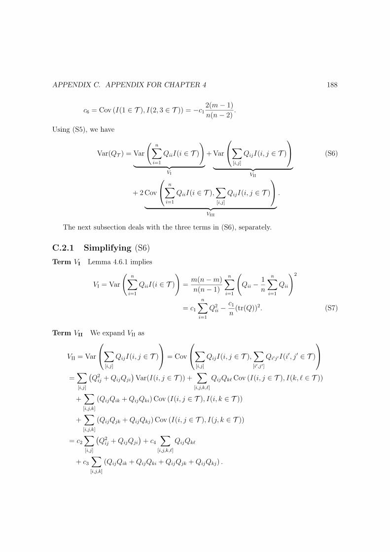
APPENDIX C. APPENDIX FOR CHAPTER 4 188
c6 = Cov (I(1 2 T ), I(2, 3 2 T )) = �c12(m� 1)
n(n� 2).
Using (S5), we have
Var(QT ) = Var
nX
i=1
QiiI(i 2 T )
!
| {z }VI
+Var
0
@X
[i,j]
QijI(i, j 2 T )
1
A
| {z }VII
(S6)
+ 2Cov
0
@nX
i=1
QiiI(i 2 T ),X
[i,j]
QijI(i, j 2 T )
1
A
| {z }VIII
.
The next subsection deals with the three terms in (S6), separately.
C.2.1 Simplifying (S6)Term VI Lemma 4.6.1 implies
VI = Var
nX
i=1
QiiI(i 2 T )
!=
m(n�m)
n(n� 1)
nX
i=1
Qii �
1
n
nX
i=1
Qii
!2
= c1
nX
i=1
Q2
ii� c1
n(tr(Q))2. (S7)
Term VII We expand VII as
VII = Var
0
@X
[i,j]
QijI(i, j 2 T )
1
A = Cov
0
@X
[i,j]
QijI(i, j 2 T ),X
[i0,j0]
Qi0j0I(i0, j0 2 T )
1
A
=X
[i,j]
�Q2
ij+QijQji
�Var(I(i, j 2 T )) +
X
[i,j,k,`]
QijQk`Cov (I(i, j 2 T ), I(k, ` 2 T ))
+X
[i,j,k]
(QijQik +QijQki) Cov (I(i, j 2 T ), I(i, k 2 T ))
+X
[i,j,k]
(QijQjk +QijQkj) Cov (I(i, j 2 T ), I(j, k 2 T ))
= c2X
[i,j]
�Q2
ij+QijQji
�+ c4
X
[i,j,k,`]
QijQk`
+ c3X
[i,j,k]
(QijQik +QijQki +QijQjk +QijQkj) .
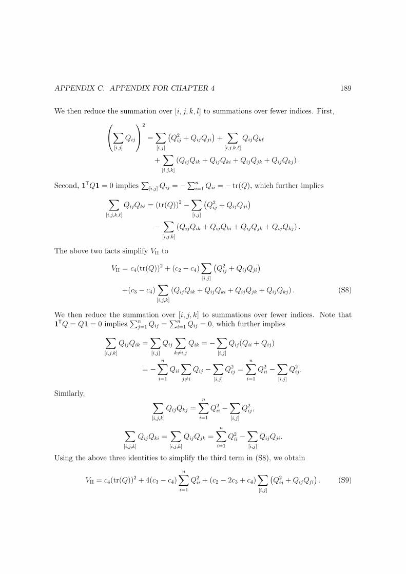
APPENDIX C. APPENDIX FOR CHAPTER 4 189
We then reduce the summation over [i, j, k, l] to summations over fewer indices. First,0
@X
[i,j]
Qij
1
A2
=X
[i,j]
�Q2
ij+QijQji
�+
X
[i,j,k,`]
QijQk`
+X
[i,j,k]
(QijQik +QijQki +QijQjk +QijQkj) .
Second, 1TQ1 = 0 impliesP
[i,j]Qij = �
Pn
i=1Qii = � tr(Q), which further implies
X
[i,j,k,`]
QijQk` = (tr(Q))2 �X
[i,j]
�Q2
ij+QijQji
�
�X
[i,j,k]
(QijQik +QijQki +QijQjk +QijQkj) .
The above two facts simplify VII to
VII = c4(tr(Q))2 + (c2 � c4)X
[i,j]
�Q2
ij+QijQji
�
+(c3 � c4)X
[i,j,k]
(QijQik +QijQki +QijQjk +QijQkj) . (S8)
We then reduce the summation over [i, j, k] to summations over fewer indices. Note that1TQ = Q1 = 0 implies
Pn
j=1Qij =
Pn
i=1Qij = 0, which further implies
X
[i,j,k]
QijQik =X
[i,j]
Qij
X
k 6=i,j
Qik = �X
[i,j]
Qij(Qii +Qij)
= �nX
i=1
Qii
X
j 6=i
Qij �X
[i,j]
Q2
ij=
nX
i=1
Q2
ii�X
[i,j]
Q2
ij.
Similarly,X
[i,j,k]
QijQkj =nX
i=1
Q2
ii�X
[i,j]
Q2
ij,
X
[i,j,k]
QijQki =X
[i,j,k]
QijQjk =nX
i=1
Q2
ii�X
[i,j]
QijQji.
Using the above three identities to simplify the third term in (S8), we obtain
VII = c4(tr(Q))2 + 4(c3 � c4)nX
i=1
Q2
ii+ (c2 � 2c3 + c4)
X
[i,j]
�Q2
ij+QijQji
�. (S9)
APPENDIX C. APPENDIX FOR CHAPTER 4 190
Term VIII The covariance term is
VIII = Cov
0
@nX
i=1
QiiI(i 2 T ),X
[i,j]
QijI(i, j 2 T )
1
A
=X
[i,j]
Qii(Qij +Qji) Cov (I(i 2 T ), I(i, j 2 T ))
+X
[i,j,k]
QiiQjk Cov (I(i 2 T ), I(j, k 2 T ))
= c5X
[i,j]
Qii(Qij +Qji) + c6X
[i,j,k]
QiiQjk.
Similar to previous arguments,
X
[i,j]
Qii(Qij +Qji) =nX
i=1
Qii
X
j 6=i
(Qij +Qji) = �2nX
i=1
Q2
ii,
X
[i,j,k]
QiiQjk =X
[i,j]
Qii
X
k 6=i,j
Qjk = �X
[i,j]
Qii(Qjj +Qji)
= �nX
i=1
Qii
X
j 6=i
(Qjj +Qji) = �nX
i=1
Qii (tr(Q)�Qii �Qii)
= �(tr(Q))2 + 2nX
i=1
Q2
ii.
Using the above two identities, we can simplify VIII to
VIII = �c6(tr(Q))2 � 2(c5 � c6)nX
i=1
Q2
ii. (S10)
Putting (S7), (S9) and (S10) together, we obtain that
Var(QT ) = (c1 + 4c3 � 4c4 � 4c5 + 4c6)| {z }CI
nX
i=1
Q2
ii+⇣c4 �
c1n
� 2c6⌘
| {z }CII
(tr(Q))2
+ (c2 � 2c3 + c4)| {z }CIII
X
[i,j]
(Q2
ij+QijQji). (S11)
We simplify (S11) in the next subsection by deriving bounds for the coefficients.

APPENDIX C. APPENDIX FOR CHAPTER 4 191
C.2.2 Bounding the coefficients CI, CII and CIII in (S11)Bounding CI We have
CI = c1 + 4c3 � 4c4 � 4c5 + 4c6
=c1 + 4c1m� 1
n
✓mn� 2m� 2n+ 2
(n� 1)(n� 2)+
4mn� 6m� 6n+ 6
(n� 1)(n� 2)(n� 3)� 1� 2
n� 2
◆.
Through tedious calculation, we obtain that
mn� 2m� 2n+ 2
(n� 1)(n� 2)+
4mn� 6m� 6n+ 6
(n� 1)(n� 2)(n� 3)� 1� 2
n� 2= � (n�m� 1)n
(n� 2)(n� 3).
Thus, CI = c1⇣1� 4(m�1)(n�m�1)
(n�2)(n�3)
⌘.
Bounding CII We have
CII = c4 �c1n
� 2c6 = �c1n
+ c1m� 1
n(n� 2)
✓�4mn+ 6m+ 6n� 6
(n� 1)(n� 3)+ 4
◆
=� c1n
+ c1(m� 1)(4n2 � 4mn+ 6m� 10n+ 6)
n(n� 1)(n� 2)(n� 3)
=� c1n
✓1� (m� 1)(n�m� 1)(4n� 6)
(n� 1)(n� 2)(n� 3)
◆
c1(m� 1)(n�m� 1)(4n� 6)
n(n� 1)(n� 2)(n� 3) c1
n
4(m� 1)(n�m� 1)
n(n� 2)(n� 3).
Bounding CIII We consider four cases.• If m = 1, then c2 = c3 = c4 = 0 and CIII c1
2.
• If m = 2, then
CIII = c1
✓n+ 1
n(n� 1)� �4
n(n� 1)(n� 2)� 2
n(n� 1)(n� 2)
◆
= c1
✓n+ 1
n(n� 1)+
2
n(n� 1)(n� 2)
◆ c1
2.
• If m = 3, then
CIII = c1
✓2(n+ 2)
n(n� 1)� 4(n� 4)
n(n� 1)(n� 2)� 12n� 24
n(n� 1)(n� 2)(n� 3)
◆
= c1
✓2(n+ 2)
n(n� 1)� 4(n� 4)
n(n� 1)(n� 2)� 12
n(n� 1)(n� 3)
◆.

APPENDIX C. APPENDIX FOR CHAPTER 4 192
If n � 7,
CIII c12(n+ 2)
n(n� 1) c1
2.
For n = 4, 5, 6, we can also verify that CIII c12.
• If m � 4, then
4mn� 6m� 6n+ 6 = (2m� 6)(n� 3) + 2(mn� 6) � (2m+ 2)(n� 3).
and thusc4 c1
(2m+ 2)(m� 1)
n(n� 1)(n� 2).
Then we have
CIII c1m� 1
n(n� 1)
✓n+m� 1� 2(mn� 2m� 2n+ 2)
n� 2� 2m+ 2
n� 2
◆
= c1m� 1
n(n� 1)
✓n+m� 1� 2mn� 4n� 2m+ 6
n� 2
◆
= c1m� 1
n(n� 1)
✓n�m+ 3� 2m� 2
n� 2
◆
c1
✓(m� 1)(n�m+ 3)
n(n� 1)� 2(m� 1)2
n(n� 1)(n� 2)
◆
c1
✓(n+ 2)2
4n(n� 1)� 2(m� 1)2
n(n� 1)(n� 2)
◆
c1
✓(n+ 2)2
4n(n� 1)� 18
n(n� 1)(n� 2)
◆. (S12)
If n � 7,
CIII c1(n+ 2)2
4n(n� 1) 81c1
168 c1
2.
For n = 4, 5, 6, we can also verify that CIII c12.
Therefore, we always have CIII c12.
Using the above bounds for (CI, CII, CIII) in (S11), we obtain that
Var (QT ) c1
✓1� 4(m� 1)(n�m� 1)
(n� 2)(n� 3)
◆ nX
i=1
Q2
ii
+ c14(m� 1)(n�m� 1)
(n� 2)(n� 3)
(tr(Q))2
n+
c12
X
[i,j]
(Q2
ij+QijQji).
Because (tr(Q))2 nP
n
i=1Q2
iiand QijQji (Q2
ij+ Q2
ji)/2, we conclude that Var (QT )
c1kQk2F.

APPENDIX C. APPENDIX FOR CHAPTER 4 193
C.3 Proofs of the Lemmas in Section 6.2
Proof of Lemma 4.6.6. Using the definitions of �2
nand ⇢e, we have
�2
n=
✓1
n1
� 1
n
◆ nX
i=1
e2i(1) +
✓1
n0
� 1
n
◆ nX
i=1
e2i(0) +
2
n
nX
i=1
ei(1)ei(0)
=n0
n1n
nX
i=1
e2i(1) +
n1
n0n
nX
i=1
e2i(0) +
2⇢en
vuutnX
i=1
e2i(1)
vuutnX
i=1
e2i(0).
If ⇢e � 0, then
�2
n� n0
n1n
nX
i=1
e2i(1) +
n1
n0n
nX
i=1
e2i(0) � min
⇢n1
n0
,n0
n1
�E2.
If ⇢e < 0, then using the fact✓r
n0
n1
a�r
n1
n0
b
◆2
� 0 () 2ab n0
n1
a2 +n1
n0
b2,
we obtain that
�2
n� (1 + ⇢e)
n0
n1n
nX
i=1
e2i(1) +
n1
n0n
nX
i=1
e2i(0)
!� ⌘min
⇢n1
n0
,n0
n1
�E2.
Putting the pieces together, we complete the proof.
Proof of Lemma 4.6.7. Recall that µt is the intercept from the OLS fit of Y obs
ton 1 and
Xt. From the Frisch–Waugh Theorem, it is identical to the coefficient of the OLS fit of theresidual (I �Ht)Y obs
ton the residual (I �Ht)1, after projecting onto Xt:
µt =1T(I �Ht)T(I �Ht)Y obs
t
k(I �Ht)1k22=
1T(I �Ht)Y obs
t
1T(I �Ht)1.
Using the definition (4.6) and the fact that (I �Ht)Xt = 0, we have
(I �Ht)Yobs
t= (I �Ht)(µt1 +Xt�t + et(t)) = µt(I �Ht)1 + (I �Ht)et(t),
=) µt = µt +1T(I �Ht)et(t)
1T(I �Ht)1= µt +
1Tet(t)/nt � 1THtet(t)/nt
1� 1THt1/nt
.
Recalling that ⌧ = µ1 � µ0, we complete the proof.

APPENDIX C. APPENDIX FOR CHAPTER 4 194
Proof of Lemma 4.6.8. Because kUkop kUkF , Lemma 4.6.3 implies that with probability1� �, �����
X
i2T
ui
�����2
.kUkF
sm(n�m)
n(n� 1)+
r8 log
1
�,
which further implies��P
i2T ui
��2= OP (kUkF ) . This immediately implies the three results
in Lemma 4.6.8 by choosing appropriate U.Let ui = ei(t) with
Pn
i=1ui = 0, U = (u1, . . . , un)T 2 Rn⇥1, and kUk2
F=
Pn
i=1u2
i=P
n
i=1e2i(t). Therefore,
1Tet(t) =
�����X
i2Tt
ui
�����2
= OP(kUkF ) = OP
0
@
vuutnX
i=1
e2i(t)
1
A = OP
⇣pnE2
⌘.
Let ui = xi withP
n
i=1ui = 0, U = X, and kUkF = kXkF =
ptr(XTX) = tr(nI) = np.
Therefore,
kXTt1k2 =
�����X
i2Tt
ui
�����2
= OP (kUkF ) = OP (pnp) .
Let ui = xiei(t) withP
n
i=1ui = 0 due to (4.7). Therefore,
kXTtet(t)k2 =
�����X
i2Tt
ui
�����2
= OP
0
@
vuutnX
i=1
kxik2e2i (t)
1
A .
Recalling (4.30) that kxik22 = nHii n, we have kXTtet(t)k2 = OP
�npE2
�.
We need the following proposition to prove Lemma 4.6.9.
Proposition C.3.1. A and B are two symmetric matrices. A is positive definite, and A+Bis invertible. Then
k(A+B)�1 � A�1kop kA�1k2
op· kBkop
1�min{1, kA�1kop · kBkop}.
Proof of Proposition C.3.1. Let M = A� 12BA� 1
2 and ⇤(M) be its spectrum. By definition,kMkop kA�1kop · kBkop. If kA�1kop · kBkop � 1, the inequality is trivial because the right-hand side of it is 1. Without loss of generality, we assume kA�1kop · kBkop < 1, whichimplies kMkop < 1.
Proposition C.3.1 follows by combining
k(A+B)�1 � A�1kop = kA� 12 ((I +M)�1 � I)A� 1
2kop
APPENDIX C. APPENDIX FOR CHAPTER 4 195
kA�1kop · kI � (I +M)�1kop
andkI � (I +M)�1kop sup
�2⇤(M)
�����
1 + �
���� =kMkop
1� kMkop kA�1kop · kBkop
1� kA�1kop · kBkop.
Proof of Lemma 4.6.9. Let Vi = xixTi � I, thenP
n
i=1Vi = 0. In the following, we will
repeatedly use the basic facts: n�1XTX = I, kxik22 = nHii, andP
n
i=1xixTi = XXT = nH.
Recalling the definitions of ⌫, ⌫+ and ⌫� in Lemma 4.6.4, we have
⌫2 =
�����1
n
nX
i=1
V 2
i
�����op
=
�����1
n
nX
i=1
�kxik22xix
Ti� 2xix
Ti+ I
������op
=
�����
1
n
nX
i=1
kxik22xixTi
!� I
�����op
=
�����
nX
i=1
HiixixTi
!� I
�����op
�����
nX
i=1
HiixixTi
�����op
+ 1
�����
nX
i=1
xixTi
�����op
+ 1 = nkHkop + 1 = n+ 1,
⌫+ = max1in
kxixTi� Ikop max
1in
kxik22 + 1 = n max1in
Hii + 1 = n+ 1,
⌫2� = sup!2Sp�1
1
n
nX
i=1
(!TVi!)2 = sup
!2Sp�1
1
n
nX
i=1
((xTi!)2 � 1)2
= sup!2Sp�1
1
n
nX
i=1
⇥(xT
i!)4 � 2(xT
i!)2 + 1
⇤
= sup!2Sp�1
1
n
nX
i=1
(xTi!)4 � 2!T
✓XTX
n
◆! + 1
= sup!2Sp�1
1
n
nX
i=1
(xTi!)4 � 1 sup
!2Sp�1
1
n
nX
i=1
(xTi!)4
sup!2Sp�1
1
n
nX
i=1
kxik22(xTi !)2 =
�����
nX
i=1
HiixixTi
�����op
n.
By Lemma 4.6.4,
k⌃t � Ikop
=1
nt
�����X
i2Tt
Vi
�����op
=OP
✓1
nt
hnpC(p)+ nC(p)+ n
pi◆
=OP
⇣p log p+ log p
⌘.

APPENDIX C. APPENDIX FOR CHAPTER 4 196
By Assumption 2, log p = o(1), and therefore the first result holds:
k⌃t � Ikop
= OP
⇣p log p
⌘= oP(1). (S13)
Thus with probability 1� o(1),
k⌃t � Ikop
1
2=) k⌃tkop � 1
2, (S14)
where we use the convexity of k · kop. Note that for any Hermitian matrix A, kA�1kop =�min(A)�1 where �min denotes the minimum eigenvalue. Thus with probability 1� o(1),
��⌃�1
t
��op
2. (S15)
Therefore, the second result holds:��⌃�1
t
��op
= OP(1).To prove the third result, we apply Proposition C.3.1 with A = I and B = ⌃t � I. By
(S14) and (S15), with probability 1 � o(1), A + B is invertible and kBkop 1/2. Togetherwith (S13), we have
��⌃�1
t� I
��op
= OP
✓kBkop
1� kBkop
◆= OP(kBkop) = OP(
p log p).
Proof of Lemma 4.6.10. First, (4.7) implies
1TQ(t) = 1TH diag(e(t)) = 1TX(XTX)�1XT diag(e(t)) = 0,
Q(t)1 = H diag(e(t))1 = He(t) = X(XTX)�1XTe(t) = 0,
which further imply 1TQ(t)1 = 0. Second, (4.9) implies tr(Q(t)) = n�t. Third,
kQ(t)k2F=
nX
i=1
nX
j=1
H2
ije2j(t) =
nX
j=1
e2j(t)
nX
i=1
H2
ij
!.
Because H is idempotent, HTH = H =)P
n
i=1H2
ij= Hjj for all j. Thus, kQ(t)k2
F=P
n
j=1e2j(t)Hjj nE2.
C.4 Proof of Proposition 4.3.1
C.4.1 Preparatory lemmasThe proofs rely on the following results.

APPENDIX C. APPENDIX FOR CHAPTER 4 197
Proposition C.4.1. [modified version of Corollary 3.1 of Yaskov (2014)] Let Zi be i.i.d.random vectors in Rp with mean 0 and covariance I. Suppose
L(�) , sup⌫2Sp�1
E|⌫TZi|� < 1
for some � > 2. For any constant C > 0, with probability 1� e�Cp,
�min
✓ZTZ
n
◆� 1� 5
✓pC
n
◆ ��+2
L(�)2
�+2
✓1 +
1
C
◆.
Proof of Proposition C.4.1. Write y = p/n and L = L(�). The proof of Corollary 3.1 ofYaskov (2014, page 6) showed that for any a > 0,
P✓�min
✓ZTZ
n
◆< 1� 4La��/2 � 5ay
◆ exp
��La�1��/2n
.
Let a = (Cy/L)�2/(�+2). Then the right-hand side is 1�e�Cp. Thus with probability 1�e�Cp,
�min
✓ZTZ
n
◆� 1� y
��+2L
2�+2
⇣5C� 2
�+2 + 4C�
�+2
⌘
� 1� 5 (Cy)�
�+2 L2
�+2
✓1 +
1
C
◆.
Proposition C.4.2 (Theorem 1 of Tikhomirov (2017)). Let Zi be i.i.d. random vectors inRp with mean 0 and covariance I. Suppose
L(�) , sup⌫2Sp�1
E|⌫TZi|� < 1
for some � > 2. Then with probability at least 1� 1/n,
⌫(�)�1
����ZTZ
n� I
����op
max1in kZik22n
+ L(�)2�
(⇣pn
⌘ ��2�
log4✓n
p
◆+⇣pn
⌘min{��2,2}min{�,4}
),
for some constant ⌫(�) depending only on �.
Proposition C.4.3 (Theorem 2 of Bahr and Esseen (1965)). Let Zi be independent mean-zero random variables. Then for any r 2 [1, 2),
E����
nX
i=1
Zi
����r
2nX
i=1
E|Zi|r.

APPENDIX C. APPENDIX FOR CHAPTER 4 198
C.4.2 A lemmaFirst we prove a more general result.
Lemma C.4.4. Let Zi be i.i.d. random vectors in Rp with mean µ 2 Rp and covariancematrix ⌃ 2 Rp⇥p. Let Zi = ⌃�1/2(Zi � µ), and assume
sup⌫2Sp�1
E|⌫TZi|� = O(1), and max1in
��kZik22 � EkZik22�� = OP(!(n, p)),
for some � > 2 and some function !(n, p) increasing in n and p. Let Z = (ZT1, . . . , ZT
n)T
and X = VZ so that X has centered columns. If p = O(n�) for some � < 1, then over therandomness of Z,
=p
n+OP
!(n, p)
n+⇣pn
⌘ 2��2�
log4✓n
p
◆+⇣pn
⌘min{2��2,6}min{�,4}
!.
Proof of Lemma C.4.4. Let Z = (ZT1, . . . , Zn)T and X = VZ. Then X = V
�Z � 1µT
�⌃� 1
2 =
VZ⌃� 12 , and thus
X(XTX)�1XT = VZ�ZTVZ
��1
ZTV = X(XTX)�1XT.
Therefore, we can assume µ = 0 and ⌃ = I without loss of generality, in which case Zi = Zi
has mean 0 and covariance matrix I.By definition, Hii = xT
i(XTX)�1xi, and therefore
Hii =1
nxTi
✓XTX
n
◆�1
� I
!xi +
kxik22n
kxik22n
0
@1 +
�����
✓XTX
n
◆�1
� I
�����op
1
A . (S16)
To bound , we need to bound two key terms below.
Bounding����n�1XTX
��1 � I���op
Let Z = n�1P
n
i=1Zi. Note that
EkZk22=
1
n2
nX
i=1
EkZik22 =1
nEkZ1k22 =
p
n.
By Markov’s inequality,kZk2
2= OP
⇣pn
⌘, (S17)

APPENDIX C. APPENDIX FOR CHAPTER 4 199
and more precisely,
P✓kZk2
2r
p
n
◆= 1� P
✓kZk2
2>
rp
n
◆� 1�
rp
n. (S18)
Let A1 denote the above event that kZk22pp/n. Then P(A1) � 1�
pp/n.
By Proposition C.4.2,����ZTZ
n� I
����op
= OP
max1in kZik22
n+⇣pn
⌘ ��2�
log4✓n
p
◆+⇣pn
⌘min{��2,2}min{�,4}
!.
By the condition of Lemma C.4.4,
max1in kZik22n
=p
n+ max
1in
kZik22 � EkZik22n
=p
n+OP
✓!(n, p)
n
◆. (S19)
Combining the above three equations, we have����XTX
n� I
����op
=
����ZTZ
n� I � ZZT
����op
����ZTZ
n� I
����op
+ kZk22
=OP
p
n+!(n, p)
n+⇣pn
⌘ ��2�
log4✓n
p
◆+⇣pn
⌘min{��2,2}min{�,4}
!
=OP
!(n, p)
n+⇣pn
⌘ ��2�
log4✓n
p
◆+⇣pn
⌘min{��2,2}min{�,4}
!, (S20)
where the last line uses the fact that the third term dominates the first term due to p/n ! 0.On the other hand, by Proposition C.4.1 with C =
pn/p, with probability 1� e�
pnp,
�min
✓ZTZ
n
◆� 1� 5
✓rp
n
◆ ��+2
L(�)2
�+2
✓1 +
rp
n
◆
� 1� 10⇣pn
⌘ �2(�+2)
L(�)2
�+2 . (S21)
Let A2 denote the event in (S21). Then P(A2) � 1� e�pnp.
Note that for any Hermitian matrices A and B, the convexity of k · kop implies that
|�min(A)� �min(B)| = |�max(�A)� �max(�B)| k � A� (�B)kop = kA� Bkop.
We have
�min
✓XTX
n
◆� �min
✓ZTZ
n
◆� kZZTkop = �min
✓ZTZ
n
◆� kZk2
2.

APPENDIX C. APPENDIX FOR CHAPTER 4 200
Let A = A1 [A2. Then on A,
�min
✓XTX
n
◆� 1� 10
⇣pn
⌘ �2(�+2)
L(�)2
�+2 �r
p
n.
Since p/n ! 0, for sufficiently large n,
�min
✓XTX
n
◆� 1
2
with probability
P(A) � P(A1) + P(A2)� 1 � 1� e�pnpL(�) �
rp
n= 1� o(1).
Finally, using Proposition C.3.1 with A = I and B = n�1XTX � I, by Slusky’s lemma,we have that
�����
✓XTX
n
◆�1
� I
�����op
= OP
!(n, p)
n+⇣pn
⌘ ��2�
log4✓n
p
◆+⇣pn
⌘min{��2,2}min{�,4}
!. (S22)
Because p = O(n�) for some � < 1,�����
✓XTX
n
◆�1
� I
�����op
= OP
✓!(n, p)
n
◆+ oP(1). (S23)
Bounding max1in kxik22 Because xi = Zi � Z, the Cauchy–Schwarz inequality implies
kxik22 = kZik22 � 2ZTiZ + kZk2
2 kZik22 + 2kZik2kZk2 + kZk2
2.
By (S19) and (S17),
max1in kxik22n
=EkZik22
n+
maxi kZik22 � EkZik22 + 2kZik2kZk2 + kZk22
n
=p
n+OP
!(n, p)
n+
r(p+ !(n, p))p
n3+
p
n2
!
=p
n+OP
!(n, p)
n+
r!(n, p)p
n3+
p
n3/2
!.
Because !(n, p) is increasing and p/n ! 0, we haver!(n, p)p
n3= O
✓!(n, p)
n
⇣pn
⌘1/2◆
= o
✓!(n, p)
n
◆.

APPENDIX C. APPENDIX FOR CHAPTER 4 201
Thus, we obtain that
max1in kxik22n
=p
n+OP
✓!(n, p)
n+
p
n3/2
◆. (S24)
Putting (S16), (S23) and (S24) together and using some tedious cancellations, we have
=p
n+OP
✓!(n, p)
n+
p
n3/2
◆
+OP
!2(n, p)
n2+⇣pn
⌘1+��2�
log4✓n
p
◆+⇣pn
⌘1+min{��2,2}min{�,4}
!. (S25)
Because ⇣pn
⌘1+min{��2,2}min{�,4} �
⇣pn
⌘3/2
� p
n3/2,
(S25) further simplifies to
=p
n+OP
!(n, p)
n+!2(n, p)
n2+⇣pn
⌘ 2��2�
log4✓n
p
◆+⇣pn
⌘min{2��2,6}min{�,4}
!
=p
n+OP
!(n, p)
nmax
⇢!(n, p)
n, 1
�+⇣pn
⌘ 2��2�
log4✓n
p
◆+⇣pn
⌘min{2��2,6}min{�,4}
!.
We complete the proof using 1.
C.4.3 Use Lemma C.4.4 to prove Proposition 4.3.1We have argued in the proof of Proposition C.4.4 that we can assume µ = 0 without lossof generality. Because the hat matrix is invariant to rescaling, we further assume EZ2
ij= 1
without loss of generality. Based on Proposition C.4.4, it suffices to verify
sup⌫2Sp�1
E|⌫TZi|� = O(1), (S26)
max1in
��kZik22 � EkZik22�� = OP
⇣n
2� p
2min{�,4}
⌘. (S27)
If (S26) and (S27) hold, by Proposition C.4.4, we have that
=p
n+OP
p2/min{�,4}
n(��2)/�+⇣pn
⌘ 2��2�
log4✓n
p
◆+⇣pn
⌘min{2��2,6}min{�,4}
!.
Then we can prove Proposition 4.3.1 for two cases.

APPENDIX C. APPENDIX FOR CHAPTER 4 202
Case 1 If � > 4, then 2��2
�< 3
2= min{2��2,6}
min{�,4} . Thus the third term dominates the secondterm in the above OP(·), implying
=p
n+OP
✓p1/2
n(��2)/�+⇣pn
⌘ 32
◆.
Case 2 If � 4, then
=p
n+OP
✓p2/�
n(��2)/�+⇣pn
⌘ 2��2�
log4✓n
p
◆◆.
Because ⇣pn
⌘ 2��2�
=p2/�
n(��2)/�
p(2��4)/�
n p2/�
n(��2)/�
p
n,
the first term dominates in the above OP(·), implying
=p
n+OP
✓p2/�
n(��2)/�
◆=
p
n+OP
✓p2/�
n(��2)/�+⇣pn
⌘3/2◆.
The last identity holds because p3/2/n3/2 is of smaller order and thus we can add it back.We will prove (S26) and (S27) below.
Proving (S26)
By Rosenthal (1970)’s inequality,
E|⌫TZi|� = E����
pX
j=1
⌫jZij
�����
C
0
@pX
j=1
|⌫j|�E|Zij|� +
pX
j=1
⌫2jEZ2
ij
!�/21
A
where C is a constant depending only on �. Because k⌫k2 = 1, we have max1jp |⌫j| 1and thus
pX
j=1
|⌫j|�E|Zij|� MpX
j=1
|⌫j|� MpX
j=1
|⌫j|� = M.
Hölder’s inequality implies EZ2
ij�E|Zij|�
�2/� M2/�, which further implies
pX
j=1
⌫2jEZ2
ij
!�/2
�M2/�
��/2= M.
Because the above two bounds hold regardless of ⌫, we conclude that
sup⌫2Sp�1
E|⌫TZi|� 2CM = O(1).

APPENDIX C. APPENDIX FOR CHAPTER 4 203
Proving (S27)
Let Wij = Z2
ij�EZ2
ij. Using Jensen’s inequality that E|(X +Y )/2|r (E|X|r +E|Y |r)/2 for
any random variables X, Y and r > 1, we obtain that
E|Wij|�/2 2�/2�1�E|Zij|� + (EZ2
ij)�/2
� 2�/2E|Zij|� 2�/2M , M.
We consider two cases.
Case 1: � � 4 By Hölder’s inequality, EW 2
ij M4/�. By Rosenthal (1970)’s inequality,
E|kZik22 � EkZik22|�/2 = E����
pX
j=1
Wij
�����/2
C
0
@pX
j=1
E|Wij|�/2 +
pX
j=1
EW 2
ij
!�/41
A
C⇣pM + p�/4M
⌘ CMp�/4,
which implies E��kZik22 � EkZik22
���/2 = O�p�/4
�. As a result,
E⇢max1in
��kZik22 � EkZik22���/2
�
nX
i=1
E��kZik22 � EkZik22
���/2 = O�np�/4
�.
By Markov’s inequality, max1in
��kZik22 � EkZik22�� = OP
�n2/�p1/2
�.
Case 2: � < 4 By Proposition C.4.3, with �/2 2 (1, 2),
E|kZik22 � EkZik22|�/2 = E����
pX
j=1
Wij
�����/2
2pX
j=1
E|Wij|�/2 2pM.
Similar to Case 1, max1in
��kZik22 � EkZik22�� = OP
�n2/�p2/�
�.
C.5 Proof of Proposition 4.3.2
Let Y (t) = n�1P
n
i=1Yi(t). Note that H1 = X(XTX)�1XT1 = 0. By definition, e(t) =
(I � H){Y (t) � Y (t)1} = (I � H){Y (t) � EYi(t)1}. Throughout the rest of the proof, weassume that EYi(t) = 0 without loss of generality, and define M(�) , maxt=0,1 E|Yi(t)|�.
C.5.1 Bounding E2Let Zi = Yi(t)2. Then the moment condition reads E|Zi|�/2 < 1. The Kolmogorov–Marcinkiewicz–Zygmund strong law of large number (Kallenberg 2006, Theorem 4.23) im-plies
1
n
nX
i=1
Zi
a.s.! EZ1 = OP(1), if � � 2,

APPENDIX C. APPENDIX FOR CHAPTER 4 204
1
n2/�
nX
i=1
Zi = o(1) =) 1
n
nX
i=1
Zi = oP(n2/��1), if � < 2.
On the other hand,
1
nke(t)k2
2=
1
nY (t)T(I �H)Y (t) 1
nkY (t)k2
2=
1
n
nX
i=1
Zi,
which further implies the bound for E2.
C.5.2 Bounding E�12
Without loss of generality, we assume that Yi(1) is not a constant with probability 1. Firstwe show that
Y (1)THY (1)
Y (1)TY (1)= oP(1).
For any permutation ⇡ on {1, . . . , n}, let H(⇡) denote the matrix with
H(⇡)ij = H⇡(i),⇡(j).
Because the Yi(1)’s are i.i.d., for any ⇡,
(Y1(1), . . . , Yn(1))d= (Y⇡�1(1)(1), . . . , Y⇡�1(n)(1)),
and thus
Y (1)TH(⇡)Y (1)
Y (1)TY (1)=
Pn
i=1
Pn
j=1H⇡(i),⇡(j)Yi(1)Yj(1)Pn
i=1Yi(1)2
=
Pn
i=1
Pn
j=1Hi,jY⇡�1(i)(1)Y⇡�1(j)(1)Pn
i=1Y⇡�1(i)(1)2
d=
Y (1)THY (1)
Y (1)TY (1).
Furthermore,Y (1)THY (1)
Y (1)TY (1) 1
and thus it has finite expectation. This implies that
EY (1)THY (1)
Y (1)TY (1)=
1
n!
X
⇡
Y (1)TH(⇡)Y (1)
Y (1)TY (1)=
1
n!
Y (1)TH⇤Y (1)
Y (1)TY (1),
where H⇤ =P
⇡H(⇡)/n! with the summation over all possible permutations. We can show
that
H⇤ii=
1
n
nX
i=1
Hii =p
n, H⇤
ij=
1
n(n� 1)
X
i 6=j
Hij = � 1
n(n� 1)
nX
i=1
Hii = � p
n(n� 1),

APPENDIX C. APPENDIX FOR CHAPTER 4 205
where the last equality uses the fact thatP
n
i=1
Pn
j=1Hij = 0. Therefore,
EY (1)THY (1)
Y (1)TY (1)= EY (1)TH⇤Y (1)
Y (1)TY (1)
=Ep
nY (1)TY (1)� p
n(n�1)
Pi 6=j
Yi(1)Yj(1)
Y (1)TY (1)
=p
n� 1� p
n(n� 1)E(P
n
i=1Yi(1))2
Y (1)TY (1) p
n� 1.
By Markov’s inequality, with probability 1� 2p
n�1= 1� o(1),
Y (1)THY (1)
Y (1)TY (1) 1
2.
Let A denote this event. ThenP(Ac) = o(1),
and on A,1
nke(1)k2
2=
1
nY (1)T(I �H)Y (1) � 1
2nkY (1)k2
2.
On the other hand, fix k > 0, and let Zi = Yi(1)I(|Yi(1)| k). For sufficiently large k,EZi > 0. By the law of large numbers, n�1
Pn
i=1Zi = EZi ⇥ (1 + oP(1)). Thus on A,
E2 �1
2n
nX
i=1
Yi(1)2 � 1
2n
nX
i=1
Zi = EZi ⇥ (1 + oP(1))
Since P(Ac) = o(1), we conclude that E�1
2= OP(1).
C.5.3 Bounding E1We apply the triangle inequality to obtain
ke(t)k1 kY (t)k1 + kHY (t)k1.
We bound the first term using a standard technique and Markov’s inequality:
EkY (t)k�1 nX
i=1
E|Yi(t)|� = nM(�) =) kY (t)k1 = OP�n1/�
�. (S28)
Next we bound the second term kHY (t)k1. Define Y (t) = HY (t) with
Yi(t) =nX
j=1
HijYj(t), (i = 1, . . . , n).

APPENDIX C. APPENDIX FOR CHAPTER 4 206
Fix ✏ > 0 and define
D =
✓M(�)
✏
◆1/�
.
We decompose Yi(t) into two parts:
Yi(t) =nX
j=1
HijYj(t)I(|Yj(t)| Dn1/�) +nX
j=1
HijYj(t)I(|Yj(t)| > Dn1/�)
, R1,i(t) +R2,i(t).
The second term R2,i(t) satisfies
P (9i, R2,i(t) 6= 0) P�9j, |Yj(t)| > Dn1/�
�
nX
j=1
P�|Yj(t)| > Dn1/�
�
nX
j=1
1
D�nE|Yj(t)|�
M(�)
D�= ✏. (S29)
To deal with the first term R1,i(t), we define
wj(t) = Yj(t)I(|Yj(t)| Dn1/�)� E�Yj(t)I(|Yj(t)| Dn1/�)
,
with Ewj(t) = 0. Because
1TH = 0 =)nX
j=1
Hij = 0 =)nX
j=1
HijE�Yj(t)I(|Yj(t)| Dn1/�)
= 0.
we can rewrite R1,i(t) as
R1,i(t) =nX
j=1
Hijwj(t).
The rest of the proof proceeds based on two cases.
Case 1: � < 2 First, the wj(t)’s are i.i.d. with second moment bounded by
Ewj(t)2 E
�Y 2
j(t)I(|Yj(t)| Dn1/�)
(Dn1/�)2��E|Yj(t)|�
n(2��)/�D2��M(�) = n(2��)/�✏�(2��)/�M(�)2/�.
Second, using the fact thatP
n
j=1H2
ij= Hii, we obtain
ER1,i(t)2 =
nX
j=1
H2
ijEwj(t)
2 = Ew1(t)2
nX
j=1
H2
ij
!= HiiEw1(t)
2.

APPENDIX C. APPENDIX FOR CHAPTER 4 207
Let R1(t) denote the vector (R1,i(t))ni=1. Then
EkR1(t)k21 nX
i=1
ER1,i(t)2 =
nX
i=1
Hii
!Ew1(t)
2 pn(2��)/�✏�(2��)/�M(�)2/�.
By Markov’s inequality, with probability 1� ✏,
kR1(t)k1 ✓EkR1(t)k21
✏
◆1/2
= p1/2n(2��)/2�✏�(4��)/2�M(�)1/�. (S30)
Combining (S29) and (S30), we obtain that with probability 1� 2✏,
kHY (t)k1 p1/2n(2��)/2�✏�(4��)/2�M(�)1/�.
Because this holds for arbitrary ✏, we conclude that if � < 2,
kHY (t)k1 = OP�p1/2n1/��1/2
�= oP(n
1/�).
Case 2: � � 2 Using the convexity of the mapping | · |�, we have
E����wj(t)
2
�����
E�|Yj(t)|�I(|Yj(t)| Dn1/�)
+ |E
�Yj(t)I(|Yj(t)| Dn1/�)
|�
2.
Applying Jensen’s inequality on the second term, we have
E|wj(t)|� 2�E�|Yj(t)|�I(|Yj(t)| Dn1/�)
2�E|Yj(t)|� 2�M(�).
By Rosenthal (1970)’s inequality, there exists a constant C depending only on �, such that
E|R1,i(t)|� C
0
@nX
j=1
E|Hijwj(t)|� +
nX
j=1
E|Hijwj(t)|2!�/2
1
A
C
0
@2�M(�)nX
j=1
|Hij|� + 22M(2)
nX
j=1
H2
ij
!�/21
A
C2� M(�)H�/2�1
ii
nX
j=1
H2
ij+M(2)�/2H�/2
ii
!
= C2�(M(�) +M(2)�/2)H�/2
ii C2�(M(�) +M(2)�/2)Hii.
where the last two lines useP
n
j=1H2
ij= Hii, H2
ij Hii, and H�/2
ii Hii due to Hii 1 and
�/2 > 1. As a result,
EkR1(t)k�1 nX
i=1
E|R1,i(t)|� C2�(M(�) +M(2)�/2)nX
i=1
Hii

APPENDIX C. APPENDIX FOR CHAPTER 4 208
= C2�(M(�) +M(2)�/2)p.
Markov’s inequality implies that with probability 1� ✏,
kR1(t)k1 ✓EkR1(t)k�1
✏
◆1/�
= p1/��C2�(M(�) +M(2)�/2)
�1/�. (S31)
Combining (S29) and (S31), we obtain that with probability 1� 2✏,
kHY (t)k1 p1/��C2�(M(�) +M(2)�/2)
�1/�.
Because this holds for arbitrary ✏, we conclude that if � � 2,
kHY (t)k1 = OP�p1/�
�= oP(n
1/�).
C.6 Additional Experiments
Using the following proposition, we know that the solution of ✏ in Section 4.4.1 is the rescaledOLS residual vector obtained by regressing the leverage scores (Hii)ni=1
on X with an inter-cept.
Proposition C.6.1. Let a 2 Rn be any vector, and A 2 Rn⇥m be any matrix with HA =A(ATA)�1AT being its projection matrix. Define e = (I � HA)a. Then x⇤ = n1/2e/kek2 isthe optimal solution of
maxx2Rn
|aTx| s.t. kxk22/n = 1, ATx = 0.
Proof of Proposition C.6.1. The constraint ATx = 0 implies HAx = 0. Thus, |aTx| = |aTx�aTHAx| = |aT(I�HA)x| = |eTx|. The Cauchy–Schwarz inequality implies |eTx| kek2kxk2 =n1/2kek2, with the maximum objective value achieved by x = n1/2e/kek2.
We present more simulation results in the rest of this section.
C.6.1 Other experimental results on synthetic datasetsSection 4.4 shows the results for X contains i.i.d. t(2) entries. Here we plot the resultsfor X containing i.i.d. entries from N(0, 1) and t(1), analogous to the results in Sections4.4.3–4.4.5.
The case with N(0, 1) entries exhibits almost the same qualitative pattern; see Fig. S1 andFig. S2. However, for the case with t(1) entries, the bias reduction is less effective and noneof the variance estimates, including HC3 estimate, is able to protect against undercoveragewhen p > n1/2; see Fig. S3 and Fig. S4.

APPENDIX C. APPENDIX FOR CHAPTER 4 209
C.6.2 Experimental results on real datasetsThe LaLonde data
We use the dataset from a randomized experiment on evaluating the impact of NationalSupported Work Demonstration, a labor training program, on postintervention income levels(LaLonde 1986; Dehejia and Wahba 1999). It is available at http://users.nber.org/~rdehejia/data/nswdata2.html, and has n = 445 units with n1 = 185 units assigned inthe program. It has 10 basic covariates: age, education, Black (1 if black, 0 otherwise),Hispanic (1 if Hispanic, 0 otherwise), married (1 if married, 0 otherwise), nodegree (1 if nodegree, 0 otherwise), RE74/RE75 (earnings in 1974/1975), u74/u75 (1 if RE74/RE75 = 0, 0otherwise). We form a 445⇥49 X by including all covariates and two-way interaction terms,and removing the ones perfectly collinear with others. We generate potential outcomes whichmimics the truth. Specifically, we first regress the observed outcomes on the covariates ineach group separately to obtain the coefficient vectors �1, �0 2 R49 and the estimates �1, �0of error standard deviation.
For each p 2 {1, 2, . . . , 49}, we randomly extract p columns to form a 445⇥ p submatrix.Then we generate potential outcomes from (4.26) by setting �1, �0 to be the subvector of �1, �0corresponding to the positions of selected columns and setting �1 = �1/2 and �0 = �0/2.Then we perform all steps as for the synthetic datasets before. For each p we repeat theabove procedure using 50 random seeds and report the median of all measures. Fig. S5 andFig. S6 show the results.
Compared to the synthetic dataset in Section 4.4, this dataset is more adversarial to ourtheory in that even the HC3 variance estimate suffers from undercoverage for large p. Itturns out that = 0.887 in this dataset while = 0.184 for random matrices with i.i.d.N(0, 1) entries.
The STAR data
The second dataset is from the Student Achievement and Retention (STAR) Project, arandomized evaluation of academic services and incentives on college freshmen. It has 974units with 118 units assigned to the treatment group. Angrist et al. (2009) give more details.We include gender, age, high school GPA, mother language, indicator on whether livingat home, frequency on putting off studying for tests, education, mother education, fathereducation, intention to graduate in four years and indicator whether being at the preferredschool. We also include the interaction terms between age, gender, high school GPA and allother variables. This ends up with 53 variables. Fig. S7 and Fig. S8 show the results.

APPENDIX C. APPENDIX FOR CHAPTER 4 210
normal t(2) Cauchy
0.0 0.2 0.4 0.6 0.0 0.2 0.4 0.6 0.0 0.2 0.4 0.6
0.01
0.02
0.03
Exponent (log p / log n)
Rel
ative
Bia
s
tauhat_type un−debiased debiased
normal t(2) Cauchy
0.0 0.2 0.4 0.6 0.0 0.2 0.4 0.6 0.0 0.2 0.4 0.60.006
0.009
0.012
0.015
0.018
Exponent (log p / log n)
Rel
ative
Bia
s
tauhat_type un−debiased debiased
(a) Relative bias of ⌧deadj and ⌧adj.
normal t(2) Cauchy
0.0 0.2 0.4 0.6 0.0 0.2 0.4 0.6 0.0 0.2 0.4 0.60.50
0.75
1.00
1.25
1.50
Exponent (log p / log n)
Std.
Infla
ted
Rat
io
type HC0 HC1 HC2 HC3 theoretical
normal t(2) Cauchy
0.0 0.2 0.4 0.6 0.0 0.2 0.4 0.6 0.0 0.2 0.4 0.60.50
0.75
1.00
1.25
1.50
Exponent (log p / log n)
Std.
Infla
ted
Rat
io
type HC0 HC1 HC2 HC3 theoretical
(b) Ratio of standard deviation between five standard deviation estimates, �n, �HC0, �HC1, �HC2, �HC3,
and the true standard deviation of ⌧adj.
normal t(2) Cauchy
un−debiaseddebiased
0.0 0.2 0.4 0.6 0.0 0.2 0.4 0.6 0.0 0.2 0.4 0.6
0.50
0.65
0.75
0.85
0.951.00
0.50
0.65
0.75
0.85
0.951.00
Exponent (log p / log n)
Cov
erag
e
type theoretical HC2 HC3
normal t(2) Cauchy
un−debiaseddebiased
0.0 0.2 0.4 0.6 0.0 0.2 0.4 0.6 0.0 0.2 0.4 0.6
0.50
0.65
0.75
0.85
0.951.00
0.50
0.65
0.75
0.85
0.951.00
Exponent (log p / log n)
Cov
erag
e
type theoretical HC2 HC3
(c) Empirical 95% coverage of t-statistics derived from two estimators and four variance estimators (“the-
oretical” for �2n, “HC2” for �2
HC2 and “HC3” for �2HC3)
Figure S1: Simulation. X is a realization of a random matrix with i.i.d. N(0, 1) entries ande(t) is a realization of a random vector with i.i.d. entries: (Left) ⇡1 = 0.2; (Right) ⇡1 = 0.5.Each column corresponds to a distribution of e(t).

APPENDIX C. APPENDIX FOR CHAPTER 4 211
0.0
0.5
1.0
1.5
0.0 0.2 0.4 0.6
Exponent (log p / log n)
Rel
ative
Bia
s
tauhat_type un−debiased debiased
0.0
0.5
1.0
1.5
0.0 0.2 0.4 0.6
Exponent (log p / log n)
Rel
ative
Bia
s
tauhat_type un−debiased debiased
(a) Relative bias of ⌧deadj and ⌧adj.
HC2 HC3
0.0 0.2 0.4 0.6 0.0 0.2 0.4 0.60.00
0.25
0.50
0.650.750.850.951.00
Exponent (log p / log n)
Cov
erag
e
tauhat_type un−debiased debiased
HC2 HC3
0.0 0.2 0.4 0.6 0.0 0.2 0.4 0.60.00
0.25
0.50
0.650.750.850.951.00
Exponent (log p / log n)
Cov
erag
e
tauhat_type un−debiased debiased
(b) Empirical 95% coverage of t-statistics derived from two estimators and two variance estimators (“HC2”
for �2HC2 and “HC3” for �2
HC3)
Figure S2: Simulation. X is a realization of a random matrix with i.i.d. N(0, 1) entries ande(t) is defined in (4.27): (Left) ⇡1 = 0.2; (Right) ⇡1 = 0.5.
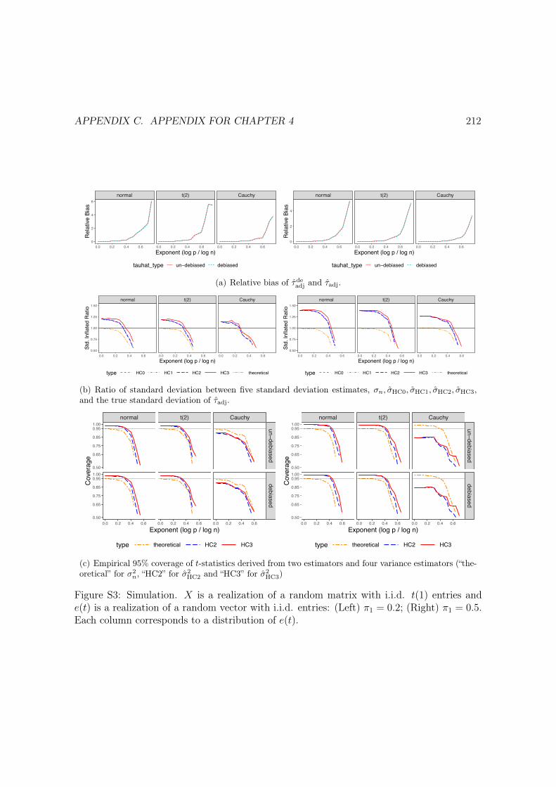
APPENDIX C. APPENDIX FOR CHAPTER 4 212
normal t(2) Cauchy
0.0 0.2 0.4 0.6 0.0 0.2 0.4 0.6 0.0 0.2 0.4 0.60
2
4
6
Exponent (log p / log n)
Rel
ative
Bia
s
tauhat_type un−debiased debiased
normal t(2) Cauchy
0.0 0.2 0.4 0.6 0.0 0.2 0.4 0.6 0.0 0.2 0.4 0.60
2
4
Exponent (log p / log n)
Rel
ative
Bia
s
tauhat_type un−debiased debiased
(a) Relative bias of ⌧deadj and ⌧adj.
normal t(2) Cauchy
0.0 0.2 0.4 0.6 0.0 0.2 0.4 0.6 0.0 0.2 0.4 0.60.50
0.75
1.00
1.25
1.50
Exponent (log p / log n)
Std.
Infla
ted
Rat
io
type HC0 HC1 HC2 HC3 theoretical
normal t(2) Cauchy
0.0 0.2 0.4 0.6 0.0 0.2 0.4 0.6 0.0 0.2 0.4 0.60.50
0.75
1.00
1.25
1.50
Exponent (log p / log n)
Std.
Infla
ted
Rat
io
type HC0 HC1 HC2 HC3 theoretical
(b) Ratio of standard deviation between five standard deviation estimates, �n, �HC0, �HC1, �HC2, �HC3,
and the true standard deviation of ⌧adj.
normal t(2) Cauchy
un−debiaseddebiased
0.0 0.2 0.4 0.6 0.0 0.2 0.4 0.6 0.0 0.2 0.4 0.6
0.50
0.65
0.75
0.85
0.951.00
0.50
0.65
0.75
0.85
0.951.00
Exponent (log p / log n)
Cov
erag
e
type theoretical HC2 HC3
normal t(2) Cauchy
un−debiaseddebiased
0.0 0.2 0.4 0.6 0.0 0.2 0.4 0.6 0.0 0.2 0.4 0.6
0.50
0.65
0.75
0.85
0.951.00
0.50
0.65
0.75
0.85
0.951.00
Exponent (log p / log n)
Cov
erag
e
type theoretical HC2 HC3
(c) Empirical 95% coverage of t-statistics derived from two estimators and four variance estimators (“the-
oretical” for �2n, “HC2” for �2
HC2 and “HC3” for �2HC3)
Figure S3: Simulation. X is a realization of a random matrix with i.i.d. t(1) entries ande(t) is a realization of a random vector with i.i.d. entries: (Left) ⇡1 = 0.2; (Right) ⇡1 = 0.5.Each column corresponds to a distribution of e(t).

APPENDIX C. APPENDIX FOR CHAPTER 4 213
0
5
10
15
0.0 0.2 0.4 0.6
Exponent (log p / log n)
Rel
ative
Bia
s
tauhat_type un−debiased debiased
0
5
10
15
0.0 0.2 0.4 0.6
Exponent (log p / log n)
Rel
ative
Bia
s
tauhat_type un−debiased debiased
(a) Relative bias of ⌧deadj and ⌧adj.
HC2 HC3
0.0 0.2 0.4 0.6 0.0 0.2 0.4 0.60.00
0.25
0.50
0.650.750.850.951.00
Exponent (log p / log n)
Cov
erag
e
tauhat_type un−debiased debiased
HC2 HC3
0.0 0.2 0.4 0.6 0.0 0.2 0.4 0.60.00
0.25
0.50
0.650.750.850.951.00
Exponent (log p / log n)
Cov
erag
e
tauhat_type un−debiased debiased
(b) Empirical 95% coverage of t-statistics derived from two estimators and two variance estimators (“HC2”
for �2HC2 and “HC3” for �2
HC3)
Figure S4: Simulation. X is a realization of a random matrix with i.i.d. t(1) entries and e(t)is defined in (4.27): (Left) ⇡1 = 0.2; (Right) ⇡1 = 0.5.

APPENDIX C. APPENDIX FOR CHAPTER 4 214
normal t(2) Cauchy
0 10 20 30 40 50 0 10 20 30 40 50 0 10 20 30 40 500.0
0.5
1.0
1.5
Number of covariates
Rel
ative
Bia
s
tauhat_type un−debiased debiased
(a) Relative bias of ⌧deadj and ⌧adj.
normal t(2) Cauchy
0 10 20 30 40 50 0 10 20 30 40 50 0 10 20 30 40 500.00
0.25
0.50
0.75
1.00
1.25
Number of covariates
Std.
Infla
ted
Rat
io
type HC0 HC1 HC2 HC3 theoretical
(b) Ratio of standard deviation between five standard de-
viation estimates, �n, �HC0, �HC1, �HC2, �HC3, and the true
standard deviation of ⌧adj.
normal t(2) Cauchy
un−debiaseddebiased
0 10 20 30 40 50 0 10 20 30 40 50 0 10 20 30 40 50
0.50
0.65
0.75
0.85
0.951.00
0.50
0.65
0.75
0.85
0.951.00
Number of covariates
Cov
erag
e
type theoretical HC2 HC3
(c) Empirical 95% coverage of t-statistics derived from two
estimators and four variance estimators (“theoretical” for �2n,
“HC2” for �2HC2 and “HC3” for �2
HC3)
Figure S5: Simulation on Lalonde dataset. e(t) is a realization of a random vector with i.i.d.entries. Each column corresponds to a distribution of e(t).

APPENDIX C. APPENDIX FOR CHAPTER 4 215
0
1
2
3
0 10 20 30 40 50
Number of covariates
Rel
ative
Bia
s
tauhat_type un−debiased debiased
(a) Relative bias of ⌧deadj and ⌧adj.
HC2 HC3
0 10 20 30 40 50 0 10 20 30 40 50
0.50
0.65
0.75
0.85
0.951.00
Number of covariates
Cov
erag
e
tauhat_type un−debiased debiased
(b) Empirical 95% coverage of t-statistics derived from two esti-
mators and two variance estimators (“HC2” for �2HC2 and “HC3”
for �2HC3)
Figure S6: Simulation on Lalonde dataset. e(t) is defined in (4.27).

APPENDIX C. APPENDIX FOR CHAPTER 4 216
normal t(2) Cauchy
0 10 20 30 40 50 0 10 20 30 40 50 0 10 20 30 40 50
0.025
0.050
0.075
Number of covariates
Rel
ative
Bia
s
tauhat_type un−debiased debiased
(a) Relative bias of ⌧deadj and ⌧adj.
normal t(2) Cauchy
0 10 20 30 40 50 0 10 20 30 40 50 0 10 20 30 40 50
0.50
0.75
1.00
Number of covariates
Std.
Infla
ted
Rat
io
type HC0 HC1 HC2 HC3 theoretical
(b) Ratio of standard deviation between five standard de-
viation estimates, �n, �HC0, �HC1, �HC2, �HC3, and the true
standard deviation of ⌧adj.
normal t(2) Cauchy
un−debiaseddebiased
0 10 20 30 40 50 0 10 20 30 40 50 0 10 20 30 40 50
0.50
0.65
0.75
0.85
0.951.00
0.50
0.65
0.75
0.85
0.951.00
Number of covariates
Cov
erag
e
type theoretical HC2 HC3
(c) Empirical 95% coverage of t-statistics derived from two
estimators and four variance estimators (“theoretical” for �2n,
“HC2” for �2HC2 and “HC3” for �2
HC3).
Figure S7: Simulation on STAR dataset. e(t) is a realization of a random vector with i.i.d.entries. Each column corresponds to a distribution of e(t).

APPENDIX C. APPENDIX FOR CHAPTER 4 217
0.0
0.5
1.0
1.5
0 10 20 30 40 50
Number of covariates
Rel
ative
Bia
s
tauhat_type un−debiased debiased
(a) Relative bias of ⌧deadj and ⌧adj.
HC2 HC3
0 10 20 30 40 50 0 10 20 30 40 50
0.50
0.65
0.75
0.85
0.95
Number of covariates
Cov
erag
e
tauhat_type un−debiased debiased
(b) Empirical 95% coverage of t-statistics derived from two esti-
mators and two variance estimators (“HC2” for �2HC2 and “HC3”
for �2HC3).
Figure S8: Simulation on STAR dataset. e(t) is defined in (4.27).