Purdue UniversityPurdue e-Pubs
ECE Technical Reports Electrical and Computer Engineering
12-1-1993
MODELING AND ANALYSIS OFDISTRIBUTION LOAD CURRENTSPRODUCED BY AN AD JUSTABLE SPEEDDRIVE HEAT PUMPStephen Paul HoffmanPurdue University School of Electrical Engineering
Follow this and additional works at: http://docs.lib.purdue.edu/ecetr
This document has been made available through Purdue e-Pubs, a service of the Purdue University Libraries. Please contact [email protected] foradditional information.
Hoffman, Stephen Paul, "MODELING AND ANALYSIS OF DISTRIBUTION LOAD CURRENTS PRODUCED BY AN ADJUSTABLE SPEED DRIVE HEAT PUMP" (1993). ECE Technical Reports. Paper 258.http://docs.lib.purdue.edu/ecetr/258
MODELING AND ANALYSIS OF
DISTRIBUTION LOAD CURRENTS
PRODUCED BY AN ADJUSTABLE
SPEED DRIVE HEAT PUMP
TR-EE 93-51 DECEMBER 1993
MODELING AND ANALYSIS OF DISTRIBUTION
LOAD CURRENTS PRODUCED BY AN
AD JUSTABLE SPEED DRIVE HEAT PUMP
Stephen Paul Hoffman
Purdue Electric Power Center
School of Electrical Engineering
Purdue University
1285 Electrical Engineering Building
West Lafayette, IN 47907-1285
December 1993

TABLE OF CONTENTS
Page
LIST OF TABLES .............................................................................................. v
LIST OF FIGURES ............................................................................................. vi
NOMENCLATURE.. ... ... ... ... ........ .... ........... .. .............. ... ........................ ...... ......... x
ABSTRACT ........................................................................................................ xx
CHAPTER 1. INTRODUCTION ........................................................................... 1
. . 1.1 Motivation ..................................................................................... 1 1.2 Scope .............................................................................................. 3 1.3 Adjustable speed drives ................................................................... 4 1.4 Transformers .................................................................................... 8
1.4.1 Distribution transformers ..................................................... 8 1.4.2 Transformer losses ............................................... ................ 9 1.4.3 Transformer thermal damage ..... ................. ..................... . 9 1.4.4 American National Standard
Institute document C57.110 ................................................. 10
CHAPTER 2. ADJUSTABLE SPEED DRIVE HEAT PUMPS ............................ 13
2.1 Refrigeration cycle ............. . .. ....... ... ... ... . . . . ................... . . . . 13 2.2 Adjustable speed drive heat pumps .................................. ................ 18

Page
CHAPTER 3 . MODELING OF THE ASD HEAT PUMP ..................................... 22
3.1 Introduction ..................................................................................... 22 3.2 Modeling of the electric motor ........................................................ 23 3.3 Modeling of the adjustable speed drive ........................................... 34
3.3.1 Introduction ......................................................................... 34 3.3.2 VSI-ASD inverter ............................................................... 36 3.3.3 VSI-ASD rectifier operation ................................................ 40
3.4 Modeling of the distribution transformer ........................................... 42 3.5 Modeling of the compressor shaft load ............................................ 44 3.6 ACSL program explanation and listing ............................................ 45
CHAPTER 4 . SIMULATION RESULTS AND ANALYSIS ................................ 54
4.1 Introduction .................................................................................... 54 4.2 Simulation results ............................................................................ 55 4.3 Field measurement cases .................................................................. 75 4.4 Transformer derating calculations .................................................... 80
.................................... 4.4.1 ANSI C57.110 example calculation 80 .................................. 4.4.2 Transformer derating of actual system 81
4.4.3 Transformer derating for simulation results .......................... 83 4.5 IEEE Standard 519-1992 ................................................................ 86
CHAPTER 5 . CONCLUSIONS AND RECOMMENDATIONS ........................... 89
5.1 Conclusions ...................................................................................... 89 5.2 Recommendations ........................................................................... 90
.................................................................................................. BIBLIOGRAPHY 92

LIST OF TABLES
Table Page
ASD figure description, no load case ......................................................... 56
Simulated motor load torque cases ............................................................. 58
Figure descriptions of field measurements ................................................... 75
.............................................. ANSI C57.110 transformer derating example 8 1
Transformer active power loss estimates ............................................................. for the actual measurements 82
Transformer active power loss estimates for the simulation results, load 3 ...................................................... 84
Transformer primary and secondary current total harmonic distortion and derating for the five load cases .................................................................... 85
Transformer derating for the five load cases, transformer at rated load, one-half
......................................................... ASD and full ASD load cases 86
IEEE Standard 5 19- 1992 Current distortion limits for general destribution
................................ systems (120 volts through 69,000 volts) [11] 87
THD and transformer derating results for simulated and measured waveforms ................................................ 90

LIST OF FIGURES
Figure Page
1.1 Drive system showing controller. converter. ......................................................................... motor. and process 4
1.2 Simplified diagram of adjustable speed drive ............................................... 5
1.3 Voltage source inverter adjustable speed drive ............................................ 7
.......................................................................... 1.4 Transformer configuration 8
2.1 Refrigeration cycle block diagram ............................................................... 14
............................................. 2.2 Reversible refrigeration cycle in cooling mode 15
............................................. 2.3 Reversible refrigeration cycle in heating mode 16
............................................................... 2.4 Block diagram of ASD heat pump 21
..................... 3.1 Side view of motor with stator winding ................................... 24
3.2 Winding turns density versus Or ................................................................. 25
3.3 Cross-sectional view of induction motor showing the locations of the rotor and stator windings ...................................... 25
3.4 Equivalent circuit of induction machine ....................................................... 26
3.5 Figure showing relationship between (abc) and (qdo) variables ............................................................................... 31
3.6 Voltage source inverter adjustable speed drive ............................................ 34
3.7 Six step voltage waveform ........................................................................... 35
3.8 Voltage source inverter. 3-phase ................................................................. 36 . .
3.9 Inverter switching strategy .......................................................................... 38
vii
Figure Page
Six step inverter waveform .......................................................................... 39
Single phase rectifier with LC filter ............................................................. 41
Transformer equivalent circuit diagram ....................................................... 44
.............................. Transformer and drive with ACSL program parameters 53
Transformer primary voltage versus time .................................................... 59
Transformer input current versus time ....................................................... 59
Transformer instantaneous power versus time ............................................. 59
Phase a inverter six step output voltage versus time .................................... 60
Phase b inverter six step output voltage versus time .................................... 60
Phase c inverter six step output voltage versus time .................................... 60
Induction motor speed versus time .............................................................. 61
Induction motor electrical torque versus time .............................................. 61
Inverter input voltage Vinv versus time ....................................................... 61
Frequency spectrum of inverter output voltage Vas ..................................... 62
Frequency spectrum of transformer secondary current ................................ 62
Frequency spectrum of phase a motor stator current ................................. 62
Induction motor speed versus time ............................................................. 63
Induction motor electrical torque versus time .............................................. 63
Applied load torque versus time .................................................................. 63
Transformer secondary current versus time .................................................. 64
Transformer primary instantaneous power versus time ................................. 64
Inverter input voltage versus time ............................................................... 64
Load 1. Transformer primary current versus time ........................................ 65
Load 1. Transformer secondary current versus time ..................................... 65
Figure Page
...................................... Load 1. Transformer primary instantaneous power 65
Load 1. Frequency spectrum of transformer secondary current expressed as a percentage of the fundamental ........................................................ 66
Load 1. Frequency spectrum of transformer primary current expressed as a percentage of the fundamental ........................................................ 66
Load 2. Transformer primary current versus time ........................................ 67
Load 2. Transformer secondary current versus time .................................... 67
...................................... Load 2. Transformer primary instantaneous power 67
Load 1. Frequency spectrum of transformer secondary current expressed as a percentage of the fundamental ........................................................ 68
Load 1. Frequency specbum of transformer primary current expressed as a percentage of the fundamental ......................................................... 68
Load 3. Transformer primary current versus time ........................................ 69
Load 3. Transformer secondary current versus time .................................... 69
Load 3. Transformer primary instantaneous power ................................... 69
Load 3. Frequency spectrum of transformer secondary current expressed as a
.......................................................... percentage of the fundamental 70
Load 3. Frequency spectrum of transformer primary current expressed as a
......................................................... percentage of the fundamental 70
Load 4. Transformer primary current versus time ........................................ 71
Load 4. Transformer secondary current versus time .................................... 7 1
Load 4. Transformer primary instantaneous power ...................................... 71

Figure Page
Load 4. Frequency spectrum of transformer secondary current expressed as a
......................................................... percentage of the fundamental 72
Load 4. Frequency spectrum of transformer primary current expressed as a
......................................................... percentage of the fundamental 72
Load 5. Transformer primary current versus time ........................................ 73
Load 5. Transformer secondary current versus time .................................... 73
Load 5. Transformer primary instantaneous power ...................................... 73
Load 5. Frequency spectrum of transformer secondary current expressed as a percentage of the fundamental ......................................................... 74
Load 5. Frequency spectrum of transformer primary current expressed as a percentage of the fundamental ......................................................... 74
Phase a current and voltage snapshot. heat pump off ................................... 76
Phase a instantaneous power. heat pump off ............................................... 76
Phase a voltage amplitude spectrum. heat pump off ..................................... 77
Phase a current amplitude spectrum. heat pump off ..................................... 77
Phase a current and voltage snapshot. heat pump on ................................... 78
Phase a instantaneous power. heat pump on ................................ , ................ 78
Phase a voltage amplitude spectrum. heat pump on ..................................... 79
Phase a current amplitude spectrum. heat pump on ..................................... 79

NOMENCLATURE
ac alternating current
ACSL Advanced Continuous Simulation Language
alpha rectifier firing delay angle variable
ANSI American National Standards Institute
ANSI C57.110 Recommended Practice for Establishing Transfornier Capability when Supplying Nonsinusoidal Load Currents
ar subscript to denote the a rotor phase winding
as subscript to denote the a stator phase winding
ASD adjustable speed drive
br subscript to denote the b rotor phase winding
bs subscript to denote the b stator phase winding
c f capacitance of parallel capacitor
cint ACSL variable to determine data logging rate
COP coefficient of performance
cr subscript to denote the c rotor phase winding
cs subscript to denote the c stator phase winding
dc direct current
DSM demand side management
EER energy efficiency ratio
fabcr 3 by 1 column vector of a, b, and c rotor parameters f abcr 3 by 1 column vector of a, b, and c rotor parameters
referred to the stator windings
fabcs
FFT
fh
Fme
f qdor
gtzero
h
HP
HVAC
Iabcr
f abcr
Iabcs
ialg
iar
ias
ibr
ibs
icr
ics
i'dr
idrs
ids
idss
3 by 1 column vector of a, b, and c stator parameters
fast Fourier transform
harmonic current distribution factor for harmonic h
frequency of the inverter ac output waveform
frequency of fundamental component
3 by 1 column vector of a, b, and c rotor parameters referred to the stator windings
logical variable used to determine rectifier state
harmonic order
heat pump
heating, ventilation, and air conditioning
3 by 1 column vector of a, b, and , rotor phase currents
3 by 1 column vector of a, b, and c rotor phase currents referred to the stator windings
3 by 1 column vector of a, b, and , stator phase currents
ACSL constant to determine integration algorithm
current into phase a or induction motor rotor winding
current into phase a of induction motor stator winding
current into phase b of induction motor rotor winding
current into phase b of induction motor stator winding
current into phase c of induction motor rotor winding
current into phase c of induction motor stator winding
d axis rotor current referred to the stator windings
current through d rotor winding
current through d stator winding
current through d stator winding
iqdos
i'qr
idrs
iqs
iqss
current into the inverter
current through the inductor Lf
current through inductor Lf initial condition
rms load current
3 by 1 column vector of q, d, and 0 rotor currents referred to the stator windings
3 by 1 column vector of q, d, and 0 stator currents
q axis rotor current referred to the stator windings
current through d rotor winding
current through q stator winding
current through q stator winding
current drawn by the rectifier
induction motor stator winding current
0 axis rotor current referred to the stator windings
current through 0 stator winding
current into the transformer primary winding
current into the transformer secondary winding
transformer secondary current referred to the primary
transformer secondary current referred to the primary
induction motor rotor inertia
kiloamps
3 by 3 rotor arbitrary reference frame transformation
3 by 3 stator arbitrary reference frame transformation
kilovolts
kilovolt-amps
inductance of series smoothing inductor

Ls
Lsr
L'sr
Lsrrn
maxt
mint
Nr
N I
N2
M
induction motor rotor leakage inductance
induction motor rotor leakage inductance referred to the stator windings
induction motor stator leakage inductance
transformer secondary leakage inductance referred to the primary
induction motor rotor mutual inductance
induction motor stator mutual inductance
3 by 3 matrix of rotor leakage and mutual inductances
3 by 3 matrix of rotor leakage and mutual inductances referred to the stator windings
3 by 3 matrix of stator leakage and mutual inductances
maximum mutual inductance between stator and rotor
maximum mutual inductance between stator and rotor referred to the stator windings
mutual inductance between stator and rotor windings
ACSL maximum integration step size constant
ACSL minimum integration step size constant
number of turns in rotor phase winding
number of t w s in transfo_mcr primary winding
number of turns in transformer secondary winding
1.5 times the stator mutual inductance
number of turns in stator phase winding
derivative with respect to time operator
number of poles in induction motor
time derivative of the inductor current
time derivative of the inductor current when switch is on
time derivative of the inductor current when Vrec < 0

pilonplus
PEC-R(P~)
PLI,-R(P~)
PramP
PramPP
pSidrs
pSidss
pS iqrs
pSiqss
rampic
ramppic
Rload
rms
Ron
r r
time derivative of the inductor current when Vrec > 0
per unit winding eddy current loss for rated conditions
per unit load loss density under rated conditions
time derivative of ramp to determine inverter switching
time derivative of ramp to determine rectifier switching
time derivative of rotor d axis flux linkage per second
time derivative of stator d axis flux linkage per second
time derivative of rotor q axis flux linkage per second
time derivative of stator q axis flux linkage per second
time derivative of the transformer primary flux linkage per second
time derivative of the transformer secondary flux linkage ]per second
time derivative of the voltage across the capacitor Cf
time derivative of rotor angular velocity
inverter switching ramp function initial condition
rectifier switching ramp function initial condition
resistance of load across transformer secondary
root mean square
logical variable used to determine rectifier state
induction motor rotor phase winding resistance
induction motor rotor phase winding resistance referred to the stator windings
3 by 3 diagonal matrix with diagonal entries equal to rr
3 by 3 diagonal matrix with diagonal entries equal to rtr
induction motor stator phase winding resistance
3 by 3 diagonal matrix with diagonal entries equal to rs
resistance of transformer primary winding

SCR
Sidrs
Sidrsic
Sidss
Sidssic
Sirn
sirnd
sirnq
Siqrs
Siqrsic
Siqss
Siqssic
Sil
Silic
t
Tconstant
transformer secondary resistance referred to the primary
transformer secondary resistance referred to the primary
logical variable used to determine inverter state
logical variable used to determine inverter state
logical variable used to determine inverter state
silicon controlled rectifier
induction motor d axis rotor flux linkage per second
induction motor d axis rotor flux linkage per second initial condition
induction motor d axis stator flux linkage per second
induction motor d axis stator flux linkage per second initkl condition
transformer mutual flux linkage per second
induction motor flux linkage per second parameter
induction motor flux linkage per second parameter
induction motor q axis rotor flux linkage per second
induction motor q axis rotor flux linkage per second initia:l condition
induction motor q axis stator flux linkage per second
induction motor q axis stator flux linkage per second initial condition
transformer primary flux linkage per second
transformer primary flux linkage per second initial condition
transformer secondary flux linkage per second referred to the primary
transpose
transformer secondary flux linkage per second initial condition referred to the primary winding
time in ACSL simulation
constant component of compressor load torque

I
xvi
TDD
THD
Te
Tm
tstop
T1
Tvar
twopi
v
Vabcr
V'abcr
Vabcs
Vag
V ~ P
var
Vas
vbg
V ~ P
vbr
vbs
vcg
VCP
Vcr
vcs
V'dr
total harmonic distortion
total harmonic distortion
electrical torque produced by the motor
inverter output waveform period
ACSL variable to determine simulation stop time
load torque applied to the induction motor
time-varying component in compressor load torque
constant equal to two times pi
volts
3 by 1 column vector of a, b, and c rotor phase voltages
3 by 1 column vector of a, b, and c rotor phase voltages referred to the stator windings
3 by 1 column vector of a, b, and c stator phase voltages
voltage from node a to ground in Figure (3.8)
voltage from nodes a to p in Figure (3.8)
voltage across induction motor phase a rotor winding
voltage across induction motor phase a stator winding
voltage from node b to ground in Figure (3.8)
voltage from nodes b to p in Figure (3.8)
voltage across induction motor phase b rotor winding
voltage across induction motor phase b stator winding
voltage from node c to ground in Figure (3.8)
voltage from nodes c to p in Figure (3.8)
voltage across induction motor phase c rotor winding
voltage across induction motor phase c stator winding
d axis rotor voltage referred to the stator windings

I
xvii
vdrs
Vds
vdss
vinv
Vinvic
Vm
vmag
Vng
V ~ P
Vqdos
V'qr
vqrs
vqs
vqs s
Vrec
VSI
V'0r
vos
v 1
v 2
V'2
v2pr
wb
voltage across d rotor winding
voltage across d stator winding
voltage across d stator winding
voltage applied to the inverter and across capacitor Cf
voltage applied to the inverter initial condition
transformer reference voltage
magnitude of the sinusoidal transformer primary voltage
voltage from node n to ground in Figure (3.8)
voltage from nodes n to p in Figure (3.8)
3 by 1 column vector of q, d, and 0 rotor voltages referred to the stator windings
3 by 1 column vector of q, d, and 0 stator voltages
q axis rotor voltage referred to the stator winding
voltage across d rotor winding
voltage across q stator winding
voltage across q stator winding
voltage applied to the single phase rectifier
voltage source inverter
0 axis rotor voltage referred to the rotor windings
voltage across 0 stator winding
voltage applied to the transformer primary winding
voltage applied to the transformer secondary winding
transformer secondary voltage referred to the primary
transformer secondary voltage referred to the primary
base frequency in radians per second
source electrical frequency in radians per second
wric
wsl
Xad
xcapm
Xaq
Xlr
Xls
xll
induction motor rotor angular velocity
induction motor rotor base frequency
induction motor rotor angular velocity initial condition
induction motor slip frequency in radians per second
induction motor d axis reactance constant
transformer reactance constant
induction motor q axis reactance constant
induction motor rotor leakage reactance
induction motor stator leakage reactance
transformer primary leakage reactance
transformer secondary leakage reactance referred to the primary winding
induction motor mutual reactance
transformer mutual reactance
rotor arbitrary reference frame transformation angle
stator arbitrary reference frame transformation angle
induction motor rotor angle
3 by 1 column vector of a, b, and c rotor flux linkages
3 by 1 column vector of a, b, and c rotor flux linkages referred to the stator windings
3 by 1 column vector of a, b, and c stator flux linkages
3 by 1 column vector with entries kdr, -kqr, and 0
3 by 1 column vector with entries a s , -hqs, and 0
flux linking d rotor winding referred to the stator winding
flux linking d stator winding

3 by 1 column vector of q, d, and 0 rotor flux linkages referred to stator windings
3 by 1 column vector of q, d, and 0 stator flux linkages
flux linking q rotor winding referred to the stator winding
flux linking q axis stator winding
flux linking 0 rotor winding referred to the stator winding
flux linking 0 stator winding
arbitrary reference frame velocity
induction machine rotor velocity
velocity of compressor shaft
transformer mutual flux linkage per second

ABSTRACT
A number of demand side management techniques have been proposed for the
efficient use of electric power in the commercial and residential sector:;. The adjustable
speed.drive heat pump is a technology which has the prospect of decreasing power
demands for space heating. This design has the advantage over conventional designs of
higher efficiency and, potentially, reduction of peak power demand. Its main disadvantage
is higher cost. Further, it has the disadvantage that it produces a load current with a
substantial harmonic content. This load current waveform is injected into the distribution
system and causes extra losses in the distribution transformer. These high efficiency heat
pumps are being promoted by some utility rebate programs to encourage residential
customers to install the high efficiency devices. This thesis presents an introduction to
adjustable speed drives as they are applied to the refrigeration cycle. The impact of these
devices on distribution transformers and the significant transformer derating is discussed.
In addition, an Advanced Continuous Simulation Language, (ACSL), simulation is
presented that models the induction motor, six step adjustable speed drive, and
distribution transformer. The results of this simulation are presented1 to show typical
system waveforms, such as the load current and its frequency spectrum. These waveforms
are compared to results obtained from an actual installation. In addition, the ANSI

Standard C57.110 is used to assess the transformer derating. The main contribution of the
thesis is the presentation of a detailed method for the analysis of adjustable speed drive
heat pump loads. General conclusions are drawn concerning the appliciability of the high
efficiency, adjustable speed drive heat pump including the added losses in the distribution
system.

CHAPTER 1
INTRODUCTION
1.1 Motivation
In recent years, due to the high cost of adding power generation, transmission, and
distribution capacity, many electric utility companies have instituted various programs
with the intent of forestalling system expansion. Also, in many jurisdictions, regulatory
agencies critically examine applications for system expansion because they are under
pressure from consumer groups to minimize all costs which are placed in the rate base,
including those costs for system expansion. Among these efforts are programs to reduce
the peak demand. One class of such programs are termed demand side management
(DSM) programs. Demand side management programs include such efforts as control of
air conditioners and electric water heaters during peak periods. Other commonly used
techniques for reducing the electrical peak demand are making use of interconnections
with neighbors, applications of cogeneration, conservation, and taking advantage of the
modem technologies which increase the efficiency of loads. These programs are designed
to reduce both the peak demand and the total electric energy consumedl. If the electrical
demand, or its growth, is reduced the presently installed generation, transmission, and
distribution capacity may be sufficient to supply the load for a longer bime. In this way,
electric utility companies can get the maximum use from their installed facilities.
The three most frequently used programs for peak demand reduction and total
energy use reduction are demand side management, conservation, and increased efficiency.

Demand side management refers to direct control of loads by the electric utility company.
Using direct control, the peak demand can be reduced by shifting loads in time from on-
peak to off-peak hours. Conservation programs refer to voluntary reduction of the load
during both on-peak and off-peak hours by the elimination of electric energy use by some
non-critical loads that would have otherwise been required. Conservation includes such
measures as a decreased household heating temperature, a higher household cooling set-
point temperature, reduced lighting load, and a lower water heater ternperature setting.
The third demand reduction program, improvement of load efficiencies, may be the most
important method to achieve a reduction in the load. Unlike the first two methods,
improving load efficiencies does not entail sacrifice or change of life style by individual
residential or commercial consumers. Improvements of load efficiencies have been
implemented or are being studied in diverse applications such as electric clothes dryers (a
microwave clothes dryer has been proposed), high efficiency motors, electric ballasts for
fluorescent lighting, novel lighting designs to replace the conventional incandescent lamp,
high efficiency refrigerators, water heaters, dishwashers, and heat pumps. Demand side
management, conservation, and improved efficiency programs for manly utilities include
rebates and other incentives.
The energy required to heat or cool a residential and cornrnercial building
represents a significant percentage of the total electric energy consunled in the United
States. Within a given region of the country, the heating and cooling load depends largely
on weather related factors. Most utilities in the United States, except for those in the far
North, experience their peak load during the summer months due to the extra energy
required to serve air conditioning loads. An improvement in the efficiency of air
conditioners would reduce the peak load served by these utilities. Al.though the utility
may lose revenue due to increased efficiency, a reduction in peak load is an advantage for
a utility because generation and transmission installation requirements are determined from
the peak load. If a utility can limit its peak load the need for new generating units can be
postponed. In this manner, a company whose business is to sell electric power can justify
encouraging consumers to install energy-efficient air conditioning units. Utilities are also
under regulatory pressure to promote energy conservation, and it is a prudent practice to
conserve energy and resources whenever possible.
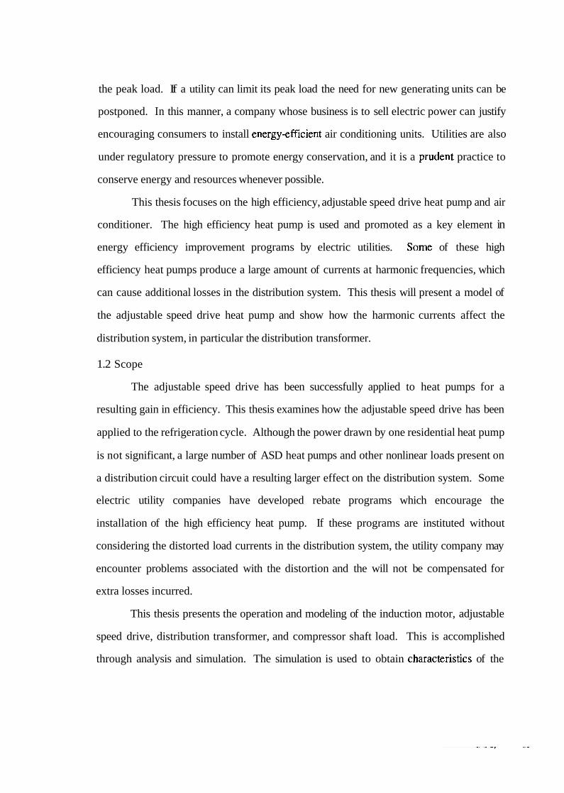
This thesis focuses on the high efficiency, adjustable speed drive heat pump and air
conditioner. The high efficiency heat pump is used and promoted as a key element in
energy efficiency improvement programs by electric utilities. Sorrie of these high
efficiency heat pumps produce a large amount of currents at harmonic frequencies, which
can cause additional losses in the distribution system. This thesis will present a model of
the adjustable speed drive heat pump and show how the harmonic currents affect the
distribution system, in particular the distribution transformer.
1.2 Scope
The adjustable speed drive has been successfully applied to heat pumps for a
resulting gain in efficiency. This thesis examines how the adjustable speed drive has been
applied to the refrigeration cycle. Although the power drawn by one residential heat pump
is not significant, a large number of ASD heat pumps and other nonlinear loads present on
a distribution circuit could have a resulting larger effect on the distribution system. Some
electric utility companies have developed rebate programs which encourage the
installation of the high efficiency heat pump. If these programs are instituted without
considering the distorted load currents in the distribution system, the utility company may
encounter problems associated with the distortion and the will not be compensated for
extra losses incurred.
This thesis presents the operation and modeling of the induction motor, adjustable
speed drive, distribution transformer, and compressor shaft load. This is accomplished
through analysis and simulation. The simulation is used to obtain cha.racteristics of the

system behavior during various operating conditions. The fast Fourier transform, FFT, is
also used to obtain the frequency spectrum of selected waveforms. The simulation results
are compared to waveforms obtained from an operating adjustable speed drive heat pump.
Calculations are presented which show the transformer derating for typical operating
conditions with a nonlinear load.
1.3 Adjustable speed drives
An adjustable speed drive (ASD) is a solid state device which controls the energy
flow to a rotating machine for the purpose of controlling its operation. A motor drive
consists of the controller, power electronic converter, electric motor, a~nd possibly speed
and position sensors. A block diagram of a power electronic drive system is shown in
Figure (1.1). The purpose of the drive is to directly control the voltage, current, and
frequency applied to the electric motor so that the motor outputs, such as speed and
torque, are as desired for a particular application. Power electronic drives are typically
connected to an alternating current supply and are used to control synchronous, direct
current, induction, and stepper motors. Motor drives are in operation that can supply and
control motors ranging in size from several watts up to several thousand horsepower [12].
input Power I
- Process Control
Power
I-
Figure 1.1 Drive sys tem showing controller, converter, motor, and process
Controller Converter
- Electronic m t o r m Process -
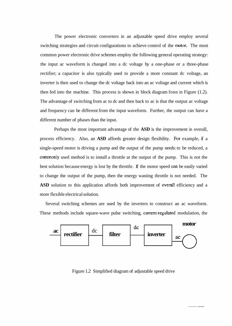
The power electronic converters in an adjustable speed drive employ several
switching strategies and circuit configurations to achieve control of the ]motor. The most
common power electronic drive schemes employ the following general operating strategy:
the input ac waveform is changed into a dc voltage by a one-phase or a three-phase
rectifier; a capacitor is also typically used to provide a more constant dc voltage, an
inverter is then used to change the dc voltage back into an ac voltage and current which is
then fed into the machine. This process is shown in block diagram fonn in Figure (1.2).
The advantage of switching from ac to dc and then back to ac is that the output ac voltage
and frequency can be different from the input waveform. Further, the output can have a
different number of phases than the input.
Perhaps the most important advantage of the ASD is the improvement in overall,
process efficiency. Also, an ASD affords greater design flexibility. ]?or example, if a
single-speed motor is driving a pump and the output of the pump needs: to be reduced, a
conlmonly used method is to install a throttle at the output of the pump. This is not the
best solution because energy is lost by the throttle. If the motor speed can be easily varied
to change the output of the pump, then the energy wasting throttle is not needed. The
ASD solution to this application affords both improvement of overall. efficiency and a
more flexible electrical solution.
Several switching schemes are used by the inverters to construct an ac waveform.
These methods include square-wave pulse switching, current-regulated modulation, the
Figure 1.2 Simplified diagram of adjustable speed drive
motor ac
rectifier dc
filter inverter dc
-Q

voltage-cancellation technique, and pulse-width modulation [7]. This last method has the
advantage that the output frequency and voltage magnitude is con,trollable and the
harmonics in the output waveform are lower than with other methods. :More information
on other novel and proposed drive topologies, such as the matrix converter, the current
link converter, the resonant link converter, can be found in [12].
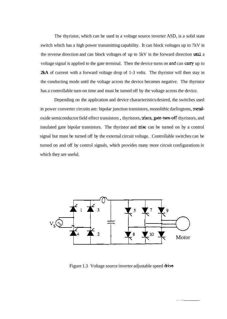
The voltage source inverter employs one of the simplest switching strategies and is
favored because of its low switching frequency requirements. This adjustable speed drive
design is also rugged, but has the disadvantages of a poor power factor at low speeds and
low speed pulsations. The circuit diagram for the voltage source inverter is shown in
Figure (1.3). The single phase, usually 60 hertz supply is connected to a rectifier. The
rectifier can be constructed with diodes to give an uncontrolled dc output voltage. For
induction motor drives the rectifier is usually constructed with thyristor;^. Thyristors can
be controlled to yield a variable output voltage. The series inductor and parallel capacitor
between the rectifier and inverter reduces the pulsations in the dc voltage which supplies
the inverter. The inverter uses thyristors or some other controllable switch to produce a
thre,e phase, six-step waveform which is fed into the machine. Referring to Figure (1.3),
the inverter is controlled such that a switch is turned on for 180 electrical degrees. The
resulting output of this switching pattern is a three phase, six step output voltage
waveform which is used to drive a machine. The intermediate dc voltage isolates the input
ac from the output ac, which is why the output can have a different number of phases,
voltage level, and frequency than the input waveform.
The thyristor, which can be used in a voltage source inverter ASD, is a solid state
switch which has a high power transmitting capability. It can block voltages up to 7kV in
the reverse direction and can block voltages of up to 5kV in the forward direction until a
voltage signal is applied to the gate terminal. Then the device turns on a:nd can cany up to
2kA of current with a forward voltage drop of 1-3 volts. The thyristor will then stay in
the conducting mode until the voltage across the device becomes negative. The thyristor
has a controllable turn-on time and must be turned off by the voltage across the device.
Depending on the application and device characteristics desired, the switches used
in power converter circuits are: bipolar junction transistors, monolithic darlingtons, metal-
oxide semiconductor field effect transistors , thyristors, macs, gate-turn-,off thyristors, and
insulated gate bipolar transistors. The thyristor and mac can be turned on by a control
signal but must be turned off by the external circuit voltage. Controllable switches can be
turned on and off by control signals, which provides many more circuit configurations in
which they are useful.
I C I , .
2 8 10 Motor
Figure 1.3 Voltage source inverter adjustable speed drive
1.4 Transformers
1.4.1 Distribution transformers
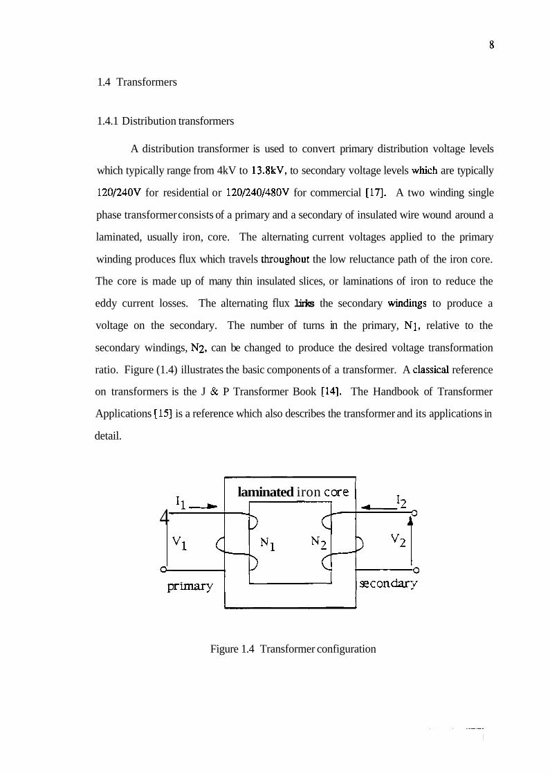
A distribution transformer is used to convert primary distribution voltage levels
which typically range from 4kV to 13.8kV, to secondary voltage levels which are typically
120/240V for residential or 120/240/480V for commercial [17]. A two winding single
phase transformer consists of a primary and a secondary of insulated wire wound around a
laminated, usually iron, core. The alternating current voltages applied to the primary
winding produces flux which travels throughout the low reluctance path of the iron core.
The core is made up of many thin insulated slices, or laminations of iron to reduce the
eddy current losses. The alternating flux links the secondary windings to produce a
voltage on the secondary. The number of turns in the primary, N1, relative to the
secondary windings, N2, can be changed to produce the desired voltage transformation
ratio. Figure (1.4) illustrates the basic components of a transformer. A lclassical reference
on transformers is the J & P Transformer Book [14]. The Handbook of Transformer
Applications [15] is a reference which also describes the transformer and its applications in
detail.
laminated iron core
4
Figure 1.4 Transformer configuration
1.4.2 Transformer losses
Any real device will consume energy during operation, and the transformer is no
exception. The losses in a transformer can be divided into the copper losses, stray losses,
and the no-load or the excitation loss. The wire windings of the transformer have a small
resistance. The current flowing through the windings will cause the I:'R copper losses.
The stray losses are made up of the eddy current losses in the windings and in the other
metal components of the transformer. This stray loss occurs because the leakage flux
induces a voltage in the metal of the transformer which causes circular, or eddy, currents
to flow. The metal has an electrical resistance so heat is produced by the eddy currents
which is lost energy. The eddy current losses are proportional to the square of the load
current multiplied by the square of the frequency [2].
1.4.3 Transformer thermal damage
The power lost in a transformer is converted to thermal energy. The thermal
energy raises the temperature of the transformer. Transformer losses must be limited so
that the internal temperature is not so high that damage to the transfor~mer would result.
Several of the methods used to cool a transformer are: oil bath ~urroun~ding the core and
windings, a heat exchanger, and cooling fans.
Transformer damage resulting from increased internal temperature can occur in
several ways. The highest temperature, often referred to as the hot spot, in the
transformer must be limited so that the device is not permanently physically damaged. The
operating lifetime of the transformer can also be reduced by high operating temperatures.
The conventional insulation between conductors turn-to-turn used in tra~lsformers consists
of lacquer and a paper or cloth material which contains cellulose. Lacquer is a complex
organic compound. Cellulose is a complex organic compound whose molecules are made
up of 1000 to 1400 glucose monomers, which are a combination of carbon, oxygen, and
hydrogen atoms [18]. Extreme heat will cause charring of the insulation. However, even
moderately high temperatures cause a breakdown in the individual monomers in the large
cellulose molecule. The thermal aging of cellulose insulation deteriorates its mechanical
properties, such as tensile strength, burst, and tear properties. Although cellulose is
adversely affected by water and oxygen, modern oil preservation system:< are employed to
minimize the water and oxygen content in a transformer. The transforn~er temperature is
determined by the operating conditions primarily the load level, power factor, and duration
of the load. Also, the temperature depends on the losses, which in part depend on the
level and the total harmonic distortion of the current. Thus thermal operating conditions
can reduce the useful operating lifetime of the transformer. Mechanical and dielectric
stresses more frequently determine the transformer life, although thermally induced
insulation deterioration can make a transformer more susceptible to mechanical or
dielectric stresses.
1.4.4 American National Standards Institute document (257.1 10
The American National Standards Institute, ANSI, jointly with the IEEE, has
estimated and quantified the reduction in transformer capacity when it is forced to carry
nonsinusoidal load currents. This work appears in ANSI C57.110, "Recommended
Practice for Establishing Transformer Capability when Supplying Nonsinusoidal Load
Currents." A distribution transformer is designed to operate with sinusoidal voltages and
currents at the fundamental frequency of 60 hertz. Loads such as incandescent lamps,
induction motors, resistive heating, and power factor correction capacitors do not
significantly distort the sinusoidal voltage and current waveforms. Since the voltage and
current waveforms are not distorted, the harmonic content in the current drawn by these
loads is low.
The number of power electronic loads served by the distribution system has
increased. The main power electronic load is the industrial rectifier. Other nonlinear loads
are: fluorescent lighting, lighting dimmers, electronic devices such as televisions and
computers, and drives for rotating machines. Power electronic drives use solid-state
switches which interrupt the current drawn by a load and reconnect it during any portion
of the cycle [13]. Although the operating characteristics of these drives can vary widely
depending on the design, the current drawn by these power electronic loads is often not
sinusoidal. In most cases the input current to a drive is a square wave or other non-
sinusoidal wave, which contains a significant percentage of harmonics. A harmonic
current is a sinusoidal wave with a frequency that is an integer multiple of the 60 hertz
fundamental frequency. The harmonic is one term of the Fourier series rlepresentation of a
periodic signal. Since the impedance of the power system source is lower than the
impedance of the power electronic load, a power electronic load appears to the
distribution line as a harmonic current source. The distribution transformer is forced to
carry these non-sinusoidal currents which are injected into the distribution system. The
higher frequency sinusoids which make up the distorted current waveforms cause extra
losses in the transformer. Most energy lost in the transformer is converted to thermal
energy which raises the operating temperature of the transformer. 'The factor which
determines whether damage is done to the transformer is the hot spot temperature - the
maximum temperature in the device. A high operating temperature can reduce the
operating life of the transformer, thus it is important to limit transformer temperature.
Since the losses rise with increasing harmonic currents, limiting transfc~rmer temperature
can be accomplished by reducing the total current, and thus the apparent power through
the transformer.
The winding eddy current loss is due to the flow of current resulting from the
voltage caused by flux. The eddy current loss increases with frequency and is proportional
to the square of the harmonic current amplitude times the square of the harmonic current
frequency. The copper loss and the winding eddy current losses are dissipated in the
windings of the transformer, and in the iron laminations. These quantities must be limited
to limit the temperature of the transformer. The ANSI (257.1 10 recornmended practice
includes transformer characteristics and the magnitude of the current at each harmonic to
produce a formula which yields a recommended operating capacity.
CHAPTER 2
ADJUSTABLE SPEED DRIVE HEAT PUMPS
2.1 Refrigeration cycle
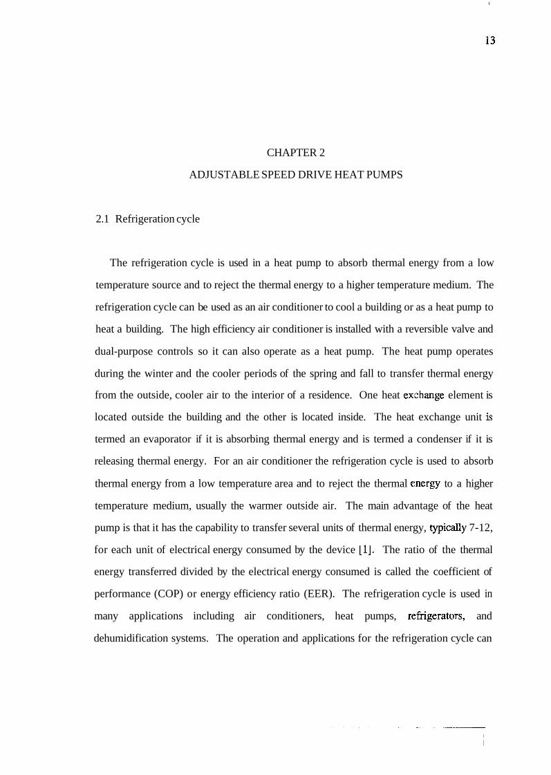
The refrigeration cycle is used in a heat pump to absorb thermal energy from a low
temperature source and to reject the thermal energy to a higher temperature medium. The
refrigeration cycle can be used as an air conditioner to cool a building or as a heat pump to
heat a building. The high efficiency air conditioner is installed with a reversible valve and
dual-purpose controls so it can also operate as a heat pump. The heat pump operates
during the winter and the cooler periods of the spring and fall to transfer thermal energy
from the outside, cooler air to the interior of a residence. One heat exlchange element is
located outside the building and the other is located inside. The heat exchange unit is
termed an evaporator if it is absorbing thermal energy and is termed a condenser if it is
releasing thermal energy. For an air conditioner the refrigeration cycle is used to absorb
thermal energy from a low temperature area and to reject the thermal energy to a higher
temperature medium, usually the warmer outside air. The main advantage of the heat
pump is that it has the capability to transfer several units of thermal energy, typically 7-12,
for each unit of electrical energy consumed by the device [I]. The ratio of the thermal
energy transferred divided by the electrical energy consumed is called the coefficient of
performance (COP) or energy efficiency ratio (EER). The refrigeration cycle is used in
many applications including air conditioners, heat pumps, rc:frigerators, and
dehumidification systems. The operation and applications for the refrigeration cycle can
be found in greater detail in references such as the Handbook of HVAC Design, [16], and
other references such as [lo], and [l 11.
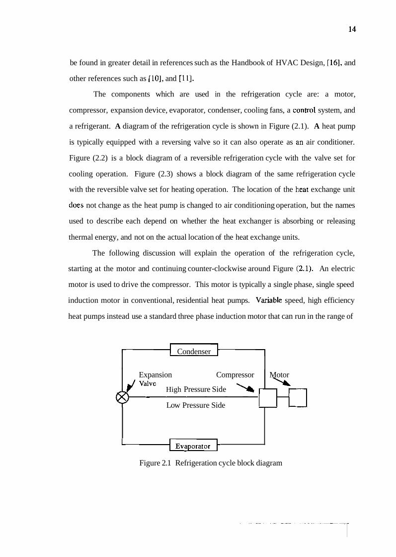
The components which are used in the refrigeration cycle are: a motor,
compressor, expansion device, evaporator, condenser, cooling fans, a control system, and
a refrigerant. A diagram of the refrigeration cycle is shown in Figure (2.1). A heat pump
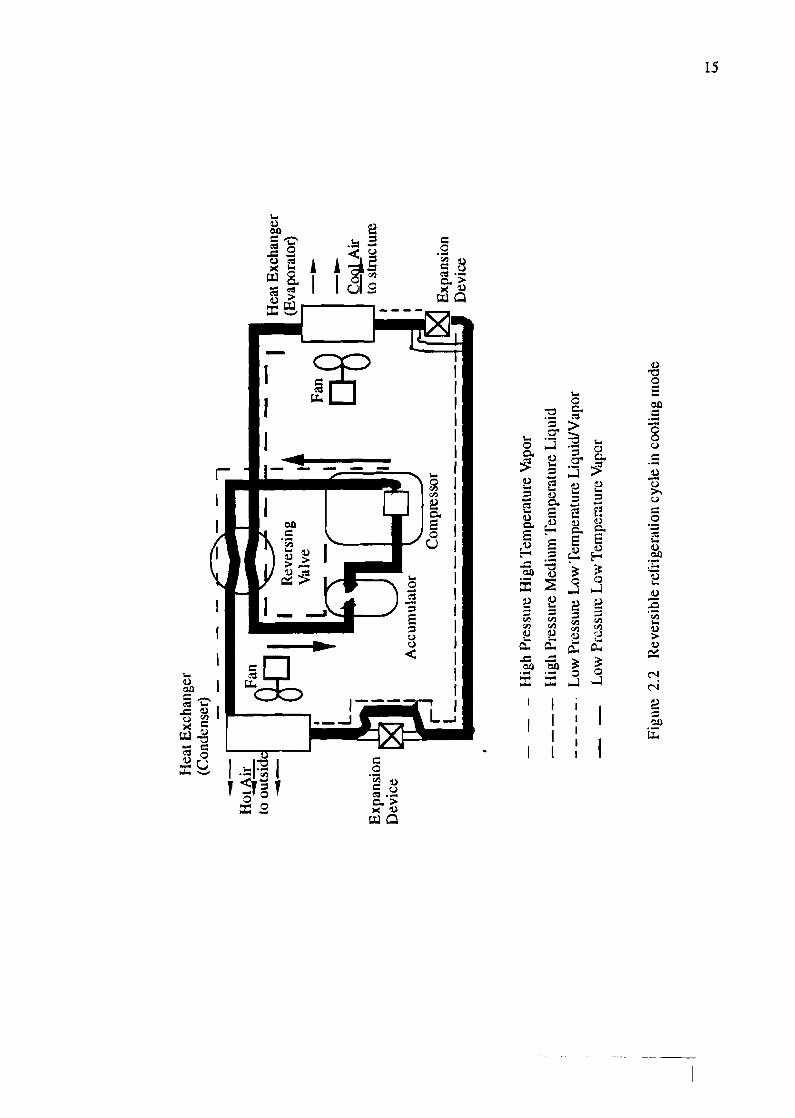
is typically equipped with a reversing valve so it can also operate as a.n air conditioner.
Figure (2.2) is a block diagram of a reversible refrigeration cycle with the valve set for
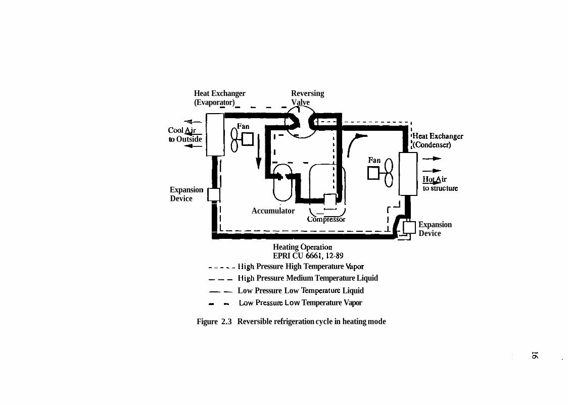
cooling operation. Figure (2.3) shows a block diagram of the same refrigeration cycle
with the reversible valve set for heating operation. The location of the h~eat exchange unit
does not change as the heat pump is changed to air conditioning operation, but the names
used to describe each depend on whether the heat exchanger is absorbing or releasing
thermal energy, and not on the actual location of the heat exchange units.
The following discussion will explain the operation of the refrigeration cycle,
starting at the motor and continuing counter-clockwise around Figure (2.1). An electric
motor is used to drive the compressor. This motor is typically a single phase, single speed
induction motor in conventional, residential heat pumps. Variable speed, high efficiency
heat pumps instead use a standard three phase induction motor that can run in the range of
Figure 2.1 Refrigeration cycle block diagram
Condenser
Expansion Compressor Motor
High Pressure Side \ 'i
Low Pressure Side - -11
Heat Exchanger Reversing (Evaporator) Valve
m - - -
1
Cool& to Outside - Expansion Device
I I Accumulator \ -1
Heating Opemtion EPRI CU 6661,12-89
- - - - - High Pressure High Temperature Vdpor --- High Pressure Medium Temperature Liquid
- - Low Pressure Low Temperdt ure Liquid - I. b w P r e s s u ~ Low Temperature Vapor
Y Expansion Device
Figure 2.3 Reversible refrigeration cycle in heating mode
about twenty percent to two hundred percent of rated speed for extended periods of time
[12]. The motor is connected directly to the compressor, and the motor and compressor
are usually enclosed in a common, sealed case. The compressor is used to pump the
refrigerant around the loop. The compressor also raises the pressure arid temperature of
the evaporated refrigerant as it pumps the refrigerant to the condenser. The temperature
of the refrigerant in the condenser is higher than the temperature of the medium, usually
air, around the condenser. This difference in temperature allows the condenser to reject,
or give off, heat to the surrounding medium. The refrigerant changes from a vapor to a
liquid in the condenser and heat is given off during this change in phase. A small motor is
used to drive a fan to increase the air flow through the condenser. This increased flow of
air across the heat exchanger increases the rate of energy transfer. 'The condenser is
constructed with narrow fins which provide extra radiating surface are:a to increase the
effective surface area used for energy transfer. During heat pump operation the heat
rejected by the condenser is used to warm the interior of a building. The condenser
releases thermal energy to the outside air during air conditioning operation.
After the liquid refrigerant leaves the condenser it passes through an expansion
device. The expansion device is simply a small restriction through which the refrigerant
passes. The expansion device can be connected to a control mechanism and is changed in
diameter in variable speed heat pumps. The refrigerant is changed from a high pressure,
medium temperature liquid into a low pressure, low temperature mixlure of vapor and
liquid. This decrease in the temperature of the refrigerant is due to the increased volume
that the refrigerant occupies, as evidenced by the lower pressure.
After leaving the expansion device the refrigerant next enters the: evaporator. The
temperature of the refrigerant is lower than the temperature of the medium, usually air,
surrounding the evaporator. This difference in temperature allows the refrigerant to
absorb thermal energy in the evaporator. The refrigerant will change phase from a mixture

of vapor and liquid into a vapor. Energy is absorbed by the evaporator d.uring this change
in phase from a liquid to a vapor. One of the heat exchange units is located inside the
building and one is located outside. These heat exchange units are termed the evaporator
if it is absorbing thermal energy and the condenser if it is releasing thermal energy. In heat
pump operation the evaporator is located outside the building and absorb:^ energy from the
cooler, outside air. During air conditioning operation the evaporator is :located inside the
building and absorbs energy from the cooler interior of the building. A fan is also used on
the evaporator to increase the rate of energy transfer. After leaving the evaporator the
warmer, liquid refrigerant flows back to the compressor, whereupon the cycle repeats.
2.2 Adjustable speed drive heat pumps
Most conventional residential heat pumps and air conditioners hl use today use a
230V, single phase induction motor. These classical designs used a motor speed of 1750
or 3000 revolutions per minute, and a few are designed to switch between these two
operating speeds [I]. Most operate at only one speed, and the compre:ssor is turning at
the same speed as the motor. The thermal output of the refrigeration cycle is proportional
to the compressor speed. Thus a conventional heat pump and air condi,tioner is either on
at the maximum pumping and thermal transfer rate or is idle. Heat pumps and air
conditioning units are designed for maximum output so that they can satisfy the thermal
requirements of the coolest or warmest days, respectively.
The full output of the heat pump or air conditioner is not requircd to maintain the
desired building temperature. Since the heat pump and air conditioning unit is typically
oversized so that it will perform well even during the brief periods of temperature
extremes, the unit will be required to frequently cycle on and off a large percentage of the
time. Extra energy is required as the motor is energized to return the c:omponents of the

refrigeration cycle to their operating temperature. This is because the temperature of the
coniponents such as the condenser, evaporator, and compressor have been returning to the
ambient, background temperature while the compressor is idle. The energy required to
bring components to the operating temperature each time the unit is cycled on is wasted
energy.
High efficiency, adjustable speed drive heat pumps are equipped with power
electronic circuits so that the motor can operate over a wide range of speed for long
periods of time [13]. A block diagram of an adjustable speed drive heat pump is shown in
Figure (2.4). Variable speed operation offers several advantages. The 'thermal output of
the heat pump and air conditioning unit is proportional to the speed (sf the motor and
conlpressor. The compressor speed can be varied so that the thermal output of the heat
pump and air conditioning unit more closely matches the energy that is required to
maintain the building at a constant temperature. With operation in this manner, the heat
pump can remain on for extended periods of time, which drastically reduces the cycling
losses. The motor will be run at slower speeds when the heating demand is low, and will
be run at high speeds for increased thermal output.
During a large portion of the operation of a heat pump or air corlditioning unit the
full thermal output of the unit will not be required. Therefore cycling losses can be
significant. The adjustable speed drive heat pump drastically reduces the cycling losses
since the unit remains on for much longer periods of time. If the heating demand is low
the compressor can be run at a fraction of its rated speed, which produces a lower flow
rate: in the refrigeration cycle. Besides the obvious advantage that the compressor requires
less energy to pump at a lower rate, the overall coefficient of performance increases as the
flow rate decreases. This inverse relationship between the coefficient of performance and
the flow rate occurs because the refrigerant stays in the evaporator and the condenser for
a longer period of time. The total amount of energy transferred in the evaporator or

condenser is greater with the slower flow rate since the refrigerant ;stays in the heat
exchange unit for a longer period of time. Thus the refrigerant has time to accept or reject
more thermal energy. The cooling fans can also be slowed down to consume less power
during periods of low thermal demand. During those periods when the full output of the
unit is required the compressor can be operated at a speed that is greater than the rated
speed of the motor. It is for these reasons that the adjustable speed drive has been
successfully applied to the refrigeration cycle to achieve significant energy savings. An
average energy savings of 15% is estimated for the adjustable speed drive: heat pump [:I.].


CHAPTER 3
MODELING OF THE ASD HEAT PUMP
3.1 Introduction
In this chapter, the components of an ASD heat pump are mocleled and studied.
Also, the supply distribution transformer is modeled. The objective is to assess the typical
impact of an ASD heat pump on power distribution systems. The chapter is organized
into five main topics, which include:
modeling of the electric motor
modeling of the power electronic drive
modeling of the distribution transformer
modeling of the compressor shaft load
ACSL program explanation and listing .
The Advanced Continuous Simulation Language (ACSL) will be useld to simulate the
combination of the above components. This chapter will provide a detailed derivation of
equations and an explanation of the method of operation of the csomponents to be
modeled. In addition, the last section contains the ACSL listing in sections, along with an
explanation of the purpose of each section.

3.2 Modeling of the electric motor
A three phase induction motor is typically used to drive the (compressor in an
adjustable speed drive heat pump. The three phase induction motor is more efficient and
is thus preferred over the single phase induction motor. Other high efficiency motors,
such as permanent magnet rotor machines, are also being considered for use in this
application. The efficiency of a motor can decrease with a decrease in motor speed. Since
a power electronically driven motor must operate over a wide range of speeds the
efficiency over the entire operating range must be considered to minimize: operating losses.
Although other motors can be used with adjustable speed drives, the three phase induction
motor is the most common for this application. Thus the induction motor will be modeled
in the simulation of the electric motor used in ASD heat pumps. This section will show
how the equations that describe the operation of an induction machine me derived.
The three phase induction machine consists of three sets of windings on the stator,
which is the outer stationary part of the motor and three sets of windings on the rotor.
Figure (3.1) shows the stator along with the rotor, which is the inner, rotating portion of
the motor. This frrst figure also shows how a conductor is placed lengthwise in the
machine. Typically one phase winding consists of many turns of insulated wire. The turns
which make up the winding are distributed along the stator as shown in :Figure (3.2). The
turns are distributed so that the air gap magneto-motive force (MMF) resulting from the
flow of current through the windings is sinusoidal. The voltage heumonics are also
minimized when the turns are distributed. Although the windings are ac:tually distributed,
it is; convenient for analysis to represent each set of windings as one equivalent conductor.

Stator I I Is -
I I
Rotor
I I 4
Figure 3.1 Side view of motor with stator winding
Figure (3.3) shows the cross-sectional view of a three phase induction motor,
where each phase winding is represented by one equivalent winding. The three phase
induction motor consists of the a, b, and c phase windings that are separated by 120
degrees from each other. These three windings on the stator would typically be connected
to a three phase voltage during operation. The rotor windings can also t~ represented as
three sets of windings, each separated from the other by 120 degrees. The rotor can
rotate with respect to the stator windings. The angle between the as axis and the ar axis is
given by &. The stator and rotor circuits of the induction machine can also be represented
as a balanced wye connected stator and rotor circuit consisting of a resistance and an
inductance in series. The analysis is more involved than would appear from Figure (3.4)
because there is mutual inductance between all of the inductors. In addition, the mutual
inductance between the stator and rotor inductances is a function of the rotor position.
The rotor position is also a function of time. A current flowing through a winding causes
a magnetic flux to flow in the motor. This flux will pass through the other windings of the

Wmding A Density
r
360 180
Figure 3.2 Winding turns density versus 8r
Figure 3.3 Cross-sectional view of induction motor showing the locations of the rotor and stator windings

machine to cause linkage between the windings.
The derivation of the machine equations for the three phase induction machine
involves six voltage equations: three for the stator and three for the rotor circuit. For
convenience and to make the equations more compact, matrix and vector notation will be
used. The notation used in this section follows that used by Krause in [5 ] . The (p)
operator will be used to denote the derivative operation with respect to time. The
machine voltage equations can be written as shown below. The first equation shows the
stator voltage equations in matrix form. The second equation shows the rotor voltage
equations in matrix form. The matrix notation used is shown in the third and fourth
equation for the stator and rotor, respectively,
Vabcs = rsm Iabcs + P A abcs
Vabcr = rrm Iabcr + P abcr
---.) ibs i r 4 -
7 var iarr-
Figure 3.4 Equivalent circuit of induction machine

1 f a r = [ f a r fbr f c r ]
The flux linkage, h, is written as an inductance times the current, as shown in
Equation (3.1) for the stator and rotor circuits. The stator, rotor, and rnutual inductance
matrices are also shown following Equation (3.1). The leakage inductance Lk and Llr
represents the flux produced by a stator or rotor winding, respectively, ithat does not link
with any other winding. The mutual inductances Lms and Lmr represent the flux linkage
produced by a winding that links with, or passes through, other windings. Since the
machine is assumed to be symmetric, these quantities are the same for thle stator and rotor 1 1
circuits. The - - L, and - - L, terms come about because the windings are 2 2
separated by 120 degrees in the stator and rotor. The flux produced by the stator also
links with the rotor windings and the flux produced by the rotor links with the stator
windings. The amount of flux linking the stator and rotor windings changes with the angle
between the stator and rotor. Hence the cos(8r) term occurs,
abcs (3.1)

In the analysis of a transformer the secondary parameters, such as the voltage,
current, and impedance, are typically referred to the primary by rr~ultiplying by the
appropriate turns ratio. In the same manner the analysis of the induction motor is made
easier if the rotor variables are referred through the turns ratio to stator variables. This is
done using the following equations for the current, voltage, flux linkage, and impedance
where primed variables have been referred to the stator windings,
&, = hr
-
COS (0 r ) cos (er + %) C O S ( ~ ~ - + )- cos [ er - - 2;) c o s ( e r ) cos (er + 5) cos (,, + $) cos (,, - F) cos ( 1 , )
- -
1
.

Gr = Ls
- cos (or ) cos [Or + +) cos [Or - 9) cos ( or - - Z;) cos(0r) cos + $1 cos [or + Zjl) cos (or - $) cos (0, )
- 2

The voltage equations are now written,
The implementation of the above voltage equation is difficult because it involves
the derivative of a product of two variables that are a function of fme, current and
inductance. A transformation to the arbitrary reference fiarne will make the analysis less
con~plicated. A transformation can be used to turn the time-varying mutual inductances
Lqsr to a constant. This is accomplished by the following arbitrary reference frame
transformation which converts the (abc) rotor variables to the (qdo) axis in the arbitrary
reference frame,
sin [p - 2)

Figure 3.5 Figure showing relationship between (abc) and (qdo) variables
2 &= - 3
sin(e) sin e - - ( ] s in[e+%) 1 - 1 - 1 - 2 2 2
L -
.

Figure (3.5) shows the relationship between the (abc) and qdo variables. When
this transformation is applied to the previously developed machine voltage Equation (3.2)
in the (abc) reference frame the following (qdo) equations result,

The voltage equations are now written in expanded form as shown below,
Each voltage equation now contains the derivative of only one variable, h so the
simulation of this set of equations is more straight-forward. These equations are valid for
any value of w, but the equations are simpler if the arbitrary reference frame velocity
equals zero. The ACSL simulation uses the stationary reference frame.

3.3 Modeling of the adjustable speed drive
3.3.1 Introduction
There are many types of ASD circuit topologies and switching strategies. Most
convert the input ac waveform to dc with a rectifier, then use an inverter to reconstruct an
ac waveform which is used to supply the machine. The voltage source inverter employs
one of the simplest switching strategies and has been favored because of the low switching
frequency requirements and its rugged design. Due to the low switching frequency the
rectifier and inverter switches are modeled as ideal. The disadvantages of the voltage
source inverter include poor power factor at low speeds and low speed pulsations [8].
The voltage source inverter is modeled in this simulation. The circuit diagram of the
voltage source inverter is shown in Figure (3.6) Each of the ten thyris1:ors are numbered
to facilitate later reference.
Figure 3.6 Voltage source inverter adjustable speed drive

The input is single phase ac and the three phase output voltage waveform is a six-
step waveform as shown in Figure (3.7). A silicon controlled rectifier (SCR) is used in the
rectifier. The SCR will conduct if it is forward biased and is subjected to either: gate
pulses, high forward voltages, transient voltage spikes, or high temperatures. During
normal operation the solid state switch will only turn on with the application of a current
to the gate terminal. The SCR will turn off if the current through it tries to reverse. The
rectifier uses an SCR so that the turn on point can be changed to control the dc voltage
produced. This is important so that a constant volts/hertz ratio can be maintained in the
induction motor. If the voltage applied to an induction machine is not reduced at lower
speeds, the machine flux will increase, which may cause saturation. The operation of the
voltage source inverter adjustable speed drive is explained in a subsequent section
describing the inverter. Also, an explanation of the operation of the rectifier is given.
Six step voltage waveform
Figure 3.7 Six step voltage waveform
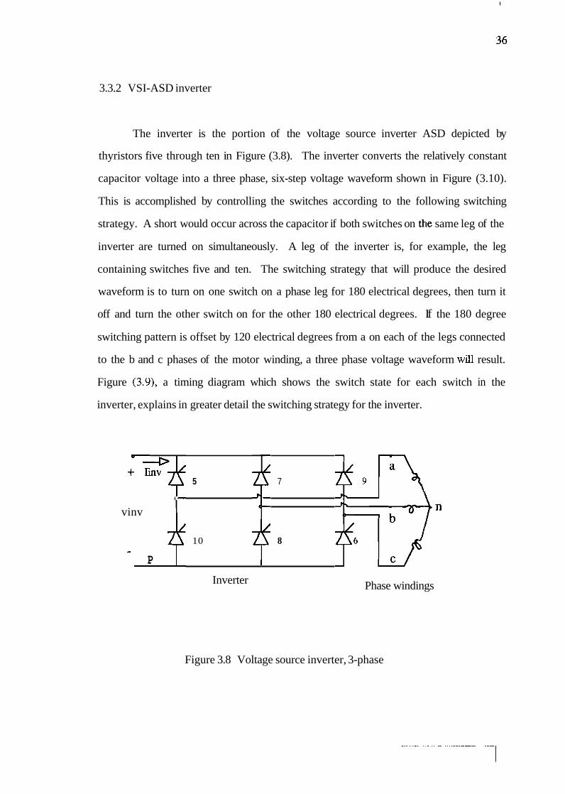
3.3.2 VSI-ASD inverter
The inverter is the portion of the voltage source inverter ASD depicted by
thyristors five through ten in Figure (3.8). The inverter converts the relatively constant
capacitor voltage into a three phase, six-step voltage waveform shown in Figure (3.10).
This is accomplished by controlling the switches according to the following switching
strategy. A short would occur across the capacitor if both switches on thle same leg of the
inverter are turned on simultaneously. A leg of the inverter is, for example, the leg
containing switches five and ten. The switching strategy that will produce the desired
waveform is to turn on one switch on a phase leg for 180 electrical degrees, then turn it
off and turn the other switch on for the other 180 electrical degrees. If the 180 degree
switching pattern is offset by 120 electrical degrees from a on each of the legs connected
to the b and c phases of the motor winding, a three phase voltage waveform will result.
Figure (3.9), a timing diagram which shows the switch state for each switch in the
inverter, explains in greater detail the switching strategy for the inverter.
5 7
4 8 b
vinv *
10 8 - P
Inverter Phase windings
Figure 3.8 Voltage source inverter, 3-phase
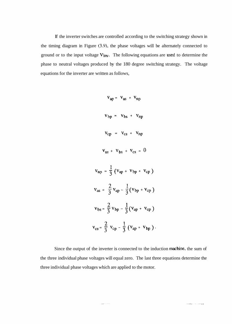
If the inverter switches are controlled according to the switching strategy shown in
the timing diagram in Figure (3.9), the phase voltages will be alternately connected to
ground or to the input voltage Vhv. The following equations are usedl to determine the
phase to neutral voltages produced by the 180 degree switching strategy. The voltage
equations for the inverter are written as follows,
Since the output of the inverter is connected to the induction machine, the sum of
the three individual phase voltages will equal zero. The last three equations determine the
three individual phase voltages which are applied to the motor.

7 Switch Number
Electrical 0 ~ / 3 21113 x 4x13 5x13 2~ 7x13 8x13 Radians
Figure 3.9 Inverter switching strategy

Vas
Vbs time
- vcs
time
Figure 3.10 Six step inverter waveform
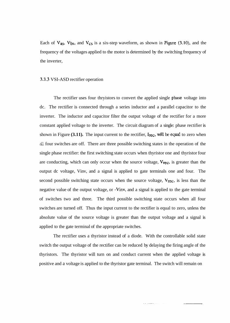
Each of Vas, Vbs, and Vcs is a six-step waveform, as shown in Figure (3.10), and the
frequency of the voltages applied to the motor is determined by the switching frequency of
the inverter,
3.3.3 VSI-ASD rectifier operation
The rectifier uses four thryistors to convert the applied single pbhase voltage into
dc. The rectifier is connected through a series inductor and a parallel capacitor to the
inverter. The inductor and capacitor filter the output voltage of the rectifier for a more
constant applied voltage to the inverter. The circuit diagram of a single: phase rectifier is
shown in Figure (3.1 1). The input current to the rectifier, Irec, will be equal to zero when
all four switches are off. There are three possible switching states in the operation of the
single phase rectifier: the first switching state occurs when thyristor one and thyristor four
are conducting, which can only occur when the source voltage, Vrec, is greater than the
output dc voltage, Vinv, and a signal is applied to gate terminals one and four. The
second possible switching state occurs when the source voltage, Vrec:, is less than the
negative value of the output voltage, or -Vinv, and a signal is applied to the gate terminal
of switches two and three. The third possible switching state occurs when all four
switches are turned off. Thus the input current to the rectifier is equal to zero, unless the
absolute value of the source voltage is greater than the output voltage and a signal is
applied to the gate terminal of the appropriate switches.
The rectifier uses a thyristor instead of a diode. With the controllable solid state
switch the output voltage of the rectifier can be reduced by delaying the firing angle of the
thyristors. The thyristor will turn on and conduct current when the applied voltage is
positive and a voltage is applied to the thyristor gate terminal. The switch will remain on

until the current through the device goes to zero. The equations which describe the
rectifier can be described in two sets: one set of equations when a rectifier thyristor is
conducting, and one set of equations for the case when the rectifier thyristors are off. The
following equations describe the operation of the rectifier when the thyristor is on,
The thyristor will turn off when the current through it goes to zero. The equations
which describe the operation of the rectifier during this portion of the voltage cycle are
found directly from the previous equations. Since the rectifier is off the current through
the inductor is now equal to zero. The current through the inductor will remain at zero
until the switch is turned on, which can be accomplished by setting the time derivative of
the current through the inductor, 11 to zero. When the switches of the rectifier are turned
off the output voltage is simply the exponentially decaying voltage across the capacitor Cf
as shown by the following equations,
Figure 3.1 1 Single phase rectifier with LC filter

3.4 Modeling of the distribution transformer
The distribution transformer consists of two windings on a laminated, usually iron
core. The distribution transformer is used to reduce the distribution voltages to the lower
voltages used by individual residential and commercial customers. Additional information
on the transformer is given in Section 1.4. The equations which describe the operation of
the transformer are written as follows. The voltage across the primiuy or secondary
winding is equal to the current through the winding times the winding resistance plus the
time derivative of the flux linkage, as shown in the following equations,

The previous equations describe the primary and secondary voltages. The
secondary parameters are referred to the primary using the primed quantities defined
above. The voltage equations defined above can be used to simulate the: operation of the
transformer with the flux linkage per second, Y , as the state variables in the simulation.
The flux linkages per second and the transformer currents can be defined as follows,
where Lml is equal to the mutual inductance,
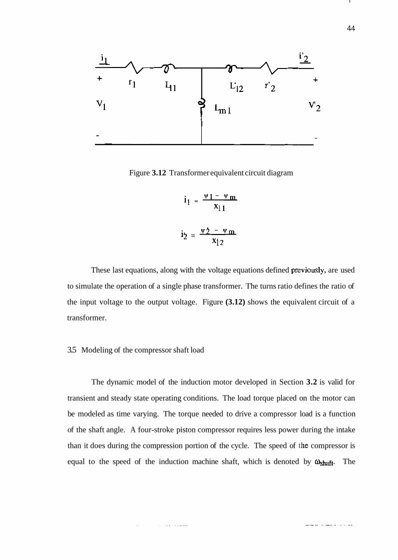
Figure 3.12 Transformer equivalent circuit diagram
These last equations, along with the voltage equations defined prc:viously, are used
to simulate the operation of a single phase transformer. The turns ratio defines the ratio of
the input voltage to the output voltage. Figure (3.12) shows the equivalent circuit of a
transformer.
3.5 Modeling of the compressor shaft load
The dynamic model of the induction motor developed in Section 3.2 is valid for
transient and steady state operating conditions. The load torque placed on the motor can
be modeled as time varying. The torque needed to drive a compressor load is a function
of the shaft angle. A four-stroke piston compressor requires less power during the intake
than it does during the compression portion of the cycle. The speed of rhe compressor is
equal to the speed of the induction machine shaft, which is denoted by %haft. The
compressor load is modeled as a constant value plus a sii~usoidally varyir~g quantity, which
accounts for the fact that the compressor load varies with position. This equation is,
Tcons tan t Tvar cos( shaft 2) .
The parameters of this equation can be changed to model the capacities and
characteristics of different compressors. This equation is only an estimate of the
compressor torque, as the time varying portion of the compressor torque is not sinusoidal.
3.6 ACSL program simulatio~l and listing
The Advanced Continuous Simulation Language, ACSL, will be used to simulate
the combination of the motor, drive, and distribution transformer. ACSL offers several
advantages over a general programming language. The ACSL program is simply a list of
the differential and algebraic equations which describe a system. The state variables are
those variables which are integrated to find the system behavior. The state variables are
entered as the time derivative of a state variable set equal to a function of the other state
variables or functions, as required for the model. ACSL allows one to choose from a
variety of pre-written integration algorithms, such as Runge-Kutta, Adams-Moulton, and
Gear's stiff, to find the solution to the state variables. One of the other main advantages of
ACSL is that the program will sort the equations, so they can be entered in any order.
ACSL also allows the user to change the model parameters while the simlulation is running
to aid in the simulation of a variety of system conditions. ACSL also allows for analysis
and plotting of the results of the simulation. The results of the ACSL s:imulation run can
also be transferred to Matlab for further analysis. Matlab is used to find the frequency
spectrum of selected model parameters.

The following ACSL program was written to simulate the single phase distribution
transformer, single phase rectifier, smoothing dc filter, three phase six-pulse inverter, and
three phase induction machine connected to a compressor load. The program Listing is
indented and will be separated into sections, preceded by an explanation of the purpose of
each main section.
The program statement is used to name the program. The ACSL program is
organized into blocks. The initial block is only executed once at the beginning of the
simulation run and is used to set the initial conditions, which end in -ic, of the state
variables. In this simulation all initial conditions are set to zero, except for Vinvic, which
is set to 200 volts. Any statement placed after an exclamation point in an ACSL program
is a comment statement, and will be left in this listing to facilitate the e.xplanation of the
program.
program vector initial ! induction motor state variable initial conditions Siqssic = 0.0 Sidssic = 0.0 Siqrsic = 0.0 Sidrsic = 0.0 wric= 0.0 ! transformer state variable initial conditions Silpric = 0.0 Si2ic = 0.0 ! control ramp signal initial conditions rampic = 0.0 ramppic = 0.0 ! smoothing LC filter initial conditions Vinvic = 200. ilic = 0.0 ! base frequency=377rad/sec wb = 2*60*3.14159 we = wb twopi = 2*3.14159
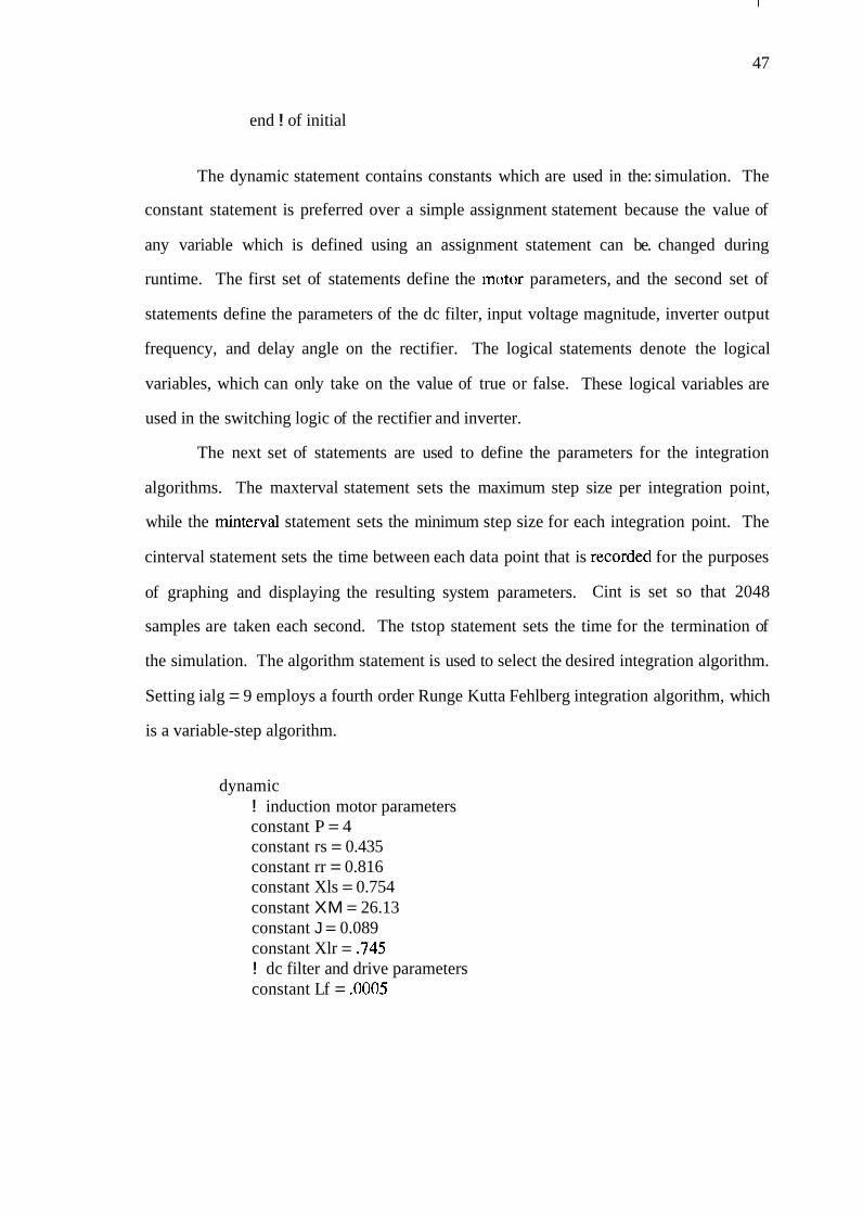
47
end ! of initial
The dynamic statement contains constants which are used in the: simulation. The
constant statement is preferred over a simple assignment statement because the value of
any variable which is defined using an assignment statement can be. changed during
runtime. The first set of statements define the motor parameters, and the second set of
statements define the parameters of the dc filter, input voltage magnitude, inverter output
frequency, and delay angle on the rectifier. The logical statements denote the logical
variables, which can only take on the value of true or false. These logical variables are
used in the switching logic of the rectifier and inverter.
The next set of statements are used to define the parameters for the integration
algorithms. The maxterval statement sets the maximum step size per integration point,
while the rninterval statement sets the minimum step size for each integration point. The
cinterval statement sets the time between each data point that is recorded for the purposes
of graphing and displaying the resulting system parameters. Cint is set so that 2048
samples are taken each second. The tstop statement sets the time for the termination of
the simulation. The algorithm statement is used to select the desired integration algorithm.
Setting ialg = 9 employs a fourth order Runge Kutta Fehlberg integration algorithm, which
is a variable-step algorithm.
dynamic ! induction motor parameters constant P = 4 constant rs = 0.435 constant rr = 0.816 constant Xls = 0.754 constant XM = 26.13 constant J = 0.089 constant Xlr = .745 ! dc filter and drive parameters constant Lf = .0005

constant Cf = 0.01 constant Vmag = 250 constant Fme = 40. constant alpha = .Ol ! transformer parameters constant r l = .25 cons tan t r2pr = .I34 constant xmtran = 708.8 constant x l 1 = .056 constant xl2pr = .056 Ntrans = 1.0 constant Rload = 100 logical SA, SB, SC logical gtzero logical Ron ! ACSL integration parameters maxterval maxt = 2E-6 minterval mint = 1E-6 cinterval cint = 4.882E-4 constant tstop = .2 termt (t.gt.tstop) algorithm ialg = 9 merror wr = 1E-3 xerror wr = 1E-2
The derivative block contains the system equations which are evaluated at each
time step. All variables which are the derivatives of time are denoted by the p- prefix.
The first section contains the equations which describe the three phase induction machine.
These equations were described in detail in Section 3.2.
DERIVATIVE Tm = 1 ./Fme ! inverter output voltage period Vng = (Vag + Vbg + Vcg)/3.0 Vas = Vag - Vng Vbs = Vbg - Vng Vcs = Vcg - Vng Vab = Vas - Vbs vqss = (2./3.)*(Vas-0.5*Vbs-0.5*Vcs) vdss = (2./3.)*0.86602*(-Vbs+Vcs) vqrs = 0.0 vdrs = 0.0
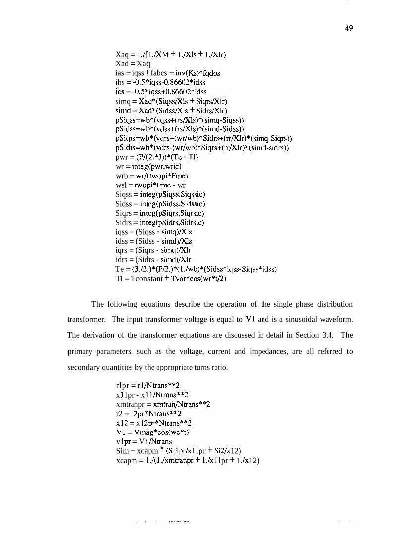
Xaq = 1 ./(I ./XM + l./Xls + l./Xlr) Xad = Xaq ias = iqss ! fabcs = inv(Ks)*fqdos ibs = -0.5*iqss-0.86602*idss ics = -0.5*iqss+0.86602*idss simq = Xaq*(Siqss/Xls + Siqrs/Xlr) sirnd = Xad*(Sidss/Xls + Sidrs/Xlr) pSiqss=wb*(vqss+(rs/Xls)*(simq-Siqss)) pSidss=wb*(vdss+(rs/Xls)*(simd-Sidss)) pSiqrs=wb*(vqrs+(w~/wb)*Sidrs+(rr/Xlr)*(simq-Siqrs)) pSidrs=wb*(vdrs-(wr/wb)*Siqrs+(rr/Xlr)*(simd-sidrs)) pwr = (P/(2.*J))*(Te - T1) wr = integ(pwr,wric) wrb = wr/(twopi*Fme) wsl = twopi*Fme - wr Siqss = integ(pSiqss,Siqssic) Sidss = integ(pSidss,Sidssic) Siqrs = integ(pSiqrs,Siqrsic) Sidrs = integ(pSidrs,Sidrsic) iqss = (Siqss - simq)/Xls idss = (Sidss - simd)/Xls iqrs = (Siqrs - simq)/Xlr idrs = (Sidrs - simd)/Xlr Te = (3./2.)*(P/2.)*(1 ./wb)*(Sidss*iqss-Siqss*idss) TI = Tconstant + Tvar*cos(wr*t/2)
The following equations describe the operation of the single phase distribution
transformer. The input transformer voltage is equal to V1 and is a sinusoidal waveform.
The derivation of the transformer equations are discussed in detail in Section 3.4. The
primary parameters, such as the voltage, current and impedances, are all referred to
secondary quantities by the appropriate turns ratio.
rlpr = rl/Ntrans**2 x 1 lpr - x 1 l/Ntrans**2 xmtranpr = xmtran/Ntrans**2 r2 = r2pr*Ntrans**2 x12 = x 12pr*Ntrans**2 V1 = Vmag*cos(we*t) v lpr = V l/Ntrans Sim = xcapm * (Silprlx 1 lpr + Si2Ix 12) xcapm = 1 ./(l ./xmtranpr + l./x 1 lpr + 1 ./x 12)

ilpr = (Silpr - Sim)/xllpr i l = ilprmtrans i2 = (Si2 - Sim)/xl2 V2 = -Rload*(iltran + i2) pSilpr = wb*(vlpr - rlpr*((Silpr psi2 = wb*(V2-r2*i2) Silpr = integ(pSilpr,Silpric) Si2 = integ(pSi2,Si2ic) Vm = 10*cos(twopi*t/Tm)
Sim)/x 1 1 pr))
The following equations are used to model the dynamics of the series inductor and
parallel capacitor which is used to filter the output of the rectifier. Tllis provides for a
more constant input voltage to the inverter. Vinv is used to denote the voltage across the
capacitor and il denotes the current through the inductor. Since the input rectifier
converts the negative applied voltage to a positive voltage, the derivative of the inductor
current must be defined with two different equations. The variable pilonplus is used when
the input rectifier voltage is greater than zero, and the variable pilonmns is used when the
input rectifier voltage is less than zero. The RSW switch is used to set the value of pilon,
which applies when the rectifier switches are on. The variable pil is equal to pilon when
the rectifier is on, and is set equal to zero when the rectifier is turned off.
pVinv = (l./Cf)*(il - Iinv) Vinv = integ(pVinv,Vinvic) pilonplus = (l./Lf)*(Vrec - Vinv) pilonrnns = ( 1 ./Lo*(-Vrec-Vinv) pilon = RSW(gtzero,pilonplus,pilonmns) pi1 = RS W(Ron,pilon,O.O) il = integ(pi1,ilic) Vrec 1 = Vmag*(3./4.)*cos(we*t) Vrec = V2pr schedule commute .XN. il ! sets Pi1 to zero when I1 = 0
The inverter output voltage waveform depends on the switching pattern of the
inverter. This simulation includes a controller that controls the inverter switches
according to the timing diagram shown in Fig. (3.9). A ramp function with a period equal

to the inverter output voltage is defined in the following sections by the variable ramp.
The ramp function is used because it is convenient to determine the position in the cycle
for switching purposes. 'The variable rampp defines a ramp function with a frequency
equal to the input voltage and is used in the rectifier switching logic. A procedural block
is executed at every time step of the simulation run. The following procedural blocks are
necessary since the negative applied voltage is turned around by the rectifier switches.
The current through the smoothing inductor is always greater than or equal to zero, while
the input current is positive when the applied voltage is greater than zero, and is negative
when the applied voltage is negative.
pramp= 1.0 ramp=integ(pramp,rampic) schedule zero .XP. Vm ! sets ramp to zero prampp = 1.0 rampp = integ(prarnpp,ramppic) schedule zeroo .XZ. Vrecl ! sets rampp to zero
procedural(iltran=il,Vrecl) if(Vrecl.lt.0.) iltran = -il if(Vrec1 .gt.O.) iltran = il
end
procedural(gtzero=Vrec) ! flag = .t. if VreoO if(Vrec.gt.0.) gtzero=.true. if(Vrec.lt.0.) gtzero=.false.
end
procedural(Ron=rampp,Vrec,alpha) if(Vrec.lt.0) Vrecc = - Vrec if(Vrec.gt.0) Vrecc = Vrec if((rampp.gt.alpha/6O.).and.(Vrecc.gt.Vinv)) Ron = .true.
end ! of procedural to determine rectifier turn-on time
procedural(Vag,Vbg,Vcg=Vinv,S A ,SB,SC) Vag = 0 Vbg = 0 vcg = 0 if(SA) Vag = Vinv

if(SB) Vbg = Vinv if(SC) Vcg = Vinv
end ! of procedural to determine inverter voltages
procedural(Iinv=S A,SB,SC,ias,ibs,ics) Iinv = 0.0 if(SA) Iinv = ias if(SB) Iinv = Iinv + ibs if(SC) Iinv = Iinv + ics
end ! of procedural to calculate inverter current Iinv procedural(S A,SB,SC=ramp,Tm) ! This procedural block controlls the switch states, SA, ! SB, SC to produce a six-step output voltage waveform SA = .false. if((ramp-(Tm/2.)).1t.O) SA = .true. SB = .false. i f ( ( r a m p . l t . ( 5 . * T m / 6 . ) ) . a n d . ( r a m p . g t . ( T ~ u e . SC = .false. if((ramp.gt.(2.*Tm/3.)).or.(ramp.lt.(Tm/6.)))SC=.true. end ! of procedural end ! of derivative
A discrete block is executed whenever directed by the schedule operator. The
following blocks are used to set the ramp functions to zero at the approlpriate times. The
discrete block named commute is used to turn off the rectifier switches. Each block must
be concluded with an end statement.
discrete zero ramp=0.0
end ! of discrete to re-set the inverter ramp to zero discrete zeroo
rampp = 0.0 end ! of discrete to re-set the rectifier ramp to zero discrete commute ! this block switches from Vcon to Vcoff if Ron is .true.
if(Ron) Ron = .false. end ! of discrete end ! of dynamic end ! of program
Figure (3.13) is a block diagram of the transformer and drive modeled by the
ACSL program with program variables labeled.

CHAPTER 4
SIMULATION RESULTS AND ANALYSIS
4.1 Introduction
The ACSL program which simulates the transient and steady state operation of the
distribution transformer, six step voltage source inverter adjustable speed drive, three
phase induction motor, and compressor load is described in detail in Section 3.6.
Simulation output for various operating conditions is presented in this chapter. These
figures illustrate the operating characteristics of the motor and drive combination. Also,
the figures clearly show the characteristics of the voltage supplied to and the current
drawn by the drive. These figures were obtained by transferring the prepared variables
from ACSL to Matlab for plotting the variables as a function of time or frequency. To
determine the harmonic content of selected waveforms, the fast Fourier transform (FFT)
Matlab command was used to obtain the frequency spectrum of selected waveforms. The
input rectifier current and the inverter output voltage waveforms h~ave a significant
harmonic content.
The parameters used in the simulation are given in the ACSL program listing in
Section 3.6. The induction motor parameters are for an induction motor with rated values
of 220 volts, 3 horsepower, and 1710 rpm were taken from [20]. The transformer
parameters are for a 240/120V, single phase transformer [21]. The values for the
smoothing filter between the rectifier and inverter were chosen so that the current through
the inductor and the voltage across the capacitor would not change too rapidly or too

slowly to yield undesired simulation output waveforms. In an actual system the
parameters of the drive would be determined by other factors. The switches in the
rectifier and inverter are modeled as ideal: they are either on or off, can be switched
instantaneously, and have a zero forward voltage drop. The ideal switch approximation is
justified because of the low switching speeds in the voltage source inverter and the single
phase rectifier.
As discussed in Section 1.4.4, ANSI C57.110 provides a method which can be
used to determine the transformer derating when supplying nonsinusoidal loads. The
hannonic content of the input currents drawn by the drive and motor in the simulation are
used to determine the transformer derating, assuming that the transformer is loaded to its
full capacity with all ASD and one half ASD loading levels. Also, plots taken from an
actual, installed heat pump are included for qualitative comparison t~o the wavefonns
produced by the simulation. The plots cannot be directly compared to the simulation
results because the parameters of the measured system were not available:. The derating of
the distribution transformer for the actual installation is also presented. The total
hannonic distortion, THD, is also calculated for the primary and secondary transformer
current. Also, the IEEE Standard 519-1992, which includes recommended limits on the
current distortion for individual consumers of electric energy, is presented. The total
harmonic distortion of the simulated and measured current wavefo~rms are used to
determine if the IEEE Standard 519-1992 limits are violated in either case.
4.2 Simulation results
The ACSL simulation is valid for transient and steady state operating conditions.
Several cases are presented to show the operation of the system during startup and steady
state conditions for zero applied load torque, a simulated compressor load, and step
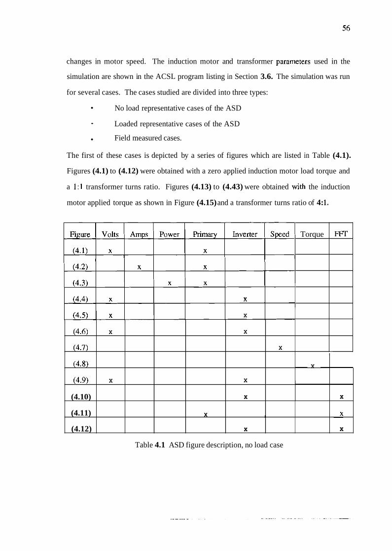
changes in motor speed. The induction motor and transformer parameters used in the
simulation are shown in the ACSL program listing in Section 3.6. The simulation was run
for several cases. The cases studied are divided into three types:
No load representative cases of the ASD
• Loaded representative cases of the ASD
Field measured cases.
The first of these cases is depicted by a series of figures which are listed in Table (4.1).
Figures (4.1) to (4.12) were obtained with a zero applied induction motor load torque and
a 1:l transformer turns ratio. Figures (4.13) to (4.43) were obtained with the induction
motor applied torque as shown in Figure (4.15) and a transformer turns ratio of 4: 1.
Table 4.1 ASD figure description, no load case
FFT
-
Torque
X
(4.6)
(4.7)
(4.8)
(4.9)
(4.10)
(4.11)
(4.12)
X
X
I
X
I x
X
X
x
x
I
P X
P
x
x
x

Figure (4.1) shows the transformer primary applied sinusoidal voltage. Figure
(4.2) shows the transformer input current, which clearly shows the nonsinusoidal current
drawn by the ASD. Figure (4.3) shows the instantaneous powr:r drawn by the
transformer. Figures (4.4), (4.9, and (4.6) show the six-step, three phase inverter output
voltages for the a, b, and c phase, respectively. Note that the frequency of the inverter
output voltage is equal to 40 hertz. Figures (4.7), (4.8), and (4.9) show the induction
motor rotor speed, electrical torque, and inverter applied voltage versus ti me, respectively.
Figure (4.10) shows the frequency spectrum of the six step inverter output voltage. Note
that the inverter fundamental frequency fo is 40 hertz, and the harmonic components are
present at (6h-l)fo and (6h+l)fo, where fo is the frequency of the fundamental component
and h is an integer. Figure (4.11) shows the frequency spectrum of the secondary current
through the transformer. Note that the frequency spectrum of the current drawn by the
ASD contains odd harmonics. Figure (4.12) shows the frequency spectrum of the current
drawn by the induction motor. The frequency spectrum of the current drawn by the
induction motor has components at the same frequency as the inverter output voltage
shown in Figure (4.10).
The loaded cases are also depicted by the figures which are listed in Table (4.2).
Figures (4.13) through (4.43) were obtained from the simulation of the ASD system with
the applied load torque shown in Figure (4.15). Figure (4.13) shows tht: induction motor
speed, which decreases as the load torque is increased. Figure (4.14) shlows the induction
motor electrical torque, which increases with the applied load torqut:. Figure (4.16)
shows the transformer secondary current, which is large during motor startup, and then
increases as the applied load torque increases. Figure (4.17) shows the transformer
primary instantaneous power, which increases as the load torque is increased. Figure
(4.18) shows the inverter input voltage, which decreases slightly as the load torque is
increased.

Table 4.2 Simulated motor load torque cases
Load number Figure Time interval Percent load
0
25
Expanded views of selected steady state power, current, and frequency spectrum
waveforms resulting from the five load torque levels shown in Figure (4.15) are presented
in Figures (4.19) to (4.43).
Table (4.2) gives the figure numbers associated with each load case. The five
figures shown for each of the five cases are the transformer primary current, secondary
current, primary power, frequency spectrum of transformer secondary current, and the
frequency spectrum of the transformer primary current. The frequency spectrum plots are
normalized so that the amplitudes are displayed as the percentage of the fundamental.
This is more convenient since the per unit values are needed for the transformer derating
calculations. As the load torque is increased, the current drawn by thle ASD increases.
Also, the current waveform becomes more sinusoidal as the input curren~t becomes larger.
Also, the transformer primary current is more sinusoidal than the secondary current
because of the filtering effects of the transformer.
3
4
5
(4.29) to (4.33)
(4.34) to (4.38)
0
1.5 - 2 seconds
2 to 2.5 seconds
5 0
75
100

Figure 4.1 Transformer primary voltage versus ' time
Figure 4.2 Transformer input current versus time
Figure 4.3 Transformer instantaneous power versus time
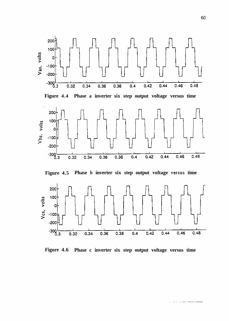
Figure 4.4 Phase a inverter six step output voltage versus time
Figure 4.5 Phase b inverter six step output voltage versus time
Figure 4.6 Phase c inverter six step output voltage versus time

Figure 4.7 Induction motor speed versus time
-200; 0.1 I 0.2 I I I I
0.3 0.4 0.5
Figure 4.8 Induction motor electrical torque versus time
Figure 4.9 Inverter input voltage Vinv versus time
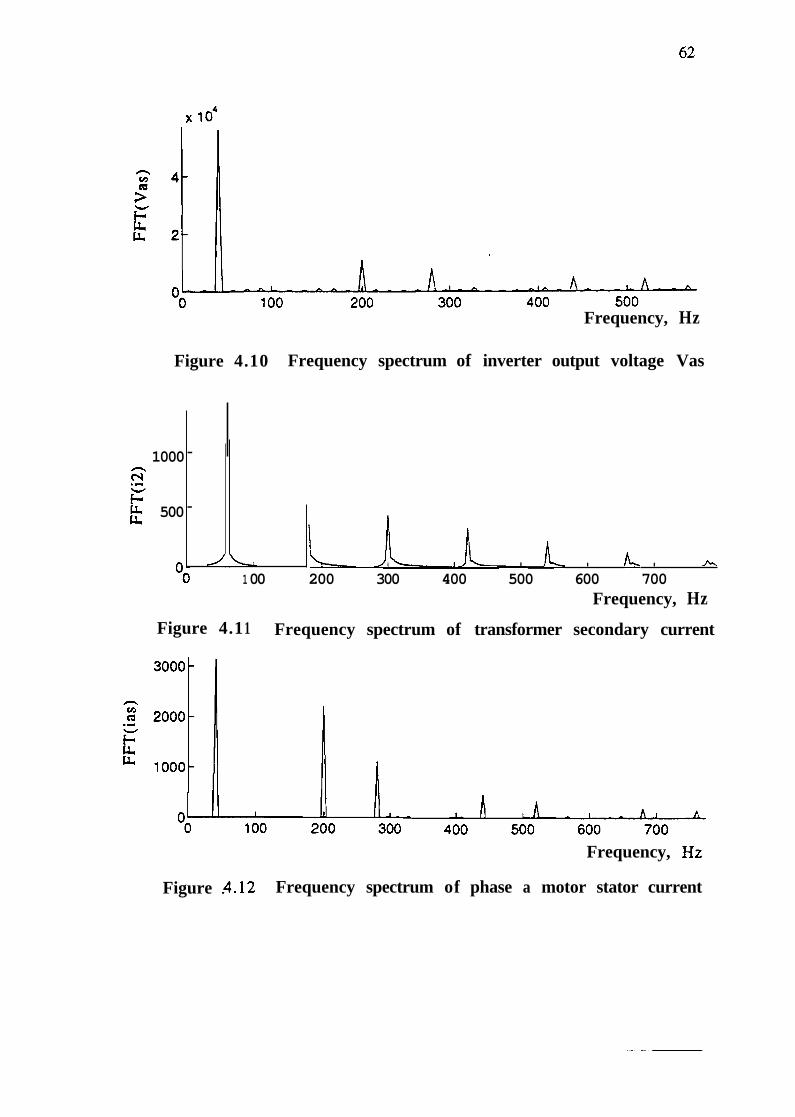
Frequency, Hz
Figure 4.10 Frequency spectrum of inverter output voltage Vas
Figure 4.1 1 Frequency spectrum of transformer secondary current
1000
500
Frequency, Hz
Figure -4.12 Frequency spectrum of phase a motor stator current
O* JL I I I I A
1 00 200 300 400 500 600 700 Frequency, Hz
-
- ,
j

Figure 4.13 Induction motor speed versus time
Figure 4.14 Induction motor electrical torque versus time
Figure 4.15 Applied load torque versus time

50
2 co 0
Pi- .- -50
Figure 4.16 Transformer secondary current versus time
Figure 4.17 Transformer primary ins tan taneous power versus time
Figure 4.18 Inverter input voltage versus time -
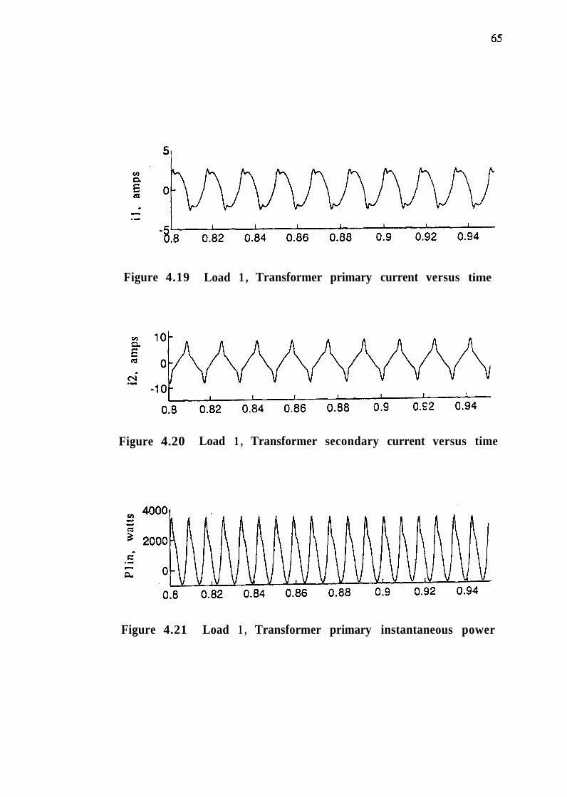
Figure 4.19 Load 1 , Transformer primary current versus time
Figure 4.20 Load 1 , Transformer secondary current versus time
Figure 4.21 Load 1 , Transformer primary instantaneous power

Frequency, Hz
Figure 4.22 Load 1 , Frequency spectrum of transformer secondary current expressed as a percentage of the fundnmenta.1
Figure 4.23 Load 1 , Frequency spectrum of transformer primary current expressed as a percentage of the fundamental
100r
83
@ - 60- yr C . -
40- L
20
-
-
OF I I A. I
100 200 300 400 500 600 Frequency, Hz
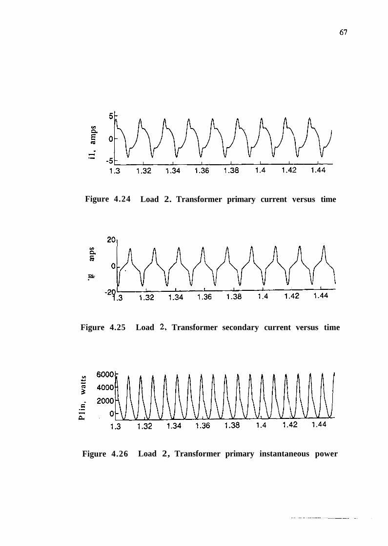
Figure 4.24 Load 2. Transformer primary current versus time
Figure 4.25 Load 2 , Transformer secondary current versus time
cn
P 'J
Pi- .-
Figure 4.26 Load 2, Transformer primary instantaneous power
0 - . /k'wNY%M

Frequency, Hz
Figure 4.27 Load 2 , Frequency spectrum of transformer secondary current expressed as a percentage of the fundamental
Frequency, Hz
Figure 4.28 Load 2, Frequency spectrum of transformer primary current expressed as a percentage of the funclamental
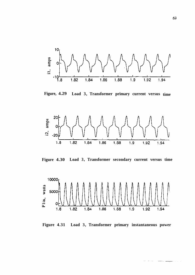
Figure, 4.29 Load 3, Transformer primary current versus time
Figure 4.30 Load 3 , Transformer secondary current versus time
Figure 4.31 Load 3 , Transformer primary instantaneous power

Frequency, Hz
Figure 4:32 Load 3 , Frequency spectrum of transformer secondary current expressed as a percentage of the fundamental
Frequency, Hz
Figure 4.33 Load 3 , Frequency spectrum of transformer primary current expressed as a percentage of the fundamental
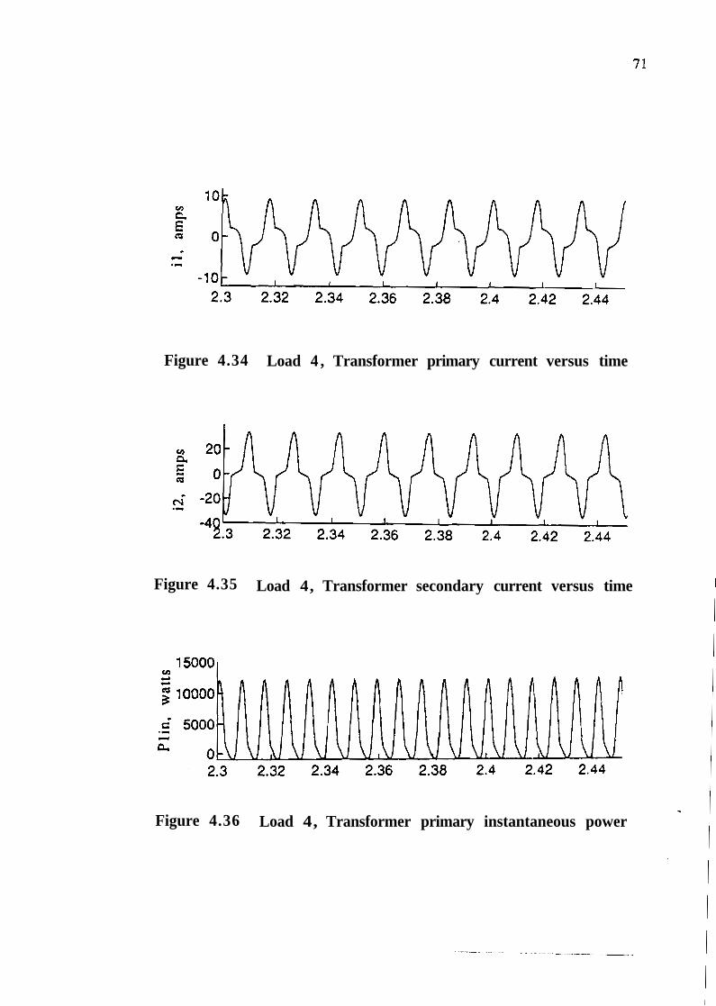
Figure 4.34 Load 4 , Transformer primary current versus time
Figure 4.35 Load 4, Transformer secondary current versus time
Figure 4.36 Load 4, Transformer primary instantaneous power

Frequency, Hz
Figure 4.37 Load 4 , Frequency spectrum of transformer secondary current expressed as a percentage of the fundilmental
Frequency, Hz
Figure 4.38 Load 4, Frequency spectrum of transformer primary current expressed as a percentage of the fundamental
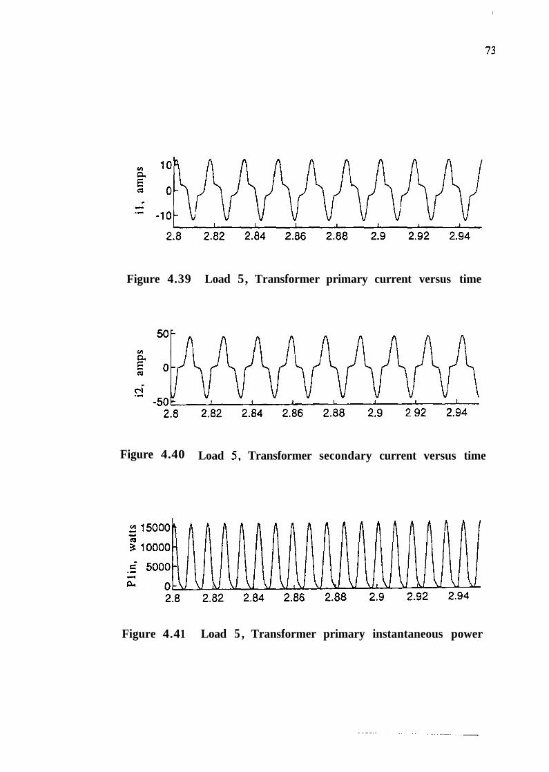
Figure 4.39 Load 5, Transformer primary current versus time
Figure 4.40 Load 5 , Transformer secondary current versus time
Figure 4.4 1 Load 5 , Transformer primary instantaneous power
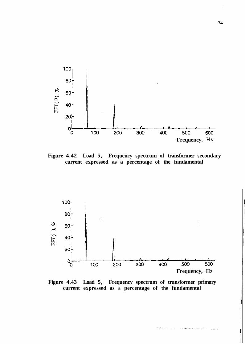
Frequency. Hz
Figure 4.42 Load 5, Frequency spectrum of transformer secondary current expressed as a percentage of the fundamental
Frequency, Hz
Figure 4.43 Load 5, Frequency spectrum of transformer primary current expressed as a percentage of the fundamental
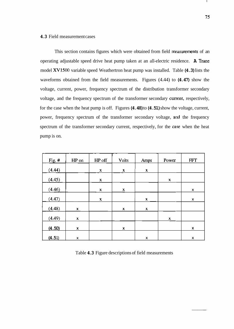
4.3 Field measurement cases
This section contains figures which were obtained from field measurements of an
operating adjustable speed drive heat pump taken at an all-electric residence. A Trane
model XV1500 variable speed Weathertron heat pump was installed. Table (4.3) lists the
waveforms obtained from the field measurements. Figures (4.44) to (4.47) show the
voltage, current, power, frequency spectrum of the distribution transformer secondary
voltage, and the frequency spectrum of the transformer secondary cunient, respectively,
for the case when the heat pump is off. Figures (4.48) to (4.51) show the voltage, current,
power, frequency spectrum of the transformer secondary voltage, and the frequency
spectrum of the transformer secondary current, respectively, for the case when the heat
pump is on.
Table 4.3 Figure descriptions of field measurements
FFT
X
X
x
X
(4.50)
(4.5 1)
x
X
x
X

Figure 4.44 Phase a current and voltage snapshot, heat pump off
Figure 4.45 Phase a instantaneous power. heat pump off
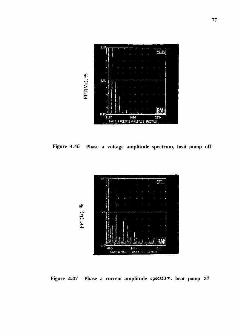
Figure .4.46 Phase a voltage amplitude spectrum, heat pump off
Figure 4.47 Phase a current amplitude spectrum. heat pump off
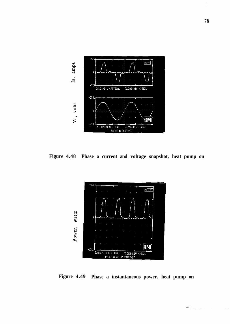
Figure 4.48 Phase a current and voltage snapshot, heat pump on
Figure 4.49 Phase a instantaneous power, heat pump on

Figure 4.50 Phase a voltage amplitude spectrum, heat pump on
Figure 4.51 Phase a current amplitude spectrum, heat pump on

4.4 Transformer derating calculations
4.4.1 ANSI C57.110 example calculation
The distribution transformer incurs additional losses when it is supplying harmonic
currents, as is the case for both the simulation results and the measured waveform
obtained from an actual installation. The ANSI C57.110 Standard is used to determine
the transformer derating, or reduction in power transfer capability, due to the flow of
harmonic currents [2]. This recommended practice has been described in more detail in
Section 1.4.4. The equation which determines the transformer derating is shown below.
To aid in the explanation of the calculation of the transformer derating, the following
example is included, which was taken from ANSI C57.110. The harmonic current
spectrum and other calculations are shown in Table 4.4. The variable fh is the ratio of the
harmonic current magnitude divided by the magnitude of the fundamental component of
current. The current magnitudes are all given in per unit quantities. The transformer
winding eddy-current loss density ( P ~ ~ a ( p u ) ) is 15% of the local I~R loss, therefore
PLL-R(PU) = 1.15 pu,

Table 4.4 ANSI C57.110 transformer derating example:
A transformer which is supplying current at the given magnitude of harmonic
component has a capability which is only 90.3% of the full-load rated value. Thus the
transformer is not able to transmit its full rated power due to the current harmonics drawn
by the load. A transformer that will supply a load that produces harmcllnic currents must
be oversized to ensure that the transformer temperature does not exceed design limits.
4.4.2 Transformer derating of actual system
The waveforms presented in Section 4.3 were obtained from an operating heat
pump. Table 4.5 gives the magnitude of each current harmonic and other calculations that
are needed to evaluate the derating. The transformer derating is calculated to be equal to
0.9368 in this case,
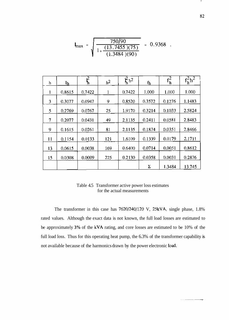
Table 4.5 Transformer active power loss estimates for the actual measurements
The transformer in this case has 7620/240/120 V, 25kVA, single phase, 1.8%
rated values. Although the exact data is not known, the full load losses are estimated to
be approximately 3% of the kVA rating, and core losses are estimated to be 10% of the
full load loss. Thus for this operating heat pump, the 6.3% of the transformer capability is
not available because of the harmonics drawn by the power electronic lo~id.

4.4.3 Transformer derating for simulation results
The waveforms produced by the simulation of the single phase transformer, drive,
and induction motor are shown in Section 4.2. The transformer secondary current
spectrum for the simulation results are shown in Figures (4.22), (4.27), (4.32), (4.37), and
(4.42). Each figure is the frequency spectrum for a different applied motor torque. Each
frequency spectrum shows that the transformer secondary current contains a significant
percentage of odd harmonics. The ANSI C57.110 Standard is used to calculate the
transformer derating for the simulation results. The root mean squared value of the
current containing harmonics, Ih, through the transformer is assumed tlo be equal to the
transformer rated current, thus the sum of Ih is equal to 1.0 per unit of the transformer
rating. This assumption may not be valid for the partial load cases, since if the ASD is
partially loaded, the transformer will not be fully loaded. Also, the transformer winding
eddy-current loss density is assumed to be 15% of the local copper loss. Table 4.6
contains the data taken from Figure (4.32), which is load 3 case.
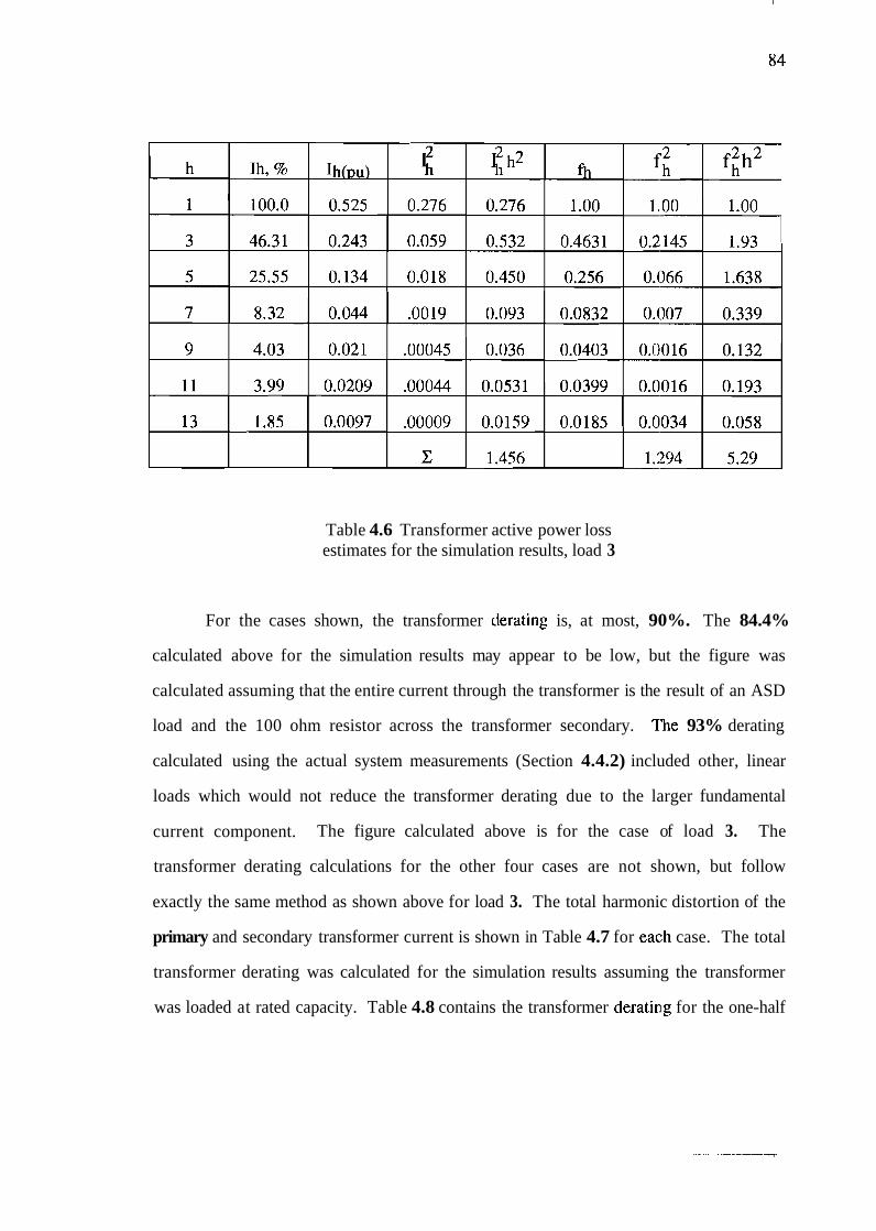
Table 4.6 Transformer active power loss estimates for the simulation results, load 3
For the cases shown, the transformer derating is, at most, 90%. The 84.4%
calculated above for the simulation results may appear to be low, but the figure was
calculated assuming that the entire current through the transformer is the result of an ASD
load and the 100 ohm resistor across the transformer secondary. The 93% derating
calculated using the actual system measurements (Section 4.4.2) included other, linear
loads which would not reduce the transformer derating due to the larger fundamental
current component. The figure calculated above is for the case of load 3. The
transformer derating calculations for the other four cases are not shown, but follow
exactly the same method as shown above for load 3. The total harmonic distortion of the
primary and secondary transformer current is shown in Table 4.7 for each case. The total
transformer derating was calculated for the simulation results assuming the transformer
was loaded at rated capacity. Table 4.8 contains the transformer deratin~g for the one-half

ASD and the full ASD load simulation cases. The full ASD load case is calculated by
normalizing the total transformer current to 1 per unit. To determine the effect on the
transformer derating, the same calculations are repeated with a fundamental magnitude of
current equal to twice the value for the full ASD case. This is approxinlately what would
occur if a transformer were to serve an equally sized ASD and linear load. The
transformer is not derated as severely in these cases. Note that the total harmonic
distortion, THD, is defined by
I h rnax 7
Load Number Loadin level Primar THD Secondar THD
36.8% 53.9%
Table 4.7 Transformer primary and secondary current total harmonic distortion for the five load cases

Load Number Loading level One-half ASD Full ASD load derating
1 0% 97.1%
2 25% 94.4% 84.4%
Table 4.8 Transformer derating for the five load cases, transformer at rated load, one-half ASD and full ASD load cases
4.5 IEEE Standard 5 19- 1992
The IEEE "Recommended Practices and Requirements for Harmonic Control in
Electric Power Systems," is a recommended practice which addresses harmonic producing
devices present on typical power systems and lists problems that may reslult from excessive
harmonics [ l 11. Section 10, Recommended Practices for Individual Con~sumers, describes
the current distortion limits that apply to individual consumers of electrilcal energy. Table
4.9 was taken from IEEE Standard 519-1992 and lists the current distortion limits for
general distribution systems with voltage levels ranging from 120 volts to 69,000 volts.

TDD
5.0
8.0
12.0
15.0
20.0
Even harmonics are limited to 25% of the odd harmonic
Current distortions that result in a dc offset are not
Isc = maximum short-circuit current at PCC I IL = maximum demand load current at PCC
PCC - point of common coupling
Table 4.9 IEEE Standard 5 19- 1992 Current distortion limits for general distribution systems (120 volts through 69,000 volts) [1 1]
This standard applies to individual consumers of electrical energy. The THD levels
for the load cases are shown in Table (4.7). These levels range from a rrhimum of 17.5%
to a maximum of 53.9%. These THD levels only include even harmonics up to the
thirteenth harmonic. The harmonics greater than the 13th are ignored because they are
small compared to the lower order harmonics. The THD levels found in the simulation
waveforms clearly violate all of the THD limits recommended by IEEJE Standard 519-
1992 for any short circuit ratio. The frequency spectrum of the currenit waveform found
in the field measurement (Figure (4.5 1)) has a THD of 60.3 for the harmonics less than 1 1,

and 8.6 for the harmonics between 11 and 16). Both of these harmoni'c distortion levels
violate the IEEE Standard 5 19- 1992 for the short circuit levels between :50 and 100.
The significance of the violation of the IEEE Standard 5 19- 1992 are:
Excessive losses may occur in the distribution transformer,
The distribution transformer may experience heating,
The secondary distribution voltage waveform may be excessively distorted,
Other services on the common distribution feeder may be impacted.

CHAPTER 5
CONCLUSIONS AND RECOMMENDATIONS
5.1 Conclusions
The power electronic adjustable speed drive has found many applications where a
variable, controlled motor speed is required. This drive technology has been applied to
heat pumps and air conditioners to achieve an increase in efficiency. These drives often
have an input current waveform with a significant harmonic content. The harmonic
current waveform subsequently passes through the distribution transformer, causing
additional transformer core losses, a possible reduction in life, and an effective reduction
in the transformer rating. The extra losses are difficult to measure in an actual installation
since the transformer losses are small compared to the power flowing through the
transformer. Also, in field conditions, the transformer load may vary with time in such a
way that a measurement of the primary active power and the secondary (active power may
result in considerable error in the transformer loss due to nonsimultaneous measurements.
A simulation was developed which models the behavior of the transformer, drive,
induction motor, and compressor load. Output of the simulation is included in Chapter 4,
which shows that the input current contains a significant percentage of harmonics. Plots
obtained from an actual installation are included for comparison with simulation results.
The transformer derating due to the nonsinusoidal load currents was determined for the
simulation results and actual measurements.

Typical current THD and transformer deratings obtained from the simulation and
field results, using the method given in ANSI (257.1 10, are given in Table (5.1). Both the
simulation and the measured results show that the harmonic level of the currents drawn by
the drive are significant. The IEEE Standard 519-1992 limits on the total harmonic
distortion of the cment drawn by a load are violated for all cases.
* Simulated ** Measured
Loading level
0% * 25% * 50% * 75% *
100% * Field results **
Table 5.1 THD and transformer derating results for simulated and measured waveforms
Primary THD
17.5%
36.8%
43.9%
Secondary THD
33.3%
53.9%
54.2%
5.2 Recommendations
84.4%
86.6%
39.2%
38.1%
--
The simulation described in this model was used to determine the output
waveforms of an adjustable speed drive system. This simulation should be expanded to
include several drives served by a common distribution transformer to determine the
44.7%
41.6%
60.6%
92.1 %

effects of several drives on a single distribution transformer. Similarly, the case of a
common primary feeder energizing several distribution transformers all of which have
ASD heat pump loads should be studied. Also, future work in this area should focus on
the maximum levels of harmonic currents that can be allowed in the distribution system. It
is recommended to study alternative methods to reduce distribution system harmonic
content including active filtering, passive filtering, alternative ASD design, and an increase
in distribution transformer reactance. It is recommended to asses the economic tradeoffs
in these techniques including the effects of distribution transformer loss of life and
derating.

BIBLIOGRAPHY

BIBLIOGRAPHY
[I] Alexander Dornijan, Omar Hancock, and Craig Maytrott, 'A Study and Evaluation of Power Electronic Based Adjustable Speed Motor Drives for Air Conditioners and Heat Pumps with an Example Utility Case Study of the Florida Power and Light Company,' IEEE Transactions on Energy Conversion, Vol. 7, No. 3, pp. 396-404, September 1992 .
[2] American National Standards Institute, Inc., 'Recommended Practice for Establishing Transformer Capability when Supplying Nonsinsusoidal Load Currents.,' The Institute of Electrical and Electronic Engineers, Inc. 345 East 47th Street, New York, NY ANSI/IEEE C57.110-1986 .
[3] Karl Johnson, Robert Zavakil, 'Assessing the Impacts of Nonlinear Loads on Power Quality in Commercial Buildings - An Overview,' 199 1 IEEE Industry A:pplication Society Annual Meeting,' IEEE Service Center, Pixcataway, NJ, pp. 1863-1869 .
[4] Muhammad Harunur Rashid, 'Power Electronics, Circuits, Devices, and Applications,' 1988, Prentice Hall, Inc. Englewood Cliffs, New Jersey .
[5] Paul C. Krause, 'Analysis of Electric Machinery,' 1986, McGraw-Hill, New York .
[6] P. C. Krause, 'Simulation of Unsymmetrical 2-Phase Induction Machines,' IEEE Transactions on Power Apparatus and Systems, vol. 84, No. 11, pp. 1025-1037, November 1965 .
[7] N. Mohan, T. M. Undeland, W. P, Robbins, 'Power Electronics: Converters, Applications, and Design,' 1989, John Wiley & Sons, New York .
[8] Howard Huffman, 'Introduction to Solid-State Adjustable Speed Drives,' IEEE Transactions on Industry Applications, Vol. 26, No. 4, pp. 671-678, July-August 1990 .
[9] Robert. A. Hama, 'Harmonics and Technical Barriers in Adjustable Speed Drives,' IEEE Transactions on Industry Applications, Vol. 25, No. 5, pp. 894-900, September- October 1989.

[lo] N. Richard Friedman, Morton H. Blatt, 'Handbook of High-Elfficiency Electric Equipment and Cogeneration System Option options for Commercial Buildings,' Electric Power Research Institute, Inc. Final Report, December 1989 .
[I].] 'IEEE Recommended Practices and Requirements for Harmonic Control in Electrical Power Systems,' The Institute of Electrical and Electronic Engineers, Iinc. 345 East 47th Street, New York, NY, IEEE Std. 519-1992.
[12] Thomas A. Lipo, 'Recent Progress in the Development of Solid-State AC Motor Drives,' IEEE Transactions on Power Electronics, Vol. 3, No. 2, pp. 105-1 17, April 1988
[13] Gordon R. Slemon, 'Electric Machines and Drives,' Addison-Wesley Publishing Company, 1992.
[14.] Stanley A. Stigan, 'The J & P Transformer Book, A Practical Technology of the Power Transformer,' 1973, Newnes-Butterworths, London .
[15] William F. Flanagan, 'Handbook of transformer applications,' 1986, McGraw Hill, New York .
[16] Nils R. Grimm, Robert C. Rosaler, "Handbook of HVAC Design,'" 1990, McGraw- Hill, New York .
[17] Cyril M. Harris, "Handbook of Utilities and Services for Buildings," 1990, McGraw- Hill, New York .
[ la] W. J. McNutt, "Insulation Thermal Life Considerations for Transformer Loading Guides," IEEE Transactions on Power Delivery, Vol. 7, No. 1, 392-401, Jan. 1992 .
[19] Advanced Continuous simulation Language (ACSL) Reference Manual, 199 1, Mitchell & Gauthier Associates (MGA) Inc., Concord, MA .
[20] L. Sulfstede, "Applying Power Electronics to Residential HVAC -- the Issues," Conference Proceedings, IEEE Applied Power Electronics Conference and Exhibition - APEC, The Institute of Electrical and Electronic Engineers, Inc. 345 East 47th Street, New York, NY, pp. 615-621.
[21] A. A. Girgis, F. M. Ham, "A Quantitative Study of Pitfalls in the FFT," IEEE Transactions on Aerospace and Electronic Systems, Vol. AES-16, No. 4, July 1980, pp. 434-439 .
[22] M. Swartz, "The Operation and Application of Variable Speed Drive Heat Pumps," IEEE Power Engineering Society Summer Power Meeting, Vancouver BC July 1993

[23] M. Kempker, "A Case Study of a Residential ASD Heat Pump," IEEE Power Engineering Society Summer Power Meeting, Vancouver BC July 1993
[24] J. Balda, "A First Attempt to Quantify the Impact of a Large Concentration of ASD Heat Pumps in Residential Distribution Circuits," IEEE Power En,gineering Society Summer Power Meeting, Vancouver BC July 1993