IDENTIFYING PERSONALITY TYPES USING DOCUMENT CLASSIFICATION METHODS
Michael C. Komisin
A Thesis Submitted to the
University of North Carolina Wilmington in Partial Fulfillment
of the Requirements for the Degree of
Master of Science
Department of Computer Science
Department of Information Systems and Operations Management
University of North Carolina Wilmington
2011
Approved by
Advisory Committee
Bryan Reinicke Susan Simmons _
Curry Guinn _
Chair
Accepted By
_________________________
Dean, Graduate School

Abstract
Are the words that people use indicative of their personality type preferences? In this paper, it is
hypothesized that word-usage is not independent of personality type, as measured by the Myers-
Briggs Type Indicator (MBTI) personality assessment tool. In-class writing samples were taken
from 40 graduate students along with the MBTI. The experiment utilizes probabilistic and non-
probabilistic classifiers to show whether an individual’s personality type is identifiable based on
their word-choice. Classification is also attempted using emotional, social, cognitive, and
psychological dimensions extracted using a third-party text analysis tool called Linguistic
Inquiry and Word Count (LIWC). These classifiers are evaluated using leave-one-out cross-
validation. Experiments suggest that the two middle letters of the MBTI personality type
dichotomies, Sensing-Intuition and Thinking-Feeling, are related to word choice while the other
dichotomies, Extraversion-Introversion and Judging-Perceiving, are unclear.
Keywords: Natural Language Processing, Classification, Personality type, Myers-Briggs

Acknowledgments
First and foremost, I would like to thank my advisor, Dr. Curry Guinn, as a constant source of
encouragement. His commitment, creativity, and cunning have made all the difference. Next, I
would like to thank my committee members, Dr. Susan Simmons and Dr. Bryan Reinicke, for
their enormously helpful feedback, their insight, and their interest. My sincere thanks goes to Dr.
Lola Mason for making this study possible, providing not only the data for the experiments but
also her knowledge of psychological type and its application. Lastly, I would like to thank my
former supervisors, Karen Barnhill and Eddie Dunn, as well as Dr. Ron Vetter, Dr. Gene
Tagliarini, Dr. Devon Simmonds, and all of the faculty and staff at the University of North
Carolina for generously giving your time and effort on my part.
iv
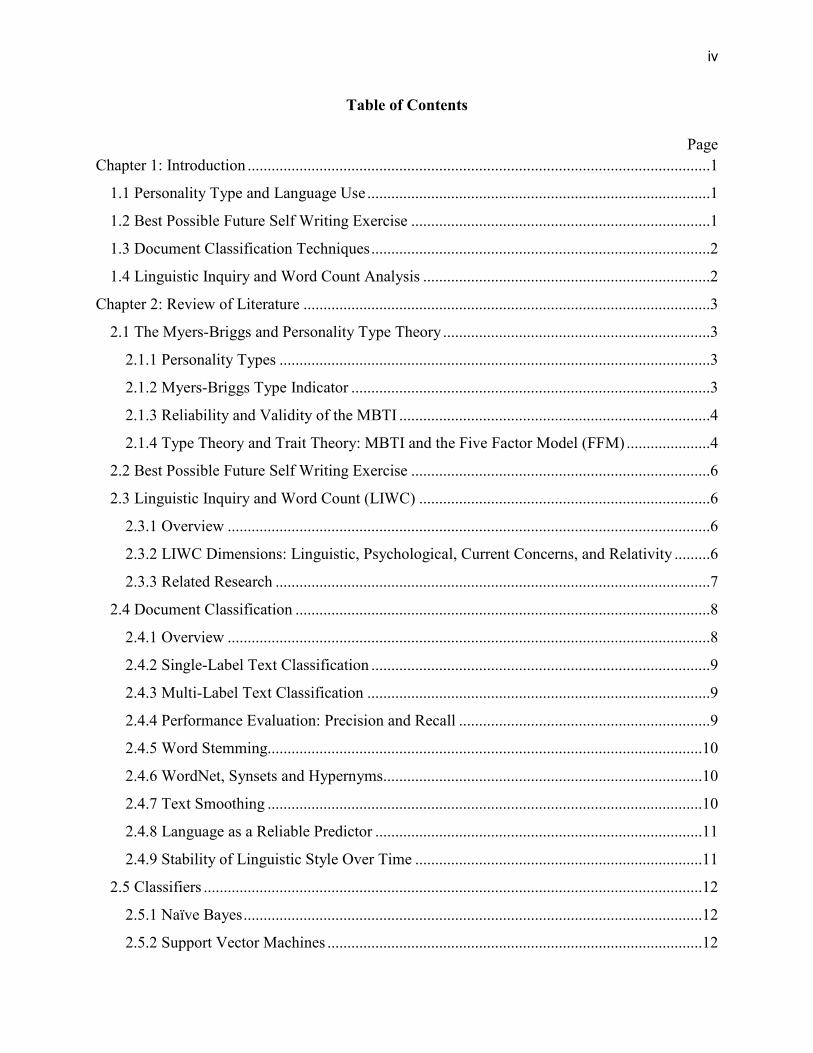
Table of Contents
Page
Chapter 1: Introduction ....................................................................................................................1
1.1 Personality Type and Language Use ......................................................................................1
1.2 Best Possible Future Self Writing Exercise ...........................................................................1
1.3 Document Classification Techniques .....................................................................................2
1.4 Linguistic Inquiry and Word Count Analysis ........................................................................2
Chapter 2: Review of Literature ......................................................................................................3
2.1 The Myers-Briggs and Personality Type Theory ...................................................................3
2.1.1 Personality Types ............................................................................................................3
2.1.2 Myers-Briggs Type Indicator ..........................................................................................3
2.1.3 Reliability and Validity of the MBTI ..............................................................................4
2.1.4 Type Theory and Trait Theory: MBTI and the Five Factor Model (FFM) .....................4
2.2 Best Possible Future Self Writing Exercise ...........................................................................6
2.3 Linguistic Inquiry and Word Count (LIWC) .........................................................................6
2.3.1 Overview .........................................................................................................................6
2.3.2 LIWC Dimensions: Linguistic, Psychological, Current Concerns, and Relativity .........6
2.3.3 Related Research .............................................................................................................7
2.4 Document Classification ........................................................................................................8
2.4.1 Overview .........................................................................................................................8
2.4.2 Single-Label Text Classification .....................................................................................9
2.4.3 Multi-Label Text Classification ......................................................................................9
2.4.4 Performance Evaluation: Precision and Recall ...............................................................9
2.4.5 Word Stemming.............................................................................................................10
2.4.6 WordNet, Synsets and Hypernyms................................................................................10
2.4.7 Text Smoothing .............................................................................................................10
2.4.8 Language as a Reliable Predictor ..................................................................................11
2.4.9 Stability of Linguistic Style Over Time ........................................................................11
2.5 Classifiers .............................................................................................................................12
2.5.1 Naïve Bayes ...................................................................................................................12
2.5.2 Support Vector Machines ..............................................................................................12

v
Chapter 3: Methodology .............................................................................................................13
3.1 Overview ..........................................................................................................................13
3.2 Examining Personality Type Using Linguistic Inquiry and Word Count ........................13
3.3 Natural Language Toolkit .................................................................................................14
3.4 Single-Label Binary naïve Bayes Classifier .....................................................................14
3.5 Support Vector Machine Classification............................................................................16
3.6 Word Smoothing ..............................................................................................................18
3.7 Stop-word Filtering ..........................................................................................................20
3.7 Porter Stemming ...............................................................................................................20
Chapter 4: Experiment ...................................................................................................................21
4.1 Data Collection .....................................................................................................................21
4.2 Experimental Goals ..............................................................................................................21
4.3 Myers-Briggs Type Indicator Reports ..................................................................................22
4.4 Best Possible Future Self Writing Samples ..........................................................................22
4.5 Linguistic Inquiry and Word Count (LIWC) Analysis ........................................................24
4.6 Naïve Bayes Classification ...................................................................................................25
4.6.1 Probabilistic Word-based Features ................................................................................25
4.6.2 Probabilistic LIWC-based Features ...............................................................................27
4.7 Support Vector Machine Classification ...............................................................................28
4.7.1 SVM Word-based Features ...........................................................................................28
4.7.2 SVM LIWC-based Features ..........................................................................................28
4.7.3 Kernel Choice and Parameterization .............................................................................29
Chapter 5: Results and Discussion .................................................................................................32
5.1 Experimental Overview ........................................................................................................32
5.2 Naïve Bayes Classification ...................................................................................................32
5.2.1 Word-based Results .......................................................................................................32
5.2.2 LIWC-based Results ......................................................................................................33
5.3 Support Vector Machine Classification ...............................................................................34
5.3.1 Word-based Results .......................................................................................................34
5.3.2 LIWC-based Results ......................................................................................................34
5.4 Conclusions ..........................................................................................................................35

vi
5.5 Future Work .........................................................................................................................37
References ......................................................................................................................................38
Appendices .....................................................................................................................................42
A. Descriptions of the Personality Type Dichotomies ...............................................................42
B. Descriptions of the 16 Psychological Types ..........................................................................43
C. Sample Myers-Briggs Type Indicator Step II Report ............................................................44
D. Scores of Participants Using the MBTI Step II .....................................................................45
E. A Search for Optimal Values of C and Gamma Using LibSVM ...........................................46
F. Stop-word Corpus Used in Word-based Classification Trials ...............................................47
G. Proposed Fix for a Logic Error in the NLTK Python Module ..............................................48
H. Results of the Classification Decisions by Document ...........................................................49

vii
List of Tables
Table
Page
1 Correlations of Self-Reported NEO-PI Factors With MBTI Continuous
Scales in Men and Women ......................................................................................................5
2 Population and Sample Distributions by Personality Preference ..........................................23
3 Sample Distribution By Personality Type .............................................................................23
4 Text-based Features of BPFS Essays .....................................................................................24
5 LIWC-MBTI Product-moment Correlation Coefficient ........................................................25
6 Preliminary Tests for Word-based Feature Space Conducted on T-F ...................................26
7 Preliminary Tests for SVM Kernel Selection ........................................................................30
8 Preliminary Tests for Alternative Classifier Selection ..........................................................31
9 Scores of Participants Using the MBTI Step II .....................................................................45
10 NLTK English Stop-word Corpus .........................................................................................47
11 Results of Classification by Document for E-I ......................................................................49
12 Results of Classification by Document for S-N .....................................................................50
13 Results of Classification by Document for T-F .....................................................................51
14 Results of Classification by Document for J-P ......................................................................53
15 Results of Subgroup Classification by Document for E-I .....................................................54
16 Results of Subgroup Classification by Document for S-N ....................................................55
17 Results of Subgroup Classification by Document for T-F.....................................................56
18 Results of Subgroup Classification by Document for J-P .....................................................57

viii
List of Figures
Figure
1 Each bag-of-words contains token counts relative to each label,
Introversion or Extraversion ..................................................................................................15
2 Common kernel functions used in SVM classification and regression .................................18
3 Preliminary tests for word smoothing ....................................................................................27
4 Results of the leave-one-out cross validation using the naïve Bayes classifier .....................33
5 Results of the leave-one-out cross validation using the SVM classifier ................................35

Chapter 1. Introduction
1.1 Personality Type and Language Use
Katherine Briggs and Isabel Briggs-Myers developed a personality inventory which was
initially used as an aid in placing women into jobs to which they would be comfortable and
productive. Myers-Briggs theory is a successor to Carl Jung's work on attitudes and functions. In
addition to attitude, Extraversion-Introversion, the Myers-Briggs typology contains three
functional dichotomies: the Thinking-Feeling (T-F) dichotomy describes whether someone is
logical in their judgments, or whether they base their decisions in personal or social values.
Judging-Perceiving (J-P) describes how an individual reveals themselves to the outside world. If
an individual prefers Judgment, then they will reveal their Thinking or Feeling nature. If they
prefer Perception, then they will exhibit outwardly those characteristics attributed to Sensing or
Intuition. Sensing-Intuition (S-N) reflects the two ways in which people are Perceiving--a
Sensing type will rely on the 5 senses and concrete observation while an Intuitive type will draw
upon conceptual relationships or possibilities when gathering information. Lastly, what Jung
referred to as attitude, Extraversion-Introversion (E-I), deals with how a person focuses their
energy and attention—whether outwardly focusing their perception or judgment on other people
or inwardly focusing upon concepts and ideas, respectively. Myers and Briggs work outlines 16
unique personality types using different combinations of the four bipolar continuums, or
dichotomies (Center for Applications of Psychological Type [CAPT], 2010).
The Myers-Briggs Type Indicator (MBTI) is the most widely used personality assessment
tool in the world. According to Myers (1998), an individual has a natural preference in each
dichotomy. The notion of type dominance within the four dichotomies is analogized to left or
right-handedness such that an individual maintains preferred ways of gathering data, analyzing it,
and responding. Preference entails that one prefers a single way of functioning, or a single
attitude, over the other, although an individual may still utilize their less dominant traits (Myers,
1998). Additionally, empirical evidence supports this notion of bipolarity of personality
preference (Tzeng et al., 1989).
Many personality assessment tools exist as forced-choice questionnaires. Pennebaker and
King (1999) argue that such a form of classification is ultimately limited by its design, and,
further, that an individual’s writing contains a greater depth of psychological meaning than could
be obtained from forced-choice questions.
1.2 Best Possible Future Self Writing Exercise
The Best Possible Future Self (BPFS) exercise was developed by psychologist Dr. Laura
King of Southern Methodist University. It was presented in The Health Benefits of Writing about
Life Goals (King, 2001) in which King asks participants to imagine and describe their future as if
everything went as well as it possibly could. This exercise was chosen for several reasons. First
of all, the BPFS contains elements of time, personal goals, self description, and rationale—it was
felt that it would provide a rich set of personal and stylistic attributes with which to differentiate
each unique personality preference. Secondly, the essay was already utilized as part of a course
on conflict management in which students took the Myers-Briggs Type Indicator. Lastly, there
are positive emotional and physical benefits associated with the exercise and expressive writing
in general, as documented by King (2001). For these reasons, it was felt that the BPFS essay was
an excellent candidate for the experiment. Next, I will describe document classification
techniques which will be applied to the sample data for essay classification into personality type
as well as supporting methods for textual analysis.
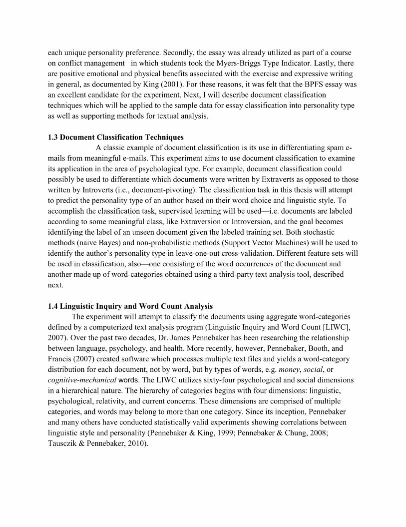
1.3 Document Classification Techniques
A classic example of document classification is its use in differentiating spam e-
mails from meaningful e-mails. This experiment aims to use document classification to examine
its application in the area of psychological type. For example, document classification could
possibly be used to differentiate which documents were written by Extraverts as opposed to those
written by Introverts (i.e., document-pivoting). The classification task in this thesis will attempt
to predict the personality type of an author based on their word choice and linguistic style. To
accomplish the classification task, supervised learning will be used—i.e. documents are labeled
according to some meaningful class, like Extraversion or Introversion, and the goal becomes
identifying the label of an unseen document given the labeled training set. Both stochastic
methods (naive Bayes) and non-probabilistic methods (Support Vector Machines) will be used to
identify the author’s personality type in leave-one-out cross-validation. Different feature sets will
be used in classification, also—one consisting of the word occurrences of the document and
another made up of word-categories obtained using a third-party text analysis tool, described
next.
1.4 Linguistic Inquiry and Word Count Analysis
The experiment will attempt to classify the documents using aggregate word-categories
defined by a computerized text analysis program (Linguistic Inquiry and Word Count [LIWC],
2007). Over the past two decades, Dr. James Pennebaker has been researching the relationship
between language, psychology, and health. More recently, however, Pennebaker, Booth, and
Francis (2007) created software which processes multiple text files and yields a word-category
distribution for each document, not by word, but by types of words, e.g. money, social, or
cognitive-mechanical words. The LIWC utilizes sixty-four psychological and social dimensions
in a hierarchical nature. The hierarchy of categories begins with four dimensions: linguistic,
psychological, relativity, and current concerns. These dimensions are comprised of multiple
categories, and words may belong to more than one category. Since its inception, Pennebaker
and many others have conducted statistically valid experiments showing correlations between
linguistic style and personality (Pennebaker & King, 1999; Pennebaker & Chung, 2008;
Tausczik & Pennebaker, 2010).

3
Chapter 2. Review of Literature
2.1 The Myers-Briggs and Personality Type Theory
2.1.1 Personality Types.
Jungian typology is a cognitive theory which posits that people use different mental
processes for taking information into their awareness and for making decisions. The Myers-
Briggs Type Indicator (MBTI) measures personality type on 4 dichotomies: Extraversion-
Introversion, Sensing-Intuition, Thinking-Feeling, and Judging-Perceiving (Myers, 1998). Each
dichotomy is a bipolar continuum, meaning that Thinking and Feeling are opposite sides of the
same scale. When a single component from each dichotomy is combined, they make up the full
psychological type of an individual—for example, the psychological type ESTJ stands for
Extraversion, Sensing, Thinking, Judging. Although Myers-Briggs theory dictates that one can
use both preferences in any dichotomy (though not at the same time since it would be
contradictory), it also states that people generally do not change preferences throughout their
lifetime. Appendix A shows the descriptions of the four dichotomies included in the MBTI
manual (Myers, 1998).
The following descriptions of the 4 dichotomies are summarized from CAPT (2010). The
Thinking-Feeling dichotomy describes whether someone is logical in their judgments, or whether
they base their decisions in personal or social values. Judging-Perceiving describes how an
individual reveals themselves to the outside world. If an individual prefers Judgment, then they
will reveal their Thinking or Feeling nature. If they prefer Perception, then they will exhibit
outwardly those characteristics attributed to Sensing or Intuition. S-N reflects the two ways in
which people are Perceiving--a Sensing type will rely on the 5 senses and concrete observation
while an Intuitive type will draw upon conceptual relationships or possibilities when gathering
information. Lastly, there is E-I, what Jung referred to as attitude, Extraversion-Introversion,
which deals with how a person focuses their energy and attention, whether outwardly focusing
their perception or judgment on other people or inwardly focusing upon concepts and ideas,
respectively (CAPT, 2010). Appendix B shows all 16 personality types, represented by letter
combinations of the four dichotomies, shown alongside standard descriptions associated with
each of the personalities as described in the MBTI manual (1998).
2.1.2 Myers-Briggs Type Indicator.
The MBTI is a forced-choice questionnaire in which a person selects the answer that best
fits their usual behavior. Because there is only a finite set of answers to choice from, this method
of questioning is called forced-choice, but it is also acceptable to not answer questions. The
MBTI assessment has been revised several times since its inception in 1942 by Isabelle Briggs-
Myers and Katherine Briggs, and is one of the most widely used psychological tools to date.
The detailed MBTI reports include a clarity index for each of an individual preference.
The scale of these clarity scores range from 0 to 30; however, the scores, themselves, do not
measure how much aptitude an individual has regarding their personality preference. Rather, the

4
clarity scores reflect the consistency of an individual to convey a given preference within the
questionnaire (Myers, 1998). Thus, a low score means that the assessment is less clear, and a
high score denotes that the questionnaire is very clear for a given preference, according to the
questionnaire. For a sample MBTI Step II report, please refer to Appendix C.
Individuals, after taking the assessment, receive detailed feedback in their report as well
as the opportunity to partake in what is referred to as the best-fit exercise with the administrator
of the assessment to either confirm or call into question the results of the report. A number of
studies have examined the validity of the Best-Fit Type, or Verified Type. According to
Schaubhut et al. (2009), a total of 8,836 individuals engaged in the MBTI Step I assessment as
well as the best-fit exercise, afterwards; 72.9% reported the same preferences as their report,
18.2% reported 3 out of 4 preferences to be correct, 6.9% reported correct on 2 preferences,
1.9% correct on 1 preference, and 0.1% said they were in disagreement with their reported types.
2.1.3 Reliability and Validity of the MBTI.
There is supporting evidence that the MBTI has favorable construct validity, internal
consistency, and test-retest reliability (Schaubhut et al., 2009). The step I MBTI has been shown
to meet or exceed the internal consistency and test-retest reliability when compared with other
well-known personality assessments according to research highlighted in the MBTI form M
manual supplement (Schaubhut et al., 2009). Data shows an internal consistency reliability of
0.90 or greater for the step I Myers-Briggs Type Indicator. In another study, the MBTI is shown
to correlate with 4 of the 5 factors with another widely used personality tool, the Five Factor
Model (McRae & Costa, 1989). Lastly, Tzeng et al. (1989) show significant empirical evidence
in support of the bipolarity of the preference dichotomies and in support of Myers-Briggs scores
being predictive of occupational preferences.
Because the data in this study contains writing samples from a diverse group of students,
there is a concern over subjects that learned English as a second language (ESL students). A
study at Montclair State University administered the Myers-Briggs Type Indicator to 74 ESL
students whose first language was Spanish (Call & Sotillo, 2010). Their data provides
correlations between Myers-Briggs scores and Group Embedded Figures Test (GEFT) scores,
which measures the cognitive variable of field sensitivity, and compares the results of the
independent group (the Spanish speaking group) with the results of MBTI and GEFT
correlations with students whose first language was English. The experiment provides evidence
in support of the MBTI as a statistically sound method for measuring personality types regardless
of first-language, at least with respect to the multi-national Spanish-speaking group.
2.1.4 Type Theory and Trait Theory: MBTI and the Five Factor Model (FFM).
Personality type theory looks at personality from the perspective of type dominance and
bipolarity. Trait theory, however, constructs its model based on the degree to which one
measures in a single trait. In the case of the Five Factor Model (or Big Five), these traits are
Extraversion (E), Agreeableness (A), Conscientiousness (C), Neuroticism (N), and Openness
5
(O). This study references the Five Factor Model because it is used by many researchers of
personality theory as well as by recent studies regarding personality type and language
(Pennebaker & King, 1999; Pennebaker & Chung, 2008). Supporting evidence shows the Myers-
Briggs Type Indicator to correlate with four of the Big Five traits (Furnham, 1996; McRae and
Costa, 1989).
The origins of the Five Factor model trace back to two researchers, Allport and Odbert,
who created a list of 17,953 traits that marked individual difference among people. The list they
created was subsequently shortened by British-American psychologist Raymond Cattell. Cattell's
12-dimensional model has been extensively reviewed, resulting in today's Five Factor Model.
The relevance of this model is considered an effect of its basis in natural language. The Five
Factor Model continues to show its effectiveness as a personality assessment tool. Although this
study does not use the Five Factor Model, some of the research drawn upon offers valuable
insight into linguistic style in terms of the Big Five.
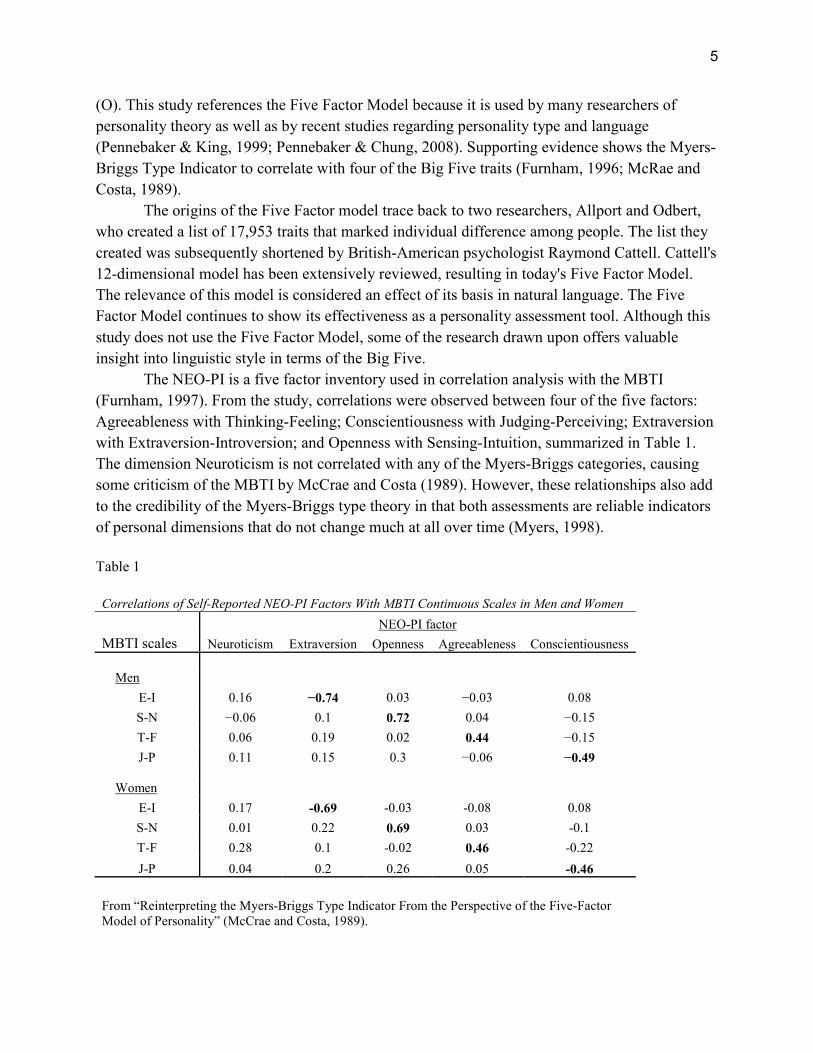
The NEO-PI is a five factor inventory used in correlation analysis with the MBTI
(Furnham, 1997). From the study, correlations were observed between four of the five factors:
Agreeableness with Thinking-Feeling; Conscientiousness with Judging-Perceiving; Extraversion
with Extraversion-Introversion; and Openness with Sensing-Intuition, summarized in Table 1.
The dimension Neuroticism is not correlated with any of the Myers-Briggs categories, causing
some criticism of the MBTI by McCrae and Costa (1989). However, these relationships also add
to the credibility of the Myers-Briggs type theory in that both assessments are reliable indicators
of personal dimensions that do not change much at all over time (Myers, 1998).
Table 1
Correlations of Self-Reported NEO-PI Factors With MBTI Continuous Scales in Men and Women
NEO-PI factor
MBTI scales Neuroticism Extraversion Openness Agreeableness Conscientiousness
Men
E-I 0.16 −0.74 0.03 −0.03 0.08
S-N −0.06 0.1 0.72 0.04 −0.15
T-F 0.06 0.19 0.02 0.44 −0.15
J-P 0.11 0.15 0.3 −0.06 −0.49
Women
E-I 0.17 -0.69 -0.03 -0.08 0.08
S-N 0.01 0.22 0.69 0.03 -0.1
T-F 0.28 0.1 -0.02 0.46 -0.22
J-P 0.04 0.2 0.26 0.05 -0.46
From “Reinterpreting the Myers-Briggs Type Indicator From the Perspective of the Five-Factor
Model of Personality” (McCrae and Costa, 1989).

6
2.2 Best Possible Future Self Writing Exercise
The Best Possible Self essay contains elements of self-description, at least two temporal
frames of reference, present time and in the future, as well as various contexts (e.g. work,
school, family, finances) with which authors of different personality types might reveal
themselves via word choice. Additional appeal for its use in human subject research is provided
by King (2001) which shows that writing about one's best possible self can actually be beneficial
to one's health.
King’s (2001) BPFS exercise is as follows:
Think about your life in the future. Imagine that everything
has gone as well as it possibly could. You have
worked hard and succeeded at accomplishing all of your
life goals. Think of this as the realization of all of your life
dreams. Now, write about what you imagined (p. 801).
2.3 Linguistic Inquiry and Word Count (LIWC)
2.3.1 Overview.
The Linguistic Inquiry and Word Count (LIWC) is a text analysis tool that differentiates
documents according to broad themes expressed in writing: psychological, relativity, and
contextual themes. LIWC was created by Dr. James Pennebaker in order to examine
relationships between language and personality. In an early study, Pennebaker and King (1999)
produced four reliable factors by differentiating linguistic traits in undergraduate students
enrolled in a psychological statistics course. Their study uses data collected over a number of
years. The four factors were labeled as Immediacy, Making Distinctions, Social Past, and
Rationalization. These labels were heavily influenced by the classical interpretations of motive in
psychology. In a study by Pennebaker and King (1999), the LIWC factors correlate with Five
Factor scores in a statistically significant study from a sample of 469 students. Tausczik and
Pennebaker (2010) discuss the development of the Linguistic Inquiry and Word Count (LIWC)
and its social and psychological dimensions in terms of attentional focus, emotionality, social
relationships, thinking styles, and individual differences.
The LIWC text analysis tool measures word usage based on functional and emotional
dimensions, as well as fourteen other linguistic dimensions, e.g. articles, pronouns, and verbs.
Specially crafted word-categories are used to categorize words based on a list of regular
expressions, attributing word stems to categories of social, psychological and contextual
significance. The program records the percentage of words recognized in each document, and
displays what percentage of the words matched word stems to particular themes, like sex* to
sexual words, happ* to positive emotional words, or even words related to contextual categories,
such as religion and money.
2.3.2 LIWC Dimensions: Linguistic, Psychological, Current Concerns, and Relativity.

7
According to Pennebaker and King (1999), the LIWC utilizes sixty-four psychological
and social dimensions to categorize words into a hierarchical nature. The hierarchy of categories
begins with four dimensions: linguistic, psychological, relativity, and current concerns. These
dimensions are comprised of multiple categories, and words may aggregate to more than one
category (Pennebaker & King, 1999).
The Linguistic dimension is comprised of 14 linguistic categories including hard
categories like verbs, pronouns, and articles as well as document attributes like average words
per sentence and word count. A word may be considered a verb but also be categorized as one or
more of the other psychological categories. It is not the case, however, that a verb be classified as
another part of speech.
Psychological dimensions include cognitive, social, and emotional categories. In many of
the dimensions, categories may be comprised of subcategories, like in the case of negative
emotions containing the subcategories anger (e.g. abuse, agitate) and sadness (e.g. alone, agony).
The cognitive categories include words like absolute and almost, or word stems like accura* and
ambigu*. Social words include child, colleague, and contact, just to name a few. Overall, the
psychological dimension is very rich with self-descriptors, cognitive and mechanical aspects, and
action-oriented verbs like cried, cries, and crying.
The Current Concerns dimension aggregates words into contextually relevant categories
like occupation, leisure, money, metaphysical, and physical states, like eating or sleeping.
Although context may be useful in determining aspects of motive or discourse, when speaking of
his initial undertakings, Pennebaker says, "...it gradually became apparent that it was far more
important to see how people talked about a given topic rather than what they were talking
about”, regarding the derivation of psychological information from linguistic style and content
(Pennebaker, 2002, p. 8).
The Relativity dimension is the parent category for time, space and motion. Time
subcategories are based on verb tense. Space subcategories are comprised of prepositions (like
above, across, or beneath) as well as adjectives and other parts of speech that reference space or
location. The inclusive word-category (e.g. and, with, and include) and the exclusive category
(e.g. but, without, and exclude) are also within the broader scheme of relativity. Finally, the
motion category contains words like arrive and went. Because LIWC utilizes regular
expressions, many of the word entries in the categories are word stems. Example motion word
stems are action* and advanc*. To see example results from LIWC, refer to Appendix D.
2.3.3 Related Research.
Pennebaker and King (1999) examined stream-of-consciousness (SOC) writings in terms
of linguistic dimensions and personality trait. Their experiment shows statistically significant
correlation between the four linguistic dimensions and the Five Factor scores of the authors. The
four linguistic dimensions were derived by Pennebaker and King (1999) using principal
component analysis on the LIWC dimensions from 838 stream-of-consciousness (SOC) writing
samples. The four dimensions derived from the study were labeled: Immediacy, Making

8
Distinctions, The Social Past, and Rationalization. Making Distinctions, for example, is a
dimension comprised of four LIWC text categories: tentative (e.g. depends, guess, hopeful,
luck), exclusive (e.g. but, either, or), negation (e.g. can’t, hasn’t, neither, not), and inclusive (e.g.
and, with, both). Their work highlights correlations between the LIWC categories and the Five
Factor scores for individuals. For example, three categories in the Making Distinctions
dimension (tentative, exclusive, and negations) correlate negatively with Extraversion on the
Five Factor scores.
Pennebaker and Chung (2008) used the LIWC to analyze self-descriptive essays.
Through principle component analysis using varimax rotation, they were able to show that factor
analysis on adjectives in the essays produced 7 factors which they found to be psychologically
meaningful. Interestingly, some of the factors were unipolar and some exhibited bipolarity.
Factors included 7 broadly labeled categories: Social, Evaluation, Self-Acceptance, Negativity,
Fitting In, Psychological, Stability, and Maturity. The highest factor, Sociability, included self-
descriptive adjectives like quiet, shy, outgoing, reserved, comfortable, open, friendly, and
insecure. One interesting point is that participants that used words like shy, or quiet, were
actually more likely to show positive correlation with Extraversion in the Five Factor scores.
However, in their earlier essay (Pennebaker & Chung, 1999), the analysis of stream-of-
consciousness (SOC) writings suggested the statistically significant positive correlation between
the LIWC Social category and Extraversion. It is not known if words in self-descriptive essays
often correlate with semantically opposite psychological traits, but it could mean that the context
of the writings hold the key to this mystery.
In another study, a Korean version of the Linguistic Inquiry and Word Count was used to
analyze eighty stream-of-consciousness writings with respect to Myers-Briggs and the Five
Factor model (Lee et al., 2007). The Korean study supported the evidence presented by
Pennebaker and King (1999) that certain LIWC categories and the Five Factor scores show
significant correlation. It is important to note that KLIWC is a much less extensive version of
LIWC. However, Lee et al. (2007) introduce correlations between the KLIWC and Myers-Briggs
types, but the focus of the study is primarily on linguistic categories and does not provide a
means of comparison across the same 64 psychological and contextual dimensions as the English
LIWC.
2.4 Document Classification
2.4.1 Overview.
Document classification techniques have become ubiquitous in the past decade. Search
engines take advantage of these methods to produce relevant search results from billions of
indexed websites in response to a few simple keywords. With billions of spam, or junk, e-mail
messages sent every day, e-mail servers utilize document classification techniques to filter out
junk mail by training the classifier with a sample of known spam e-mails. Documents can be
classified by supervised or unsupervised machine learning techniques. Unsupervised text
classification describes a form of document clustering and the evaluation of similarities or

9
differences in some feature set for an unlabeled corpus of samples. This study approaches the
problem of identifying personality type through document classification techniques using a
labeled training set. Thus, it uses supervised learning methods to train the classifier and make a
binary decision on an unseen document. All of the supervised learning techniques in this study
will perform single-label binary text classification.
2.4.2 Single-Label Text Classification.
Single-label text classification is a function in which a document is only given a single
label. There may be many labels from which to choose, but a document can only belong to one
class. For single-label binary text classification, there exists a set of documents, D = ( d1, d2, …,
d|D| ), and a binary label, C = { 0, 1 }, and an unknown function Φ`: D x C → { true, false }
which is a transitive, symmetric, and reflexive bijection between documents and the label, C
(Sebastiani, 2001). A single-label binary text classifier, Φ: D x C → { 0, 1 }, is then just an
approximation of the unknown function, Φ`. The error of the approximation E( Φ, Φ`) can be
used to evaluate the performance of the classifier. However, precision and recall, discussed in
section 2.4.4, provide a more detailed synopsis.
2.4.3 Multi-Label Text Classification.
In multi-label classification, many labels may be attributed to a single document. For a
set of documents, D = ( d1, d2, …, d|D| ), there exists a set of classes C = { c0, c1, …, c|C| }, and the
unknown function one wishes to approximate is Φ: D x C → { 1, 0 }. If and only if all single-
label components of the multi-label classification are stochastically independent of one another,
then the multi-label classification can be treated as the sum of the component parts (Sebastiani,
2001). In other words, a multi-label classification can be made from independent single-label
classifications, in such a case. Otherwise, if the classes (or labels) are not stochastically
independent, then the dimensionality of the problem space cannot be reduced to single-label
classification. It is important to note here that the four MBTI dichotomies are not independent of
one another. Due to this study’s sample size of 40, it would be pointless to attempt classification
using all four letters as a single label. Thus, each dichotomy is treated as an independent class to
make it possible to classify documents using multi-label text classification given the small
sample set.
2.4.4 Performance Evaluation: Precision and Recall.
In document classification trials, precision and recall are commonly used estimates for
performance evaluation. Recall is the number of relevant documents retrieved divided by the
total number of relevant items in the collection, and precision is the number of relevant
documents retrieved divided by the total documents retrieved (Jurafsky and Martin, 2009). The
experiment uses both measures to explain classifier performance. Certainly, a precise method is
desirable—a classifier that makes a decision only if it is fairly certain. However, recall is also
important as one wants to identify as many relevant items in the collection (or class) as possible.

10
Recall and precision will be used to assess the effectiveness of each classification method
attempted in this work.
2.4.5 Word Stemming.
Word stemming is a simple way to reduce the feature set of a corpus, and, in doing so,
reduce the sparseness of the data set. The simplest methods of word stemming use rule-based
processes like dropping suffixes -e, -es, -ed, and -ing. In computer literature, the most commonly
used stemming algorithm is Porter stemming (Porter, 1980). It is a back-off approach to word
aggregation by their word stems, effectively stripping suffixes, e.g. indicative becomes indic.
Word stemming algorithms can also incorporate n-Grams as well as use parts-of-speech to
improve the quality of selection among the stemming rules. The Natural Language Toolkit (Bird
et al., 2011) provides an implementation of the Porter stemmer used for this study.
2.4.6 WordNet, Synsets and Hypernyms.
Although WordNet will not be used in this study, its usefulness in expanding word
features is worthy of inclusion in this review. WordNet is a lexical database which enjoys an
active community of developers and contributors, including grants from the NSF, ARDA,
DARPA, DTO, and REFLEX. WordNet offers many tools used to examine, extrapolate, or
aggregate texts. Synonym-sets (synsets) are words which are equivalent in terms of information
retrieval (IR). WordNet includes the ability to generate these synsets for many common words.
WordNet can also find related nouns for a given adjective and the derivation of hypernyms.
Direct hypernyms are viewed as the thematic parent of a given verb. For example, bark, as in
“He barked out an order”, has direct hypernyms: talk, speak, mouth, verbalize, and utter.
WordNet can associate words with their inherited hypernyms, or parent themes. Sister terms are
other words that share the same parent. Thus, bark (in the sense of shouting), has sister terms
such as mumble, yack, rant, snap, sing, etc. Hyponyms are words that are a direct descendant of
another, and are also accessible for through WordNet for many nouns. One example of a
hyponym of canine would be dog, since all dogs are canines. WordNet can be used to get
definitions of words as well as direct hypernyms, inherited hypernyms, and sister terms. Each
feature of WordNet is based on its massive lexical database of 155,287 words organized into a
total of 117,659 synsets and have been created in dozens of other languages (Miller et al., 2010).
2.4.7 Text Smoothing.
In practice, when the chance of encountering an unknown word in a test corpus is high,
then classifiers in the domain of speech and language processing can benefit from the application
of data smoothing techniques. Smoothing techniques account for previously unseen attributes
and discount, or reduce, noise within the data set (Chen & Goodman, 1999).
There are a myriad of smoothing techniques that can account for zero-frequency events
(i.e., previously unseen words or tokens) in a word frequency distribution derived from an
arbitrary corpus. Examples of smoothing include Laplace (add-one) smoothing, Good-Turing

11
discounting, Witten-Bell smoothing, and Lidstone (additive) smoothing. Many of these
techniques are implemented through backoff. Backoff is a technique for using as many attributes
as possible while backing off those attributes if the feature space does not provide an example
with those exact features. In other words, if adequate data is not available, then use the next
largest attribute list that is found in the data set. In this manner, backoff is well-suited to work
with n-grams and other context-identity functions (Jurafsky & Martin, 2009).
2.4.8 Language as a Reliable Predictor.
The English language has been subject to change and revision in the past. The fluid
association of words and meanings allow phrases and words to be regularly created, abandoned,
or given new meanings through a host of psychological and sociological variables. For any
experiment relying on linguistic style and word choice, one must consider socially-based
phenomenon and generational changes in grammar, word selection, and word sense. Dr. George
Boeree studies how English moved from its Indo-European roots, with many complex and
irregular verb conjugations and many forms of noun declension (plurality, singularity,
possession, and gender), to the highly isolated language that it is today (Boeree, 2004).
Boeree (2004) concluded that the English language has undergone many sound changes
and includes borrowings from many other languages. However, Dr. Boeree also notes that
English has had very few spelling updates since the time of Shakespeare! So although
generational changes might exist, there are certainly many things that stay the same. To provide
a stable basis for research, one is inclined to use documents from the same time and location, and
in the same language. Soboroff et al. (1997) examine the utility of an unsupervised word-based
approach (using n-grams) to identify chapters by authorship; they show that linguistic style is
more important than language itself in classifying texts by author.
2.4.9 Stability of Linguistic Style over Time.
An important aspect of document authorship is whether or not the linguistic styles of an
author are consistent over long periods of time. Pennebaker and King (1999) show that linguistic
dimensions are reliable over time using a large body of text. Furthermore, they show that
variation of LIWC category-usage, e.g. negative and positive emotions, articles, and social
words, are tremendously impacted by the assigned topic. In another study, Mehl and Pennebaker
(2003) recorded conversations using an unobtrusive electronic recording device for 2-days at a
time and 4-weeks apart. The results of that study show that spontaneous word-usage of students
over a 4-week period did remain fairly consistent in the 16 dimensions regarded as reliable
measures of linguistic style by Pennebaker and King (1999) as well as seven other LIWC
categories thought to be applicable.
Personal pronoun use may provide information about people’s relative social networks
(Mehl & Pennebaker, 2003) as well as an indication of depression (Rude et al., 2004). One study
shows that first person plural pronoun use can actually increase in connection with an
emotionally charged event like the September 11 events (Chung & Pennebaker, 2007). The latter

12
research shows that the use of such function words is a reflection of the author’s cognitive
architecture (cognitive-reflection model) and that inducing people to use such words (as in a
Whorfian causal model) will not change their underlying cognitive architecture (Chung &
Pennebaker, 2007).
2.5 Classifiers
2.5.1 Naïve Bayes.
Naïve Bayes is a probabilistic method for classification which relies entirely on simple
observation (e.g. the probability of a word given some arbitrary class-label) and the assumption
that these observations are independent of one another (Heckerman, 1995). These classifiers rely
on an input space which, in text-based classification, is usually a bag-of-words—a class-based
distribution of word frequencies determined from a training set. From this training space, one is
able to classify unseen documents by determining which class from the training set is the likely
class to which the document belongs.
Naïve Bayes implementations are often used because they are simple and provide a
generalized decision. Naïve Bayes accounts for prior probabilities of a class when attempting to
make a classification decision. It uses what is referred to as the maximum a priori (MAP)
decision rule to classify unseen texts using the word frequencies for each class’s bag-of-words.
Naïve Bayes can even handle single-label multinomial decisions given adequate data. Naïve
Bayes and the MAP decision rule are described in the methodology section.
2.5.2 Support Vector Machines.
Support Vector Machines have their roots in binary linear classifiers. Geometrically-
based, they transform data into a higher-dimensional space using a kernel function, then, use a
separating hyperplane to make a decision boundary. The decision boundary allows for previously
unseen samples to be classified based on the hyperplane which separates attributes according to
their associated training labels (Cortes & Vapnik, 1995).
The hyperplane is measured by its functional margins, i.e. the distance between the
hyperplane and its closest training points. Support Vector Machines (SVMs) can use a linear or
non-linear kernel function—the difference being the transformation of the space in which the
optimal hyperplane is tried. SVMs can also include the use of slack variables. Slack variables
allow misclassified data points to be deemed acceptable losses according to a user-specified
threshold. Thus, even if the transformed input space is not linearly separable, an SVM using
slack variables can still correctly classify the observed data (Tristan, 2009). This classifier is
further described in the section on methodology.

13
Chapter 3: Methodology
3.1 Overview
In this experiment, the set of documents, D, is a set of responses to the open-ended
question, the Best Possible Future Self (BPFS) exercise presented by King (2001), each
document written by a unique author. The BFPS asks subjects to imagine and describe their
future as if everything went as well as it possibly could. Since the essays were written by student
participants, in class, the documents must be transcribed by hand.
This study will evaluate one stochastic classifier (naive Bayes) and one non-linear
classifier (Support Vector Machines) using leave-one-out cross-validation. Each feature set will
be a word-based input to a single classifier; the goal is to identify the personality preference of
an individual. The observed personality type is determined by the MBTI Step II—a total of four
dichotomies. In other words, based on the clarity scores provided by the Myers-Briggs Type
Indicator and text provided in the essays, we will determine the personality type of a test subject
based on an inference model created using empirical evidence gathered from the text. The
classification decision is applied to a test document, thereafter.
The first feature set consists of the term frequencies of the training set text. The second
feature set consists of word-categories defined by the Linguistic Inquiry and Word Count
(LIWC) text analysis tool (Pennebaker et al., 2007). One can use the LIWC categories as feature
sets to both naïve Bayes and SVM classifiers just like the word-based features. From these
results, one can explore the utility of the word-category based approach in determining
personality preference. It is important to note the use of leave-one-out cross-validation because it
impacts the validity of the study in that each single-document classification is its own trial.
Therefore, in each trial, the size of the test set is a single document, and the trial is conducted 40
times, rotating the assignment of test set among sample documents. Leave-one-out training is an
unbiased method for model selection (Elisseeff & Pontil, 2003).
Finally, this study compares the unique combinations of classifiers and feature sets using
precision and recall to evaluate the performance of the leave-one-out cross-validation trials.
From these results, one can evaluate the utility of classifiers and feature sets for the classification
task of identifying personality preference in individuals based on their BPFS responses.
3.2 Examining Personality Type Using Linguistic Inquiry and Word Count
The experiment incorporates the use of the Linguistic Inquiry and Word Count Tool
(LIWC) developed and maintained by experts over a period of ten years (Pennebaker et al.,
2007). LIWC has been shown to reveal meaningful psychological information from texts
(Pennebaker & King, 1999; Pennebaker et al., 2003; Pennebaker & Chung, 2008). LIWC
measures sixty-four functional and emotional dimensions as well as fourteen linguistic
dimensions. A specialized look-up dictionary is used to categorize words based on a list of
regular expressions, attributing each distinct regular expression to one or more categories of
social, psychological, or contextual significance. LIWC records how many words were actually

14
recognized in each document, and displays what percentage of the words matched regular
expressions to particular themes.
This study will also use the results of the LIWC in a simple correlation with the
participants’ Myers-Briggs scores, similar to methods undertaken in previous studies
(Pennebaker & King 1999; Lee et al., 2007) to identify features that may be useful in future
classification trials of such text as related to the MBTI.
McCrae and Costa (1989) provide supporting evidence that the Myers-Briggs
dichotomies correlate to 4 of the 5 traits in the Five Factor Model (FFM). So although this
experiment uses the Myers-Briggs types of the participants, and the assessment tool used in
similar studies is the Big Five Inventory (Pennebaker & King, 1999; Pennebaker & Chung,
2008), one can still make comparisons with Pennebaker’s foundational work to gain further
insight into word choice, linguistic style, and personality type.
3.3 Natural Language Toolkit
NLTK is text-processing software for use in natural language classification problems.
The open-source software has an active community of contributors and many publications have
utilized NLTK for tasks such as part-of-speech tagging, word sense disambiguation, spam e-mail
classification, and many classical NLP problems (Bird et al., 2011). The software is used here for
its Porter stemming method, stop-word corpus, smoothing methods, and convenient data
structures such as frequency distributions.
During experimentation, problems with NLTK’s Witten-Bell and Lidstone smoothing
methods were encountered. In the case of Witten-Bell smoothing, the error was discovered and
fixed by several parties simultaneously, shown in Appendix G. The Lidstone smoothing error
was more difficult to find so it was decidedly easier to rewrite the Lidstone smoothing method
for the purposes of this study. I have not been able to ascertain, through testing, whether or not
the Lidstone smoothing method was fixed in the latest version of NLTK (2.0.1rc1), but the issue
has been brought to the NLTK team’s attention by several individuals.
3.4 Single-Label Binary Naïve Bayes Classifier
At the time of this study, NLTK does not offer leave-one-out cross-validation so its built-
in naïve Bayes classifier will not be utilized. Instead, the experiments in this study incorporate
the use of naive Bayes as it is described in several papers (Rish, 2001; McCallum & Nigam,
1998). The naïve Bayes model utilizes a joint probability word distribution with priors calculated
from the training set. In naive Bayes, a simple bag-of-words can be built by counting all of the
tokens in the training documents partitioned by each document’s distinct label, Y = {+1, -1}.
Next, for each bag-of-words associated with a specific label, Y = {+1, -1}, one multiplies the
logarithms of each of the conditional probabilities for each word in the test document. Figure 1
exemplifies the bag-of-words concept using independently and identically distributed (IID)
priors, Pr(+1) = 0.5 and Pr(-1) = 0.5, shown as Introversion vs. Extraversion, for which there
exists m and n known unique word types associated with the labels. Note that in the experiments,

15
each model uses conditional probabilities dependent upon the prior probabilities of the classes
derived from the training set. As in Figure 1, each MBTI dichotomy can thus be modeled as a
binary set of word-based probability distributions.
Figure 1. Each bag-of-words contains word frequencies for each label, Introversion or Extraversion
Bayesian inference determines the likelihood that a hypothesis is true given a set of
observations, F, modeled as posterior probabilities. Models include probability trees, in naive
Bayes, or directed acyclic graphs (DAGs), in Bayesian networks, which can be used in Bayesian
inference. In document classification, it is common practice to assume that the prior distribution
of the classes, Pr(C), is independently and identically distributed; however, empirical priors can
also help to normalize conditional probabilities, Pr( F | C), in a hierarchical dependency model or
when DAGs are used to model dependencies (Li, 2007). With a sufficiently large data set,
examining the distribution of prior and posterior probabilities, one can make a reasonable choice
on whether the use of priors is deemed appropriate. The prior probabilities of each class will be
determined by the training set labels.
Per the law of large numbers, then, sample size has an obvious impact on the results of
Bayesian inference. One expects that the distribution will become a closer approximation to
actual values as the sample size increases. However, the joint probability distribution is not a
complete systematic representation of word choice because words may be encountered in a test
set which have never been seen in the training set, i.e. the zero-frequency problem. Data
smoothing techniques account for terms in which a previously unseen word is encountered in the
test case. Because the sample set is not large in the experiments, the study uses leave-one-out
training to maximize the training data while providing an unbiased method for evaluating each
classifier relative to the others (Elisseeff & Pontil, 2003). Afterwards, simple estimators can be
used to evaluate each classifier’s performance, i.e. precision and recall.
The formula found in Speech and Language Processing: An Introduction to Natural
Language Processing, Speech Recognition, and Computational Linguistics (Jurafsky & Martin,
2009) describes the maximum a posteriori (MAP) decision rule that is used to make a decision
on which class an essay is most likely to belong. For some arbitrary label, s ε S, and a feature

vector, f ε F, which represents the probability of a word given its lab
of words appearing in the unseen document,
(Jurafsky and Martin, 2009). ŝ � ������
For each test document, the conditional probability that a word belongs to an arbitrary
class is calculated as the number of times the word appears given the label, s, divided by the total
number of words that appear in the
validation, this entails that each MAP decision is associated with a training set that contains all
documents except the test document
test document exactly once. Thus
label, s, the likelihood estimate is based on the logarithmic product of all conditional
probabilities in a set, Pr( f ε F | s ), which appear in
made per the maximum a posteriori (MAP) decision rule.
works in the same manner as a word
counts) must be calculated using the number of words in each document and their associated
word-category distribution. For example, if 10% of the words are
contains 100 words, then exactly 10 words are articles. Note that this artificially inflates the total
word counts for each document since the word
fallacy in order to appropriately model the LIWC categories as independent
3.5 Support Vector Machine Classification
The experiments incorporate the use of libSVM
classification and regression. The methods follow procedures
(1995) as well as by Fletcher (2009
is the linear SVM. The linear SVM can be described as a model that incl
and some data, X, where x X has D attributes. Each training point is
label, Y = {+1, -1} such that there exists
yi {+1, -1} (Fletcher, 2009). For a model where the data {x
simple 2-dimensional space, an SVM would use a
x2} to separate {y1, y2} (Cortes &
The SVM is ideal because it was concluded by Vapnik
dimensional feature space is bounded by ratio of the expectation value of the number of support
vectors to the number of training vectors; thus, for larger data sets, Vapnik sta
consider only the support vectors which define the margins, as they can adequately provide an
optimal hyperplane for the linear separation of data by lessening the dime
space, thereby reducing the number of dimens
performance gain especially for text
into the tens of thousands.
vector, f ε F, which represents the probability of a word given its label, s, where n is the number
of words appearing in the unseen document, the MAP decision rule is shown here
������ �� � � �� | � ���� � �1
, the conditional probability that a word belongs to an arbitrary
class is calculated as the number of times the word appears given the label, s, divided by the total
the training documents, labeled s ε S. For leave-one
validation, this entails that each MAP decision is associated with a training set that contains all
documents except the test document; also, each document in the entire sample set is used as the
Thus, for a set of conditional probabilities given an arbitrary class
label, s, the likelihood estimate is based on the logarithmic product of all conditional
probabilities in a set, Pr( f ε F | s ), which appear in the unseen test case such that classification is
um a posteriori (MAP) decision rule. Using LIWC’s category
works in the same manner as a word-based model except that the term occurrences (the word
counts) must be calculated using the number of words in each document and their associated
category distribution. For example, if 10% of the words are articles in a document which
contains 100 words, then exactly 10 words are articles. Note that this artificially inflates the total
word counts for each document since the word-categories in LIWC overlap. One
fallacy in order to appropriately model the LIWC categories as independent dimensions
Support Vector Machine Classification
incorporate the use of libSVM, a library for Support Vector Machine
and regression. The methods follow procedures described by Cortes and Vapnik
2009). The simplest form of the Support Vector Machine (SVM)
is the linear SVM. The linear SVM can be described as a model that includes L training points
X has D attributes. Each training point is associated with a binary
1} such that there exists a feature space { xi, yi } for i = 1, 2, ..., L, x
For a model where the data {x1, x2} and two labels {y
dimensional space, an SVM would use a simple line or a continuous function on {x
& Vapnik, 1995).
he SVM is ideal because it was concluded by Vapnik (1982) that error in a high
dimensional feature space is bounded by ratio of the expectation value of the number of support
vectors to the number of training vectors; thus, for larger data sets, Vapnik states that
consider only the support vectors which define the margins, as they can adequately provide an
optimal hyperplane for the linear separation of data by lessening the dimensionality of the feature
space, thereby reducing the number of dimensions in the feature space. This results in a
performance gain especially for text-based classification tasks in which the features
16
el, s, where n is the number
is shown here in Equation 1
, the conditional probability that a word belongs to an arbitrary
class is calculated as the number of times the word appears given the label, s, divided by the total
one-out cross-
validation, this entails that each MAP decision is associated with a training set that contains all
; also, each document in the entire sample set is used as the
given an arbitrary class
label, s, the likelihood estimate is based on the logarithmic product of all conditional
unseen test case such that classification is
category-based model
based model except that the term occurrences (the word
counts) must be calculated using the number of words in each document and their associated
in a document which
contains 100 words, then exactly 10 words are articles. Note that this artificially inflates the total
One ignores this
dimensions.
library for Support Vector Machine
Cortes and Vapnik
. The simplest form of the Support Vector Machine (SVM)
udes L training points
associated with a binary
} for i = 1, 2, ..., L, xi RD, and
} and two labels {y1, y2} yield a
continuous function on {x1,
that error in a high-
dimensional feature space is bounded by ratio of the expectation value of the number of support
tes that one need
consider only the support vectors which define the margins, as they can adequately provide an
nsionality of the feature
feature space. This results in a
based classification tasks in which the features can number
In a multidimensional space where
can be described by w · xi + b = 0 where w (the normal to the hyperplane) and b are values used
to orient the hyperplane such that it is as far as possible from the nearest elements of y
planes, H1 and H2, are said to contain the points closest to the separating hyperplane. The points
that lie on these planes are the support vectors: w · x
The goal of the Support Vector Machine is to maximize the distance between the
hyperplane and the labeled sets of d
optimal hyperplane by maximizing
the margin, d2, the distance from H
from the support vectors such that
hyperplane that maximizes the distance between the training vectors, where the distance is
formulated from ���, � � min�: defined by the arguments (w0, b0
2009).
Cortes and Vapnik (1995)
1, 2, ..., L | xi RD and yi {+1,
b such that the following inequalities
� ∙ �" # � � ∙ �" # � $
The inequalities are valid for all data in the training set
can be reduced to a quadratic programming problem and can thus be solved for definite variables
in polynomial time as the optimal hyperplane can be written as a linear combination of training
vectors. This linear combination follows in equation 4.
�% � & '("��
It includes a set of Lagrange multipliers,
programming problem, )�Λ � Λ
where D is a symmetric L x L matrix such that D
If the data one wishes to classify is not fully separable, and
classification schema, Cortes and Vapnik
constrained, 0 $ +" $ , �-� . � 1strict the Support Vector Machine should be in determining whether or not the data is
sufficiently separable, or, rather, to what amount of slack we wish to allow misclassification
(Fletcher, 2009).
Additionally, SVMs include the ability to transform an input space based on a kernel
function. Such a function extends the feature space to a higher dimensionality by creating a
mapping from the input-space to a higher dimensional space using a non
In a multidimensional space where �" ∈ 01, the hyperplane that best separates the data
+ b = 0 where w (the normal to the hyperplane) and b are values used
to orient the hyperplane such that it is as far as possible from the nearest elements of y
contain the points closest to the separating hyperplane. The points
the support vectors: w · xi + b = +1 for H1 and w · xi + b =
The goal of the Support Vector Machine is to maximize the distance between the
labeled sets of data. Fletcher (2009) describes the problem of finding the
optimal hyperplane by maximizing the margins, d1, the distance from H1to the hyperplane, and
, the distance from H2 to the hyperplane to orient the hyperplane as far as possible
from the support vectors such that 2� � 23 � �||4|| (Fletcher, 2009). The optimal hyperplane is the
hyperplane that maximizes the distance between the training vectors, where the distance is
�� �∙4|4| 5 max�: �8� �∙4|4| such that the optimal hyperplane can be
0) that maximize the distance ���%, �% � 3|49| � Cortes and Vapnik (1995) show that a set of labeled training parameters, { x
{+1, -1}, are linearly separable if there exists a vector w and scalar
following inequalities, : 1 .� '" � 1 and (2) $ 1 .� '" � 51 (3) valid for all data in the training set (Cortes & Vapnik, 1995)
can be reduced to a quadratic programming problem and can thus be solved for definite variables
ime as the optimal hyperplane can be written as a linear combination of training
This linear combination follows in equation 4.
'" ∝"% �" �<=> ?>�? ∝"%: 0 �4
includes a set of Lagrange multipliers, Λ%A � BαC%, … , αC%E calculated from the quadratic ΛF 5 ΛFGΛ , and is subject to the constraints Λ :where D is a symmetric L x L matrix such that Dij = yi yj xi xj for i, j = 1, ..., L (Fletcher, 2009)
to classify is not fully separable, and one uses a binary
classification schema, Cortes and Vapnik (1995) show that the Lagrange multipliers1, … , H where C is the constraint parameter that describes how
Support Vector Machine should be in determining whether or not the data is
sufficiently separable, or, rather, to what amount of slack we wish to allow misclassification
Additionally, SVMs include the ability to transform an input space based on a kernel
function. Such a function extends the feature space to a higher dimensionality by creating a
space to a higher dimensional space using a non-linear function.
17
that best separates the data
+ b = 0 where w (the normal to the hyperplane) and b are values used
to orient the hyperplane such that it is as far as possible from the nearest elements of y Y. Two
contain the points closest to the separating hyperplane. The points
+ b = -1 for H2.
The goal of the Support Vector Machine is to maximize the distance between the
(2009) describes the problem of finding the
to the hyperplane, and
hyperplane as far as possible
The optimal hyperplane is the
hyperplane that maximizes the distance between the training vectors, where the distance is
such that the optimal hyperplane can be
3I49∙49 (Fletcher,
training parameters, { xi, yi } for i =
1}, are linearly separable if there exists a vector w and scalar
es & Vapnik, 1995). This problem
can be reduced to a quadratic programming problem and can thus be solved for definite variables
ime as the optimal hyperplane can be written as a linear combination of training
calculated from the quadratic : 0 �J2 ΛFK � 0
(Fletcher, 2009).
a binary
the Lagrange multipliers can be
where C is the constraint parameter that describes how
Support Vector Machine should be in determining whether or not the data is
sufficiently separable, or, rather, to what amount of slack we wish to allow misclassification
Additionally, SVMs include the ability to transform an input space based on a kernel
function. Such a function extends the feature space to a higher dimensionality by creating a
function.
18
Common non-linear kernels include polynomial, Radial Basis Function (RBF), and hyperbolic
tangent (tanh) kernels. These functions are shown in Figure 2, below. Once the input space is
transformed with one of the kernels, the SVM can handle non-linearly separable data.
Figure 2. Common kernel functions used in SVM classification and regression
The SVM classifier chosen was C-SVC due to its popularity in related works. As for the
parameter choice in C-SVC, the parameter C is called the constraint parameter and indicates how
strict the Support Vector Machine should be in determining whether or not the data is
sufficiently separable, or, rather, to what amount of slack one wishes to allow misclassification
(Fletcher, 2009). LibSVM uses the base-2 logarithm of C to compute the convergence tolerance
value. The parameter C is equivalent to nu, in nu-SVC, and either implementation is acceptable.
The second parameter, gamma, influences the smoothness of the decision boundary—a
high value for gamma can over-fit the training data, making it difficult for new, but dissimilar,
training points to be classified correctly. A very low value of gamma will generalize well but can
lead to under-fitting since the decision boundary will tend to have a much higher number of
support vectors (Fletcher, 2009).
As in the naïve Bayes approach, the experiments will utilize leave-one-out cross-
validation since it allows one to maximize the training data while providing an unbiased method
for evaluating the performance of different classifiers (Elisseeff & Pontil, 2003). The specific
forms of the kernels are documented in libSVM v3.1 (Bird et al., 2010). LibSVM provides a
simple interface with many kernel choices, advanced parameterization methods, and an interface
for the python language. For these reasons, it has become a widely popular tool for SVM
classification and regression, but many other free SVM libraries exist and work just as well.
3.6 Word Smoothing
The problem which smoothing solves can be described by a failure to account for every
word type in the unseen test set, known as the zero-frequency problem. Witten and Bell (1991)
describe four methods for smoothing in detail and analyze their ability to estimate the frequency
of a novel word based on a large corpus of text. Laplace smoothing is a generalization of
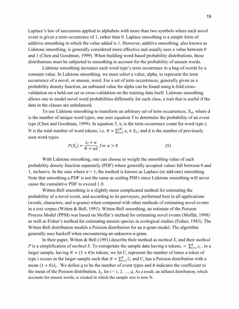
19
Laplace’s law of succession applied to alphabets with more than two symbols where each novel
event is given a term occurrence of 1, rather than 0. Laplace smoothing is a simple form of
additive smoothing in which the value added is 1. However, additive smoothing, also known as
Lidstone smoothing, is generally considered more effective and usually uses a value between 0
and 1 (Chen and Goodman, 1999). When building word-based probability distributions, these
distributions must be subjected to smoothing to account for the probability of unseen words.
Lidstone smoothing increases each word type’s term occurrence in a bag-of-words by a
constant value. In Lidstone smoothing, we must select a value, alpha, to represent the term
occurrence of a novel, or unseen, word. For a set of term occurrences, generally given as a
probability density function, an unbiased value for alpha can be found using k-fold cross-
validation on a held-out set or cross-validation on the training data itself. Lidstone smoothing
allows one to model novel word probabilities differently for each class, a trait that is useful if the
data in the classes are unbalanced.
To use Lidstone smoothing to transform an arbitrary set of term occurrences, Xd, where d
is the number of unique word types, one uses equation 5 to determine the probability of an event
type (Chen and Goodman, 1999). In equation 5, xi is the term occurrence count for word type i;
N is the total number of word tokens, i.e. L � ∑ �" ∈ NO|P|"�� ; and d is the number of previously
seen word types.
�N"̀ � �" # +L # +2 �-� + R 0 �5
With Lidstone smoothing, one can choose to weight the smoothing value of each
probability density function separately (PDF) where generally accepted values fall between 0 and
1, inclusive. In the case where α = 1, the method is known as Laplace (or add-one) smoothing.
Note that smoothing a PDF is not the same as scaling PDFs since Lidstone smoothing will never
cause the cumulative PDF to exceed 1.0.
Witten-Bell smoothing is a slightly more complicated method for estimating the
probability of a novel event, and according to its purveyors, performed best in all applications
(words, characters, and n-grams) when compared with other methods of estimating novel events
in a text corpus (Witten & Bell, 1991). Witten-Bell smoothing, an estimate of the Poisson
Process Model (PPM) was based on Moffat’s method for estimating novel events (Moffat, 1998)
as well as Fisher’s method for estimating unseen species in ecological studies (Fisher, 1943). The
Witten-Bell distribution models a Poisson distribution for an n-gram model. The algorithm
generally uses backoff when encountering an unknown n-gram.
In their paper, Witten & Bell (1991) describe their method as method X, and their method
P is a simplification of method X. To extrapolate the sample data having n tokens, � ∑ ="T"�� , to a
larger sample, having L � �1 # U J tokens, we let Ci represent the number of times a token of
type i occurs in the larger sample such that L � ∑ ,"T"�� and Ci has a Poisson distribution with a
mean �1 # U V" . We define q to be the number of event types and U indicates the coefficient to
the mean of the Poisson distribution, V", for i = 1, 2, …, q. As a result, an inflated distribution, which
accounts for unseen words, is created in which the sample size is now N.

20
Witten and Bell (1991) rest their analysis on the assumption that G(λ) is the empirical
cumulative distribution function for V�, … , VT . Given a sample of n tokens and q types of events
where ci is the number of occurrences of type i for 1 $ . $ W , the sample distribution is a Poisson
distribution with mean λi for i = 1, 2, …, q and a token count J � ∑ ="T"�� . This distribution is
transformed using Witten-Bell smoothing to estimate the Poisson distribution of a larger sample
set having L � ∑ ," � �1 # U JT"�� tokens. Thus, the probability of an event occurring k times is
calculated by ��X, V � YZ[\]^! (Weisstein, 2010), and the expected number of novel types in the
sample set is equivalent to Pr�J-bcd � W e c8Y B1 5 c8YfEg% 2h�V (Witten & Bell, 1991).
Witten and Bell found that estimating the probability of a novel event is equivalent to the
number of types that appear once divided by the size of the vocabulary, n. The model, then, for
estimating the probability of a novel event takes on the following form, ?� �� 5 ?3 ��i # ?j ��k 5 …
where each term, ti, represents the number of types that appear i times, divided by the vocabulary
n raised to a power of i. The actual probability following the Poisson process model is a
convergent series, and it is held that t1 / n is equivalent to the series in terms of performance.
3.7 Stop-word Filtering
Stop-words are words which generally act as syntactic sugar—for example, articles such
as the, a, or an give little insight into the content of a document but make the meaning of content
words more clear. A simple example of this concept could be the sentence: Birthday cake is a
family tradition. After stop-word filtering, it becomes Birthday cake family tradition. Stop-word
filtering has become commonplace in natural language processing, often improving the accuracy
of word-based classifiers by eliminating common words which offer less contextual meaning. An
English corpus of stop-words is included in the Natural Language Toolkit (Bird et al. 2010) and
also listed in Appendix F of this thesis. It can be argued that many of these stop-words do
provide contextual clues to the meaning of the text; however, the word-based classifiers in this
study do not use methods that take advantage of such clues.
3.8 Porter Stemming
The Porter stemming algorithm aims to remove suffixes from words, e.g. -y from happy.
To accomplish this task, Porter depicts all words as a series of one or more vowels as V and a
series of one or more consonants as C. In this way, he posits that all words take the form of
[C]VCVC…[V] where the brackets represent an optional series (Porter, 1980). The algorithm
uses a set of cardinal rules to remove the suffixes except where the word stem is kept under a
specific length. In his study, Porter (1980) demonstrates that a vocabulary of 10,000 words can
be reduced to 6,370 words based on his algorithm.

21
Chapter 4: Experiment
4.1 Data Collection
The data was collected over three semesters in 2010 and 2011 as part of a course on
conflict management offered to graduate students. Permission for the use of the data was
authorized by each participant via signature under the agreement that any marks of personal
identification such as gender, age, or names would be removed from the documents. Further,
participants were not compensated for their contributions in any way, and not all students chose
to participate in the study. Because the study involved human subjects’ personal thoughts and
confidential Myers-Briggs scores, approval from the Institutional Review Board (IRB) and full
consent of the participants was required before the data could be examined. Once the approval
for data collection was obtained from the IRB, IRB training was undertaken for the handling of
human subject data.
The data consists of two parts–the Myers-Briggs Type Indicator Step II (MBTI) results
and the Best Possible Future Self (BPFS) essays. In class, the BPFS exercise was given first, and
the MBTI assessments were given at a later date. The MBTI scores and essays were labeled with
non-identifying numbers, maintaining the relationship between BPFS essays and MBTI scores.
Both the Myers-Briggs assessment and BPFS exercise were provided as enrichment activities in
a course on conflict resolution. The essays were transcribed and digital scans of the MBTI
reports were sent (with identifying marks removed). In all, 40 participants contributed data.
Students also participated in self-validation of the MBTI scores under the guidance of a certified
practitioner.
4.2 Experimental Goals
In total, there are four personality type dichotomies: E-I, S-N, T-F, and J-P, where only
one preference in each dichotomy can be the dominant one. For classification purposes, one may
treat these dichotomies independently, thus, resulting in a decision for each one. Hence, each
document will be subject to four separate binary classification problems using leave-one-out
cross-validation.
Given the small sample size, one might consider leave-one-out cross-validation to
improve the results of the accuracy in a classification task. This method of cross-validation is a
useful approach to unbiased model selection (Elisseeff & Pontil, 2003). Since each classification
task is a binary decision for a single dichotomy, the resulting experiment is conducted over each
dichotomy. A training set of N-1 documents is built, leaving a single unseen document for
classification. Thus, there will be four independent classification trials (one for each dichotomy)
a total of N = 40 independent classification trials over each dichotomy. To evaluate the
performance of each classifier, the precision and recall are calculated over the entirety of the
leave-one-out trials for each dichotomy.
Similarities among the participants—education level, geographic location, and academic
interests—yield a narrower demographic, complicating the case for extending the results to the

22
general population, thereby hampering our ability to make bold statements about the
experiment’s translational validity. Although an assumption that personality type is a tractable
attribute for an individual, content validity is a challenge because language and personality types
are not tangible, or even necessarily quantifiable. All imperfect measures (personality assessment
tools, LIWC, smoothing techniques, and classifiers) may contribute to error and outcomes cannot
be attributed to any single device in this exploratory study. However, one cannot help but
attribute the successful implementation of such methods to a link between personality type and
word choice. For these reasons, one must be reminded of the exploratory nature of this study and
its sample size before forming conclusions.
Besides naïve Bayes and SVMs, other classifiers were considered for this study. Table 8
shows the trial runs for two such alternatives, a decision tree classifier and a linear regression
classifier, which both performed rather poorly and were eliminated from candidacy early on.
4.3 Myers-Briggs Type Indicator Reports
With respect to population data (Center for Application of Psychological Type [CAPT],
2010), the distribution of personality types in the sample group were fairly consistent with U.S.
estimated frequencies in Thinking-Feeling and Judging-Perceiving. Table 2 denotes the
frequencies of the sample MBTI scores compared with that of the general population. If one
looks at the first dichotomy pair (Introversion and Extraversion), then it is apparent that
Introverts are underrepresented in this study, though the other dichotomies are fairly balanced.
Forty students were given the MBTI Step II. After receiving their MBTI reports, the
students took part in self-validation of their scores (known as the Best Fit exercise). A table
containing the actual Myers-Briggs scores in the sample group can be found in Appendix D. Of
16 possible psychological types, 15 were represented in the sample of 40 students as shown in
Table 3. Of those types, 31.25% were singularly represented. The prediction of authors’ Myers-
Briggs scores may be impacted by the large number of Extraverts and small number of
Introverts. The large number of ENFPs, 7, enrolled in the course also stands out as unusual.
As mentioned earlier, clarity scores represent the confidence that the MBTI has in its
classification of a person’s preference. In response to a concern over clarity scores, it was
decided to conduct the experiments using two groups—the first of which uses leave-one-out
cross-validation over all samples while the second is a subset of the first, based on the MBTI
clarity scores of authors. The second group includes 75% of the original samples—authors who
had the highest clarity scores for their given preferences. In this way, one hopes to overcome
ambiguities related to preferences which are less clear. The two groups were created separately
for each preference, a total of 8 sample groups.
4.4 Best Possible Future Self Writing Samples
All participants were given the King’s (2001) Best Possible Future Self writing exercise
in a classroom setting and given twenty minutes to complete the assignment. It was apparent that
English was not the first language for every participant involved. The level of English fluency

23
has an unknown impact on the experiment. If such essays were to be removed, it could have a
large impact on the sample distribution given its already small size. However, labeling
documents from ESL (English as a Second Language) students would have made students easily
identifiable and so those factors were not recorded, in accordance with decisions made early on
through IRB approval.
Table 2
Population and Sample Distributions by Personality Preference
Personality Type
Est. Population
Distribution Sample Distribution
Extraversion 49.00% 65.00% (26)
Introversion 51.00% 35.00% (14)
Sensing 70.00% 52.50% (21)
Intuition 30.00% 47.50% (19)
Thinking 45.00% 47.50% (19)
Feeling 55.00% 52.50% (21)
Judging 58.00% 60.00% (24)
Perceiving 43.00% 40.00% (16)
Note. Population distributions reported in "Jung's Theory of Psychological Types
and the MBTI® Instrument", (CAPT 2010). In the sample distribution, N = 40
samples.
Table 3
Sample Distribution By Personality Type
ESTJ ESTP ESFJ ESFP ENTJ ENTP ENFJ ENFP
3 2 4 2 4 1 3 7
ISTJ ISTP ISFJ ISFP INTJ INTP INFJ INFP
5 2 3 0 1 1 1 1
Note. N = 40 samples.
The word counts in the sample set—unique word types, total tokens, average words-per-
document (WPD), average words-per-sentence (WPS), and average word types-per-document
(WTD)—are seen in Table 4, below, based on personality preference. Table 4 shows the data
before and after conducting Porter stemming and stop-word removal. The difference in the
number of unique word-types for Extraversion and Introversion suggests that many more
samples are needed to make a clear evaluation of the dichotomy E-I with respect to classification
methods. Judging-Perceiving may also suffer from this imbalance, and thus be subject to
complications introduced by an unbalanced data set, as well.

24
Table 4
Text-based Features of BPFS Essays___________________________________________ Before Porter stemming and stop-word filtering.
MBTI
Dichotomies
Sample
Distribution
Word
Types
Word
Tokens
Average
WPD
Average
WPS
Average
WTD
Extraversion 65% (26) 1859 10428 401.1 16.0 71.5
Introversion 35% (14) 1140 5275 376.8 16.9 81.4
Sensing 53% (21) 1455 7913 376.8 16.6 69.3
Intuition 48% (19) 1594 7790 410.0 16.1 83.9
Thinking 48% (19) 1348 6879 362.1 16.3 70.9
Feeling 53% (21) 1685 8824 420.2 16.3 80.2
Judging 60% (24) 1389 6210 388.1 16.4 86.8
Perceiving 40% (16) 1649 9493 395.5 16.3 68.7
After Porter stemming and stop-word filtering.
MBTI
Dichotomies
Sample
Distribution
Word
Types
Word
Tokens
Average
*WPD
Average
*WPS
Average
*WTD
Extraversion 65% (26) 1376 5631 216.6 8.7 52.9
Introversion 35% (14) 846 2834 202.4 9.1 60.4
Sensing 53% (21) 1067 4335 206.4 9.1 50.8
Intuition 48% (19) 1178 4130 217.4 8.5 62.0
Thinking 48% (19) 1015 3718 195.7 8.8 53.4
Feeling 53% (21) 1224 4747 226.0 8.8 58.3
Judging 60% (24) 1030 3312 207.0 8.7 64.4
Perceiving 40% (16) 1207 5153 214.7 8.8 50.3
Note. Population distribution was reported in "Jung's Theory of Psychological Types and the
MBTI® Instrument", (CAPT 2010). N = 40 sample documents.
4.5 Linguistic Inquiry and Word Count Analysis
The Linguistic Inquiry and Word Count program (Pennebaker et al., 2007) was used to
provide an alternative feature set to that of the entirely word-based feature sets. LIWC creates a
new feature set from an arbitrary document based on the categories to which words are
attributed. Additionally, words may belong to more than one category in LIWC.
Pearson’s product-moment correlation coefficient was calculated using the LIWC
category frequencies and MBTI clarity scores. Since each dichotomy is a single bipolar
dimension, a clarity score of 0 was supplied for the non-dominant preferences in the correlation.
The prominent correlations between LIWC and MBTI for the samples are shown in Table 5,

25
below. The correlation coefficient was calculated using the OpenStat Advanced Statistical
Package (Miller, 2010).
Table 5
LIWC-MBTI Product-moment Correlation Coefficient
LIWC word category E I S N T F J P
You 0.07 0.17 0.01 -0.07 0.04 -0.11 -0.24 0.35
They 0.11 -0.24 -0.34 0.37 0.03 0.10 -0.29 0.14
Past 0.12 0.09 0.14 -0.19 0.40 -0.17 0.04 -0.19
Adverb -0.03 0.16 -0.10 0.01 -0.10 -0.10 0.19 -0.31
Negation -0.27 0.36 0.02 -0.03 -0.22 0.06 0.21 -0.07
Number 0.00 0.03 0.16 -0.28 -0.17 -0.08 0.26 -0.13
Social 0.32 -0.27 -0.08 0.06 -0.07 0.07 -0.04 0.00
Anxiety -0.16 0.43 0.15 -0.04 -0.18 -0.11 0.08 -0.17
Sadness -0.12 0.37 0.34 0.04 -0.14 0.01 0.12 -0.14
Cognitive mechanical 0.07 0.09 -0.29 0.30 0.07 0.11 0.10 -0.04
Inhibition -0.13 0.47 0.15 0.04 -0.21 0.06 0.24 -0.01
See -0.15 0.08 -0.08 0.11 0.31 -0.14 -0.10 0.15
Feel 0.05 0.36 -0.07 0.10 -0.07 0.17 -0.02 0.07
Biology 0.00 0.02 -0.08 0.25 -0.31 0.29 0.07 -0.04
Body 0.14 -0.01 -0.21 0.54 -0.29 0.37 -0.14 0.23
Work -0.20 0.01 0.22 -0.49 0.01 -0.24 0.06 -0.16
Achieve -0.22 0.10 0.33 -0.32 -0.10 0.03 0.02 0.03
Motion 0.11 -0.32 -0.24 0.33 -0.28 -0.02 -0.31 0.28
Space -0.24 -0.04 -0.09 0.03 0.05 -0.18 -0.23 0.00
Non-fluencies -0.18 0.03 -0.11 -0.11 0.35 -0.39 0.04 -0.11
Question mark -0.24 0.02 -0.24 0.35 0.11 -0.09 -0.23 -0.09
Note. Of the 84 categories, the coefficients listed above were the most distinguished.
4.6 Naïve Bayes Classification
4.6.1 Probabilistic Word-based Features.
The naïve Bayes classifier utilizes a bag-of-words input space, i.e. a count of the token
occurrences for each given training set. Each preference is tested and represented using an
independent bag-of-words. For example, Extraversion and Introversion will be assigned
independent bags-of-words and be pitted against one another using the MAP decision rule. The
term occurrences of the training set data are used to calculate the conditional probabilities of the
word types, given their labeling. The distribution of prior probabilities (i.e. the probability that an
arbitrary document belongs to a given class) will be calculated from the training data, as well.
Since a smoothing method had not yet been decided upon, feature sets were tested using
Support Vector Machines since they are not subject to the zero-frequency problem. The
preliminary tests shown in Table 6 used nu-SVC within libSVM and an RBF kernel—its
parameters selected manually. The results in Table 6 give fairly similar results for all

26
dichotomies, regardless of the input features used. However, using Porter stemming and stop-
word filtering together produced the most well-balanced results so it was determined that further
trials using word-based feature sets would be subjected to both Porter stemming and stop-word
filtering. The preliminary results of table 6 used Laplace smoothing.
Table 6
Preliminary Tests for Word-based Feature Spaces with nu-SVC Stop-
word
filtering Stemming
No stemming
Unigram word vector
Unigram word vector
True T True F Precision
True T True F Precision
Pred. T 12 9 57.14%
Pred. T 10 6 62.50%
Pred. F 7 12 63.16%
Pred. F 9 15 62.50%
Recall 63.16% 57.14%
Recall 52.63% 71.43%
Accuracy 60.00%
Accuracy 62.50%
Bigram word vector
Bigram word vector
True T True F Precision
True T True F Precision
Pred. T 12 10 54.55%
Pred. T 12 9 57.14%
Pred. F 7 11 61.11%
Pred. F 7 12 63.16%
Recall 63.16% 52.38%
Recall 63.16% 57.14%
Accuracy 57.50%
Accuracy 60.00%
No
word-
filtering
Stemming
No stemming
Bigram word vector
Bigram word vector
True T True F Precision
True T True F Precision
Pred. T 12 10 54.55%
Pred. T 12 9 57.14%
Pred. F 7 11 61.11%
Pred. F 7 12 63.16%
Recall 63.16% 52.38%
Recall 63.16% 57.14%
Accuracy 57.50%
Accuracy 60.00%
The specific smoothing method for word-based classification was selected after
preliminary trials using several smoothing methods: Lidstone, Witten-Bell, and Good-Turing. To
determine the best method of data smoothing to be used with the word-based naïve Bayes
classifier, several smoothing methods were tested using leave-one-out cross validation over the
entire data set. Smoothing functions were carried out via the python interface to the Natural
Language Toolkit (Bird et al., 2010).
During Lidstone smoothing trials, a 2-dimensional range of alpha values were tried.
During Witten-Bell smoothing, the number of bins used was the ratio of types to tokens, as is

27
commonly done in practice. Consequently, Lidstone smoothing produced the best accuracy in
simple trials and so it was chosen for further trials using naïve Bayes. These preliminary results,
using the entire data set, are shown in Figure 3 below. To eliminate bias in the remaining trials,
all values for alpha are determined through leave-one-out cross-validation over the training set
only, and the unbiased values of alpha are used in Lidstone smoothing independently, for each
classification task during leave-one-out cross-validation over the entire sample set.
a. b.
c.
Figure 3. Preliminary tests for word smoothing
a.) Lidstone smoothing with an alpha value of 0.7 using N = 40 documents
b.) Witten-Bell smoothing, N = 40, using a novel event probability of |types| / |tokens|
c.) Good-Turing smoothing, N = 40
4.6.2 Probabilistic LIWC-based Features.
The LIWC word-categories will be tried in classification tasks separately from the word-
based features. Neither Porter stemming nor stop-word filtering is used in conjunction with
LIWC-based feature sets because the LIWC features are word-categories. To use the LIWC-
based features for naïve Bayes classification, one makes the necessary assumption that all word-
categories within LIWC are independent of one another. This entails that for each MBTI
I E S N T F P J
Prec. 0.19 0.00 0.90 0.85 1.00 0.70 0.67 0.68
Recall 0.43 0.00 0.86 0.89 0.53 1.00 0.38 0.88
0%
20%
40%
60%
80%
100%
Percentage
Word-based naive BayesLidstone Smoothing, N = 40
I E S N T F P J
Prec. 0.35 0.00 0.47 0.44 0.47 0.50 0.38 0.00
Recall 1.00 0.00 0.33 0.58 0.95 0.05 0.94 0.00
0%
20%
40%
60%
80%
100%
Percentage
Word-based naive BayesWitten-Bell Smoothing, N = 40
I E S N T F P J
Prec. 0.35 0.00 0.48 0.42 0.44 0.25 0.40 0.60
Recall 1.00 0.00 0.48 0.42 0.84 0.05 0.88 0.13
0%
20%
40%
60%
80%
100%
Percentage
Word-based naive Bayes Good-Turing Smoothing, N = 40

preference, e.g. Extraversion, a bag
based word occurrences for all docume
occurrences are easily calculated for an arbitrary word
occurrences (for a category and class) to the total number of words associated with all word
categories in that class. Although this falsely inflates the number of word tokens per class (
actual categories defined by LIWC are not mutually exclusive
is a simple way to model the LIWC
Since the zero-frequency issue is still relevant, but the
word-base term frequencies, one uses
experiment. With such densely populated
value between 0 and 1 would have little effect on the outcome
4.7 Support Vector Machine Classification
4.7.1 SVM Word-based Features
For the word-based SVM, stop
stop-word corpus and Porter stemming is applied to the remaining terms
is the set of conditional word probabilities, P(word
…, n such that L is the number of documents and n is the number of attributes (
stems) per document. It is important to note that each feature, word
independently of the other word features.
smallest value for all documents is assigned a value of 0,
document has the highest value for that attribute.
With SVMs, one is not required
simply dropped during scaling and
vectors themselves have a bearing on classification
preparation for the training and test data
applied to the training set, and its scaling factors used to normalize the word frequencies of the
test document; this is done for each independent trial of the leave
Figure 5, below, illustrates this process model.
4.7.2 SVM LIWC-based Features
It is important to reiterate that
conjunction with LIWC-based feature sets.
are given as word-category percent
arbitrary word-category. Thus, the features sets are
in the decimal range, [0, 1]. Data will be scaled in
feature set, using min-max normalization included as part of libSVM’s automated test scripts
(Chang & Lin, 2011). The total number
features. In all, 77 features are used from the LIWC progr
, a bag-of-words is constructed from the summation of
for all documents labeled with the preference letter, E. Such t
occurrences are easily calculated for an arbitrary word-category by the ratio of actual term
occurrences (for a category and class) to the total number of words associated with all word
t class. Although this falsely inflates the number of word tokens per class (
actual categories defined by LIWC are not mutually exclusive), the assumption of independence
a simple way to model the LIWC word-categories as a probability distribution.
frequency issue is still relevant, but the LIWC data not nearly
one uses Laplace (or add-one) smoothing to simplify the
. With such densely populated data given by LIWC, a different additive smoothing
have little effect on the outcome of the classifier.
Classification
based Features.
based SVM, stop-words are filtered from the text using the NLTK English
and Porter stemming is applied to the remaining terms. The feature set, x
is the set of conditional word probabilities, P(wordj | documenti) for i = 1, 2, …, L and j = 1, 2,
of documents and n is the number of attributes (total unique word
) per document. It is important to note that each feature, wordj for j = 1, 2, …, n, is scaled
independently of the other word features. An attribute of an arbitrary document having the
smallest value for all documents is assigned a value of 0, or, alternatively, a value of 1 if the
document has the highest value for that attribute.
required to address the zero-frequency problem. Z
simply dropped during scaling and have no bearing on the SVM classifier, as only the support
vectors themselves have a bearing on classification. Thus, scaling the data should be adequate
the training and test data prior to classification. Min-max normalization will be
training set, and its scaling factors used to normalize the word frequencies of the
t; this is done for each independent trial of the leave-one-out cross-validation.
llustrates this process model.
based Features.
It is important to reiterate that neither Porter stemming nor stop-word filtering is used in
based feature sets. For the LIWC-based SVM classifier, the feature sets
egory percentages—a percentage of words in the document
the features sets are the unaltered LIWC percentages represented
Data will be scaled in the same manner as the word-
max normalization included as part of libSVM’s automated test scripts
he total number of attributes will be significantly fewer than word
used from the LIWC program to generate the training and test
28
the summation of category-
Such term
category by the ratio of actual term
occurrences (for a category and class) to the total number of words associated with all word-
t class. Although this falsely inflates the number of word tokens per class (the
the assumption of independence
a probability distribution.
nearly as sparse as
to simplify the
LIWC, a different additive smoothing
text using the NLTK English
. The feature set, xi RD,
) for i = 1, 2, …, L and j = 1, 2,
total unique word
for j = 1, 2, …, n, is scaled
attribute of an arbitrary document having the
or, alternatively, a value of 1 if the
Zero counts are
, as only the support
caling the data should be adequate
ormalization will be
training set, and its scaling factors used to normalize the word frequencies of the
validation.
word filtering is used in
based SVM classifier, the feature sets
percentage of words in the document belong to an
the unaltered LIWC percentages represented
-based, SVM
max normalization included as part of libSVM’s automated test scripts
than word-based
am to generate the training and test
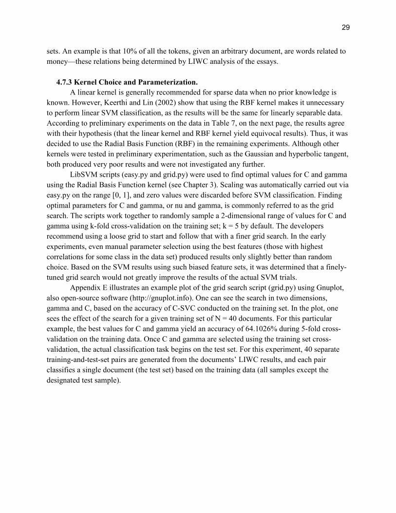
29
sets. An example is that 10% of all the tokens, given an arbitrary document, are words related to
money—these relations being determined by LIWC analysis of the essays.
4.7.3 Kernel Choice and Parameterization.
A linear kernel is generally recommended for sparse data when no prior knowledge is
known. However, Keerthi and Lin (2002) show that using the RBF kernel makes it unnecessary
to perform linear SVM classification, as the results will be the same for linearly separable data.
According to preliminary experiments on the data in Table 7, on the next page, the results agree
with their hypothesis (that the linear kernel and RBF kernel yield equivocal results). Thus, it was
decided to use the Radial Basis Function (RBF) in the remaining experiments. Although other
kernels were tested in preliminary experimentation, such as the Gaussian and hyperbolic tangent,
both produced very poor results and were not investigated any further.
LibSVM scripts (easy.py and grid.py) were used to find optimal values for C and gamma
using the Radial Basis Function kernel (see Chapter 3). Scaling was automatically carried out via
easy.py on the range [0, 1], and zero values were discarded before SVM classification. Finding
optimal parameters for C and gamma, or nu and gamma, is commonly referred to as the grid
search. The scripts work together to randomly sample a 2-dimensional range of values for C and
gamma using k-fold cross-validation on the training set; k = 5 by default. The developers
recommend using a loose grid to start and follow that with a finer grid search. In the early
experiments, even manual parameter selection using the best features (those with highest
correlations for some class in the data set) produced results only slightly better than random
choice. Based on the SVM results using such biased feature sets, it was determined that a finely-
tuned grid search would not greatly improve the results of the actual SVM trials.
Appendix E illustrates an example plot of the grid search script (grid.py) using Gnuplot,
also open-source software (http://gnuplot.info). One can see the search in two dimensions,
gamma and C, based on the accuracy of C-SVC conducted on the training set. In the plot, one
sees the effect of the search for a given training set of N = 40 documents. For this particular
example, the best values for C and gamma yield an accuracy of 64.1026% during 5-fold cross-
validation on the training data. Once C and gamma are selected using the training set cross-
validation, the actual classification task begins on the test set. For this experiment, 40 separate
training-and-test-set pairs are generated from the documents’ LIWC results, and each pair
classifies a single document (the test set) based on the training data (all samples except the
designated test sample).

30
Table 7
Preliminary Tests for SVM Kernel Selection
Kernel Type Linear Radial Basis Function
E-I E-I
True E True I Precision True E True I Precision
Pred. E 20 12 62.50%
Pred. E 21 8 s
Pred. I 6 2 25.00% Pred. I 5 6 54.55%
Recall 76.92% 14.29% Recall 80.77% 42.86%
Accuracy 55.00% Accuracy 62.50%
S-N S-N
True S True N Precision True S True N Precision
Pred. S 8 10 44.44%
Pred. S 10 10 50.00%
Pred. N 13 9 40.91%
Pred. N 11 9 45.00%
Recall 38.10% 47.37% Recall 47.62% 47.37%
Accuracy 42.50% Accuracy 47.50%
T-F T-F
True T True F Precision True T True F Precision
Pred. T 12 8 60.00%
Pred. T 11 7 61.11%
Pred. F 7 13 65.00%
Pred. F 8 14 63.64%
Recall 63.16% 61.90% Recall 57.89% 66.67%
Accuracy 62.50% Accuracy 62.50%
J-P J-P
True T True F Precision True P True J Precision Pred. P 5 5 50.00%
Pred. P 2 0 100.00%
Pred. J 11 19 63.33%
Pred. J 14 24 63.16%
Recall 31.25% 79.17% Recall 12.50% 100.00%
Accuracy 60.00% Accuracy 60.00%
Note. Additionally, sigmoid and polynomial kernels were tested and produced similar, but slightly less accurate,
results. RBF was chosen in further experimentation.

31
Table 8
Preliminary Tests for Alternative Classifier Selection
Classifier Linear Regression Classifier Decision Tree Classifier
E-I E-I
True E True I Precision True E True I Precision
Pred. E 20 9 68.97%
Pred. E 7 8 46.67%
Pred. I 6 5 45.45% Pred. I 19 6 24.00%
Recall 76.92% 14.29% Recall 26.92% 42.86%
Accuracy 62.50% Accuracy 32.50%
S-N S-N
True S True N Precision True S True N Precision
Pred. S 18 9 66.67%
Pred. S 9 9 50.00%
Pred. N 3 10 76.92%
Pred. N 12 10 45.45%
Recall 38.10% 47.37% Recall 42.86% 52.63%
Accuracy 70.00% Accuracy 47.50%
T-F T-F
True T True F Precision True T True F Precision
Pred. T 9 16 61.54% Pred. T 9 12 47.37%
Pred. F 10 5 64.29% Pred. F 10 9 42.86%
Recall 76.19% 47.37% Recall 42.86% 47.37%
Accuracy 62.50% Accuracy 45.00%
J-P J-P
True T True F Precision True P True J Precision Pred. P 12 12 50.00%
Pred. P 8 14 36.36%
Pred. J 12 4 25.00% Pred. J 16 2 11.11%
Recall 50.00% 25.00% Recall 33.33% 12.50%
Accuracy 40.00% Accuracy 25.00%
Note. N = 40 samples. Results obtained using Rapid Miner 5 (Mierswa et al., 2010).

32
Chapter 5: Results and Discussion
5.1 Experimental Overview
For different classifiers, preprocessing of the data is accomplished in several ways—
stemming, smoothing, and scaling. Independently for each personality type dichotomy, the
classification task is implemented using leave-one-out cross-validation over the sample
documents. This is the same as using k-fold cross validation where k = 1. For example, when
there are N documents, each from a unique author, then, for every document, d, the training set
consists of N-1 documents not including d. This results in 40 distinct trials and a single
document being classified for each one. The results of leave-one-out cross validation yield a
precision and a recall score as a percentage of the samples.
To address the issue of MBTI clarity which dictates how certain the MBTI is in its own
classification task for a given preference, discussed in Chapter 2, a subset of documents were
created for each preference based on authors’ clarity scores. Thus, two separate trials are
conducted for each classifier, one using the entire group and one using the subset based on
clarity scores (the top 75th
percentile of samples ordered by clarity score for each dichotomy
were selected for this task). The experiments were carried out using both word-based features
and LIWC word-category based features for each type of classifier.
In word-based feature sets, stop-words are removed from the texts using the English stop-
word corpus provided in NLTK. After stop-word removal, Porter Stemming, as discussed in
Chapter 3, is applied to the text of each document prior to word-based classification. The
decision for such pre-processing is based preliminary experimentation, summarized in Chapter 4.
LIWC-based feature sets were not subject to any smoothing, stop-word filtering, or Porter
stemming. However, both word-based and LIWC-based features are subject to scaling prior to
SVM classification. The results of all four classifiers’ decisions are shown in Figure 4 and Figure
5. A more detailed list of results can be found in Appendix H which lists the decision of each
classifier by document.
5.2 Naïve Bayes Classification
5.2.1 Word-based Results.
For each test set, given some arbitrary dichotomy, two alpha parameters for Lidstone
smoothing are chosen (one for each preference within the dichotomy). These alpha values are
selected as having the best recall and precision by leave-one-out cross-validation over the
training set only. After determining the best alpha values, they are applied to the unseen
document in the test set, and classified via the MAP decision rule as belonging to one preference
or the other.
Using Lidstone smoothing, the word-based naïve Bayes classification results performed
best of all, seen in Figure 4. The one-sided performance for the dichotomy E-I is immediately
apparent. One interprets that such an effect could be caused by the underrepresentation of

33
Introvert essays in the dichotomy, E-I. In fact, there are 26 Extraverts to 14 Introverts, and the
number of unique word types in E is nearly double that of I.
Two dichotomies fair well in the word-based naïve Bayes trials, S-N and T-F.
Furthermore, when authors with lower clarity scores are removed from the sample set, then one
notices that the dichotomies, S-N, T-F and J-P, improve in precision and recall to greater than
73%. The final results for the word-based naïve Bayes classifier using unbiased selection of
alpha for Lidstone smoothing are shown in Figure 4a and Figure 4b. The stop-word corpus can
be found in Appendix F.
5.2.2 LIWC-based Results.
For the input features in LIWC-based naïve Bayes classification, a bag-of-word-categories is
constructed by the summation of word-category term occurrences for all documents labeled with
a given preference type. Laplace smoothing was used in the LIWC-based naïve Bayes classifier
to deal with the zero-frequency problem. Add one smoothing was selected for the LIWC-based
naïve Bayes due to the data density of the feature set. The results are shown below, in Figure 4c
and Figure 4d – the final results of LIWC-based naïve Bayes classification using Laplace
smoothing.
a. b.
c. d.
Figure 4. a., b.) Results of the leave-one-out cross validation using the word-based naïve Bayes classifier
c., d.) Results of the leave-one-out cross validation using the LIWC-based naïve Bayes classifier
E I S N T F J P
Recall 0.58 0.07 0.71 0.68 0.53 0.52 0.63 0.50
Precision 0.54 0.08 0.71 0.68 0.50 0.55 0.65 0.47
0%
20%
40%
60%
80%
100%
Percentage
Word-based naïve Bayes100% of Samples, N = 40
E I S N T F J P
Recall 0.50 0.09 0.81 0.73 0.73 0.75 0.89 0.67
Precision 0.50 0.09 0.76 0.79 0.73 0.75 0.80 0.80
0%
50%
100%
Percentage
Word-based naïve BayesTop 75% of Highest Clarity
Samples, N = 30
E I S N T F P J
Recall 0.92 0.07 0.52 0.63 0.58 0.52 0.06 0.96
Precision 0.65 0.33 0.61 0.55 0.52 0.58 0.50 0.61
0%
50%
100%
150%
Percentage
LIWC-based naïve Bayes100% of Samples, N = 40
E I S N T F P J
Recall 0.95 0.00 0.56 0.73 0.60 0.50 0.08 0.83
Precision 0.63 0.00 0.69 0.61 0.53 0.57 0.25 0.58
0%
50%
100%
Percentage
LIWC-based naïve BayesTop 75% Highest Clarity Samples,
N = 30

34
The trials excluded the LIWC categories filename, segment, word count, words per sentence,
and six-letter words from the feature set. Upwards of 90% of the words in all documents were
recognized by LIWC. Thus, nearly 10% of the text in each sample has an immeasurable effect
when using LIWC-based classification for this sample set. The word-based naïve Bayes does not
suffer from such a problem.
The accuracy of the word-based naïve Bayes classifier is significantly better than with that of
the LIWC-based naïve Bayes. However, it is interesting that the two naïve Bayes classifiers
perform best on the more balanced dichotomies (balanced with respect to word types and token
counts). A larger sample set could produce slightly better or worse results in either method.
Personal factors (see Future Work) such as age, gender, or first language may play an
undetermined role in the outcomes of the LIWC-based classifier, but as a standalone method, the
LIWC-based naïve Bayes classifier does not achieve salient results as compared with the word-
based one.
5.3 Support Vector Machine Classification
5.3.1 Word-based Results.
For the word-based SVM classifier, the feature sets are comprised of the term frequencies
of Porter-stemmed term occurrences for each document. C-SVC in libSVM and the included
libSVM scripts (easy.py and grid.py) were used to find optimal values for C and gamma, given
an arbitrary training set using five-fold cross validation (over the training set only). The Radial
Basis Function was selected as the kernel function in each trial. Each test document was
classified via leave-one-out cross-validation over the entire sample set using the values found for
C and gamma using the unbiased selection method just described. Scaling was automatically
carried out via easy.py on the range [0, 1], and zero-values were discarded prior to SVM
classification, a standard practice.
As one can see in Figure 5, the results of the word-based SVM classification trials are
extremely poor. Other researchers suggest that the poor performance of the SVMs could be
attributed to the sparseness of a data set relative to a large number of features (Ng & Jordan,
2002). Thus, if SVMs generally perform better on densely populated data sets, a possible
indication of such an attribute is the more balanced performance during LIWC-based SVM
classification compared with word-based SVM trials.
5.3.2 LIWC-based Results.
LIWC-based features for SVM classification are scaled and executed in a way similar to
that of the word-based SVM classifier. The features sets, themselves, were the unaltered LIWC
results excluding the following LIWC features: filename, segment, word count, words per
sentence, and six-letter words; however, the trial includes the percentage of words recognized by
LIWC as part of the feature set. RBF acted as the kernel function. Both SVM experiments
generally produced worse accuracy than the word-based and LIWC-based naïve Bayes classifiers
which, again, could be due to the small number of training samples compared to the size of the
feature space, supporting of claims made by Ng and Jordan (2002).
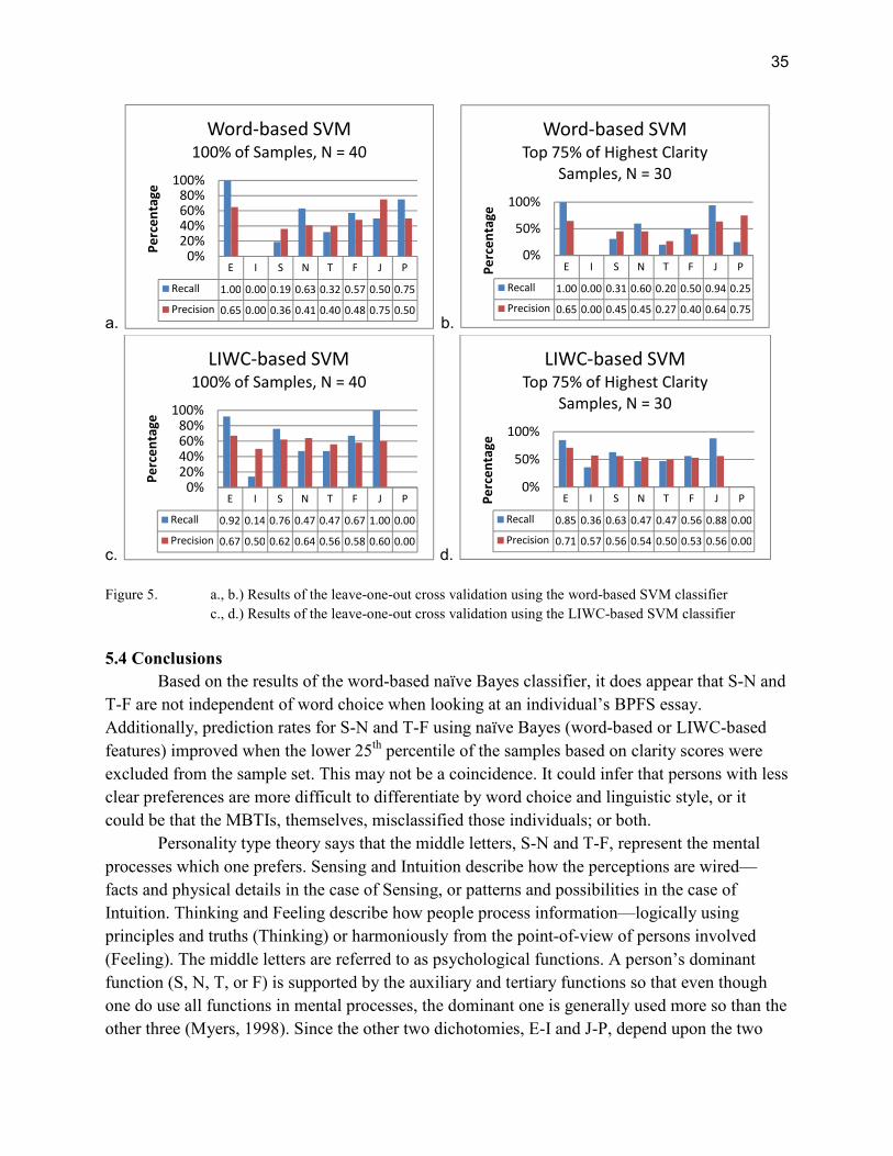
35
a. b.
c. d.
Figure 5. a., b.) Results of the leave-one-out cross validation using the word-based SVM classifier
c., d.) Results of the leave-one-out cross validation using the LIWC-based SVM classifier
5.4 Conclusions
Based on the results of the word-based naïve Bayes classifier, it does appear that S-N and
T-F are not independent of word choice when looking at an individual’s BPFS essay.
Additionally, prediction rates for S-N and T-F using naïve Bayes (word-based or LIWC-based
features) improved when the lower 25th
percentile of the samples based on clarity scores were
excluded from the sample set. This may not be a coincidence. It could infer that persons with less
clear preferences are more difficult to differentiate by word choice and linguistic style, or it
could be that the MBTIs, themselves, misclassified those individuals; or both.
Personality type theory says that the middle letters, S-N and T-F, represent the mental
processes which one prefers. Sensing and Intuition describe how the perceptions are wired—
facts and physical details in the case of Sensing, or patterns and possibilities in the case of
Intuition. Thinking and Feeling describe how people process information—logically using
principles and truths (Thinking) or harmoniously from the point-of-view of persons involved
(Feeling). The middle letters are referred to as psychological functions. A person’s dominant
function (S, N, T, or F) is supported by the auxiliary and tertiary functions so that even though
one do use all functions in mental processes, the dominant one is generally used more so than the
other three (Myers, 1998). Since the other two dichotomies, E-I and J-P, depend upon the two
E I S N T F J P
Recall 1.00 0.00 0.19 0.63 0.32 0.57 0.50 0.75
Precision 0.65 0.00 0.36 0.41 0.40 0.48 0.75 0.50
0%20%40%60%80%
100%
Percentage
Word-based SVM100% of Samples, N = 40
E I S N T F J P
Recall 1.00 0.00 0.31 0.60 0.20 0.50 0.94 0.25
Precision 0.65 0.00 0.45 0.45 0.27 0.40 0.64 0.75
0%
50%
100%
Percentage
Word-based SVMTop 75% of Highest Clarity
Samples, N = 30
E I S N T F J P
Recall 0.92 0.14 0.76 0.47 0.47 0.67 1.00 0.00
Precision 0.67 0.50 0.62 0.64 0.56 0.58 0.60 0.00
0%20%40%60%80%
100%
Percentage
LIWC-based SVM100% of Samples, N = 40
E I S N T F J P
Recall 0.85 0.36 0.63 0.47 0.47 0.56 0.88 0.00
Precision 0.71 0.57 0.56 0.54 0.50 0.53 0.56 0.00
0%
50%
100%
Percentage
LIWC-based SVMTop 75% of Highest Clarity
Samples, N = 30

36
middle letters to a great extent, one entertains the possibility that the dominance of T-F and S-N
is the reason why the middle letters performed better in the classification trials.
LIWC-based features did not result in an accuracy of greater than 70% in any dichotomy.
One explanation for this performance is based on the context of the study. LIWC supporters have
primarily used the Five Factor Model to develop and test LIWC; however, better correlations
between the FFM and the MBTI were achieved through gender-differentiation in a study by
McCrae & Costa (1989). In light of this fact, word-choice alone proved to be the stronger
discriminator, but introducing gender or other data may improve LIWC-based personality type
classification. External factors, such as age, subject reactivity, and first-language may be strong
factors in such assessments, but much more data will need to be collected if such hypotheses are
to be tested. The accuracy in classifying E-I had not improved when using the LIWC-based
feature set with the naïve Bayes classifier. This could be linked to the number of samples relative
to Introversion (only 14).
There is some evidence that naïve Bayes may outperform SVMs when the feature space
is large enough and sample size is small (Ng & Jordan, 2002). The results using naïve Bayes
reflect on its ability to classify text, but its accuracies may also be due to Lidstone smoothing
which helped overcome the unbalanced data using leave-one-out cross-validation on the training
set to select the best values to account for unseen words in the classification task. Thus, data
smoothing played an integral role in stochastically classifying personality types by word-choice.
It is possible that, given a much larger corpus of data, more complex methods of smoothing, such
as Witten-Bell or Good-Turing, will outperform additive smoothing.
In the case of the Support Vector Machines, several kernels and parameters were used in
early experimentation. However, the best configurations resulted in performance no better than
random choice in word-based and LIWC-based SVM classifications. The E-I group consisted of
26 Es and 14 Is which could make E-I very difficult to differentiate by any of the classifiers even
with various methods of weighting. Although weightings may be used in word-based SVM
classification to improve results for unbalanced data, one might conjecture that time would be
better spent in collecting more samples to offset this unbalance and bring the data closer to
population norms. Then, it is likely that the SVM would perform better with a greater number of
samples, given the thousands of features found in these essays.
Poor results for E-I, and to a lesser extent J-P, could be related to smoothing and the
sparseness of the data, or quite possibly, blame might lie with the selection of the essay, itself,
which may not elicit those differences in preference between Extraversion and Introversion.
Thus, essay choice may be a strong factor in classification of some dichotomies more than
others. Diaries, e-mails, and answers to specific questions could be a better discriminator for
some preferences more than others. The decision to use the Best Possible Future Self writing
exercise was based on its richness and ambiguity. However, the selection of the essay may be a
prime factor in the outcome of the experiment. Overall, the results of the naïve Bayes classifier,
in its ability to differentiate documents based on the functional dichotomies, signify its utility in
future studies.

37
5.5 Future Work
Ideally, the number of submissions would number in the thousands for single-label binary
classification of the dichotomies. Gender may be a key factor in differentiating personality type
based on word choice. Education-level, age, ethnicity, first language, region, and even religion
may also have an impact on word-choice that could help improve the performance of any
classifier. Many measures would need to be taken to protect the privacy of such individuals.
It may also be the case that the question (or writing exercise) affects what personality
types one is able to deduce. Further studies should engage the participants in several forms of
writing, personal and non-personal. Context also relates to location, as essays are conducted in a
classroom setting, and participants knew that their essays would be read by someone else.
Linguistic factors might play a part to increase performance, such as parts-of-speech,
tense, quantifiers, and word sense. One may find that an arbitrary personality preference is
disposed to using past tense verbs, or some less tractable feature such as organization may
provide insight. To an extent, LIWC does take into account part-of-speech, tense, and
quantification, but more advanced methods for determining these traits may be employed. Word
sense, though most difficult, would likely offer the most information about an individual’s
thought processes through writing.
In modern exams, such as the G.R.E., natural language processing is a welcome
component. Thus, application of these methods for a variety of means is approaching.
Personality type differences may be quintessential ingredients to an individual’s learning styles
(L.J. Mason, personal communication, July 11, 2011). Brightman (2010) discusses the learning
preferences of students based on personality preferences and addresses some of these concerns,
which all teachers should find interesting and useful. Niesler and Wydmuch (2009) construct a
plausible model for tutoring based on Myers-Briggs personality type, but to identify personality
types, they rely on either deductive logic using user behavior or through the MBTI assessments,
themselves.
Text-based analysis may help to alleviate the problem of identifying personality
preferences for type-based tutoring software in a variety of disciplines since linguistic models
may be more convenient than creating behavior-driven models or implementing the MBTIs,
themselves. Software taking advantage of text-based classification could improve the ability of
modern assessments to recognize these types based on word-choice; the software could also take
advantage of type-based methods for tutoring; lastly, it could take on the form of new human-
computer interaction models.
Future endeavors using the Myers-Briggs typology could have a large impact on how
people interact with machines, appealing to the preferences of an individual to better facilitate
learning and dialogue between humans and computers. Word-based interactions are especially
important in this sense because of the ambiguity of language. Such studies could lead to new
ways of thinking regarding human-computer interaction and possibly improve the user’s
experience with software at work and at home. Such ideas appeal to the very heart of decision-
making and lead to exciting possibilities for anthropomorphic artificial intelligences.

38
References
Allport, G. W. (1937). The Functional autonomy of motives. The American Journal of
Psychology, 50.1/4. EBSCO.
Bird, S., Loper, E., & Klein, E. (2010, November). Natural Language Toolkit. Retrieved from
http://www.nltk.org
Boeree, G. (2004). The evolution of English. Shippensburg University. Retrieved from
http://webspace.ship.edu/cgboer/evolenglish.html
Brightman, H.J. (2010). Master Teaching Program: On learning styles. Master Teaching
Program. Georgia State University. Retrieved from
http://www2.gsu.edu/~dschjb/wwwmbti.html
Call, M. E. & Sotillo, S. (2010). Personality, culture, and field sensitivity. Type and Culture
Intro. Montclair State College. Retrieved from
http://typeandculture.org/Pages/Bibliography.html
Center for Applications of Psychological Type [CAPT]. (2010). Jung's theory of psychological
types and the MBTI® instrument. Retrieved from http://www.capt.org/take-mbti-
assessment/mbti-overview.htm
Chen, S. F. & Goodman, J. (1999). An empirical study of smoothing techniques for language
modeling. Computer Speech & Language, 13.4, 359-93.
Chang, C. C. & Lin, C. J. (2011). LIBSVM : A library for support vector machines. ACM
Transactions on Intelligent Systems and Technology, 2.27, 1-27. Retrieved from
http://www.csie.ntu.edu.tw/~cjlin/libsvm
Chung, C.K. & Pennebaker, J.W. (2007). The psychological function of function words. Social
communication: Frontiers of Social Psychology, 343-359. New York, NY: Psychology
Press.
Chung, C.K. & Pennebaker, J.W. (2008). Revealing dimensions of thinking in open-ended self-
descriptions: An automated meaning extraction method for natural language. Journal of
Research in Personality, 42.1, 96-132.
Cortes, C. & Vapnik, V. (1995). Support-vector networks. Machine Learning, 20.3, 273-97.
Elisseeff, A. & Pontil, M. (2003). Leave-one-out error and stability of learning algorithms with
applications. Learning Theory and Practice. IOS Press.
Fletcher, T. (2009, March 1). Support vector machines explained. University College London.
Retrieved from http://www.tristanfletcher.co.uk/SVM%20Explained.pdf
Furnham, A. (1996). The big five versus the big four: The relationship between the Myers-
Briggs Type Indicator (MBTI) and NEO-PI Five Factor Model of personality.
Personality and Individual Differences 21.2, 303-307.
39
Heckerman, D. (1995, March). A tutorial on learning with Bayesian networks. Microsoft
Research Technical Report, MSR-TR-95-06. Retrieved from
http://research.microsoft.com/apps/pubs/default.aspx?id=69588
Jiang, L., Zhang, H., & Cai, Z. (2009). A novel Bayes model: Hidden naïve Bayes. IEEE
Transactions on Knowledge and Data Engineering 21.10, 1361-371.
Jurafsky, D. & Martin, J.H. (2009). Speech and Language Processing: An Introduction to Natural
Language Processing, Speech Recognition, and Computational Linguistics. 2nd edition.
Prentice-Hall.
Kalu, E., Kaw, A., & Nguyen, C. (2010, April). Linear regression. University of South Flordia.
Retrieved from http://numericalmethods.eng.usf.edu
Kim, S.B., Han, K.S., Rim, H.C., & Myaeng, S.H. (2006). Some effective techniques for naïve
Bayes text classification. IEEE Transactions on Knowledge and Data Engineering 18.11,
1457-466.
King, L. A. (2001). The health benefits of writing about life goals. Personality and Social
Psychology Bulletin, 27.7, 798-807.
Lee, A., Caron, F., Docet, A., & Holmes, C. (2010, September 16). A hierarchical Bayesian
framework for constructing sparsity-inducing priors. Cornell University Library.
Retrieved from http://arxiv.org/abs/1009
Lee, C., Kim, K., Seo, Y., & Chung, C. (2007). The relations between personality and language
use. The Journal of General Psychology, 134.4, 405-13
Li, L. (2007, September 18). Bayesian classification and regression with high dimensional
features. Department of Statistics, University of Toronto. Retrieved from
http://www.db.toronto.edu/~radford/ftp/longhai-thesis1.pdf
McCallum, A. & Nigam, K. (1998). A comparison of event models for naïve Bayes text
classification. AAAI/ICML ‘98 Workshop of Learning for Text Categorization. Retrieved
from http://www.cs.cmu.edu/~knigam/papers/multinomial-aaaiws98.pdf
McRae, R. & Costa, P. (1989). Reinterpreting the Myers-Briggs Type Indicator from the
perspective of the Five-Factor Model of personality. Journal of Personality, 57.1, 17-40.
Mehl, M.R. & Pennebaker, J.W. (2003). The sounds of social life: A psychometric analysis of
students' daily social environments and natural conversations. Journal of Personality and
Social Psychology, 84, 857-870.
Mierswa, I., Wurst, M., Klinkenberg, R., Scholz, M., & Euler, T. (2010). RapidMiner
Community Edition. Rapid-i. Retrieved from http://rapid-i.com/
Miller, G.A., Fellbaum, C., & Tengi, R. (2010). WordNet Lexical Database. Princeton
Univerisity. Retrieved from http://wordnet.princeton.edu

40
Miller, W. G. (2010, November 22). OpenStat Advanced Statistical Package. Retrieved from
http://statpages.org/miller/openstat/
Myers, I. (1998). MBTI Manual: A guide to the development and use of the Myers-Briggs Type
Indicator. Palo Alto, CA: Consulting Psychologists.
Niesler, A. & Wydmuch, G. (2009). User profiling in intelligent tutoring systems based on
Myers-Briggs personality types. Proceedings of the International MultiConference of
Engineers and Computer Scientists. Hong Kong: 1, Table 1. Retrieved from
Newton, A. T., Kramer, A. D., & McIntosh, D. N. (2009). Autism online: A comparison of word
usage in bloggers with and without autism spectrum disorders. In Proceedings of the 27th
International Conference on Human Factors in Computing Systems (Boston, MA, USA,
April 04 - 09, 2009). CHI '09, 463-466.
Ng, A. Y. & Jordan, M. (2002). On discriminative vs. generative classifers: A comparison of
logistic regression and naïve Bayes. Neural Information Processing Systems, 14.
Pearl, J. (1986). Fusion, propagation, and structuring in belief networks. Artificial Intelligence,
29.3, 241-88.
Pennebaker, J. W. (2002, January). What our words can say about us: Toward a broader
language psychology. Psychological Science Agenda, 8-9.
Pennebaker, J.W., Francis, M.E., & Booth, R.J. (2007). LIWC 2007 Windows Application,
v.1.08. Mahwah, N.J.: LEA Software and Alternative Media, Inc.
Pennebaker, J. W. & King, L. A. (1999). Linguistic styles: Language use as an individual
difference. Journal of Personality and Social Psychology, 77.6, 1296-312.
Pennebaker, J.W., Mehl, M.R., & Niederhoffer, K.G. (2003). Psychological aspects of natural
language use: Our words, our selves. Annual Review of Psychology, 54.1, 547-77.
Pennebaker, J. W. (2001). Patterns of natural language use: Disclosure, personality, and social
integration. Current Directions in Psychological Science, 10.3. American Psychological
Society.
Porter, M.F. (1980, July). An algorithm for suffix stripping, Program, 14.3, 130–137. Retrieved
from http://tartarus.org/~martin/PorterStemmer/def.txt
Rennie, J., Shih, L., Teevan, J., & Karger, D. (2003). Tackling the poor assumptions of naïve
Bayes text classifiers. Proceedings of the Twentieth International Conference on
Machine Learning. Retrieved from http://lingpipe-blog.com/2009/02/16/rennie-shih-
teevan-and-karger-2003-tackling-poor-assumptions-naive-bayes-text-classifiers/
Rish, I. (2001). An empirical study of the naive Bayes classifier. International Joint Conference
on Artificial Intelligence: Workshop on empirical methods in artificial intelligence.
Yorktown Heights, NY: Thomas J. Watson Research Center.

41
Rude, S.S., Gortner, E.M., & Pennebaker, J.W. (2004). Language use of depressed and
depression-vulnerable college students. Cognition and Emotion, 18, 1121-1133.
Schaubhut, N.A., Herk, N.A., & Thompson, R.C. (2009). MBTI form M manual supplement.
Mountain View, CA: CPP, Inc. Retrieved from
https://www.cpp.com/pdfs/MBTI_FormM_Supp.pdf 10 Nov. 2010
Sebastiani, F. (2001). Machine learning in automated text categorization. Rome, Italy: Consiglio
Nazionale delle Ricerche. Retrieved from
http://nmis.isti.cnr.it/sebastiani/Publications/ACMCS02.pdf
Smyth, J. M. (1998). Written emotional expression: Effect sizes, outcome types, and moderating
variables. Journal of Consulting and Clinical Psychology, 66.1, 174-184
Soboroff, I., Nicholas, C., Kukla, J., & Ebert, D (1997). Visualizing document authorship using
n-grams and latent semantic indexing. University of Maryland. Retrieved from
http://www.cs.umbc.edu/~ian/pubs/hlsi.ps.gz
Spera, S.P., Buhrfiend, E.D., & Pennebaker, J.W. (1994). Expressive writing and coping with
job loss. Academy of Management Journal, 37.3, 722-33.
Quenk, N.L., Hammer, A.L., & Majors, M.S. (2001). MBTI Step II manual: Exploring the next
level of type with the Myers-Briggs Type Indicator form Q. Mountain View, CA: CPP,
Inc.
Tausczik, Yla R. & J. W. Pennebaker (2010). The psychological meaning of words: LIWC and
computerized text analysis methods. University of Texas, Austin. Retrieved from
http://homepage.psy.utexas.edu/HomePage/Faculty/Pennebaker/Reprints/Tausczik&Penn
ebaker2010.pdf
Tupes, E.C. & Cristal, R.E. (1961). Recurrent personality factors based on trait ratings.
Armstrong Laboratory, Aeronautical Systems Division. ASD-TR-61-97. EBSCO.
Tzeng, O., Ware, R., & Chen, J.M. (1989). Measurement and utility of continuous unipolar
ratings for the Myers-Briggs Type Indicator. Journal of Personality Assessment, 53.4,
727-38.
Walsh, C. B. (2004, April). Markov Chain Monte Carlo and Gibbs sampling. Lecture Notes for
EEB 581. Massachusetts Institute of Technology. Retrieved from
http://web.mit.edu/~wingated/www/introductions/mcmc-gibbs-intro.pdf
Williams, T. & Kelley, C. (2004). Gnuplot, v.4.2.6. Retrieved from http://gnuplot.info
Witten, I.H. & Bell, T.C. (1991). The Zero Frequency Problem: Estimating the probabilities of
novel events in adaptive text compression. IEEE Transactions on
Information Theory, 37.4, 1085–1094.
Weisstein, E. W. (2010). Poisson distribution. Wolfram MathWorld. Retrieved from
http://mathworld.wolfram.com/PoissonDistribution.html

Appendix A: Descriptions of the Personality Type Dichotomies
Note. From the MBTI Manual: A guide to the development and use of the Myers-Briggs Type Indicator (Myers,
1998).

43
Appendix B: Descriptions of the 16 Psychological Types
Note. From the MBTI Manual: A guide to the development and use of the Myers-Briggs Type Indicator (Myers,
1998).

44
Appendix C. Sample Myers-Briggs Type Indicator Step II Report (MBTI)
Note. From the MBTI form M manual supplement (Schaubhut et al, 2009).

45
Appendix D. Scores of Participants Using the MBTI Step II
Table 9
Scores of participants using the MBTI Step II
File Type E I S N T F J P
101 ESFJ 24 9 17 28 102 ISTJ 5 2 5 14 103 ISTJ 14 24 1 22 104 ENFP 24 21 24 18 105 ISFJ 26 4 8 1 106 ENFJ 19 23 4 17 108 ESFJ 12 8 4 21 109 ENFP 25 10 10 18 110 ESTP 26 5 11 30 111 ISTP 1 13 18 6 112 ENTJ 19 8 23 2 113 ESTP 9 2 7 5 201 ISTP 2 16 3 18 202 ENFJ 15 16 6 1 203 ENTJ 5 1 11 2 204 INTP 1 14 20 9 205 INFJ 10 8 8 23 206 ENTP 20 16 6 1 207 ENFP 13 30 17 4 208 INFP 9 13 1 10 209 ENFP 10 18 13 17 210 ESFJ 11 4 2 16 301 ENFP 9 30 19 26 302 ISTJ 6 7 16 18 303 ISFJ 25 11 6 24 304 ESFP 30 17 26 6 305 ESTJ 3 19 5 30 306 ESTJ 23 7 8 13 307 ENFP 28 9 3 22 308 ENTJ 12 11 9 18 309 ESFJ 21 3 12 20 310 ISTJ 6 5 6 8 311 ESFP 30 3 15 15 312 ENTJ 30 7 22 15 313 INTJ 5 15 1 7 314 ESTJ 30 20 11 17 315 ISTJ 16 6 8 4 316 ENFP 9 14 1 13 317 ENFJ 6 1 1 5 318 ISFJ 3 24 8 22
Note. Clarity scores may fall within the range of 0 to 30 for each preference.

46
Appendix E. Search for Optimal Values of C and Gamma Using LibSVM
Note. Optimization visualized in Gnuplot (Williams & Kelly, 2004) using libSVM’s grid.py (Chang & Lin 2011).
Accuracy depicts the results of k-fold cross-validation on the training set to optimize c and gamma, i.e. the
parameters to C-SVC.

47
Appendix F. Stop-word Corpus Used in Word-based Classification Trials
Table 10
NLTK English stop-word corpus
Stop-words
i which because further t
me who as then can
my whom until once will
myself this while here just
we that of there don
our these at when should
ours those by where now
ourselves am for why
you is with how
your are about all
yours was against any
yourself were between both
yourselves be into each
he been through few
him being during more
his have before most
himself has after other
she had above some
her having below such
hers do to no
herself does from nor
it did up not
its doing down only
itself a in own
they an out same
them the on so
their and off than
theirs but over too
themselves if under very
what or again s Note. In practice, words are converted to lower case before stop-
word filtering. The corpus included with the Natural Language
Toolkit consists of 127 stop-words. (Bird et al., 2010)

48
Appendix G. Proposed Fix for a Logic Error in the NLTK Python Module
File: ..\Python26\Lib\site-packages\nltk\probability.py
Method: WittenBellProbDist.
Logic Error (self._Z will always be zero) BEGIN PYTHON CODE
assert bins == None or bins >= freqdist.B(),\
'Bins parameter must not be less than freqdist.B()'
if bins == None:
bins = freqdist.B()
self._freqdist = freqdist
self._T = self._freqdist.B()
self._Z = bins - self._freqdist.B()
self._N = self._freqdist.N()
# self._P0 is P(0), precalculated for efficiency:
if self._N==0:
# if freqdist is empty, we approximate P(0) by a UniformProbDist:
self._P0 = 1.0 / self._Z
else:
self._P0 = self._T / float(self._Z * (self._N + self._T))
END CODE
Proposed Changes BEGIN PYTHON CODE
assert bins == None or bins >= freqdist.B(),\ 'Bins parameter must not be less than freqdist.B()'
if bins == None:
self._Z = freqdist.B()
else:
self._Z = bins - self._freqdist.B()
END CODE
Note. Code from probability.py in the Natural Language Toolkit (Bird et al., 2010).

49
Appendix H. Results of the Classification Decisions by Document
Table 11
Results of Classification by Document for E-I
SVM Naïve Bayes
File Type LIWC-based Word-based Word-based LIWC-based
101 E 1 1 1 1
104 E 1 1 0 1
106 E 1 1 1 1
108 E 0 1 1 1
109 E 1 1 0 1
110 E 1 1 0 1
112 E 1 1 1 1
113* E 1 1 0 1
202 E 1 1 1 1
203* E 1 1 0 1
206 E 1 1 0 1
207 E 1 1 1 1
209 E 1 1 1 1
210 E 1 1 1 1
301* E 1 1 1 1
304 E 1 1 1 0
305 E 1 1 0 1
306 E 1 1 1 1
307 E 1 1 1 0
308 E 1 1 0 1
309 E 1 1 1 1
311 E 1 1 1 1
312 E 0 1 0 1
314 E 1 1 0 1
316* E 1 1 1 1
317* E 1 1 0 1
102 I 0 0 0 0
103 I 0 0 1 0
105 I 0 0 0 0
111* I 0 0 0 0
201* I 0 0 0 0

50
Table 11 cont.
204* I 0 0 0 0
205 I 1 0 0 0
208 I 1 0 0 0
302 I 0 0 0 1
303 I 0 0 0 0
310 I 0 0 0 0
313 I 0 0 0 0
315 I 0 0 0 0
318 I 0 0 0 0
*Essay by an author whose clarity score falls within the lower 25th
percentile in group
Note. A correct prediction is labeled 1 and mispredictions are labeled 0.
Table 12
Results of Classification by Document for S-N
SVM Naïve Bayes
File Type LIWC-based Word-based Word-based LIWC-based
104 N 1 0 1 1
106 N 1 1 1 1
109 N 1 1 1 1
112* N 0 0 0 0
202 N 1 1 1 1
203* N 1 0 0 1
204 N 0 1 1 1
205 N 0 1 0 1
206 N 0 1 1 0
207 N 1 1 1 0
208 N 1 1 1 1
209 N 0 1 1 1
301 N 1 1 1 1
307 N 0 0 1 0
308 N 0 0 0 1
312* N 0 0 1 0
313 N 0 1 0 0
316 N 0 0 0 0
317* N 1 1 1 1
101 S 1 1 0 1
102* S 0 0 0 0

51
Table 12 cont.
103 S 1 0 1 0
105* S 1 0 0 0
108 S 1 0 1 1
110 S 1 0 1 1
111 S 0 0 1 0
113* S 1 0 1 1
201 S 1 0 1 1
210 S 1 1 1 1
302 S 1 0 1 1
303 S 0 0 1 0
304 S 1 1 1 1
305 S 0 0 1 0
306 S 1 0 0 0
309* S 1 0 0 0
310 S 0 1 1 1
311* S 1 0 0 0
314 S 1 0 1 1
315 S 1 0 1 1
318 S 1 0 1 0
*Essay by an author whose clarity score falls within the lower 25th
percentile in group
Note. A correct prediction is labeled 1 and mispredictions are labeled 0.
Table 13
Results of Classification by Document for T-F
SVM Naïve Bayes
File Type LIWC-based Word-based Word-based LIWC-based
101 F 1 0 0 0
104 F 0 1 0 0
105 F 1 1 0 1
106 F 1 0 0 1
108 F 1 1 0 0
109 F 0 0 1 1
202 F 1 1 1 1
205 F 0 0 1 1
207 F 1 1 1 1
208* F 1 1 1 1
209 F 1 0 1 1
210* F 1 1 0 1

52
Table 13 cont.
301 F 1 1 1 1
303 F 1 0 1 1
304 F 0 0 1 0
307* F 0 0 1 0
309 F 1 0 0 0
311 F 0 1 0 0
316* F 1 1 0 0
317* F 1 1 0 0
318 F 0 1 1 0
102* T 1 0 0 0
103* T 0 0 0 0
110 T 0 1 0 1
111 T 0 0 0 0
112 T 0 0 0 0
113 T 0 0 1 1
201* T 1 1 1 1
203 T 1 0 0 1
204 T 1 1 0 0
206 T 1 0 1 1
302 T 0 1 1 1
305 T 0 0 0 1
306 T 1 1 1 0
308 T 0 0 0 0
310 T 1 0 1 1
312 T 0 0 1 0
313* T 0 0 1 1
314 T 1 0 1 1
315 T 1 1 1 1
*Essay by an author whose clarity score falls within the lower 25th
percentile in group
Note. A correct prediction is labeled 1 and mispredictions are labeled 0.

53
Table 14
Results of Classification by Document for J-P
SVM Naïve Bayes
File Type LIWC-based Word-based Word-based LIWC-based
101 J 1 1 1 1
102 J 1 1 1 1
103 J 1 1 1 1
105* J 1 0 0 1
106 J 1 1 0 1
108 J 1 1 1 1
112* J 1 0 1 1
202* J 1 1 0 1
203* J 1 0 1 1
205 J 1 0 1 1
210 J 1 0 1 0
302 J 1 0 0 1
303 J 1 1 1 1
305 J 1 1 0 1
306 J 1 1 1 1
308 J 1 1 0 1
309 J 1 0 1 1
310 J 1 0 1 1
312 J 1 0 0 1
313 J 1 0 1 1
314 J 1 1 0 1
315* J 1 0 0 1
317* J 1 0 1 1
318 J 1 1 1 1
104 P 0 1 0 0
109 P 0 0 1 0
110 P 0 0 1 0
111 P 0 0 0 0
113* P 0 1 0 0
201 P 0 1 0 0
204 P 0 1 1 0
206* P 0 1 0 0
207* P 0 1 1 0

54
Table 14 cont.
208 P 0 1 1 0
209 P 0 1 0 0
301 P 0 1 1 0
304* P 0 1 0 0
307 P 0 1 1 1
311 P 0 1 1 0
316 P 0 0 0 0
*Essay by an author whose clarity score falls within the lower 25th
percentile in group
Note. A correct prediction is labeled 1 and mispredictions are labeled 0.
Table 15
Results of Subgroup Classification by Document for E-I
SVM Naïve Bayes
File Type LIWC-based Word-based Word-based LIWC-based
101 E 0 1 1 1
104 E 1 1 0 1
106 E 1 1 1 1
108 E 1 1 0 1
109 E 1 1 1 1
110 E 1 1 0 1
112 E 1 1 0 1
202 E 1 1 1 1
206 E 0 1 0 1
207 E 1 1 1 1
209 E 1 1 0 1
210 E 1 1 0 1
304 E 1 1 1 1
306 E 1 1 1 1
307 E 1 1 0 0
308 E 1 1 1 1
309 E 1 1 0 1
311 E 1 1 0 1
312 E 1 1 1 1
314 E 0 1 1 1
102 I 0 0 0 0
103 I 1 0 1 0
105 I 0 0 0 0

55
Table 15 cont.
205 I 0 0 0 0
208 I 1 0 0 0
302 I 0 0 0 0
303 I 1 0 0 0
310 I 0 0 0 0
313 I 1 0 0 0
315 I 0 0 0 0
318 I 0 0 0 0
Note. A correct prediction is labeled 1 and mispredictions are labeled 0.
Table 16
Results of Subgroup Classification by Document for S-N
SVM Naïve Bayes
File Type LIWC-based Word-based Word-based LIWC-based
104 N 0 1 1 1
106 N 0 1 1 1
109 N 1 1 1 1
202 N 1 1 1 1
204 N 0 1 1 1
205 N 0 0 0 1
206 N 0 1 1 0
207 N 1 1 1 0
208 N 1 1 1 1
209 N 1 1 1 1
301 N 1 0 1 1
307 N 0 0 1 1
308 N 1 0 0 1
313 N 0 0 0 0
316 N 0 0 0 0
101 S 1 1 1 0
103 S 1 0 1 0
108 S 1 0 1 1
110 S 1 0 0 1
111 S 0 0 1 0
201 S 0 0 1 1
210 S 1 1 1 1
302 S 1 0 1 1

56
Table 16 cont.
303 S 0 0 1 0
304 S 1 1 1 1
305 S 0 0 0 0
306 S 1 1 0 0
310 S 1 1 1 1
314 S 0 0 1 1
315 S 1 0 1 1
318 S 0 0 1 0
Note. A correct prediction is labeled 1 and mispredictions are labeled 0.
Table 17
Results of Subgroup Classification by Document for T-F
SVM Naïve Bayes
File Type LIWC-based Word-based Word-based LIWC-based
101 F 0 0 0 0
104 F 0 0 0 0
105 F 1 0 1 1
106 F 1 1 1 1
108 F 1 1 1 0
109 F 0 0 1 0
202 F 1 1 1 1
205 F 1 1 1 1
207 F 0 1 1 0
209 F 1 1 1 1
301 F 1 0 1 1
303 F 1 1 1 1
304 F 0 0 1 0
309 F 1 0 0 1
311 F 0 0 0 0
318 F 0 1 1 0
110 T 0 0 1 1
111 T 0 0 1 0

57
Table 17 cont.
112 T 0 0 0 0
113 T 0 0 1 1
203 T 1 0 0 1
204 T 0 0 0 0
206 T 1 0 1 1
302 T 0 1 1 1
305 T 1 0 1 1
306 T 1 0 1 0
308 T 0 0 1 0
310 T 1 1 0 1
312 T 1 0 1 0
314 T 0 0 1 1
315 T 1 1 1 1
Note. A correct prediction is labeled 1 and mispredictions are labeled 0.
Table 18
Results of Subgroup Classification by Document for J-P
SVM Naïve Bayes
File Type LIWC-based Word-based Word-based LIWC-based
101 J 1 1 1 1
102 J 1 1 1 1
103 J 1 1 1 1
106 J 1 1 0 1
108 J 1 1 1 1
205 J 1 1 1 1
210 J 1 1 1 0
302 J 1 1 1 1
303 J 1 1 1 1
305 J 0 0 0 0
306 J 1 1 1 1
308 J 1 1 1 1
309 J 1 1 1 1
310 J 1 1 1 1
312 J 0 1 1 0
313 J 1 1 1 1
314 J 1 1 1 1
318 J 1 1 1 1

58
Table 18 cont.
104 P 0 1 0 0
109 P 0 0 1 0
110 P 0 0 1 0
111 P 0 0 0 0
201 P 0 1 0 0
204 P 0 0 1 0
208 P 0 0 1 0
209 P 0 0 1 0
301 P 0 1 1 0
307 P 0 0 1 1
311 P 0 0 1 0
316 P 0 0 0 0
Note. A correct prediction is labeled 1 and mispredictions are labeled 0.