arX
iv:q
uant
-ph/
9812
048v
1 1
7 D
ec 1
998
Matrix Elements for a Generalized
Spiked Harmonic Oscillator
Richard L. Hall, Nasser Saad †
and
Attila B. von Keviczky
Department of Mathematics and Statistics,
Concordia University,
1455 de Maisonneuve Boulevard West,
Montreal, Quebec,
Canada H3G 1M8.
Abstract
Closed form expressions for the singular-potential integrals <m|x−α|n> are obtained
with respect to the Gol’dman and Krivchenkov eigenfunctions for the singular potential
Bx2 + Ax2 , B > 0, A ≥ 0. The formulas obtained are generalizations of those found
earlier by use of the odd solutions of the Schrodinger equation with the harmonic
oscillator potential [Aguilera-Navarro et al, J. Math. Phys. 31, 99 (1990)].
PACS 03.65.Ge
† Present address: Department of mathematics, faculty of science, Notre Dame Uni-
versity, Beirut, Lebanon

Matrix Elements for . . . Page 2
I. Introduction
In 1990 Aguilera-Navarro et al1 employed a perturbative scheme to provide a vari-
ational analysis for the lowest eigenvalue of the Schrodinger operator
H = − d2
dx2+ x2 +
λ
xα, 0 ≤ x <∞,
where α is a positive constant. WritingH ≡ H0+λV withH0 standing for the harmonic
oscillator Hamiltonian and V = x−α, Aguilera-Navarro et al1 used the basis set
ψn(x) = Ane−x2/2H2n+1(x), A−2
n = 22n+1(2n+ 1)!, n = 0, 1, 2, . . . (1)
constructed from the normalized solutions of H0ψ = Eψ to evaluate the matrix ele-
ments of H. They found that
Hm+1,n+1 ≡ (3 + 4n)δm,n + λ<m|x−α|n> m, n = 0, 1, 2, . . . , N − 1, (2)
where
<m|x−α|n> = (−1)n+m
√
(2n+ 1)!(2m+ 1)!
2n+mn!m!
×m
∑
k=0
(−1)k
(
m
k
)
Γ(k + 3−α2
)Γ(n− k + α2)
Γ(k + 32 )Γ(−k + α
2 ).
(3)
The aim of this article is to extend these results to treat the more general spiked
harmonic oscillator Hamiltonian
H = − d2
dx2+Bx2 +
A
x2+
λ
xαB > 0, A ≥ 0. (4)
The particular case of A = 0 and B = 1 allows us, of course, to recover the results of
Aguilera-Navarro et al1 as a special case. The existence of all the exact eigenfunctions
for a problem with a singular potential is the principal motivation for the present
work: we expect that such a set of functions will be more effective for the analysis of
other singular problems than are the Hermite functions generated, as they are, by the
non-singular harmonic-oscillator potential x2.
The article is organized as follows. In Sec. II we provide an orthonormal set of
functions that we use to compute the matrix elements of the Hamiltonian (4). In Sec.
III we prove that this set of functions is complete in the sense that it is a basis for
L2(0,∞). We then compute the matrix elements using this basis in Sec. IV. In Sec. V

Matrix Elements for . . . Page 3
the comparison with the result of Aguilera-Navarro et al1 are presented for the special
case B = 1 and A = 0: where we shall point out some errors in their value for the
matrix element <ψ3|x−α|ψ3> as quoted in the appendix of Ref. [1].
II. An orthonormal basis
Gol’dman and Krivchenkov2 have provided a clear description of the exact solutions of
the following one dimensional Schrodinger equation (in units h = 2m = 1)
−ψ′′ + V0
(
a
x− x
a
)2
ψ = Enψ, x ∈ [0,∞) (5)
with ψ satisfying the Dirichlet boundary condition ψ(0) = 0. They showed that the
energy spectrum in terms of the parameters V0 and a is given by
En =4
a
√
V0
{
n+1
2+
1
4
(
√
1 + 4V0a2 − 2a√
V0
)}
. (6)
To simplify notation we introduce the parameters B = V0a−2 and A = V0a
2, and obtain
thereby an exact solution to the Schrodinger equation with the singular potential
V (x) = Bx2 +A
x2, B > 0, A ≥ 0, (7)
where the energy spectrum is now given in terms of the parameters A and B by
En =√B(4n+ 2 +
√1 + 4A), n = 0, 1, 2, . . . . (8)
The wave functions have the form
<x|n> ≡ ψn(x) = Cnx1
2(1+
√1+4A)e−
1
2
√Bx2
1F1(−n, 1 +1
2
√1 + 4A;
√Bx2), (9)
where n = 0, 1, 2, . . . and 1F1 is the confluent hypergeometric function3
1F1(a, b; z) =∑
k
(a)kzk
(b)kk!.
The Pochhammer symbols (a)k are defined as
(a)k = a(a+ 1)(a+ 2) . . . (a+ k − 1) =Γ(a+ k)
Γ(a), k = 1, 2, . . . (10)

Matrix Elements for . . . Page 4
where Γ(a) is the gamma function. Note that we have corrected the misprint of Ref.
[4] for the power of x in the wavefunctions (9). The constant Cn is determined from
the normalization condition∫ ∞
0
ψ2n(x)dx = 1,
which requires use of the identity4
∞∫
0
e−λxxν−1[1F1(−n, γ; kx)]2dx =n!Γ(ν)
kνγ(γ + 1) . . . (γ + n− 1)
×{
1 +n−1∑
s=0
n(n− 1) . . . (n− s)(γ − ν − s− 1)(γ − ν − s) . . . (γ − ν + s)
[(s+ 1)!]2γ(γ + 1) . . . (γ + s)
}
,
(11)
thereby yielding
C2n =
2B1
2+ 1
4
√1+4AΓ(n+ 1 + 1
2
√1 + 4A)
n![Γ(1 + 12
√1 + 4A)]2
. (12)
In order to prove that the ψn(x), n = 0, 1, 2, . . . , defined by (9) are orthonormal, we
have to demonstrate∞∫
0
ψn(x)ψm(x)dx = 0 (n 6= m). (13)
We know however, that ψn(x) and ψm(x) satisfy the Schrodinger equations
ψ′′n + (En −Bx2 − A
x2)ψn = 0, En =
√B(4n+ 2 +
√1 + 4A), (14)
ψ′′m + (Em −Bx2 − A
x2)ψm = 0, Em =
√B(4m+ 2 +
√1 + 4A). (15)
Multiplying (14) by ψm and (15) by ψn and then subtracting the resulting equations,
we obtaind
dx(ψmψ
′n − ψnψ
′m) +
√B(n−m)ψnψm = 0.
After integrating this equation over [0,∞) and using ψn(0) = ψm(0) = 0 and ψn(∞) =
ψm(∞) = 0, we get
(n−m)
∞∫
0
ψn(x)ψm(x)dx = 0,
which proves (13). Thus we obtain the following identity

Matrix Elements for . . . Page 5
∞∫
0
e−λx2
x2γ−11F1(−n, γ;λx2)1F1(−m, γ;λx2)dx =
0 if n 6= m,
1
2
n!Γ(γ)
λγ(γ)nif n = m,
wherein the confluent hypergeometric functions 1F1 are defined as follows3:
1F1(−n, γ; r) ≡ − 1
2πi
Γ(n+ 1)Γ(γ)
Γ(n+ γ)
∮
C′
ˆ etr(−t)−n−1(1 − t)γ−n−1dt =
Γ(γ)
Γ(γ + n)r1−γerDn(rγ+n−1e−r) =
Γ(γ)
Γ(γ + n)r1−γ(D − 1)n(rγ+n−1) (16)
for any simply closed rectifiable contour C′ starting at 1 and enclosing the straight
line segment from 0 to 1 in the complex plane, as illustrated in Fig. 1. With γ =
1 + 12
√1 + 4A and λ =
√B, the set of L2(0,∞)-functions
ψn(x) = Cnxγ− 1
2 e−1
2λx2
1F1(−n, γ;λx2), n = 0, 1, 2, . . . (17)
constitutes a orthonormal system of the Hilbert space L2(0,∞).
III. Proof of Completeness
For the orthonormal functions {ψn} to qualify as a basis for L2(0,∞), we must
demonstrate the density of the linear manifold generated by these functions in the
topology induced by the norm determined by the inner product < · | · >. This is
equivalent to showing that if < ψn|f >= 0 for all n = 0, 1, 2, . . ., then f = 0 a.e. on
(0,∞). To this end we note that out of the fourth expression of (16) follows
1F1(−n, γ;λx2) =
n∑
k=0
(
n
k
)
(−λ)n−kΓ(γ)
Γ(γ + n− k)x2(n−k). (18)
Hence the basis representation of the functions (vectors)
{1F1(−n, γ;λx2), 1F1(−(n− 1), γ;λx2), . . . , 1F1(−1, γ;λx2), 1F1(−0, γ;λx2)}
in terms of the basis
{x2n, x2(n−1), . . . , x2, 1}
Matrix Elements for . . . Page 6
is achieved by a lower triangular (n+ 1) × (n+ 1) matrix, whose diagonal entries are(−λ)n−kΓ(γ)Γ(γ+n−k) for k = 0, 1, 2, . . . , n - i.e. this matrix is invertible provided λ 6= 0. Thus
each x2n is a unique linear combination of the n+1 functions 1F1(−(n−k), γ;λx2) for
k = 0, 1, 2, . . . , n, which conclusion carries over to the 2n-th degree Taylor polynomial
en(−µx2
2) =
n∑
k=0
1
k!
(
− µx2
2
)k
of e−µx2
2 about the point 0, where µ is an arbitrary parameter.
Let f be an L2(0,∞)-function orthogonal to each of the ψn, which is equivalent to
saying
< en(−µ · 2
2)|f >=
∞∫
0
xγ− 1
2 en(−µx2
2)f(x)dx = 0 (19)
for all n = 0, 1, 2, . . .. Here we note that
xγ− 1
2 e−λx2
4 f(x)
in an L1(0,∞)-function whose absolute value majorizes xγ− 1
2 e−λx2
4 e|µ|x2
4 f(x) for |µ| ≤λ4 and consequently also xγ− 1
2 e−λx2
4 en(−µx2/4)f(x).
Because xγ− 1
2 e−λx2
4 en(−µx2/4)f(x) converges to xγ− 1
2 e−λx2
2 f(x) a.e. on (0,∞) as
n→ ∞, we conclude by means of the Lebesgue dominated convergence theorem5 that
we may replace en(−µx2/2) by e−µx2
2 in Eq.(19) for all complex numbers µ such that
|µ| ≤ λ4 , which, after setting x =
√2t, yields the Laplace-Transform expression
L{F}(z) =
∞∫
0
e−zt(√
2t)γ− 3
2 f(√
2t)dt = 0, |z − λ| ≤ λ
4. (20)
However, the Laplace transform of the measurable Laplace-transformable function
F (t) = e−zt(√
2t)γ− 3
2 f(√
2t) defines a holomorphic function of variable z in the right
half plane ℜ(z) > 0 vanishing in the disc |z − λ| ≤ λ4 . By uniqueness of the analytic
function6 the Laplace transform of the function must vanish in the right half plane,
specifically L{F}(s) = 0 for all s on the interval (0,∞). Further, the Laplace trans-
form determines F (t) uniquely7 a.e. in t on (0,∞), hence F (t) = 0 a.e. in t or f is the
zero L2(0,∞)-function. Consequently, {ψn : n = 0, 1, 2, . . .} is an orthonormal basis of
L2(0,∞).
Matrix Elements for . . . Page 7
IV. The matrix elements <m|x−α|n>Let us now split the Hamiltonian (5) into an H0 part
H0 = − d2
dx2+Bx2 +
A
x2, x ≥ 0 (21)
and a perturbation
HI = λ/xα.
The eigenstates of H0 are now given by (9) and their unperturbed energy is given by
(8). All we need to do is to evaluate the matrix elements < m|x−α|n > using the basis
(9), namely
< m|x−α|n >=CnCm
∞∫
0
e−√
Bx2
x−α+1+√
1+4A1F1(−n, 1 +
1
2
√1 + 4A;
√Bx2)
× 1F1(−m, 1 +1
2
√1 + 4A;
√Bx2)dx,
α < 2 +√
1 + 4A
(22)
This is equivalent to
< m|x−α|n >=CnCm
2B− 1
2(−α+2+
√1+4A) × I, (23)
where
I =
∞∫
0
e−rrγ−s1F1(−n, γ; r)1F1(−m, γ; r)dr (24)
with r =√Bx2, γ = 1 + 1
2
√1 + 4A, and s = 1 + α
2 .
¿From the Fubini-Tonneli theorem5 combined with the Leibniz formula for dif-
ferentiating the product of two functions, as well as exponential shift from the third
expression to the fourth in Eq.(16), with n replaced by m, we find that I is given by
the expression
I = (−1)n n![Γ(γ)]2
Γ(n+ γ)Γ(m+ γ)(2πi)−1
∮
C′
ˆ t−n−1(1 − t)γ−n−1
∞∫
0
e−(1−t)rr1−s
×[ m
∑
k=0
(−1)k
(
m
k
)
(γ +m− 1)(γ +m− 2) . . . (γ + k)rγ+m−1−(m−k)
]
drdt.

Matrix Elements for . . . Page 8
Further, owing to the fact that the simply closed rectifiable contour C′ lies to the left
of the complex number 1, Fig. 1, we have
∞∫
0
e−(1−t)rrγ−s+kdr = Γ(γ − s+ k + 1)(1 − t)−γ+s−k−1
and our expression for I thereby reduces to
I =(−1)n n![Γ(γ)]2
Γ(n+ γ)Γ(m+ γ)
m∑
k=0
(−1)k
(
m
k
)
Γ(m+ γ)Γ(γ − s+ k + 1)
Γ(k + γ)
× (2πi)−1
∮
C′
ˆ t−n−1(1 − t)s+n−k−2dt.
(25)
Since the contour C′ has 0 in its inside, Fig. 1, and the integrand has a weak singularity
at 1 (in consequence of ℜ(s + n − k − 2) > −1), the Cauchy integral formula lets us
write the contour integral multiplied by (2πi)−1 as the n-th derivatives of (1−t)s+n−k−2
evaluated at t = 0. Utilizing thereafter the Pochhammer symbol in Gamma function
format Eq.(10), we arrive at
I =[Γ(γ)]2
Γ(n+ γ)
m∑
k=0
(−1)k
(
m
k
)
Γ(γ − s+ k + 1)Γ(s+ n− k − 1)
Γ(γ + k)Γ(s− k − 1). (26)
Therefore, the matrix elements are given by
<m|x−α|n> =(−1)n+mCnCm
2B− 1
4(−α+2+
√1+4A) [Γ(1 + 1
2
√1 + 4A)]2
Γ(n+ 1 + 12
√1 + 4A)
×m
∑
k=0
(−1)k
(
m
k
)
Γ(k + 1 + 12
√1 + 4A− α
2 )Γ(α2 + n− k)
Γ(k + 1 + 12
√1 + 4A)Γ(α
2− k)
,
α < 2 +√
1 + 4A,
(27)
with normalization coefficients Cn given in Eq.(12). In case α2 −k is a negative integer,
then3 1/Γ(α2− k) = 0 for such k and the terms involving these k’s shall not appear
in the summation of Eq.(27). Further, by expressing the confluent hypergeometric
functions 1F1(−n, γ; r) and 1F1(−m, γ; r) by means of the fourth formula in Eq.(19)
and substituting these into Eq.(18), we immediately see that the sum appearing in
Eq.(27) is a polynomial of degree m+ n in α.
Matrix Elements for . . . Page 9
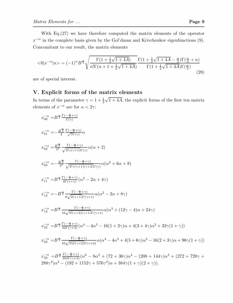
With Eq.(27) we have therefore computed the matrix elements of the operator
x−α in the complete basis given by the Gol’dman and Krivchenkov eigenfunctions (9).
Concomitant to our result, the matrix elements
<0|x−α|n> = (−1)nBα4
√
Γ(1 + 12
√1 + 4A)
n!Γ(n+ 1 + 12
√1 + 4A)
Γ(1 + 12
√1 + 4A− α
2 )Γ(α2 + n)
Γ(1 + 12
√1 + 4A)Γ(α
2 )(28)
are of special interest.
V. Explicit forms of the matrix elements
In terms of the parameter γ = 1 + 12
√1 + 4A, the explicit forms of the first ten matrix
elements of x−α are for α < 2γ:
x−α00 =B
α4
Γ(−α2+γ)
Γ(γ)
x−α01 =−B
α4
2
Γ(−α2+γ)√
γΓ(γ) α
x−α02 =B
α4
22
Γ(−α2+γ)√
2!γ(γ+1)Γ(γ)α(α+ 2)
x−α03 =−B
α4
23
Γ(−α2+γ)√
3!γ(γ+1)(γ+2)Γ(γ)α(α2 + 6α+ 8)
x−α11 =B
α4
Γ(−α2+γ)
4Γ(γ+1) (α2 − 2α+ 4γ)
x−α12 =−B α
4Γ(−α
2+γ)
8√
2(γ+1)Γ(γ+1)α(α2 − 2α+ 8γ)
x−α13 =B
α4
Γ(−α2+γ)
16√
3!(γ+2)(γ+1)Γ(γ+1)α(α3 + (12γ − 4)α+ 24γ)
x−α22 =B
α4
Γ(−α2+γ)
32Γ(γ+2) (α4 − 4α3 − 16(1 + 2γ)α+ 4(3 + 4γ)α2 + 32γ(1 + γ))
x−α23 =B
α4
Γ(−α2+γ)
32√
3!2!(γ+2)Γ(γ+2)α(α4 − 4α3 + 4(5 + 6γ)α2 − 16(2 + 3γ)α+ 96γ(1 + γ))
x−α33 =B
α4
Γ(−α2+γ)
384Γ(γ+3)(α6 − 8α5 + (72 + 36γ)α4 − (208 + 144γ)α3 + (272 + 720γ +
288γ2)α2 − (192 + 1152γ + 576γ2)α+ 384γ(1 + γ)(2 + γ)).

Matrix Elements for . . . Page 10
These matrix elements can be compared for the special case (A,B) = (0, 1) with the
matrix elements computed by the simple harmonic oscillator representation supple-
mented by Dirichlet boundary condition [1]. We have found an error in the value of
the matrix element x−α33 as given by [1]; this error is confirmed by a re-computation
according to the matrix element expression given by them. Indeed, the matrix element
x−α33 should read:
x−α33 =
Γ( 3−α2
)
7!Γ( 32 )
(α6 − 6α5 + 106α4 − 384α3 + 2080α2 − 3408α+ 5040)
instead of
x−α33 =
Γ( 3−α2 )
7!Γ( 32)
(α6 − 6α5 + 106α4 − 454α3 + 1660α2 − 3968α+ 5040)
as quoted by Aguilera-Navarro et al1.
In this work we have proved that the Gol’dman-Krivchenkov wavefunctions con-
stitute an orthonormal basis for the Hilbert space L2(0,∞). Using this orthonormal
basis, we are able to construct the matrix elements of x−α: the general result (Eq.27)
is convenient for use in any practical application which involves such singular potential
terms. It is also interesting that, with minor changes8, essentially involving only the
value of the coefficient A, the same formulas apply immediately to the corresponding
problems with non-zero angular momentum and in arbitrary spatial dimension N ≥ 2.
A detailed variational analysis of the spiked harmonic Hamiltonian operator based on
these matrix elements is presently in progress.
Acknowledgment
Partial financial support of this work under Grant No. GP3438 from the Natural
Sciences and Engineering Research Council of Canada is gratefully acknowledged.
References
1V. C. Aguilera-Navarro, G.A. Estevez and R. Guardiola. J. Math. Phys. 31, 99-104
(1990).
2I. I. Gol’dman and D. V. Krivchenkov, Problems in Quantum mechanics (Pergamon,
London, 1961).
Matrix Elements for . . . Page 11
3L. J. Slater, Confluent Hypergeometric Functions (At the University Press, Cambridge,
1960); F. W. Schafke, Einfuhrung in die Theorie der Speziellen Funktionen der Math-
ematischen Physik (Springer-Verlag, Berlin, 1963) Satz 1, p.162.4L. D. Landau and M. E. Lifshitz, Quantum Mechanics: Non-relativitic theory (Perg-
amon, Oxford, 1977).5W. Rudin, Real and Complex Analysis, 3rd (McGraw-Hill, New York, 1987) Theorem
1.3.4, p.26; Fubini-Tonelli theorem is discussed in p.164-166.6D. V. Widder, The Laplace Transform (Princeton University Press, Princeton, 1972)
Corollary 9.3b, p. 80; G. Doetsch, Handbuch der Laplace Transformation (Band I)
(Basel, Birkhauser, 1971) Satz 4, p.74.7H. Behnke and F. Sommer,Theorie der Analytischen Funktionen einer Komplexen
Veranderlichen (Springer-Verlag, Berlin, 1976) Satz 28, p.138.8R. L. Hall and N. Saad, J. Chem. Phys. 109, 2983-2986 (1998)

Matrix Elements for . . . Page 12
C’
t = 1t = 0
Im
Re
t-plane
Figure 1 The Contour C′ in the t-plane starting at 1 and enclosing the line segment
from 0 to 1.