
1
Linear Approximation

2
Outline
Review of Linear Approximation for Nonlinear Terms
A Case Study Renewable Sensor Networks with Wireless
Energy Transfer

Linear Approximation Motivation
Nonlinear optimization is difficult Linear programming is easy to solve with many
efficient tools available
Basic idea: Replacing nonlinear terms by some linear approximation approach Demonstrating piecewise linear approximation in this
chapter
3

Separable Problem
4
Objective function and constraint functions are additively separable
Constraint functions are linear and are constants

Piecewise Linear Approximation
: A continuous nonlinear function : A linear approximation of
5
(·)
(·)
𝜃(𝜇)
𝜇0=𝑎 𝜇1 𝜇𝑘− 1 𝜇𝑘𝜇𝜇2

General math expression for
: Weight for each grid point
Only two continuous and can be positive
All other must be zero
is defined as
6
Piecewise Linear Approximation (cont’d)

: A binary variable indicates whether falls within
the k-th segment
Relationship between and
7
Piecewise Linear Approximation (cont’d)

Back to the separable problem
Replacing each nonlinear function and by
its piecewise linear approximation
The solution to the linear approximating problem may or may not be feasible to the original separable problem Feasible: Accuracy/complexity vs. number of grid points
Infeasible: Construct a feasible solution by local search
8
Piecewise Linear Approximation (cont’d)

9
Outline
Review of Linear Approximation for Nonlinear Terms
A Case Study Renewable Sensor Networks with Wireless
Energy Transfer
Wireless Sensor Networks (WSNs)
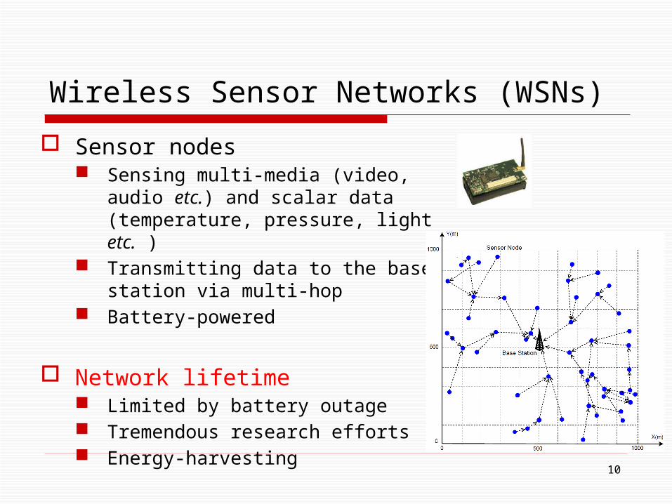
Sensor nodes Sensing multi-media (video, audio
etc.) and scalar data (temperature, pressure, light etc. )
Transmitting data to the base station via multi-hop
Battery-powered
Network lifetime Limited by battery outage Tremendous research efforts Energy-harvesting
10

WSNs (cont’d)
But lifetime remains a major performance bottleneck
Our objective Remove the fundamental performance bottleneck Motivated by the recent breakthrough in wireless
energy transfer
11

Wireless Energy Transfer
Dated back to the early 1900s by Nikola Tesla
Radiative mode by omni-directional antennas Low efficiency Never put into practice use
12

Wireless Energy Transfer (cont’d)
Little progress over nearly a century In early 1990, the critical need of wireless power transfer re-emerged
Example: electric toothbrush
Limited applications due to stringent requirements
Omni-directional antennas: close in contact Uni-directional antennas: accurate alignment in charging
direction, uninterrupted line of sight
13
Wireless Energy Transfer (cont’d)
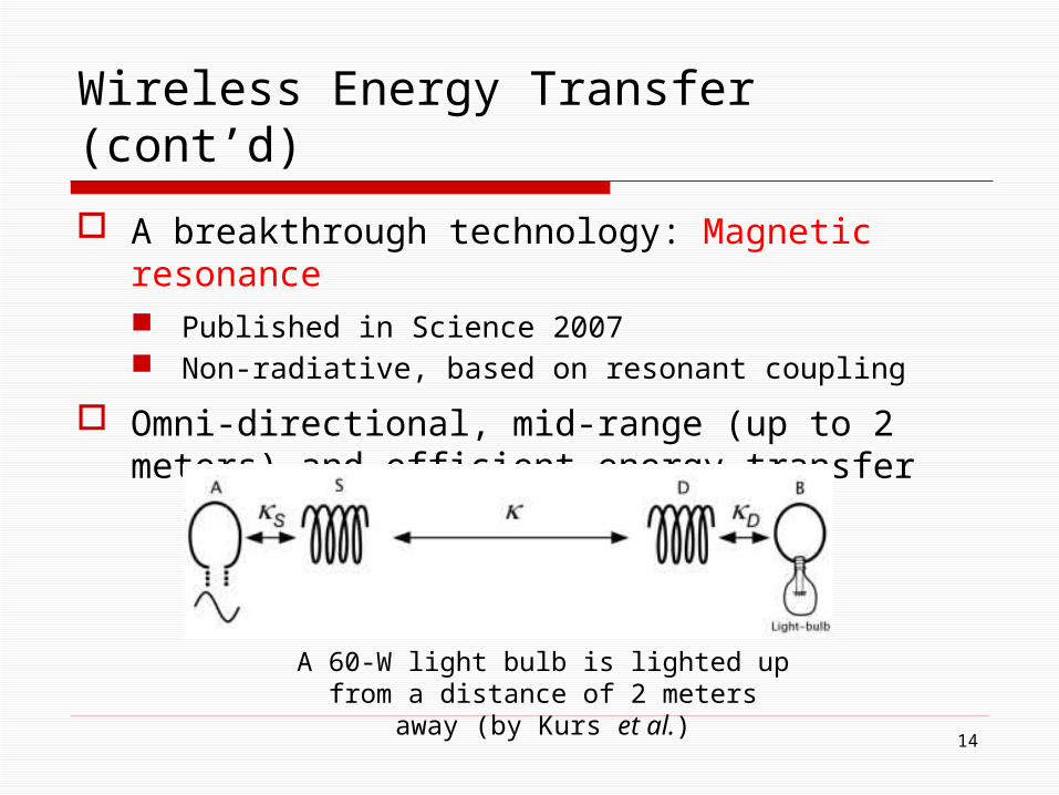
A breakthrough technology: Magnetic resonance Published in Science 2007 Non-radiative, based on resonant coupling
Omni-directional, mid-range (up to 2 meters) and efficient energy transfer
A 60-W light bulb is lighted up from a distance of 2 meters away (by Kurs et al.)
14
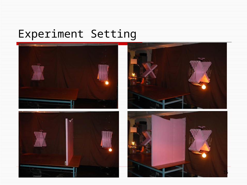
Experiment Setting
15

The emerging technology comes to reality!
Demonstrated in 2009 TED Global
The first No-tail TV was released at 2010 International CES
Wireless power consortium is setting the international standard for interoperable wireless charging
Revolutionize how energy is exchanged in the near future!
Wireless Energy Transfer (cont’d)
16

Problem Description
Objective:
1) Make sensor network work forever
2) Maximize the percentage of vacation time
Base Station
Sensor Node
Mobile Wireless Charging Vehicle (WCV)
Service Station
17

Three Basic Components
Traveling path (including direction) for WCV
Charging schedule at each node
Multi-hop data routing
18
19
Outline of Case Study A Solution Procedure
Renewable energy cycle
The optimal traveling path for WCV
The optimal charging schedule and multi-hop data routing
Numerical Results

Renewable Energy Cycle
i
Arrival time
Departure time
Vacation Time
Sensor Energy Behavior
Two requirements for renewable energy cycle are:1. Starts and ends at the same energy
level over a period of cycle. 2. Energy level never falls below
20
Optimal Traveling Path
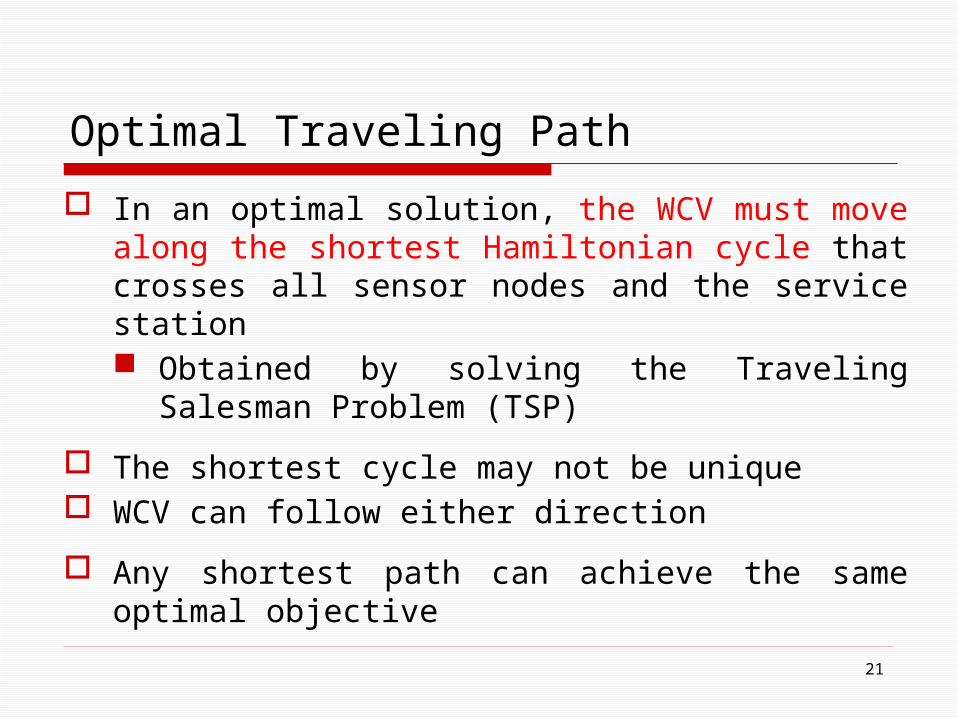
In an optimal solution, the WCV must move along the shortest Hamiltonian cycle that crosses all sensor nodes and the service station Obtained by solving the Traveling Salesman
Problem (TSP)
The shortest cycle may not be unique WCV can follow either direction
Any shortest path can achieve the same optimal objective
21

Charging Schedule and Data Routing
Traveling path for WCV
Charging schedule at each nodeMulti-hop data routing
22

Optimization Problem
The ratio of the WCV’s vacation time to a cycle time
Data routing
Charging schedule
Nonlinear optimization problem: NP-hard in general.
Consumed energy
23
Routing constraint
Energy consumption
Time constraint
Cycle constraints
A Near-Optimal Solution
24
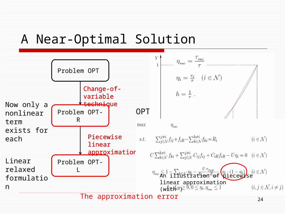
OPT-R
Problem OPT
Problem OPT-R
Problem OPT-L
Change-of-variable technique
Piecewise linear approximationPiecewise linear approximation
Now only a nonlinear term exists for each
An illustration of piecewise linear approximation (with )
The approximation error
Change-of-variable technique
Linear relaxed formulation

Performance Gap vs. Segment Number
Unknown optimal objective value of problem OPT
An upper bound is obtained by linear relaxation OPT-L
UB
LB A lower bound is obtained by feasible solution construction
Performance gap
Estimatedperformance
gap
Estimated performance gap is a decreasing function of m (the number of segments in approximation)
25

Unknown optimal objective value
An upper bound by linear relaxation
A feasible solution is constructed
UB
LB
3) Construct a provable near-optimal solution
Estimatedperformance
gap < є
Targetperformance
gap є
Choosing Segment Number
1) Given an arbitrarily small performance gap
2) Choose an appropriate (a function of )
26

Traveling path for WCV
Charging schedule at each node
Multi-hop data routing
The performance gap is no more than requirement є
Summary of Solution Approach
27

Sensor Energy Behavior- Complete Process
1st renewable energy cycle
The first renewable energy cycle starts.
2nd renewable energy cycle
Initial transient cycle
The first renewable energy cycle ends, i.e.,the second renewable
energy cycle starts.
0
28
29
Outline of Case Study A Solution Procedure
Renewable energy cycle
The optimal traveling path for WCV
The optimal charging schedule and multi-hop data routing
Numerical Results

A 50-node Network
Optimal traveling path Charging schedule
= 0.01m = 4
Cycle time = 30.73 hoursVacation time = 26.82 hoursPercentage = 87.27%
30

Results under Different Directions
Identical charging schedule and flow routing
Different arrival time and renewable cycle starting energy
31

Bottleneck Node
Provably show the existence of at least one “bottleneck” node in an optimal solution
32
Bottleneck node

Bottleneck Node (cont’d)
The energy behavior of the bottleneck node
33
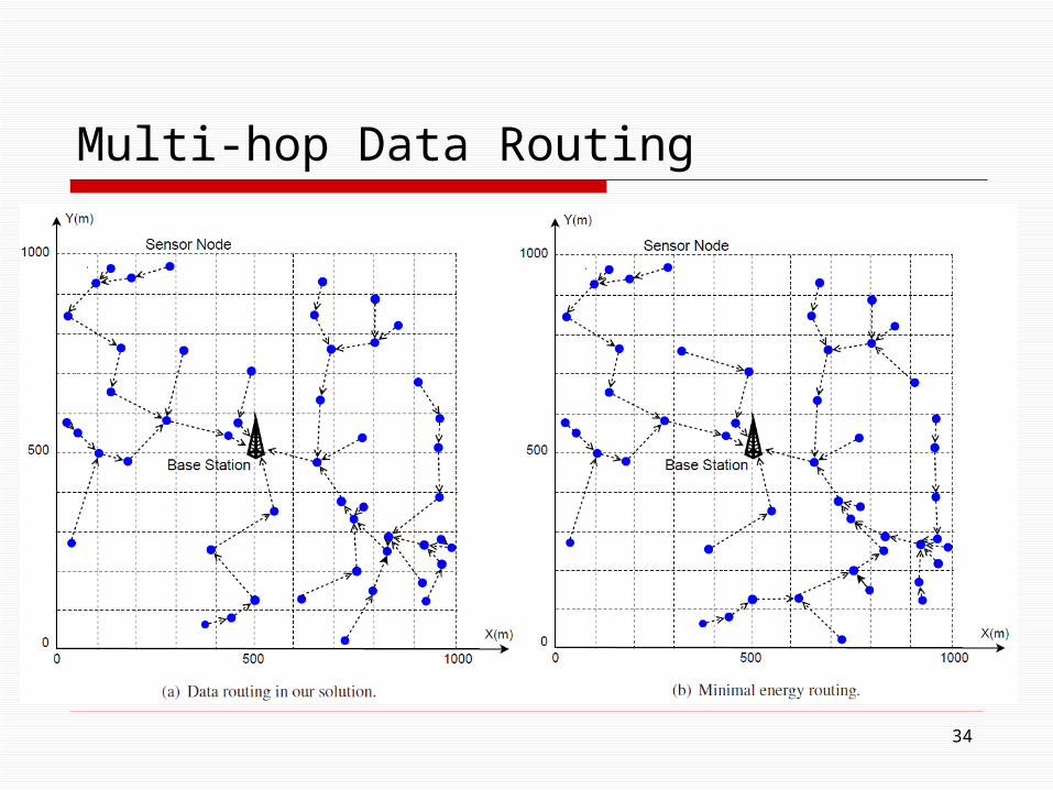
Multi-hop Data Routing
34
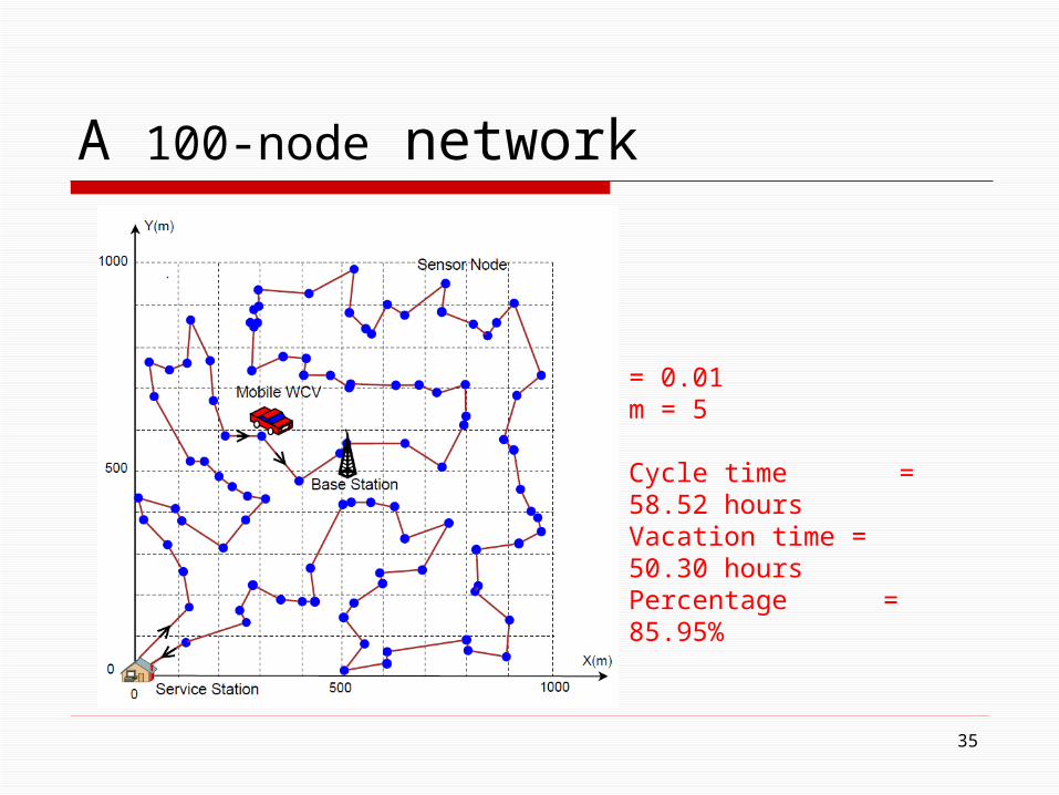
A 100-node network
35
= 0.01m = 5
Cycle time = 58.52 hoursVacation time = 50.30 hoursPercentage = 85.95%

Summary
36
Review of Linear Approximation for Nonlinear Terms
A case study Exploited recent breakthrough in wireless energy
transfer technology for a WSN Showed that a WSN can remain operational forever! Studied a practical optimization problem
Objective: Maximizing the ratio of the WCV’s vacation time over the cycle time
Proved that the optimal traveling path is the shortest Hamiltonian cycle
Developed a provable near-optimal solution for both charging schedule and flow routing