i
Land and Ecosystem Condition and
Capacity
DRAFT
Author: Michael Bordt1
Version: 1.0 (21 January 2015)
This work was undertaken as part of the project Advancing the SEEA Experimental Ecosystem
Accounting. This note is part of a series of technical notes, developed as an input to the SEEA
Experimental Ecosystem Accounting Technical Guidance. The project is led by the United Nations
Statistics Division in collaboration with United Nations Environment Programme through its The
Economics of Ecosystems and Biodiversity Office, and the Secretariat of the Convention on
Biological Diversity. It is funded by the Norwegian Ministry of Foreign Affairs.
1The views and opinions expressed in this report are those of the author and do not necessarily reflect the
official policy or position of the United Nations or the Government of Norway.

i
Acknowledgements: The author would like to thank the project coordinators (UNSD, UNEP and
the CBD), sponsor (the Norwegian Ministry of Foreign Affairs) and the reviewers, who contributed
valuable insights.

ii
0.1 Table of contents
1. Introduction .................................................................................................................................... 1
2. Links to SEEA-CF and SEEA-EEA ............................................................................................. 1 2.1 Discussion on links to EEA and how this guidance material is dealing with a particular issue ...... 1 2.2 Why is this important? ..................................................................................................................... 1
Ecosystem condition ........................................................................................................................................ 2 Ecosystem capacity ......................................................................................................................................... 2 Ecosystem characteristics (components) ......................................................................................................... 3
2.3 What is the issue being addressed? .................................................................................................. 3
3. Scope ............................................................................................................................................... 3 3.1 What is in and why? ......................................................................................................................... 3 3.2 What is out and why? ....................................................................................................................... 4
4. Discussion ....................................................................................................................................... 4 4.1 The Ecosystem Condition Account ................................................................................................. 4
Indicators of condition of characteristics ........................................................................................................ 5 Additional characteristics ............................................................................................................................... 9 Additional examples of measuring ecosystem condition ............................................................................... 14 Recommendations .......................................................................................................................................... 17
4.2 Accounting for changes in condition ............................................................................................. 18 4.3 Linking condition with capacity .................................................................................................... 19
Could convergence in scientific paradigms improve the linkages between conditions and capacity? .......... 19 Complexity, non-linearity and reductionism vs holism ................................................................................. 22 Approaches to addressing complexity ........................................................................................................... 26
4.4 Amenability to official statistics .................................................................................................... 27
5. Further work ................................................................................................................................ 28
6. Links to further material ............................................................................................................. 28
7. References ..................................................................................................................................... 29
8. Annex 1 Summary of suggested Condition Account measures for testing ............................. 35

1
1. Introduction
1. This report has been prepared as part of a project on Advancing Natural Capital Accounting2
through testing of the System of Environmental-Economic Accounting (SEEA) Experimental
Ecosystem Accounting. The objective of the report is to review the emerging concepts for
measuring ecosystem condition and capacity. It does so in the context of the SEEA Experimental
Ecosystem Accounting (SEEA-EEA) (European Commission, OECD et al. 2013).
2. Links to SEEA-CF and SEEA-EEA
2.1 Discussion on links to EEA and how this guidance material is dealing with a particular issue
2. The SEEA-EEA presents a broad, coherent and integrated measurement framework for linking
ecosystem extent, condition, capacity, services and values. Much knowledge and data exist
individually on each of these topics. However, bringing it into an integrated framework both
assures consistency in concepts and classifications and provides links to economic accounting.
3. To bring these concepts into an accounting framework, the SEEA-EEA defines several types of
accounts. These include spatially detailed, coherent and integrated information on ecosystems
(Asset Accounts), their condition (Condition Accounts) and the flow of services from them
(Production Accounts). Supporting this core are Carbon Accounts (including biocarbon), Water
Accounts (including quality), Biodiversity Accounts and the supply and use of ecosystem services
(Supply-Use Accounts).
4. With this in mind, the SEEA-EEA provides some initial principles and concepts in terms of
ecosystem condition and capacity. Taking these as a point of departure, this report reviews recent
literature to provide an overview of approaches used and to suggest means of further detailing the
SEEA-EEA concepts and, perhaps expanding them to be more generally applicable.
5. This report presumes the reader has a working knowledge of the SEEA-EEA. Training modules
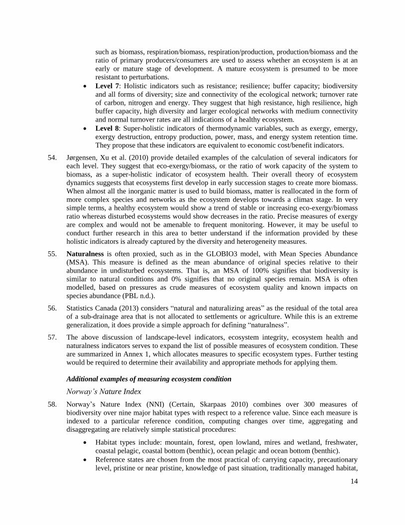
have been prepared as part of this project.
2.2 Why is this important?
6. For any multi-disciplinary research-oriented initiative, it is essential to establish a common sense of
existing concepts, measures, data and tools, but also to track the emerging ones. The SEEA-EEA
research agenda (p. 155) includes the following objectives related to the purpose of this report:
Identifying the main ecosystem characteristics for the measurement of ecosystem
condition and relevant indicators of condition for each type of ecosystem (e.g. forests,
wetlands, etc.) This work should consider the links to spatial units delineation.
Considering the links between expected flows of ecosystem services and measures of
ecosystem condition and extent, including assessment of relevant models and the
connections to issues such as resilience and thresholds. This work should also advance
understanding of ecosystem degradation in physical terms.
Investigating different approaches to determining reference conditions for the
assessment of ecosystem condition based on practical experience in countries.
7. This report will identify some opportunities for advancing these objectives in the research agenda
by testing of the SEEA-EEA.
2 See http://unstats.un.org/unsd/envaccounting/eea_project/default.asp.
2
Ecosystem condition
8. According to the SEEA-EEA, “Ecosystem condition reflects the overall quality of an ecosystem
asset, in terms of its characteristics.” (SEEA-EEA para 2.35). Note that the term “characteristics”
is used to specify ecosystem components (vegetation, biodiversity, soil, water and carbon).
9. Further, “Measures of ecosystem condition are generally combined with measures of ecosystem
extent to provide an overall measure of the state of an ecosystem asset. Ecosystem condition also
underpins the capacity of an ecosystem asset to generate ecosystem services and hence changes in
ecosystem condition will impact on expected ecosystem service flows.” (SEEA-EEA p. 164)
10. In addition, it suggests measuring ecosystem condition by choosing indicators representing the
quality of key components (such as water, soil, vegetation, biodiversity, carbon, nutrient flow,
connectivity and landscape configuration) with respect to a reference condition. (SEEA-EEA para
4.10-12)
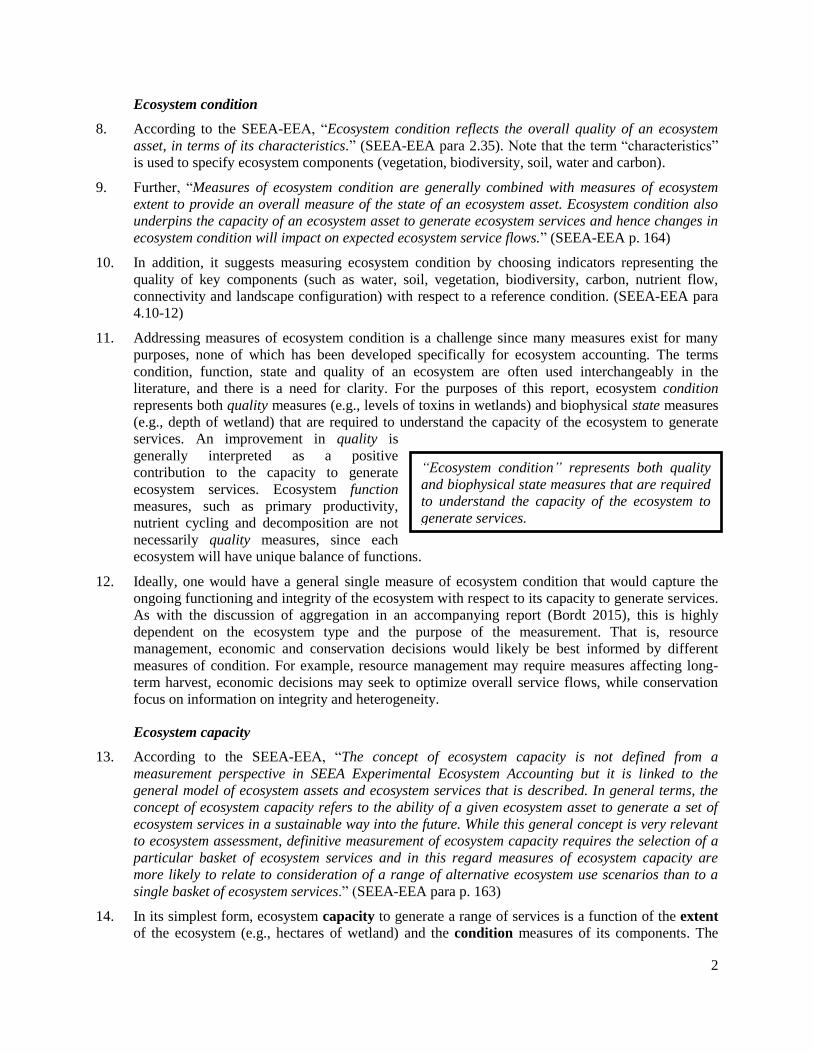
11. Addressing measures of ecosystem condition is a challenge since many measures exist for many
purposes, none of which has been developed specifically for ecosystem accounting. The terms
condition, function, state and quality of an ecosystem are often used interchangeably in the
literature, and there is a need for clarity. For the purposes of this report, ecosystem condition
represents both quality measures (e.g., levels of toxins in wetlands) and biophysical state measures
(e.g., depth of wetland) that are required to understand the capacity of the ecosystem to generate
services. An improvement in quality is
generally interpreted as a positive
contribution to the capacity to generate
ecosystem services. Ecosystem function
measures, such as primary productivity,
nutrient cycling and decomposition are not
necessarily quality measures, since each
ecosystem will have unique balance of functions.
12. Ideally, one would have a general single measure of ecosystem condition that would capture the
ongoing functioning and integrity of the ecosystem with respect to its capacity to generate services.
As with the discussion of aggregation in an accompanying report (Bordt 2015), this is highly
dependent on the ecosystem type and the purpose of the measurement. That is, resource
management, economic and conservation decisions would likely be best informed by different
measures of condition. For example, resource management may require measures affecting long-
term harvest, economic decisions may seek to optimize overall service flows, while conservation
focus on information on integrity and heterogeneity.
Ecosystem capacity
13. According to the SEEA-EEA, “The concept of ecosystem capacity is not defined from a
measurement perspective in SEEA Experimental Ecosystem Accounting but it is linked to the
general model of ecosystem assets and ecosystem services that is described. In general terms, the
concept of ecosystem capacity refers to the ability of a given ecosystem asset to generate a set of
ecosystem services in a sustainable way into the future. While this general concept is very relevant
to ecosystem assessment, definitive measurement of ecosystem capacity requires the selection of a
particular basket of ecosystem services and in this regard measures of ecosystem capacity are
more likely to relate to consideration of a range of alternative ecosystem use scenarios than to a
single basket of ecosystem services.” (SEEA-EEA para p. 163)
14. In its simplest form, ecosystem capacity to generate a range of services is a function of the extent
of the ecosystem (e.g., hectares of wetland) and the condition measures of its components. The
“Ecosystem condition” represents both quality
and biophysical state measures that are required
to understand the capacity of the ecosystem to
generate services.

3
main challenges here are selecting appropriate measures of condition for each component, and
addressing the complexity of ecosystem dynamics with respect to linking condition with capacity.
Ecosystem characteristics (components)
15. According to the SEEA-EEA, “Ecosystem characteristics relate to the ongoing operation of the
ecosystem and its location. Key characteristics of the operation of an ecosystem are its structure,
composition, processes and functions. Key characteristics of the location of an ecosystem are its
extent, configuration, landscape forms, and climate and associated seasonal patterns. Ecosystem
characteristics also relate strongly to biodiversity at a number of levels.
There is no classification of ecosystem characteristics since, while each characteristic may be
distinct, they are commonly overlapping. In some situations the use of the generic term
‘characteristics’ may seem to be more usefully replaced with terms such as ‘components’ or
‘aspects’. However, in describing the broader concept of an ecosystem, the use of the term
characteristics is intended to be able to encompass all of the various perspectives taken to describe
an ecosystem.” (SEEA-EEA p. 164)
16. As stated in the SEEA-EEA research agenda (quoted above), the challenge is to identify key
characteristics for each ecosystem type. For example, biomass production, when applied to a
freshwater ecosystem needs to be interpreted differently than for a terrestrial ecosystem; excess
biomass in freshwater implies, in many instances, the negative quality of eutrophication.
2.3 What is the issue being addressed?
17. This report addresses measures of ecosystem condition and capacity from an accounting
perspective. It begins with a review of how these issues are represented in the SEEA-EEA and
suggests how testing in the areas of incompleteness (which characteristics and which measures of
those characteristics) may be informed by emerging work in the scientific literature and ecosystem
accounting activities. Focussing on the SEEA-EEA Table 4.3 as the starting point for defining a
Condition Account, it also suggests linkages with other SEEA-EEA accounts:
the Asset Account (for recording the stock of ecosystem types and changes in their
stocks),
the Biodiversity Account (for recording species-specific or habitat-specific information
not easily aggregated into the Condition Account)
the Water Account (for recording the stock, flow and quality of water) and
the Carbon Account (for recording carbon stocks and flows, including biocarbon, which
is often an indicator of ecosystem condition).
3. Scope
3.1 What is in and why?
18. This report focuses on expanding the scope of the SEEA-EEA for future testing of the Condition
Account. Based on extensive literature review and examples of application, it suggests additional
measures for the existing characteristics defined in SEEA-EEA Table 4.3. It also suggests
additional characteristics, including measures of integrity and heterogeneity.
19. This report also reviews the scientific basis for linking ecosystem conditions with capacity to
generate services. This is challenging and controversial for many reasons, not only due to the
complexity of ecosystems, but also to the varying viewpoints among scientists and users.

4
20. We suggest that, in testing the SEEA-EEA,
these challenges and controversies be
addressed by the development of specific
tools to codify and integrate existing
knowledge in the area.
21. Finally, this report recommends a role for
National Statistical Offices in compiling
this information and in developing these tools.
3.2 What is out and why?
22. This report does not provide detail on the construction or compilation of specific measures. For
example, the calculation of an ecosystem’s exergy is provided in textbooks. Although some
ecosystem-specific measures are addressed, there is much research that could better be incorporated
into a compilation manual after initial testing is completed.
23. Many models exist that link specific ecosystem conditions with their capacity to generate services.
These are based on known ecological relationships and incorporate various assumptions about how
these relationships result in the flow of ecosystem services. These models are not discussed in this
report, but some aspects are summarized in an accompanying report (Bordt 2015).
24. The SEEA-EEA recommends combining condition measures into an index. Some advice on
creating such an index is provided in an accompanying report (Bordt 2015).
4. Discussion
4.1 The Ecosystem Condition Account
25. This section begins with a description of the current recommendations in the SEEA-EEA in terms
of ecosystem condition and suggests additional measures that may be available to augment the
indicators suggested for each ecosystem characteristic. It then suggests additional characteristics
that could be tested for inclusion in a Condition Account. The section then reviews some of the
applications of ecosystem condition measures and suggests approaches to establishing a more
comprehensive Condition Account.
26. Table 4.3 in the SEEA-EEA document (Figure 1) provides a starting point for defining a Condition
Figure 1 Ecosystem condition as represented by the SEEA-EEA
Linking ecosystem condition with capacity to
generate services is challenging and
controversial due to the complexity of
ecosystems and to the varying viewpoints among
scientists and users.

5
Account. For each ecosystem type (or
LCEU type), each characteristic is
attributed with a proposed set of measures
of condition. Some of these condition
indicators indicate quality, while others
reflect biophysical state parameters that are
not directly associated with quality (such as
river flow).
27. Dividing an LCEU type into characteristics (or components) focusses the selection of indicators
into standard measures (that is, water quality, soil quality, species diversity…). Although intended
mainly as a starting point, the current concept of a Condition Account would benefit from (a) being
more precise about the actual indicators suggested, and (b) expanding the list of components to
include a wider range of measures that operate across characteristics, such as those related to
ecosystem integrity.
Indicators of condition of characteristics
28. The selection of indicators will largely be
driven by availability. However, it is
essential that at least a core set of condition
indicators be attributed to each LCEU
characteristic. Without condition indicators,
there is no means to assess changes in those conditions or link the ecosystem asset with its capacity
to generate services.
29. In terms of vegetation, some aspects of its condition would be captured in other characteristics,
such as the diversity of species. The indicators suggested are leaf area index (LAI), mean annual
increment, and biomass:
According to Carlson and Ripley (1997), LAI is physical property of the vegetation
canopy and is closely related to NDVI (normalized difference vegetation index, a
standard remotely sensed vegetation index), vegetation condition and biomass.
Mean annual increment (MAI) normally refers to the increase in the growth of trees, or
a stand of trees, in terms of diameter and or height (Piotto 2008).
Biomass (indicating productivity, and to some degree the health of a terrestrial
ecosystem) is most easily be measured in terms of above ground biomass, which can be
estimated from remotely sensed NDVI (Hansen, Schjoerring 2003). In some ecosystems,
such as prairie grasslands, below-ground biomass can exceed that above ground.
Measuring below-ground biomass would require estimation from known species
distributions, field samples or laboratory studies.
30. While these measures may be appropriate for vegetation in many terrestrial ecosystems (forests,
shrublands and grasslands), additional measures may be required for vegetation in wetlands,
freshwater, coastal and marine ecosystems:
For wetlands, general measures of vegetation condition suggested by Fennessy, Jacobs et
al. (2004) include the number of vegetation classes and the extent of invasive species.
Approaches to assessing freshwater, coastal and marine ecosystems generally assess the
nature of the vegetation, rather than overall biomass production, as an input to
assessments of naturalness or disturbance. For Dennison, Orth et al. (1993) assess water
quality in terms of the submersed aquatic vegetation species. In this respect, the condition
It is essential that a core set of condition
indicators be attributed to each LCEU
characteristic.
A Condition Account would benefit from (a)
being more precise about the actual indicators
suggested, and (b) expanding the list of
components to include a wider range of
measures that operate across characteristics,
such as those related to ecosystem integrity.

6
of vegetation in these ecosystems could also include the number of vegetation classes and
the extent of invasive species.
31. The condition indicators suggested in the SEEA-EEA for the characteristic biodiversity are:
Species richness is a simple count of the number of species living in a given ecosystem.
This measure says little about the diversity of species since endemic, rare, common and
invasive species are all counted with equal weight.
Relative species abundance is a measure of the number of individuals in given species
relative to those in other species, usually within the same trophic level. In most
ecosystems, there are more rare species than common ones. This may be useful to
indicate whether or not an ecosystem is diverging from an equilibrium state (See Volkov,
Banavar et al. 2003 for a discussion).
32. Besides species richness and abundance, it may also be useful to measure the diversity of species
using a standard index such as the Shannon Diversity Index. Although the linkages are not linear,
there is abundant evidence that diversity contributes to ecosystem function and resilience
(Cardinale, Duffy et al. 2012).
33. The Biodiversity Indicators Partnership suggests the following indicators of the state of
biodiversity:
Red list index “measures the overall rate at which species move through IUCN Red List
categories towards or away from extinction. It is calculated from the number of species
in each category (Least Concern, Near Threatened, Vulnerable, Endangered, Critically
Endangered, Extinct), and the number changing categories between assessments as a
result of genuine improvement or deterioration in status (category changes owing to
improved knowledge or revised taxonomy are excluded). Tracking the net movement of
species through the Red List categories provides a useful metric of changing biodiversity
status.” This could be included as an indicator of ecosystem condition in the Condition
Account.
Extent of forest & forest types is “measured as the proportion of land area under
forests”. In terms of ecosystem accounts, this would be captured in the Asset Account.
Extent of marine habitats tracks the extent of mangroves, seagrass beds and coral reefs
and, as such, would also be captured in the Asset Account.
Area of forest under sustainable management should also be captured in the Asset
Account, if management regime is included in the criteria used to delineate LCEUs.
Otherwise, it could be included in the Condition Account.
Forest fragmentation, indeed any ecosystem fragmentation measure could be captured
in the ecosystem Condition Account at a higher level than LCEU. If the linear features
that cause fragmentation (e.g., roads, railways, pipelines, electrical infrastructure) are
used to delineate LCEUs, then the measure of fragmentation would need to apply at the
EAU or groups of LCEUs of similar type within an EAU.
River fragmentation and flow regulation measures the proportion of rivers with dams.
As with forest fragmentation, this would need to be applied to an EAU or groups of
LCEUs in the Condition Account.
Ex-situ crop collections tracks the number genetic samples of economically valuable
crops and animals and their wild relatives that have been collected. This may apply to
agricultural LCEUs with unrecorded agricultural species and their relatives. This could be
recorded in the Biodiversity Account.

7
Genetic diversity of terrestrial domesticated animals measures the number of
domesticated breeds that are locally adapted or exotic. In ecosystem accounting, this may
be applicable to agricultural ecosystems and be recorded in the Biodiversity Account.
The Wildlife Picture Index “aggregates biodiversity camera trap data for ~300 species
of tropical terrestrial mammals and birds to assess species trends and extinction risks”.
This could be a useful management indicator in the Biodiversity Account for areas in
which these species are monitored.
VITEK is an “indicator for assessing the vitality of traditional environmental knowledge
(TEK) across generations within a given community or population. Vitality is defined as
the rate of retention of knowledge over a specified time period. The inverse of the
retention value is effectively the amount and speed of TEK change.” For ecosystem
accounting, this may be an appropriate indicator of management within socio-ecological
systems, but not necessarily specific LCEU types. This may be best captured in a
Biodiversity Account.
34. Measures may be available on specific species condition (e.g., toxics in tissues, incidence of
disease, reproduction rates, age distributions, indicator species, keystone species, functional and
response diversity), but these may be more appropriate for a separate Biodiversity Account.
35. The condition indicators suggested in the SEEA-EEA with respect to soil include:
Soil organic matter content: Soils are either organic (more than 20% carbon content) or
mineral-based (less than 20% carbon content). According to (Burke, Yonker et al. 1989),
soil carbon is a major source of system stability in agricultural ecosystems and it changes
with respect to the texture of the soil and amount of rainfall.
Soil carbon (or organic carbon stock) measures the content of soil carbon. This, for most
purposes is the same measure as soil organic matter content. This may be linked with the
SEEA-EEA Carbon Account.
Groundwater table is a measure of the depth to the groundwater table or aquifer. The
groundwater table can rise and fall in response to changes in rainfall and intensive
irrigation for agriculture. According to the FAO (2003), the impacts of over-abstraction
and aquifer degradation by pollution have been reported widely, not only to the local
users of the groundwater for purposes such as irrigation, but also to downstream
communities that are also dependent on the resource.
36. Other available measures of soil condition could include soil class (Bordt 2013), soil moisture
content, topsoil texture and degree of erosion. Toxic substances that accumulate in soil and
streambeds may also be monitored and could be included in this characteristic. For coastal water
bodies, rates of coastal erosion could be important to monitor if there are concerns of land area lost
due to the loss or degradation of protective infrastructure such as mangroves or coral reefs.
37. The condition indicators suggested in the SEEA-EEA with respect to water include:
River flow rate: This is a relative indicator (such as m3/second) in that flow rates with
change over the seasons and between years of relative drought and flooding. What is
likely more important to track is the fluctuation or variability in flow and how these
fluctuations vary over time. Statistics Canada (2010) showed that areas of the country,
especially where intensive agriculture is taking place are increasingly at risk of both
flooding and drought. This may be applied to wetlands as well in that the flow rate (or
Hydrological Retention Time, HRT) is an important indicator of ecosystem function in
terms of its capacity to remove pollutants (Akratos, Tsihrintzis 2007).
Water quality: Hundreds of water quality parameters are measured regularly to monitor
the quality of surface waters, intakes to water treatment plants and groundwater. Each

8
parameter is normally associated with a “standard” or level of this parameter that should
not be exceeded for a specific purpose, such as livestock watering, irrigation, swimming
or drinking. Common measures include biochemical oxygen demand (BOD), chemical
oxygen demand (COD), pH, turbidity, total suspended solids (TSP), temperature,
nutrients (nitrogen and phosphorous), toxics (such as mercury, lead, PCBs, pesticides and
cadmium). It is important to note that monitoring of water quality often focuses on areas
of concern and therefore parameters are selected to represent a specific human pressure
(e.g., agriculture, municipal runoff, industrial wastewater discharge). To combine several
parameters into a single index, some jurisdictions, such as Canada, use an index based on
the number of parameters that exceed their specific allowable levels (Environment
Canada, Statistics Canada & Health Canada 2007).
Fish species: Although fish should be included in the Condition Accounts (Biodiversity
Characteristic) with respect to their abundance and diversity, freshwater and marine fish
species also serve as a reflection of the quality of the aquatic ecosystem. Since tissues
tend to accumulate toxins (such as mercury), measures of chemical residues in fish may
also be used as indicators of freshwater ecosystem condition.
38. Additional indicators of condition of water could include:
Inland Waters Bodies and Open Wetlands: variability of streamflow (historical and
recent)
Coastal Water Bodies and Sea: Wave intensity (historical and current)
Open Wetlands: Hydrological Retention Time (HRT)
39. The condition indicators suggested in the SEEA-EEA with respect to carbon include:
Net carbon balance (or net ecosystem carbon balance) is a measure of the difference
between the amount of biomass produced in an ecosystem and the amount lost (e.g., by
fire or removal by humans). This should apply to all ecosystems in that removal from
soil, vegetation and animals reflects a decrease in carbon stocks available to the
ecosystem. This should be further explored in the guidance document on Carbon
Accounts.
Primary productivity is a measure of the rate at which atmospheric or aqueous CO2 is
converted to organic compounds. Clark, Brown et al. (2001) define Net Primary
Production (NPP) as the difference between total photosynthesis (Gross Primary
Production, or GPP) and total plant respiration in an ecosystem. They note that field
measurements are normally restricted to litter mass and aboveground biomass. However,
this ignores the belowground production. With respect to Net Carbon Balance, NPP
would represent the total biomass produced that would then be adjusted for
anthropocentric losses. Although this is a component of the Carbon Account, it is also a
measure of overall ecosystem condition.
40. Additional indicators of the condition in an ecosystem Carbon Account could include carbon loss
from respiration and metabolic efficiency in terms of respiration as a fraction of total biomass (see
below).
41. Marine and coastal ecosystems are not be well represented by the indicators of condition discussed
so far. Although biodiversity and water quality measures would apply, they are subject to issues
including, among others, acidification, sea level, wave action and coastal erosion (French,
Burningham 2013). Since coral reefs and mangroves mitigate the impacts of coastal erosion,
specific indicators of their status could be included in the Condition Account.
42. For most ecosystems, there is an optimal level for each of these indicators. For example,
eutrophication in a lake would show an increase in biomass. The introduction of invasive species

9
may show an increase in diversity. It is therefore essential to calibrate indicators of condition for
specific ecosystem types and with an optimal or ideal reference state. This is discussed further in an
accompanying report (Bordt 2015).
Additional characteristics
43. The most straightforward addition to Table 4.3 would be accounting for the quality of air. Air
quality measures are abundant and would give an additional indication of the condition of the
ecosystem. Standard air quality measures include: particulate matter (PM2.5 and PM10), nitrogen
oxides (NOx), sulfur dioxide (SO2), ground-level ozone (O3), carbon monoxide (CO) and rainwater
pH. Most air quality indices are designed for human health purposes. Canada’s Air Quality Index,
for example, combines ground level ozone, nitrogen dioxide and particulate matter (PM2.5 and
PM10) into a single index. According to Akimoto (2003), some of these measures can be obtained
from remote sensing information. Malouin, Doyle et al (2013) use modelled Nitrogen and Sulphur
deposition exceedances as a component of a wetland purification potential index.
44. Some measures of condition may be used in the delineation of the LCEUs and would therefore not
need to be captured separately in a Condition Account. These could include the slope, elevation,
land use intensity (of cropping and livestock grazing), management regime (protected, in
production) and location with respect to the drainage area (upper, middle or lower catchment).
Other general biophysical measures that could contribute to understanding ecosystem condition
include: average temperature, average rainfall, hours of sunlight/cloud, growing degree days,
proximity to humans and UV intensity.
Although these would not be expected to
change rapidly over time, such information
may be important to assessing longer-term
changes with respect to the capacity of the
ecosystem to generate services.
45. By focussing on components, the existing scheme of measuring ecosystem condition does not
account for aspects that operate across ecosystem types and across components. This would require
the use of landscape-level (that is, aggregates of adjacent LCEUs) measures and measures of
ecosystem integrity, health and naturalness.
46. Landscape-level indicators in the Condition Account would require the addition of measures such
as fragmentation, ecosystem diversity (structural and species complexity, patchiness), corridors,
buffers and gradients.
47. Fragmentation is a measure of the degree to which an ecosystem is divided into smaller areas by
human built infrastructures such as dams, roads, railways, pipelines and electrical infrastructure.
This is discussed above in terms of forest and river fragmentation, but applies to other ecosystem
types as well. It is also noted above that fragmentation measures would most likely apply to spatial
units larger than the LCEU since an LCEU is by definition an unfragmented land cover type.
Statistics Canada (2013) uses a measure of barrier density in terms of km of barriers per km2 of the
sub-drainage area.
48. Fischer, Lindenmayer et al. (2006) suggest ten principles for landscape management in commodity
production landscapes such as production forests and croplands. These principles apply as well to
managed natural landscapes such as protected areas and could serve as guidance on what measures
could indicate integrity. Like fragmentation, most of these measures would not be measured at the
LCEU level, but at a higher aggregate. These principles are:
Pattern-oriented management strategies:
Measures of air quality, heterogeneity and
holistic measures of ecosystem health,
naturalness and integrity would enhance the
Condition Account.

10
o Maintain and create large, structurally complex patches of native vegetation:
This implies measuring the patchiness of landscapes and the proportion of native (or
endemic) vegetation. Individual LCEUs could be designated as containing native
vegetation or not and the ratio of native to non-native vegetation could be monitored
over time.
o Maintain structural complexity throughout the landscape: Structural complexity
provides habitat for some native species, enhanced landscape connectivity, and
reduced edge effects. This also implies measuring the complexity or number of
distinct ecosystem types within a landscape.
o Create buffers around sensitive areas: As with structural complexity, buffers help
mitigate negative impacts on sensitive species. These buffers may be less pristine, but
provide regulation and maintenance services to the sensitive area. In terms of
measures at the LCEU level, LCEUs could be designated as sensitive area or buffer.
Whether or not sensitive areas had buffers would need to be determined with spatial
analysis. A simple metric might be the ratio of buffer to sensitive area at the EAU
level. This has been tested by Malouin, Doyle et al. (2013) in terms of the ratio of
riparian forest cover (in %) to the average linear density of rivers and streams (in %).
o Maintain or create corridors and stepping stones: Corridors are elongated strips of
vegetation that link patches of native vegetation; stepping stones are small patches of
vegetation scattered throughout the landscape. As with buffers, LCEUs could be
designated as corridors or stepping-stones. Similarly, a simple metric would be the
ratio of corridor or stepping-stones to larger patches of native vegetation.
o Maintain landscape heterogeneity and capture environmental gradients:
Landscapes that resemble natural patterns, even if they are used for agriculture and
forestry, provide more benefits than large areas of intensively managed
monocultures. Gradients refer to varying conditions of temperature, moisture or
primary productivity. Landscape heterogeneity, like structural complexity can be
measured in terms of the number of LCEU types within a given EAU. Gradients
could be measured in terms of the diversity of conditions.
Process-oriented management strategies:
o Maintain key species interactions and functional diversity: Species interactions
such as competition, predation and mutualistic associations can be maintained to
some degree by maintaining keystone species and maintaining species diversity
within functional groups. Keystone species are those which have a disproportionate
effect on ecosystem function (such as pollinators and seed transporters). Functional
diversity refers to different species that provide similar ecosystem functions such as
waste decomposition and predation. Measures of keystone species and functional
groups could be applied in the Biodiversity Account.
o Apply appropriate disturbance regimes: Ecosystems have evolved to depend on
natural disturbances such as fires, successional stages and grazing by large
herbivores. When these are altered by humans, irreversible changes in ecosystem
function may result. Fischer, Lindenmayer et al. (2006) suggest mirroring natural
disturbance regimes. For fires, this might be tracked in terms of the frequency,
intensity and spatial scale of fires in relation to what is considered natural for that
ecosystem. Malouin, Doyle et al. (2013) use the Canadian National Fire Database to
determine ecosystem-specific fire regimes with respect to the implications for water
purification potential.
o Control aggressive, over-abundant, and invasive species: Conditions that favour
tree and agricultural crops may favour the growth of aggressive native or exotic

11
species. Increases in their populations may further negatively impact the stability of
the landscape by increased competition or predation. This could be captured in the
Biodiversity Account by tracking the population levels of specific species.
o Minimize threatening ecosystem-specific processes: Additional threats, such as
hunting by humans and chemical pollution are situation specific. Chemical pollution
is already captured in the Condition Account as a property of the LCEU. Intensity of
hunting or other forms of poaching could be captured in terms of intensity of land
use.
o Maintain species of particular concern: Given the focus on diversity in general,
functional groups and resilience, it is also important to main specific species that may
contribute little to ecosystem function. These would include rare and threatened
species, but also species of cultural or local significance. These could also be
captured in the Biodiversity Account.
49. Indicators of ecosystem integrity, ecosystem health and naturalness include measures of conditions
both between ecosystem types and between components. Kandziora, Burkhard, et al. (2012)
suggest some measures of structural and functional integrity that reflect the capacity of ecosystems
to generate services. These overlap with some of the indicators already discussed, but are include
here in their entirety:
Exergy capture (the capacity of an ecosystem to enhance the input of useable energy) is
proxied with a measure of net primary productivity (NPP) and leaf area index (LAI). This
is already captured in the core SEEA-EEA Condition Account.
Entropy production (non-convertible energy fractions that are exported into the
environment of the system) is proxied with a measure of Carbon/year from respiration.
This could be considered for inclusion in the Carbon Account.
Storage capacity (the capacity of an ecosystem to store nutrients, energy and water when
available and to release them when needed) is proxied with a measure of organic carbon
and nitrogen in the soil. This could be included as an additional measure of soil in the
Condition Account.
Cycling and nutrient loss reduction (the capacity of an ecosystem to prevent the
irreversible output of elements from the system) is measured in terms of the degree of
leaching of nutrients such as nitrogen and phosphorous. This could be considered as an
additional measure of soil condition in the Condition Account.
Biotic water flows (water cycling affected by plant processes in the system) is measured
in terms of transpiration as a fraction of total evapotranspiration. This could be
considered as an additional indicator for the condition of vegetation in the Condition
Account.
Metabolic efficiency (The amount of energy necessary to maintain a specific biomass,
also serving as a stress indicator for the system) is measured in terms of respiration as a
fraction of total biomass (or the metabolic quotient). This may be considered as an
additional indicator in the Carbon Account.
Heterogeneity (The capacity of an ecosystem to provide suitable habitats for different
species, for functional groups of species and for processes) is measured in terms of the
heterogeneity of the abiotic components of the system (such as humus content of the soil)
and the number of habitats per area. This could be included in the summary of ecosystem
condition at a larger spatial scale (such as EAU) in terms of number of LCEU types.
Biotic diversity (the presence and absence of selected species, (functional) groups of
species, biotic habitat components or species composition) is measured in terms of
specific indicator species, the Shannon-Weiner Index and the Simpson Index. These
could be considered for inclusion in the Biodiversity Account.

12
50. Ecosystem health (Rapport, Costanza et al. 1998, Jørgensen, Xu et al. 2010) is based on the
premise that “healthy” ecosystems are more likely to be resilient, function optimally and provide an
ongoing flow of services. Although the metaphor to human health has been criticized, it is useful to
review the indicators suggested by this field.
51. Rapport (1998) suggests the following measures of ecosystem distress (the Ecosystem Distress
Syndrome, EDS), particularly for multiply-stressed aquatic and arid ecosystems:
System properties:
o Primary productivity (higher if stressed): As noted above, with respect to the
Carbon Account, this the rate at which atmospheric or aqueous CO2 is converted to
organic compounds.
o Horizontal nutrient transport (higher if stressed): This refers to the horizontal
distance to which nutrients are transported. In a healthy ecosystem nutrient flows
between biota and substrate dominate. This implies a reduced efficiency of nutrient
cycling (Rapport, Whitford 1999). For inland water ecosystems this may be measured
in terms of the distance from outfall that nutrients can be detected.
o Species diversity (lower if stressed): This is also discussed above in terms of the
Biodiversity Account.
o Disease prevalence (higher if stressed): This is species specific. It can be monitored
in terms of the frequency of tumors and parasites. This could be considered for
testing as part of the Biodiversity Account.
o Population regulation (lower if stressed): Although there are short-term and long-
term natural population cycles (Holling 1973), some stresses will lead to sharp
increases or decreases in the population of specific species. This could also be
considered for testing as part of the Biodiversity Account.
o Reversal of succession (higher if stressed): Succession is the change over time from
relatively simple, pioneer ecosystems to more complex climax ecosystems (Cox,
Moore 2010). A reversal of succession implies a regression back to simple
ecosystems than can exist in harsher conditions, such as soil that is poor in organic
matter. This phenomenon is already captured in other measures of diversity and
heterogeneity.
o Metastability (lower if stressed): With respect to ecosystems, this refers to “local
stability and resilience of dominant biotic communities”. Trends in species diversity,
species populations, age distributions and stage of succession could be indicators of
metastability in the Biodiversity Account.
Community properties:
o Proportion of r-selected species (higher if stressed): r-selected species are those
with a high potential rate of population increase. This is a characteristic of early
colonists of a succession (Cox, Moore 2010). K-selected species are slower to
reproduce, but are more able to sustain their population when close to the carrying
capacity. Tracking this ratio could be tested in the Biodiversity Account.
o Proportion of short-lived species (higher if stressed): This is similar to r-selected
species, since r-selected species also tend to be shorter lived.
o Proportion of smaller biota (higher if stressed): This is also related to the r-
selected/K-selected ratio, since r-selected species tend to be smaller.
o Proportion of exotic species (higher if stressed): Exotic, non-endemic species may
be a cause of the stress, or the stress may be opening niches in the ecosystem for
exotic species to exploit. This could be included for testing in the Biodiversity
Account.

13
o Mutualistic interactions between species (lower if stressed): As ecosystems
develop, interactions tend to become more complex. This can be shown in terms of
the complexity of the food web, which increases with increased species diversity
(Paine 1966).
o Boundary linearity (higher if stressed): Boundaries between ecosystem types (or
ecotones) can vary in thickness, continuity and linearity (Wiens, Stenseth et al.
1993). This can be taken to mean that stressed ecosystems tend to have distinct
boundaries. This may be captured in the Condition Account in terms of buffers.
o Extinction of habitat specialists (higher if stressed): As an ecosystem develops
from pioneer to climax, increasing diversity and complexity provide narrower niches
for species to exploit. Specialists tend to exploit one or a few similar habitats, while
generalists use a wide range of disparate habitats (McPeek 1996). Recording whether
a species is a specialist or generalist is suggested for the Biodiversity Account.
52. Most of the measures suggested by Rapport as indicators of ecosystem health have already been
discussed or could be considered for testing in a Biodiversity Account.
53. Jørgensen, Xu et al. (2010) classify ecosystem health indicators into eight levels, from the most
reductionist to the most holistic. This classification is illustrative of the hierarchy of indicators for
consideration in a Condition Account. Many examples are derived from freshwater ecology, but
could also be applicable to terrestrial, coastal and marine ecosystems:
Level 1: The presence or absence of specific species. This is often used when the
tolerance of certain species is known, such as the tolerance of fish species to certain
pollutants. Some species dominate in unpolluted water, others will dominate in polluted
water, whereas others may be indifferent.
Level 2: The ratio between classes of organisms. For example the Nygaard Algae Index,
which is a ratio of indicator algal groups, with higher values indicating a more eutrophic
condition (Sullivan, Carpenter 1982).
Level 3: Concentrations of chemical compounds in in water, soil, plant and animal tissue.
Examples are the assessment of eutrophication on the basis of total phosphorous
concentration. This would also include concentrations of toxics, such as PCBs in animal
tissue and water.
Level 4: Concentration of entire
trophic levels. For example, the
concentration of phytoplankton as
another indicator of eutrophication.
Optimal concentrations of bird or
fish species are also used as
indicators of healthy ecosystems.
Level 5: Process rates, such as
primary production. In freshwater
ecosystems, this is an indicator of
eutrophication. However, high
annual growth of trees in a forest
and of animal populations are used
as indicators of healthy
ecosystems. High mortality may be
used as indicators of unhealthy
ecosystems.
Level 6: Composite indicators
The Condition Account would benefit from a
hierarchy of condition indicators:
1. Most reductionist: presence or absence of
specific species
2. Ratios between classes of organisms
3. Concentration of chemical compounds
4. Concentration of species trophic levels
5. Process rates (e.g., primary production)
6. Composite indicators (biomass,
respiration/biomass, respiration/production)
7. Holistic indicators (resistance, resilience,
buffer capacity, diversity, size and
connectivity, turnover rate of carbon,
nitrogen and energy
8. Super holistic: thermodynamic variables
(exergy, emergy)
14
such as biomass, respiration/biomass, respiration/production, production/biomass and the
ratio of primary producers/consumers are used to assess whether an ecosystem is at an
early or mature stage of development. A mature ecosystem is presumed to be more
resistant to perturbations.
Level 7: Holistic indicators such as resistance; resilience; buffer capacity; biodiversity
and all forms of diversity; size and connectivity of the ecological network; turnover rate
of carbon, nitrogen and energy. They suggest that high resistance, high resilience, high
buffer capacity, high diversity and larger ecological networks with medium connectivity
and normal turnover rates are all indications of a healthy ecosystem.
Level 8: Super-holistic indicators of thermodynamic variables, such as exergy, emergy,
exergy destruction, entropy production, power, mass, and energy system retention time.
They propose that these indicators are equivalent to economic cost/benefit indicators.
54. Jørgensen, Xu et al. (2010) provide detailed examples of the calculation of several indicators for
each level. They suggest that eco-exergy/biomass, or the ratio of work capacity of the system to
biomass, as a super-holistic indicator of ecosystem health. Their overall theory of ecosystem
dynamics suggests that ecosystems first develop in early succession stages to create more biomass.
When almost all the inorganic matter is used to build biomass, matter is reallocated in the form of
more complex species and networks as the ecosystem develops towards a climax stage. In very
simple terms, a healthy ecosystem would show a trend of stable or increasing eco-exergy/biomass
ratio whereas disturbed ecosystems would show decreases in the ratio. Precise measures of exergy
are complex and would not be amenable to frequent monitoring. However, it may be useful to
conduct further research in this area to better understand if the information provided by these
holistic indicators is already captured by the diversity and heterogeneity measures.
55. Naturalness is often proxied, such as in the GLOBIO3 model, with Mean Species Abundance
(MSA). This measure is defined as the mean abundance of original species relative to their
abundance in undisturbed ecosystems. That is, an MSA of 100% signifies that biodiversity is
similar to natural conditions and 0% signifies that no original species remain. MSA is often
modelled, based on pressures as crude measures of ecosystem quality and known impacts on
species abundance (PBL n.d.).
56. Statistics Canada (2013) considers “natural and naturalizing areas” as the residual of the total area
of a sub-drainage area that is not allocated to settlements or agriculture. While this is an extreme
generalization, it does provide a simple approach for defining “naturalness”.
57. The above discussion of landscape-level indicators, ecosystem integrity, ecosystem health and
naturalness indicators serves to expand the list of possible measures of ecosystem condition. These
are summarized in Annex 1, which allocates measures to specific ecosystem types. Further testing
would be required to determine their availability and appropriate methods for applying them.
Additional examples of measuring ecosystem condition
Norway’s Nature Index
58. Norway’s Nature Index (NNI) (Certain, Skarpaas 2010) combines over 300 measures of
biodiversity over nine major habitat types with respect to a reference value. Since each measure is
indexed to a particular reference condition, computing changes over time, aggregating and
disaggregating are relatively simple statistical procedures:
Habitat types include: mountain, forest, open lowland, mires and wetland, freshwater,
coastal pelagic, coastal bottom (benthic), ocean pelagic and ocean bottom (benthic).
Reference states are chosen from the most practical of: carrying capacity, precautionary
level, pristine or near pristine, knowledge of past situation, traditionally managed habitat,

15
maximum sustainable value, best theoretical value of indices, and amplitude of
fluctuations observed in the past.
Information recorded for each indicator includes: taxonomic group, red list, presence in
region, specificity to habitat, trophic group, keystone species, generality (specialist or
generalist species), community (indicator refers to population or community), sub-habitat
(description), ecosystem service, quick response to environmental change, sensitive to
which pressure, migrating, multiple major habitats, reference value.
59. Data for the NNI were collected using expert judgement, monitoring data and models. Weights
were assigned (a) within trophic
group according to specificity to a
major habitat, (b) at the level of
major habitat within a
municipality in terms of its
importance to the state of the
ecosystem, and (c) by spatial area
to ensure spatial representation at
the municipal, state and national
level. Although the NNI focuses
on estimating the status of
biodiversity, it contains several
ecosystem condition measures
(Figure 2).
60. In terms of Condition Accounts,
the NNI suggests some feasible
measures beyond species presence
and diversity. Several of these
measures are fine-tuned to
conditions in Norway such as
presence of specific habitats and a
focus on eutrophication in
freshwater ecosystems. Others,
such as the conditions of forest
(algae on birch, length of growing
season, old leaf succession,
deadwood, soil vegetation,
epiphytic vegetation), benthic
coastal ecosystems (macroalgae
index, macroalgae lower limit of
growth), and mires and wetlands
(critical load N exceedance) could
be explored for more general
applicability.
The CBD Quick Start Package
61. The CBD Quick Start Package
(Weber 2014) is an integration of
the SEEA with work conducted
by the European Environment
Agency (Weber 2011). The QSP
Figure 2 Non-species-specific indicators used in
Norway’s Nature Index
Freshwater: o Algae growth on river substrate (eutrophication index) o Critical load acid exceedance o Chlorophyll-a in lakes o ASPT index (Average Score Per Taxon, a micro-
invertebrate pollution index) o Acidification index of bottom fauna
Mountain (indicators of species presence only)
Ocean pelagic o Zooplankton, Phytoplankton
Ocean bottom (benthic) o Index of benthic fauna species
Coast bottom (benthic) o Index of benthic fauna species o Index of benthic fauna sensitivity o Natural anoxic fjords o Macroalgae intertidal index o Macroalgae lower limit of growth
Coast pelagic o Zooplankton, Phytoplankton
Mires and wetlands o Atlantic raised bog o Critical load N exceedance o Palsa mire (palsa are permafrost raised hummocks
with a core of ice)
Forest o Algae on Birch o Length of growing season for natural vegetation o Old leaf successions o Old trees, MiS (Complementary Hotspot Inventory) o Deadwood, laying "timber" o Soil vegetation o Epiphytic vegetation o Deadwood, standing
Open lowland o Semi-natural grasslands state o Coastal heathland state

16
does not include a separate Condition Account, but rather focuses on Accessible Ecosystem
Infrastructure Potential. This is built up from indicators of ecosystem integrity and ecosystem
health for both terrestrial/marine and freshwater ecosystems. For each terrestrial and marine EAU
type, indicators of integrity (TEIP or Total Ecosystem Infrastructure Potential) are calculated for:
Green background landscape index: “a conventional rating of land-cover classes
according to their artificiality and/or greenness and intensity of land use as deduced
from land cover”
Landscape high nature conservation value index: “the sum of all protection classes, or
with distinctions between various types of protection or designation, as classified for
example by IUCN, and different weightings according to strong or less strong
protection.”
Landscape fragmentation index: “is a measure of hard fragmentation by roads and
railways of some importance, ideally measured by their size and the traffic that they
support”
Landscape green ecotones index: is an index based on “the edges of land-cover classes
or groups of classes”.
62. These are combined into the Net Landscape Ecosystem Potential (NLEP).
63. For each river EAU type, indicators are calculated for:
River ecosystem background index: “reflects the variability of the river runoff. It can
be calculated as the number of days when the discharge is > 90 % of the long-term
average (calculated over 20–30 years).”
Rivers nature conservation value index: as with the landscape nature conservation
value index, this reflects the degree of protection.
Rivers fragmentation index: this reflects the fragmentation of the river by dams. “It will
be calculated as number of obstacles in catchments expressed as number per km2.”
Rivers green ecotone index: These are scored similarly to the Landscape Green Ecotone
Index.
64. These are then combined into the Net Rivers Ecosystem Potential (NREP).
65. The QSP suggests several measures of ecosystem health, largely based on biodiversity indicators.
These are “needed to fine-tune, confirm or challenge the assessment carried out in the TEIP
accounts based on spatial data.” These are, for each EAU type:
Change in threatened species diversity
Change in species population
Change in biotopes (habitat) health condition
Change in species specialisation index
Composite index of rivers species diversity
Index of change in rivers water quality
Index of other rivers health change
66. Note that these indicators are proposed by Weber (2014) for illustration purposes only. He notes
that other indicators of biodiversity are acceptable if validated by biodiversity experts. Several of
these are included in Annex 1 as recommendations for further testing.
Statistics Canada: Measuring Ecosystem Goods and Services
67. Statistics Canada (Statistics Canada 2013) proposes several experimental ecosystem condition
indicators. Indicators calculated for all sub-drainage areas in the country included:

17
Average natural parcel size
Average distance to natural land parcel
Barrier density (fragmentation)
(Human) population density
Livestock density
Streamflow variability
Land area fertilized
Nitrogen manure from livestock
Phosphorous in manure from livestock
68. For a specific case study on the Thousand Islands National Park, additional indicators of herbicide
and pesticide application were calculated for areas surrounding the park.
69. Some of these (such as population density and agricultural activities) may be interpreted as
pressure or driver indicators. The current guidance in the SEEA-EEA suggests accounting for
drivers of change in terms of explanatory variables (see Figure 3, below in Section 4.2). Some
measures of drivers of change are already implied in the Asset Account in that indicators of land
use change and land use intensity change can be derived from spatially explicit Land Accounts.
However, it remains to be discussed if additional indicators would be beneficial in allocating
changes in ecosystem condition to drivers such as the direct drivers listed in the UK National
Ecosystem Assessment (UK DEFRA 2011): habitat change, pollution and nutrient enrichment,
overexploitation, climate change and invasive species.
Recommendations
70. As noted in the introduction, condition measures include both quality measures and biophysical
state measures that are required to interpret the capacity of an ecosystem to generate services. A
quality measure is unambiguously interpreted as being positive or negative, such as the level of
metals in a wetland. To interpret the capacity of that wetland to generate a service, such as
removing metals, other biophysical measures are required, for example, the types of plants and the
water flow rates (hydrological retention time). These biophysical measures set the context for the
quality measures and are generally not unambiguously good or bad. Nevertheless, many
applications use these measures to establish reference conditions. For example, the extent of a
wetland affects its capacity to remove metals. However, in the SEEA-EEA, this would be captured
in the Asset Account. The actual service of removing metals would be captured in the Production
Account and would therefore not be considered a condition measure.
71. The above discussion suggests an expansion in the concept of an ecosystem Condition Account in
terms of additional indicators, characteristics and measures of ecosystem integrity at the landscape
level. These are summarized in Annex 1 (Tables 1 and 2) with the intent of focussing further
research, rather than as a recommendation of a complete Condition Account.
72. Suggested additions to other SEEA-EEA accounts (Biodiversity, Carbon and Water) are
summarized in Annex 1 (Table 3). Further specification of additional ecological measures with
respect to individuals, species, populations and communities are summarized in Annex 1 (Table 4).
73. In addition to several measures of ecosystem condition for the existing characteristics, Annex 1
(Table 1) summarizes the indicators suggested for additional characteristics: air, use intensity (if
not already included in the Asset Account), integrity and health, other physical measures (if not
used to delineate LCEUs) and other physical measures of condition.
74. Annex 1 (Table 2) summarizes the suggestions of additional EAU-level (or multiple LCEU)
measures of landscape-level integrity and heterogeneity.

18
4.2 Accounting for changes in condition
75. SEEA-EEA Table 4.4 (Figure 3) accounts for changes in the conditions as represented in
Table 4.3. This allocates changes (improvements and reductions in condition) over the accounting
period to anthropocentric and natural underlying causes.
76. While some indicators may be amenable to such allocation (e.g., changes in biomass production
due to natural plant growth), it is unlikely
that such changes in each measure can be
associated with specific causes. It may be
more productive to consider improvements
and reductions in condition with respect to
(a) individual indicators indexed to a
specific reference condition and (b)
aggregate indicators of condition.
77. Recording drivers of change as a separate account, rather than as explanatory variables in the
Condition Account, would encourage further testing of the linkages as well as a separation between
Drivers and Conditions.
78. A separate Drivers Account could include, as a starting point, the drivers used in the UK NEA:
habitat change, pollution and nutrient enrichment, overexploitation, climate change and invasive
species. Habitat change could be captured using a combination of the Asset Account (land cover,
land use) and Condition Account (landscape integrity and heterogeneity measures). Pollution and
nutrient enrichment could be captured in the Condition Account in terms of past conditions, but
current and potential conditions, such as agricultural intensity could derived from the Asset
Figure 3 Ecosystem condition change as represented by the SEEA-EEA
Recording drivers of change as a separate
account, rather than as explanatory variables in
the Condition Account, would encourage further
testing of the linkages as well as a separation
between Drivers and Conditions.

19
Account as well. Overexploitation could be included in the Asset Account in terms of land use
intensity. Climate change is a broad concept, but some components, such as changes in average
temperatures, rainfall variability, sea level and wave action, could be derived from the Condition
Account. Changes in invasive species could be derived from the Biodiversity Account.
4.3 Linking condition with capacity
79. The SEEA-EEA states “Ecosystem condition reflects the overall quality of an ecosystem asset, in
terms of its characteristics. Measures of ecosystem condition are generally combined with
measures of ecosystem extent to provide an overall measure of the state of an ecosystem asset.
Ecosystem condition also underpins the capacity of an ecosystem asset to generate ecosystem
services and hence changes in ecosystem condition will impact on expected ecosystem service
flows.” (SEEA-EEA p 164).
80. In the overall schema, ecosystem condition
and expected changes in that condition are
postulated to serve as a basis for predicting
future flows of services. Furthermore, if that
future flow of services is monetized, it
serves as a means of calculating the net
present value of the ecosystem asset.
81. This assumes some degree of certainty in predicting the future flow of services. However, the
predictive capacity of the condition of an ecosystem on the flow of services from that ecosystem is
a matter of current scientific debate. This section reviews that debate in terms of two main factors
(a) the differences in disciplinary paradigm and (b) the complexity of the problem. It then suggest
the further development of the SEEA-EEA to address it.
Could convergence in scientific paradigms improve the linkages between conditions and
capacity?
82. There is little scientific evidence directly linking the condition of an ecosystem condition with its
capacity to generate services (Carpenter, Mooney et al. 2009, Kadykalo 2013). Kadykalo (2013) for
example, notes that, while there are strong associations between pollinator activity and plant
fertilization success, “...our current ability to predict either pollination services or flood control
services is poor to modest at best.” He notes that the heterogeneity of the effect size indicates a
high degree of uncertainty and that this uncertainty should be taken into account in any
management regimes to conserve ecosystem services (such as market-based instruments and
payments for ecosystem services).
83. This runs counter to the conventional wisdom that maintaining ecosystem quality (health, natural
capital) will ensure a constant flow of services (Rounsevell, Dawson et al. 2010, Haines-Young,
Potschin 2010). The caution, however, is well taken and somewhat addressed in the SEEA-EEA by
separation of the Condition Account from the Production Account. The Production Account is
intended to measure physical flows in services independent of ecosystem condition rather than to
predict these flows. While recognizing the underlying difficulty of linking conditions with capacity
to generate services, it is useful to explore the sources of uncertainty in doing so.
84. In simple systems, it is straightforward to establish cause-effect relationships without knowing the
underlying theory. A baby will quickly learn that letting go of a toy will result in that toy falling to
the ground. In more complex systems, such as the human body, certain causal relationships are
better known than others, many of which are based on experience rather than scientific theory. If a
person eats well and in moderation, gets exercise and rest, there is some assurance that he or she
Linking ecosystem condition with capacity to
generate services is challenging and
controversial due to the complexity of
ecosystems and to the varying viewpoints of
scientists and users.
20
will be healthier and more productive than if these simple rules were not followed. And yet,
millions of people are struck by diseases and maladies over which they have little control.
85. There is little doubt that ecosystems are complex, open systems the behaviour of which is
notoriously challenging to predict. Cardinale et al. (2012) make the point that scientists are making
substantial progress in linking biodiversity with ecosystem function (BEF) using controlled
laboratory experiments. They also note that other scientists are getting better at linking biodiversity
with ecosystem services (BES) through field observations. One of their recommendations is to
suggest that the two fields of research (BEF and BES) converge on a set of methods and concepts
that would improve our ability to predict the behaviour of ecosystems.
86. This divergence in ecological approaches was noted by Hollings (1998) who suggested that some
scientists focus on the details (the science of parts), while others focus on the general principles
(the science of the integration of parts). He suggests that both perspectives are necessary.
Otherwise, “the science of parts can fall into the trap of providing precise answers to the wrong
question and the science of the integration of parts into providing useless answers to the right
question.”
87. Levins (1966) provided another perspective on the divergence three decades earlier. He noted three
streams of analytical work in population biology. While in an ideal world, analysis maintains
generality, realism and precision:
(a) There are too many parameters to measure, some are still only vaguely defined; many would
require a lifetime each for their measurement,
(b) The equations are insoluble analytically and exceed the capacity of even good computers,
and
(c) Even if soluble, the results expressed in the form of quotients of sums of products of
parameters would have no meaning for us.
88. Although progress in informatics may have overcome his concerns about computational
complexity, his notion of how population biologists have adapted to this complexity are still valid:
Sacrificing generality to realism and precision: An example of this is research that
reduces parameters to those relevant to the behaviour of specific organisms, making
accurate measurements resulting in precise predictions under controlled and limited
conditions.
Sacrificing realism to generality and precision: An example of this is research that sets
up general, but unrealistic equations that generate precise predictions that are not
observed in reality.
Sacrificing precision to realism and generality: An example of this is research that sets
up qualitative models that result in qualitative (therefore imprecise) predictions that can
be expressed in terms of inequalities such as trade-offs between kinds of species and
ecosystems.
89. Ecosystem accounting, as articulated in the SEEA-EEA, may be seen as beginning from the middle
of these three paradigms. That is, importing cause-effect and stock-flow principles from
macroeconomics runs the risk of generating precise and generalized but unrealistic results.
Cardinale’s divergence in biodiversity research may be seen as occupying the other two
approaches. That is, BES generates accurate predictions under controlled laboratory conditions
(thereby sacrificing generality, akin to Holling’s science of parts) and BES generates qualitative
understanding of the relationships between ecosystem function and services (thereby sacrificing
precision, akin to Holling’s science of the integration of parts).

21
90. Norton (1991) takes the perspective of environmental ethics on this divergence in paradigms. For
the purposes of ecosystem accounting, this can relate not only to the range of scientific viewpoints,
such as those mentioned by Hollings and Levin above, that will be needed to contribute to further
development of ecosystem accounting, but also to the range of narratives that can be informed with
integrated, coherent and comprehensive information. Norton proposes that this range of viewpoints
can support a common policy direction (and for our purposes, a common measurement framework)
if the following conditions are met:
If “shallow”, anthropocentric resource managers consider the full breadth of human
values as they unfold into the indefinite future, and
If “deep”, non-anthropocentric environmental radicals endorse a consistent and
coherent version of the view that nature has intrinsic value.
91. In terms of linking ecosystem condition with the flows of services from those ecosystems, this
implies the need for ecosystem accounting to maintain (a) a broad perspective on human values
(monetary and non-monetary, anthropocentric and non-anthropocentric) and (b) a long-term time
perspective on the future flows of services. Whether or not ecosystem accounting can provide a
consistent and coherent vision of intrinsic value remains to be seen.
92. For our purposes, we can see the divergence in scientific paradigms as a sort of bias. That is,
scientists follow certain paths of enquiry, based on personal, professional and disciplinary values
(preferences and norms). Sarewitz (2004) suggests that “more science” is not necessarily a solution
to reducing bias, but that “the value bases of disputes underlying environmental controversies must
be fully articulated and adjudicated through
political means before science can play an
effective role in resolving environmental
problems.” Ecosystem accounting is
proposed as an integrative framework. To
develop an understanding of how
ecosystems contribute to human well-being
it is essential not only to integrate data, but
also to integrate the multiple values of
contributing disciplines and the decision
contexts that use that understanding to
motivate policy directions. In a later article
Sarewitz (2012), he suggests “strengthening
collaborations between those involved in
fundamental research and those who will
put the results to use in the real world” as a means of reducing this scientific bias.
93. Advancing the testing of the SEEA-EEA may well provide a focus for convergence between fields
of research and between science and policy. That is, by providing a framework of common
concepts and methods, scientists can then concentrate on measuring specific aspects of the
“ecosystem services cascade” (Haines-Young, Potschin 2010) and more coherently informing the
understanding of ecosystems and their capacity to generate services.
94. Whereas the System of National Accounts benefits from a body of macro-economic theory, there
are few macro-ecological theories to guide the development of a measurement framework for
ecosystems. Jorgensen, Xu et al. (2010) provide a starting point in suggesting that ecosystems
follow a predicable path in their development and that human interventions disrupt that path. The
usefulness of that theory could be tested and perhaps that testing could provide a feasible subset of
measures that could be used for ongoing reporting and monitoring.
Ecosystem accounting should maintain (a) a
broad perspective on human values (monetary
and non-monetary, anthropocentric and non-
anthropocentric) and (b) a long-term time
perspective on the future flows of services.
Using a common framework of concepts and
methods, scientists could concentrate on
measuring specific aspects of the “ecosystem
services cascade” and more coherently inform
the understanding of ecosystems and their
capacity to generate services.

22
Complexity, non-linearity and reductionism vs holism
95. There are many indications that the link between ecosystem condition and capacity to generate
services is beyond our current knowledge to encompass in a simple accounting framework. The
SEEA-EEA acknowledges this by providing two separate accounts, a Condition Account and a
Production Account. There is however, the implication that it is possible to predict future flows of
services based on expected or hypothetical
future ecosystem conditions.
96. Ecosystem dynamics are undeniably
complex. From the discussion above, we
conclude that ideally, an ecosystem account
would be realistic, generalizable and precise.
One approach to dealing with this
complexity would be to apply more science
and include more measures. That is not to
say that details of ecosystem dynamics need
to be included in a reporting and monitoring
framework, but that this additional
knowledge could be used to calibrate the
information in the account in terms of
factors and lookup tables.
97. This sub-section discusses some of the
aspects of ecosystem complexity and how
they have been addressed in related fields of research.
Ecosystems involve the interaction of many species.
o For example, Polis (1996) notes that a single food web may contain hundreds to
thousands of species. Biogeographers sometimes work at the taxonomic rank of
Family or trophic level to simplify their work on explaining interactions (Figure 4).
Polis also notes that such trophic-level generalizations are insufficient to incorporate
“common and dynamically important features of real webs such as the ubiquity of
donor control and the importance and dynamics of detritus, omnivory, resources
crossing habitats, life history, nutrients (as opposed to energy), pathogens, resource
defenses, and trophic symbioses.”
o Many of these species, especially microbes, are under-studied and under-reported.
The importance of the phyllosphere (bacteria, yeasts and fungi living on the leaves of
plants) is only beginning to be understood in terms of its contribution to ecosystem
function (Lindow, Brandl 2003). Similarly, much of the function of an ecosystem is
undertaken by soil microbes, plant roots and fossorials (animals such as worms that
live in the soil) (Brady, Weil 2010).
o One source of new knowledge in this area is the experience of zoos and botanical
gardens in their efforts to provide appropriate living conditions for specific species.
For example, the Burgers’s Zoo in the Netherlands is establishing the appropriate
conditions for coral aquaculture (Leal, Ferrier-Pagès et al. 2014). This has resulted in
a complex set of conditions, including the presence of many other species such as
grazers and predators.
Linking ecosystems condition to capacity is
complex because:
1. Ecosystems involve the interaction of many
species
2. Ecosystems are a product of location and
history and are therefore unique
3. Species distribution models are based on
only presence or absence of species
4. There is little detail on the biology of species
5. Capacity to generate services depends on
many conditions
6. Services are not independent of one another
7. Ecosystem reaction to changes in condition
are non-linear

23
Ecosystems are a product of their location and history, and are therefore, unique. Minor
differences in local conditions and developmental history can result in distinct
interactions, food webs and species mixes.
o Theories of ecosystem dynamics developed in one location may not be easily
transferrable to another. Root-Bernstein (2013) describes a Slope-Hump approach to
explaining the differences in the Intermediate Disturbance Hypothesis (IDH) along
differing gradients of productivity, community scale and competition limitation. That
is, the common humped model used to describe the IDH operates best in simpler
ecosystems. In complex ecosystems, variation is better explained by transforming the
relationship along a slope.
Much of what we know about species distributions is based on relatively simple models
that take into account only the presence or absence of a species.
o Higgins et al (2012) suggest that such models be extended to include “physiological,
demographic, dispersal, competitive and ecological-modulation processes”. That is,
the relationships between species and their habitats would be better understood if
these factors were taken into account.
Additional detail on the biology of species with respect to their distributions could
possibly support further research into resilience, functional diversity and response
diversity.
o Carpenter et al. (2005) suggest that resilience cannot be measured directly, but must
instead be estimated from proxies such as ecological redundancy and response
diversity.
o Understanding functional diversity (Admiraal, Wossink et al. 2013, Elmqvist, Folke
et al. 2003, Fischer, Lindenmayer et al. 2006, Swift, Izac et al. 2004) would also
Figure 4 One food web for a tropical rainforest
Note: “con.” refers to level of consumer (primary, secondary, …). Some species groups appear in more than one
trophic level due to the differing feeding habits of the individual species.
Source: Cox and Moore (2010) after Regan and Weide (1996).

24
require more information about specific species. Since different species within the
same ecosystem will often perform the same function, it is important to understand
whether the loss of one species would significantly affect ecosystem function.
Sundstrom, Allen et al. (2012) provide one of the few empirical analyses of
functional diversity with respect to resilience by classifying avian species in a
grassland ecosystem by feeding strategy, protection status and size.
o Response Diversity is another perspective that has been introduced conceptually
(Elmqvist, Folke et al. 2003, Brand 2009). It is based on the premise that to maintain
ecosystem functioning under uncertain future conditions, it is best to maintain species
that may currently perform the same function, but would react differently to changes
in conditions.
The capacity of an ecosystem to generate a service depends on many conditions. The
effect may be far distant spatially and temporally from the cause.
o Statistics Canada (unpublished) has reviewed the literature on the capacity of
wetlands to remove metals. This resulted in a list of eight factors and nine possible
measures of each of those factors (Figure 5). Of that combination, 33 individual
measures were considered relevant.
o Holling (1973) provides several examples of cyclic behaviour, time lags and spatial
variation of ecosystems. He concludes that a static approach to ecosystem
management, in emphasizing equilibrium, predictability and harvesting nature’s
excess runs the risk of altering the resilience of those ecosystems to future conditions.
A resilience approach would recognize our ignorance and that future events will be
unexpected.
Services are not independent of one another. For example, the production of provisioning
services depends on many regulating and maintenance services (pollination, water supply
regulation, soil formation). Regarding services as “final” assumes independence.
Figure 5 Controlling factors and their effect on metal removal
Function
Parameter
Temp. pH Type of
plant
Water ionic
strength Redox
Soil organic content
Anion conc.
Ksp of metals HRT
Plant uptake
Microbial-mediated reactions
Settling and sedimentation
Filtration by plants
Adsorption
Precipitation / coprecipitation
Complexation
Volitalization Source: Statistics Canada. 2012. MEGS project, unpublished.
Note: Ksp of metals refers to the solubility product.
HRT is hydrologic retention time.

25
o The CICES does not explicitly take into account intermediate services, mainly since
this would complicate the accounting framework. However, as noted above, this does
little to provide the conceptual framework for establishing relationships between
ecosystem condition and the capacity to provide services.
o Ecosystem services are sometimes considered in terms of “bundles” or multiple
ecosystem services (Foley, Defries et al. 2005, Raudsepp-Hearne, Peterson et al.
2010). Much of this work emphasizes the fact that management interventions to
increase one service may decrease others. This is illustrated in Figure 6 wherein
increasing modification reduces biodiversity, but total ecosystem services are optimal
when there is light human use of the ecosystem, due to a peak in cultural services.
Provisioning services are optimal with high levels modification.
o Luck et al. (2009) suggest the delineation of Service Providing Units (SPUs “the
collection of individuals from a given species and their characteristics necessary to
deliver an ecosystem service at the desired level”) and Ecosystem Service Providers
(ESPs, “the component populations, communities, functional groups, interaction
networks, or habitat types that provide ecosystem services”) along a continuum from
single species to ecological communities.
Ecosystem reactions to changes in conditions are not only unpredictable, but also non-
linear. This phenomenon is related to some degree to the discussions above regarding
ecosystem dynamics and resilience.
o Figure 6 illustrates one aspect of non-linearity in that some services increase with
modification to a point and then decline.
o Several authors provide theoretical discussions of thresholds and tipping points
(Brand 2009, Bennett, Cumming et al. 2005) wherein perturbed ecosystems can shift
between alternative stable states. As Brand notes, this is based on two controversial
assumptions. “The first assumption holds that ecosystems can shift non-linearly
between alternative stable states that are separated by ecological thresholds.” He
Figure 6 A theoretical link between biodiversity and ecosystem services
Source: DeGroot, Alkemade et al. (2010)

26
notes that the threshold theory appears to explain the dynamics of ecosystems that are
controlled by limiting conditions rather than in those controlled by competitive
interactions. The second assumption is that “ecosystem dynamics can be understood
by analyzing a few key variables” often generalized in terms of fast and slow
variables. According to
Brand, most researchers
regard the slow variables as
the most important in terms of
maintaining resilience,
thereby ignoring the fast
variables.
o Empirical evidence of
thresholds is still weak.
Sundstrom, Allen et al. (2012)
suggest that as the number of
species in a functional group
converges to one, the
ecosystem is nearing a tipping
point. Carpenter and Brock (2006) found that increasing variability in lake water
phosphorous during the summer signalled eutrophication a decade in advance.
Carpenter, Brock et al. (2008) have developed simulations that indicate high-
frequency changes in phytoplankton variation in lakes can signal changes in fish
population long before they occur. Guttal and Jayaprakash (2008) found that
increasing asymmetry (skewness) of time-series data is a reliable early warning
signal for regime shifts. For a discussion of analysing variance with respect to time-
series data, see the accompanying report (Bordt 2015).
o Roman et al. (2011) suggest some critical thresholds for managing wetlands in terms
of proportion of impervious surfaces. They noted that, in general, research was
deficient in supporting the establishment of thresholds in wetland conditions that
were useful to land use planning.
o One approach to understanding the relationship between ecosystem condition and the
production of services is through the development of dose-response models Dose-
response relationships have been established experimentally and by expert judgement
in a number of fields (Wielgus, Chadwick-Furman et al. 2002, Schläpfer 1999,
Pereira, Leadley et al. 2010). Several dose-response relationships, for example,
provide the basis for the GLOBIO model to estimate changes in mean species
abundance (MSA).
Approaches to addressing complexity
98. To support testing of the SEEA-EEA, several analytical tools could be developed that could help
address uncertainty and complexity in linking ecosystem condition with their capacity to generate
services. These could also serve to provide a bridge between reductionist and holistic perspectives
as well as foci for disparate research in related areas that would benefit from improved coherence:
A framework for codifying the functional class of species: This would support
developing measures of functional diversity, which would in turn support additional
research on resilience and response diversity. This would need to go beyond simple
trophic level to address some of the biological aspects suggested by Higgins et al. (2012)
and (Sundstrom, Allen et al. 2012) such as feeding strategy, size, dispersal mechanisms,
reproductive strategies (r-selected versus K-selected) and degree of habitat specialization.
Ecosystem accounting could support linking
ecosystems condition to capacity by providing:
1. A framework for codifying the functional
class of species
2. A framework for codifying species and
ecosystem responses to changes in condition
3. A conceptual linkage between CICES (or
other services classifications) and ecosystem
type, function and intermediate services
4. Support for further research in macro-
ecological theory and modelling

27
Some of these parameters are already captured by Norway’s Nature Index (Certain,
Skarpaas 2010).
A framework for codifying species/ecosystem responses to changes in conditions:
Much information is available at the species level in terms of how a given species or
ecosystem responds to a specific change in conditions. Given the diversity of conditions,
species, ecosystems and responses, codifying that information would provide support for
research on thresholds and dose-response relationships. A database on ecosystem
thresholds already exists (Walker, Meyers 2004).
A conceptual linkage between CICES and ecosystem type, function and
intermediate services: This is not a suggestion to include function and intermediate
services into the SEEA-EEA, but to support the understanding of which conditions
require measurement. As with the example shown in Figure 5, there is adequate literature
to support the assessment of metals removal by wetlands. This is only one service
generated by one ecosystem type.
Support for further research into macro-ecological theory and linkages between
conditions and capacity: This could be initiated by:
o further testing of some of the holistic indicators suggested (such as exergy/biomass),
o a more rigorous testing of the suggested condition indicators (Annex 1) with respect
to their appropriateness and measurability, and
o the analysis of existing time-series data with respect to non-linear, time and spatial
scale-independent measures such as changes in variance and skewness as possible
leading indicators of ecological regime shifts. This is discussed further in an
accompanying report (Bordt 2015).
4.4 Amenability to official statistics
99. While much of what has been discussed above is outside the realm of official statistics, there are
many roles that NSOs can play in making progress in improving information on ecosystem
condition and capacity:
Expand the scope of environmental statistics: Data on environmental conditions is a
core component of environmental statistics. NSOs and other partners in the National
Statistical System may have focussed on more common measures such as water and air
quality. The SEEA-EEA provides an expanded scope for measures of ecosystem
conditions. There are many overlaps, but there are also several new concepts, measures
and statistical techniques that need to be considered.
Provide data quality assessment services: It is well within the scope of NSOs to assess
whether data, no matter what their source, comply with accepted data quality
frameworks. This ranges from assuring that the data have been collected according to
international standards to determining whether appropriate statistical methods have been
applied (such as in the creation of indices, conducting principle component analyses and
assessments of trends).
Initiate and maintain inventories of relevant datasets: Many relevant datasets exist in
“open data” archives or remain unpublished in project holdings. It is likely that some of
these datasets will require improved meta-data. Data inventories require little effort
compared with the cost of collecting the data. With appropriate codification, it is possible
to repurpose the data to support various research efforts including ecosystem accounting.
Support the codification of datasets and research: Simply listing datasets and research
references requires every researcher to conduct his or her own codification. Much like the
EVRI (www.evri.ca) codifies certain aspects of valuation studies, this could be extended

28
to include operationalizing some of the tools mentioned above (codifying the functional
class of species, responses to changes in condition).
Participation in model development: Although it is not expected that NSOs would
single-handedly apply ecosystem services models, their participation in such activities
would assure the quality and breadth of the input data and likely mitigate the
interpretation of the results.
5. Further work
100. The measures suggested in Annex 1 would benefit from scrutiny by experts in specific ecosystem
types and sampling methods. Further literature search would improve the understanding on known
relationships between ecosystem condition and capacity within specific ecosystem types and how
various models biophysical models have addressed the complexity.
101. Suggestions for inclusion in other SEEA-EEA accounts (Asset, Biodiversity and Carbon) should be
reviewed by those experts responsible for the further development of those accounts.
6. Links to further material
102. See references.
29
7. References
ADMIRAAL, J.F., WOSSINK, A., DE GROOT, W.T. and DE SNOO, G.R., 2013. More than total
economic value: How to combine economic valuation of biodiversity with ecological resilience.
Ecological Economics, 89, pp. 115-122.
AKIMOTO, H., 2003. Global air quality and pollution. Science (New York, N.Y.), 302(5651), pp.
1716-1719.
AKRATOS, C.S. and TSIHRINTZIS, V.A., 2007. Effect of temperature, HRT, vegetation and
porous media on removal efficiency of pilot-scale horizontal subsurface flow constructed wetlands.
Ecological Engineering, 29(2), pp. 173-191.
BENNETT, E., CUMMING, G. and PETERSON, G., 2005. A systems model approach to
determining resilience surrogates for case studies. Ecosystems, 8(8), pp. 945-957.
BORDT, M., 2015. A summary and review of approaches, data, tools and results of existing and
previous ecosystem accounting work on spatial units, scaling and aggregation methods and
approaches. 2.a.2. New York: UNSD/UNEP/CBD.
BORDT, M., 2015. What tools may be able to assist with the development of EEA baselines for
2016? 1.3. New York: UNSD/UNEP/CBD.
BORDT, M., 2013. Research in Progress: Opportunities for soil science in ecosystem accounting.
ResearchGate, .
BRADY, N.C. and WEIL, R.R., 2010. Elements of the nature and properties of soils. Pearson
Educational International Upper Saddle River, NJ.
BRAND, F., 2009. Critical natural capital revisited: Ecological resilience and sustainable
development. Ecological Economics, 68(3), pp. 605-612.
BURKE, I.C., YONKER, C., PARTON, W., COLE, C., SCHIMEL, D. and FLACH, K., 1989.
Texture, climate, and cultivation effects on soil organic matter content in US grassland soils. Soil
Science Society of America Journal, 53(3), pp. 800-805.
CARDINALE, B.J., DUFFY, J.E., GONZALEZ, A., HOOPER, D.U., PERRINGS, C., VENAIL,
P., NARWANI, A., MACE, G.M., TILMAN, D. and WARDLE, D.A., 2012. Biodiversity loss and
its impact on humanity. Nature, 486(7401), pp. 59-67.
CARLSON, T.N. and RIPLEY, D.A., 1997. On the relation between NDVI, fractional vegetation
cover, and leaf area index. Remote Sensing of Environment, 62(3), pp. 241-252.
CARPENTER, S. and BROCK, W., 2006. Rising variance: a leading indicator of ecological
transition. Ecology Letters, 9(3), pp. 311-318.
CARPENTER, S., BROCK, W., COLE, J., KITCHELL, J. and PACE, M., 2008. Leading
indicators of trophic cascades. Ecology Letters, 11(2), pp. 128-138.
30
CARPENTER, S.R., MOONEY, H.A., AGARD, J., CAPISTRANO, D., DEFRIES, R.S., DIAZ,
S., DIETZ, T., DURAIAPPAH, A.K., OTENG-YEBOAH, A. and PEREIRA, H.M., 2009. Science
for managing ecosystem services: Beyond the Millennium Ecosystem Assessment. Proceedings of
the National Academy of Sciences, 106(5), pp. 1305-1312.
CARPENTER, S.R., WESTLEY, F. and TURNER, M.G., 2005. Surrogates for resilience of
social–ecological systems. Ecosystems, 8(8), pp. 941-944.
CERTAIN, G. and SKARPAAS, O., 2010. Nature Index: Statistical Framework and
Implementation for Norway. NINA Report, 542.
CLARK, D.A., BROWN, S., KICKLIGHTER, D.W., CHAMBERS, J.Q., THOMLINSON, J.R.
and NI, J., 2001. Measuring net primary production in forests: concepts and field methods.
Ecological Applications, 11(2), pp. 356-370.
COX, C.B. and MOORE, P.D., 2010. Biogeography: an ecological and evolutionary approach.
Wiley.com.
DENNISON, W.C., ORTH, R.J., MOORE, K.A., STEVENSON, J.C., CARTER, V., KOLLAR,
S., BERGSTROM, P.W. and BATIUK, R.A., 1993. Assessing water quality with submersed
aquatic vegetation. Bioscience, , pp. 86-94.
ELMQVIST, T., FOLKE, C., NYSTRÖM, M., PETERSON, G., BENGTSSON, J., WALKER, B.
and NORBERG, J., 2003. Response diversity, ecosystem change, and resilience. Frontiers in
Ecology and the Environment, 1(9), pp. 488-494.
ENVIRONMENT CANADA, STATISTICS CANADA & HEALTH CANADA, 2007. Canadian
Environmental Sustainability Indicators. Ottawa: Government of Canada (Statistics Canada
Catalogue no. 16-251-XIE).
EUROPEAN COMMISSION, OECD, UNITED NATIONS and WORLD BANK, 2013. SEEA
Experimental Ecosystem Accounting: White Cover Version. New York, NY: United Nations
Statistics Division.
FAO, 2003. Groundwater Management—The Search For Practical Approaches. Water Reports 25.
Rome: FAO (Food and Agricultural Organization).
FENNESSY, M.S., JACOBS, A.D. and KENTULA, M.E., 2004. Review of rapid methods for
assessing wetland condition. US Environmental Protection Agency: Washington, DC EPA/620/R-
04/009.(Last visited April 25, 2011.) http://epa.gov/wed/pages/publications/authored/EPA620R-
04009FennessyRapidMethodReview.pdf, .
FISCHER, J., LINDENMAYER, D.B. and MANNING, A.D., 2006. Biodiversity, ecosystem
function, and resilience: ten guiding principles for commodity production landscapes. Frontiers in
Ecology and the Environment, 4(2), pp. 80-86.
FOLEY, J.A., DEFRIES, R., ASNER, G.P., BARFORD, C., BONAN, G., CARPENTER, S.R.,
CHAPIN, F.S., COE, M.T., DAILY, G.C., GIBBS, H.K., HELKOWSKI, J.H., HOLLOWAY, T.,
HOWARD, E.A., KUCHARIK, C.J., MONFREDA, C., PATZ, J.A., PRENTICE, I.C.,

31
RAMANKUTTY, N. and SNYDER, P.K., 2005. Global consequences of land use. Science (New
York, N.Y.), 309(5734), pp. 570-574.
FRENCH, J.R. and BURNINGHAM, H., 2013. Coasts and climate Insights from geomorphology.
Progress in Physical Geography, 37(4), pp. 550-561.
GUTTAL, V. and JAYAPRAKASH, C., 2008. Changing skewness: an early warning signal of
regime shifts in ecosystems. Ecology Letters, 11(5), pp. 450-460.
HAINES-YOUNG, R.H. and POTSCHIN, M.B., 2010. The links between biodiversity, ecosystem
services and human well-being. In: F. RAFFAELLI D.C., ed, Ecosystem Ecology: a new synthesis.
BES Ecological Reviews Series edn. Cambridge: Cambridge University Press, .
HANSEN, P. and SCHJOERRING, J., 2003. Reflectance measurement of canopy biomass and
nitrogen status in wheat crops using normalized difference vegetation indices and partial least
squares regression. Remote Sensing of Environment, 86(4), pp. 542-553.
HIGGINS, S.I., O'HARA, R.B. and RÖMERMANN, C., 2012. A niche for biology in species
distribution models. Journal of Biogeography, 39(12), pp. 2091-2095.
HOLLING, C.S., 1998. Two cultures of ecology. Conservation Ecology, 2(2), pp. 4.
HOLLING, C.S., 1973. Resilience and stability of ecological systems. Annual Review of Ecology
and Systematics, , pp. 1-23.
JØRGENSEN, S.E., XU, F. and COSTANZA, R., 2010. Handbook of ecological indicators for
assessment of ecosystem health. Second Edition edn. Boca Raton, Florida: CRC press.
KADYKALO, A.N., 2013. Evaluating and predicting ecosystem services, Faculty of Graduate and
Postdoctoral Studies, University of Ottawa.
KANDZIORA, M., BURKHARD, B. and MÜLLER, F., 2012. Interactions of ecosystem
properties, ecosystem integrity and ecosystem service indicators—A theoretical matrix exercise.
Ecological Indicators, Volume 28, May 2013, pp. 54-78.
LEAL, M.C., FERRIER-PAGÈS, C., PETERSEN, D. and OSINGA, R., 2014. Coral aquaculture:
applying scientific knowledge to ex situ production. Reviews in Aquaculture, .
LEVINS, R., 1966. The strategy of model building in population biology. American Scientist,
54(4), pp. 421-431.
LINDOW, S.E. and BRANDL, M.T., 2003. Microbiology of the phyllosphere. Applied and
Environmental Microbiology, 69(4), pp. 1875-1883.
LUCK, G.W., HARRINGTON, R., HARRISON, P.A., KREMEN, C., BERRY, P.M., BUGTER,
R., DAWSON, T.P., DE BELLO, F., DÍAZ, S. and FELD, C.K., 2009. Quantifying the
contribution of organisms to the provision of ecosystem services. Bioscience, 59(3), pp. 223-235.

32
MALOUIN, C., DOYLE, M. and LISS, K., 2013. Toward an Ecosystem Potential Index for
Canada (EPIC): A Boreal Case Study. ResearchGate.net, .
MCPEEK, M.A., 1996. Trade-offs, food web structure, and the coexistence of habitat specialists
and generalists. American Naturalist, , pp. S124-S138.
NORTON, B.G., 1991. Toward unity among environmentalists. New York: Oxford University
Press.
PAINE, R.T., 1966. Food web complexity and species diversity. American Naturalist, , pp. 65-75.
PBL, n.d.-last update, Biodiversity - Frequently Asked Questions [Homepage of PBL Netherlands
Environmental Assessment Agency], [Online]. Available:
http://www.pbl.nl/en/dossiers/biodiversity/faqs#vraag7 [11/25, 2014].
PEREIRA, H.M., LEADLEY, P.W., PROENCA, V., ALKEMADE, R., SCHARLEMANN, J.P.,
FERNANDEZ-MANJARRES, J.F., ARAUJO, M.B., BALVANERA, P., BIGGS, R., CHEUNG,
W.W., CHINI, L., COOPER, H.D., GILMAN, E.L., GUENETTE, S., HURTT, G.C.,
HUNTINGTON, H.P., MACE, G.M., OBERDORFF, T., REVENGA, C., RODRIGUES, P.,
SCHOLES, R.J., SUMAILA, U.R. and WALPOLE, M., 2010. Scenarios for global biodiversity in
the 21st century. Science (New York, N.Y.), 330(6010), pp. 1496-1501.
PIOTTO, D., 2008. A meta-analysis comparing tree growth in monocultures and mixed plantations.
Forest Ecology and Management, 255(3), pp. 781-786.
RAPPORT, D., 1998. Defining ecosystem health. In: D.J. RAPPORT, R. COSTANZA, P.
EPSTEIN, C. GAUDET and R. LEVINS, eds, Ecosystem health. Malden, MA: Blackwell Science,
pp. 18.
RAPPORT, D.J. and WHITFORD, W.G., 1999. How Ecosystems Respond to Stress Common
properties of arid and aquatic systems. Bioscience, 49(3), pp. 193-203.
RAPPORT, D., COSTANZA, R., EPSTEIN, P., GAUDET, C. and LEVINS, R., 1998. Ecosystem
health. Malden, MA: Blackwell Science.
RAUDSEPP-HEARNE, C., PETERSON, G.D. and BENNETT, E.M., 2010. Ecosystem service
bundles for analyzing tradeoffs in diverse landscapes. Proceedings of the National Academy of
Sciences, 107(11), pp. 5242-5247.
REAGAN, D.P. and WAIDE, R.B., 1996. The food web of a tropical rain forest. University of
Chicago Press.
ROMAN, G., REHBEIN, C., OLSON, D. and BUSH, D., 2011. Ecosystem Goods and Services:
Southern Alberta – A Framework for Assessing Natural Asset Condition. 1. Calgary, Alberta:
Government of Alberta: Environment and Water.
ROOT-BERNSTEIN, M., 2013. Predicting the direction and magnitude of small mammal
disturbance effects on plant diversity across scales. Frontiers of Biogeography, 5(2), pp. 113-121.
33
ROUNSEVELL, M.D.A., DAWSON, T.P. and HARRISON, P.A., 2010. A conceptual framework
to assess the effects of environmental change on ecosystem services. Biodiversity and
Conservation, 19(10), pp. 2823-2842.
SAREWITZ, D., 2012. Beware the creeping cracks of bias. Nature, 485(7397), pp. 149.
SAREWITZ, D., 2004. How science makes environmental controversies worse. Environmental
Science & Policy, 7(5), pp. 385-403.
SCHLÄPFER, F., 1999. Expert estimates about effects of biodiversity on ecosystem processes and
services. Oikos, , pp. 346-352.
STATISTICS CANADA, 2013. Human Activity and the Environment: Measuring Ecosystem
Goods and Services 2013. 16-201-XWE. Ottawa: Government of Canada.
STATISTICS CANADA, 2010. Human Activity and the Environment: Freshwater supply and
demand in Canada (2010). 16-201-XWE. Ottawa: Government of Canada.
SULLIVAN, P.F. and CARPENTER, S.R., 1982. Evaluation of fourteen trophic state indices for
phytoplankton of Indiana lakes and reservoirs. Environmental Pollution Series A, Ecological and
Biological, 27(2), pp. 143-153.
SUNDSTROM, S.M., ALLEN, C.R. and BARICHIEVY, C., 2012. Species, functional groups, and
thresholds in ecological resilience. Conservation Biology, 26(2), pp. 305-314.
SWIFT, M.J., IZAC, A. and VAN NOORDWIJK, M., 2004. Biodiversity and ecosystem services
in agricultural landscapes—are we asking the right questions? Agriculture, Ecosystems &
Environment, 104(1), pp. 113-134.
UK DEFRA, 2011. The UK National Ecosystem Assessment - Synthesis of Key Findings. UK
DEFRA.
VOLKOV, I., BANAVAR, J.R., HUBBELL, S.P. and MARITAN, A., 2003. Neutral theory and
relative species abundance in ecology. Nature, 424(6952), pp. 1035-1037.
WALKER, B. and MEYERS, J.A., 2004. Thresholds in ecological and socialecological systems: a
developing database. Ecology and society, 9(2), pp. 3.
WEBER, J., 2014. Ecosystem Natural Capital Accounts: A Quick Start Package. 77 (Technical
Series). Montreal: Secretariat of the Convention on Biological Diversity.
WEBER, J., 2011. An experimental framework for ecosystem capital accounting in Europe.
European Environment Agency, Technical Report, 13.
WIELGUS, J., CHADWICK-FURMAN, N.E., DUBINSKY, Z., SHECHTER, M. and ZEITOUNI,
N., 2002. Dose–response modeling of recreationally important coral-reef attributes: a review and
potential application to the economic valuation of damage. Coral Reefs, 21(3), pp. 253-259.

34
WIENS, J.A., STENSETH, C.N., VAN HORNE, B. and IMS, R.A., 1993. Ecological mechanisms
and landscape ecology. Oikos, , pp. 369-380.

35
8. Annex 1 Summary of suggested Condition Account measures for testing
Table 1 LCEU-specific measures
Type of
LCEU
Ecosystem
extent Characteristic of ecosystem condition
area Vegetation Biodiversity Soil Water Carbon Air
Use
intensity (if
not used in
land use
intensity)
Integrity.
Health
Physical (if not
in LCEU
delineation) Physical other
Urban and
associated
developed
areas
LAI Species
richness,
Biodiversity
index, Red
list index
Organic matter
content, soil
class, soil
moisture
content, topsoil
texture, erosion,
contaminants
Groundwater
quality, depth
to
groundwater
Soil carbon
content, net
carbon
balance,
primary
productivity
Air quality
index,
rainwater
pH
Population
density
Proportion of
urban area with
green land
cover
Slope,
elevation, land
use intensity,
management
regime,
catchment
location
Average
temperature,
average rainfall,
hours of
sunlight, UV
index
Medium to
large fields
rainfed
herbaceous
cropland
LAI, MAI,
biomass,
biotic water
flows
Species
richness,
Biodiversity
index, Red
list index
Organic matter
content, soil
class, soil
moisture
content, topsoil
texture, erosion,
contaminants,
leaching of N
and P
Groundwater
quality, depth
to
groundwater
Soil carbon
content, net
carbon
balance,
primary
productivity,
metabolic
efficiency
Air quality
index,
rainwater
pH
Cropping
intensity,
livestock
density,
fertilizers,
pesticides,
herbicides
Disturbance
regimes wrt
natural, exergy
capture
Slope,
elevation, land
use intensity,
management
regime,
catchment
location
Average
temperature,
average rainfall,
hours of
sunlight,
growing degree
days, proximity
to humans, UV
index
Medium to
large fields
irrigated
herbaceous
cropland
LAI, MAI,
biomass,
biotic water
flows
Species
richness,
Biodiversity
index, Red
list index
Organic matter
content, soil
class, soil
moisture
content, topsoil
texture, erosion,
contaminants,
leaching of N
and P
Groundwater
quality, depth
to
groundwater
Soil carbon
content, net
carbon
balance,
primary
productivity,
metabolic
efficiency
Air quality
index,
rainwater
pH
Cropping
intensity,
livestock
density,
fertilizers,
pesticides,
herbicides
Disturbance
regimes wrt
natural, exergy
capture
Slope,
elevation, land
use intensity,
management
regime,
catchment
location
Average
temperature,
average rainfall,
hours of
sunlight,
growing degree
days, proximity
to humans, UV
index
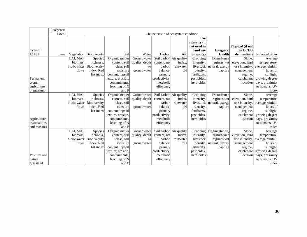
36
Type of
LCEU
Ecosystem
extent Characteristic of ecosystem condition
area Vegetation Biodiversity Soil Water Carbon Air
Use
intensity (if
not used in
land use
intensity)
Integrity.
Health
Physical (if not
in LCEU
delineation) Physical other
Permanent
crops,
agriculture
plantations
LAI, MAI,
biomass,
biotic water
flows
Species
richness,
Biodiversity
index, Red
list index
Organic matter
content, soil
class, soil
moisture
content, topsoil
texture, erosion,
contaminants,
leaching of N
and P
Groundwater
quality, depth
to
groundwater
Soil carbon
content, net
carbon
balance,
primary
productivity,
metabolic
efficiency
Air quality
index,
rainwater
pH
Cropping
intensity,
livestock
density,
fertilizers,
pesticides,
herbicides
Disturbance
regimes wrt
natural, exergy
capture
Slope,
elevation, land
use intensity,
management
regime,
catchment
location
Average
temperature,
average rainfall,
hours of
sunlight,
growing degree
days, proximity
to humans, UV
index
Agriculture
associations
and mosaics
LAI, MAI,
biomass,
biotic water
flows
Species
richness,
Biodiversity
index, Red
list index
Organic matter
content, soil
class, soil
moisture
content, topsoil
texture, erosion,
contaminants,
leaching of N
and P
Groundwater
quality, depth
to
groundwater
Soil carbon
content, net
carbon
balance,
primary
productivity,
metabolic
efficiency
Air quality
index,
rainwater
pH
Cropping
intensity,
livestock
density,
fertilizers,
pesticides,
herbicides
Disturbance
regimes wrt
natural, exergy
capture
Slope,
elevation, land
use intensity,
management
regime,
catchment
location
Average
temperature,
average rainfall,
hours of
sunlight,
growing degree
days, proximity
to humans, UV
index
Pastures and
natural
grassland
LAI, MAI,
biomass,
biotic water
flows
Species
richness,
Biodiversity
index, Red
list index
Organic matter
content, soil
class, soil
moisture
content, topsoil
texture, erosion,
contaminants,
leaching of N
and P
Groundwater
quality, depth
to
groundwater
Soil carbon
content, net
carbon
balance,
primary
productivity,
metabolic
efficiency
Air quality
index,
rainwater
pH
Cropping
intensity,
livestock
density,
fertilizers,
pesticides,
herbicides
Fragmentation,
disturbance
regimes wrt
natural, exergy
capture
Slope,
elevation, land
use intensity,
management
regime,
catchment
location
Average
temperature,
average rainfall,
hours of
sunlight,
growing degree
days, proximity
to humans, UV
index

37
Type of
LCEU
Ecosystem
extent Characteristic of ecosystem condition
area Vegetation Biodiversity Soil Water Carbon Air
Use
intensity (if
not used in
land use
intensity)
Integrity.
Health
Physical (if not
in LCEU
delineation) Physical other
Forest tree
cover
LAI, MAI,
biomass,
biotic water
flows,
deadwood
(laying and
standing),
Algae on
birch, Old
trees, soil
vegetation,
epiphytic
vegetation
Species
richness,
Biodiversity
index, Red
list index
Organic matter
content, soil
class, soil
moisture
content, topsoil
texture, erosion,
contaminants,
leaching of N
and P
Groundwater
quality, depth
to
groundwater
Soil carbon
content, net
carbon
balance,
primary
productivity,
metabolic
efficiency
Air quality
index,
rainwater
pH
Cropping
intensity,
livestock
density,
fertilizers,
pesticides,
herbicides
Fragmentation,
disturbance
regimes wrt
natural, exergy
capture
Slope,
elevation, land
use intensity,
management
regime,
catchment
location
Average
temperature,
average rainfall,
hours of
sunlight,
growing degree
days, proximity
to humans, UV
index
Shrubland,
bushland,
heathland
LAI, MAI,
biomass,
biotic water
flows
Species
richness,
Biodiversity
index, Red
list index
Organic matter
content, soil
class, soil
moisture
content, topsoil
texture, erosion,
contaminants,
leaching of N
and P
Groundwater
quality, depth
to
groundwater
Soil carbon
content, net
carbon
balance,
primary
productivity,
metabolic
efficiency
Air quality
index,
rainwater
pH
livestock
density
Fragmentation,
Disturbance
regimes wrt
natural, exergy
capture
Slope,
elevation, land
use intensity,
management
regime,
catchment
location
Average
temperature,
average rainfall,
hours of
sunlight,
growing degree
days, proximity
to humans, UV
index
Sparsely
vegetated
areas
LAI, MAI,
biomass,
biotic water
flows
Species
richness,
Biodiversity
index, Red
list index
Organic matter
content, soil
class, soil
moisture
content, topsoil
texture, erosion,
contaminants,
leaching of N
and P
Groundwater
quality, depth
to
groundwater
Soil carbon
content, net
carbon
balance,
primary
productivity
Air quality
index,
rainwater
pH
livestock
density
Fragmentation,
Disturbance
regimes wrt
natural, exergy
capture
Slope,
elevation, land
use intensity,
management
regime,
catchment
location
Average
temperature,
average rainfall,
hours of
sunlight,
growing degree
days, proximity
to humans, UV
index

38
Type of
LCEU
Ecosystem
extent Characteristic of ecosystem condition
area Vegetation Biodiversity Soil Water Carbon Air
Use
intensity (if
not used in
land use
intensity)
Integrity.
Health
Physical (if not
in LCEU
delineation) Physical other
Natural
vegetation
associations
and mosaics
LAI, MAI,
biomass,
biotic water
flows
Species
richness,
Biodiversity
index, Red
list index
Organic matter
content, soil
class, soil
moisture
content, topsoil
texture, erosion,
contaminants,
leaching of N
and P
Groundwater
quality, depth
to
groundwater
Soil carbon
content, net
carbon
balance,
primary
productivity,
metabolic
efficiency
Air quality
index,
rainwater
pH
livestock
density
Fragmentation,
Disturbance
regimes wrt
natural, exergy
capture
Slope,
elevation, land
use intensity,
management
regime,
catchment
location
Average
temperature,
average rainfall,
hours of
sunlight,
growing degree
days, proximity
to humans, UV
index
Barren land Species
richness,
Biodiversity
index, Red
list index
Organic matter
content, soil
class, soil
moisture
content, topsoil
texture, erosion,
contaminants,
leaching of N
and P
Groundwater
quality, depth
to
groundwater
Soil carbon
content, net
carbon
balance,
primary
productivity,
metabolic
efficiency
Air quality
index,
rainwater
pH
Slope,
elevation, land
use intensity,
management
regime,
catchment
location
Average
temperature,
average rainfall,
hours of
sunlight,
growing degree
days, proximity
to humans, UV
index
Permanent
snow and
glaciers
Species
richness,
Biodiversity
index, Red
list index
Parent material,
contaminants
Mass balance,
contaminants
Net carbon
balance
Air quality
index,
rainwater
pH
Open
wetlands
Number of
vegetation
classes,
invasive
species
Species
richness,
Biodiversity
index, Red
list index
Toxics in
riverbed
Streamflow
rate, hydraulic
retention time,
average size,
water quality
index
Net carbon
balance
Air quality
index,
rainwater
pH
Cropping
intensity,
hunting
intensity,
upstream
contaminant
s
Exergy capture Management
regime,
catchment
location
Average
temperature,
average rainfall,
hours of
sunlight,
growing degree
days, proximity
to humans, UV
index

39
Type of
LCEU
Ecosystem
extent Characteristic of ecosystem condition
area Vegetation Biodiversity Soil Water Carbon Air
Use
intensity (if
not used in
land use
intensity)
Integrity.
Health
Physical (if not
in LCEU
delineation) Physical other
Inland water
bodies
Number of
vegetation
classes,
invasive
species,
algae
growth on
substrate,
Species
richness,
Biodiversity
index, Red
list index,
ASPT
(average
score per
taxon),
acidifaction
index of
bottom
fauna
Toxics in
riverbed
Streamflow
rate (including
variability),
water quality
index,
chlorophyll-a
in lakes,
Net carbon
balance
Air quality
index,
rainwater
pH
Fragmentation,
exergy capture
Management
regime,
catchment
location
Average
temperature,
average rainfall,
hours of
sunlight,
proximity to
humans, UV
index
Coastal
water bodies
Number of
vegetation
classes,
invasive
species,
presence of
mangroves,
seagrass
Species
richness,
Biodiversity
index, Red
list index,
presence of
coral reefs, ,
index of
benthic
fauna
species,
Macroalgae
intertidal
index,
Macroalgae
lower limit
of growth
Coastal erosion
rate
Wave
intensity,
water quality
index
Net carbon
balance
Air quality
index,
rainwater
pH
Exergy capture Management
regime

40
Type of
LCEU
Ecosystem
extent Characteristic of ecosystem condition
area Vegetation Biodiversity Soil Water Carbon Air
Use
intensity (if
not used in
land use
intensity)
Integrity.
Health
Physical (if not
in LCEU
delineation) Physical other
Sea Number of
vegetation
classes,
invasive
species
Species
richness,
Biodiversity
index, Red
list index,
index of
benthic
fauna
species
Water quality
index,
temperature,
acidification
Net carbon
balance
Air quality
index,
rainwater
pH
Exergy capture Management
regime
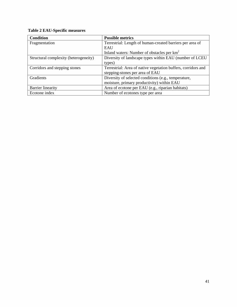
41
Table 2 EAU-Specific measures
Condition Possible metrics
Fragmentation Terrestrial: Length of human-created barriers per area of
EAU
Inland waters: Number of obstacles per km2
Structural complexity (heterogeneity) Diversity of landscape types within EAU (number of LCEU
types)
Corridors and stepping stones Terrestrial: Area of native vegetation buffers, corridors and
stepping-stones per area of EAU
Gradients Diversity of selected conditions (e.g., temperature,
moisture, primary productivity) within EAU
Barrier linearity Area of ecotone per EAU (e.g., riparian habitats)
Ecotone index Number of ecotones type per area

42
Table 3 Suggested additions to other SEEA-EEA Accounts
LCEU type Biodiversity account Asset account Carbon Account
Urban and associated
developed areas
Medium to large fields
rainfed herbaceous
cropland
Ex-situ crop collections Soil carbon content, carbon loss from
respiration, metabolic efficiency
(respiration/biomass)
Medium to large fields
irrigated herbaceous
cropland
Ex-situ crop collections Soil carbon content, carbon loss from
respiration, metabolic efficiency
(respiration/biomass)
Permanent crops,
agriculture plantations
Ex-situ crop collections Soil carbon content, carbon loss from
respiration, metabolic efficiency
(respiration/biomass)
Agriculture associations
and mosaics
Ex-situ crop collections Soil carbon content, carbon loss from
respiration, metabolic efficiency
(respiration/biomass)
Pastures and natural
grassland
Ex-situ crop collections, genetic
diversity of terrestrial
domesticated animals
Soil carbon content, carbon loss from
respiration, metabolic efficiency
(respiration/biomass)
Forest tree cover Extent of forest and forest
types, area of forest under
sustainable management
Extent of forest and
forest types, area of
forest under
sustainable
management
Soil carbon content, carbon loss from
respiration, metabolic efficiency
(respiration/biomass)
Shrubland, bushland,
heathland
Soil carbon content, carbon loss from
respiration, metabolic efficiency
(respiration/biomass)
Sparsely vegetated areas Soil carbon content, carbon loss from
respiration, metabolic efficiency
(respiration/biomass)
Natural vegetation
associations and mosaics
Soil carbon content, carbon loss from
respiration, metabolic efficiency
(respiration/biomass)
Barren land Soil carbon content, carbon loss from
respiration, metabolic efficiency
(respiration/biomass)
Permanent snow and
glaciers
Open wetlands
Inland water bodies
Coastal water bodies Extent of marine
habitats
Sea Extent of marine
habitats
All Wildlife picture index; VITEK
(Vitality of traditional
environmental knowledge);
toxins in animal tissues;
incidence of disease;
reproduction rates; age-class
distributions; indicator species;
keystone species; key species
interactions; functional and
response diversity; aggressive,
over-abundant and invasive
species; species of particular
concern (threatened, rare,
locally important); proportion
of r-selected to K-selected
species; Exotic/endemic species
Entropy production

43
Table 4 Ecological measures related to individuals, species, population and community
Level of
organization Possible metric
Individuals Toxins in tissue; incidence of disease
Species (recorded
once in a register)
Endemic/Exotic; Reproduction rates; Functional characteristics (trophic group,
size, reproductive strategy, generalist/specialist, tolerance), behavioural
characteristics (competitive, aggressive)
Population Age-class distributions, population counts, genetic variability
Community Indicator species; Keystone species; Key species interactions; species diversity