Inverse Channel Estimation Based On Adaptive Inverse Control
Ge Liu1, Zhengxin Ma
1, Yuhan Wang
1 and
1Xiaowen Shu
2
1 Department of Electronic Engineering, Tsinghua University, Beijing 100084, China
2 Military representative bureau of army aviation ,PLA, Beijing 100086, China
Abstract. A new algorithm of inverse channel estimation based on adaptive inverse control is proposed in
this paper for the multipath fading wireless channel to compensate the channel distortion. The algorithm does
not directly estimate the inverse channel, as compared with adaptive equalization. The algorithm estimates
the channel firstly, and then use offline mode for inverse channel estimation. Simulation results show that,
the new algorithm can obtain better performance in the same SNR, as compared with adaptive equalization.
Keywords: Inverse channel estimation, channel estimation, adaptive inverse control
1. Introduction
In wireless communications, wireless signal is affected by the environment, distance, propagation path
and other uncertainties, resulting in multipath and fading phenomenon and system performance degradation.
Accurate estimation of the inverse of a channel or inverse channel can transform an AWGN multipath fading
channel into an AWGN channel, thus solve the wireless channel multipath and fading problem. The most
commonly used method of inverse channel estimation is adaptive equalizer [1]. Adaptive equalizer is usually
used to directly estimate the inverse channel. The value of direct inverse channel estimation deviates from
the true value due to the presence of noise. When the signal noise ratio (SNR) is high, the inverse channel
offset is smaller, and the impact on the system performance is smaller due to lower noise. When SNR is low,
the inverse channel offset is greater, and impact on the system performance is greater.
Adaptive inverse control theory is put forward by B. Widrow in the 1980s. The basic idea is that, first
directly set up a model for an unknown object, then use the inverse object model to control the dynamic
characteristic of the object (1).
In this paper, starting from the model of wireless channel, in view of the AWGN multipath fading
channel, we propose an inverse channel estimation algorithm based on adaptive inverse control. Then,
Matlab is used in the simulation and analysis of this algorithm. Simulation results show that, by using this
algorithm in AWGN multipath fading channel to estimate the inverse channel, the estimation offset due to
noise is reduced.
2. Channel Model
Reference [3] points out, tapped delay line can be use in multipath fading channel modeling. Let’s
assume that the wireless channel is quasi static, multipath is fixed, each path loss and fading complies with
probability distribution, then, the channel impulse response shall be:
0
( ) ( ) k
Lj
k kk
h t a t t e
(1)
Where, L is the number of multipath, , ,k k ka t is respectively multipath fading coefficient, time delay
and phase. Wireless channel model can be set up by using transverse filter [4], and therefore the inverse
Corresponding author. Tel.: + 86-010-62772751; fax: +86-010-62796691.
E-mail address: [email protected].
2014 3rd International Conference on Informatics, Environment, Energy and Applications
IPCBEE vol.66 (2014) © (2014) IACSIT Press, Singapore DOI: 10.7763/IPCBEE. 2014. V66. 28
136

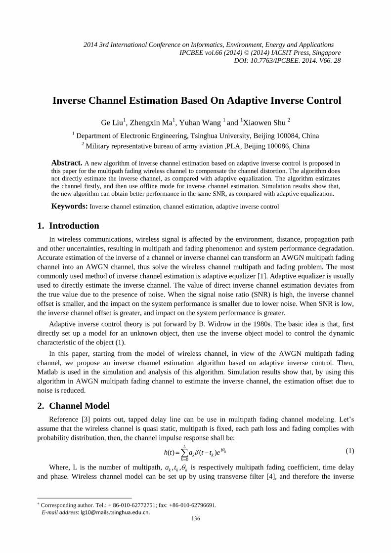
channel model can be set up with transverse filter. The adaptive equalizer, as shown in Fig. 1, is the existing
commonly used method for inverse channel estimation.
+
-
+
+
kx k
nk
z
ke
ky
H z 1ˆ ( )H z
Adaptive Algorithm
channelAdaptive Equalizer
Fig. 1. Basic Block Diagram of Adaptive Equalizer
Where,kx is the sending signal, H z is the channel transfer function,
ky is the signal after the sending
signal pass through the channel, kz is the receiving signal, 1ˆ ( )H z is the inverse channel transfer function,
kn is the additive white Gaussian noise, ke is the error.
Reference (2) put forward the Wiener solution for 1ˆ ( )H z , as shown in equation (2):
1( )( )
ˆ
( ) ( ) ( )
( )
[ ( ) ( )] ( )
( )yxzx
zz yy nn
yy
yy nn
zzH
z z z
z
z z H z
z
(2)
Where, ( )zx z is the Z transformation of kz and kx cross-correlation function, ( )zz z is the Z
transformation of kz autocorrelation function, ( )yx z is the Z transformation of kx and ky cross-correlation
function, ( )yy z is the Z transformation of ky autocorrelation function, ( )nn z is the Z transformation of
kn
autocorrelation function. kn , kx , kz are not related, so ( ) ( )zx yxz z .
As seen in equation (2), due to the existence of ( )nn z , 1ˆ ( )H z is not the inverse of H z , thus produce a
deviation. With the increase of noise power, the adaptive equalizer performance becomes worse and worse.
In order to reduce the deviation due to noise, this paper proposes a new inverse channel estimation
algorithm based on adaptive inverse control theory. The core idea is, firstly carry out channel estimation,
then estimate the inverse of the channel in offline mode, finally, the inverse channel estimation is used as a
controller to compensate for the channel.
3. Inverse Channel Estimation Algorithm Based On Adaptive Inverse Control
Because direct inverse channel estimation may be affected by noise, three steps are taken to estimate the
channel inverse:
3.1. Channel Estimation
The basic block diagram for channel estimation is shown in Fig. 2.
+
-
+
+
kx
kn
kz
ke
ky( )H z
ˆ ( )H zˆk
x
Adaptive Algorithm
Fig. 2. Basic Block Diagram of Channel Estimation
Where, ˆ ( )H z is the estimation of channel transfer function.
Reference (2) put forward the Wiener solution for ˆ ( )H z , as shown in equation (3):
( )( ) ( ) ( )
ˆ ( )( ) ( ) ( )
( )xyxz xx
xx xx xx
zz z H zH H z
z z zz
(1)
137
Where, ( )zx z is the Z transformation of kx and kz cross-correlation function, ( )xy z is the Z
transformation of kx and ky cross-correlation function, ( )xx z is the Z transformation of ky autocorrelation
function, Because kn , kx , kz are not related, ( ) ( )xz xyz z .
As seen in equation (3), when there is a kn , as long as kn and kx are not correlated, then ˆ ( )H z can
accurately estimate H z .
In order to follow the time-varying characteristics of the channel, adaptive filter is used in h(n)
modeling estimation. Due to the existence of noise, the error ke cannot be zero, so the method of recursive
least square (RLS) of the variable forgetting factor (VFF) [5] is used in channel estimation. The purpose of
variable genetic factor is to enable ˆk k
x x and k ke n . When is small, ke tends to zero. When 1 ,
significant error will be introduced. In order to avoid a large imbalance, must be limited inside the closed
interval of around 1. The adaptive filter will take a known sending training sequence ( ) kx n x as the input,
the desired signal ( ) kd n z , the recursive equation of VFF-RLS algorithm is as follows:
1*
1
1
2 2
( ) ( 1) ( )ˆ ˆ( ) , ( ) ( ) ( 1) ( ), ( ) ( 1) ( ) ( ),
1 ( ) ( ) ( 1) ( )
ˆ ˆ( ) ( ) (1 ( ) ( )) ( 1), ( ) ( ) ( ), ( ) ( ) ( ) ( ),
( ) ( ) ( 1) ( ), ( 1) ( ) (1
H
H
H H H
H
n P n x nk n n d n w n x n w n w n k n n
n x n P n x n
P n n k n x n P n y n w n x n e n d n w n x n
q n x n P n x n n n
2 2 2 2
2 2 2
min max1
2 2 2
) ( ), ( 1) ( ) (1 ) ( ),
( ) ( )( 1) ( ) (1 ) ( ), ( ) , ( ) min[max( , ( ), ].
[ ( ) ( )]
q q
q e
e e
e
n n n q n
n nn n e n n n n
n n
(2)
1 11 , 1 , 1K K
K N K N
,N is the length of the filter. When the VFF-RLS converges to a fixed
value, ˆ ˆ ( )h n w n .
3.2. Channel Estimation
The inverse channel stability depends on whether the channel transfer function is at minimum phase or
not. A stable inverse channel can be obtained in the following two cases:
3.2.1 Minimum Phase
When the channel transfer function is at minimum phase, the transfer function zeros are within the unit
circle, that is to say, its inverse poles are also inside the unit circle, the inverse channel is stable. The basic
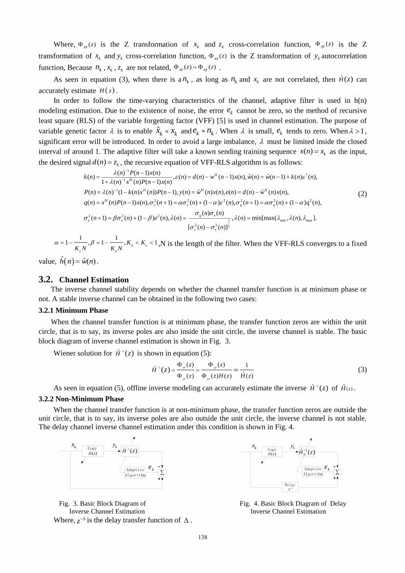
block diagram of inverse channel estimation is shown in Fig. 3.
Wiener solution for 1ˆ ( )H z
is shown in equation (5):
1( ) ( ) 1
ˆˆ( ) ( ) ( ) ( )
( )yx yy
yy yy
z zH
z z H z H zz
(3)
As seen in equation (5), offline inverse modeling can accurately estimate the inverse 1ˆ ( )H z
of ( )ˆ zH .
3.2.2 Non-Minimum Phase
When the channel transfer function is at non-minimum phase, the transfer function zeros are outside the
unit circle, that is to say, its inverse poles are also outside the unit circle, the inverse channel is not stable.
The delay channel inverse channel estimation under this condition is shown in Fig. 4.
+
-
kx
ˆ ( )H z1ˆ ( )H z
ke
ky
Copy
Adaptive Algorithm
+
-
kx
ˆ ( )H z1ˆ ( )H z
ke
ky
z
Adaptive Algorithm
Delay
Copy
Fig. 3. Basic Block Diagram of Fig. 4. Basic Block Diagram of Delay
Inverse Channel Estimation Inverse Channel Estimation
Where, z is the delay transfer function of .
138

The purpose of using z to eliminate the zero points of channel transfer function outside the unit circle,
that is multiply ( )ˆ zH and 1ˆ ( )H z
, the result is the best fitting for z . The selecting of value is very
important. If the value selected is too small, the transfer function cannot be stable. If the value is too big, a
more ideal time delay inverse can be obtained, but the time delay of the output signal will be bigger.
Therefore, the commonly used Δ empirical value is half the length of the filter. As for the minimum phase
system, delay Δ = 0 is a good option.
A modified MNLMS algorithm proposed in reference (6) can be used in inverse channel estimation..
Adaptive filter can take ( ) kx n y as the input, where the parameter ˆ( )h n can copy the estimation value of
the above step, the desired signal is ( ) kd n x , the recursive equation for MNLMS algorithm is as follows:
2
2
1
ˆ ˆ( ) ( ) ( ), ( ) ( ) ( ) ( )
ˆ ˆ1
1
H H
n
i
i
y n w n x n e n d n w n x n
w n w n e n n
n
e
x
x
(6)
Where, is the step length, 0,0 1 . When MNLMS is converged to a fixed value, 1ˆ ˆ ( )h n w n
.
3.2.3 Adaptive Inverse Control of the Channel
The basic block diagram of the channel adaptive inverse control is shown in Fig. 5.
+
+
kx
kn
kzky( )H z
1ˆ ( )H z
Copy
Fig. 5. Basic Block Diagram of the Channel Adaptive Inverse Control
After the inverse channel estimation 1h n
is obtained, the estimation can be used as a controller
connected in series to the receiver front-end, so as to compensate the influence of channel on the signal.
4. Simulation Results
Simulation parameter settings are as follows: QPSK modulation is adopted, signal symbol rate is 2.5
Mbps, sampling rate is 16, roll-off factor of forming and matched filtering is 0.35, channel impulse response
is 0.6708 0.5 0.3873 0.3162 0.2236h n , channel noise is additive white Gaussian noise. VFF-RLS algorithm
is used in channel estimation, 0.5K , 0.05K
, min 0.9965 , max 0.999999 . Both the inverse channel
estimation and adaptive channel equalization adopts the MNLMS algorithm, 0.2 , 0.8, 0.4 .
Fig. 6 shows the signal amplitude difference in the case of SNR = 0 db. In this case, the adaptive inverse
control and adaptive equalization are used respectively in inverse channel estimation. Receiving signal with
no noise respectively pass through the inverse channel estimator, producing a signal that is different from the
sending signal. The figure shows that the receiving signal passed through the adaptive inverse control
estimation or the channel inverse filter is better than the signal of the adaptive equalizer, namely closer to the
send signal, therefore it can better compensate the influence of channel on the signal.
Fig. 6. Signal Amplitude Difference in Case of SNR=0db
Fig. 7 and Fig. 8 respectively show the frequency response in the case of SNR = 0 db and SNR = 20 db.
The adaptive inverse control and adaptive equalization are used respectively in inverse channel estimation.
After the inverse channel estimation is obtained, we can see the combined frequency response of the channel
and the inverse channel. Ideally, the system with the channel and the inverse channel connected in series is
an all-pass system. As shown in the two figures, with the same SNR, using adaptive inverse control in
inverse channel estimation, the system will be a near all-pass system. The system bandwidth is wider than
that of the system which uses the adaptive equalization algorithm for inverse channel estimation. It also has a
139

better in-band flatness and better basic linear phase. As SNR gradually degrading, the performance of inverse
channel estimation by using adaptive equalization algorithm deteriorates. But the performance of inverse
channel estimation by using adaptive inverse control algorithm will not be seriously impacted.
Fig. 7. Frequency Response in the Case of SNR=0db
Fig. 8. Frequency Response in the Case of SNR=20db
Fig. 9 shows the system bit error rates (BER) in the cases of different SNRs. As shown in the figure,
with the same SNR, the BER in the case of using the inverse channel estimation algorithm based on adaptive
inverse control is lower than that of using the adaptive equalization algorithm.
Fig. 9. Bit Error Rates
5. Conclusions
This paper studies the problem of inverse channel estimation for the multipath fading channel in
wireless communication. The inverse channel estimation algorithm based on adaptive inverse control is
proposed. Using the algorithm can transform an AWGN multipath fading channel into an AWGN channel.
Theoretical analysis results show that this algorithm can suppress noise influence on inverse channel
estimation. Modeling and simulation and analysis are conducted on this algorithm. As compared with the
traditional adaptive equalization algorithm, this algorithm is less affected by noise, can more accurately
estimate the channel inverse. With the same SNR, the new algorithm has lower bit error rates.
6. References
[1] Chen T, Zakharov Y V, Liu C. “Low-Complexity Channel-Estimate Based Adaptive Linear Equalizer, ” Signal
Processing Letters, IEEE, 2011, 18(7): 427-430.
[2] B. Widrow, “Adaptive Inverse Control”, Adaptive System in Control and Signal Processing, Sweden, 1986.
[3] Zhan Yi. “Variable step size LMS adaptive equalization algorithm and its implementation on
DSP, ”Chengdu:University of Electronic Science and Technology of China.2010.11
[4] Heping, Xu bingxiang,Zhanghui,Feng maoguan, “Adaptive Equalization Technique Application to Time-Variant
Fading Channels, ” Aota Electronica Sinica,1993,4:85-89.
[5] TIANWen-ke,WANGJian,SHANXiu-ming, “Adaptive Equalization Technique Application to Time-Variant
Fading Channels, ” Telecommunication Engineering,2011,9:78-82.
[6] HAN Hua, LUO An, “Modified NLMS Algorithm and Its Smiulation Research in Adaptive Inverse Control, ”
Measurement & Control Technology,2008,5,:74-77.
140