


Influence of viscous layers on the growth of normal faults: insights from
experimental and numerical models
Nicolas Bellahsena,b,*, Jean-Marc Daniela, Laurent Bollingerc, Evgenii Burovb
aDivision Geologie–Geochimie, Institut Francais du Petrole, 1 et 4 avenue de Bois Preau, Rueil Malmaison 92852, FrancebUniversite Pierre et Marie Curie, Paris 6, France
cLDG, CEA, Bruyeres le Chatel, France
Received 30 November 2001; accepted 21 October 2002
Abstract
The influence in space and time of viscous layers on the deformation pattern of brittle layers is investigated using wet clay/silicone putty
analogue models in extension. Brittle and brittle–viscous experiments at various extension velocities are compared. Numerical models are
also performed to confirm the results and to control the boundary conditions. Our results show that: (i) the presence of a basal viscous layer
localizes the deformation by creating faults with very large throw. This kind of deformation distribution constrains the location of small
faults, with scattered orientations, in the vicinity of the larger, in particular in relay zones. (ii) A lower strength of the viscous layer (i.e. a low
extension velocity) enhances this localization of the deformation. (iii) The displacement–length relationship and the spatial distribution of
small-scale faults are strongly influenced by both the rheology of the model and the amount of extension. This study shows that they are
important parameters, especially when characterizing the whole fault network evolution and the relationship between large and small faults.
q 2003 Elsevier Science Ltd. All rights reserved.
Keywords: Normal faults; Analogue models; Numerical models; Viscous layers; Rheology; Displacement–length relationship
1. Introduction
Geometry, spacing and growth sequence are fault-
network characteristics commonly explained in terms of
both the rheology and the thickness of the brittle layer in
which faults grow (Vendeville et al., 1987; Cowie and
Scholz, 1992b; Cowie et al., 1993; Lavier et al., 1999;
Ackermann et al., 2001). Using field studies, experimental
and numerical models, a sequence of propagation for
normal faults has been described as the combination of
radial propagation (growth of an isolated fault by tip
propagation) and segment linkage (Fig. 1) (Segal and
Pollard, 1980; Peacock and Sanderson 1991; Cowie and
Scholz, 1992b; Cowie et al., 1993; Cartwright et al., 1996;
Marchal et al., 1998; Ackermann et al., 2001).
When the evolution of a complete fault network is
described through statistical studies, two relationships are
often computed: the displacement–length relationship and the
size–frequency relationship. Both are characterized by
power-law type functions (Watterson, 1986; Walsh and
Watterson, 1988; Cowie and Scholz, 1992a; Dawers et al.,
1993; Scholz et al., 1993; Clark and Cox, 1996; Nicol et al.,
1996; Pickering et al., 1997; Cowie, 1998) and can be applied
to estimate the strain contribution and the characteristics of
small-scale faults. The following power-law relation
expresses the displacement (D)–length (L) relationship:
D ¼ cLn ð1Þ
where c is the function of the mechanical characteristics of the
layer, and n is the scaling exponent. Values for this exponent
range from less than 1 (Fossen and Hesthammer, 1997; Gross
et al., 1997; Ackermann and Schlische, 1999), to 1 (Cowie and
Scholz, 1992a; Dawers et al., 1993; Schlische et al., 1996), 1.5
(Marrett and Allmendinger, 1991; Gillespie et al., 1992;
Yielding et al., 1996) and, 2 (Watterson, 1986; Walsh and
Watterson, 1988). Although most investigators agree that a
value of 1 is a good rule, no consensus has yet been established
about the value of n.
The presence of viscous layers and their strength are
known to be important parameters controlling deformation
0191-8141/03/$ - see front matter q 2003 Elsevier Science Ltd. All rights reserved.
PII: S0 19 1 -8 14 1 (0 2) 00 1 85 -2
Journal of Structural Geology 25 (2003) 1471–1485
www.elsevier.com/locate/jsg
* Corresponding author. Current address: Dept. of Geological and
Environmental Sciences, Stanford University, Stanford CA94305-2115,
USA.
E-mail address: [email protected], nicolas.bellahsen@lgs.
jussieu.fr (N. Bellahsen).

patterns. The importance of the mechanical layering has
been demonstrated for the lithosphere (Allemand and Brun,
1991; Buck et al., 1999; Brun, 1999), the whole crust (Brun,
1999), and the upper brittle crust (Gross et al., 1997;
Withjack and Callaway, 2000). The effects of brittle
mechanical layering on fault network growth have been
studied recently in an experimental work (Ackermann et al.,
2001) and from field data (Schultz and Fossen, 2002).
However, the effects of viscous layers have been under-
studied, except in Davy et al. (1995) in a compressive
context or in Withjack and Callaway, (2000) in basement-
involved faulting.
In this paper, analogue and numerical models are used to
demonstrate the influence of viscous layers on fault growth.
For this purpose, fault networks generated with and without
a basal viscous layer, and networks generated with a basal
viscous layer under various extension velocities are
compared. In each experiment, the general space-time
evolution of normal fault networks is studied through three
steps of extension, with particular attention paid to the
spatial relationships between large and small faults.
2. Experimental procedure and dataset
2.1. Experimental set-up and materials
2.1.1. Boundary conditions
The experiments are performed in a deformation box
(Fig. 2), with dimensions ranging between 60 £ 50 £ 10 and
60 £ 70 £ 10 cm. A basal rubber sheet fixed to rigid and
movable walls induces nearly homogeneous extension in
the overlying materials. The rubber sheet can be affected by
strain gradients in the vicinity of the movable wall,
especially at high extension rates and with a thick rubber
sheet (Ackermann, 1997). This small departure from
homogeneous extension affects the fault related strain but
does not alter the results presented later in this paper. Fault
networks are generated in a two-layer model, one 2 cm
silicone lower layer and one 4 cm wet clay upper layer. Five
experiments in a suite of 15 are used to demonstrate the
influence of viscous layer on fault growth.
2.1.2. Analogue materials and scaling laws
The wet clay used here consists of a homogeneous
mixture of water and pure industrial kaolinite powder. This
kind of material has been previously used to simulate brittle
behaviour (Cloos, 1968; Withjack and Jamison, 1986;
Clifton et al., 2000; Withjack and Callaway, 2000;
Ackermann et al., 2001). The water/kaolinite mixture in
our experiments has a density of 1.55 g/cm3 (approximately
40% water). At the conditions and scale of the experiments,
the wet clay behaves like a brittle material in which faults
develop as illustrated in Fig. 3. The internal friction of the
wet clay is about 0.5 (Sims, 1993). This value is similar to
Fig. 1. Normal fault growth (from Cowie, 1998). (a) Isolated growth by tip
propagation. (b) Interactions between fault segments. (c) Propagation by
segment connection.
Fig. 2. Experimental set-up: the deformation box in cross-section. Two
layers compose the model: one 4 cm thick layer of sand, one 2 cm thick
layer of silicone. The two-layer model is underlain by a basal rubber sheet
that applied the extension, whose velocity varied from 0.011 to 0.05 mm/s.
Fig. 3. Surface view of the fault network generated in wet clay. (a)
Curvature of a fault segment and beginning of the coalescence. (b)
Curvature of two segments leading to a single and undulating fault.
N. Bellahsen et al. / Journal of Structural Geology 25 (2003) 1471–14851472

the internal friction of rocks in nature. The cohesion of the
wet clay is estimated to 50 Pa (Sims, 1993). As inertial
forces are neglected, the cohesion must satisfy the following
dynamic similarity criterion:
Cp ¼ dpgplp ð2Þ
where C p, d p, g p, and l p are the model-to-nature ratio
for cohesion, density, gravity, and length, respectively
(Hubbert, 1937). In our models, C p is about 1024–1025, d p
is about 0.6, and g p is equal to 1. Thus, to ensure dynamic
similarity and satisfy Eq. (2), the length ratio l p is about
1.5 £ 1024–1.5 £ 1025 (1 cm in the model corresponds to
about 60–600 m in nature).
The silicone putty (SMG36 produced by Dow Corning)
is used to simulate viscous layers such as salt or under-
compacted shales layers in sedimentary basins. The silicone
putty, under laboratory conditions, behaves as a Newtonian
fluid (Weijermars, 1986) with a viscosity equal to 5.104 Pa s
and a density of 0.97 g/cm3. The silicone putty must satisfy
the following similarity criterion:
hp ¼ dpgplptp ð3Þ
where h p, d p, g p, l p, and t p are the model-to-nature ratio
for viscosity, density, gravity, length, and time, respect-
ively. In our models, h p is about 10214, d p is about 0.6, g p
is equal to 1, and l p is about 1.5 £ 1025. Thus, to satisfy Eq.
(3), t p is about 1029 (1 h in the model represents about
100,000 years in nature).
Two parameters were varied: the presence of basal
silicone putty and the velocity of extension. Two exper-
iments were performed without silicone at two different
velocities (0.023 and 0.05 mm/s), and three experiments
were performed with basal silicone putty at three different
velocities (0.011, 0.023 and 0.05 mm/s). The models are
deformed at strain rates between 2 £ 1025 s21 and
1024 s21. The last value is similar to Ackermann et al.
(2001). This lower velocity is used to explore the role of low
silicone strength, as it is proportional to velocity (and
viscosity):
R ¼ hhe 0 ð4Þ
where R, h, h, and e 0 are the strength, the thickness, the
viscosity and the strain rate of the silicone layer,
respectively. The extension is transmitted from the base of
the model and then is different from a far-field extension.
Questions could also arise from the coupling between the
rubber sheet and the silicone and between the silicone and
the sand layer. These experimental conditions are discussed
in a later section.
Finally, as illustrated in Section 3.1 and reported by
recent works (Clifton et al., 2000; Ackermann et al., 2001),
the modes of faulting in wet clay are close to natural brittle
deformation. Thus, although the models might not be
perfectly scaled, they are useful to simulate natural
extensional features.
2.2. Data processing
2.2.1. Fault detection
The deformed models are analyzed using topographic
information. A three-dimensional (3D) laser-beam scanner
allows us to digitize the model topography (Fig. 4a) and
build a digital elevation model in the central part of the
experiment avoiding edge effects. The laser resolution is
0.25 mm in the x, y, z directions. From this topographic data,
a slope map is calculated using a gradient matrix. Fault
surfaces are extracted by fixing a threshold on the slope map
(Fig. 4b). This map contains three values: (i) white for low
slope area, (ii) blue for west, and (iii) red for east dipping
faults. The last step consists of the automatic digitization of
the fault polygons (Fig. 4c). As the fault polygons are
extracted from the topographic map, each segment building
these polygons is contained in a 0.25 £ 0.25 mm cell.
Finally, the fault polygons that crosscut the edge of the
analyzed area are automatically removed from the fault list.
The topographic map and the list of fault polygons contain
the entire information about the 3D-fault surface (i.e. x, y, z
coordinates, strike, dip direction, length, throw). These
parameters are used to quickly compute scaling relation-
ships such as the displacement–length relationship.
2.2.2. Displacement–length relationship
Below a throw of about 0.25 mm, fault length is
underestimated and the trend of the dataset in this area
has a lower slope than in the large length area (Fig. 5). For
this reason, the throw length relationship is calculated in the
area of medium to large throw and length (i.e. the data in the
black continuous envelope in Fig. 5). The relationship is
then calculated over one order of magnitude of length and
throw.
For practical reasons, the throw–length relationship will
be used in this paper as a proxy for the displacement–length
relationship with the implicit assumption that all the faults
have the same dip. Nonetheless, faults tend to rotate with
increasing applied strain and their dip decreases from an
initial value of 708 to about 558. Long faults have generally a
longer history than short faults, they have accumulated more
displacement and rotation toward lower dip. Therefore, the
throw–length plot underestimates the contribution of large
faults with respect to a displacement–length plot. Quanti-
tatively, the slope of the throw–length relationship in a
log/log plot should be lower than the one that would have
been measured on a log/log displacement/length plot.
However, we keep the throw–length relationship as a
proxy for the displacement–length relationship because we
are not interested in the absolute value of the displacement–
length slope and this bias mainly affects the very late stages
of the experiments.
2.2.3. Deformation map and participation ratio
From the map of fault polygons and measured throw,
‘deformation’ maps can be computed to study the spatial
N. Bellahsen et al. / Journal of Structural Geology 25 (2003) 1471–1485 1473

organization of deformation associated with faulting. A cell
of these deformation maps can contain several fault
segments. In each cell, we calculate the product of the
length of each small segment of the faults (see Section
2.2.1) with the associated throw. The value d of each cell of
the deformation map is then the sum of all these products.
This measure is linearly related to strain, under the
assumption that faults are dip-slip and have a more-or-less
constant dip. Several deformation maps are computed
changing the cell size. An increase of the cell size
Fig. 4. Steps of the data processing. (a) Digital topography of the model. (b)
Fault surfaces obtained from a gradient map and using a threshold on slopes
(high gradients). (c) Map of the faults represented by their outline (polygons),
which contains all the geometrical information (azimuth, length, throw and dip).
Fig. 5. Calculation of displacement–length relationship and effect of
resolution. In log–log representation, the scatter of data is similar to the
scatter of natural data. We see also the scatter linked to the resolution of the
experimental system (multiples of 0.25 mm). The continuous envelope is
the data envelope. The black one (continuous and dashed) is the envelope
that we would have obtained without resolution problems: at small throws,
the length is underestimated. The displacement–length relationship is
computed only with the data in the continuous black envelope.
N. Bellahsen et al. / Journal of Structural Geology 25 (2003) 1471–14851474

corresponds to a resolution decrease. These deformation
maps are then used to estimate the distribution of the
deformation and its localization. The localization is the
capacity of the deformation to be distributed heteroge-
neously in system (Davy et al., 1995). A participation ratio
P is used to quantify the localization (Davy et al., 1995;
Sornette et al., 1993). This ratio is defined as:
P ¼1
S
ðP
dÞ2Pd2
ð5Þ
where S is the total number of pixels in the map, d the value
of each cell of the deformation map (see above). P compares
areas affected by deformation with the total area; a lower
ratio indicates greater localization (Davy et al., 1995). P is
computed for three experiments with basal silicone putty
and two experiments without basal silicone putty, from
deformation maps that have been computed with various
resolutions (Fig. 6). When the resolution decreases (large
size of cell), the participation ratio increases because a low
resolution has the effect of diffusing the measure of the
deformation. From Fig. 6, we see that two curves cross at
certain resolutions. These crossings are artefacts caused by
measurement inaccuracy. In this case, we consider the
curves identical.
2.2.4. Measured extension versus applied extension
Due to the resolution dependency of P, a second
quantitative method is used, where the ratio E between the
measured extension and the applied extension is calculated.
Heaves are summed along cross-sections in the extension
direction and a ratio is calculated with these heave sums
over the extension applied. This ratio E is plotted versus the
extension applied (Fig. 7) for the five experiments. As
expected, this ratio is smaller than one because the applied
extension is accommodated by continuous deformation of
the wet clay layer (Ackermann et al., 2001) and by small
faults not detected by the laser (throws below 0.25 mm).
Thus, this ratio is an indicator of the relative importance that
the deformation accommodated for small-scale features: a
higher ratio indicates a larger contribution of the large faults
on deformation. As explained above in the case of the
participation ratio, some curves cross. These crossings are
not significant and the crossing curves can be considered as
identical.
3. Results
3.1. Fault network characteristics and scaling relationships
In the experiments, faults propagate by a combination of
two mechanisms: (i) radial propagation (isolated growth by
tip propagation) and (ii) segment linkage (Fig. 8). The radial
propagation is the most important mechanism during the
early stages of extension (Fig. 8a). Faults grow separately,
their displacement and length are increasing simultaneously
to produce quite symmetric throw profiles. Faults then start
to interact when their length is sufficiently large to create
overlap (Fig. 8b). In this case propagation is disturbed,
throw profiles become asymmetric and throw increases
faster than length. After this period of interaction, the two
Fig. 6. Participation ratio P as a function of the resolution. This ratio is
calculated for different sizes (0.25–100 mm) of pixel of the deformation
map. A large pixel means a low resolution. The deformation is localized
(low value of P) when this ratio is small. Here the ratio is smaller in the case
of a low extension velocity. The deformation is then particularly localized
with low strength silicone.
Fig. 7. Measured extension/applied extension ratio E as a function of the
extension. This ratio is higher when the extension is accommodated by
faults above the laser resolution. When the extension velocity is high, very
small faults are numerous and E is low. When E is high, the extension is
accommodated by large faults; the deformation is more localized, as in the
low velocity case.
N. Bellahsen et al. / Journal of Structural Geology 25 (2003) 1471–1485 1475

segments frequently link (Figs. 3 and 8c). Connections can
also occur before the formation of a relay zone when the
segments turn toward each other before propagating fault
tips overlap (Fig. 3). The resulting fault shows typical
undulations and an irregular throw profile (Fig. 8c). As
already reported by Clifton et al. (2000) and Ackermann
et al. (2001), the propagation sequence of faults in the wet
clay is closely similar to the propagation sequence of natural
faults.
Quantitatively, the maximum displacement (D)–length
(L) relationship has been computed for three steps of
extension of each experiment and is characterized by the
relation expressed by Eq. (1). The scatter exhibited by the
data (Fig. 5) has been frequently observed and explained by
the mechanism of segment linkage both in natural fault
networks (Cartwright et al., 1995) and other analogue
models (Mansfield and Cartwright, 2001). The scatter at low
displacement values is also caused by the resolution of the
laser beam (0.25 mm) and the related inaccuracy of throw
and length measurements. The scaling exponent n of the
different fault networks varies between 0.6 and 1 (Table 1).
These values are consistent with those obtained by
Ackermann et al. (2001) and in some natural cases (Fossen
and Hesthammer, 1997; Gross et al., 1997; Ackermann and
Schlische 1999).
3.2. Localization of deformation
Even though the effects of mechanical properties and
thickness of a brittle layer on fault patterns are well known,
the effects of a viscous layer underlying a brittle layer are
still not well documented. Therefore, we compare the
distribution of deformation on one-layer wet clay and two-
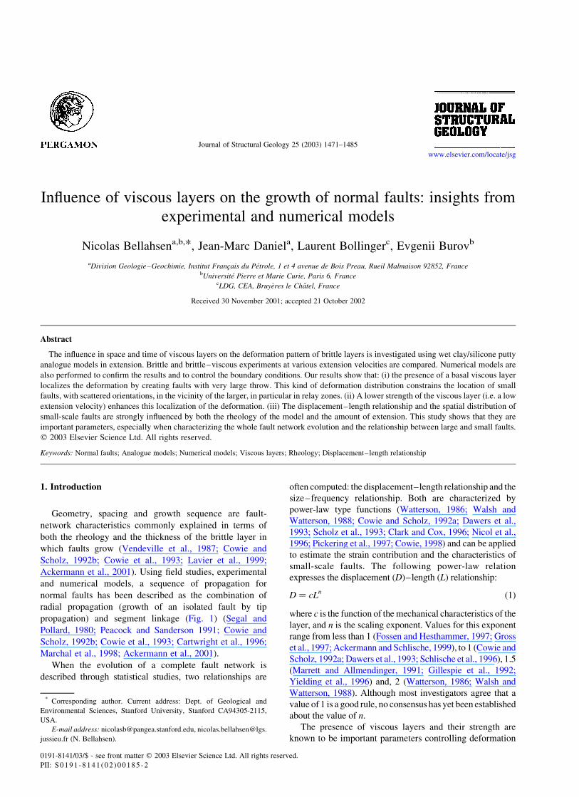
layer wet clay/silicone models (Fig. 9). The first stages of
extension (less than 7%) are difficult to analyze because the
size of the faults is commonly below the resolution of the
laser beam, and also because some extension may be
accommodated by continuous deformation. Even though the
networks are quite similar, the distribution of the defor-
mation is clearly more heterogeneous and the maximum
displacements are more important with a basal viscous
layer. When extension values are larger than 15%, the
evolution of the two fault networks is very different.
Without the silicone layer, new faults initiate and grow
continuously, resulting in a relatively homogeneous fault
pattern. In contrast, in the presence of a basal silicone layer,
few faults initiate and develop, accommodating the major
part of the applied extension. This style of deformation
produces non-deformed zones bounded by faults with large
displacement. The participation ratio P (Fig. 6) quantifies
the difference between clay and clay/silicone models. At a
fixed resolution, the ratio P calculated for clay experiments
is systematically higher than in clay/silicone experiments,
whatever the velocity (see, for example v ¼ 0.023 mm/s of
the experiment displayed in Fig. 9). The ratio E of measured
extension over applied extension (Fig. 7) allows us to study
how the model accommodates the extension. Large ratios
(close to one) indicate that large faults develop. Low ratios
indicate that the extension is accommodated by smaller
faults (and very small faults not well detected). The ratio E
Fig. 8. Growth sequence observed in the clay models. Topography map and
throw profiles are shown. (a) Two faults grow by tip propagation. The
maximum throw is about 4 mm. (b) The faults start to interact and a
segment turns toward the other one. The maximum throw is about 7 mm. (c)
Both the segments are connected and form a single fault (another is
connected on the left of the map). At this last step, the maximum throw is
10 mm.
Table 1
List of scaling exponent of displacement–length relationship for each
experiment. The three steps of extension are computed (Ext.: amount of
extension). Sil.: two-layers experiments (sand and silicone putty). Three
exponents are not given because regression was not satisfactory
Ext. 13% Ext. 20% Ext. 28%
0.05 mm/s 0.59 0.68
0.023 mm/s 0.64 0.66
Sil. 0.05 mm/s 0.80 0.76
Sil. 0.023 mm/s 0.83 0.87 0.85
Sil. 0.011 mm/s 0.77 0.89 0.97
N. Bellahsen et al. / Journal of Structural Geology 25 (2003) 1471–14851476
for experiments with basal silicone layer is systematically
higher than in experiments without basal silicone. Fault
networks in clay/silicone models are composed of faults
with a statistically larger displacement than in clay models.
This observation, combined with qualitative comparison of
network and results of participation ratio calculation,
highlights that the deformation is more localized in models
with a basal silicone layer.
In wet clay/silicone models, an important parameter is
the extension velocity as it controls the strength of the
viscous layer (Eq. (4)). Its effects on the fault network are
studied comparing the networks generated in clay and
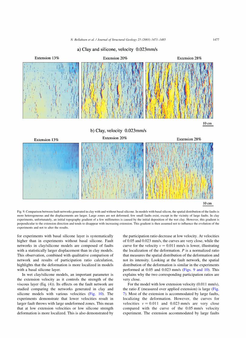
silicone models with various velocities (Fig. 10). The
experiments demonstrate that lower velocities result in
larger fault throws with large undeformed zones. This mean
that at low extension velocities or low silicone strength
deformation is more localized. This is also demonstrated by
the participation ratio decrease at low velocity. At velocities
of 0.05 and 0.023 mm/s, the curves are very close, while the
curve for the velocity v ¼ 0.011 mm/s is lower, illustrating
the localization of the deformation. P is a normalized ratio
that measures the spatial distribution of the deformation and
not its intensity. Looking at the fault network, the spatial
distribution of the deformation is similar in the experiments
performed at 0.05 and 0.023 mm/s (Figs. 9 and 10). This
explains why the two corresponding participation ratios are
very close.
For the model with low extension velocity (0.011 mm/s),
the ratio E (measured over applied extension) is large (Fig.
7). Most of the extension is accommodated by large faults,
localizing the deformation. However, the curves for
velocities v ¼ 0.011 and 0.023 mm/s are very close
compared with the curve of the 0.05 mm/s velocity
experiment. The extension accommodated by large faults
Fig. 9. Comparison between fault networks generated in clay with and without basal silicone. In models with basal silicon, the spatial distribution of the faults is
more heterogeneous and the displacements are larger. Large zones are not deformed; few small faults exist, except in the vicinity of large faults. In clay
experiments, unfortunately, an initial topography gradient of a few millimetres is caused by the initial deposition of the wet clay. However, this gradient is
perpendicular to the extension direction and tends to disappear with increasing extension. This gradient is then assumed not to influence the evolution of the
experiments and not to alter the results.
N. Bellahsen et al. / Journal of Structural Geology 25 (2003) 1471–1485 1477
is effectively almost the same for the two experiments
(0.011 and 0.023 mm/s). This result combined with that of
the participation ratio provides interesting information. For
fast extension velocity (i.e. 0.05 mm/s), the deformation is
‘homogeneously’ distributed. For lower extension velocity
(i.e. 0.023 mm/s), the deformation is also ‘homogeneously’
distributed, but the extension is accommodated by larger
faults. Finally, for the lowest extension velocity (i.e.
0.011 mm/s), the deformation is more heterogeneously
distributed and the extension accommodated by large faults
is similar to the one of the previous experiment. In
summary, these experiments show that: (i) the presence of
a basal viscous layer induces a localization of the
deformation, and (ii) a low extension velocity, applied at
the base of the model, enhanced this phenomenon.
3.3. Small faults
So far we have demonstrated that the characteristics of
the viscous layer strongly influence the geometry of the fault
pattern as a whole. This section demonstrates that its effect
is also significant when describing the relationship between
large and small faults.
Large faults generated in analogue models with strongly
localized deformation accommodate most of the applied
extension. In this case, the creation of new major faults is
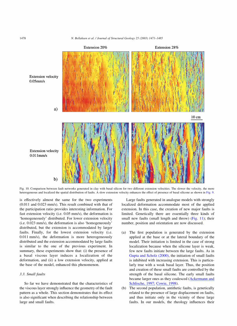
limited. Genetically there are essentially three kinds of
small new faults (small length and throw) (Fig. 11); their
number, position and orientation are now discussed.
(a) The first population is generated by the extension
applied at the base or at the lateral boundary of the
model. Their initiation is limited in the case of strong
localization because when the silicone layer is weak,
few new faults initiate between the large faults. As in
Gupta and Scholz (2000), the initiation of small faults
is inhibited with increasing extension. This is particu-
larly true with a weak basal layer. Thus, the position
and creation of these small faults are controlled by the
strength of the basal silicone. The early small faults
became larger ones as they coalesced (Ackermann and
Schlische, 1997; Cowie, 1998).
(b) The second population, antithetic faults, is genetically
related to the presence of large displacement on faults,
and thus initiate only in the vicinity of these large
faults. In our models, the rheology influences their
Fig. 10. Comparison between fault networks generated in clay with basal silicon for two different extension velocities. The slower the velocity, the more
heterogeneous and localized the spatial distribution of faults. A slow extension velocity enhances the effect of presence of basal silicone as shown in Fig. 9.
N. Bellahsen et al. / Journal of Structural Geology 25 (2003) 1471–14851478
number as a weak silicone layer, producing large
displacements, induces the creation of a large number
of these faults. Meanwhile, their position and their
orientation, which is parallel to the direction of the
large faults, remain unchanged.
(c) The third population is generated in zones of
interaction between two faults. This last kind of
small faults is the population of faults created
particularly in the case of relay ramp fracturing. The
orientation of these faults is oblique to the average
strike of the larger ones.
The measure of the dispersion of fault orientation
(Fig. 12) gives two results. The first is a greater dispersion
of small faults than larger ones. The activity of a large fault
perturbs the stress field, in particular the directions of
principal stresses around normal faults (Simon et al., 1999).
Near the centre of the fault, stress releases occur, especially
in the footwall block. At the fault tips, stress accumulations
and perturbations (Kattenhorn et al., 2000) and interactions
between faults (Crider and Pollard, 1998) perturb the stress
field in relay zones. The orientation of principal stresses is
then changed and new small faults initiate according to this
local stress field. These perturbations should be enhanced by
the accumulation of displacement on large faults. Thus, the
phenomenon is amplified with the evolution of the system,
as an increase of total extension applied induces an increase
of the throws and lengths of faults. The second result of
Fig. 12 shows the increase of this dispersion with the
decrease of silicone strength. This effect is explained by the
increase of localization at low silicone strength that
contributes to create large faults and then increases the
role of relay zones, stress field perturbations, and dispersion
of small fault directions.
From what we have seen so far, the position of small
faults was influenced by the strength of the basal silicone
layer and small faults are clustered around large faults when
the basal layer is weak, as only small relay faults and
antithetic faults are initiated. In other cases, as in
Ackermann and Schlische (1997), small faults are anti-
clustered around larger faults. This suggests that fault
clustering must be approached as a function of the rheology.
3.4. Numerical models
To complete and verify the results, the same experiments
have been performed in mechanical simulations using a 2D
numerical code (Paravoz, explicit hybrid finite-difference/-
finite element code) (Poliakov and Hermann, 1994). In this
code, based on the well-tested solver of the FLAC algorithm
(Cundall, 1989), shear bands can develop spontaneously and
thus can be assimilated to non-predefined faults. In the
numerical experiments, the mechanical properties and
boundary conditions have been reproduced as close as
possible to those used in our analogue models (Fig. 13).
The Paravoz code is a fully explicit time-marching large-
strain Lagrangian algorithm that solves the full Newtonian
equation of motion:
r›
›t
›u
›t
� �2 divs2 rg ¼ 0 ð6Þ
coupled with constitutive equations of kind:
Ds
Dt¼ F s u;7
›u
›t;…T…
� �� �ð7Þ
Fig. 11. The three main kinds of small new faults. (a) Faults generated by
the regional stress field. (b) Faults due to large displacement accumulated
on faults and block rotation. (c) Relay faults due to interactions between
two larger faults.
Fig. 12. Diagram of fault length as a function of orientation. The azimuth
zero is perpendicular to the extension direction. The large faults are
perpendicular to this extension direction, but the small have more dispersed
orientations. This phenomenon is amplified by low silicone strength.
N. Bellahsen et al. / Journal of Structural Geology 25 (2003) 1471–1485 1479

and with those of heat transfer (not used in our
experiments). In these equations, u, s, and g are the
vector-matrix terms for the displacement, stress, and
acceleration due to body forces, respectively. The terms t
and r, respectively, designate the time and density. The
terms ›/›t, D/Dt, and F denote a time derivative, an
objective time derivative and a functional of the variables
given in brackets, respectively.
Solution of the equations of motion provides velocities at
mesh points, which permit calculation of element strains.
These strains are used in the constitutive relations to
calculate element stresses and equivalent forces, which form
the basic input for the next calculation cycle. To solve
explicitly the governing equations, the FLAC method uses a
dynamic relaxation technique by introducing artificial
masses in the inertial system. This technique is capable of
modelling physically highly unstable processes and of
handling strongly non-linear rock rheologies in their explicit
form of the constitutive relationship between strain and
stress. The code handles plastic and viscous strain
localization, which allows simulation of formation of non-
predefined shear bands. The brittle properties of the wet clay
were simulated using Mohr–Coulomb plasticity with
friction angle of 308 and cohesion of 50 Pa. The values of
the elastic Lame constants were equal to 0.02 MPa. The
silicone was simulated as a Maxwell fluid with effective
viscosity of 5 £ 104 Pa s (Newtonian viscous behaviour
with an elastic component, which can be schematically
illustrated by a serial connection of an elastic spring and a
viscous dash pot damper).
The numerical grid was formed from 500 £ 60 quad-
rilateral elements (respectively, horizontally and vertically)
composed of 2000 £ 240 triangular sub-elements (each
quadrilateral element consists of four triangular elements, to
minimize mesh locking (Cundall, 1989). The resulting
numerical resolution was very high (four triangular
elements per square millimetre, which approaches the
resolution of the laser scanner used in the experimental
models). The upper boundary was set as a free surface, a
horizontal velocity V was imposed on the right boundary
and the left boundary was fixed horizontally, with a free slip
condition in the vertical direction (Fig. 13). At the bottom
boundary, a horizontal free-slip condition was used,
whereas the vertical velocity was set to zero. No velocity
field was applied at the bottom, in contrast to the analogue
models where the shear with the underlying rubber sheet
induced a velocity field that linearly increased from the
fixed side to the moving one.
Two basic situations were tested using two different
horizontal boundary velocities (0.011 and 0.05 mm/s). The
cross-sections show the total plastic strain (Fig. 14) that
develops through time and is expressed as synthetic and
antithetic shear bands. At the beginning, single shear bands
develop and secondary antithetic shear bands initiate,
forming conjugate sets that merge generally close to the
elasto-plastic/visco-elastic contact. In the first 8% of
extension of the 0.05 mm/s experiment, approximately 10
shear bands initiate. After 20% of extension, the number of
shear bands has doubled. All shear bands, the earlier ones
and the later ones, continue to be active.
In the 0.011 mm/s experiment, the shear bands are less
numerous and accommodate a large part of the applied
deformation. They become very complex with the creation
of new secondary shear bands, but no new deformed zone is
created, and the plastic strain intensity in the shear bands is
higher than in the 0.05 mm/s case. The deformation of the
brittle layer is similar to boudinage, where some zones are
intensively thinned while others are undeformed without
significant rigid rotation. The comparison of these two
simulations demonstrates remarkable similarity to the
analogue models, where low extension velocity (i.e. low
silicone strength) produces localization of the deformation.
4. Discussion
4.1. Experimental conditions
Before stating any conclusions, several experimental
conditions need to be discussed: the behaviour of the wet
clay, the coupling between the rubber sheet and the silicone
layer and between the silicone layer and the brittle layer.
The behaviour of the wet clay is not perfectly established
and is known to be partly viscous. Ackermann (1997)
Fig. 13. Boundary conditions and mechanical properties of the numerical simulations. The conditions and mechanical properties are almost the same as in the
analogue models. Elasto-plastic layer: the Lame coefficients are equal to 0.02 MPa, the cohesion and the friction angle are 50 Pa and 308, respectively. Viscous
layer: the viscosity is 5.104 Pa s. The boundary conditions are identical except the bottom condition that, here, is a horizontal free-slip condition.
N. Bellahsen et al. / Journal of Structural Geology 25 (2003) 1471–14851480

showed that in one-layer clay models, the velocity of
extension has an effect on the fault network, in the sense that
fast strain rate could generate localized models. In our
models (Fig. 15), visual comparison between two networks
generated at different velocities (0.023 and 0.05 mm/s)
shows that the geometries of the fault networks are similar.
In the same way, the values of P and E at velocities of 0.023
and 0.05 mm/s are close (Fig. 6). The small differences that
we can observe are much smaller than the difference
between the two experiments with silicone with correspond-
ing velocities. The introduction of a basal viscous layer
radically changes the deformation evolution. Thus, the
velocity has a strong effect on the silicone layer strength (as
expected) and this effect is much more important than the
effect on the clay layer strength. This shows that the viscous
behaviour of the wet clay can be neglected under the
conditions of the experiments described here.
The question about coupling and boundary conditions
can be approached through the numerical simulations. In
these models, the extension is applied by moving a lateral
vertical boundary and not through the base of the model.
The phenomenon of localization highlighted in laboratory
experiments should not be attributed to the basal conditions
of extension, as we also observe this localization in
numerical experiments.
Finally, in the numerical models, the interface between
the brittle and the viscous layer is set as ‘sticky’. The
localization is not an artefact that is caused by problems of
coupling along interfaces; the variation of extension
velocity only influences the rheology of the models and
would have the same effect as a variation of the viscosity of
the silicone layer. These results thus confirm that the viscous
layer strength controls the localization of the deformation in
the brittle layer, as observed in the wet clay/silicone models.
Fig. 14. Results of the numerical simulations. The total plastic strain (length variation over initial length) accumulated in the model is shown. The deformation
is more localized when the velocity is low. In this case, the shear bands are less numerous but each accommodates more extension.
Fig. 15. Comparison between fault networks generated in clay without basal
silicone for two different extension velocities. The extension velocity
slightly affects spatial distribution of faults.
N. Bellahsen et al. / Journal of Structural Geology 25 (2003) 1471–1485 1481
4.2. Evolution of the displacement–length relationship
The evolution with time of the displacement–length
relationship is poorly constrained. We here show that its
scaling exponent varies as a function of both the rheology
and the amount of extension.
We observe that the scaling exponent (slope of the
regression line in log–log space) depends on the rheology of
the model. The presence of weak silicone induces higher
values of n (Table 1) that indicate a more localized
deformation as the viscous basal layer favours the creation
of high displacement with respect to lengths. Moreover, the
range of displacement (between large and small faults) is
higher than in delocalized models, which induces a higher
displacement–length scaling exponent. Ackermann et al.
(2001) showed that a thick brittle layer favours steeper
slopes (high value of n) than thinner models. A decrease of
silicone strength and increase of brittle thickness have
similar results: a higher scaling exponent n and a localized
deformation. In other words, in the presence of basal
silicone, the brittle layer is stratigraphically unconfined
(Schultz and Fossen 2002) and favours accumulation of
displacement.
Furthermore, the rheology also controls the evolution
with amount of extension of the scaling exponent. At high
silicone strength (high velocity of extension), there is no
evident evolution of n with increasing strain (Table 1). The
scaling exponent seems to be more or less constant or to
decrease. This last case would signify that length increases
faster per unit of displacement and this result is consistent
with Ackermann et al. (2001). Fault linkage and the
associated increase of length explain this behaviour well.
However, at very low silicone strength (low extension
velocity, 0.011 mm/s) the exponent increases with amount
of extension (Table 1). In these localized models, the
evolution suggests that displacements increase faster than
length and shows that the presence of a weak silicone layer,
favouring larger displacement, can change the time
evolution of the scaling exponent. Such an increase was
inferred in several works (Morewood and Roberts, 1999;
Gupta and Scholz, 2000; Poulimenos, 2000), which showed
that, in high strain settings, displacement is accommodated
on faults that are no longer growing in length. This can be
caused by lateral inhibition of tip propagation because of the
perturbed stress around other faults (Contreras et al., 2000;
Gupta and Scholz, 2000; Poulimenos, 2000). As explained
in Section 2.2.2, the scaling exponent of the displacement–
length relationship is underestimated in the last stages of
extension because of fault rotation and decreasing fault dip.
This underestimation supports our interpretation as we
should have obtained higher exponents, at high amount of
extension and low viscous layer strength.
A stratigraphic confinement (that increases with the
strength of the basal layer) influences fault growth in the
sense that they grow in length more rapidly than in
displacement. When the brittle layer is unconfined (for
example when a low strength viscous layer is present at its
base as in this study) or when the lateral propagation is
inhibited, the displacement can increase more rapidly and
the scaling exponent of the displacement–length relation-
ship is higher and increases with time.
4.3. Role of viscous layers at various scales
The localization of the deformation in our experiments
occurs when the extension is accommodated along large
faults and induces an increase of the displacement–length
relation exponent. The localization of the deformation
occurs because the weak viscous layer allows the blocks
between main faults to sink in this viscous layer. Hence,
large accumulations of displacement along the faults are
possible. Then the faults that exist at a given time (or a given
amount of extension) can accommodate most of the applied
extension during an increment of deformation. No faults
will initiate in the non-deformed regions, as the stresses are
completely released by accumulation of displacement on the
existing faults. Moreover, the low strength of the silicone
allows this material to flow from the subsiding block toward
the elevated block. This silicone flow tends to enhance the
displacement along the faults as a feedback mechanism.
When the lower layer has a high strength (strong viscous
layer or another brittle layer), the faults must deform or
break a harder material at the base of the brittle layer to
accumulate further displacement. In this case, less energy is
necessary to initiate new faults and to accommodate the
increasing extension.
At the lithospheric scale, the lower crust is embedded
between two brittle layers, the brittle crust and the brittle
lithospheric mantle. Crustal extension might be controlled
by failure in the brittle mantle and by the lower crust, which
transmits stresses vertically but distributes them horizon-
tally (Allemand and Brun, 1991). Different laboratory
experiments (Allemand, 1988; Brun and Beslier, 1996;
Brun, 1999; Michon and Merle, 2000) showed that the
geometry of the deformation in the analogue upper crust is
controlled by the rheology of the ductile lower crust. In
these studies, low strain rates (i.e. low ductile strength)
produce a localized deformation. This type of deformation
is characterized by a narrow zone (single graben) or by tilted
blocks separated by faults with large displacements. Such a
deformation pattern is found in the Gulf of Suez, for
example, where blocks between major faults are almost
non-deformed (Colletta et al., 1988).
It is also noteworthy that natural rocks have strongly
strain-rate dependent ductile rheology. For such rheology,
the interaction between the brittle and ductile layers in
asymmetric lateral boundary velocity settings (extension
from one side) necessarily results in lateral variations in the
effective viscosity of the lower ductile crustal layer. The
faults forming in the vicinity of the moving boundary are
characterized with higher slip and strain rates than those
located at the stable side (e.g. middle of a rift basin).
N. Bellahsen et al. / Journal of Structural Geology 25 (2003) 1471–14851482

Consequently, the brittle–ductile boundary at the moving
side experiences faster vertical strains than that at its stable
side. If the viscosity of the underlying ductile layer is stress
and strain-rate dependent, we would infer additional
reduction of the effective viscosity of the ductile layer in
the vicinity of the moving side of the system. Though we are
conscious of the importance of such behaviours, we choose
to ignore them, as the strain-dependence behaviour of rocks
is not yet well calibrated.
In other analogue and numerical models, deformation
above reactivated basement faults is influenced by the
presence of a viscous layer between the basement fault and
the cover sequence (Schultz-Ela, 1994; Withjack and
Callaway, 2000). Even though the basal conditions are
different than in the present work, some similar conclusions
are obtained.
In our experiments, under homogeneous basal boundary
conditions, the deformation in the brittle layers can be
localized in the presence of low strength viscous layers.
These homogeneous basal conditions simulate the con-
ditions at the upper crustal scale in a rifted continental area.
In these tectonic environments, the conditions at the base of
the brittle layers are difficult to establish. Is the extension
transmitted from a deeper level in a homogeneous way or in
a localized area (velocity discontinuity) or transmitted only
by a far-field stress state? We have shown that in all these
cases the presence of a weak basal viscous layer could
produce localization of deformation, even under homo-
geneous basal conditions. Furthermore, the stress state could
be intermediary between these different solutions. The basal
condition may be between the two end-members: a
homogeneous and a localized transmission.
5. Conclusions
This work is based on detailed analysis of wet
clay/silicone experiments evolution in extension. In these
experiments, the growth sequence of the normal faults is a
combination of two mechanisms: the radial propagation and
the connection of segments. The displacement–length
relationship exhibits a power-law form. This study shows
that:
(i) The presence of a basal viscous layer and its strength
has a strong influence on the deformation pattern in the
brittle layer. It produces a localization of the
deformation, i.e. a heterogeneous distribution of faults.
In this case, the deformation is accommodated by large
faults in few areas while other areas are almost
undeformed. This phenomenon is amplified by a low
strength of the silicone. The localization of the
deformation influences the small-scale faulting in
terms of spatial organization and fault orientations
(clustering their position in the vicinity of large faults
and scattering their orientation). A characterization of
the rheology of the deformed system is then very
important when studying the evolution of a fault
network.
(ii) The scaling exponent of the displacement–length
relationship increases with the decrease of silicone
strength. It is caused by a strong localization of the
deformation. In this case large faults are very
important and grow faster than smaller faults. An
increase of the exponent is also found with
increasing extension at low silicone strength, while
a decrease of the exponent through time is found at
high silicone strength. Because of this time- and
rheology-dependence, it seems fruitless to search for
universal statistical parameters describing natural
fault networks. To validate the evolution through
time of a scaling exponent, we have now to find
direct links between this evolution and the growth
sequence. In any case, an estimate of the amount of
extension accommodated by the system is then
necessary.
The understanding of the geometry of a complete fault
network and the prediction of sub-seismic faults must
therefore take into account both the rheology of the entire
deformed system and the amount of extension.
Acknowledgements
The two first authors of the code Paravoz,
Y. Podladchikov and A. Poliakov, are deeply thanked for
their continuous help in further development and modifi-
cations of the code. B. Colletta is particularly thanked for a
detailed reading of an early version of the manuscript. The
constructive reviews made by R.V. Ackermann and J. Crider
strongly improved the first version of the manuscript.
References
Ackermann, R.V., 1997. Spatial distribution of rift related fractures: field
observations, experimental modeling, and influence on drainage
networks. Unpublished PhD thesis, Rutgers University.
Ackermann, R.V., Schlische, R.W., 1997. Anticlustering of small normal
faults around larger normal faults. Geology 25, 1127–1130.
Ackermann, R.V., Schlische, R.W., 1999. Uh-Oh! n , 1: dynamic length–
displacement scaling. Eos 80, S328.
Ackermann, R.V., Schlische, R.W., Withjack, M.O., 2001. The geometric
and statistical evolution of normal fault systems: an experimental study
of the effects of mechanical layer thickness on scaling laws. Journal of
Structural Geology 23, 1803–1819.
Allemand, P., 1988. Approche experimentale de la mecanique du rifting
continental. Unpublished Ph.D. thesis, Universite de Rennes I.
Allemand, P., Brun, J.P., 1991. Width of continental rifts and rheological
layering of the lithosphere. Tectonophysics 188, 63–69.
Brun, J.P., 1999. Narrow rifts versus wide rifts: inferences of rifting from
laboratory experiments. Philosophical Transaction of the Royal Society
of London 357, 695–712.
N. Bellahsen et al. / Journal of Structural Geology 25 (2003) 1471–1485 1483

Brun, J.P., Beslier, M.O., 1996. Mantle exhumation at passive continental
margin. Earth and Planetary Science Letters 142, 161–173.
Buck, W.R., Lavier, L.L., Poliakov, A.N.B., 1999. How to make a rift wide.
Philosophical Transaction of the Royal Society of London 357,
671–693.
Cartwright, J.A., Trudgill, B.D., Mansfield, C.S., 1995. Fault growth by
segment linkage: an explanation for scatter in maximum displacement
and trace length data from the Canyonlands Grabens of SE Utah.
Journal of Structural Geology 17, 1319–1326.
Cartwright, J.A., Mansfield, C., Trudgill, B., 1996. The growth of normal
faults by segment linkage. In: Buchanan, P.G., Nieuwland, D.A. (Eds.),
Modern Developments in Structural Interpretation, Validation and
Modelling. Geological Society of London Special Publication 99,
pp. 163–177.
Clark, R.M., Cox, S.J.D., 1996. A modern regression approach to
determining fault displacement–length scaling relationships. Journal
of Structural Geology 18, 147–152.
Clifton, A.E., Schlische, R.W., Withjack, M.O., Ackermann, R.V., 2000.
Influence of rift obliquity on fault-population systematics: results of
experimental clay models. Journal of Structural Geology 22,
1491–1509.
Cloos, E., 1968. Experimental analysis of gulf coast fracture patterns. The
American Association of Petroleum Geologists Bulletin 52, 420–444.
Colletta, B., Le Quellec, P., Letouzey, J., Moretti, I., 1988. Longitudinal
evolution of the Suez rift structure (Egypt). Tectonophysics 153,
221–233.
Contreras, J., Anders, M.H., Scholz, C.H., 2000. Kinematics of normal fault
growth and fault interaction in the central part of Lake Malawi Rift.
Journal of Structural Geology 22, 159–168.
Cowie, P.A., 1998. A healing-reloading feedback control on the growth rate
of seismogenic faults. Journal of Structural Geology 20, 1075–1087.
Cowie, P.A., Scholz, C.H., 1992a. Displacement–length scaling relation-
ship for faults: data synthesis and discussion. Journal of Structural
Geology 14, 1149–1156.
Cowie, P.A., Scholz, C.H., 1992b. Physical explanation for the displace-
ment–length relationship of faults using a post-yield fracture mechanics
model. Journal of Structural Geology 14, 1133–1148.
Cowie, P.A., Vanneste, C., Sornette, D., 1993. Statistical physics model for
the spatio-temporal evolution of faults. Journal of Geophysical
Research 98, 21809–21821.
Crider, J.G., Pollard, D.D., 1998. Fault linkage: three-dimensional
mechanical interaction between echelon normal faults. Journal of
Geophysical Research 103, 24373–24391.
Cundall, P.A., 1989. Numerical experiments on localization in frictional
materials. Ingenieur-Archiv 59, 148–159.
Davy, P., Hansen, A., Bonnet, E., Zhang, S.Z., 1995. Localization and fault
growth in layered brittle–ductile systems: implications for defor-
mations of the continental lithosphere. Journal of Geophysical Research
100, 6281–6294.
Dawers, N.H., Anders, M.H., Scholz, C.H., 1993. Growth of normal faults:
displacement–length scaling. Geology 21, 1107–1110.
Fossen, H., Hesthammer, J., 1997. Geometric analysis and scaling relations
of deformation bands in porous sandstones. Journal of Structural
Geology 19, 1479–1493.
Gillespie, P.A., Walsh, J.J., Watterson, J., 1992. Limitations of dimension
and displacement data from single faults and the consequences for data
analysis and interpretation. Journal of Structural Geology 14,
1157–1172.
Gross, M.R., Gutierrez-Alonso, G., Bai, T., Wacker, M.A., Collinsworth,
K.B., Behl, R.J., 1997. Influence of mechanical stratigraphy and
kinematics on fault scaling relations. Journal of Structural Geology 19
(2), 171–183.
Gupta, S., Scholz, C.H., 2000. Brittle strain regime transition in the Afar
depression: implications for fault growth and sea-floor spreading.
Geology 28, 1087–1090.
Hubbert, M.K., 1937. Theory of scale models as applied to the study of
geologic structures. Geological Society of America Bulletin 48,
1459–1520.
Kattenhorn, S.A., Aydin, A., Pollard, D.D., 2000. Joints at high angles to
normal fault strike: an explanation using 3-D numerical models of fault-
perturbed stress fields. Journal of Structural Geology 22, 1–23.
Lavier, L.L., Buck, W.R., Poliakov, A.N.B., 1999. Self-consistent rolling-
hinge model for the evolution of large-offset low-angle normal faults.
Geology 27, 1127–1130.
Mansfield, C., Cartwright, J., 2001. Fault growth by linkage: observations
and implications from analogue models. Journal of Structural Geology
23, 745–763.
Marchal, D., Guiraud, M., Rives, T., Van den Driessche, J., 1998. Space and
time propagation processes of normal faults. In: Jones, G., Fisher, Q.J.,
Knipe, R.J. (Eds.), Faulting, Fault Sealing and Fluid Flow in
Hydrocarbon Reservoirs. Geological Society of London Special
Publication 147, pp. 51–70.
Marrett, R., Allmendinger, R.W., 1991. Estimates of strain due to brittle
faulting: sampling of fault populations. Journal of Structural Geology
13, 735–738.
Michon, L., Merle, O., 2000. Crustal structures of the Rhine graben and the
Massif Central grabens: an experimental approach. Tectonics 19,
896–904.
Morewood, N.C., Roberts, G.P., 1999. Lateral propagation of the surface
trace of the South Alkyonides normal fault segment, central Greece: its
impact on models of fault growth and displacement–length relation-
ships. Journal of Structural Geology 21, 635–652.
Nicol, A., Walsch, J.J., Watterson, J., Gillespie, P.A., 1996. Fault size
distributions—are they really power-law? Journal of Structural Geology
18, 191–197.
Peacock, D.C.P., Sanderson, D.J., 1991. Displacements, segment linkage
and relay ramps in normal fault zones. Journal of Structural Geology 13,
721–733.
Pickering, G., Peacock, D.C.P., Sanderson, D.J., Bull, J.M., 1997. Modeling
tip zones to predict the throw and length characteristics of faults. AAPG
Bulletin 81, 82–99.
Poliakov, A.N.B., Hermann, H.J., 1994. Self-organized criticality in plastic
shear bands. Geophysical Research letter 21, 2143–2146.
Poulimenos, G., 2000. Scaling properties of normal fault populations in the
western Corinth Graben, Greece: implications for fault growth in large
strain settings. Journal of Structural Geology 22, 307–322.
Schlische, R.W., Young, S.S., Ackermann, R.V., Gupta, A., 1996.
Geometry and scaling relations of a population of very small rift-
related normal faults. Geology 24, 683–686.
Scholz, C.H., Dawers, N.H., Yu, J.Z., Anders, M.H., Cowie, P.A., 1993.
Fault growth and fault scaling laws: preliminary results. Journal of
Geophysical Research 98, 21951–21961.
Schultz, R.A., Fossen, H., 2002. Displacement–length scaling in three
dimensions: the importance of aspect ratio and application to
deformation bands. Journal of Structural Geology 24, 1389–1411.
Schultz-Ela, D.D., 1994. Overburden structures related to extensional
faulting beneath an intervening viscous layer. EOS, Transactions,
American Geophysical Union Fall Meeting 75, 678.
Segal, P., Pollard, D.D., 1980. Mechanics of discontinuous faults. Journal
of Geophysical Research 85, 4337–4350.
Simon, J.L., Arlegui, L.E., Liesa, C.L., Maestro, A., 1999. Stress
perturbations registered by jointing near strike-slip, normal, and reverse
faults: examples from the Ebro Basin, Spain. Journal of Geophysical
Research 104, 15141–15153.
Sims, D., 1993. The rheology of clay: a modelling material for geologic
structures. EOS, Transactions, American Geophysical Union Fall
Meeting 74, 569.
Sornette, A., Davy, P., Sornette, D., 1993. Fault growth in brittle–ductile
experiments and the mechanics of continental collisions. Journal of
Geophysical Research 98, 12111–12139.
Vendeville, B., Cobbold, P.R., Davy, P., Brun, J.P., Choukroune, P., 1987.
Physical models of extensional tectonics at various scales. In: Coward,
M.P., Dewey, J.F., Hancock, P.L. (Eds.), Continental Extensional
N. Bellahsen et al. / Journal of Structural Geology 25 (2003) 1471–14851484

Tectonics. Geological Society of London Special Publication 28,
pp. 95–107.
Walsh, J.J., Watterson, J., 1988. Analysis of the relationship between
displacements and dimensions of faults. Journal of Structural Geology
10, 239–247.
Watterson, J., 1986. Fault dimensions, displacements and growth. Pure and
Applied Geophysics 124, 365–373.
Weijermars, R., 1986. Flow behavior and physical chemistry of bouncing
putties and related polymers in view of tectonic laboratory applications.
Tectonophysics 124, 325–328.
Withjack, M.O., Callaway, S., 2000. Active normal faulting beneath a salt
layer: an experimental study of deformation patterns in the cover
sequence. AAPG Bulletin 84, 627–651.
Withjack, M.O., Jamison, W.R., 1986. Deformation produced by oblique
rifting. Tectonophysics 126, 99–124.
Yielding, G., Needham, T., Jones, H., 1996. Sampling of fault populations
using sub-surface data: a review. Journal of Structural Geology 18,
135–146.
N. Bellahsen et al. / Journal of Structural Geology 25 (2003) 1471–1485 1485


![Duke University - equations layers for broadwell Informa Ltd ...jliu/research/pdf/Liu...Downloaded by [Duke University Libraries] at 11:00 11 February 2014 KINETIC AND VISCOUS BOUNDARY](https://static.cupdf.com/doc/110x72/60b007e7bda3272dbc75bd69/duke-university-equations-layers-for-broadwell-informa-ltd-jliuresearchpdfliu.jpg)
