The slow slip of viscous faults - engineering.tufts.eduengineering.tufts.edu/cee/research/viesca/articles/ViDu_ViscFault... · The slow slip of viscous faults Robert C. Viesca, Pierre

The slow slip of viscous faults

Robert C. Viesca∗, Pierre Dublanchet†

June 29, 2018

Abstract

We examine a simple mechanism for the spatio-temporal evolution of transient, slowslip. We consider the problem of in-plane or anti-plane slip on a fault that lies withinan elastic continuum and whose strength is proportional to sliding rate. This ratedependence may correspond to a viscously deforming shear zone or the linearizationof a non-linear, rate-dependent fault strength. We examine the response of such afault to external forcing, such as local increases in shear stress or pore fluid pressure.We show that the slip and slip rate are governed by a type of diffusion equation, thesolution of which may be found by using a Green’s function approach. We derive theappropriate long-time, self-similar asymptotic expansion for slip or slip rate, whichdepend on both time t and a similarity coordinate η = x/t, where x denotes faultposition. The similarity coordinate shows a departure from classical diffusion andis owed to the non-local nature of elastic interaction among points on an interfacebetween elastic half-spaces. We demonstrate the solution and asymptotic analysis ofseveral example problems. Following sudden impositions of loading, we show thatslip rate ultimately decays as 1/t while spreading proportionally to t, implying botha logarithmic accumulation of displacement as well as a constant moment rate. Wediscuss the implication for models of post-seismic slip as well as spontaneously emergingslow slip events.

1 Introduction

A number of observations point towards the slow, stable slip of faults in the period interveningearthquakes. These include observations indicating slow slip following an earthquake—also knownas post-seismic slip, or afterslip—and transient events of fault creep that appear to emerge sponta-neously, without a preceding earthquake. Models for transient episodes of slow slip look to couplefault sliding with elastic or visco-elastic deformation of the host rock and incorporate various con-stitutive descriptions for the fault shear strength. We outline prior evidence for slow fault slip,a survey of past models for such behavior, and highlight an outstanding problem whose solutionbridges existing gaps among models and between models and observations.

∗Dept. Civil and Environmental Engineering, Tufts University, 200 College Avenue, Medford, MA, USA†MINES ParisTech, PSL Research University, Centre de Geosciences, 35 rue Saint-Honore, 77300

Fontainebleau, France

1

1.1 Slow slip observations

Early inference of fault creep, including creep transients and post-seismic slip, relied on themeasurement of relative displacement of markers at the surface, designed instruments, and repeatedgeodetic surveys [e.g., Steinbrugge et al., 1960; Smith and Wyss, 1968 ; Scholz et al., 1969; Allenet al., 1972; Bucknam, 1978; Evans, 1981; Beavan et al., 1984; Williams et al., 1988; Bilham,1989; Gladwin, 1994; Linde et al., 1996]. However, using surface displacement measurements todiscriminate between fault slip or more distributed deformation or using surface offset measurementsto discriminate between shallow or deep sources of relative displacement were not typically possible,or at least attempted, owing to the paucity of information or computational resources.

The increased spatial-temporal resolution of satellite-based geodetic (chiefly, GPS and InSAR)led to more robust inference of aseismic fault slip. Among the earliest applications was for the in-ference of post-seismic slip. Typically, this inference was based on the goodness of fit of subsurfacedislocation models to observed post-seismic surface displacement. Occasionally, in an attempt todiscriminate the source of the post-seismic deformation, the goodness of such fits were comparedto those with models that alternatively or additionally included mechanisms for distributed defor-mation, such as viscoelastic relaxation of the asthenosphere or poroelastic rebound of the crust.Notable earthquakes from which post-seismic slip has been inferred using such approaches includeLanders ’92 [Shen et al., 1994; Savage and Svarc, 1997]; Japan Trench ’94 [Heki et al., 1997]; Colima’95 [Azua et al., 2002 ]; Kamchatka ’97 [Burgmann et al., 2001]; Izmit ’99 [Reilinger et al., 2000;Cakir et al., 2013]; Chi-Chi ’99 [Yu et al., 2003; Hsu et al., 2002, 2007]; Denali ’02 [Johnson et al.,2009]; Parkfield ’04 [Murray and Segall, 2005; Murray and Langbein, 2006; Johnson et al., 2006;Freed, 2007; Barbot et al., 2009; Bruhat et al., 2011]; Sumatra ’04 [Hashiomoto et al., 2006; Paul etal., 2007]; Nias ’05 [Hsu et al., 2006]; Pisco ’07 [Perfettini et al., 2010]; Maule ’10 [Bedford et al.,2013]; and Tohoku ’11 [Ozawa et al., 2011, 2012].

Nearly in parallel, aseismic transients not linked to large earthquakes were discovered on sub-duction zones in Japan [Hirose et al., 1999; Hirose and Obara, 2005; Obara and Hirose, 2006;Hirose et al., 2014], Cascadia [Dragert et al., 2001; Miller et al., 2002; Rogers and Dragert, 2003],Guerrero, Mexico [Lowry et al., 2001; Kostoglodov et al., 2003], New Zealand [Douglas et al., 2005;Wallace and Beavan, 2006], Alaska [Ohta et al., 2006; Fu and Freymueller, 2013]; the Caribbean[Outerbridge et al., 2010], as well as several strike-slip faults [e.g., de Michele et al., 2011; Shirzaeiand Burgmann, 2013; Jolivet et al., 2013; Rousset et al., 2016]. In addition to the geodetic inferenceof slip, tremor was also observed seismologically, accompanying subduction zone slow slip events[Obara, 2002; Rogers and Dragert, 2003; Obara et al., 2004; Shelley et al., 2006; Obara and Hirose,2006; Ito et al., 2007]. The tremor is at least partly comprised of small, low frequency earthquakeswith indications that these events occur as the rupture of small asperities driven by aseismic creepof the surrounding fault [Shelly et al., 2006; Shelly et al., 2007; Ide et al., 2007; Rubinstein et al.,2007; Bartlow et al., 2011]. Thus, the presence of tremor alone is a potential indication of under-lying slow slip, which may be too small or deep to be geodetically observable, in both subductionand strike-slip settings [e.g., Nadeau and Dolenc, 2005; Gomberg et al., 2008 ; Shelly and Johnson,2011; Wech et al., 2012; Guilhem and Nadeau, 2012].

2

1.2 Models for slow slip

Following initial observations of unsteady fault creep, subsequent modelling efforts looked todevelop continuum models to reproduce surface observations. These models represented fault slipas a dislocation within an elastic medium and include representations of transients as phenomenadue to propagating rupture fronts or emerging from an explicit rate-dependent frictional strengthof the fault [e.g., Savage, 1971; Nason and Weertman, 1973; Ida, 1974; Wesson, 1988]. However,because of the sparsity of available data with which to discriminate among hypothetical modelassumptions, these representations may have been before their time.

A conceptual shift followed laboratory rock friction experiments and the subsequent develop-ment of a rate-dependent or a rate- and state-dependent constitutive formulation for fault frictionalstrength [Dieterich, 1978, 1979; Ruina 1980, 1983]. In addition to providing an experimental basisfor forward models, incorporation of the rate-and-state description into spring-block models yieldeda low-parameter model for both slow and fast fault slip defined in terms of frictional properties,a representative elastic stiffness, and a driving force [Rice and Ruina, 1983; Gu et al., 1984; Riceand Tse, 1986; Scholz, 1990; Marone et al., 1991; Ranjith and Rice, 1999; Perfettini and Avouac,2004; Helmstetter and Shaw, 2009]. For instance, the analysis of such a single-degree-of-freedommodel provided a simple representation of post-seismic relaxation of fault slip and simple scalingof displacement and its rate with time capable of matching observed displacement time history atpoints on the surface [e.g., Scholz, 1990; Marone et al., 1991; Perfettini and Avouac, 2004].

The increased availability of field observations led to a resurgence of continuum forward models,capable of matching multiple station observations with a single parameterized representation ofthe fault, as well as permitting the emergence of phenomena not possible within single-degree-of-freedom spring-block models. These include models for the afterslip process [e.g., Linker and Rice,1997; Hearn et al., 2002; Johnson et al., 2006; Perfettini and Ampuero, 2008 ; Barbot et al., 2009;Hetland et al., 2010] as well as spontaneous aseismic transients [Liu and Rice, 2005, 2007; Rubin,2008; Segall et al., 2010; Ando et al., 2010, 2012; Collela, 2011; Shibazaki et al., 2012; Liu, 2014; Liand Liu, 2016; Romanet et al., 2018].

In both the continuum and spring-block slider models, rate- and state-dependent friction hasremained as the prominent description of fault strength. The constitutive formulation consists of apositive logarithmic dependence on the sliding rate and an additional dependence on a state variablereflecting the history of sliding. The steady-state behavior is one of a positive (rate-strengthening)or negative (rate-weakening) dependence on the logarithm of the sliding rate. Such a state-variableformulation circumvents issues of ill-posedness of continuum models of faults whose strength issolely rate-dependent and a decreasing function of slip rate [e.g., Rice et al., 2001]. However,hypothetical models of stable fault slip allow for a wider range of potential descriptions, includinga strictly rate-dependent formulation.

1.3 Motivation and outline of current work

In this work we are interested in identifying key signatures of stable fault slip, including thespatiotemporal evolution of fault slip and slip rate in response to finite perturbations. At anelementary level, this involves the coupling of rate-strengthening fault shear strength with elastic

3

deformation of the host rock. A rate-strengthening fault can be conceived to exist due to a numberof linear or non-linear physical mechanisms, including rate- and state-dependent friction or a non-linear viscous response of a shear zone. Each non-linear formulation has the common feature ofbeing linearizable about a finite or zero slip rate, tantamount to a linear viscous rheology. Herewe consider this linear viscous response as the simplest rate-strengthening description. In doingso, we will find the universal asymptotic behavior for non-linear, rate-strengthening descriptions,the further analysis of which must be done on a case-by-case basis. Furthermore, in spite of beingamong the simplest mechanisms for stable, aseismic slip, the analysis of the mechanical responseof faults with linearly viscous strength has received limited attention, apart from the works of Ida[1974] and Ando et al. [2012].

We take advantage of the linear form of the governing equations to analyze the transient responseof a fault to space- and time-dependent loading. In section 2 we introduce the equations governingproblems in which slip occurs along an interface between elastic continua and in which the interfacialshear strength is proportional to slip rate. In section 3 we introduce a non-dimensionalization andwe draw comparisons with another problem: classical diffusion. We find that the two problemshave direct analogies and we denote the problem governing in- or anti-plane viscous slip betweenelastic half-spaces as Hilbert diffusion; in section 4 we provide the Green’s function solution to thisproblem and use the Green’s function approach to solve example initial value problems. In section5, we discuss the self-similar asymptotic expansion of such problems at large time and, in section 6,we contrast the long-time behavior of large faults with that of finite-sized faults and spring-blockmodels. We discuss our results in light of past observations and models in section 7.

2 Governing equations

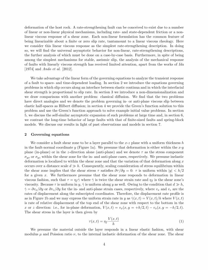
We consider a fault shear zone to be a layer parallel to the x-z plane with a uniform thickness hin the fault-normal coordinate y (Figure 1a). We presume that deformation is either within the x-yplane (in-plane) or in the z-direction alone (anti-plane) and we denote τ as the stress componentσyx or σyz within the shear zone for the in- and anti-plane cases, respectively. We presume inelasticdeformation is localized to within the shear zone and that the variation of that deformation along xoccurs over a distance scale d� h. Consequently, scaling consideration of stress equilibrium withinthe shear zone implies that the shear stress τ satisfies ∂τ/∂y = 0: τ is uniform within |y| < h/2for a given x. We furthermore presume that the shear zone responds to deformation in linearviscous fashion, such that τ = ηf γ where γ is twice the shear strain rate and ηf is the shear zone’sviscosity. Because τ is uniform in y, γ is uniform along y as well. Owing to the condition that d� h,γ = ∂vx/∂y or ∂vz/∂y for the in- and anti-plane strain cases, respectively, where vx and vz are therates of displacement along the subscripted coordinates. Therefore, the displacement rate profile isas in Figure 1b and we may express the uniform strain rate in y as γ(x, t) = V (x, t)/h where V (x, t)is rate of relative displacement of the top end of the shear zone with respect to the bottom in thex or z direction: i.e., for in-plane deformation, V (x, t) = vx(x, y = +h/2, t) − vx(x, y = −h/2, t).The shear stress in the layer is then given by

τ(x, t) = ηfV (x, t)

h(1)

We presume the material outside the layer responds in a linear elastic fashion, with shearmodulus µ and Poission ratio ν, to the internal inelastic deformation of the shear zone. The shear

4

u+x

u−x

δ(x, t)

x

y

h

µ, ν

ηf

u+x

u−x

δ(x, t)

x

y

µ, ν

ηf

τ(x, t)

(a) (b)

Figure 1: Illustration of model geometry and shear zone deformation. (a) A viscous shear zoneof thickness h and viscosity ηf lies between two linear elastic half-spaces of shear modulus µ andPoisson ratio ν. In-plane deformation of the shear zone is drawn, with the layer undergoing uniformstrain and a relative displacement δ = u+

x − u−x , where u+x and u−x denote the displacement of the

top and bottom faces of the shear zone. (b) Over distances much greater than h, the problem in(a) appears as two linear-elastic half-spaces in contact undergoing the relative displacement δ withthat motion being resisted by an interfacial shear stress τ .

traction along the elastic bodies’ boundaries at y = ±h/2 is identically τ , owed to the continuityof fault-normal tractions across the boundaries. We denote the relative displacement of the shearzone δ(x, t), such that V = ∂δ/∂t, and for the in-plane case δ(x, t) = ux(x, y = +h/2, t)−ux(x, y =−h/2, t), where ux is the displacement in the x direction. Given that we are concerned withvariations of deformation of the shear zone along x at scales d� h, we may effectively collapse theshear zone onto a fault plane along y = 0 and no longer give the layer explicit consideration. Dueto the quasi-static, elastic deformation of the material external to the shear zone, the distributionof τ along the fault surface (i.e., the surface formerly demarcated along y = ±h/2, and now alongy = 0±) must also satisfy

τ(x, t) =µ′

π

∫ ∞−∞

∂δ(s, t)/∂s

s− x ds+ τb(x, t) (2)

where µ′ = µ/[2(1− ν)] and µ′ = µ/2 for the in-plane and anti-plane cases, respectively. The lastterm on the right hand side is the shear tractions resolved on the fault plane due to external forcingwhile the first term is the change in shear tractions owed to a distribution of relative displacement,or slip, along the fault.

To draw useful comparisons later, we briefly consider here another configuration, one in which anelastic layer of thickness b� h lies above the shear zone, and an elastic half-space lies underneath.

5

In this case, when deformation along x occurs over distances much longer than b, τ is instead givenby [Viesca, 2016, supplementary materials]

τ(x, t) = E′b∂2δ(x, t)

∂x2+ τb(x, t) (3)

where E′ = 2µ/(1− ν) and E′ = µ for the in-plane and anti-plane cases.

Combining (1) with (2) or (3) results in an equation governing the spatio-temporal evolutionof slip δ. In the section that follows we first non-dimensionalize this equation and subsequentlyhighlight the diffusive nature of fault slip evolution.

3 Problem non-dimensionalization

Positing a characteristic slip rate Vc, we may in turn define characteristic values of shear stressτc = ηfVc/h, time tc = h/Vc, along-fault distance xc = µ′h/τc or xc =

√E′bh/τc, and slip δc = h.

We update our notation going forward to reflect the following nondimensionalization:

V/Vc ⇒ V, τb/τc ⇒ τb, t/tc ⇒ t, x/xc ⇒ x, and δ/δc ⇒ δ

Doing so, the combination of (1) with (2) leads to

∂δ

∂t= H

(∂δ

∂x

)+ τb(x, t) (4)

where we identify the operator H(f) = (1/π)∫∞−∞ f(s)/(s− x)ds on a spatial function f(x) as the

Hilbert transform. Useful properties of the Hilbert transform are that H[H(f)] = −f and that itcommutes with derivatives in time and space: e.g., d[H(f)]/dx = H[df/dx].

For comparison, if we similarly combine and and non-dimensionalize (1) with (3),

∂δ

∂t=

∂

∂x

(∂δ

∂x

)+ τb(x, t) (5)

we immediately recognize that slip rate in this case satisfies the diffusion equation, with an externalforcing term τb. While (5) is a classical problem with known solution, the dynamics of (4), incontrast, has remained without comparable study despite being the simplest formulation of a rate-strengthening fault within an elastic continuum and despite also being among the simplest non-local, diffusion-type equations. However, in the sections to follow we highlight that the linearity ofproblem (4), which we refer to as the Hilbert diffusion equation, makes it as amenable to solutionas the classical diffusion equation, though with several signature features.

4 Solution via Green’s function

We begin by looking for the fundamental solution, also known as the Green’s function, to theproblem in which the external forcing takes the form of an impulse in at position x′ and time t′,i.e., the function G(x, t;x′, t′) satisfying

∂G

∂t= H

(∂G

∂x

)+ δD(x− x′)δD(t− t′) (6)

6

–6 –4 –2 0 2 4 6x

0

0.2

0.4

0.6

0.8

V(x

;t)

t = 4

1/2

2

1

1/4

–5 –4 –3 –2 –1 0 1 2 3 4 5x=t

0

0.1

0.2

0.3

0.4

0.5

0.6

V(x

;t)

t

t = 1/4

1/2

1

4

:

(a) (b)

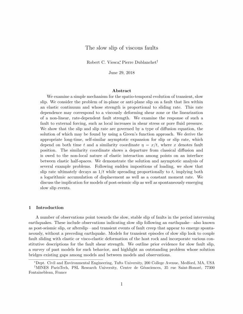
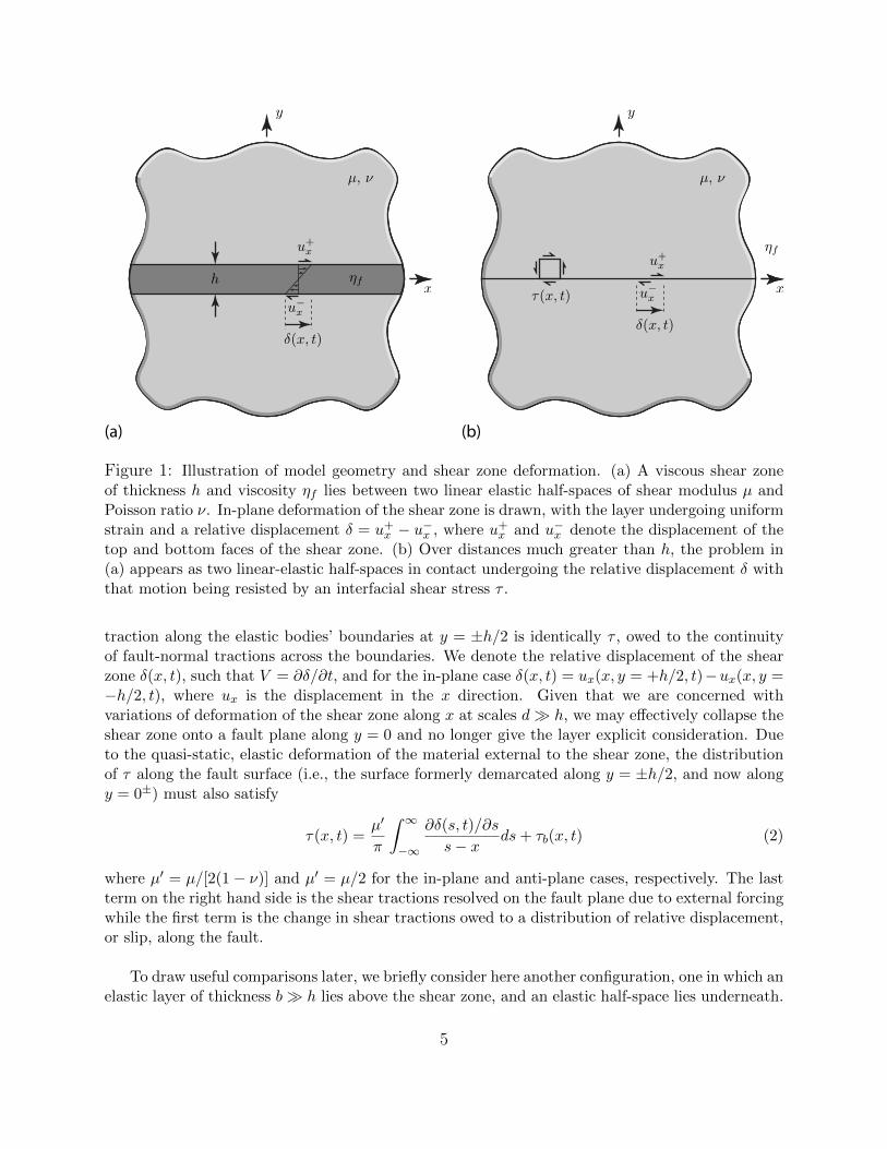
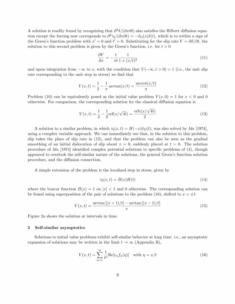
Figure 2: (a) Solutions for slip rate at intervals of time t following an initial step in stress at t = 0with a boxcar spatial distribution about x = 0. (b) Rescaling of the solutions in (a) to highlightthe approach to the leading-order self-similar asymptotic solution (blue).

where we denote the Dirac delta function as δD(x). Following standard techniques (outlined inAppendix A), the Green’s function for the Hilbert diffusion equation is, for t > t′

G(x, t;x′, t′) =1

π(t− t′)1

1 +

(x− x′t− t′

)2 (7)

The Green’s function exhibits self-similar behavior, in which distances x stretch with time t. Whilenot explicitly considered as such, the Green’s function solution was effectively also derived by Ida[1974] and Ando et al. [2012]. To contrast, we recall that the Green’s function solution for classicaldiffusion is

G(x, t;x′, t′) =1√

4π(t− t′)exp

[−(x− x′)2

4(t− t′)

](8)

in which the power-law decay of the the Lorentzian 1/[π(1+s2)] gives way to the exponential decayof a Gaussian and now distance x stretches with

√t. This latter change could be anticipated from

scaling of the equations (4) and (5), excluding the source term, in which we find that [D]/[T] ∼[D]/[L] in (4) and [D]/[T] ∼ [D]/[L2] in (5), where the scalings of slip, time, or length are denotedby [D], [T], and [L], respectively.

Solutions to the problem of an arbitrary external forcing τb(x, t) are given by the convolution[e.g., Carrier and Pearson, 1976]

δ(x, t) =

∫ ∞−∞

∫ t

−∞G(x, t;x′, t′)τb(x

′, t′)dt′dx′ (9)

4.1 Example: Sudden step in stress

As a simple example we consider the problem in which a sudden step in stress of unit magnitudeis applied at t = 0 and along x < 0, or

τb(x, t) = H(−x)H(t) (10)

7

A solution is readily found by recognizing that ∂2δ/(∂x∂t) also satisfies the Hilbert diffusion equa-tion except the forcing now corresponds to ∂2τb/(∂x∂t) = −δD(x)δ(t), which is to within a sign ofthe Green’s function problem with x′ = 0 and t′ = 0. Substituting for the slip rate V = ∂δ/∂t, thesolution to this second problem is given by the Green’s function, i.e. for t > 0

∂V

∂x= − 1

πt

1

1 + (x/t)2(11)

and upon integration from −∞ to x, with the condition that V (−∞, t > 0) = 1 (i.e., the unit sliprate corresponding to the unit step in stress) we find that

V (x, t) =1

2− 1

πarctan(x/t) =

arccot(x/t)

π(12)

Problem (10) can be equivalently posed as the initial value problem V (x, 0) = 1 for x < 0 and 0otherwise. For comparison, the corresponding solution for the classical diffusion equation is

V (x, t) =1

2− 1

2erf(x/

√4t) =

erfc(x/√

4t)

2(13)

A solution to a similar problem, in which τb(x, t) = H(−x)δD(t), was also solved by Ida [1974],using a complex variable approach. We can immediately see that, in the solution to this problem,slip takes the place of slip rate in (12), and that the problem can also be seen as the gradualsmoothing of an initial dislocation of slip about x = 0, suddenly placed at t = 0. The solutionprocedure of Ida [1974] identified complex potential solutions to specific problems of (4), thoughappeared to overlook the self-similar nature of the solutions, the general Green’s function solutionprocedure, and the diffusion connection.

A simple extension of the problem is the localized step in stress, given by

τb(x, t) = B(x)H(t) (14)

where the boxcar function B(x) = 1 on |x| < 1 and 0 otherwise. The corresponding solution canbe found using superposition of the pair of solutions to the problem (10), shifted to x = ±1

V (x, t) =arctan [(x+ 1)/t]− arctan [(x− 1)/t]

π(15)

Figure 2a shows the solution at intervals in time.

5 Self-similar asymptotics

Solutions to initial value problems exhibit self-similar behavior at long time: i.e., an asymptoticexpansion of solutions may be written in the limit t→∞ (Appendix B),

V (x, t) =

∞∑n=1

1

tnRe[cnfn(η)] with η = x/t (16)

8

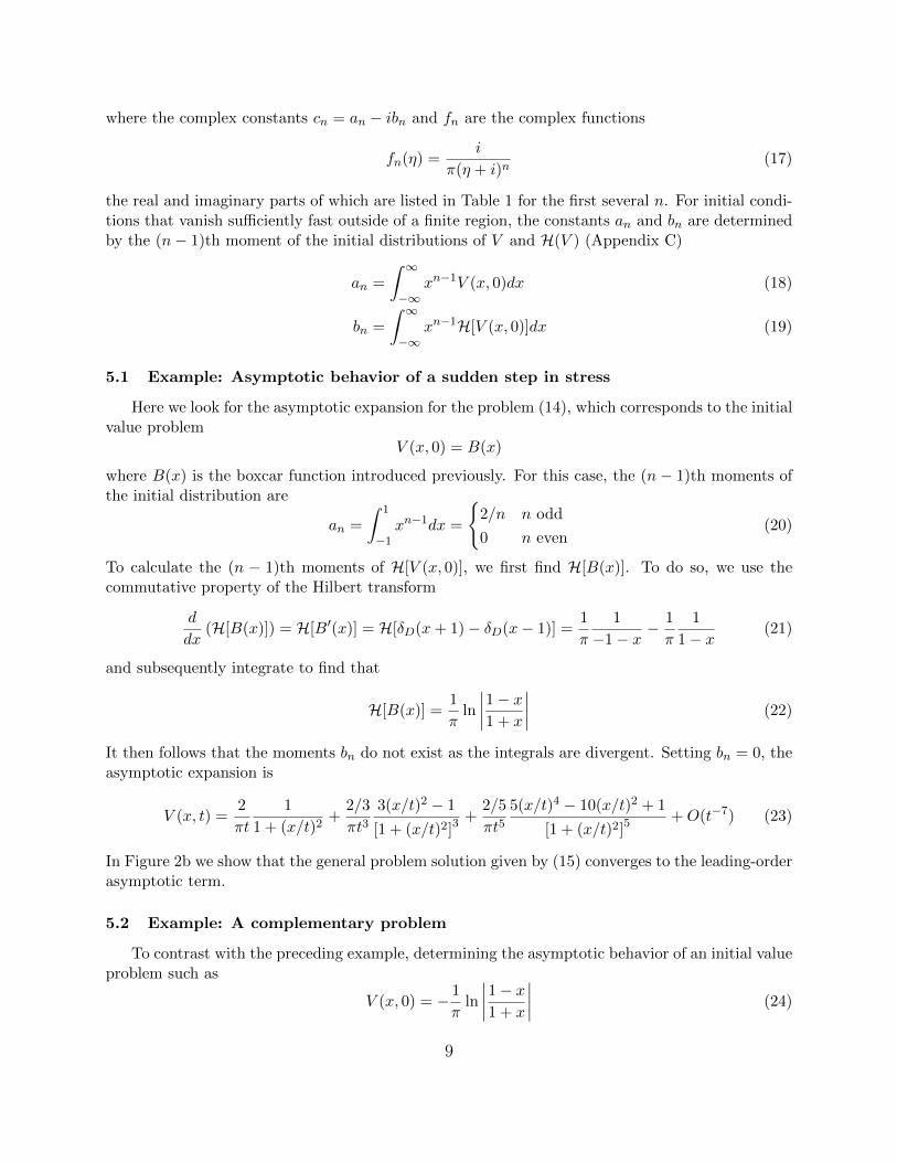
where the complex constants cn = an − ibn and fn are the complex functions

fn(η) =i

π(η + i)n(17)

the real and imaginary parts of which are listed in Table 1 for the first several n. For initial condi-tions that vanish sufficiently fast outside of a finite region, the constants an and bn are determinedby the (n− 1)th moment of the initial distributions of V and H(V ) (Appendix C)

an =

∫ ∞−∞

xn−1V (x, 0)dx (18)

bn =

∫ ∞−∞

xn−1H[V (x, 0)]dx (19)

5.1 Example: Asymptotic behavior of a sudden step in stress

Here we look for the asymptotic expansion for the problem (14), which corresponds to the initialvalue problem

V (x, 0) = B(x)

where B(x) is the boxcar function introduced previously. For this case, the (n− 1)th moments ofthe initial distribution are

an =

∫ 1

−1xn−1dx =

{2/n n odd

0 n even(20)

To calculate the (n − 1)th moments of H[V (x, 0)], we first find H[B(x)]. To do so, we use thecommutative property of the Hilbert transform

d

dx(H[B(x)]) = H[B′(x)] = H[δD(x+ 1)− δD(x− 1)] =

1

π

1

−1− x −1

π

1

1− x (21)

and subsequently integrate to find that

H[B(x)] =1

πln

∣∣∣∣1− x1 + x

∣∣∣∣ (22)

It then follows that the moments bn do not exist as the integrals are divergent. Setting bn = 0, theasymptotic expansion is

V (x, t) =2

πt

1

1 + (x/t)2+

2/3

πt33(x/t)2 − 1

[1 + (x/t)2]3+

2/5

πt55(x/t)4 − 10(x/t)2 + 1

[1 + (x/t)2]5+O(t−7) (23)

In Figure 2b we show that the general problem solution given by (15) converges to the leading-orderasymptotic term.

5.2 Example: A complementary problem

To contrast with the preceding example, determining the asymptotic behavior of an initial valueproblem such as

V (x, 0) = − 1

πln

∣∣∣∣1− x1 + x

∣∣∣∣ (24)

9

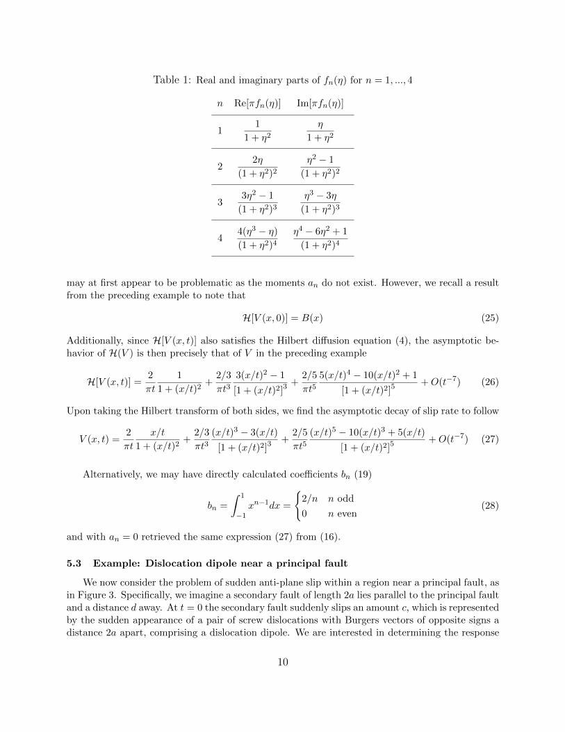
Table 1: Real and imaginary parts of fn(η) for n = 1, ..., 4

n Re[πfn(η)] Im[πfn(η)]

11

1 + η2

η

1 + η2

22η

(1 + η2)2

η2 − 1

(1 + η2)2

33η2 − 1

(1 + η2)3

η3 − 3η

(1 + η2)3

44(η3 − η)

(1 + η2)4

η4 − 6η2 + 1

(1 + η2)4

may at first appear to be problematic as the moments an do not exist. However, we recall a resultfrom the preceding example to note that

H[V (x, 0)] = B(x) (25)

Additionally, since H[V (x, t)] also satisfies the Hilbert diffusion equation (4), the asymptotic be-havior of H(V ) is then precisely that of V in the preceding example

H[V (x, t)] =2

πt

1

1 + (x/t)2+

2/3

πt33(x/t)2 − 1

[1 + (x/t)2]3+

2/5

πt55(x/t)4 − 10(x/t)2 + 1

[1 + (x/t)2]5+O(t−7) (26)

Upon taking the Hilbert transform of both sides, we find the asymptotic decay of slip rate to follow

V (x, t) =2

πt

x/t

1 + (x/t)2+

2/3

πt3(x/t)3 − 3(x/t)

[1 + (x/t)2]3+

2/5

πt5(x/t)5 − 10(x/t)3 + 5(x/t)

[1 + (x/t)2]5+O(t−7) (27)

Alternatively, we may have directly calculated coefficients bn (19)

bn =

∫ 1

−1xn−1dx =

{2/n n odd

0 n even(28)

and with an = 0 retrieved the same expression (27) from (16).

5.3 Example: Dislocation dipole near a principal fault

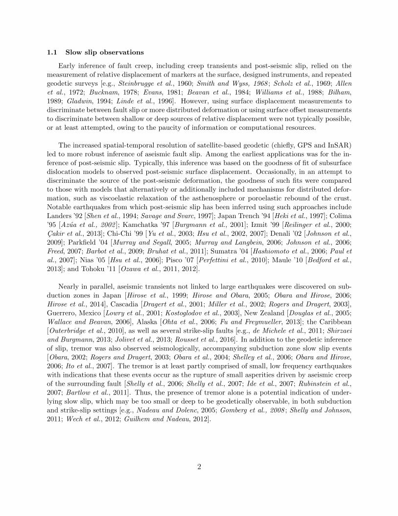
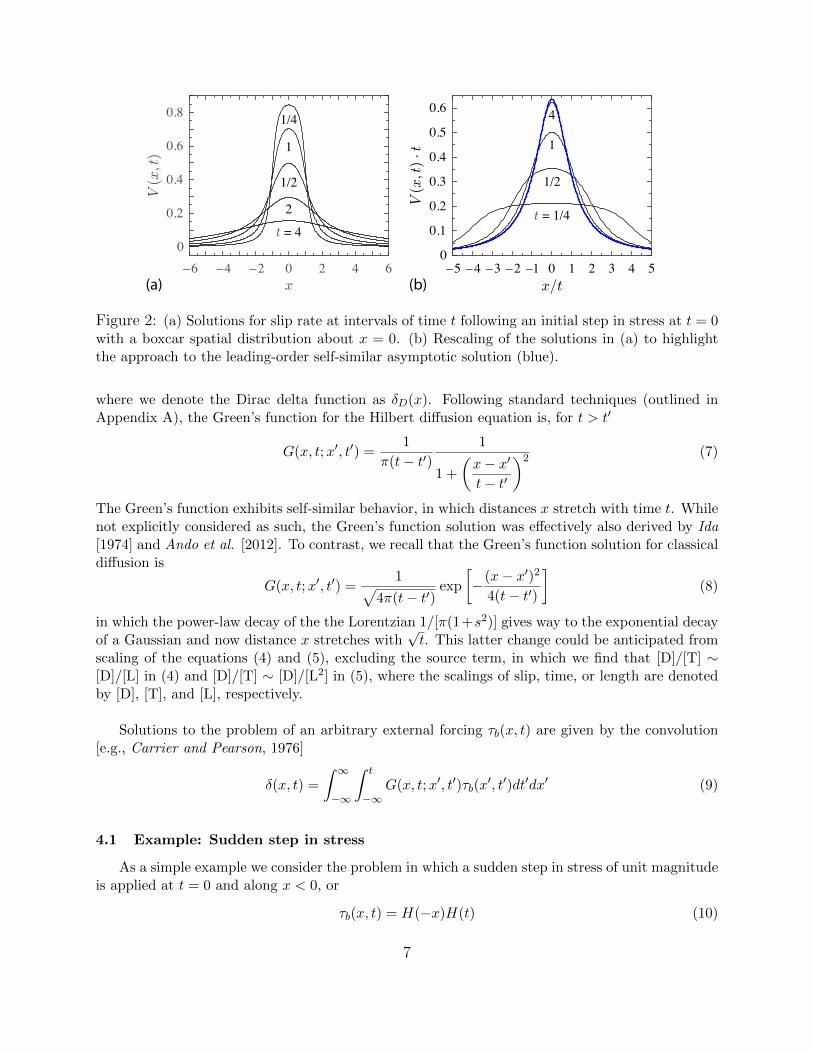
We now consider the problem of sudden anti-plane slip within a region near a principal fault, asin Figure 3. Specifically, we imagine a secondary fault of length 2a lies parallel to the principal faultand a distance d away. At t = 0 the secondary fault suddenly slips an amount c, which is representedby the sudden appearance of a pair of screw dislocations with Burgers vectors of opposite signs adistance 2a apart, comprising a dislocation dipole. We are interested in determining the response

10

x

y

x

δs(x ) = u+z − u−

z

d 2a

c

Figure 3: Illustration of the model problem considered in sub-section 5.3, a relatively small sec-ondary fault undergoes an amount c of relative anti-plane displacement δs at t = 0. The secondaryfault has a width 2a and is located a distance d away from the principal fault, which lies along thex− z plane.

of the principal fault to this perturbation. The off-fault dislocation dipole induce the stress changeon the principal fault of the form

τb(x, t) =c

π

[x− a

d2 + (x− a)2− x+ a

d2 + (x+ a)2

]H(t) (29)

We may alternatively consider the posed problem as an initial value problem for the anti-plane sliprate of the principal fault

V (x, 0) =c

π

[x− a

d2 + (x− a)2− x+ a

d2 + (x+ a)2

](30)

One path to the full solution is to recognize that the function h(x, t) = H[V (x, t)] also satisfiesthe Hilbert diffusion equation. We may now pose the problem as an inital value problem for h(x, t)where

h(x, 0) = H[V (x, 0)] =c

π

[d

d2 + (x− a)2− d

d2 + (x+ a)2

](31)

Recognizing the form of the Green’s function, the solution of the auxiliary problem is, by inspection,

h(x, t) =c

π(t+ d)

[1

1 + [(x− a)/(t+ d)]2− 1

1 + [(x+ a)/(t+ d)]2

](32)

The solution to the original problem then follows from the inversion for V (x, t) = −H[h(x, t)]

V (x, t) =c

π(t+ d)

[(x− a)/(t+ d)

1 + [(x− a)/(t+ d)]2− (x+ a)/(t+ d)

1 + [(x+ a)/(t+ d)]2

](33)

11

where in the above we used the known transform H[x/(b2 + x2)] = b/(b2 + x2) for b a constant inspace and the property that H{H[f(x)]} = −f(x).

To find the asymptotic behavior, we look to determine the coefficients of the expansion, anand bn. However, this example is unlike the preceding ones owing to the power-law decay of boththe initial slip rate and its Hilbert transform. Consequently, the moment integral expressions foran and bn as written in (18) and (19) are divergent for n sufficiently large. Nonetheless, we mayproceed to determine the coefficients as follows.

First, given the problem symmetry, V (x, t) = V (−x, t), we may anticipate that an = 0 when nis even and bn = 0 when n is odd as we expect to keep only functions that are symmetric aboutx = 0 in the asymptotic expansion. Proceeding to determine the moments of the initial distributionand its Hilbert transform, leads to a1 = 0 and b2 = 2ac, the last of which we identify as the netmoment of the dislocation dipole

mo = 2ac

Examining the next-order moment a3, we find that the integral is divergent. This divergence isowed to the integrand approaching a finite value as x→ ±∞:

limx→±∞

x2V (x, 0) =mo

π

Subtracting this limit value from the integrand when calculating the moment, we find

a3 =

∫ ∞−∞

[x2V (x, 0)− mo

π

]dx = −mo(2d)

The integrand of the moment b4 likewise diverges due to the integrand having a non-zero limit inthe far-field

limx→±∞

x3H[V (x, 0)] = −mo(2d)

π

Proceeding similarly, we find that

b4 =

∫ ∞−∞

[x3H[V (x, 0)] +

mo(2d)

π

]dx = mo(a

2 − 3d2)

To determine the next-order coefficient a5, we note that as x→∞

x4V (x, 0) ≈ x2mo

π+mo(a

2 − 3d2)

π+O(x−2)

the first two terms of which preclude the moment integral from being convergent. Subtracting theseterms from the moment integrand, we arrive to

a5 =

∫ ∞−∞

[x4V (x, 0)− x2mo

π− mo(a

2 − 3d2)

π

]dx = mo[4d(d2 − a2)]

12

Thus, the four leading-order terms in the asymptotic expansion are

V (x, t) =mo

πt2(x/t)2 − 1

[1 + (x/t)2]2− mo(2d)

πt33(x/t)2 − 1

[1 + (x/t)2]3+mo(a

2 − 3d2)

πt4(x/t)4 − 6(x/t)2 + 1

[1 + (x/t)2]4

+mo[4d(d2 − a2)]

πt55(x/t)4 − 10(x/t)2 + 1

[1 + (x/t)2]5+O(t−7) (34)

We emphasize that the leading term is independent of the distance d and dependent on a and conly insofar as they determine the dipole moment mo. Subsequent terms are found following theprocedure outlined above, i.e., given that a1 = 0 and b2 = mo

an =

∫ ∞−∞

xn−1V (x, 0)− 1

π

(n−1)/2∑k=1

x(n−1)−2k b2k

dx for n = 3, 5, 7, ... (35)

bn =

∫ ∞−∞

xn−1H[V (x, 0)]− 1

π

(n−2)/2∑k=1

x(n−2)−2k a2k+1

dx for n = 4, 6, 8, ... (36)

6 Comparison with spring-block and finite-fault models

In the preceding section we found that the asymptotic response to a stress step is a power-lawdecay in slip rate with time. In this section we highlight that such power-law decay transitions toexponential decay in time if locked fault boundaries are encountered. This transition to a morerapidly decaying slip rate is owed to limitations of the compliance of the coupled fault-host rocksystem. We begin by considering a simple system with a limited compliance: a sliding blockattached to a spring with fixed stiffness, finding the exponential decay of slip rate following a stepin stress. We subsequently examine a continuum system with limited compliance: a finite faultembedded within a full space. We examine the response of such a fault to a step in stress and showthat the decay of slip rate is expressible as the sum of orthogonal modes whose amplitudes have anexponential decay with time. We also highlight that the conditions for such asymptotic behavior arerather strict, requiring slip not penetrate beyond a particular position, and that non-exponentialdecay can be expected if fault boundaries are modeled as transitions in fault rheology.

6.1 Spring-block model

We consider a rigid block sliding on a rigid substrate. The block is attached to one end ofa spring, with stiffness k, the other end of which is attached to a pulled at a constant rate Vp.The basal shear stress is denoted τ and τb is the shear stress applied to the top of the block. Forquasi-static deformation,

τ(t) = k[Vpt− δ(t)] + τb(t) (37)

where δ(t) is both the basal slip and the displacement of the block. As before, we presume thebasal interface is modeled as a thin viscous layer such that the interfacial shear strength is

τs(t) = ηV (t)

h(38)

13

We consider the response to a sudden step in applied stress at t = 0

τb(t) = ∆τH(t) (39)

With the initial condition δ(0) = 0, the block’s displacement relative to the load point is given by

δ(t)− Vpt = (A−B)[1− exp(−t/tc)] (40)

where tc = η/(hk), A = ∆τ/k, and B = Vptc

6.2 Finite-fault model

We now consider the in-plane or anti-plane slip of a fault with a finite length 2L. The dimen-sional shear stress on the fault plane is given by.

τ(x, t) =µ′

π

∫ L

−L

∂δ(s, t)/∂s

s− x ds+ τb(x, t) (41)

with the condition that there is no slip for |x| > L, including the endpoints: δ(±L, t) = 0.

Nondimensionalizing as done previously to arrive to (4),

τ(x, t) =1

π

∫ L

−L

∂δ(s, t)/∂s

s− x ds+ τb(x, t) (42)

where the dimensionless fault length is denoted L = L/xc. Requiring that τ = τs within the faultplane |x| < L, the time rate of the above is

∂V (x, t)

∂t=

1

π

∫ L

−L

∂V (s, t)/∂s

s− x ds+∂τb(x, t)

∂t(43)

with the condition that V (±L, t) = 0.

We now look to determine how the finite fault responds to a step in stress τb(x, t) = f(x)H(t).We may alternatively pose this problem as the initial value problem for the slip rate as V (x, 0) =f(x) where the slip rate for t > 0 satisfies

∂V (x, t)

∂t=

1

π

∫ L

−L

∂V (s, t)/∂s

s− x ds (44)

We begin by looking for solutions to (44) of the form

V (x, t) = ω(x/L) exp(λt/L) (45)

which, when substituted into (44) leads to the eigenvalue problem

λω(x) =1

π

∫ 1

−1

dω(s)/ds

s− x ds (46)

14

previously analyzed in the context of earthquake nucleation on linearly slip-weakening faults [Das-calu et al., 2000 ; Uenishi and Rice, 2003]. As discussed by those authors, solutions to the eigenequation have the following properties: the eigenmodes ωn are orthogonal and correspond to a setof discrete, unique eigenvalues λn < 0, which can be arranged in decreasing order 0 > λ1 > λ2... .Consequently, the initial velocity distribution can be decomposed into a sum of the eigenfunctions

V (x, 0) =∞∑n=1

vnωn(x/L) (47)

where, owing to the orthogonality of ωn, the coefficients of the expansion are given by

vn =

∫ 1

−1V (sL, 0)ωn(s)ds∫ 1

−1ω2n(s)ds

(48)

and consequently, the solution to the initial value problem is

V (x, t) =∞∑n=1

vnωn(x/L) exp(λnt/L) (49)

The most slowly decaying symmetric and anti-symmetric modes can be accurately approximated,to within 1% besides an arbitrary scale factor, as

ω1(x) ≈√

1− x2(1− x2/3) (50)

ω2(x) ≈√

1− x2[1− (4x/5)2]x (51)

and have the eigenvalues λ1 = 0.578887... and λ2 = 1.377377... . The eigenfunctions and eigenvaluesmay be solved for numerically, as done by Dascalu et al [2000] using a Chebyshev polynomialexpansion, Uenishi and Rice [2000] using a discrete dislocation technique, or Brantut and Viesca[2015] using Gauss-Chebyshev-type quadrature for a comparable problem. Doing so, (48) and(49) are then readily evaluated numerically. The eigenfunction expansion can also be used toconstruct a Green’s function solution to the problem (42) or (43) with τb or ∂τb/∂t being equal toδ(x− x′)δ(t− t′), which we defer to later work.

7 Discussion

7.1 Relation with existing spring-block and continuum models for postseismic slip

Observations of surface displacements that appear to increase logarithmically with time havebeen used as evidence for postseismic deformation due to frictional afterslip or ductile deformationof faults, in part owed to the observation that such a logarithmic time dependence arises in modelsof stable fault slip. Early models have focused on the displacement response of spring-block systemsto steps in stress [e.g., Marone et al. 1991; Perfettini and Avouac, 2004; Montesi, 2004; Helmstetterand Shaw, 2009]. However, spring-block models in which the frictional strength linearizes abouta finite or zero value of slip rate—including slip rate- and state-dependent friction—all exhibit aslip rate that ultimately relaxes back to a zero or finite value exponentially with time following

15

a step in stress under a negligible or finite value of the load-point velocity Vp. Nonetheless, alogarithmic growth of displacement can arise from a spring-block model in some limiting caseswhen considering a frictional formulation that does not linearize about V = 0, specifically a strengthrelation τs(V ) = τo + c ln(V ). Revisiting the analysis of section 6.1 for the response of a spring-block system to a sudden step in stress and replacing the linear viscous strength relation with thislogarithmic slip-rate dependence, one finds that the asymptotic behavior is V ∼ 1/t, and henceδ ∼ ln(t), provided that the load point velocity Vp = 0. For finite values of Vp, the slip rateapproaches a 1/t decay only as an intermediate asymptote at sufficiently short times after the step,followed by a transition to an exponential decay of slip rate to the finite value of Vp at long time.

That strength may depend on the logarithm of slip rate is consistent with experimental ob-servations and the constitutive formulation for rate- and state-dependent friction insofar as theseboth exhibit a logarithmic dependence under steady-sliding conditions [Dieterich, 1978, 1979; Ru-ina, 1980, 1983]. Considering the full rate- and state-dependence, with aging-law state evolution,does not qualitatively change the behavior following a step in stress applied to a spring-blocksystem in comparison with a strictly logarithmic dependence on slip rate: a 1/t decay shortly af-ter the step transitions to oscillatory exponential decay at long time [e.g., Rice and Ruina, 1983;Helmstetter and Shaw, 2009]. This has made the spring-block model a common representationof post-seismic fault slip when attempting to fit observed displacements with the functional formδ(t) = δc ln(1 + t/tc), and the goodness of fit has furthermore been taken as evidence in support ofa rate- and state-dependent description governing fault strength in the post-seismic period. Specif-ically, the spring-block model of Marone et al. [1991] is based on the strict logarithmic dependenceand Vp = 0, while Perfettini and Avouac [2004] relax the latter assumption and Helmstetter andShaw [2009] consider the full rate- and state-dependent formulation and show the limiting caseswhere a 1/t decay in slip rate may arise.

However, we find here that a logarithmic dependence of fault displacement with time alsoemerges from a fault with a simple linear viscous strength when including the interactions betweenpoints on the fault that accompany a continuum description, which is neglected in spring blockmodels. Specifically, the asymptotic expansion for slip rate (16) given a step in stress on the faultat the leading order has a1 6= 0 and b1 = 0, which, upon integration, provides the asymptotic formof fault slip

δ(x, t) =a1

πln(x2 + t2

)+O

(t−1)

(52)

the long-time behavior of which, for fixed x and long time, is indistinguishable from a functionalfit of the form δ(t) = ln(1 + t), when a1 = π/2 (and bearing in mind that δ and t are dimensionlessquantities here, in which the subsumed slip and time scales δc and tc are presumed to remain asfitting parameters). Moreover, any rate-strengthening rheology that linearizes about a finite or zeroslip rate, will have the same asymptotic behavior as the linear viscous fault, to leading order. Thisuniversal asymptotic behavior poses an obstacle to discriminate among different rate-strengtheningfault rheological descriptions on the basis of displacement data at long times. Nonetheless, theuniversal behavior does provide a long-time signature of stable fault slip following a step in stress,if not the capability of identifying a specific mechanism for that stable response other than arate-strengthening fault rheology.

16

x

yτb(x, 0+) y

x

τb(x, 0+)

u+z (x, t)u−

z (x, t)

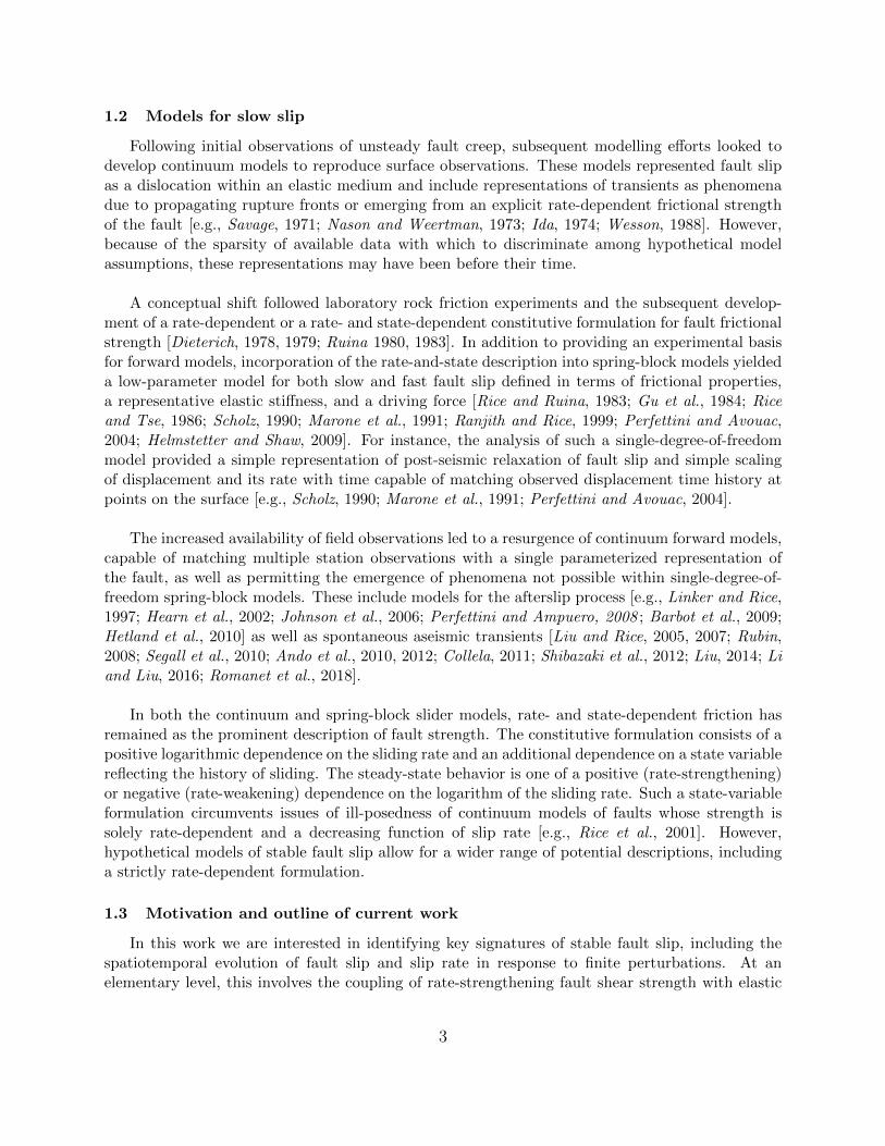
Figure 4: An anti-plane fault in the x-z plane intersects a free surface at x = 0. The solution to asudden step in stress τb at t = 0+ along the fault (x > 0) is found by method of images. The imageproblem is shown as a transparent continuation.

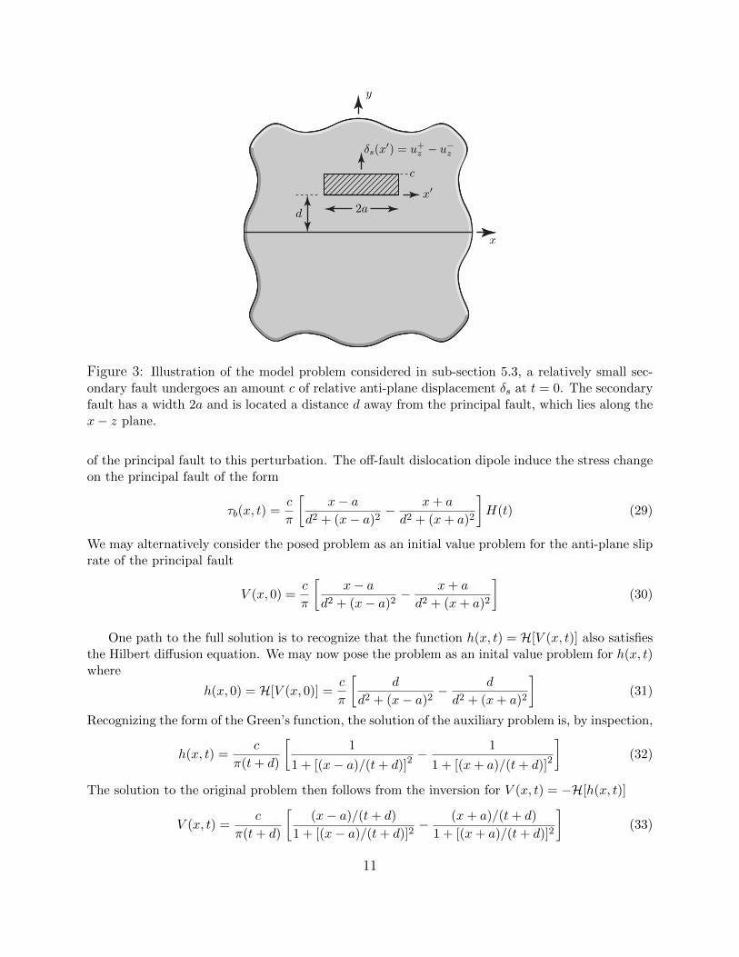
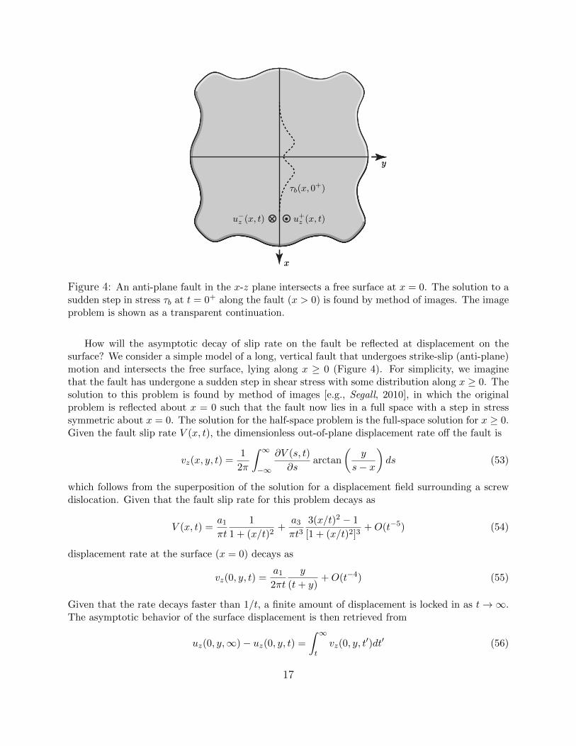
How will the asymptotic decay of slip rate on the fault be reflected at displacement on thesurface? We consider a simple model of a long, vertical fault that undergoes strike-slip (anti-plane)motion and intersects the free surface, lying along x ≥ 0 (Figure 4). For simplicity, we imaginethat the fault has undergone a sudden step in shear stress with some distribution along x ≥ 0. Thesolution to this problem is found by method of images [e.g., Segall, 2010], in which the originalproblem is reflected about x = 0 such that the fault now lies in a full space with a step in stresssymmetric about x = 0. The solution for the half-space problem is the full-space solution for x ≥ 0.Given the fault slip rate V (x, t), the dimensionless out-of-plane displacement rate off the fault is

vz(x, y, t) =1

2π

∫ ∞−∞

∂V (s, t)

∂sarctan

(y

s− x

)ds (53)

which follows from the superposition of the solution for a displacement field surrounding a screwdislocation. Given that the fault slip rate for this problem decays as

V (x, t) =a1

πt

1

1 + (x/t)2+

a3

πt33(x/t)2 − 1

[1 + (x/t)2]3+O(t−5) (54)

displacement rate at the surface (x = 0) decays as

vz(0, y, t) =a1

2πt

y

(t+ y)+O(t−4) (55)

Given that the rate decays faster than 1/t, a finite amount of displacement is locked in as t→∞.The asymptotic behavior of the surface displacement is then retrieved from

uz(0, y,∞)− uz(0, y, t) =

∫ ∞t

vz(0, y, t′)dt′ (56)

17

Denoting the long-term displacement uz(0, y,∞) = u∞z , the displacement evolution towards thisvalue is found by substituting for vz in the above, and to leading order

uz(0, y, t) = u∞z −a1

2πln

(t+ y

t

)(57)

which has the short- and long-time behavior, respectively

uz(0, y, t) = u∞z +a1

2πln(t/y) (58)

uz(0, y, t) = u∞z −a1

2π

y

t(59)

the first of which suggests that the apparent logarithmic growth observed in field measurementsof surface displacements may be an intermediate asymptotic that ultimately saturates if there is anegligible far-field loading rate.

To clearly outline the interplay between continuum deformation and fault rheology and tohighlight its consistency with observations, we have thus far considered relatively simple modelgeometries; however, an extensive effort of using forward models of frictional faults embeddedin a continuum to account for geodetic afterslip observations has accompanied both the increasein GPS data and computational resources needed to run many iterations of the forward modelsfor parameter inversion. Linker and Rice [1997] sought to reproduce the observed postseismicdeformation following the Loma Prieta earthquake, considering several model fault geometrieswhile comparing the response to a sudden step in stress of a linear viscoelastic fault rheology witha so-called hot-friction model, τ ∼ lnV , intended to mimic the steady-state behavior of rate- andstate-dependent friction. Both models provided comparable fits to the surficial displacements, withthe conclusion that while deep relaxation process may be adequate, discriminating among differentrheological models remains an issue. This continued to be reflected in subsequent efforts, includingthat of Hearn et al. [2002], who considered geodetic observations of postseismic deformation inresponse to the 1999 Izmit earthquake. The authors performed a parameter inversion using aforward model to determine whether postseismic deformation in response to a co-seismic step inshear stress arises by viscoelastic relaxation of the lower crust, poroelastic rebound, or via a faultslip on regions at depth whose strength obeys a linear viscous strength of the type examinedhere or the logarithmic hot-friction model also used in Linker and Rice [1997] and Marone et al.[1991]. While poroelastic rebound was quickly ruled out and the frictional afterslip models offeredimprovements over the strictly viscoelastic model, the discrepancies between fault models withlinear and logarithmic slip-rate dependence were marginal.

That different frictional models may have consistent asymptotic behavior is further supportedwhen considering numerical studies of stable afterslip. Hetland et al. [2010] examined numericalsolutions for the post-seismic response to imposed co-seismic stress changes on vertical strike-slip(anti-plane) faults that obeyed a wide range of frictional constitutive relations, ranging from linearand power-law non-linear viscous to logarithmic hot friction and rate- and state-dependence. Theauthors focus on the latter two relations and the numerical results show that the long-time decay ofslip rates at a fixed position follow the expected 1/t decay anticipated by our analytical treatmenthere, given that the models examined are expected to relax back to the finite, model-driving sliprate about which these non-linear constitutive relations can be linearized. Our expected 1/t decay,

18

as well as a spatial spreading of elevated slip rates that is proportional to time, is also reflected inseveral other numerical studies of rate-strengthening faults [e.g., Ariyoshi et al., 2007; Perfettiniand Ampuero, 2008]

While the issue of determining the relative contributions of different mechanisms to postseismicdeformation remains, cases in which afterslip appears to be the dominant mechanism [e.g., Freed,2007] do appear to be well modeled as the accelerated creep of a fault with a rate- (and possiblystate-) dependent friction [e.g., Johnson et al., 2006; Barbot et al., 2009 ]; however, such studiesfocus on a single fault strength description or rheology and comparatively little effort has beenmade to determine whether a particular rate-strengthening rheology is called for among severalplausible ones [Montesi, 2004]. That disparate, non-linear rheological relations may share a commonasymptotic behavior indicates that such an effort to discriminate requires careful attention.

7.2 Moment-duration scalings of spontaneous slow slip events

Another potential observational constraint on fault strength follows from slow slip events onsubduction faults that occur without the accompaniment of a large earthquake. These eventswere first observed geodetically [Hirose et al., 1999; Dragert et al., 2001] and subsequently foundto be accompanied by seismic tremor [Rogers and Dragert, 2003; Obara et al., 2004; Obara andHirose, 2006). Compiled estimates of moment release and duration of subduction zone slow slipevents appear to show a linear relationship between these quantities [Schwartz and Rokoksky, 2007;Ide et al., 2007; Aguiar et al., 2009 ; Gao et al., 2012; Liu, 2014]. Slow slip events were shown toemerge spontaneously from fault models with slip rate- and state-dependent friction under marginalconditions for frictional instability [Liu and Rice, 2005, 2007; Rubin, 2008]. Such numerical modelsare capable of producing a range of event sizes with a moment-duration relation that is arguablylinear [Shibazaki et al., 2012; Liu, 2014; Li and Liu, 2016; Romanet et al., 2018]; however, amechanistic explanation for the emergence of such a scaling has been missing, making it difficultto assess the robustness of and the necessary conditions for the observed model scaling.

Here we highlight alternative conditions permitting the existence of slow slip and show that alinear moment-duration scaling arises naturally from the stable response of a rate-strengtheningfault to a stress perturbation or sudden elevation of pore fluid pressure. For simplicity, we focuson the example of a fault undergoing in-plane or anti-plane rupture, in which slip varies only alongone dimension; however, the same conclusion can be reached following a similar line of argumentgiven comparable slip-rate self-similarity on a fault undergoing mixed-mode rupture, in which slipvaries in two dimensions.

For a fault in which slip varies along one dimension, the moment per unit fault thickness in theout-of-plane direction is defined as

M(t) = µ

∫ ∞−∞

δ(x, t)dx (60)

and the moment rate is, using dot notation to denote a derivative with respect to time,

M(t) = µ

∫ ∞−∞

V (x, t)dx (61)

19

where in the two equations above we have momentarily returned to using dimensional variables.We now pass to non-dimensional variables as done to arrive to (4) and for the moment and momentrates using M(t)/(µδcxc)⇒M(t) and M(t)/(µVcxc)⇒ M(t). We are interested in the asymptoticevolution of the fault moment release with time duration t following a step in stress. Substitutingthe asymptotic expression for fault slip rate following a step in stress (54), we find that the momentrate to leading order is constant, i.e.,

M(t) =a1

πt

∫ ∞−∞

1

1 + (x/t)2dx = a1 (62)

The constant a1 can be interpreted as the net increase of force on the fault, per unit out-of-planefault thickness, owed to the distributed stress step: i.e., for a stress step in the form τb(x, t) =∆τ(x)H(t)

a1 =

∫ ∞−∞

∆τ(x)dx (63)

This representation is seen by recognizing that the integral defining a1

a1 =

∫ ∞−∞

V (x, 0)dx (64)

directly follows, given the relation τ = V , from the more general statement of conservation fort > 0

a1 =

∫ ∞−∞

τ(x, t)dx (65)

which is itself deduced by demonstrating that, for t > 0

d

dt

∫ ∞−∞

τ(x, t)dx = 0 (66)

by substituting the expression (4) for the fault shear stress τ , recognizing that ∂[H(∂δ/∂x)]/∂t =∂H(V )/∂x, and using the condition that H(V ) vanishes at x = ±∞. This implies that, for t > 0

a1 =

∫ ∞−∞

τb(x, t)dx (67)

from which (63) follows.

The above conservation condition on the net shear force exerted on the fault by the shear stresschange, which implied a constant moment rate, is independent of the fault elastic configurationand mode of slip. In other words, while we considered the particular case of in- or anti-plane slipbetween elastic half-spaces, a constant moment rate would also be expected for any configuration—including mixed-mode slip between elastic half-spaces, or in proximity to a free surface—in whichthe fault strength is proportional to the sliding rate. By corollary, this also implies that a constantmoment rate would ultimately be expected for non-linear, rate-dependent (and rate-strengthening)descriptions of fault strength, which can be considered to approach an effective linear-viscousresponse as the fault relaxes back to a steady sliding velocity.

20

While we have thus far shown that the moment release following a step in stress is asymptoticallylinear in time, we have not yet identified potential mechanisms for such a step that would initiate aslow slip event. While there may be potential causes for a fault to experience an increase in shearstress, we briefly outline here conditions by which an increase in pore fluid pressure could lead to aslow slip event with a linear moment-duration relationship. Specifically, we assume fault strengthis frictional in nature and rate-strengthening with the simple form f(V ) = fo + cV , where hereand in what follows we continue the dimensionless representation for brevity. The frictional natureof the strength implies that the shear strength can be written as τs = σf where σ is the effectivenormal stress σ = σ − p, the difference between the total fault-normal stress σ and the fault porefluid pressure p. We consider a sudden increase in pore fluid pressure beyond an initial value po ofthe form p(x, t) = po + ∆p(x)H(t), where we neglect here details of the fluid pressure evolution,but simply assume the rise time is short and the distribution is compact in space. The requirementthat τs = τ when and where sliding occurs can then be rearranged to have a form comparable tothat of a shear stress step on a fault with linear viscous strength

∂V

∂t= H

(∂V

∂x

)+ ∆τ(x)δD(t) (68)

for which we have just shown that the integral of ∆τ(x) is a conserved quantity that determinesthe constant moment rate at long times. For the problem of a pore pressure step considered here,we may identify ∆τ(x) with fo∆p(x).

8 Conclusion

We examined the evolution of slip and slip rate between elastic half-spaces that is accommo-dated as the shear of an adjoining thin, viscous layer. The model provides an elementary descriptionof stable, yet transient, fault slip and also provides a basis with which to examine non-linear, rate-dependent descriptions of fault strength. The problem reduces to an integro-differential equationfor slip or slip rate that has an analogy with the classical diffusion equation, in which slip or sliprate takes the place of temperature and sources of fault shear stress take the place of sources ofheat. The new problem governing fault slip evolution, which we refer to as Hilbert diffusion, hasseveral distinctive features. In classical diffusion, the interaction among points in space is mediatedby second-order spatial derivatives and is short-ranged, having a characteristic exponential decay;for viscous slip between elastic half-spaces, the interaction is now long-ranged with a characteristicpower-law decay. Furthermore, while classical diffusion exhibits diffusive spreading proportional tothe square-root of time, the Hilbert diffusion problem exhibits spreading proportionally to time,such that distinct features, like local maxima of slip or stress rates, may have an apparent propa-gation velocity.

The response of faults to sudden changes in shear stress yields a slip rate that decays as 1/t suchthat near-fault displacements grow logarithmically with time. Examining a simple fault system, thislogarithmic growth of displacement extends to that observed at the surface. This suggests that theobserved logarithmic time-dependence of geodetic, post-seismic displacement measurements maybe a symptom of post-seismic slip on rate-strengthening faults. This is a relaxation from previous,post-seismic slip models of such deformation, which hinged on a specific non-linear constitutiveform of fault rate strengthening (i.e., logarithmic dependence on slip rate) and the single-degree-of-freedom nature of the elastic deformation. Instead, we suggest that, when considering the

21

continuum deformation of an elastic medium in response to fault slip, it may not be possible todiscriminate on the particular form of the non-linearity of the frictional strength description onthe basis of long-term surface measurements. This suggestion is provided that fault boundaries orrheological transitions do not play a determining role in limiting the spatial penetration of post-seismic slip. Furthermore, the particular form of the self-similar response of fault slip to a transientforcing implies that the scaling of moment with duration is linear in time. This is consistentwith inferences of such a relationship for slow slip transients and suggests that slow slip may be amanifestation of a rate-strengthening fault response to transient increases in fault shear stress orpore fluid pressure, the latter provided the rate-dependence of strength is frictional in nature.

A Solution for Green’s function

Here we provide details of the solution for the Green’s function of the Hilbert diffusion equation.We denote the combined Fourier and Laplace transform of the slip distribution in space and time,respectively, as

D(k, s) =

∫ ∞−∞

e−2πikx

∫ ∞−∞

e−stδ(x, t)dtdx (A.1)

Taking the combined transform of

∂δ

∂t= H

(∂δ

∂x

)+ δD(x− x′)δD(t− t′) (A.2)

and using the properties of each transform with respect to derivatives, convolutions, and the Diracdelta leads to

sD(s, k) = −2π|k|D(k, s) + e−2πikx′e−st′

(A.3)

or, after rearranging,

D(s, k) =e−2πikx′e−st

′

s+ 2π|k| (A.4)

The inverse Laplace transform of A(k) exp(−st′)/[s+B(k)] is A(k) exp[−B(k)(t− t′)]H(t− t′)where A(k) = e−2πikx′ and B(k) = 2π|k| and H(x) is the Heaviside step function. The Green’sfunction (7) then follows from the inverse Fourier transform. Ando et al. [2012], following Ida [1974],effectively arrived to this solution previously when considering a problem equivalent to (A.2) withx′ = 0 and t′ = 0, though did not explicitly consider their solutions in terms of a fundamentalsolution as done here.

B Similarity solutions for slip rate

We look for similarity solutions for slip rate satisfying the Hilbert diffusion equation

∂V

∂t= H

(∂V

∂x

)(B.1)

of the form V (x, t) = U [η(x, t), τ(t)] where η = x/t, τ = ln t [e.g., Barenblatt, 1996]. Substitutingour ansatz into (B.1),

∂U

∂τ− η∂U

∂η= H

(∂U

∂η

)(B.2)

22

We now look for solutions decomposed as

U(η, τ) = f(η) exp(λτ) (B.3)

which leads to the eigenvalue problem for eigenmodes λ and eigenfunctions f(η)

λf − ηf ′ = H(f ′) (B.4)

If f is an analytic function, we may write its real and imaginary parts as f(η) = g(η)+ ih(η), whereg = H(h) [e.g., King, 2009]. Consequently, H(f) = if , and (B.4) reduces to

λf = (i+ η)f ′ (B.5)

which has the solutionf(η) = A(i+ η)λ (B.6)

where A is a complex constant. Imposing boundary conditions that f vanishes as η →∞, restrictsλ ≤ 0 and further requiring that f have similar asymptotic behavior as η → ±∞ implies that λhas an integer value: i.e., λ = −n where n = 1, 2, 3... and we denote the set of eigenfunctions as

fn(η) =i

π(i+ η)n(B.7)

where the choice of prefactor A = i/π is made for Re[f1(η) exp(−τ)] to correspond with the Green’sfunction.

C Long-time asymptotic expansion of initial value problem

We are interested in determining the long-time asymptotic behavior of solutions for a suddenstep in stress of the form

τb(x, t) = T (x)H(t) (C.1)

which can also be considered as an initial value problem

V (x, 0) = T (x) (C.2)

Specifically, we look to determine the complex coefficients cn = an+ibn for an asymptotic expansionof slip rate of the form

V (x, t) =∞∑n=1

1

tnRe[cnfn(η)] (C.3)

for an initial value problem in slip rate.

We begin with the Green’s function solution to the problem

V (x, t) =1

πt

∫ ∞−∞

V (x′, 0)1

1 + [(x− x′)/t]2dx′ (C.4)

Recalling the Taylor expansion about ε = 0

1

1 + ε= 1− ε+ ε2 − ε3 + ... =

∞∑k=0

(−1)kεk (C.5)

23

we may expand the Green’s function about large time as

V (x, t) =1

πt

∫ ∞−∞

V (x′, 0)

[ ∞∑k=0

(−1)k(x− x′t

)2k]dx′ (C.6)

Using the binomial expansion

(a+ b)j =

j∑i=1

(ji

)aj−ibi (C.7)

we may rewrite (C.6) as

V (x, t) =1

πt

∫ ∞−∞

V (x′, 0)

[ ∞∑k=0

2k∑i=1

(−1)k+i

t2k

(2ki

)x2k−ix′ i

]dx′ (C.8)

and swapping the order of summation

V (x, t) =1

πt

∫ ∞−∞

V (x′, 0)

[ ∞∑i=0

∞∑k=0

(−1)k+i

t2k

(2ki

)x2k−ix′ i

]dx′ (C.9)

where the binomial coefficient is understood here to be zero if 2k < i. We may then rearrange

V (x, t) =∞∑i=0

1

ti+1

[∫ ∞−∞

V (x′, 0)x′ idx′][

1

π

∞∑k=0

(−1)k+i

(2ki

)(x/t)2k−i

](C.10)

We identify the first term in brackets as the i-th moment of the initial distribution, which wedefined as the coefficients ai+1 in (18). We define the second term in brackets as the function ρi(η),where η = x/t. For i = 0,

ρ0(η) =1

π

∞∑k=0

(−1)k(η)2k =1

π

1

1 + η2(C.11)

where the latter equality follows from the Taylor expansion (C.5). We note that this Taylor ex-pansion suffers from a limited radius of convergence (η2 < 1) owing to poles in the function beingexpanded. Such would not be an issue, for instance, when following a series of analogous stepsto derive asymptotic expansions for the classical diffusion equation; however, we nonetheless canproceed here to derive the asymptotic expansion for Hilbert diffusion.

Given the definition of ρi, the recursion relation follows

ρi+1(η) =−1

i+ 1ρ′i(η) (C.12)

from which, in addition to (C.11), we recover the identity

Re[fn(η)] = ρn−1(η) for n = 1, 2, ... (C.13)

such that we may rewrite (C.10) as

V (x, t) =∞∑n=1

1

tnanRe[fn(η)] (C.14)

24

If the Hilbert transform of the initial distribution V (x, 0) exists, there will also be complemen-tary terms to the asymptotic expansion (C.14)

V (x, t) =

∞∑n=1

1

tnanRe[fn(η)] +

∞∑n=1

1

tnbnIm[fn(η)] (C.15)

To show the existence of the latter additional terms, we would begin by repeating the procedurethat lead to (C.14) but substituting H[V (x, t)] and H[V (x′, 0)] for V (x, t) and V (x′, 0) in (C.4).Doing so, we would arrive to an expression similar to (C.14) above

H[V (x, t)] =∞∑n=1

1

tnbnRe[fn(η)] (C.16)

where the coefficients bi+1 are identified as the i-th moment of the initial distribution of H[V (x′, 0)].Taking the inverse Hilbert transform of (C.16) we would arrive to the second term in (C.15), afterrecalling that H(Re[fn(η)]) = −Im[fn(η)]. This accounts for the complete asymptotic expansionfor slip rate as given in (C.3) and (16).

Acknowledgements

R. C. Viesca gratefully acknowledges support as a Professeur Invite at MINES ParisTech, as wellas from NSF grants EAR-1653382 and 1344993, and the Southern California Earthquake Center(this is SCEC contribution 8132). SCEC is funded by NSF Cooperative Agreement EAR-1033462and USGS Cooperative Agreement G12AC20038.

References

Aguiar, A. C., T. I. Melbourne, and C. W. Scrivner (2009), Moment release rate of Cascadia tremorconstrained by GPS, J. Geophys. Res., 114, B00A05.

Allen, C. R., M. Wyss, J. N. Brune, A. Grantz, and R. E. Wallace (1972), Displacements onthe Imperial, Superstition Hills, and San Andreas faults triggered by the Borrego Mountainearthquake, in The Borrego Mountain Earthquake of April 9, 1968, pp. 55–86, United StatesGeological Survey Professional Paper 787.

Ando, R., R. Nakata, and T. Hori (2010), A slip pulse model with fault heterogeneity for low-frequency earthquakes and tremor along plate interfaces, Geophys. Res. Lett., 37, L10310.

Ando, R., N. Takeda, and T. Yamashita (2012), Propagation dynamics of seismic and aseismic slipgoverned by fault heterogeneity and Newtonian rheology, J. Geophys. Res., 117, B11308.

Ariyoshi, K., T. Matsuzawa, and A. Hasegawa (2007), The key frictional parameters controllingspatial variations in the speed of postseismic-slip propagation on a subduction plate boundary,Earth Planet. Sc. Lett., 256 (1-2), 136–146.

25

Azua, B. M., C. DeMets, and T. Masterlark (2002), Strong interseismic coupling, fault afterslip,and viscoelastic flow before and after the Oct. 9, 1995 Colima-Jalisco earthquake: ContinuousGPS measurements from Colima, Mexico, Geophys. Res. Lett., 29 (8), 1281.

Barbot, S., Y. Fialko, and Y. Bock (2009), Postseismic deformation due to the Mw6.0 2004 Park-field earthquake: Stress-driven creep on a fault with spatially variable rate-and-state frictionparameters, J. Geophys. Res., 114, B07405.

Barenblatt, G. I. (1996), Scaling, self-similarity, and intermediate asymptotics, Cambridge Univer-sity Press, Cambridge.

Bartlow, N. M., S. Miyazaki, A. M. Bradley, and P. Segall (2011), Space-time correlation of slipand tremor during the 2009 Cascadia slow slip event, Geophys. Res. Lett., 38, L18309.

Beavan, J., R. Bilham, and K. Hurst (1984), Coherent tilt signals observed in the Shumagin SeismicGap: Detection of time-dependent subduction at depth?, J. Geophys. Res., 89 (B6), 4478–4492.

Bedford, J., M. Moreno, J. C. Baez, D. Lange, F. Tilmann, M. Rosenau, O. Heidbach, O. Oncken,M. Bartsch, A. Rietbrock, A. Tassara, M. Bevis, and C. Vigny (2013), A high-resolution, time-variable afterslip model for the 2010 Maule Mw = 8.8, Chile megathrust earthquake, EarthPlanet. Sc. Lett., 383, 26–36.

Bilham, R. (1989), Surface slip subsequent to the 24 November 1987 Superstition Hills, California,earthquake monitored by digital creepmeters, B. Seismol. Soc. Am., 79 (2), 424–450.

Brantut, N., and R. C. Viesca (2015), Earthquake nucleation in intact or healed rocks, J. Geophys.Res., 120 (1), 191–209.

Bruhat, L., S. Barbot, and J.-P. Avouac (2011), Evidence for postseismic deformation of the lowercrust following the 2004 Mw6.0 Parkfield earthquake, J. Geophys. Res., 116, B08401.

Bucknam, R. C., G. Plafker, and R. V. Sharp (1978), Fault movement (afterslip) following theGuatemala earthquake of February 4, 1976, Geology, 6 (3), 170–173.

Burgmann, R., M. G. Kogan, V. E. Levin, C. H. Scholz, R. W. King, and G. M. Steblov (2001),Rapid aseismic moment release following the 5 December, 1997 Kronotsky, Kamchatka, Earth-quake, Geophys. Res. Lett., 28 (7), 1331–1334.

Cakir, Z., S. Ergintav, H. Ozener, U. Dogan, A. M. Akoglu, M. Meghraoui, and R. Reilinger (2012),Onset of aseismic creep on major strike-slip faults, Geology, 40 (12), 1115–1118.

Carrier, G. F., and C. E. Pearson (1976), Partial differential equations, Academic Press, New York.

Dascalu, C., I. R. Ionescu, and M. Campillo (2000), Fault finiteness and initiation of dynamic shearinstability, Earth Planet. Sc. Lett., 177 (3-4), 163–176.

de Michele, M., D. Raucoules, F. Rolandone, P. Briole, J. Salichon, A. Lemoine, and H. Aochi(2011), Spatiotemporal evolution of surface creep in the Parkfield region of the San AndreasFault (1993–2004) from synthetic aperture radar, Earth Planet. Sc. Lett., 308 (1-2), 141–150.

26

Dieterich, J. H. (1979), Modeling of Rock Friction 1. Experimental Results and Constitutive Equa-tions, J. Geophys. Res., 84 (B5), 2161–2168.

Dieterich, J. H. (1992), Earthquake nucleation on faults with rate-and state-dependent strength,Tectonophysics, 211 (1), 115–134.

Douglas, A., J. Beavan, L. Wallace, and J. Townend (2005), Slow slip on the northern Hikurangisubduction interface, New Zealand, Geophys. Res. Lett., 32 (16), 3–4.

Dragert, H., K. Wang, and T. S. James (2001), A Silent Slip Event on the Deeper CascadiaSubduction Interface, Science, 292 (5521), 1525–1528.

Evans, K. F., R. O. Burford, and G. C. P. King (1981), Propagating episodic creep and the aseismicslip behavior of the Calaveras Fault north of Hollister, California, J. Geophys. Res., 86 (B5),3721–3735.

Freed, A. M. (2007), Afterslip (and only afterslip) following the 2004 Parkfield, California, earth-quake, Geophys. Res. Lett., 34, L06312.

Fu, Y., and J. T. Freymueller (2013), Repeated large Slow Slip Events at the southcentral Alaskasubduction zone, Earth Planet. Sc. Lett., 375, 303–311.

Gao, H., D. A. Schmidt, and R. J. Weldon (2012), Scaling Relationships of Source Parameters forSlow Slip Events, B. Seismol. Soc. Am., 102 (1), 352–360.

Gladwin, M. T., R. L. Gwyther, R. H. G. Hart, and K. S. Breckenridge (1994), Measurementsof the strain field associated with episodic creep events on the San Andreas Fault at San JuanBautista, California, J. Geophys. Res., 99 (B3), 4559–4565.

Gomberg, J., J. L. Rubinstein, Z. Peng, K. C. Creager, J. E. Vidale, and P. Bodin (2008),Widespread triggering of nonvolcanic tremor in California, Science, 319 (5860), 173.

Gu, J.-C., J. R. Rice, A. L. Ruina, and S. T. Tse (1984), Slip motion and stability of a single degreeof freedom elastic system with rate and state dependent friction, J. Mech Phys. Solids, 32 (3),167–196.

Guilhem, A., and R. M. Nadeau (2012), Episodic tremors and deep slow-slip events in CentralCalifornia, Earth Planet. Sc. Lett., 357-358, 1–10.

Hashimoto, M., N. Choosakul, M. Hashizume, S. Takemoto, H. Takiguchi, Y. Fukuda, and K. Fu-jimori (2006), Crustal deformations associated with the great Sumatra-Andaman earthquakededuced from continuous GPS observation, Earth, Planets and Space, 58 (2), 127–139.

Hearn, E. H. (2002), Dynamics of Izmit Earthquake Postseismic Deformation and Loading of theDuzce Earthquake Hypocenter, B. Seismol. Soc. Am., 92 (1), 172–193.

Heki, K., S. Miyazaki, and H. Tsuji (1997), Silent fault slip following an interplate thrust earthquakeat the Japan Trench, Nature, 386 (6625), 595–598.

27

Helmstetter, A., and B. E. Shaw (2009), Afterslip and aftershocks in the rate-and-state frictionlaw, J. Geophys. Res., 114, B01,308.

Hetland, E. A., M. Simons, and E. M. Dunham (2010), Post-seismic and interseismic fault creep I:model description, Geophys. J. Int., 181 (1), 81–98.

Hirose, H., and K. Obara (2005), Repeating short- and long-term slow slip events with deep tremoractivity around the Bungo channel region, southwest Japan, Earth, Planets and Space, 57 (10),961–972.

Hirose, H., K. Hirahara, F. Kimata, N. Fujii, and S. Miyazaki (1999), A slow thrust slip eventfollowing the two 1996 Hyuganada Earthquakes beneath the Bungo Channel, southwest Japan,Geophys. Res. Lett., 26 (21), 3237–3240.

Hirose, H., T. Matsuzawa, T. Kimura, and H. Kimura (2014), The Boso slow slip events in 2007 and2011 as a driving process for the accompanying earthquake swarm, Geophys. Res. Lett., 41 (8),2778–2785.

Hsu, Y.-J. (2006), Frictional Afterslip Following the 2005 Nias-Simeulue Earthquake, Sumatra,Science, 312 (5782), 1921–1926.

Hsu, Y.-J., N. Bechor, P. Segall, S.-B. Yu, L.-C. Kuo, and K.-F. Ma (2002), Rapid afterslip followingthe 1999 Chi-Chi, Taiwan Earthquake, Geophys. Res. Lett., 29 (16), 1–4.

Hsu, Y.-J., P. Segall, S.-B. Yu, L.-C. Kuo, and C. A. Williams (2007), Temporal and spatialvariations of post-seismic deformation following the 1999 Chi-Chi, Taiwan earthquake, Geophys.J. Int., 169 (2), 367–379.

Ida, Y. (1974), Slow-moving deformation pulses along tectonic faults, Phys. Earth Planet. In., 9 (4),328–337.

Ide, S., G. C. Beroza, D. R. Shelly, and T. Uchide (2007a), A scaling law for slow earthquakes,Nature, 447 (7140), 76–79.

Ide, S., D. R. Shelly, and G. C. Beroza (2007b), Mechanism of deep low frequency earthquakes:Further evidence that deep non-volcanic tremor is generated by shear slip on the plate interface,Geophys. Res. Lett., 34 (3), 2191–5.

Ito, Y., K. Obara, K. Shiomi, S. Sekine, and H. Hirose (2007), Slow Earthquakes Coincident withEpisodic Tremors and Slow Slip Events, Science, 315 (5811), 503–506.

Johnson, K. M., R. Burgmann, and K. Larson (2006), Frictional Properties on the San AndreasFault near Parkfield, California, Inferred from Models of Afterslip following the 2004 Earthquake,B. Seismol. Soc. Am., 96 (4B), S321–S338.

Johnson, K. M., R. Burgmann, and J. T. Freymueller (2009), Coupled afterslip and viscoelasticflow following the 2002 Denali Fault, Alaska earthquake, Geophys. J. Int., 176 (3), 670–682.

28

Jolivet, R., C. Lasserre, M. P. Doin, G. Peltzer, J. P. Avouac, J. Sun, and R. Dailu (2013),Spatio-temporal evolution of aseismic slip along the Haiyuan fault, China: Implications for faultfrictional properties, Earth Planet. Sc. Lett., 377-378, 23–33.

King, F. W. (2009), Hilbert Transforms, Encyclopedia of Mathematics and Its Applications 124,Cambridge University Press, Cambridge, UK.

Kostoglodov, V., S. K. Singh, J. A. Santiago, S. I. Franco, K. M. Larson, A. R. Lowry, andR. Bilham (2003), A large silent earthquake in the Guerrero seismic gap, Mexico, Geophys. Res.Lett., 30 (15), 1807.

Li, D., and Y. Liu (2016), Spatiotemporal evolution of slow slip events in a nonplanar fault modelfor northern Cascadia subduction zone, J. Geophys. Res., 121 (9), 6828–6845.

Linde, A. T., M. T. Gladwin, M. J. S. Johnston, R. L. Gwyther, and R. G. Bilham (1996), A slowearthquake sequence on the San Andreas fault, Nature, 383 (6595), 65–68.

Linker, M. F., and J. R. Rice (1997), Models of postseismic deformation and stress transfer associ-ated with the Loma Prieta earthquake , in The Loma Prieta, California, Earthquake of October17, 1989: Aftershocks and Postseismic Effects, United States Geological Survey ProfessionalPaper 1550D.

Liu, Y. (2014), Source scaling relations and along-strike segmentation of slow slip events in a 3-Dsubduction fault model, J. Geophys. Res., 119 (8), 6512–6533.

Liu, Y., and J. R. Rice (2005), Aseismic slip transients emerge spontaneously in three-dimensionalrate and state modeling of subduction earthquake sequences, J. Geophys. Res., 110, B08307.

Liu, Y., and J. R. Rice (2007), Spontaneous and triggered aseismic deformation transients in asubduction fault model, J. Geophys. Res., 112, B09,404.

Lowry, A. R., K. M. Larson, V. Kostoglodov, and R. Bilham (2001), Transient fault slip in Guerrero,southern Mexico, Geophys. Res. Lett., 28 (19), 3753–3756.

Marone, C. J., C. H. Scholtz, and R. Bilham (1991), On the mechanics of earthquake afterslip, J.Geophys. Res., 96 (B5), 8441–8452.

Miller, M. M. (2002), Periodic Slow Earthquakes from the Cascadia Subduction Zone, Science,295 (5564), 2423–2423.

Montesi, L. G. J. (2004), Controls of shear zone rheology and tectonic loading on postseismic creep,J. Geophys. Res., 109, B10,404.

Murray, J., and J. Langbein (2006), Slip on the San Andreas Fault at Parkfield, California, overTwo Earthquake Cycles, and the Implications for Seismic Hazard, B. Seismol. Soc. Am., 96 (4B),S283–S303.

Murray, J. R., and P. Segall (2005), Spatiotemporal evolution of a transient slip event on the SanAndreas fault near Parkfield, California, J. Geophys. Res., 110, B09,407.

29

Nadeau, R. M., and D. Dolenc (2005), Nonvolcanic Tremors Deep Beneath the San Andreas Fault,Science, 307 (5708), 389–389.

Nason, R., and J. Weertman (1973), A dislocation theory analysis of fault creep events, J. Geophys.Res., 78 (32), 7745–7751.

Obara, K. (2002), Nonvolcanic Deep Tremor Associated with Subduction in Southwest Japan,Science, 296 (5573), 1679–1681.

Obara, K., and H. Hirose (2006), Non-volcanic deep low-frequency tremors accompanying slow slipsin the southwest Japan subduction zone, Tectonophysics, 417 (1-2), 33–51.

Obara, K., H. Hirose, F. Yamamizu, and K. Kasahara (2004), Episodic slow slip events accompaniedby non-volcanic tremors in southwest Japan subduction zone, Geophys. Res. Lett., 31, L23,602.

Ohta, Y., J. Freymueller, S. Hreinsdottir, and H. Suito (2006), A large slow slip event and thedepth of the seismogenic zone in the south central Alaska subduction zone, Earth Planet. Sc.Lett., 247 (1-2), 108–116.

Outerbridge, K. C., T. H. Dixon, S. Y. Schwartz, J. I. Walter, M. Protti, V. Gonzalez, J. Biggs,M. Thorwart, and W. Rabbel (2010), A tremor and slip event on the Cocos-Caribbean subductionzone as measured by a global positioning system (GPS) and seismic network on the NicoyaPeninsula, Costa Rica, J. Geophys. Res., 115, B10408.

Ozawa, S., T. Nishimura, H. Suito, T. Kobayashi, M. Tobita, and T. Imakiire (2011), Coseismic andpostseismic slip of the 2011 magnitude-9 Tohoku-Oki earthquake, Nature, 475 (7356), 373–376.

Ozawa, S., T. Nishimura, H. Munekane, H. Suito, T. Kobayashi, M. Tobita, and T. Imakiire (2012),Preceding, coseismic, and postseismic slips of the 2011 Tohoku earthquake, Japan, J. Geophys.Res., 117, B07404.

Paul, J., A. R. Lowry, R. Bilham, S. Sen, and R. Smalley Jr. (2007), Postseismic deformation ofthe Andaman Islands following the 26 December, 2004 Great Sumatra–Andaman earthquake,Geophys. Res. Lett., 34, L19309.

Perfettini, H., and J. P. Avouac (2004), Postseismic relaxation driven by brittle creep: A possiblemechanism to reconcile geodetic measurements and the decay rate of aftershocks, application tothe Chi-Chi earthquake, Taiwan, J. Geophys. Res., 109, B02304.

Perfettini, H., J.-P. Avouac, H. Tavera, A. Kositsky, J.-M. Nocquet, F. Bondoux, M. Chlieh,A. Sladen, L. Audin, D. L. Farber, and P. Soler (2010), Detailed imaging of the 2007 Pisco co-seismic and post-seismic deformation - implications on the seismogenic behavior of subductionmegathrusts, Nature, 465 (7294), 78–81.

Ranjith, K. (1999), Stability of quasi-static slip in a single degree of freedom elastic system withrate and state dependent friction, J. Mech Phys. Solids, 47 (6), 1207–1218.

30

Reilinger, R. E., S. Ergintav, R. Burgmann, S. McClusky, O. Lenk, A. Barka, O. Gurkan, L. Hearn,K. L. Feigl, R. Cakmak, B. Aktug, H. Ozener, and M. N. Toksoz (2000), Coseismic and Postseis-mic Fault Slip for the 17 August 1999, M = 7.5, Izmit, Turkey Earthquake, Science, 289 (5484),1519–1524.

Rice, J. R., and A. L. Ruina (1983), Stability of steady frictional slipping, J. Appl. Mech., 50,343–349.

Rice, J. R., and S. T. Tse (1986), Dynamic motion of a single degree of freedom system followinga rate and state dependent friction law, J. Geophys. Res., 91 (B1), 521–530.

Rice, J. R., N. Lapusta, and K. Ranjith (2001), Rate and state dependent friction and the stabilityof sliding between elastically deformable solids, J. Mech Phys. Solids, 49 (9), 1865–1898.

Rogers, G., and H. Dragert (2003), Episodic Tremor and Slip on the Cascadia Subduction Zone:The Chatter of Silent Slip, Science, 300 (5627), 1942–1943.

Romanet, P., H. S. Bhat, R. Jolivet, and R. Madariaga (2018), Fast and Slow Slip Events EmergeDue to Fault Geometrical Complexity, Geophys. Res. Lett., 45 (10), 4809–4819.

Rousset, B., R. Jolivet, M. Simons, C. Lasserre, B. Riel, P. Milillo, Z. Cakir, and F. Renard (2016),An aseismic slip transient on the North Anatolian Fault, Geophys. Res. Lett., 43 (7), 3254–3262.

Rubin, A. M. (2008), Episodic slow slip events and rate-and-state friction, J. Geophys. Res., 113,B11414.

Rubinstein, J. L., J. E. Vidale, J. Gomberg, P. Bodin, K. C. Creager, and S. D. Malone (2007),Non-volcanic tremor driven by large transient shear stresses, Nature, 448 (7153), 579–582.

Ruina, A. (1983), Slip instability and state variable friction laws, 88 (B12), 10,359–10–370.

Ruina, A. L. (1980), Friction laws and instabilities: A quasistatic analysis of some dry frictionalbehavior., Ph.D. thesis, Brown University.

Savage, J. C. (1971), A Theory of Creep Waves propagating along a transform fault, J. Geophys.Res., 76 (8), 1954–1966.

Savage, J. C., and J. L. Svarc (1997), Postseismic deformation associated with the 1992 Mw = 7.3Landers earthquake, southern California, J. Geophys. Res., 102 (B4), 7565–7577.

Scholz, C. H. (1990), The Mechanics of Earthquakes and Faulting, Cambridge University Press,Cambridge.

Scholz, C. H., M. Wyss, and S. W. Smith (1969), Seismic and aseismic slip on the San AndreasFault, J. Geophys. Res., 74 (8), 2049–2069.

Schwartz, S. Y., and J. M. Rokosky (2007), Slow slip events and seismic tremor at circum-Pacificsubduction zones, Rev. Geophys., 45 (3), RG3004.

Segall, P. (2010), Earthquake and Volcano Deformation, Princeton University Press, Princeton.

31

Segall, P., A. M. Rubin, A. M. Bradley, and J. R. Rice (2010), Dilatant strengthening as a mecha-nism for slow slip events, J. Geophys. Res., 115, B12305.

Shelly, D. R., and K. M. Johnson (2011), Tremor reveals stress shadowing, deep postseismic creep,and depth-dependent slip recurrence on the lower-crustal San Andreas fault near Parkfield, Geo-phys. Res. Lett., 38, L13312.

Shelly, D. R., G. C. Beroza, S. Ide, and S. Nakamula (2006), Low-frequency earthquakes in Shikoku,Japan, and their relationship to episodic tremor and slip, Nature, 442 (7099), 188–191.

Shen, Z. K., D. D. Jackson, Y. Feng, M. Cline, M. Kim, P. Fang, and Y. Bock (), Postseismicdeformation following the Landers earthquake, California, 28 June 1992, B. Seismol. Soc. Am.,84 (3), 780–791.

Shibazaki, B., K. Obara, T. Matsuzawa, and H. Hirose (2012), Modeling of slow slip events alongthe deep subduction zone in the Kii Peninsula and Tokai regions, southwest Japan, J. Geophys.Res., 117, B06,311.

Shirzaei, M., and R. Burgmann (2013), Time-dependent model of creep on the Hayward fault fromjoint inversion of 18?years of InSAR and surface creep data, J. Geophys. Res., 118 (4), 1733–1746.

Smith, S. W., and M. Wyss (1968), Displacement on the San Andreas fault subsequent to the 1966Parkfield earthquake, B. Seismol. Soc. Am., 58 (6), 1955–1973.

Steinbrugge, K. V., E. G. Zacher, D. Tocher, C. A. Whitten, and C. N. Claire (1960), Creep on theSan Andreas fault, B. Seismol. Soc. Am., 50 (3), 389–415.

Uenishi, K., and J. R. Rice (2003), Universal nucleation length for slip-weakening rupture instabilityunder nonuniform fault loading, J. Geophys. Res., 108 (B1), 2042.

Viesca, R. C. (2016), Stable and unstable development of an interfacial sliding instability, Phys.Rev. E, 93 (6), 060202(R).

Wallace, L. M., and J. Beavan (2006), A large slow slip event on the central Hikurangi subductioninterface beneath the Manawatu region, North Island, New Zealand, Geophys. Res. Lett., 33,L11301.

Wech, A. G., C. M. Boese, T. A. Stern, and J. Townend (2012), Tectonic tremor and deep slowslip on the Alpine Fault, Geophys. Res. Lett., 39, L10303.

Wesson, R. L. (1988), Dynamics of fault creep, J. Geophys. Res., 93 (B8), 8929–8951.

Williams, P. L., S. F. McGill, K. E. Sieh, C. R. Allen, and J. N. Louie (1988), Triggered slip alongthe San Andreas fault after the 8 July 1986 North Palm Springs earthquake, B. Seismol. Soc.Am., 78 (3), 1112–1122.

Yu, S.-B., Y.-J. Hsu, L.-C. Kuo, H.-Y. Chen, and C.-C. Liu (2003), GPS measurement of postseismicdeformation following the 1999 Chi-Chi, Taiwan, earthquake, J. Geophys. Res., 108 (B11), 2520.

32