HAL Id: tel-01389536https://hal.archives-ouvertes.fr/tel-01389536
Submitted on 28 Oct 2016
HAL is a multi-disciplinary open accessarchive for the deposit and dissemination of sci-entific research documents, whether they are pub-lished or not. The documents may come fromteaching and research institutions in France orabroad, or from public or private research centers.
L’archive ouverte pluridisciplinaire HAL, estdestinée au dépôt et à la diffusion de documentsscientifiques de niveau recherche, publiés ou non,émanant des établissements d’enseignement et derecherche français ou étrangers, des laboratoirespublics ou privés.
Implementation of Optical Feedback Interferometry forSensing Applications in Fluidic Systems
Evelio Esteban Ramírez-Miquet
To cite this version:Evelio Esteban Ramírez-Miquet. Implementation of Optical Feedback Interferometry for SensingApplications in Fluidic Systems. Optics / Photonic. Institut National Polytechnique de Toulouse -INPT, 2016. English. �tel-01389536�
THESETHESEEn vue de l’obtention du
DOCTORAT DE L’UNIVERSITE DE TOULOUSEDelivre par : l’Institut National Polytechnique de Toulouse (INP Toulouse)
Cotutelle internationale CEADEN et Universidad de La Habana
Presentee et soutenue le 29 Septembre 2016 par :Evelio Esteban RAMIREZ MIQUET
Implementation of Optical Feedback Interferometry forSensing Applications in Fluidic Systems
JURYEric LACOT Professeur RapporteurAlain LE DUFF Charge de Recherche RapporteurKarine LOUBIERE Charge de Recherche ExaminatriceAnne HUMEAU-HEURTIER Professeur Presidente du JuryThierry BOSCH Professeur InviteJulien PERCHOUX Maıtre de Conference Directeur de theseOscar SOTOLONGO COSTA Professeur Co-directeur de these
Ecole doctorale et specialite :GEET : Photonique et Systemes Optoelectroniques
Unite de Recherche :Laboratoire d’Analyse et d’Architecture des Systemes
Directeur(s) de These :Julien PERCHOUX et Oscar SOTOLONGO COSTA
Rapporteurs :Eric LACOT et Alain LE DUFF
Doctorat de l’Université de Toulouse
Institut National Polytechnique de Toulouse
Implementation of optical feedback interferometry for sensing
applications in fluidic systems
Evelio Esteban RAMIREZ MIQUET
Directeurs de thèse
Dr. Julien Perchoux
Prof. Oscar Sotolongo Costa
Abstract
ii
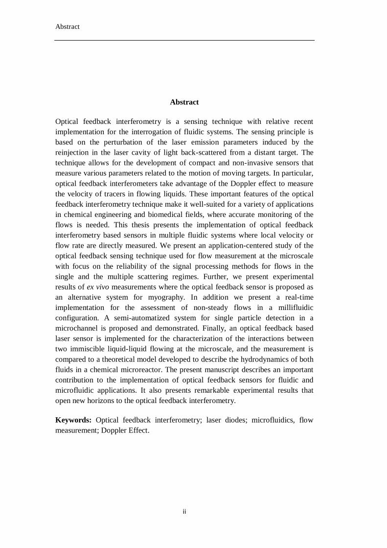
Abstract
Optical feedback interferometry is a sensing technique with relative recent
implementation for the interrogation of fluidic systems. The sensing principle is
based on the perturbation of the laser emission parameters induced by the
reinjection in the laser cavity of light back-scattered from a distant target. The
technique allows for the development of compact and non-invasive sensors that
measure various parameters related to the motion of moving targets. In particular,
optical feedback interferometers take advantage of the Doppler effect to measure
the velocity of tracers in flowing liquids. These important features of the optical
feedback interferometry technique make it well-suited for a variety of applications
in chemical engineering and biomedical fields, where accurate monitoring of the
flows is needed. This thesis presents the implementation of optical feedback
interferometry based sensors in multiple fluidic systems where local velocity or
flow rate are directly measured. We present an application-centered study of the
optical feedback sensing technique used for flow measurement at the microscale
with focus on the reliability of the signal processing methods for flows in the
single and the multiple scattering regimes. Further, we present experimental
results of ex vivo measurements where the optical feedback sensor is proposed as
an alternative system for myography. In addition we present a real-time
implementation for the assessment of non-steady flows in a millifluidic
configuration. A semi-automatized system for single particle detection in a
microchannel is proposed and demonstrated. Finally, an optical feedback based
laser sensor is implemented for the characterization of the interactions between
two immiscible liquid-liquid flowing at the microscale, and the measurement is
compared to a theoretical model developed to describe the hydrodynamics of both
fluids in a chemical microreactor. The present manuscript describes an important
contribution to the implementation of optical feedback sensors for fluidic and
microfluidic applications. It also presents remarkable experimental results that
open new horizons to the optical feedback interferometry.
Keywords: Optical feedback interferometry; laser diodes; microfluidics, flow
measurement; Doppler Effect.
Résumé
iii
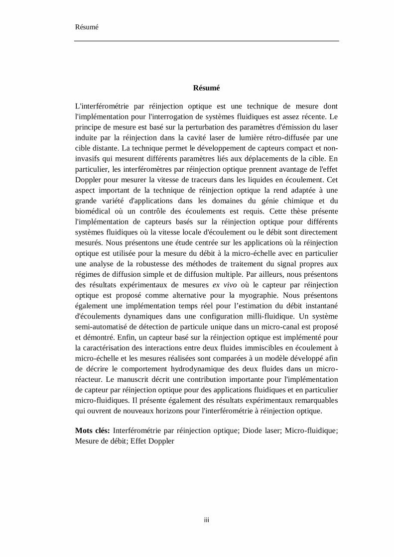
Résumé
L'interférométrie par réinjection optique est une technique de mesure dont
l'implémentation pour l'interrogation de systèmes fluidiques est assez récente. Le
principe de mesure est basé sur la perturbation des paramètres d'émission du laser
induite par la réinjection dans la cavité laser de lumière rétro-diffusée par une
cible distante. La technique permet le développement de capteurs compact et non-
invasifs qui mesurent différents paramètres liés aux déplacements de la cible. En
particulier, les interféromètres par réinjection optique prennent avantage de l'effet
Doppler pour mesurer la vitesse de traceurs dans les liquides en écoulement. Cet
aspect important de la technique de réinjection optique la rend adaptée à une
grande variété d'applications dans les domaines du génie chimique et du
biomédical où un contrôle des écoulements est requis. Cette thèse présente
l'implémentation de capteurs basés sur la réinjection optique pour différents
systèmes fluidiques où la vitesse locale d'écoulement ou le débit sont directement
mesurés. Nous présentons une étude centrée sur les applications où la réinjection
optique est utilisée pour la mesure du débit à la micro-échelle avec en particulier
une analyse de la robustesse des méthodes de traitement du signal propres aux
régimes de diffusion simple et de diffusion multiple. Par ailleurs, nous présentons
des résultats expérimentaux de mesures ex vivo où le capteur par réinjection
optique est proposé comme alternative pour la myographie. Nous présentons
également une implémentation temps réel pour l’estimation du débit instantané
d'écoulements dynamiques dans une configuration milli-fluidique. Un système
semi-automatisé de détection de particule unique dans un micro-canal est proposé
et démontré. Enfin, un capteur basé sur la réinjection optique est implémenté pour
la caractérisation des interactions entre deux fluides immiscibles en écoulement à
micro-échelle et les mesures réalisées sont comparées à un modèle développé afin
de décrire le comportement hydrodynamique des deux fluides dans un micro-
réacteur. Le manuscrit décrit une contribution importante pour l'implémentation
de capteur par réinjection optique pour des applications fluidiques et en particulier
micro-fluidiques. Il présente également des résultats expérimentaux remarquables
qui ouvrent de nouveaux horizons pour l'interférométrie à réinjection optique.
Mots clés: Interférométrie par réinjection optique; Diode laser; Micro-fluidique;
Mesure de débit; Effet Doppler
Acknowledgments
iv
Acknowledgments
I would like to express my deepest gratitude to those who contributed one way or another to the realization of the present thesis.
I thank Prof. Thierry Bosch for giving me the opportunity to join the OSE group at LAAS-CNRS. His continuous disposition and kindness will always be appreciated and remembered.
I have no words to express my gratitude and respects to my supervisor Dr. Julien Perchoux. Your constant guidance and advices pave the way to finally complete this goal. I sincerely say
thanks for your tuition every step of the way. Likewise, I fully thank Prof. Oscar Sotolongo Costa for accepting to supervise my thesis work and for his continuous encouragements and
wise advices through the course of these years. It was indeed an honor to have you both as my
supervisors.
I wanna hereby acknowledge the contributions of my colleagues and friends who collaborated in the development of the present work, particularly those with whom I had the honor to work
with: Lucie Campagnolo, Bendy Tanios, Adam Quotb, Antonio Luna Arriaga, Reza
Atashkhooei, Raül da Costa Moreira and Yu Zhao. I really enjoyed the time we spent together
in and outside the lab! The help provided by Véronique Conédéra and Rémi Courson in the clean room is equally appreciated.
To my dear fellows, I take a chance to reflect here that you will always be remembered as part of the greatest moments in my lifetime. Thank you for all we shared together my friends Jalal
Al Roumy, Laura Le Barbier, Lavinia Ciotirca, Lucas Perbet and Blaise Mulliez, Fernando Urgiles, Harris Apriyanto and Mengkoung Veng. I equally appreciate the time spent with the
stagiaires José Luis, Alejandro, Einar and Fadila as well as the research engineers Valeria,
Allaoua and Gautier.
Likewise, the valuable help and technical assistance provided by Clément Tronche and Francis Jayat is highly appreciated. Thank you both for your disposition. Likewise, I show gratitude for Emmanuelle Tronche and the assistance provided with the intensive paperwork. I also thank the
rest of the members of the OSE group: Francis Bony, Olivier Bernal, Hélène Tap and Han
Cheng Seat.
This thesis is a final step in the research that I conducted in the field of Optical Feedback Interferometry, a technique I learned thank to my former supervisor Prof. Luis Martí López
back in 2009.
The help provided by the Centro de Aplicaciones Tecnológicas y Desarrollo Nuclear in Havana is gratefully appreciated, especially from its former director Dr. Iván Padrón and the members
of the Physics Department who guided me to the conceptualization and realization of the joint co-tuition of the present thesis.
… And the support and continuous encouragements of my family, especially my mother, Marlem, my grandma, my sister and Yancy who were there for me wherever it was necessary.
Thanks!
I acknowledge the financial support provided by the French Embassy in Havana that allowed the funding of the present research work.
v
Contents
Introduction ................................................................................................................ 1
Chapter 1: Doppler systems for flow parameter measurements ............................... 5
1.1 Laser Doppler Velocimetry .................................................................................. 6
1.1.1 History .......................................................................................................... 6
1.1.2 Sensing principle ........................................................................................... 8
1.1.3 Recent developments and commercialization .............................................. 10
1.2 Ultrasound Doppler Velocimetry ....................................................................... 11
1.2.1 History ........................................................................................................ 11
1.2.2 Sensing principle ......................................................................................... 13
1.2.3 Recent developments and commercialization .............................................. 14
1.3 Optical Doppler coherence tomography ............................................................. 15
1.3.1 History ........................................................................................................ 15
1.3.2 Sensing principle ......................................................................................... 16
1.3.4 Recent developments................................................................................... 18
1.4 Planar Doppler velocimetry ............................................................................... 19
1.4.1 History ........................................................................................................ 19
1.4.2 Sensing principle ......................................................................................... 19
1.4.3 Recent developments and commercialization .............................................. 22
1.5 Three Component laser two-focus velocimetry .................................................. 23
1.5.1 Laser two-focus velocimetry ....................................................................... 23
1.5.2 3C-Doppler-L2F Velocimetry .................................................................... 24
1.6 Optical feedback flowmetry ............................................................................... 25
1.6.1 History ........................................................................................................ 25
1.6.2 Sensing principle ......................................................................................... 26
1.6.3 Particular features of optical feedback interferometry .................................. 26
1.7 Comparison of the methods ............................................................................... 27
1.8 Motivations of the present thesis ........................................................................ 29
Chapter 2: Optical feedback interferometry for flows: theoretical fundaments .... 31
2.1 Optical feedback phenomenon for flow measurements ....................................... 32
Contents
vi
2.1.1 Particular features of the interaction laser-fluid ........................................... 32
2.1.2 Theoretical approaches for laser-particles interaction: scattering theories .... 33
2.1.3 The scattering regimes ................................................................................ 36
2.2 Theory of optical feedback applied to multiple scatterers ................................... 39
2.3 Laser characterization under weak feedback ...................................................... 44
2.3.1 Infrared laser characterization ..................................................................... 46
2.3.2 Blue-violet laser characterization ................................................................ 49
Chapter 3: Optical feedback interferometry in fluid flow sensing.......................... 53
3.1 Reliability of optical feedback interferometry .................................................... 54
3.1.1 Processing methods ..................................................................................... 54
3.1.2 Sensor description ....................................................................................... 56
3.1.3 Channel description ..................................................................................... 57
3.1.4 Velocity measurement at channel center ...................................................... 57
3.1.5 Zero order moment for various moving particle concentrations ................... 65
3.1.6 Velocity profile measurement ...................................................................... 67
3.2 Ex-vivo velocity profile measurement ................................................................ 69
3.2.1 OFI pressure myograph sensor .................................................................... 69
3.2.2 Experiment.................................................................................................. 71
3.2.3 Signal processing ........................................................................................ 71
3.2.4 OFI flow mapping ....................................................................................... 72
3.3 Non-steady flow assessment .............................................................................. 74
3.3.1 Signal processing ........................................................................................ 74
3.3.2 Real time implementation............................................................................ 75
3.3.3 Experimental setup ...................................................................................... 76
3.3.4 Unsteady flow interrogation ........................................................................ 77
3.3.5 Non-steady flow velocity measurement ....................................................... 80
3.4 Single particle characterization .......................................................................... 81
3.4.1 Signal detection and processing ................................................................... 82
3.4.2 Particles, flowchannel and experiment......................................................... 83
3.4.3 Theoretical sensing volume ......................................................................... 84
3.4.4 Detected particles ........................................................................................ 84
3.5 Conclusions ....................................................................................................... 86
Chapter 4: Application of optical feedback interferometry to the analysis of
multiphase flows ........................................................................................................ 87
Contents
vii
4.1 General context .................................................................................................. 87
4.2 Theoretical model for parallel liquid-liquid flows .............................................. 90
4.3 Experiments ....................................................................................................... 93
4.3.1 Microfluidic chip ........................................................................................ 93
4.3.2 Fluids .......................................................................................................... 95
4.3.3 Signal processing ........................................................................................ 95
4.3.4 Optoelectronic configurations ..................................................................... 96
4.3.4.1 Single lens configuration ...................................................................... 96
4.3.4.2 Measured profile for single lens configuration ...................................... 97
4.3.4.3 Dual lens configuration ........................................................................ 99
4.3.4.4 Measured profile for dual lens configuration and infrared laser .......... 100
4.3.4.5 Measured profile for dual lens configuration and blue-violet laser ...... 102
4.4 Perspectives ..................................................................................................... 108
Conclusions ............................................................................................................. 109
List of publications .................................................................................................. 113
References ............................................................................................................... 114
Annexes ................................................................................................................... 127

viii
Introduction
- 1 -
Introduction
Optics and photonics are present in everyday’s life, in many technological devices
recently introduced in worldwide markets. In addition, optical and photonic
systems are still generating new discoveries, such as the relatively recent
invention of the blue Light Emitting Diode, which led to three researchers to be
awarded the Nobel Prize in Physics in 2014 as their discovery allowed the
beginning of a new era in lighting applications. Last year was recognized by the
United Nations as the International Year of Light and Light-based Technologies
in a clear effort for emphasizing the top tanked role of optics, lasers and related
disciplines in globalized world under continuous development.
With no doubt, the scientific community has found in optical sciences and
photonic technologies a powerful tool to address cross-disciplinary research
enabling the study, generation and development of new knowledge and
applications in biomedicine, micro-nanotechnology and the environment.
Optical sensing and inspection has gained considerable attention over the last
decades. Optical sensors are attractive for being precise and having non-contact
nature. These elements make optics-based devices suitable for measuring physical
parameters in non-destructive testing, where many other invasive techniques
cannot be used or only with great difficulties. Optical techniques experienced a
significant burst when lasers became available in the scene. The powerful
Introduction
- 2 -
coherent light paved the way to the development of multiple interferometric and
photonics related techniques that are employed today in diverse sensing
applications. In this regard, the optical metrology took benefit from the particular
features of lasers and their contribution to the development of multiple
interferometric techniques that became part of routinely testing protocols in
current manufacturing processes and worldwide production and maintenance.
In addition, the considerable size reduction of components and its combination
with light technologies opens new promising perspectives for advanced imaging
systems that can explore areas that where impossible to access before. This is the
case of the tiny microscope developed recently and represents a major boost in
non-invasive optical imaging of the brain [Kim, 2014].
Optical sensing techniques take benefit from the fact that they use light and non-
destructive interaction with the inspected objects and therefore, they are well-
suited as compared to many other electrical, mechanical, nuclear and chemical
sensors with invasive measurements associated [Baldini, 2006].
Instrumentation and, in particular, optical instrumentation has been extensively
projected as a tool in both laboratory environment and industry for addressing the
measurement of flows. The need for accurate quantitative information of flows is
recognized in the industrial world and laboratory environments.
Fluid flow measurements in microchannels and larger pipes and ducts are
important in multiple processes in industry: chemical engineering, oil production,
water treatment, but also in the biomedical field. To mention a few examples,
microcirculation and blood perfusion in skin is closely related to anomalies in
tissues and may be used as an indicator of potential malignant skin cancers such
as melanomas. Blood flow monitoring in veins and arteries is used for the
assessment of the circulatory system and angiography in human subjects as it may
be used to prevent cardiac arrest. In chemical engineering, there is a vast use of
flows for mixture, solution and transport. The use of flows in multiple
applications in both macro and microscale was followed by the need of providing
accurate velocity measurement in diverse scenarios. In this regard, several
interferometric and image-correlation techniques exist which are widely used for
quantitative and qualitative measurement of flows: speckle patterns, dual-slit,
ultrasonics, particle image velocimetry, laser Doppler velocimetry and others are
well-known and largely implemented techniques in fluid flow assessment.
The merge of optics and microfluidics is known as the cross-disciplinary field of
optofluidics [Psaltis, 2007]. This rather recent denomination obeys to the fact that
many groups dedicated to research on optical measurement technique achieve
outstanding results to understand the behavior of flows at the microscale. Thus,
the terminology optofluidics is nowadays referred to as the field of microfluidic
technology assessed by optical means. Optofluidics has gained considerable
Introduction
- 3 -
attention over the last years and has become a highly active area supported by a
huge number of publications and developments that have revolutionized a wide
range of applications in sensing and imaging [Fainman, 2009].
Although there is a vast amount of detection methods in microfluidics, including
optical, electrical and mass spectrometry methods, the emerging field of
microfluidic sensing has experienced a true fusion with optical measurement
methods, which have become predominant in the field since its earliest
developments [Wu, 2011]. Optical sensing comprise the direct detection of the
flow in microfluidic devices by monitoring the light properties modulation due to
the interaction light-flow.
Throughout this thesis, we propose to deploy optical feedback interferometry
sensors for multiple sensing applications in fluidic systems, with strong emphasis
in microfluidics. The experimental demonstrations presented in the frame of this
manuscript accentuate the potential of this technique as an alternative optofluidic
implementation system. We thereby utilize the capabilities of this technique for
the interrogation of fluid flows with focus on the applicability in the chemical and
biomedical field.
Several demonstrations of the potential applications of optical feedback effect and
its use in optical sensing are provided and discussed in the present manuscript.
The document is organized as follows:
Chapter 1 presents a review of the Doppler methods used for the analysis of
flows. The main fundaments of the Doppler Effect are presented and the
techniques using it explained in the frame of historical aspects, sensing system,
recent developments associated and commercialization. We identified several
largely used techniques and outline the relative aspects for every technique. The
chapter presents Laser Doppler velocimetry, ultrasound Doppler velocimetry,
optical Doppler coherence tomography, planar Doppler velocimetry, three-
components laser two-focus velocimetry and finally optical feedback flowmetry.
In the end of the chapter, a comparison of the techniques is provided as well as the
main motivations of the present thesis manuscript are exposed.
The second chapter presents the sensing mechanism on which optical feedback
interferometry is based. The chapter presents first the basics of the scattering
theories and then the fundaments of the optical feedback effect. In the final part of
the chapter, a section is dedicated to a detailed description of the characterization
of the lasers used in this thesis.
Chapter 3 presents a huge portion of the experimental results obtained during the
development of the present thesis. We describe the main processing methods used
to quantify the flow velocity with optical feedback interferometry and present a
complete analysis of the reliability of the flow measurement with this technique.
The chapter continues with a demonstration of an ex-vivo flow mapping. Then, a
Introduction
- 4 -
real-time system allowing the assessment of non-steady flows is presented and
validated experimentally. The final section of the chapter presents a portion of an
ongoing research work on single particle detection in microfluidic devices, which
is proposed as a quality control system consisting on the inspection of fluids that
should be free of particles.
The final chapter presents the implementation of the optical feedback
interferometry sensing technique for the analysis of immiscible multiphase flows.
A theoretical model based developed from the Couette flow approximation is
proposed. The model is further validated with experimental measurements fluid
velocity profile in microfluidic reactors.
In the end, a general conclusion is given and further perspectives are proposed.
Chapter 1: Doppler methods for flow measurements
- 5 -
Chapter 1
Doppler methods for flow measurements
In this chapter, some of the well-established techniques based on the Doppler
Effect for flow measurements are reviewed and compared. In what follows, Laser
Doppler Velocimetry, Ultrasonic Doppler Velocimetry, Optical Doppler
Coherence Tomography, Planar Doppler Velocimetry, Three component laser-
two-focus velocimetry and finally, Optical Feedback Flowmetry are reviewed to
provide a general understanding of the historical and technological aspects that
were developed to be part of the widely spread techniques allowing fluid flow
assessment using the Doppler Effect.
The Doppler Effect
The Doppler Effect is defined as a change in the frequency of a wave when the
reference observer moves towards or away from the source. It was named after
Chapter 1: Doppler methods for flow measurements
- 6 -
Christian Doppler, an Austrian scientist who proposed the first explanation of the
phenomenon in 1842 in the frame of a meeting of the Natural Sciences Section of
the Royal Bohemian Society of Sciences in Prague. Doppler’s paper entitled “On
the colored light of the double stars and certain other stars in heavens” was
published in 1843 in the proceedings of the society [Doppler, 1843].
To provide a simple approach to the physics behind the Doppler Effect, let’s
consider a stationary light source emitting with a given wavelength λ and
frequency 𝑓. The wave train with length λ needs a time 𝑇 = 1 𝑓⁄ to pass a
stationary observer. If the observer moves away from the light source the distance
between them increases, and the waves would need more time (𝑇′ > 𝑇) to reach
the observer. As the distance is modified, an equation describing this parameter
can be set. The total distance 𝑐𝑇′ separating the observer and the source will be
composed of the length λ plus the distance moved 𝑣𝑇′, where 𝑐 is the speed of
light and 𝑣 is the velocity of the observer. The equation giving the distance is:
𝑐𝑇′ = 𝜆 + 𝑣𝑇′ (1.1)
which leads to
𝜆 = (𝑐 − 𝑣)𝑇′ (1.2)
Knowing that the new period is the inverse of the wave’s frequency resulting from
the displacement of the observer 𝑇′ = 1 𝑓′⁄ , 𝜆 = 𝑐 𝑓⁄ and substituting into
equation 1.2, the relation between the orginal frequency and the one perceived by
the observer is:
𝑓′ = [1 −𝑣
𝑐] 𝑓 (1.3)
From expression 1.3 follows that if the observer moves away from the source
(𝑣 > 0) the new frequency is shifted to smaller values. If, on the contrary, the
observer moves towards the source, the frequency shift increases.
1.1 Laser Doppler Velocimetry
The Laser Doppler Velocimetry (LDV) also referred to as Laser Doppler
Anemometry was the first mature technique for flow measurement to be available
for implementation. Since the sixties, soon after the laser appeared as a solution
looking for problems, the LDV has been used in numerous applications ranging
from aeronautics and turbomachinery to ophthalmology and other biomedical
fields [Menn, 2004]. The main purpose of the technique lies in measuring the
velocity and/or the length of moving surfaces.
1.1.1 History
Back in 1964, two scientists working on Rayleigh scattering modified a
spectrometer with the idea of using the Doppler Effect to measure the velocity of
particles flowing in a liquid. At that time, LDV was introduced by Yeh and
Chapter 1: Doppler methods for flow measurements
- 7 -
Cummins [1964]. In this work, the coherent light source was a He-Ne gas laser.
Using optical elements, they split a laser beam and used one beam as a reference
while the other was directed to illuminate a volume full of polystyrene spheres in
water. After this interaction with the particles, the two beams were combined in a
photomultiplier and the frequency shift was retrieved by processing the beat
signal.
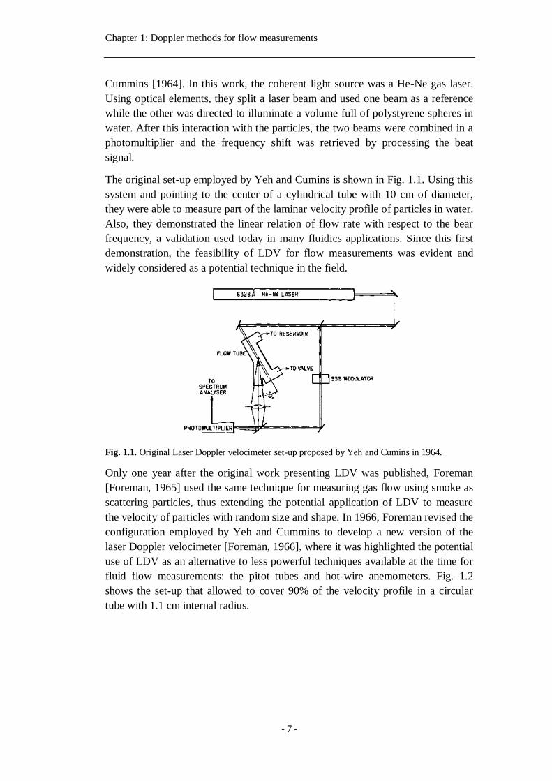
The original set-up employed by Yeh and Cumins is shown in Fig. 1.1. Using this
system and pointing to the center of a cylindrical tube with 10 cm of diameter,
they were able to measure part of the laminar velocity profile of particles in water.
Also, they demonstrated the linear relation of flow rate with respect to the bear
frequency, a validation used today in many fluidics applications. Since this first
demonstration, the feasibility of LDV for flow measurements was evident and
widely considered as a potential technique in the field.
Fig. 1.1. Original Laser Doppler velocimeter set-up proposed by Yeh and Cumins in 1964.
Only one year after the original work presenting LDV was published, Foreman
[Foreman, 1965] used the same technique for measuring gas flow using smoke as
scattering particles, thus extending the potential application of LDV to measure
the velocity of particles with random size and shape. In 1966, Foreman revised the
configuration employed by Yeh and Cummins to develop a new version of the
laser Doppler velocimeter [Foreman, 1966], where it was highlighted the potential
use of LDV as an alternative to less powerful techniques available at the time for
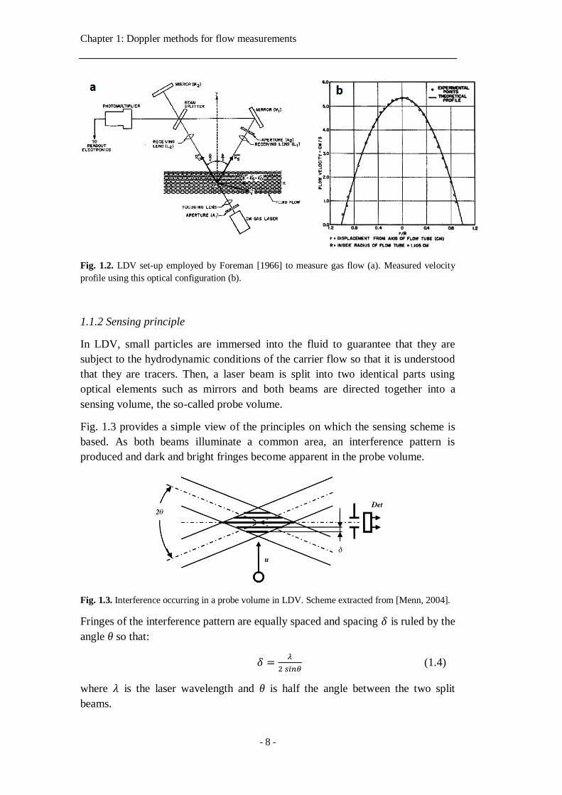
fluid flow measurements: the pitot tubes and hot-wire anemometers. Fig. 1.2
shows the set-up that allowed to cover 90% of the velocity profile in a circular
tube with 1.1 cm internal radius.
Chapter 1: Doppler methods for flow measurements
- 8 -
Fig. 1.2. LDV set-up employed by Foreman [1966] to measure gas flow (a). Measured velocity
profile using this optical configuration (b).
1.1.2 Sensing principle
In LDV, small particles are immersed into the fluid to guarantee that they are
subject to the hydrodynamic conditions of the carrier flow so that it is understood
that they are tracers. Then, a laser beam is split into two identical parts using
optical elements such as mirrors and both beams are directed together into a
sensing volume, the so-called probe volume.
Fig. 1.3 provides a simple view of the principles on which the sensing scheme is
based. As both beams illuminate a common area, an interference pattern is
produced and dark and bright fringes become apparent in the probe volume.
Fig. 1.3. Interference occurring in a probe volume in LDV. Scheme extracted from [Menn, 2004].
Fringes of the interference pattern are equally spaced and spacing 𝛿 is ruled by the
angle θ so that:
𝛿 =𝜆
2 𝑠𝑖𝑛𝜃 (1.4)
where 𝜆 is the laser wavelength and θ is half the angle between the two split
beams.
Chapter 1: Doppler methods for flow measurements
- 9 -
When a particle moves through the probe volume with velocity 𝑣𝑝, it crosses dark
and bright fringes so that the intensity of the scattered light varies with a
frequency 𝑓𝑝:
𝑓𝑝 =𝑣𝑝
𝛿 (1.5)
Photodetected signals contain information on the frequency, and the velocity of
the particles in the probe volume is determined by:
𝑣𝑝 =𝜆
2 𝑠𝑖𝑛𝜃𝑓𝑝 (1.6)
This detection system was first proposed by Rudd back in 1969 [Rudd, 1969].
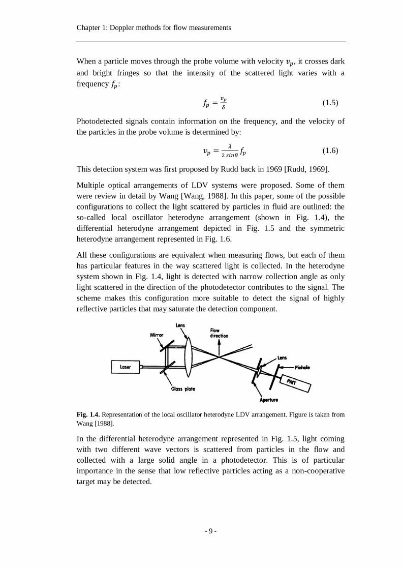
Multiple optical arrangements of LDV systems were proposed. Some of them
were review in detail by Wang [Wang, 1988]. In this paper, some of the possible
configurations to collect the light scattered by particles in fluid are outlined: the
so-called local oscillator heterodyne arrangement (shown in Fig. 1.4), the
differential heterodyne arrangement depicted in Fig. 1.5 and the symmetric
heterodyne arrangement represented in Fig. 1.6.
All these configurations are equivalent when measuring flows, but each of them
has particular features in the way scattered light is collected. In the heterodyne
system shown in Fig. 1.4, light is detected with narrow collection angle as only
light scattered in the direction of the photodetector contributes to the signal. The
scheme makes this configuration more suitable to detect the signal of highly
reflective particles that may saturate the detection component.
Fig. 1.4. Representation of the local oscillator heterodyne LDV arrangement. Figure is taken from
Wang [1988].
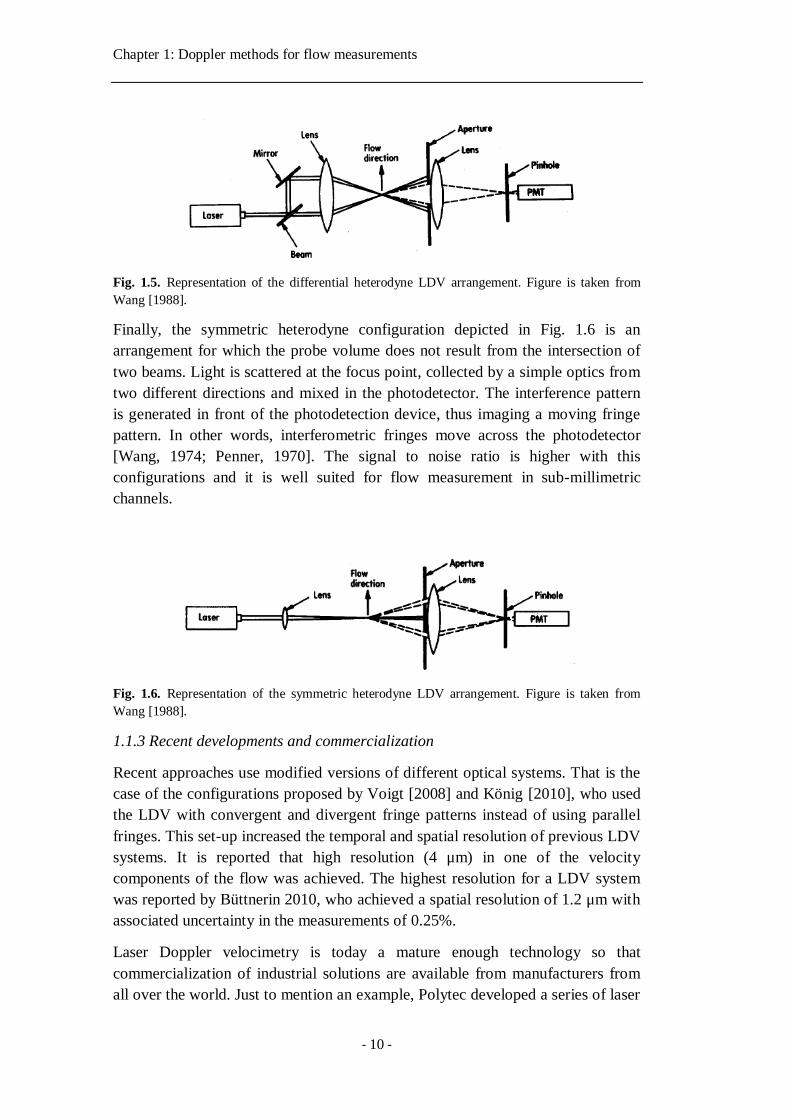
In the differential heterodyne arrangement represented in Fig. 1.5, light coming
with two different wave vectors is scattered from particles in the flow and
collected with a large solid angle in a photodetector. This is of particular
importance in the sense that low reflective particles acting as a non-cooperative
target may be detected.
Chapter 1: Doppler methods for flow measurements
- 10 -
Fig. 1.5. Representation of the differential heterodyne LDV arrangement. Figure is taken from
Wang [1988].
Finally, the symmetric heterodyne configuration depicted in Fig. 1.6 is an
arrangement for which the probe volume does not result from the intersection of
two beams. Light is scattered at the focus point, collected by a simple optics from
two different directions and mixed in the photodetector. The interference pattern
is generated in front of the photodetection device, thus imaging a moving fringe
pattern. In other words, interferometric fringes move across the photodetector
[Wang, 1974; Penner, 1970]. The signal to noise ratio is higher with this
configurations and it is well suited for flow measurement in sub-millimetric
channels.
Fig. 1.6. Representation of the symmetric heterodyne LDV arrangement. Figure is taken from
Wang [1988].
1.1.3 Recent developments and commercialization
Recent approaches use modified versions of different optical systems. That is the
case of the configurations proposed by Voigt [2008] and König [2010], who used
the LDV with convergent and divergent fringe patterns instead of using parallel
fringes. This set-up increased the temporal and spatial resolution of previous LDV
systems. It is reported that high resolution (4 μm) in one of the velocity
components of the flow was achieved. The highest resolution for a LDV system
was reported by Büttnerin 2010, who achieved a spatial resolution of 1.2 μm with
associated uncertainty in the measurements of 0.25%.
Laser Doppler velocimetry is today a mature enough technology so that
commercialization of industrial solutions are available from manufacturers from
all over the world. Just to mention an example, Polytec developed a series of laser
Chapter 1: Doppler methods for flow measurements
- 11 -
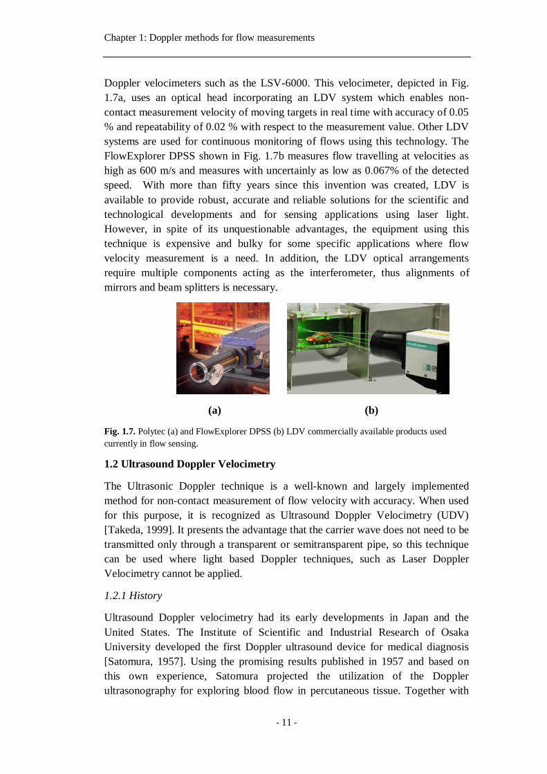
Doppler velocimeters such as the LSV-6000. This velocimeter, depicted in Fig.
1.7a, uses an optical head incorporating an LDV system which enables non-
contact measurement velocity of moving targets in real time with accuracy of 0.05
% and repeatability of 0.02 % with respect to the measurement value. Other LDV
systems are used for continuous monitoring of flows using this technology. The
FlowExplorer DPSS shown in Fig. 1.7b measures flow travelling at velocities as
high as 600 m/s and measures with uncertainly as low as 0.067% of the detected
speed. With more than fifty years since this invention was created, LDV is
available to provide robust, accurate and reliable solutions for the scientific and
technological developments and for sensing applications using laser light.
However, in spite of its unquestionable advantages, the equipment using this
technique is expensive and bulky for some specific applications where flow
velocity measurement is a need. In addition, the LDV optical arrangements
require multiple components acting as the interferometer, thus alignments of
mirrors and beam splitters is necessary.
(a) (b)
Fig. 1.7. Polytec (a) and FlowExplorer DPSS (b) LDV commercially available products used
currently in flow sensing.
1.2 Ultrasound Doppler Velocimetry
The Ultrasonic Doppler technique is a well-known and largely implemented
method for non-contact measurement of flow velocity with accuracy. When used
for this purpose, it is recognized as Ultrasound Doppler Velocimetry (UDV)
[Takeda, 1999]. It presents the advantage that the carrier wave does not need to be
transmitted only through a transparent or semitransparent pipe, so this technique
can be used where light based Doppler techniques, such as Laser Doppler
Velocimetry cannot be applied.
1.2.1 History
Ultrasound Doppler velocimetry had its early developments in Japan and the
United States. The Institute of Scientific and Industrial Research of Osaka
University developed the first Doppler ultrasound device for medical diagnosis
[Satomura, 1957]. Using the promising results published in 1957 and based on
this own experience, Satomura projected the utilization of the Doppler
ultrasonography for exploring blood flow in percutaneous tissue. Together with
Chapter 1: Doppler methods for flow measurements
- 12 -
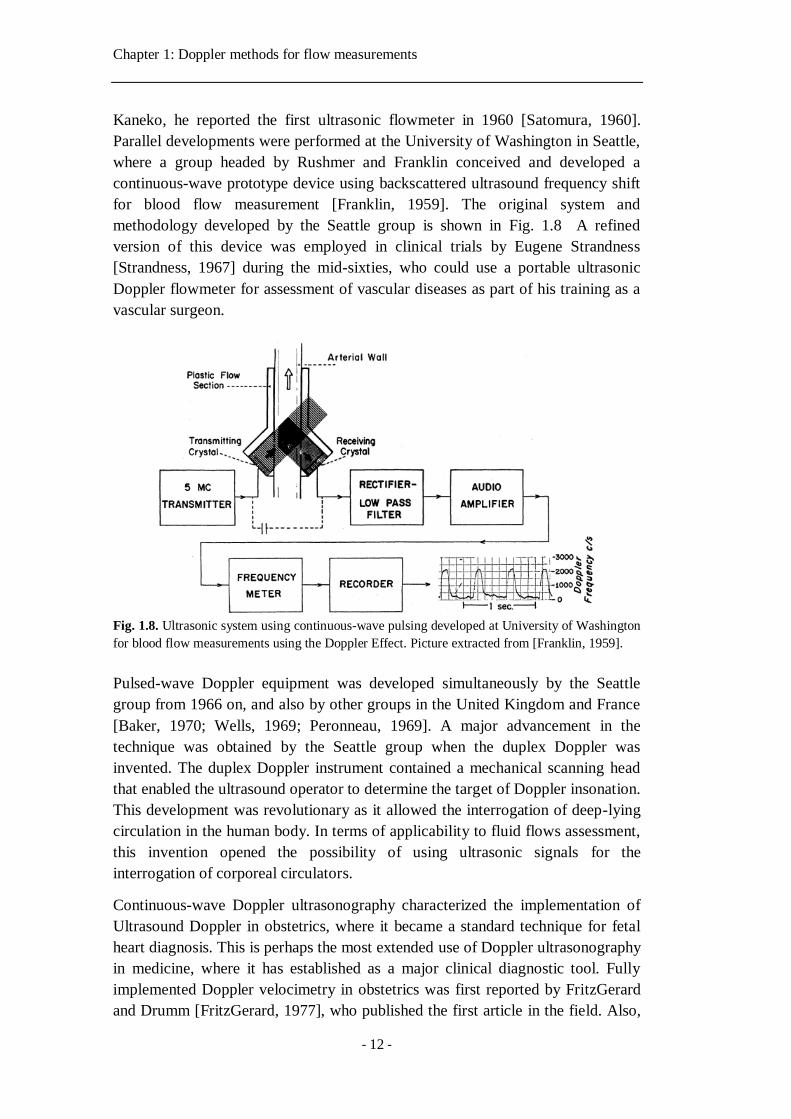
Kaneko, he reported the first ultrasonic flowmeter in 1960 [Satomura, 1960].
Parallel developments were performed at the University of Washington in Seattle,
where a group headed by Rushmer and Franklin conceived and developed a
continuous-wave prototype device using backscattered ultrasound frequency shift
for blood flow measurement [Franklin, 1959]. The original system and
methodology developed by the Seattle group is shown in Fig. 1.8 A refined
version of this device was employed in clinical trials by Eugene Strandness
[Strandness, 1967] during the mid-sixties, who could use a portable ultrasonic
Doppler flowmeter for assessment of vascular diseases as part of his training as a
vascular surgeon.
Fig. 1.8. Ultrasonic system using continuous-wave pulsing developed at University of Washington
for blood flow measurements using the Doppler Effect. Picture extracted from [Franklin, 1959].
Pulsed-wave Doppler equipment was developed simultaneously by the Seattle
group from 1966 on, and also by other groups in the United Kingdom and France
[Baker, 1970; Wells, 1969; Peronneau, 1969]. A major advancement in the
technique was obtained by the Seattle group when the duplex Doppler was
invented. The duplex Doppler instrument contained a mechanical scanning head
that enabled the ultrasound operator to determine the target of Doppler insonation.
This development was revolutionary as it allowed the interrogation of deep-lying
circulation in the human body. In terms of applicability to fluid flows assessment,
this invention opened the possibility of using ultrasonic signals for the
interrogation of corporeal circulators.
Continuous-wave Doppler ultrasonography characterized the implementation of
Ultrasound Doppler in obstetrics, where it became a standard technique for fetal
heart diagnosis. This is perhaps the most extended use of Doppler ultrasonography
in medicine, where it has established as a major clinical diagnostic tool. Fully
implemented Doppler velocimetry in obstetrics was first reported by FritzGerard
and Drumm [FritzGerard, 1977], who published the first article in the field. Also,
Chapter 1: Doppler methods for flow measurements
- 13 -
McCallum and colleagues, who at the time were part of the Seattle group at
University of Washington, pioneered the real time implementation of this
technique [McCallum, 1977].
1.2.2 Sensing principle
Ultrasonic Doppler flowmeters operate using the frequency shift that a sound
wave experiences due to the Doppler Effect. Usually, a transducer is employed to
transmit a wave through a medium, and the moving components in the medium
generate a shift in the carrier signal. The motion is measured after comparing
frequency shift between the ultrasonic frequency source, the receiver and the fluid
carrier.
The sound wave emitted by the transducer in the ultrasonic Doppler device travels
from the face of the sensor to the flow stream. When the wave intercepts a moving
particle merged in the flow, its frequency is shifted and consequently it differs
from the original source frequency. Due to the Doppler Effect, if particles move
toward the transducer, the Doppler-shifted wave will contain higher frequencies
than the transmitted wave. In terms of mathematical representation, this process is
described by the Doppler equation:
𝑣 =𝑣𝑚(𝑓𝑟−𝑓𝑡)
2𝑓𝑡𝑐𝑜𝑠(𝜑) (1.7)
where 𝑣𝑚 is the velocity of the sound wave in the medium is, 𝑓𝑡 is the transmitted
wave frequency, 𝑓𝑟 is the received wave frequency and 𝜑 is the angle between the
transmitted ultrasound beam and the flow velocity vector. Equation 1.7 implicates
that the angle 𝜑 should be precisely determined to obtain an accurate
measurement of velocity.
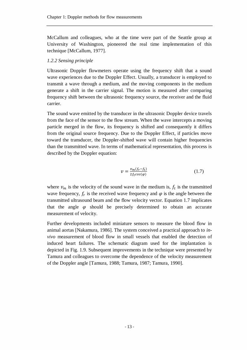
Further developments included miniature sensors to measure the blood flow in
animal aortas [Nakamura, 1986]. The system conceived a practical approach to in-
vivo measurement of blood flow in small vessels that enabled the detection of
induced heart failures. The schematic diagram used for the implantation is
depicted in Fig. 1.9. Subsequent improvements in the technique were presented by
Tamura and colleagues to overcome the dependence of the velocity measurement
of the Doppler angle [Tamura, 1988; Tamura, 1987; Tamura, 1990].
Chapter 1: Doppler methods for flow measurements
- 14 -
Fig. 1.9. Implanted Ultrasonic Doppler Flowmeter proposed by Nakamura et al. for in-vivo
measurement of blood flow.
In 1986, Takeda presented an ultrasonic blood flowmeter capable of measuring
the entire flow profile of millimetric channels with a spatial resolution of 0.7 mm.
Akamatsu developed an Ultrasound Doppler catheter insensitive to the angle of
incidence of the source wave [Akamatsu, 1996]. Instead of using the classical
expression represented in Eq. 1.6, they proposed a methodology considering a
measurement at two different angles (α and α+Ω) thus obtaining a new expression
for calculation of the flow velocity: 𝑣 = (𝑣12 + 𝑣2
2)1/2 which becomes:
𝑣 =𝑣𝑚
2𝑓𝑡(∆𝑓1
2 + ∆𝑓22)1/2 (1.8)
While the theoretical fundaments were correct, the method has not been
implemented, the main obstacle being that two separated beams need to be
emitted to a common point with different Doppler angles.
1.2.3 Recent developments and commercialization
Other challenges related to UDV for flow assessment include the capability of
measuring flow velocities higher than the maximum detectable velocity imposed
in the Nyquist theorem. As the physical principle of supporting this technology
depends on the velocity of propagation of the carrier ultrasonic wave, aliasing
may arise as fast flows are measured.
Murakawa recently addressed this technical limitation. They proposed a method
with dual-pulsed repetition frequency for ultrasonic flow measurements
[Murakawa, 2015]. The method is aimed at overcoming the aliasing in the
velocity detection, thus providing a way to extend the applicability of UDV to
sense flow travelling at high velocities. In addition, the spatial resolution of the
UDV sensing system achieved with this configuration ranges in between 0.74 and
2.96 mm.
Utrasound Doppler Flowmeters are accurate, non-contact liquid flow measuring
devices. These devices are commercially available to satisfy the demands of the
industry, where flows can be measured non-destructively even in adverse
scenarios.
Chapter 1: Doppler methods for flow measurements
- 15 -
Research on UDV made possible that knowledge generated around the technique
facilitated its implementation in commercial products available since many years.
One can mention, for example, the Hitachi EUD-3B professional ultrasonic
velocimeter capable to measuring flows [Nakamura, 1986]. Other technological
UDV solutions are found in large water storage facilities, as for example the ISCO
4150 Doppler velocimeter which continuously measures the flow stream profile
and automatically detects changes in the velocity distribution. Today, the
technique is supported by a vast state of the art that enabled the extended use of
UDV in laboratories, industry and as a valuable tool in in-field flow assessment.
1.3 Optical Doppler Coherence Tomography
Doppler Optical Coherence Tomography is a relatively recent technique using
low-coherent light combined with the Doppler Effect to visualize and quantify
mostly blood flow. Since early nineties, many studies have been performed to
extract information on pathological structures and angiographic components in
living subjects, where the utilization of this technique has provided the specialists
with valuable data allowing diagnosis and assessment of morphology of tissue and
microcirculation without any invasiveness. Thereby, implementation of this
technique in medical studies opened promising perspectives in ophthalmology and
angiography [Leitgeb, 2014] as well as in gastroenterology [Osiac, 2011].
1.3.1 History
The history of Optical Coherence Tomography (OCT) dates back to the early
nineties, when it found its bases upon the development of low coherence
interferometry. A group headed by professor Fujimoto from the Massachusetts
Institute of Technology pioneered the first developments in the technique [Huang,
1991; Swanson, 1993]. OCT shares some similarities with ultrasound and both
techniques are usually compared in experimental work reported in the literature.
However, OCT is capable of providing high resolution cross sectional images
allowing 3D mapping of samples. In early nineties, there was little availability for
alternative imaging systems working at higher resolutions than the one allowed by
high-frequency ultrasound and greater penetration depth than that of confocal
microscopy [Drexel, 2004; Rajadhyaksha, 1999]. First applications included the
study of tissue structure and targeted OCT’s direct implementation in diverse
medical domains, predominantly in ophthalmology.
Doppler OCT, also referred to as Optical Doppler Tomography (ODT) combines
the fundamental principles of low coherence tomography and the Doppler Effect.
It is an extension of classical OCT, aiming at outlining the morphology of tissue
and providing values for the underlying microcirculation in this tissue. Moreover,
ODT possesses a unique capability to be implemented for qualitative investigation
of tissue shape and localization of vessels and arteries within living structures and
Chapter 1: Doppler methods for flow measurements
- 16 -
at the same time, it allows quantitative study of blood velocity associated with the
circulatory system.
It should be noted, that most of research on OCT lies at the intersection of
biomedical research and clinical diagnosis. As compared to other methods, OCT
uses light in the visible and infrared region, so photons are less energetic than
photons used in X-ray and gamma-ray systems widely used in medical imaging
which have the inconvenient that they could damage biological samples [Boppart,
2004; Sun, 2013]. This makes OCT based diagnosis more suitable in clinical
inspection and cancer diagnosis.
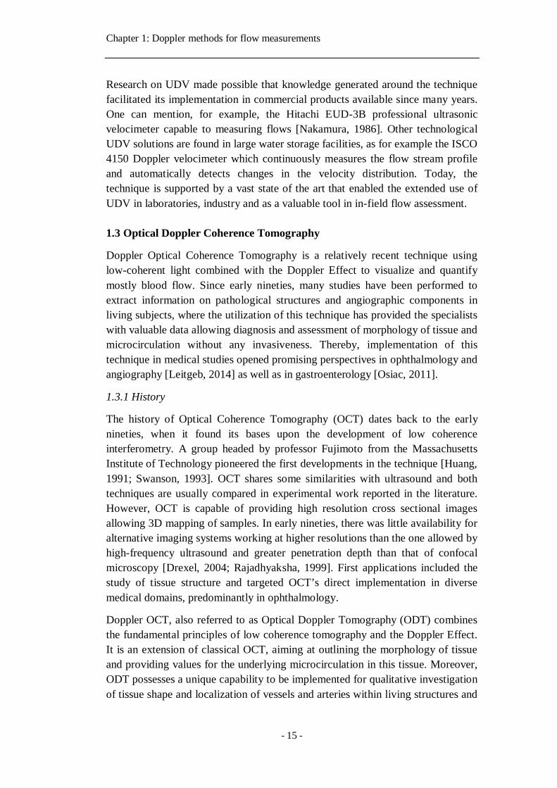
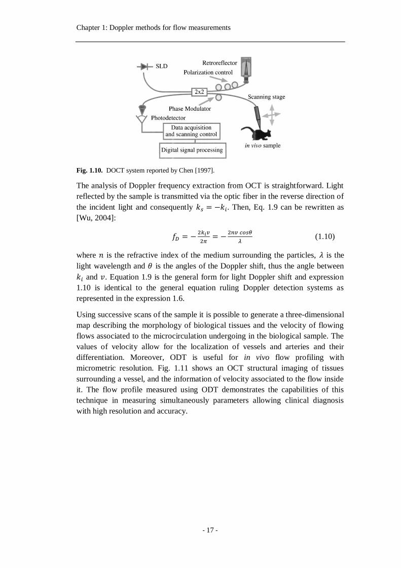
1.3.2 Sensing principle
ODT is non-invasive in nature as it uses low coherent light for inspection of the
sample. The first set-up reported used a fiber Michelson interferometer associated
to an automated translation stage for producing a three-dimensional image of
tissue microstructures. This set-up is depicted in Fig. 1.10. Light emitted form a
superluminescent diode (SLD) is partially directed into a reference arm in the
interferometer and the other part is headed to the sample arm. The reference arm
contains a mirror coupled to a longitudinal displacement mechanism and the
sample arm allows displacement in the sense of the desired scan direction of the
sample.
The sensing purpose of this technique lies in scanning the reference mirror arm
and recording the amplitude of the interference pattern generated by the waves
with similar path length. As stated above, ODT uses a combination of OCT with
the information extracted from the Doppler Effect. Its first application in 2D
imaging dates back to 1997, when the technique extended the use of OCT for
obtaining quantitative values of blood flow velocity [Chen, 1997]. Light
backscattered from moving elements (or particles) interferes with the light taken
as a reference and its frequency is Doppler shifted in the interference pattern
intensity. This shift is characterized by an amount given by [Chen, 1997]:
𝑓𝐷 =1
2𝜋(𝒌𝒔 − 𝒌𝒊)𝒗 (1.9)
where 𝑘𝑖 and 𝑘𝑠 are wave vectors of incoming and scattered light respectively,
and 𝑣 is the velocity of moving particles.
Chapter 1: Doppler methods for flow measurements
- 17 -
Fig. 1.10. DOCT system reported by Chen [1997].
The analysis of Doppler frequency extraction from OCT is straightforward. Light
reflected by the sample is transmitted via the optic fiber in the reverse direction of
the incident light and consequently 𝑘𝑠 = −𝑘𝑖. Then, Eq. 1.9 can be rewritten as
[Wu, 2004]:
𝑓𝐷 = −2𝑘𝑖𝑣
2𝜋= −
2𝑛𝑣 𝑐𝑜𝑠𝜃
𝜆 (1.10)
where 𝑛 is the refractive index of the medium surrounding the particles, 𝜆 is the
light wavelength and 𝜃 is the angles of the Doppler shift, thus the angle between
𝑘𝑖 and 𝑣. Equation 1.9 is the general form for light Doppler shift and expression
1.10 is identical to the general equation ruling Doppler detection systems as
represented in the expression 1.6.
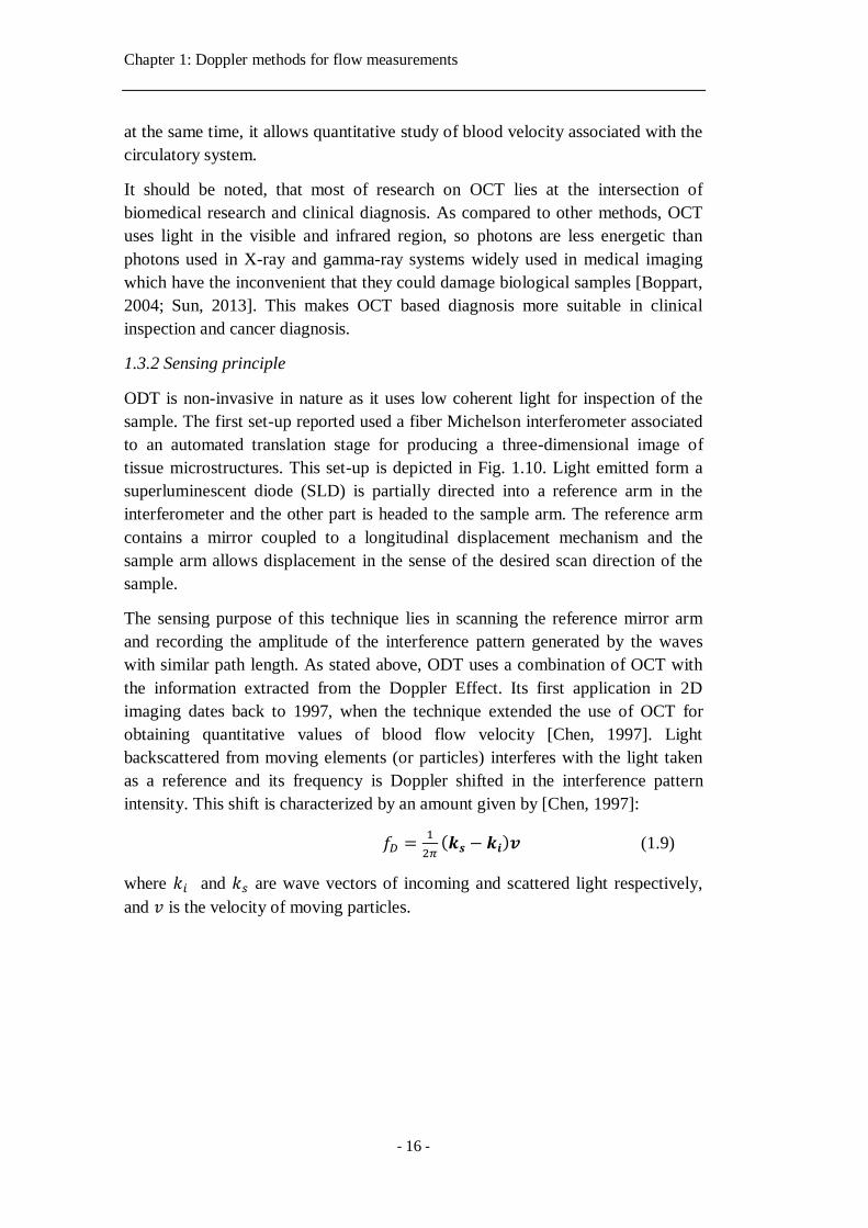
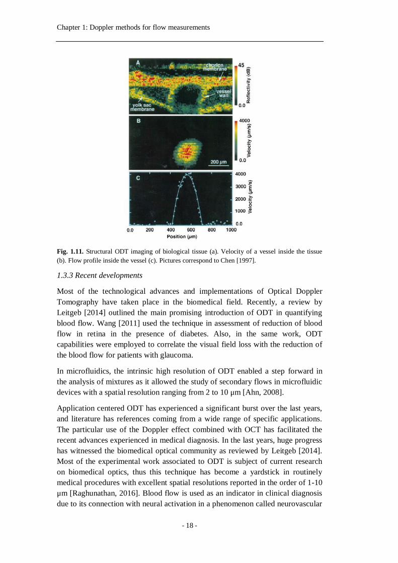
Using successive scans of the sample it is possible to generate a three-dimensional
map describing the morphology of biological tissues and the velocity of flowing
flows associated to the microcirculation undergoing in the biological sample. The
values of velocity allow for the localization of vessels and arteries and their
differentiation. Moreover, ODT is useful for in vivo flow profiling with
micrometric resolution. Fig. 1.11 shows an OCT structural imaging of tissues
surrounding a vessel, and the information of velocity associated to the flow inside
it. The flow profile measured using ODT demonstrates the capabilities of this
technique in measuring simultaneously parameters allowing clinical diagnosis
with high resolution and accuracy.
Chapter 1: Doppler methods for flow measurements
- 18 -
Fig. 1.11. Structural ODT imaging of biological tissue (a). Velocity of a vessel inside the tissue
(b). Flow profile inside the vessel (c). Pictures correspond to Chen [1997].
1.3.3 Recent developments
Most of the technological advances and implementations of Optical Doppler
Tomography have taken place in the biomedical field. Recently, a review by
Leitgeb [2014] outlined the main promising introduction of ODT in quantifying
blood flow. Wang [2011] used the technique in assessment of reduction of blood
flow in retina in the presence of diabetes. Also, in the same work, ODT
capabilities were employed to correlate the visual field loss with the reduction of
the blood flow for patients with glaucoma.
In microfluidics, the intrinsic high resolution of ODT enabled a step forward in
the analysis of mixtures as it allowed the study of secondary flows in microfluidic
devices with a spatial resolution ranging from 2 to 10 μm [Ahn, 2008].
Application centered ODT has experienced a significant burst over the last years,
and literature has references coming from a wide range of specific applications.
The particular use of the Doppler effect combined with OCT has facilitated the
recent advances experienced in medical diagnosis. In the last years, huge progress
has witnessed the biomedical optical community as reviewed by Leitgeb [2014].
Most of the experimental work associated to ODT is subject of current research
on biomedical optics, thus this technique has become a yardstick in routinely
medical procedures with excellent spatial resolutions reported in the order of 1-10
μm [Raghunathan, 2016]. Blood flow is used as an indicator in clinical diagnosis
due to its connection with neural activation in a phenomenon called neurovascular
Chapter 1: Doppler methods for flow measurements
- 19 -
coupling [Attwell, 2010]. Also, this technique provided sensitive quantitative data
for the study of retinopathy and the influence of diabetes in it [Wang, 2009].
1.4 Planar Doppler velocimetry
The experience generated with the advent of the laser and its use in flow
measurements pioneered by Yeh and Cummins [Yeh, 1964] pave the way to
further developments integrating the Doppler Effect with optics and laser
technology and its potential utilization in measuring flow velocity. Planar Doppler
Velocimetry (PDV), also known as Doppler Global Velocimetry is another optical
technique with relative recent presence in the analysis of flows. This technique
uses a planar imaging configuration of the light emitted by a laser that illuminates
a medium with particles. The scattering produced by these particles is used for the
measurement of a Doppler frequency shift of backscattered light to further turn it
into an intensity distribution.
1.4.1 History
In 1991, Komine and Brosnan developed the original Global Doppler Velocimeter
using a molecular filter to identify the Doppler shift in scattered light generated by
particles in a flow illuminated with a laser [Komine, 1991]. The idea is based on
the concept of the filtered scattering produced by small particles and molecules in
the flow [Miles, 1990]. The technique was rapidly introduced in the analysis of
mixing [Elliot, 1992] and flows travelling at high velocities [Elliot, 1994].
McKenzie explored PDV in flow assessment using a pulsed laser [McKenzie,
1996] and presented the capabilities of the technique in measuring slow flows
[McKenzie, 1997]. Several groups accelerated the implementation of PDV to
visualize fast processes in fluid, including velocity measurements of supersonic
jets [Clancy, 1997; Clancy, 1999]. During the development and consolidation of
the technique, authors started to denominate it as Planar Doppler Velocimetry,
that was found to be more precise than Doppler Global Velocimetry, but any of
these terms is found in the current literature.
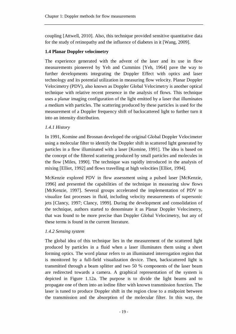
1.4.2 Sensing system
The global idea of this technique lies in the measurement of the scattered light
produced by particles in a fluid when a laser illuminates them using a sheet
forming optics. The word planar refers to an illuminated interrogation region that
is monitored by a full-field visualization device. Then, backscattered light is
transmitted through a beam splitter and two 50 % components of the laser beam
are redirected towards a camera. A graphical representation of the system is
depicted in Figure 1.12a. The purpose is to divide the light beams and to
propagate one of them into an iodine filter with known transmission function. The
laser is tuned to produce Doppler shift in the region close to a midpoint between
the transmission and the absorption of the molecular filter. In this way, the
Chapter 1: Doppler methods for flow measurements
- 20 -
variations of the intensity of light are proportional to the Doppler shift produced
by the scattering centers of the flow. Both intensity images obtained with the
cameras are compared and by normalizing the intensity values the variations of
the flow velocity can be quantified.
(a) (b)
Fig. 1.12. PDV system for flow measurements using a reference camera and a signal (filtered)
camera (a). Measured qualitative velocity (b).
In its simplest configuration, this set-up can be used for quantifying complex
flows fields using the rate capabilities of a visualization device such as cameras
[Meyers, 1992]. Since the early introduction of this technique, it has been
considered as a step forward towards full-field flow measurements beyond single
point measuring scheme. Is this particularly useful in the qualitative visualization
of vortex trajectories and other features of complex flow that are difficult to
measure [Samimy, 2000; Elliott, 1999]. The Doppler shift of scattered light is
then measured using the expression 1.6.
Chapter 1: Doppler methods for flow measurements
- 21 -
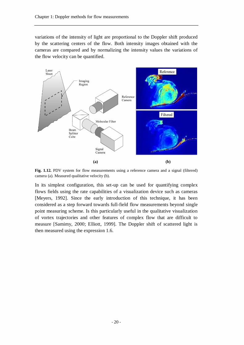
Fig. 1.13. PVD systems based on a single visualization system. Image belongs to reference
[Samimy, 2000].
However, it should be pointed out, that measuring the Doppler shift is necessary
in the implementation of the technique but not fully sufficient for measuring the
desired velocity of the flow. The set-up described in Figure 1.13 is sensitive to
obtain velocities components in the direction s u . In order to measure all
possible components of flow velocity the detection system needs to be modified
so that the scattering produced by particles is observed from three different
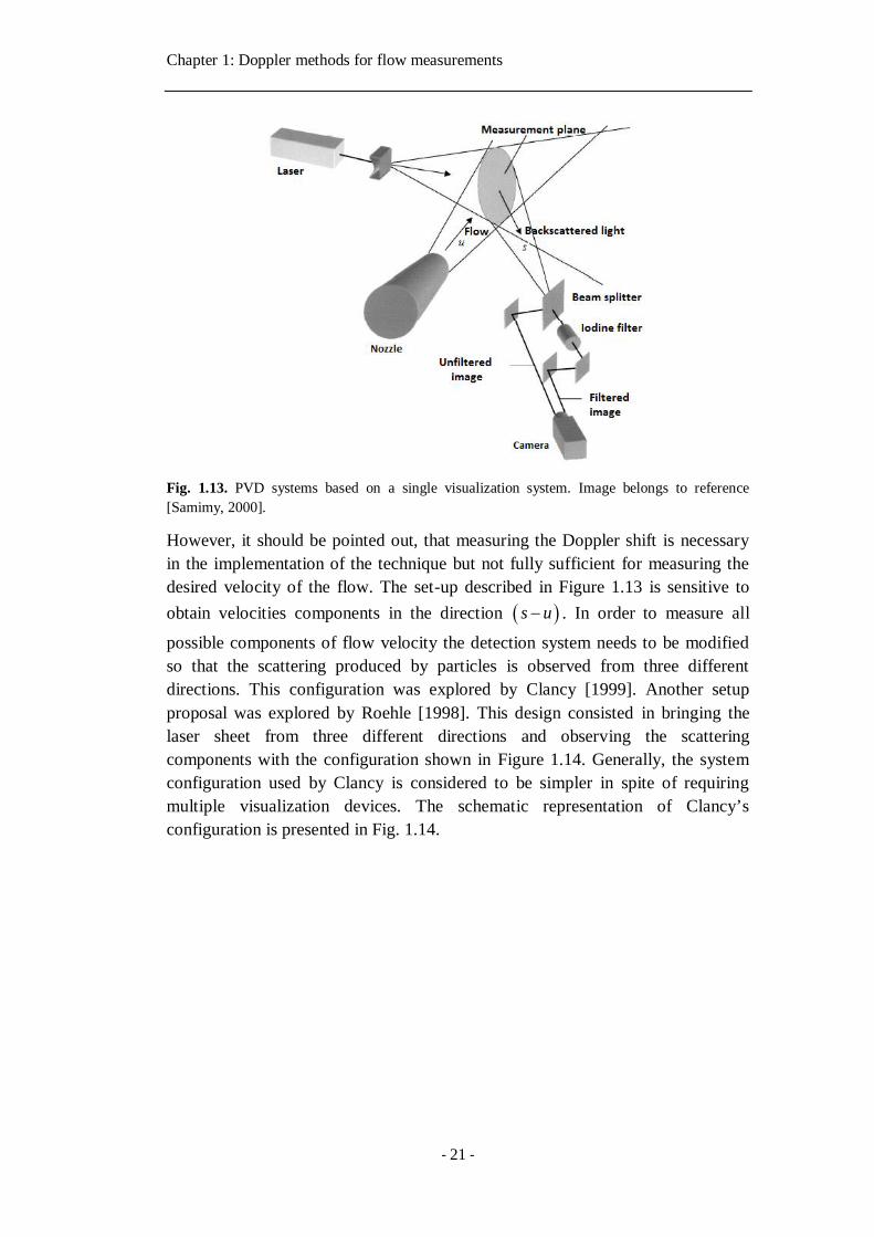
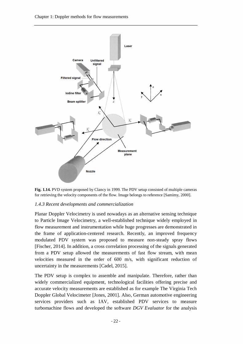
directions. This configuration was explored by Clancy [1999]. Another setup
proposal was explored by Roehle [1998]. This design consisted in bringing the
laser sheet from three different directions and observing the scattering
components with the configuration shown in Figure 1.14. Generally, the system
configuration used by Clancy is considered to be simpler in spite of requiring
multiple visualization devices. The schematic representation of Clancy’s
configuration is presented in Fig. 1.14.
Chapter 1: Doppler methods for flow measurements
- 22 -
Fig. 1.14. PVD system proposed by Clancy in 1999. The PDV setup consisted of multiple cameras
for retrieving the velocity components of the flow. Image belongs to reference [Samimy, 2000].
1.4.3 Recent developments and commercialization
Planar Doppler Velocimetry is used nowadays as an alternative sensing technique
to Particle Image Velocimetry, a well-established technique widely employed in
flow measurement and instrumentation while huge progresses are demonstrated in
the frame of application-centered research. Recently, an improved frequency
modulated PDV system was proposed to measure non-steady spray flows
[Fischer, 2014]. In addition, a cross correlation processing of the signals generated
from a PDV setup allowed the measurements of fast flow stream, with mean
velocities measured in the order of 600 m/s, with significant reduction of
uncertainty in the measurements [Cadel, 2015].
The PDV setup is complex to assemble and manipulate. Therefore, rather than
widely commercialized equipment, technological facilities offering precise and
accurate velocity measurements are established as for example The Virginia Tech
Doppler Global Velocimeter [Jones, 2001]. Also, German automotive engineering
services providers such as IAV, established PDV services to measure
turbomachine flows and developed the software DGV Evaluator for the analysis
Chapter 1: Doppler methods for flow measurements
- 23 -
of the three components of the flow fields. According to Harald Müller from PTB
in Germany, PDV “has become a promising flow field diagnostic tool for research
and development tasks in aerospace and car industry”.
1.5 Three-Component-Doppler-Laser two-focus Velocimetry
1.5.1 Laser two-focus velocimetry
The Laser two-focus (L2F) velocimetry is another method to measure flow
velocity, also known in literature as Laser Transit Anemometry. It shares some
elements with Laser Doppler Velocimetry and Planar Doppler Velocimetry such
as the use of particles merged in the flow and its use in applications with fast
flows.
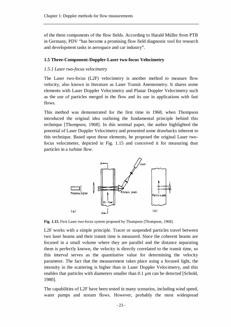
This method was demonstrated for the first time in 1968, when Thompson
introduced the original idea outlining the fundamental principle behind this
technique [Thompson, 1968]. In this seminal paper, the author highlighted the
potential of Laser Doppler Velocimetry and presented some drawbacks inherent to
this technique. Based upon those elements, he proposed the original Laser two-
focus velocimeter, depicted in Fig. 1.15 and conceived it for measuring dust
particles in a turbine flow.
Fig. 1.15. First Laser two-focus system proposed by Thompson [Thompson, 1968].
L2F works with a simple principle. Tracer or suspended particles travel between
two laser beams and their transit time is measured. Since the coherent beams are
focused in a small volume where they are parallel and the distance separating
them is perfectly known, the velocity is directly correlated to the transit time, so
this interval serves as the quantitative value for determining the velocity
parameter. The fact that the measurement takes place using a focused light, the
intensity in the scattering is higher than in Laser Doppler Velocimetry, and this
enables that particles with diameters smaller than 0.1 μm can be detected [Schold,
1980].
The capabilities of L2F have been tested in many scenarios, including wind speed,
water pumps and stream flows. However, probably the most widespread
Chapter 1: Doppler methods for flow measurements
- 24 -
application is in experimental turbomachinery, where it is used in the analysis of
turbulence [Kost, 1997] and vorticity in highly complex flows [Ball, 1988].
However, there are some specific applications where the optical access to flow is
hard and applying L2F to measure three component of velocity is cumbersome or
simple impossible. For those cases, a combination with other techniques is a
reliable solution.
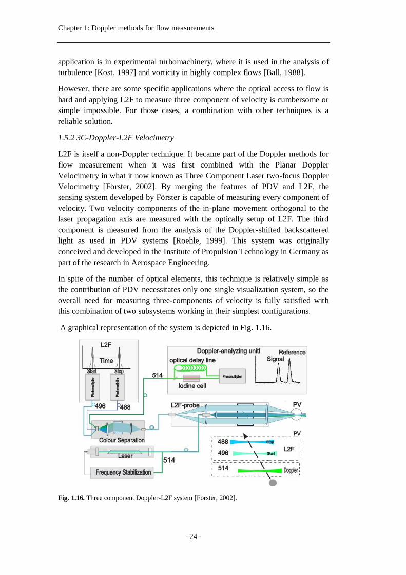
1.5.2 3C-Doppler-L2F Velocimetry
L2F is itself a non-Doppler technique. It became part of the Doppler methods for
flow measurement when it was first combined with the Planar Doppler
Velocimetry in what it now known as Three Component Laser two-focus Doppler
Velocimetry [Förster, 2002]. By merging the features of PDV and L2F, the
sensing system developed by Förster is capable of measuring every component of
velocity. Two velocity components of the in-plane movement orthogonal to the
laser propagation axis are measured with the optically setup of L2F. The third
component is measured from the analysis of the Doppler-shifted backscattered
light as used in PDV systems [Roehle, 1999]. This system was originally
conceived and developed in the Institute of Propulsion Technology in Germany as
part of the research in Aerospace Engineering.
In spite of the number of optical elements, this technique is relatively simple as
the contribution of PDV necessitates only one single visualization system, so the
overall need for measuring three-components of velocity is fully satisfied with
this combination of two subsystems working in their simplest configurations.
A graphical representation of the system is depicted in Fig. 1.16.
Fig. 1.16. Three component Doppler-L2F system [Förster, 2002].
Chapter 1: Doppler methods for flow measurements
- 25 -
1.6 Optical feedback flowmetry
Optical feedback interferometry (OFI) is an interferometric technique with recent
implementation in fluidics and flow measurements. It uses a laser as a sensing
device with minimal optical components. OFI’s physical principle is based on the
interferences generated by the back-scattered light inside the laser’s resonant
cavity to extract information on the sensed object. When used for sensing
purposes in fluidics applications, it is denominated Optical Feedback Flowmetry.
1.6.1 History
The history of optical feedback started almost immediately after the invention of
the laser. In most cases optical feedback, or the self-mixing of an electromagnetic
waves in the laser cavity after being back-scattered by an external object, was
considered as a parasitic effect affecting both laser’s frequency and amplitude.
The first demonstration of the potential capabilities of the technique in sensing
applications started in 1963 with the work of King and Steward [King, 1963;
Hilsum, 1963]. Their articles demonstrated the feasibility of optical feedback to
measure displacement even though as little as 0.1 % of scattered light from an
object distant up to 10 m entered back inside the lasing cavity. In a clear attempt
to extend the utility of the phenomenon of optical feedback in lasers in the general
field of metrology, King and Steward filed a patent application in 1968 that
introduced a general discussion on the potential of optical feedback interferometry
for measuring physical parameters [King, 1968].
During the sixties, optical arrangements where designed and mounted in order to
avoid the effect of external feedback entering back in the resonant cavity of the
laser [Servagent, 1998]. The first application in velocimetry was reported as early
as 1968 when Rudd proposed the first Doppler velocimeter using self-mixing
effect in He-Ne gas laser [Rudd, 1968].
Gas laser were continuously used in the seventies. In 1972, Honeycutt and Otto
reported the utilization of a CO2 laser for range finding [Honeycutt, 1972]. A few
years later, a feedback-induced device was reportedly employed in reading a
compact disc [Seko, 1975]. A self-mixing displacement sensor was proposed by
Donati in 1978 using a combination of analog circuitry with an He-Ne laser
[Donati, 1978].
It was in the eighties when OFI started to be employed in sensors incorporating
semiconductor lasers, thanks to the advent of laser diodes. In 1980, Lang and
Kobayashi [Lang, 1980] conducted a study on the phenomenon of external
feedback in laser diodes and developed the equations ruling the behavior of lasers
while subjected to optical feedback effect. Later on, Shinohara used laser diodes
for velocity measurements [Shinohara, 1986].
Chapter 1: Doppler methods for flow measurements
- 26 -
For many years, optical feedback has been used in diverse scenarios as an
alternative tool allowing precise measurements of vibration, absolute distance and
velocity. OFI’s ability to measure velocity led to its implementation for sensing
purposes in diverse fluidic applications. Koelink and de Mul proposed and
demonstrated the first self-mixing flowmeter in 1992 [Koelink, 1992; de Mul,
1992]. The first optical feedback flow sensor accurately measured the flow
velocity and these measurements were validated with a linear relationship
obtained between flow rate and measured velocity. Since then, OFI sensors have
been tested and implemented in flow assessment in fluidics, microfluidics and
general flowmetry with interest in chemical and biomedical engineering. It has
been employed in the past for measuring blood flow over skin [Özdemir, 2008],
blood perfusion in tissue [de Mul, 1993; Figueiras, 2013] and drop measurements
[Norgia, 2015]. Moreover, this technique is currently being actively employed for
the study of flows in small channels [Campagnolo, 2013] with direct
implementation as an optofluidic alternative sensing technique [Nicolić, 2013].
1.6.2 Sensing principle
Optical feedback interferometry uses a reinjection scheme. Light emitted by a
laser impinges in a moving target and a part of the scattered light is fed back
inside the laser cavity. This reinjection causes variations in the laser emission
power and junction voltage that can be employed to obtain information on the
target and describe kinematic features of the external object such as its velocity or
vibration frequency.
In Optical Feedback Flowmetry, the external feedback is generated by particles
flowing in a fluid. Light scattered by those tracer particles enters back in the laser
and modulate its lasing properties. As in Laser Doppler Velocimetry, this Doppler
frequency 𝑓𝐷 is related to the particle’s velocity as explained in expression 1.6.
The fundamental aspects of OFI’s sensing scheme will be exposed throughout this
thesis. Thereby, it will be provided the basics of the phenomenon behind this
technique as well as applications in sensing and interrogation of fluid flows.
1.6.3 Particular features of optical feedback interferometry
In OFI based sensing systems, a laser is used as the light source, interferometer
and receiver and for many applications very few optical components are needed.
This makes OFI sensors generally compact when compared to other sensing
devices. Other advantages include its self-alignment, thus avoiding complex
alignments required by classical interferometry. In addition, taking advantages
from the light amplification in the laser cavity where the interferences take place,
OFI is sensitive to very low levels of back-scattered optical power.
OFI can be considered as a consolidated and mature interferometric technique in
mechatronics, typically for velocity, vibration and displacement measurements
Chapter 1: Doppler methods for flow measurements
- 27 -
[Atashkhooei, 2014; Arriaga, 2016] and as an alternative method for multiple
biomedical studies [Donati, 2014; Bakar, 2013]. A recent review summarizes
most of the known applications [Taimre, 2015]. Moreover, current trends in OFI’s
implementation for multiple biomedical applications are described in a recent
publication [Perchoux, 2016].
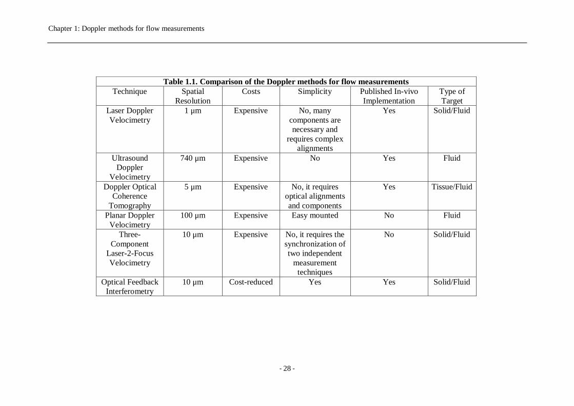
1.7 Comparison of the methods and key features
The main features of the techniques presented in this chapter are outlined in Table
1. Key parameters inherent to the measurement scheme utilized by the detection
system are detailed in terms of technical and economic relevance. To this end, this
table provides a general overview of the advantages and constraints relative to the
Doppler measurement techniques used in fluid flow assessment and
quantification.
LDV and ODT perform accurate velocity measurements with high resolution.
This is particularly interesting as this resolution is comparable to the typical
resolution that optical feedback interferometry sensors hold for many applications
in fluid flow measurements, which is utmost important for sensing at the
microscale. However, both LDV and ODT require complex optical arrangements
resulting in bulky equipment that makes complicated its direct implementation for
microscale fluid measurements.
Ultrasound Doppler flowmetry measures flow velocity in channels and pipes
without direct dependence on the transparency of the flowchannel, thus it can
perform valid measurements where the rest of the optical methods exposed in this
chapter may not. However, this technique has the drawback that it does not offer
high resolution in the measurements when compared to the characteristic
resolution of the optical Doppler methods reviewed here.
Finally, PDV and 3C-L2F velocimetry are complicated to be implemented,
difficult to mount and require many optical and visualization components.
However, these techniques are capable or measuring with good accuracy and
resolutions comparable to that of OFI systems.
Chapter 1: Doppler methods for flow measurements
- 28 -
Table 1.1. Comparison of the Doppler methods for flow measurements
Technique Spatial
Resolution
Costs Simplicity Published In-vivo
Implementation
Type of
Target
Laser Doppler
Velocimetry
1 μm Expensive No, many
components are
necessary and
requires complex
alignments
Yes Solid/Fluid
Ultrasound
Doppler
Velocimetry
740 μm Expensive No Yes Fluid
Doppler Optical
Coherence
Tomography
5 μm Expensive No, it requires
optical alignments
and components
Yes Tissue/Fluid
Planar Doppler
Velocimetry
100 μm Expensive Easy mounted No Fluid
Three-
Component
Laser-2-Focus
Velocimetry
10 μm Expensive No, it requires the
synchronization of
two independent
measurement
techniques
No Solid/Fluid
Optical Feedback
Interferometry
10 μm Cost-reduced Yes Yes Solid/Fluid
Chapter 1: Doppler methods for flow measurements
- 29 -
1.8 Motivations of the present thesis
Optical feedback interferometry, as any other interferometric technique, is limited
in the detection scheme and consequently in sensing applications. One can
mention, for example, the impact of speckle effect in the amplitude of self-mixing
signals, the susceptibility of signals to extraneous parasitic vibrations and
therefore, the complexity of designing optical feedback sensors for compensation
of externally affected signals to successfully retrieve the displacement when
measuring vibrations. These issues were subject of research of several authors
extensively addressed in their thesis dissertations [Arriaga, 2014a; Zabit, 2010]
In the case of optical feedback flowmetry, the signal processing may vary
depending on the concentration of particles in the sensing volume. It is distinctive
the shape of the spectrum at low particle concentration, the so-called single
scattering regime, as compared to the power spectral density of highly
concentrated particles, the multiple scattering regime. So, it is of great interest to
study when a particular signal processing is suitable for sensing in one regime or
the other, and the reliability of each signal processing in in-situ sensing
applications. Throughout this thesis, we drive our attention at exploring
experimentally the optical feedback flowmetry in both single and multiple
scattering regime to further discern when a signal processing can successfully
sense in either regime.
In an effort to conceive OFI-based online measurements, we explored the
capabilities of this technique in detecting suspended monoparticle in microfluidic
devices. We propose a methodology enabling particle tracking, localization and
size estimation. Single particle detection is the extreme limit of detection in the
single scattering regime, where signal processing is straightforward.
Taking advantages of the fact that signal processing associated to the single
scattering regime in optical feedback flowmetry is relatively simple, we have
performed a study on the ability of OFI sensors in ex-vivo characterization of
flow inside a vessel, which is proposed as pressure myograph sytem useful to
investigate hemodynamics in microcirculation.
Being able to sense in single or multiple scattering extends the utility of optical
feedback interferometry sensors in fluidics applications in both micro and
macroscale, thus providing the chemical, biomedical and biotechnological
industry with new alternative non-contact, non-destructive tool utilizing only a
laser for sensing purposes.
As part of this thesis dissertation, we developed an OFI sensor allowing the
analysis of non-steady flows in the multiple scattering regime. Unsteady flows are
present in many cases in industry
Chapter 1: Doppler methods for flow measurements
- 30 -
Also, proposing this kind of sensors for the assessment of multiphase flows is of
actual relevance as most of the experimentation in this regard depends strongly on
visualization systems. We extensively explore OFI for the interrogation of two-
phase immiscible liquid-liquid interactions using the flow profile characterization
from parameters of fluid motion. This is a first step in the implementation of OFI
sensors in the analysis of two-phase flows, which has been up to now unexplored.
Chapter 2: Optical feedback interferometry for flows: theoretical fundaments
- 31 -
Chapter 2
Optical feedback interferometry for flows: theoretical fundaments
In this chapter, we present the different scattering mechanisms that are present as
a consequence of the interaction of the laser used in the optical feedback
interferometry sensing technique with a moving target. We focus our attention
towards the implications of the nature of the target on the optical feedback
departing from the main theoretical fundaments of on which the phenomenon is
based applied to semiconductor lasers.
When the laser light interacts with a moving object, part of the backscattered
radiation re-enters the laser cavity and mix with the original emitted wave. Due to
the Doppler Effect, this reinjection in the laser affects directly its emission power
and spectral properties. The amplitude and frequency fluctuations are due to a
“parasite” feedback, other than the feedback by the mirrors of the laser resonator,
caused by reflection (diffuse or not) on external surfaces.
In what follows, we examine the optical feedback in the case of the interaction of
the laser beam with flowing particles in a fluid, and its impact in the behavior of
the laser subject to feedback generated by those particles.
Chapter 2: Optical feedback interferometry for flows: theoretical fundaments
- 32 -
2.1 Optical feedback phenomenon for flow measurements
Optical feedback interferometry has been extensively studied and applied in
mechatronics. However, its implementation in fluid flow measurement systems is
rather recent. Most of the work developed to implement OFI sensors in fluidics
circumscribes in the frame of velocimetry. Still, measuring velocity with accuracy
is challenging and at the same time an increasing need for the biomedical,
chemical and industrial communities.
Unlike solid targets, light scattered by small particles in a flow generate a
diffusion pattern where the scattered electromagnetic field vectors are randomly
distributed all over a round solid angle. Typically in solid targets light is scattered
preferentially in the direction of the laser beam propagation.
This section presents the basic principles of OFI applied to velocity measurements
of flows. The main features of the interaction of the laser beam with the carrying
scattering particles are posed and analyzed.
2.1.1 Particular features of the interaction laser-fluid
The sensing mechanism of the optical feedback interferometry technique applied
to flow measurements depends on the interaction of a laser beam and the particles
embedded in the flow. There are particular features that models and
approximations need to consider. The following aspects are distinctive:
- Light travels through a gradient of refractive indexes as it passes from
different materials until it reaches the particles in the flow.
- Many particles in the flow may be illuminated at once; hence the
contribution to the optical feedback signal has a frequency signature
characterized by a distribution of frequencies correlated to a plurality of
particles travelling at different velocities.
- The illuminated volume where particles in the flow contribute to the
optical feedback affecting the laser has three dimensional spatial
components.
- The scattering angle is 2π. This means that light is scattered in all
directions, not only in the direction towards the laser as in the case of solid
targets. This implies that the detection of light from fluidic systems
interrogated by optical feedback interferometry is poor with respect to the
sensing of solid targets.
It is important to take into consideration also that particles may behave different
from the fluid so that they do not follow perfectly the flow hydrodynamics.
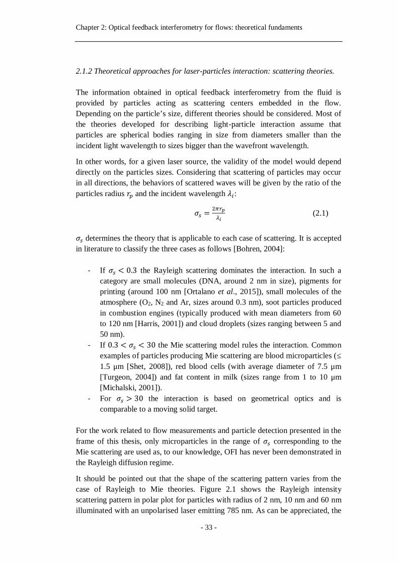
Chapter 2: Optical feedback interferometry for flows: theoretical fundaments
- 33 -
2.1.2 Theoretical approaches for laser-particles interaction: scattering theories.
The information obtained in optical feedback interferometry from the fluid is
provided by particles acting as scattering centers embedded in the flow.
Depending on the particle’s size, different theories should be considered. Most of
the theories developed for describing light-particle interaction assume that
particles are spherical bodies ranging in size from diameters smaller than the
incident light wavelength to sizes bigger than the wavefront wavelength.
In other words, for a given laser source, the validity of the model would depend
directly on the particles sizes. Considering that scattering of particles may occur
in all directions, the behaviors of scattered waves will be given by the ratio of the
particles radius 𝑟𝑝 and the incident wavelength 𝜆𝑖:
𝜎𝑠 =2𝜋𝑟𝑝
𝜆𝑖 (2.1)
𝜎𝑠 determines the theory that is applicable to each case of scattering. It is accepted
in literature to classify the three cases as follows [Bohren, 2004]:
- If 𝜎𝑠 < 0.3 the Rayleigh scattering dominates the interaction. In such a
category are small molecules (DNA, around 2 nm in size), pigments for
printing (around 100 nm [Ortalano et al., 2015]), small molecules of the
atmosphere (O2, N2 and Ar, sizes around 0.3 nm), soot particles produced
in combustion engines (typically produced with mean diameters from 60
to 120 nm [Harris, 2001]) and cloud droplets (sizes ranging between 5 and
50 nm).
- If 0.3 < 𝜎𝑠 < 30 the Mie scattering model rules the interaction. Common
examples of particles producing Mie scattering are blood microparticles (≤
1.5 μm [Shet, 2008]), red blood cells (with average diameter of 7.5 μm
[Turgeon, 2004]) and fat content in milk (sizes range from 1 to 10 μm
[Michalski, 2001]).
- For 𝜎𝑠 > 30 the interaction is based on geometrical optics and is
comparable to a moving solid target.
For the work related to flow measurements and particle detection presented in the
frame of this thesis, only microparticles in the range of 𝜎𝑠 corresponding to the
Mie scattering are used as, to our knowledge, OFI has never been demonstrated in
the Rayleigh diffusion regime.
It should be pointed out that the shape of the scattering pattern varies from the
case of Rayleigh to Mie theories. Figure 2.1 shows the Rayleigh intensity
scattering pattern in polar plot for particles with radius of 2 nm, 10 nm and 60 nm
illuminated with an unpolarised laser emitting 785 nm. As can be appreciated, the
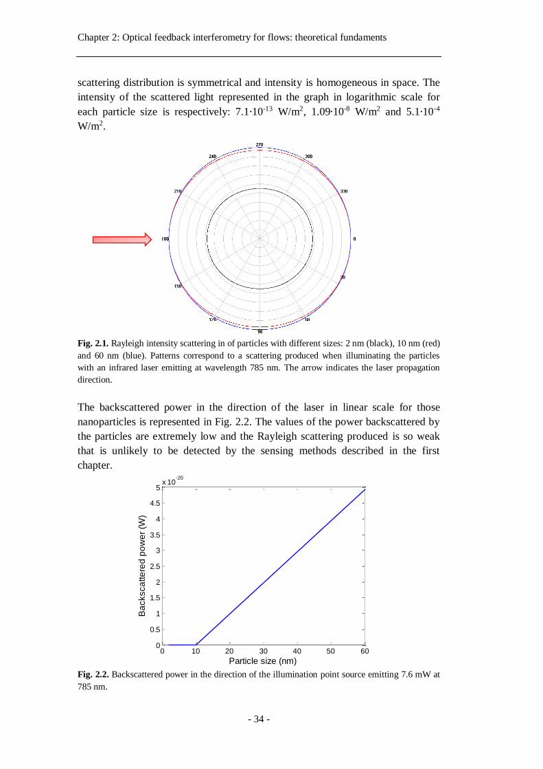
Chapter 2: Optical feedback interferometry for flows: theoretical fundaments
- 34 -
scattering distribution is symmetrical and intensity is homogeneous in space. The
intensity of the scattered light represented in the graph in logarithmic scale for
each particle size is respectively: 7.1∙10-13 W/m2, 1.09∙10-8 W/m2 and 5.1∙10-4
W/m2.
Fig. 2.1. Rayleigh intensity scattering in of particles with different sizes: 2 nm (black), 10 nm (red)
and 60 nm (blue). Patterns correspond to a scattering produced when illuminating the particles
with an infrared laser emitting at wavelength 785 nm. The arrow indicates the laser propagation
direction.
The backscattered power in the direction of the laser in linear scale for those
nanoparticles is represented in Fig. 2.2. The values of the power backscattered by
the particles are extremely low and the Rayleigh scattering produced is so weak
that is unlikely to be detected by the sensing methods described in the first
chapter.
Fig. 2.2. Backscattered power in the direction of the illumination point source emitting 7.6 mW at
785 nm.
0 10 20 30 40 50 600
0.5
1
1.5
2
2.5
3
3.5
4
4.5
5x 10
-20
Ba
cksca
tte
red
po
we
r (W
)
Particle size (nm)
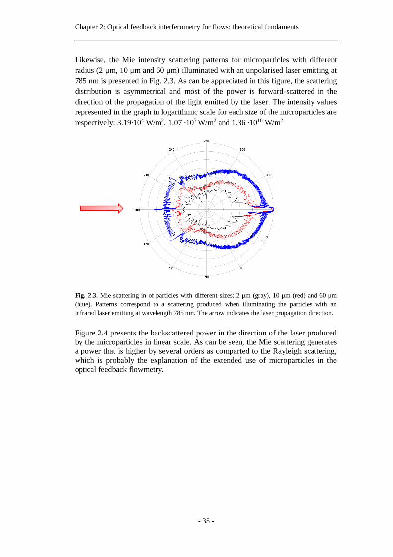
Chapter 2: Optical feedback interferometry for flows: theoretical fundaments
- 35 -
Likewise, the Mie intensity scattering patterns for microparticles with different
radius (2 μm, 10 μm and 60 μm) illuminated with an unpolarised laser emitting at
785 nm is presented in Fig. 2.3. As can be appreciated in this figure, the scattering
distribution is asymmetrical and most of the power is forward-scattered in the
direction of the propagation of the light emitted by the laser. The intensity values
represented in the graph in logarithmic scale for each size of the microparticles are
respectively: 3.19∙104 W/m2, 1.07 ∙107 W/m2 and 1.36 ∙1010 W/m2
Fig. 2.3. Mie scattering in of particles with different sizes: 2 μm (gray), 10 μm (red) and 60 μm
(blue). Patterns correspond to a scattering produced when illuminating the particles with an
infrared laser emitting at wavelength 785 nm. The arrow indicates the laser propagation direction.
Figure 2.4 presents the backscattered power in the direction of the laser produced
by the microparticles in linear scale. As can be seen, the Mie scattering generates
a power that is higher by several orders as comparted to the Rayleigh scattering,
which is probably the explanation of the extended use of microparticles in the
optical feedback flowmetry.
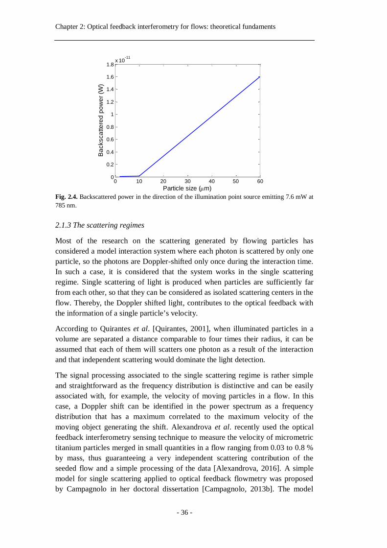
Chapter 2: Optical feedback interferometry for flows: theoretical fundaments
- 36 -
Fig. 2.4. Backscattered power in the direction of the illumination point source emitting 7.6 mW at
785 nm.
2.1.3 The scattering regimes
Most of the research on the scattering generated by flowing particles has
considered a model interaction system where each photon is scattered by only one
particle, so the photons are Doppler-shifted only once during the interaction time.
In such a case, it is considered that the system works in the single scattering
regime. Single scattering of light is produced when particles are sufficiently far
from each other, so that they can be considered as isolated scattering centers in the
flow. Thereby, the Doppler shifted light, contributes to the optical feedback with
the information of a single particle’s velocity.
According to Quirantes et al. [Quirantes, 2001], when illuminated particles in a
volume are separated a distance comparable to four times their radius, it can be
assumed that each of them will scatters one photon as a result of the interaction
and that independent scattering would dominate the light detection.
The signal processing associated to the single scattering regime is rather simple
and straightforward as the frequency distribution is distinctive and can be easily
associated with, for example, the velocity of moving particles in a flow. In this
case, a Doppler shift can be identified in the power spectrum as a frequency
distribution that has a maximum correlated to the maximum velocity of the
moving object generating the shift. Alexandrova et al. recently used the optical
feedback interferometry sensing technique to measure the velocity of micrometric
titanium particles merged in small quantities in a flow ranging from 0.03 to 0.8 %
by mass, thus guaranteeing a very independent scattering contribution of the
seeded flow and a simple processing of the data [Alexandrova, 2016]. A simple
model for single scattering applied to optical feedback flowmetry was proposed
by Campagnolo in her doctoral dissertation [Campagnolo, 2013b]. The model
0 10 20 30 40 50 600
0.2
0.4
0.6
0.8
1
1.2
1.4
1.6
1.8x 10
-11
Particle size (m)
Ba
cksca
tte
red
po
we
r (W
)
Chapter 2: Optical feedback interferometry for flows: theoretical fundaments
- 37 -
reproduced the power spectrum of a fluid moving at a given known flow rate
using the equivalent reflection coefficient from the theory optical feedback.
If the number of obstacles in a medium where light propagates is large, then the
wave interacts multiple times with the bodies in the medium. In this case, the
phenomenology is understood as an interaction process in the multiple scattering
regime. Perhaps the closest example attributable to a sensing scheme in the
multiple scattering regime is the measurement of blood perfusion in tissue and the
measurement of blood flow in veins and arteries. Also, many experiments use
phantoms based on milk or intralipid to mimic light interaction with living tissue.
I this regard, many techniques devoted to measure any activity related to the tissue
use the Doppler Effect to retrieve information on the flow, perfusion and
microcirculation.
The multiple scattering regime in the case of a laser impinging a medium with
flowing particles is applicable when in the concentration of scatterers is high and
photons experience multiple reflections with the particles in the medium and they
suffer several Doppler shifts before they propagate towards the laser cavity. In
this case, the spectral properties of the optical feedback signal are highly random
and the frequency distribution has a complex statistical behavior. The multiple
scattering effect is a complex phenomenon involving random interactions between
the light wave and matter that has been addressed by different approaches
depending on the nature of the scattering particles. As explained in the previous
section, the size of the particles influences the scattering pattern associated to the
type of interaction. However, the problem of retrieving the quantitative
information of moving particles has been a major challenge using different
techniques in the multiple scattering regime such as laser speckle contrast imaging
and Doppler optical coherence tomography.
A scattering model presented by Bonner et al. [Bonner, 1981] proposed to
consider the spectrum of the time autocorrelation function of detected photons
experiencing multiple collisions in a tissue as it is related to the scattering
function. The normalized scattering function is composed of the sum the product
of the probability that photons undergo several collision on the tissue and the
autocorrelation function for an equal number of collisions. Then, for a wave
interacting with the medium, the center of mass of the moving scatterers is
continuously changing and as a consequence, the wave is Doppler-shifted. The
model yielded a direct relation of the first order moment of the spectrum with the
radius of the particles in the flow, the velocity of the scattering centers and the
number of particles generating scattering. This physical approximation allows for
the interpretation of the mean frequency of a spectrum. The signal's spectrum can
be assimilated as a probability density function related to the velocity of particles
embedded in the flow. Those particles scatter a portion of the incident light, which
is Doppler shifted. By summing up the contribution of each interaction the mean
Chapter 2: Optical feedback interferometry for flows: theoretical fundaments
- 38 -
frequency can be calculated from the center of mass of the power spectrum. The
sense of the center of mass of a frequency distribution was exploited by de Mul et
al. in the development of an instrument to measure directly the blood flow
velocity [de Mul, 1984]. In addition, Nilsson conceived and developed a signal
processor for flow measurement [Nilsson, 1984] and Norgia et al. measured
extracorporeal flows using the same principle [Norgia, 2010].
Using Monte Carlo simulations Davis et al. studied the photon propagation in
tissue with vasculatures and the implications of multiple scattering in the
interpretation of the laser speckle contrast imaging (LSCI) [Davis, 2014]. LSCI
uses backscattered light to image a changing structure that generates a blurring
effect in those regions with flow or evident microcirculation associated. They
found that a large percent of photons, more than 75 %, experience multiple
scattering for various values of the scattering coefficient. Their work,
demonstrated that existing models that consider only single scattering in
functional vessels may fall into a wrong approximation for blood flow assessment.
The effects of multiple scattering are associated to the interaction of the light
source with the moving elements in the flow. However, multiple scattering arises
as light propagates through a medium before interacting with the flow stream.
Moger et al. analyzed the effect of multiple scattering in the velocity profile of
blood measured by Doppler optical coherence tomography [Moger, 2005]. Their
study consisted on mimicking a flow under a high-scattering medium by adding
phantoms with different thickness. In this way, it is possible to measure the
influence of the scattering regime in the ability of the technique to measure the
velocity in depth by immersing the tube carrying the fluid in water and in a 20 %
solution of intralipid. The comparative results concluded that for a scattering layer
of intralipid thicker than 150 μm, multiple scattering effects introduce systematic
errors in the measured velocity profile and rigorous fitting needs to be performed
to accurately fit the experimental results with an analytical expression of the
profile.
Kalkman et al. investigated the effect of multiple scattering of blood in the
Doppler OCT using different dilutions of hematocrit ranging from 0 % to 15 %
[Kalkman, 2012]. From a set of Monte Carlo simulations of the ODT signals, they
explained the influence of multiple scattering and the scattering anisotropy in
signals for blood flowing in a cuvette. The simulations considered the sum of all
photons and the contributions of several scattering events in the sample. Good
coincidence was found between their simulation outcomes and the experimental
results, which demonstrated that photons may experience more than 20 scattering
events in the flow.
As multiple scattering effects are complex, the use of high concentration of
particles in liquids is usually avoided as much as possible [Kliese, 2010;
Campagnolo, 2013a; Norgia, 2012]. Doppler methods take advantage of the
Chapter 2: Optical feedback interferometry for flows: theoretical fundaments
- 39 -
relatively simpler processing of the data in the single scattering regime. In many
cases, the theoretical framework present in the literature is limited to flow sensing
in the single scattering regime and assuming that multiple scattering effects are
negligible. In addition, very few is found in literature to explain how the multiple
scattering effect may impact the measurement of velocity using Doppler methods.
While there is an ongoing active research in scattering models and how they
would fairly reproduce the information observed in the experiments, we will focus
on presenting the working principle of the optical feedback interferometry sensors
for flow measurements in the following section and we will address
experimentally the potential applications of the single scattering in the third and
fourth chapter of the present thesis and present a processing analysis from single
to multiple scattering in the third chapter.
2.2 Theory of the optical feedback applied to multiple scatterers
In this section, the fundamental equations of the laser under external feedback are
presented and the model is developed to determine the impact of multiple
scatterers to the laser amplitude changes.
Two options are possible to describe the behavior of the laser diode under optical
feedback: first, the three mirror cavity (the third mirror being the target) can be
reduced to a two-mirror equivalent cavity from which the laser rate equations can
be deduced [Petermann, 1991]; second, the optical feedback can be seen as a
perturbation of the established lasing systems and, in this case, an additional term
can directly be added to the field or photon rate equation that represents the
contribution of the back-scattered light. This second way is known as the Lang
and Kobayashi model [Lang, 1980]. A discussion on the advantages and the
inconveniences of both modeling methods is presented in [Kane, 2007]. The
conclusion of this study shows that, despite the equivalent cavity method is the
most exact method, the Lang and Kobayashi perturbation approach is well suited
for low feedback levels and quasi steady state analysis of the optical feedback
phenomenon.
In the case where the optical feedback is due to small particles flowing in fluids,
where the back-scattered power is described by the Mie theory, the optical
feedback level remains very low. Despite Campagnolo [Campagnolo, 2013] has
demonstrated the contribution of multiple scatterers based on the equivalent cavity
model, we have derived the Lang-Kobayashi method as originally proposed by
Zakian [Zakian, 2005].
The modeling approach is based on the description of the established electric field
propagating inside the laser cavity E that is subject to an external perturbation:
Chapter 2: Optical feedback interferometry for flows: theoretical fundaments
- 40 -
d
d𝑡[𝐸(𝑡) exp(j𝜔𝑡)] = [j𝜔𝑁 +
1
2Γ𝐺(𝑁 − 𝑁tr)] 𝐸(𝑡) exp(j𝜔𝑡) + 𝑭(𝒕) (2.2)
where 𝜔 is the laser mode angular frequency, 𝜔𝑁 is the cavity mode angular
frequency (𝜔𝑁 = 𝑘𝜋𝑐/𝑛𝑐𝐿𝑐 with k an integer, 𝐿𝑐 the laser cavity length and 𝑛𝑐
the refractive index), Γ stands for the laser mode confinement factor, N is the
carrier density, 𝑁tr is the carrier density at transparency, G is the stimulated
emission gain and F(t) is the feedback induced perturbation term. Depending on
the nature of the target, F(t) can adopt different formulations :
- In the case of a unique and fixed target located at a distance 𝐿ext from the
laser cavity,
𝐹(𝑡) =𝜅
𝜏𝐶𝐸(𝑡 − 𝜏) exp[jω(𝑡 − 𝜏)], (2.3)
where 𝜏 is the external cavity roundtrip time of flight (𝜏 = 2𝑛ext𝐿ext/𝑐),
𝜏𝑐 is the laser cavity roundtrip time of flight (𝜏𝐶 = 2𝑛𝐶𝐿𝐶/𝑐) and 𝜅 is the
feedback coupling coefficient defined as
𝜅 =1
𝜏𝐶(1 − 𝑟2
2)𝑟ext
𝑟2 (2.4)
with 𝑟2 the reflectivity of the laser front mirror and 𝑟ext the ratio of the
back-scattered power actually re-entering the laser cavity over the emitted
power.
- In the case of a unique target in translation that induces a Doppler shift
𝑓𝐷 =𝜔𝐷
2𝜋=
𝜔
2𝜋
2𝑉
𝑐 + 𝑉 (2.5)
is dependent on the target’s velocity V and the feedback contribution
becomes
𝐹(𝑡) =𝜅
𝜏𝐶𝐸(𝑡 − 𝜏) exp[j(𝜔 + 𝜔𝐷)(𝑡 − 𝜏)]. (2.6)
- In the case of multiple targets, each one scatters back toward the laser
cavity its own contribution so that:
𝐹(𝑡) = ∑ 𝐹𝑖(𝑡)
𝑖
, (2.7)
with each 𝐹𝑖(𝑡) that can be written as :
𝐹𝑖(𝑡) =𝜅𝑖
𝜏𝐶𝐸(𝑡 − 𝜏𝑖) exp[j(𝜔 + 𝜔𝐷,𝑖)(𝑡 − 𝜏𝑖)] (2.8)
Chapter 2: Optical feedback interferometry for flows: theoretical fundaments
- 41 -
That takes into account the fact that each particle is located at a specific
distance from the target which induces a particular time of flight 𝜏𝑖, that
the reflectivity of each particle is its proper characteristic so that
𝜅𝑖 =1
𝜏𝐶
(1 − 𝑟22)
𝑟ext,𝑖
𝑟2, (2.9)
and that each particle has its proper velocity projection along the optical
axis inducing
𝜔𝐷,𝑖 = 𝜔2𝑉𝑖
𝑐 + 𝑉𝑖. (2.10)
Thus considering equation (2.2) with the perturbation F(t) described as (2.8)
obtaining the variation of the laser output power induced by the particle optical
feedback consists in solving the set of rate equations that describe the laser by
separating the real and the imaginary part of the field equation and introducing the
carrier density equation. In the meantime, considering the Doppler shift induced
by the particle velocity is at very low frequency when compared to the laser
optical frequency, the usual approximations of the quasi-steady state regime can
be done : 𝐸(𝑡 − 𝜏)~𝐸(𝑡), thus :
d𝐸(𝑡)
d𝑡=
1
2Γ𝐺(𝑁 − 𝑁tr)𝐸(𝑡) + ∑
𝜅𝑖
𝜏𝐶𝐸(𝑡) cos(𝜔𝐷,𝑖𝑡 + 𝜙𝑖)
𝑖
, (2.11)
d𝛷(𝑡)
d𝑡=
1
2𝛼Γ𝐺(𝑁 − 𝑁tr) + ∑
𝜅𝑖
𝜏𝐶sin(𝜔𝐷,𝑖𝑡 + 𝜙𝑖)
𝑖
, (2.12)
d𝑁(𝑡)
d𝑡=
𝐼
𝑞𝑉𝑎− 𝐺(𝑁 − 𝑁tr)𝑆 −
𝑁
𝜏𝑛, (2.13)
where 𝛼 is the linewidth enhancement factor, 𝛷 is the phase term of the electric
field E, 𝜙𝑖 is a random phase, q is the elementary charge, 𝑉𝑎 is the laser active
volume, 𝜏𝑛 is the carrier lifetime and S is the photon density which is linked to the
field amplitude by :
𝑆 ∝ 𝐸 ∙ 𝐸∗, (2.14)
which allows to re-write (2.11) as
d𝑆(𝑡)
d𝑡= 𝐺(𝑁 − 𝑁th)𝑆(𝑡) −
𝑆(𝑡)
𝜏𝑆+ ∑
𝜅𝑖
𝜏𝐶𝑆(𝑡) cos(𝜔𝐷,𝑖𝑡 + 𝜙𝑖)
𝑖
, (2.15)
In (2.15), 𝜏𝑆 is the photon lifetime and 𝑁th is the carrier density at threshold.
Solving the set of equations (2.11)-(2.15) in the case of the quasi-steady state
regime has been exposed in many ways [Kane, 2005], [Taimre, 2015]. Following
the exact same methodology leads to write the following equations for phase and
amplitude respectively:
Chapter 2: Optical feedback interferometry for flows: theoretical fundaments
- 42 -
𝜔𝐹 − 𝜔0 = 𝛼 ∑𝜅𝑖
𝜏𝐶cos(𝜔𝐷,𝑖𝑡 + 𝜙𝑖) + ∑
𝜅𝑖
𝜏𝐶sin(𝜔𝐷,𝑖𝑡 + 𝜙𝑖)
𝑖𝑖
, (2.16)
𝑆𝐹 = 𝑆0 [1 + 2𝜏𝑆
𝜏𝐶∑ 𝜅𝑖cos(𝜔𝐷,𝑖𝑡 + 𝜙𝑖)
𝑖
] (2.17)
where 𝜔𝐹 and 𝜔0 are the laser angular frequency with and without feedback
respectively and 𝑆𝐹 and 𝑆0 are the photon densities under similar hypothesis.
Eq. (2.16) can be simplified in
𝜔𝐹 − 𝜔0 = √1 + 𝛼2 ∑𝜅𝑖
𝜏𝐶sin(𝜔𝐷,𝑖𝑡 + 𝜙𝑖 + arctan 𝛼)
𝑖
, (2.18)
while (2.17) directly provides a simple and easy relationship for the laser emitted
power variations that are proportional to the photon density
𝑃𝐹 = 𝑃0 [1 + ∑ 𝑚𝑖cos(𝜔𝐷,𝑖𝑡 + 𝜙𝑖)
𝑖
], (2.19)
where the 𝑚𝑖 is the modulation indexes relative to the ith particle:
𝑚𝑖 = 2𝜏𝑆
𝜏𝐶𝜅𝑖 . (2.20)
It shall be noted that despite the Doppler shift 𝜔𝐷,𝑖 is function of 𝜔𝐹 , in the case
of optical feedback in fluids where the low back-scattered power requires a short
range of operation (usually a tens of millimeters), the changes in laser frequency
can be neglected for the calculation of the optical power variations.
To validate the model, the equation (2.19) has been implemented with MatlabTM
for a 1D - distribution of velocities along the optical axis that follows Poiseuille’s
law for velocity distribution in a circular duct (Fig. 2.5(a)). The laser and target
parameters for simulation are presented in the table 1. The flow parameters are as
follows: the maximum velocity in the 320 µm diameter channel is 0.1 m/s, the
flow direction makes an angle of 80° with the optical axis. The light absorption in
the fluid has been fixed so that the penetration depth is 1 mm. A random phase 𝜙𝑖
has been given for each position as originally proposed by Nikolić et al. [Nikolić,
2014] that takes into account both the phase shift induced by the time of flight in
the external cavity and the random phase shift induced by the scattering effect on
the particle. Also, for sake of understanding of the signal spectrum a white
Gaussian noise has been added to the signal through Matlab’s rand function.
As expected the time domain signal presented in Fig. 2.5(b) is clearly not
deterministic and the unique manner to obtain the information on the velocity of
the fluid is the spectral analysis. The flow maximum velocity, considering the
incident angle and the laser wavelength is expected to produce a Doppler shift of
44.2 kHz which corresponds roughly to the maximum observed frequency in the
distributed spectrum of Fig. 2.5(c).
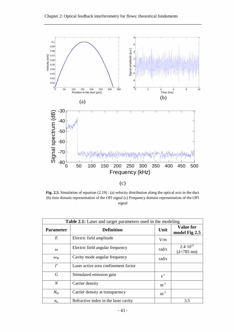
Chapter 2: Optical feedback interferometry for flows: theoretical fundaments
- 43 -
(a) (b)
(c)
Fig. 2.5. Simulation of equation (2.19) : (a) velocity distribution along the optical axis in the duct
(b) time domain representation of the OFI signal (c) Frequency domain representation of the OFI
signal
Table 2.1: Laser and target parameters used in the modeling
Parameter Definition Unit Value for
model Fig 2.5 E Electric field amplitude V/m
𝜔 Electric field angular frequency rad/s 2.4·1015
(𝜆=785 nm)
𝜔𝑁 Cavity mode angular frequency rad/s
𝛤 Laser active area confinement factor
G Stimulated emission gain s-1
N Carrier density m-3
𝑁tr Carrier density at transparency m-3
𝑛𝑐 Refractive index in the laser cavity 3.5
0 50 100 150 200 250 300 3500
0.01
0.02
0.03
0.04
0.05
0.06
0.07
0.08
0.09
0.1
Position in the duct (µm)
Ve
locity (
m/s
)
0 2 4 6 8 10-6
-4
-2
0
2
4
6
8
Time (ms)
Sig
na
l a
mp
litu
de
(a
.u.)
0 50 100 150 200 250 300 350 400 450 500-80
-70
-60
-50
-40
-30
Frequency (kHz)
Sig
na
l sp
ectr
um
(d
B)
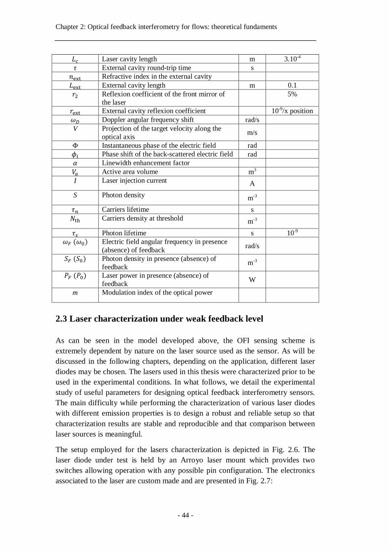
Chapter 2: Optical feedback interferometry for flows: theoretical fundaments
- 44 -
𝐿𝑐 Laser cavity length m 3.10-4
𝜏 External cavity round-trip time s
𝑛ext Refractive index in the external cavity
𝐿ext External cavity length m 0.1
𝑟2 Reflexion coefficient of the front mirror of
the laser
5%
𝑟ext External cavity reflexion coefficient 10-9/x position
𝜔𝐷 Doppler angular frequency shift rad/s
V Projection of the target velocity along the
optical axis m/s
Φ Instantaneous phase of the electric field rad
𝜙𝑖 Phase shift of the back-scattered electric field rad
𝛼 Linewidth enhancement factor
𝑉𝑎 Active area volume m3
I Laser injection current A
S Photon density m-3
𝜏𝑛 Carriers lifetime s
𝑁th Carriers density at threshold m-3
𝜏𝑠 Photon lifetime s 10-9
𝜔𝐹 (𝜔0) Electric field angular frequency in presence
(absence) of feedback rad/s
𝑆𝐹 (𝑆0) Photon density in presence (absence) of
feedback m-3
𝑃𝐹 (𝑃0) Laser power in presence (absence) of
feedback W
m Modulation index of the optical power
2.3 Laser characterization under weak feedback level
As can be seen in the model developed above, the OFI sensing scheme is
extremely dependent by nature on the laser source used as the sensor. As will be
discussed in the following chapters, depending on the application, different laser
diodes may be chosen. The lasers used in this thesis were characterized prior to be
used in the experimental conditions. In what follows, we detail the experimental
study of useful parameters for designing optical feedback interferometry sensors.
The main difficulty while performing the characterization of various laser diodes
with different emission properties is to design a robust and reliable setup so that
characterization results are stable and reproducible and that comparison between
laser sources is meaningful.
The setup employed for the lasers characterization is depicted in Fig. 2.6. The
laser diode under test is held by an Arroyo laser mount which provides two
switches allowing operation with any possible pin configuration. The electronics
associated to the laser are custom made and are presented in Fig. 2.7:
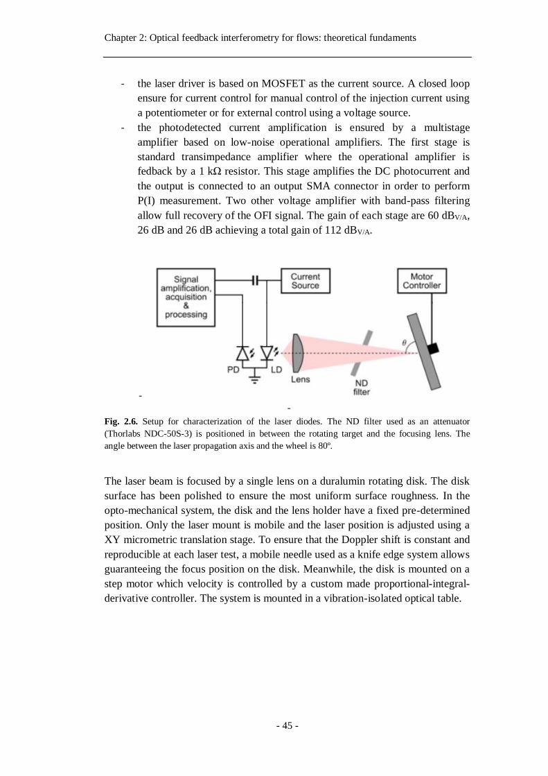
Chapter 2: Optical feedback interferometry for flows: theoretical fundaments
- 45 -
- the laser driver is based on MOSFET as the current source. A closed loop
ensure for current control for manual control of the injection current using
a potentiometer or for external control using a voltage source.
- the photodetected current amplification is ensured by a multistage
amplifier based on low-noise operational amplifiers. The first stage is
standard transimpedance amplifier where the operational amplifier is
fedback by a 1 kΩ resistor. This stage amplifies the DC photocurrent and
the output is connected to an output SMA connector in order to perform
P(I) measurement. Two other voltage amplifier with band-pass filtering
allow full recovery of the OFI signal. The gain of each stage are 60 dBV/A,
26 dB and 26 dB achieving a total gain of 112 dBV/A.
- -
Fig. 2.6. Setup for characterization of the laser diodes. The ND filter used as an attenuator
(Thorlabs NDC-50S-3) is positioned in between the rotating target and the focusing lens. The
angle between the laser propagation axis and the wheel is 80º.
The laser beam is focused by a single lens on a duralumin rotating disk. The disk
surface has been polished to ensure the most uniform surface roughness. In the
opto-mechanical system, the disk and the lens holder have a fixed pre-determined
position. Only the laser mount is mobile and the laser position is adjusted using a
XY micrometric translation stage. To ensure that the Doppler shift is constant and
reproducible at each laser test, a mobile needle used as a knife edge system allows
guaranteeing the focus position on the disk. Meanwhile, the disk is mounted on a
step motor which velocity is controlled by a custom made proportional-integral-
derivative controller. The system is mounted in a vibration-isolated optical table.
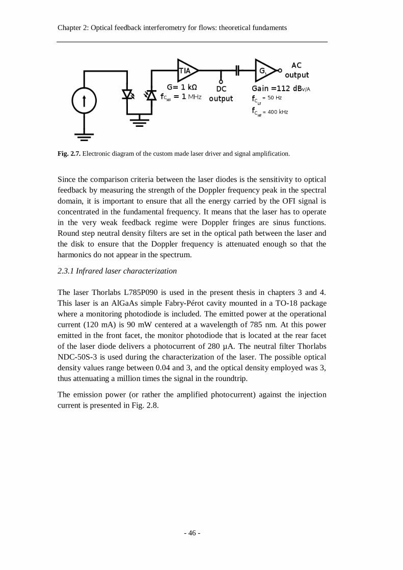
Chapter 2: Optical feedback interferometry for flows: theoretical fundaments
- 46 -
Fig. 2.7. Electronic diagram of the custom made laser driver and signal amplification.
Since the comparison criteria between the laser diodes is the sensitivity to optical
feedback by measuring the strength of the Doppler frequency peak in the spectral
domain, it is important to ensure that all the energy carried by the OFI signal is
concentrated in the fundamental frequency. It means that the laser has to operate
in the very weak feedback regime were Doppler fringes are sinus functions.
Round step neutral density filters are set in the optical path between the laser and
the disk to ensure that the Doppler frequency is attenuated enough so that the
harmonics do not appear in the spectrum.
2.3.1 Infrared laser characterization
The laser Thorlabs L785P090 is used in the present thesis in chapters 3 and 4.
This laser is an AlGaAs simple Fabry-Pérot cavity mounted in a TO-18 package
where a monitoring photodiode is included. The emitted power at the operational
current (120 mA) is 90 mW centered at a wavelength of 785 nm. At this power
emitted in the front facet, the monitor photodiode that is located at the rear facet
of the laser diode delivers a photocurrent of 280 µA. The neutral filter Thorlabs
NDC-50S-3 is used during the characterization of the laser. The possible optical
density values range between 0.04 and 3, and the optical density employed was 3,
thus attenuating a million times the signal in the roundtrip.
The emission power (or rather the amplified photocurrent) against the injection
current is presented in Fig. 2.8.
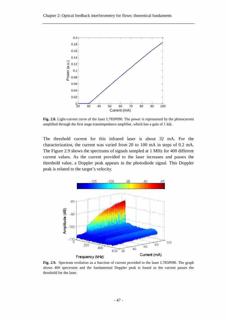
Chapter 2: Optical feedback interferometry for flows: theoretical fundaments
- 47 -
Fig. 2.8. Light-current curve of the laser L785P090. The power is represented by the photocurrent
amplified through the first stage transimpedance amplifier, which has a gain of 1 kΩ.
The threshold current for this infrared laser is about 32 mA. For the
characterization, the current was varied from 20 to 100 mA in steps of 0.2 mA.
The Figure 2.9 shows the spectrums of signals sampled at 1 MHz for 400 different
current values. As the current provided to the laser increases and passes the
threshold value, a Doppler peak appears in the photodiode signal. This Doppler
peak is related to the target’s velocity.
Fig. 2.9. Spectrum evolution as a function of current provided to the laser L785P090. The graph
shows 400 spectrums and the fundamental Doppler peak is found as the current passes the
threshold for the laser.
20 30 40 50 60 70 80 90 1000
0.02
0.04
0.06
0.08
0.1
0.12
0.14
0.16
0.18
0.2
Current (mA)
Po
we
r (a
.u.)
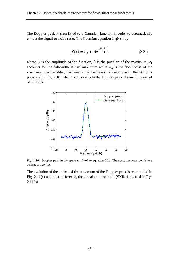
Chapter 2: Optical feedback interferometry for flows: theoretical fundaments
- 48 -
The Doppler peak is then fitted to a Gaussian function in order to automatically
extract the signal-to-noise ratio. The Gaussian equation is given by:
𝑓(𝑥) = 𝐴0 + 𝐴𝑒−
(𝑓−𝑏)2
2𝑐12 , (2.21)
where 𝐴 is the amplitude of the function, 𝑏 is the position of the maximum, 𝑐1
accounts for the full-width at half maximum while 𝐴0 is the floor noise of the
spectrum. The variable 𝑓 represents the frequency. An example of the fitting is
presented in Fig. 2.10, which corresponds to the Doppler peak obtained at current
of 120 mA.
Fig. 2.10. Doppler peak in the spectrum fitted to equation 2.21. The spectrum corresponds to a
current of 120 mA.
The evolution of the noise and the maximum of the Doppler peak is represented in
Fig. 2.11(a) and their difference, the signal-to-noise ratio (SNR) is plotted in Fig.
2.11(b).
20 30 40 50 60 70 80 90-110
-105
-100
-95
-90
-85
-80
Frequency (kHz)
Am
plit
ud
e (
dB
)
Doppler peak
Gaussian fitting
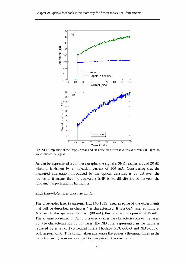
Chapter 2: Optical feedback interferometry for flows: theoretical fundaments
- 49 -
Fig. 2.11. Amplitude of the Doppler peak and the noise for different values of current (a). Signal to
noise ratio of the signal.
As can be appreciated from these graphs, the signal’s SNR reaches around 20 dB
when it is driven by an injection current of 100 mA. Considering that the
measured attenuation introduced by the optical densities is 60 dB over the
roundtrip, it means that the equivalent SNR is 80 dB distributed between the
fundamental peak and its harmonics.
2.3.2 Blue-violet laser characterization
The blue-violet laser (Panasonic DL5146-101S) used in some of the experiments
that will be described in chapter 4 is characterized. It is a GaN laser emitting at
405 nm. At the operational current (90 mA), this laser emits a power of 40 mW.
The scheme presented in Fig. 2.6 is used during the characterization of the laser.
For the characterization of this laser, the ND filter represented in the figure is
replaced by a set of two neutral filters Thorlabs NDC-50S-3 and NDC-50S-1,
both in position 6. This combination attenuates the power a thousand times in the
roundtrip and guarantees a single Doppler peak in the spectrum.
20 30 40 50 60 70 80 90 100-120
-115
-110
-105
-100
-95
-90
-85
-80
Current (mA)
Am
plit
ud
e (
dB
)
Noise
Doppler amplitude
(a)
20 30 40 50 60 70 80 90 1000
2
4
6
8
10
12
14
16
18
20
Current (mA)
Sig
na
l to
no
ise
ra
tio
(d
B)
SNR
(b)
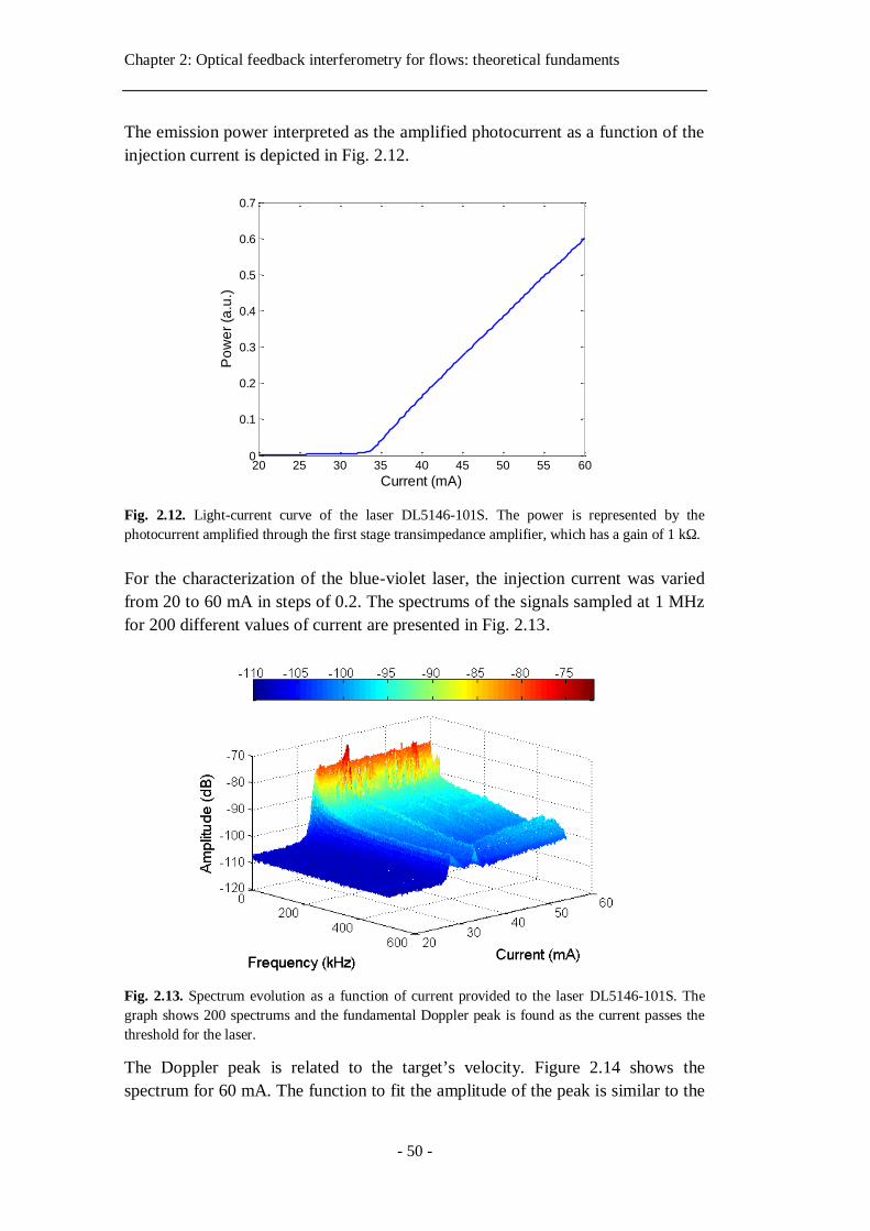
Chapter 2: Optical feedback interferometry for flows: theoretical fundaments
- 50 -
The emission power interpreted as the amplified photocurrent as a function of the
injection current is depicted in Fig. 2.12.
Fig. 2.12. Light-current curve of the laser DL5146-101S. The power is represented by the
photocurrent amplified through the first stage transimpedance amplifier, which has a gain of 1 kΩ.
For the characterization of the blue-violet laser, the injection current was varied
from 20 to 60 mA in steps of 0.2. The spectrums of the signals sampled at 1 MHz
for 200 different values of current are presented in Fig. 2.13.
Fig. 2.13. Spectrum evolution as a function of current provided to the laser DL5146-101S. The
graph shows 200 spectrums and the fundamental Doppler peak is found as the current passes the
threshold for the laser.
The Doppler peak is related to the target’s velocity. Figure 2.14 shows the
spectrum for 60 mA. The function to fit the amplitude of the peak is similar to the
20 25 30 35 40 45 50 55 600
0.1
0.2
0.3
0.4
0.5
0.6
0.7
Po
we
r (a
.u.)
Current (mA)
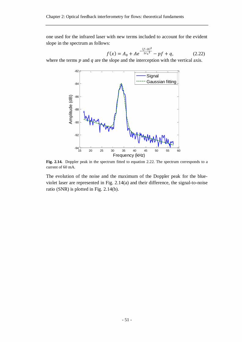
Chapter 2: Optical feedback interferometry for flows: theoretical fundaments
- 51 -
one used for the infrared laser with new terms included to account for the evident
slope in the spectrum as follows:
𝑓(𝑥) = 𝐴0 + 𝐴𝑒−
(𝑓−𝑏)2
2𝑐12 − 𝑝𝑓 + 𝑞, (2.22)
where the terms 𝑝 and 𝑞 are the slope and the interception with the vertical axis.
Fig. 2.14. Doppler peak in the spectrum fitted to equation 2.22. The spectrum corresponds to a
current of 60 mA.
The evolution of the noise and the maximum of the Doppler peak for the blue-
violet laser are represented in Fig. 2.14(a) and their difference, the signal-to-noise
ratio (SNR) is plotted in Fig. 2.14(b).
15 20 25 30 35 40 45 50 55 60-94
-92
-90
-88
-86
-84
-82
Frequency (kHz)
Am
plit
ud
e (
dB
)
Signal
Gaussian fitting
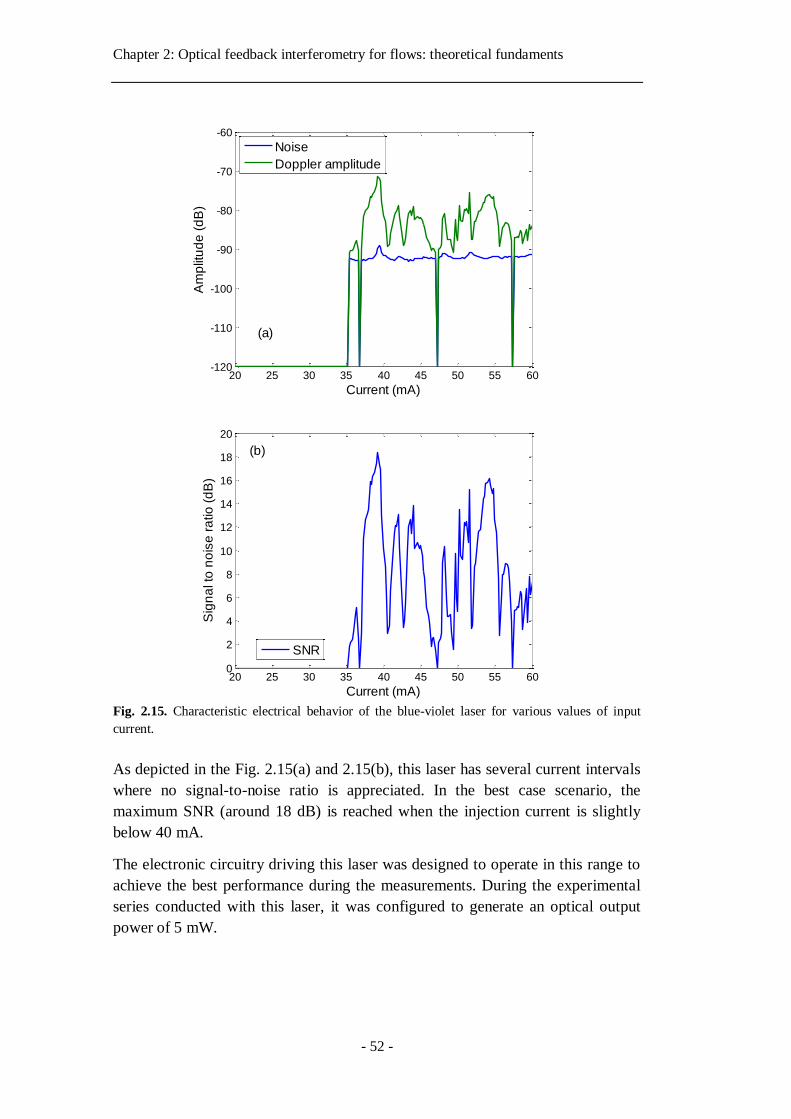
Chapter 2: Optical feedback interferometry for flows: theoretical fundaments
- 52 -
Fig. 2.15. Characteristic electrical behavior of the blue-violet laser for various values of input
current.
As depicted in the Fig. 2.15(a) and 2.15(b), this laser has several current intervals
where no signal-to-noise ratio is appreciated. In the best case scenario, the
maximum SNR (around 18 dB) is reached when the injection current is slightly
below 40 mA.
The electronic circuitry driving this laser was designed to operate in this range to
achieve the best performance during the measurements. During the experimental
series conducted with this laser, it was configured to generate an optical output
power of 5 mW.
20 25 30 35 40 45 50 55 60-120
-110
-100
-90
-80
-70
-60
Current (mA)
Am
plit
ud
e (
dB
)
Noise
Doppler amplitude
(a)
20 25 30 35 40 45 50 55 600
2
4
6
8
10
12
14
16
18
20
Current (mA)
Sig
na
l to
no
ise
ra
tio
(d
B)
SNR
(b)
Chapter 3: Optical feedback interferometry in fluid flow sensing ________________________________________________________________________
- 53 -
Chapter 3
Optical feedback interferometry in fluid flow sensing
Optical feedback interferometry (OFI) based flowmetry allows for the design of
simple, robust, self-aligned and low cost systems to measure the fluid flow. In
OFI based velocimetry (flowmetry), the OFI signal spectrum is the most usual
tool to obtain information regarding the velocity of moving objects (particles). In
the case of most solid target, the OFI signal spectrum exhibit a narrow peak at the
unique Doppler frequency induced by the target displacement. In the case of
measurement in liquids, the spectrum is strongly affected by the key elements of
the flow. The velocity distribution in the probe volume has a direct impact in the
Doppler frequency shift observed in the OFI spectrum. In addition, the spectrum
morphology is influenced by the density of scattering particles embedded in the
fluid. Depending on the particle concentration in the fluid, single scattering or
multiple scattering may occur in the sensing point causing to a significant change
in the shape of the power spectrum of the OFI sensor and thus in the methodology
for the measurement of the flow parameters.
Since the work presented in this thesis corresponds to laminar flows with
Newtonian behavior, we will focus our attention on the impact of the number of
scatterers in the sensing volume contributing to the feedback that affects the
laser’s power spectrum. We will explore the reliability of the different signal
processing methods to extract the velocity information from the OFI signals in
cases of single and multiple scattering regimes.
Chapter 3: Optical feedback interferometry in fluid flow sensing ________________________________________________________________________
- 54 -
The chapter is structured as follows. We present an analysis of the processing
methods for flow velocity measurements using an OFI sensor in the case of
multiple particles detection. A demonstration of the reliability of the signal
processing is presented for each scattering regime and two applications in the
different scattering regime are presented. First, an ex-vivo demonstration of flow
mapping using an automatic processing in the single scattering regime is
presented. Then, we present a real-time OFI system for non-steady flow
measurements in the multiple scattering regime. The chapter presents in its last
section a system for single micro-particle detection in microfluidic devices.
3.1 Reliability of optical feedback flowmetry: implications of the scattering
regime.
Under flow-controlled conditions where a laminar behavior at low Reynold
number is guaranteed, the challenge of measuring the flow rate or a local velocity
with the OFI sensing technique lies in dealing with a robust processing to extract
the quantitative velocity value. The scattering regime, because it induces various
Doppler shifts to the back-scattered waves, imposes particular power spectrum
morphologies as will be depicted lower. Thereby, different signal processing
methods have been proposed to accurately extract the Doppler frequency from the
power spectrum corresponding to the fluid velocity at the measurement volume.
In this section, the reliability of the commonly used methods for various particle
concentrations and at different flow rates is evaluated. To highlight the
performances of the signal processing approaches, velocity profile measurements
of flowing fluids in a circular microchannel by OFI for different particle
concentrations are performed.
3.1.1 Processing Methods
As described above, the particle concentration in the sensing volume of the OFI
sensor determines the power spectrum shape. In the case of very low
concentration where only one particle crosses the sensing volume at the time, the
signal spectrum exhibits a clear Doppler frequency peak. This case does not
require a very complex signal processing approach and will be developed later in
this chapter. For low particle concentrations and a small sensing volume as
compared to the channel dimension, a well-defined Doppler frequency peak
appears in the power spectrum [Rovati, 2011; Campagnolo, 2013a]. When the
dimension of the sensing volume is larger than the channel diameter, the Doppler
frequency peak becomes broader and may reach to an extent that no peak will be
observed and the spectrum exhibits a flat distribution [Riva, 1972]. As the particle
density increases, the signal spectrum is the sum of all contributions of each
particles inside the sensing volume and the spectrum shows a slow decay from
low to higher frequencies [Bonner, 1981]. Examples of this phenomenon are
depicted in Fig. 3.1 for a highly diluted solution of polystyrene spheres (0.1 % in
destilled water) and for blood flowing in a 200 μm diameter tube. The dashed
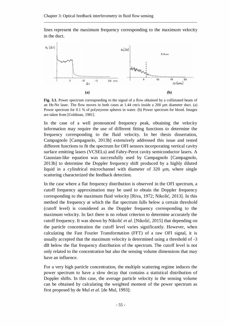
Chapter 3: Optical feedback interferometry in fluid flow sensing ________________________________________________________________________
- 55 -
lines represent the maximum frequency corresponding to the maximum velocity
in the duct.
(a) (b)
Fig. 3.1. Power spectrum corresponding to the signal of a flow obtained by a collimated beam of
an He-Ne laser. The flow moves in both cases at 1.44 cm/s inside a 200 μm diameter duct. (a)
Power spectrum for 0.1 % of polystyrene spheres in water. (b) Power spectrum for blood. Images
are taken from [Goldman, 1981].
In the case of a well pronounced frequency peak, obtaining the velocity
information may require the use of different fitting functions to determine the
frequency corresponding to the fluid velocity. In her thesis dissertation,
Campagnolo [Campagnolo, 2013b] extensively addressed this issue and tested
different functions to fit the spectrum for OFI sensors incorporating vertical cavity
surface emitting lasers (VCSELs) and Fabry-Perot cavity semiconductor lasers. A
Gaussian-like equation was successfully used by Campagnolo [Campagnolo,
2013b] to determine the Doppler frequency shift produced by a highly diluted
liquid in a cylindrical microchannel with diameter of 320 μm, where single
scattering characterized the feedback detection.
In the case where a flat frequency distribution is observed in the OFI spectrum, a
cutoff frequency approximation may be used to obtain the Doppler frequency
corresponding to the maximum fluid velocity [Riva, 1972; Nikolić, 2013]. In this
method the frequency at which the flat spectrum falls below a certain threshold
(cutoff level) is considered as the Doppler frequency corresponding to the
maximum velocity. In fact there is no robust criterion to determine accurately the
cutoff frequency. It was shown by Nikolić et al. [Nikolić, 2015] that depending on
the particle concentration the cutoff level varies significantly. However, when
calculating the Fast Fourier Transformation (FFT) of a raw OFI signal, it is
usually accepted that the maximum velocity is determined using a threshold of -3
dB below the flat frequency distribution of the spectrum. The cutoff level is not
only related to the concentration but also the sensing volume dimensions that may
have an influence.
For a very high particle concentration, the multiple scattering regime induces the
power spectrum to have a slow decay that contains a statistical distribution of
Doppler shifts. In this case, the average particle velocity in the sensing volume
can be obtained by calculating the weighted moment of the power spectrum as
first proposed by de Mul et al. [de Mul, 1993]:
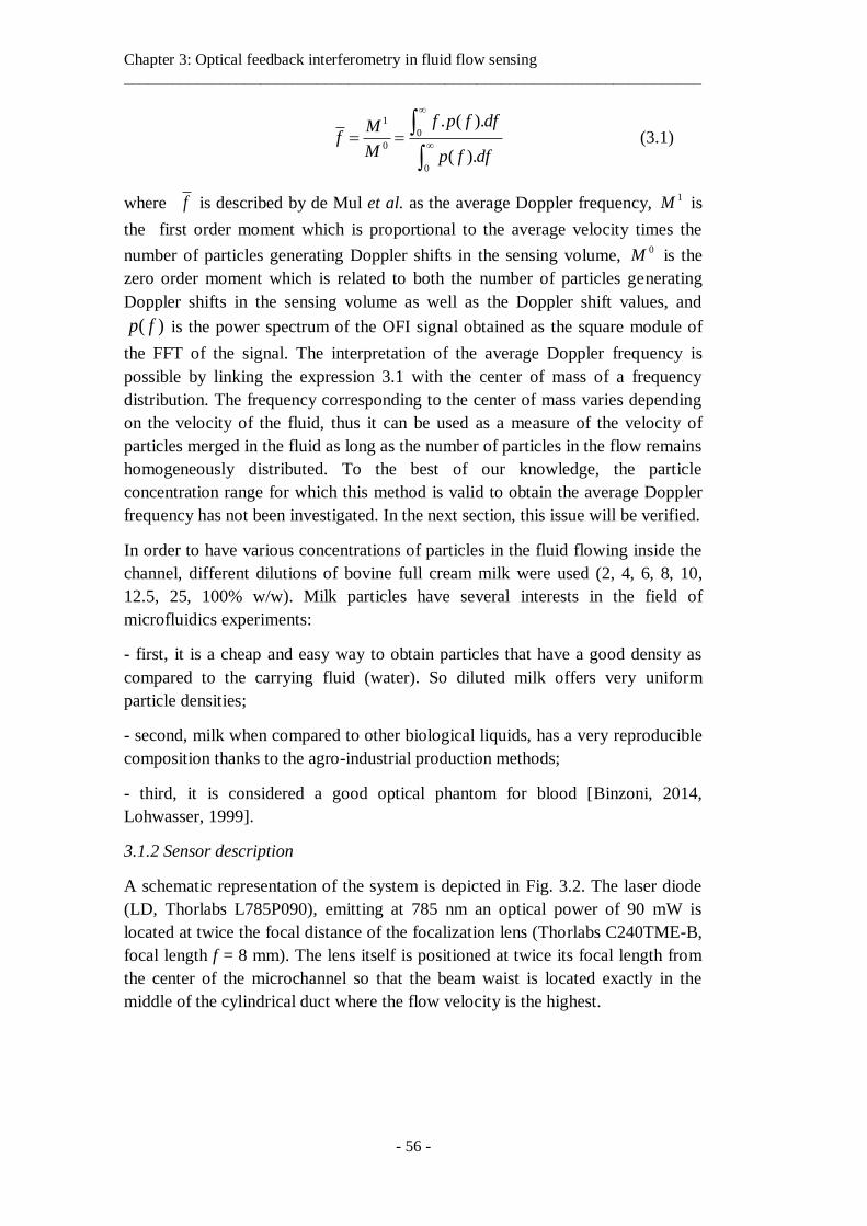
Chapter 3: Optical feedback interferometry in fluid flow sensing ________________________________________________________________________
- 56 -
1
0
0
0
. ( ).
( ).
f p f dfMf
M p f df
(3.1)
where f is described by de Mul et al. as the average Doppler frequency, 1M is
the first order moment which is proportional to the average velocity times the
number of particles generating Doppler shifts in the sensing volume, 0M is the
zero order moment which is related to both the number of particles generating
Doppler shifts in the sensing volume as well as the Doppler shift values, and
( )p f is the power spectrum of the OFI signal obtained as the square module of
the FFT of the signal. The interpretation of the average Doppler frequency is
possible by linking the expression 3.1 with the center of mass of a frequency
distribution. The frequency corresponding to the center of mass varies depending
on the velocity of the fluid, thus it can be used as a measure of the velocity of
particles merged in the fluid as long as the number of particles in the flow remains
homogeneously distributed. To the best of our knowledge, the particle
concentration range for which this method is valid to obtain the average Doppler
frequency has not been investigated. In the next section, this issue will be verified.
In order to have various concentrations of particles in the fluid flowing inside the
channel, different dilutions of bovine full cream milk were used (2, 4, 6, 8, 10,
12.5, 25, 100% w/w). Milk particles have several interests in the field of
microfluidics experiments:
- first, it is a cheap and easy way to obtain particles that have a good density as
compared to the carrying fluid (water). So diluted milk offers very uniform
particle densities;
- second, milk when compared to other biological liquids, has a very reproducible
composition thanks to the agro-industrial production methods;
- third, it is considered a good optical phantom for blood [Binzoni, 2014,
Lohwasser, 1999].
3.1.2 Sensor description
A schematic representation of the system is depicted in Fig. 3.2. The laser diode
(LD, Thorlabs L785P090), emitting at 785 nm an optical power of 90 mW is
located at twice the focal distance of the focalization lens (Thorlabs C240TME-B,
focal length f = 8 mm). The lens itself is positioned at twice its focal length from
the center of the microchannel so that the beam waist is located exactly in the
middle of the cylindrical duct where the flow velocity is the highest.
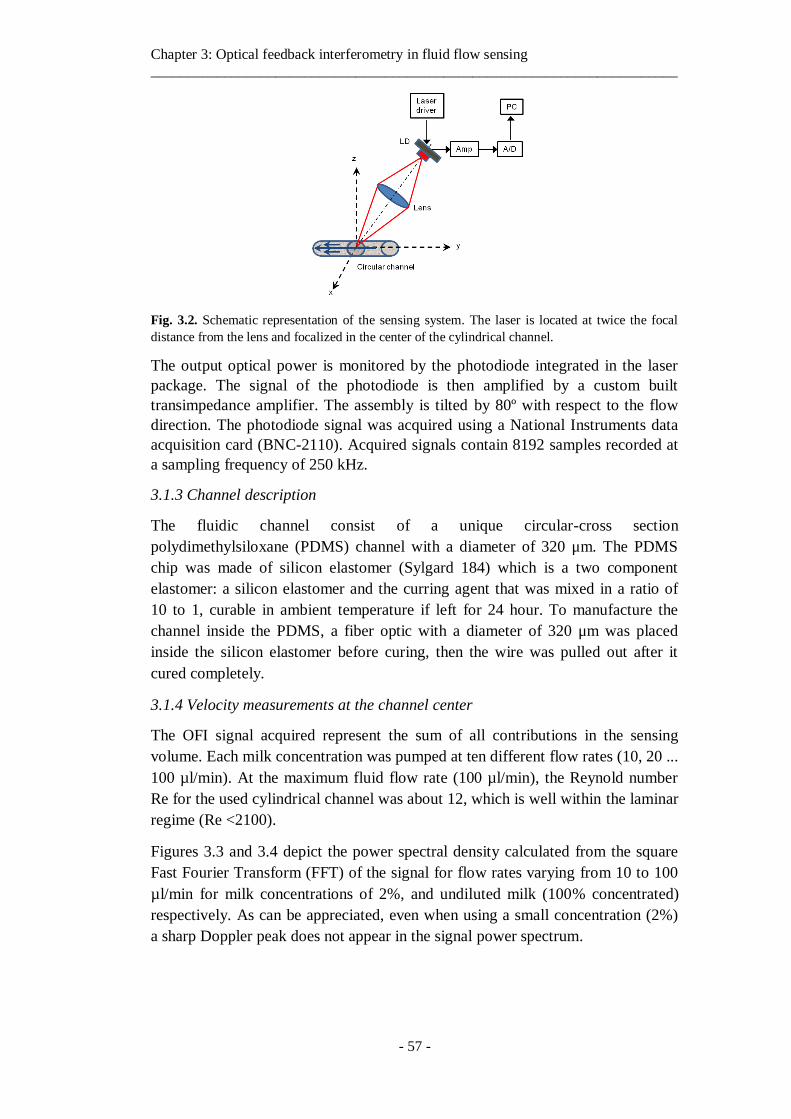
Chapter 3: Optical feedback interferometry in fluid flow sensing ________________________________________________________________________
- 57 -
Fig. 3.2. Schematic representation of the sensing system. The laser is located at twice the focal
distance from the lens and focalized in the center of the cylindrical channel.
The output optical power is monitored by the photodiode integrated in the laser
package. The signal of the photodiode is then amplified by a custom built
transimpedance amplifier. The assembly is tilted by 80º with respect to the flow
direction. The photodiode signal was acquired using a National Instruments data
acquisition card (BNC-2110). Acquired signals contain 8192 samples recorded at
a sampling frequency of 250 kHz.
3.1.3 Channel description
The fluidic channel consist of a unique circular-cross section
polydimethylsiloxane (PDMS) channel with a diameter of 320 μm. The PDMS
chip was made of silicon elastomer (Sylgard 184) which is a two component
elastomer: a silicon elastomer and the curring agent that was mixed in a ratio of
10 to 1, curable in ambient temperature if left for 24 hour. To manufacture the
channel inside the PDMS, a fiber optic with a diameter of 320 μm was placed
inside the silicon elastomer before curing, then the wire was pulled out after it
cured completely.
3.1.4 Velocity measurements at the channel center
The OFI signal acquired represent the sum of all contributions in the sensing
volume. Each milk concentration was pumped at ten different flow rates (10, 20 ...
100 µl/min). At the maximum fluid flow rate (100 µl/min), the Reynold number
Re for the used cylindrical channel was about 12, which is well within the laminar
regime (Re <2100).
Figures 3.3 and 3.4 depict the power spectral density calculated from the square
Fast Fourier Transform (FFT) of the signal for flow rates varying from 10 to 100
µl/min for milk concentrations of 2%, and undiluted milk (100% concentrated)
respectively. As can be appreciated, even when using a small concentration (2%)
a sharp Doppler peak does not appear in the signal power spectrum.
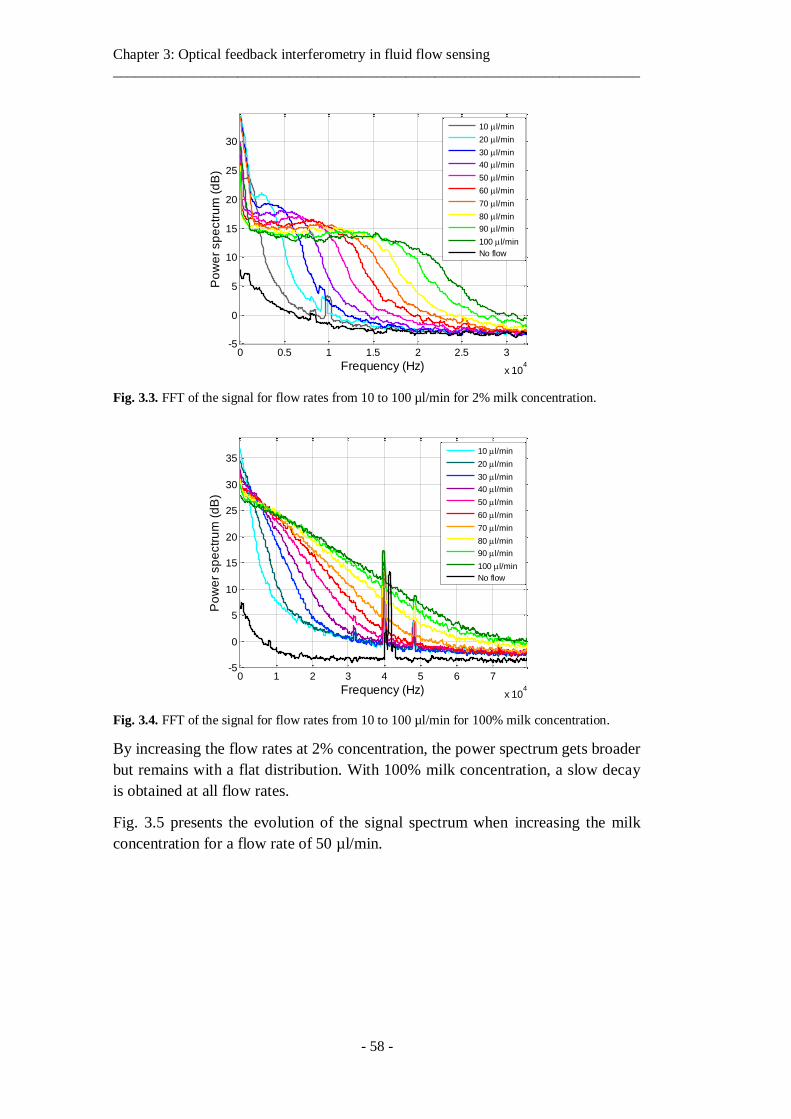
Chapter 3: Optical feedback interferometry in fluid flow sensing ________________________________________________________________________
- 58 -
Fig. 3.3. FFT of the signal for flow rates from 10 to 100 µl/min for 2% milk concentration.
Fig. 3.4. FFT of the signal for flow rates from 10 to 100 µl/min for 100% milk concentration.
By increasing the flow rates at 2% concentration, the power spectrum gets broader
but remains with a flat distribution. With 100% milk concentration, a slow decay
is obtained at all flow rates.
Fig. 3.5 presents the evolution of the signal spectrum when increasing the milk
concentration for a flow rate of 50 µl/min.
0 0.5 1 1.5 2 2.5 3
x 104
-5
0
5
10
15
20
25
30
Frequency (Hz)
Po
we
r sp
ectr
um
(d
B)
10 l/min
20 l/min
30 l/min
40 l/min
50 l/min
60 l/min
70 l/min
80 l/min
90 l/min
100 l/min
No flow
0 1 2 3 4 5 6 7
x 104
-5
0
5
10
15
20
25
30
35
Frequency (Hz)
Po
we
r sp
ectr
um
(d
B)
10 l/min
20 l/min
30 l/min
40 l/min
50 l/min
60 l/min
70 l/min
80 l/min
90 l/min
100 l/min
No flow
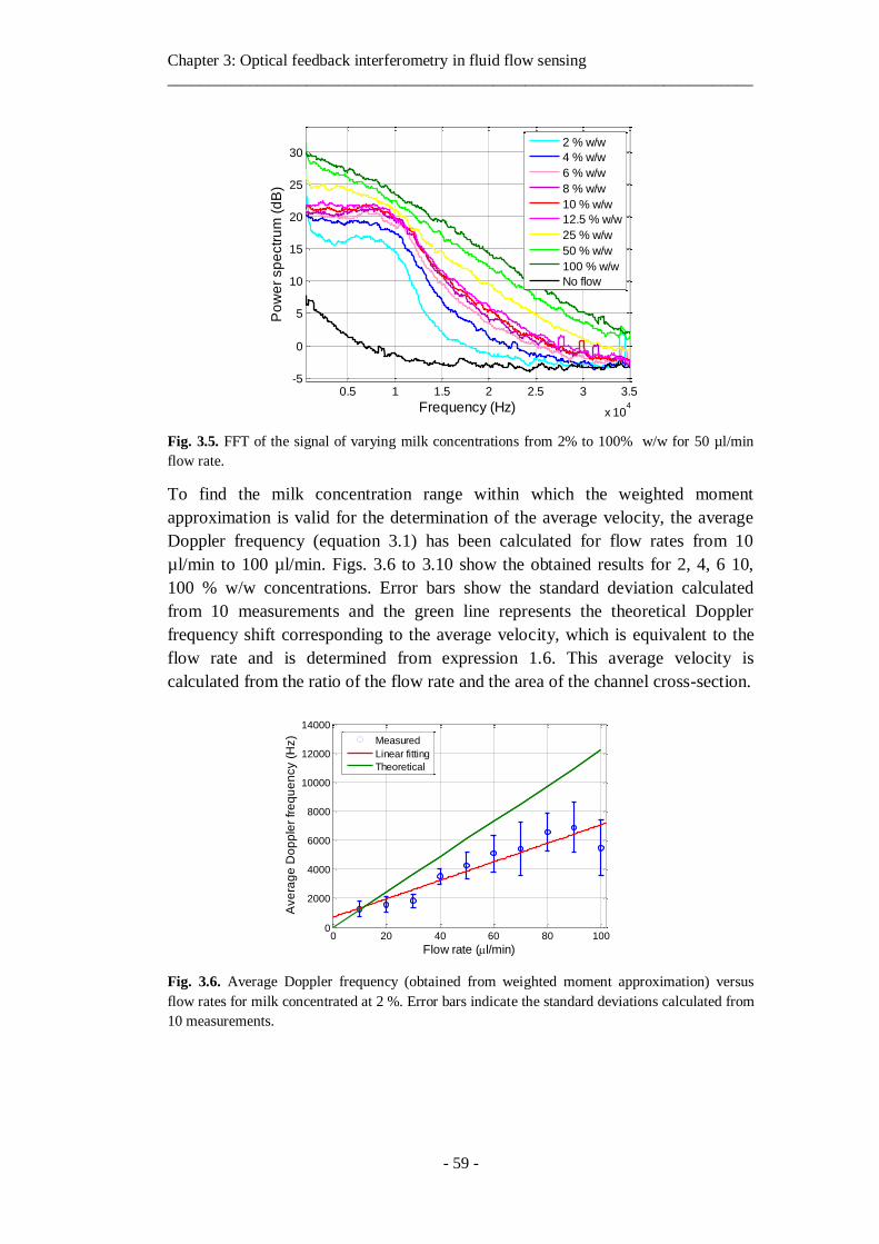
Chapter 3: Optical feedback interferometry in fluid flow sensing ________________________________________________________________________
- 59 -
Fig. 3.5. FFT of the signal of varying milk concentrations from 2% to 100% w/w for 50 µl/min
flow rate.
To find the milk concentration range within which the weighted moment
approximation is valid for the determination of the average velocity, the average
Doppler frequency (equation 3.1) has been calculated for flow rates from 10
µl/min to 100 µl/min. Figs. 3.6 to 3.10 show the obtained results for 2, 4, 6 10,
100 % w/w concentrations. Error bars show the standard deviation calculated
from 10 measurements and the green line represents the theoretical Doppler
frequency shift corresponding to the average velocity, which is equivalent to the
flow rate and is determined from expression 1.6. This average velocity is
calculated from the ratio of the flow rate and the area of the channel cross-section.
Fig. 3.6. Average Doppler frequency (obtained from weighted moment approximation) versus
flow rates for milk concentrated at 2 %. Error bars indicate the standard deviations calculated from
10 measurements.
0.5 1 1.5 2 2.5 3 3.5
x 104
-5
0
5
10
15
20
25
30
Po
we
r sp
ectr
um
(d
B)
Frequency (Hz)
2 % w/w
4 % w/w
6 % w/w
8 % w/w
10 % w/w
12.5 % w/w
25 % w/w
50 % w/w
100 % w/w
No flow
0 20 40 60 80 1000
2000
4000
6000
8000
10000
12000
14000
Flow rate (l/min)
Ave
rag
e D
op
ple
r fr
eq
ue
ncy (
Hz)
Measured
Linear fitting
Theoretical
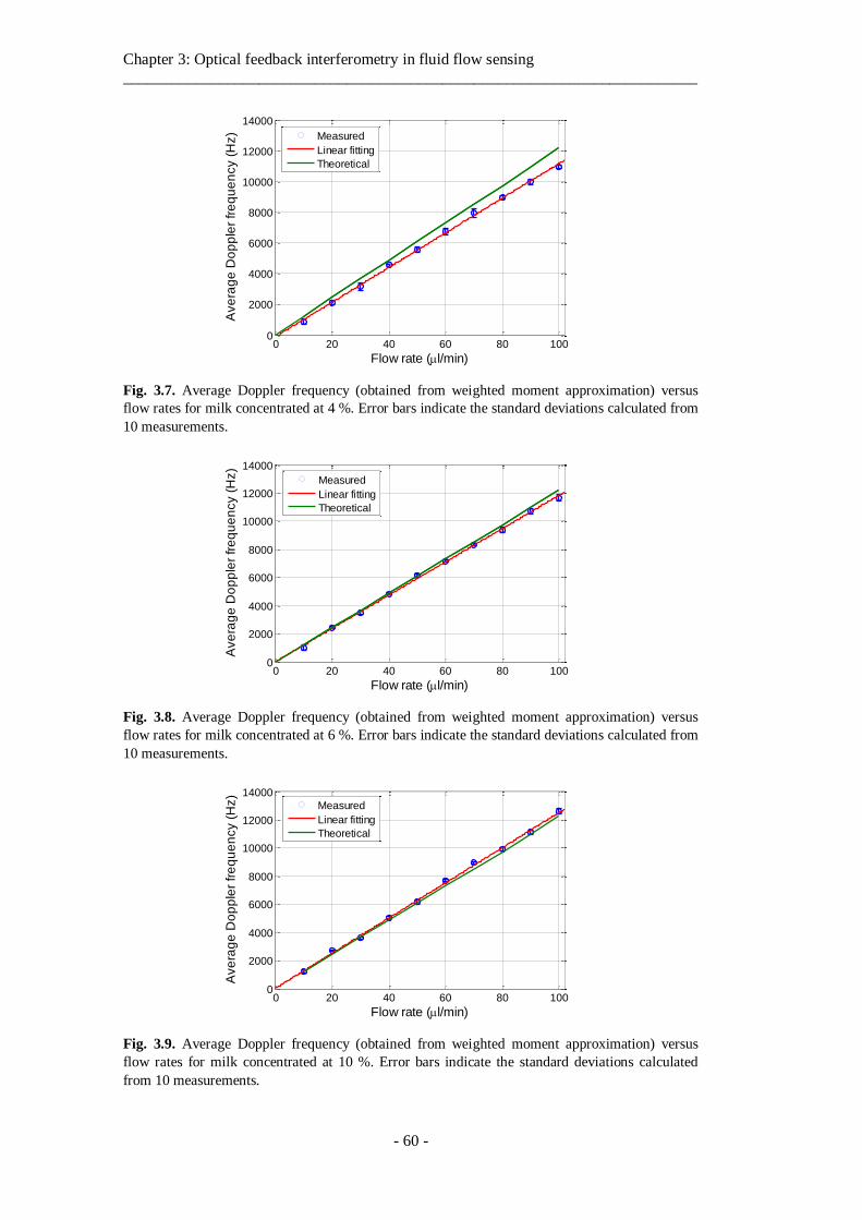
Chapter 3: Optical feedback interferometry in fluid flow sensing ________________________________________________________________________
- 60 -
Fig. 3.7. Average Doppler frequency (obtained from weighted moment approximation) versus
flow rates for milk concentrated at 4 %. Error bars indicate the standard deviations calculated from
10 measurements.
Fig. 3.8. Average Doppler frequency (obtained from weighted moment approximation) versus
flow rates for milk concentrated at 6 %. Error bars indicate the standard deviations calculated from
10 measurements.
Fig. 3.9. Average Doppler frequency (obtained from weighted moment approximation) versus
flow rates for milk concentrated at 10 %. Error bars indicate the standard deviations calculated
from 10 measurements.
0 20 40 60 80 1000
2000
4000
6000
8000
10000
12000
14000
Flow rate (l/min)
Ave
rag
e D
op
ple
r fr
eq
ue
ncy (
Hz)
Measured
Linear fitting
Theoretical
0 20 40 60 80 1000
2000
4000
6000
8000
10000
12000
14000
Flow rate (l/min)
Ave
rag
e D
op
ple
r fr
eq
ue
ncy (
Hz)
Measured
Linear fitting
Theoretical
0 20 40 60 80 1000
2000
4000
6000
8000
10000
12000
14000
Flow rate (l/min)
Ave
rag
e D
op
ple
r fr
eq
ue
ncy (
Hz)
Measured
Linear fitting
Theoretical
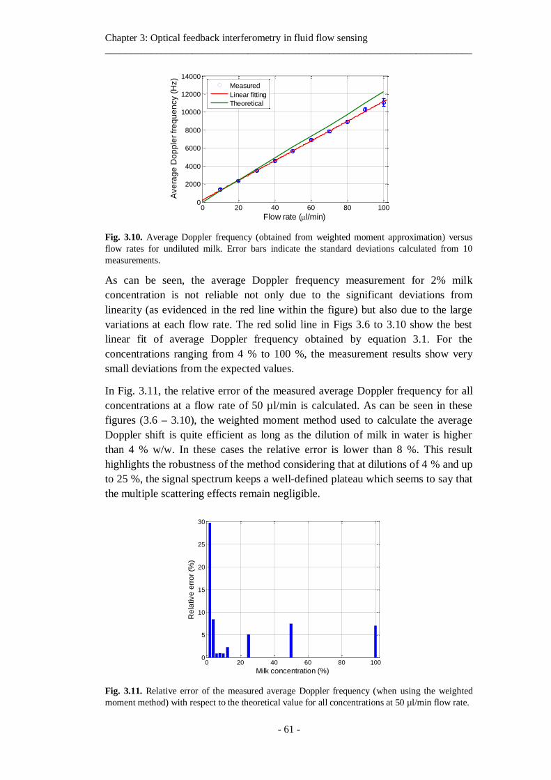
Chapter 3: Optical feedback interferometry in fluid flow sensing ________________________________________________________________________
- 61 -
Fig. 3.10. Average Doppler frequency (obtained from weighted moment approximation) versus
flow rates for undiluted milk. Error bars indicate the standard deviations calculated from 10
measurements.
As can be seen, the average Doppler frequency measurement for 2% milk
concentration is not reliable not only due to the significant deviations from
linearity (as evidenced in the red line within the figure) but also due to the large
variations at each flow rate. The red solid line in Figs 3.6 to 3.10 show the best
linear fit of average Doppler frequency obtained by equation 3.1. For the
concentrations ranging from 4 % to 100 %, the measurement results show very
small deviations from the expected values.
In Fig. 3.11, the relative error of the measured average Doppler frequency for all
concentrations at a flow rate of 50 µl/min is calculated. As can be seen in these
figures (3.6 – 3.10), the weighted moment method used to calculate the average
Doppler shift is quite efficient as long as the dilution of milk in water is higher
than 4 % w/w. In these cases the relative error is lower than 8 %. This result
highlights the robustness of the method considering that at dilutions of 4 % and up
to 25 %, the signal spectrum keeps a well-defined plateau which seems to say that
the multiple scattering effects remain negligible.
Fig. 3.11. Relative error of the measured average Doppler frequency (when using the weighted
moment method) with respect to the theoretical value for all concentrations at 50 µl/min flow rate.
0 20 40 60 80 1000
2000
4000
6000
8000
10000
12000
14000
Flow rate (l/min)
Ave
rag
e D
op
ple
r fr
eq
ue
ncy (
Hz)
Measured
Linear fitting
Theoretical
0 20 40 60 80 1000
5
10
15
20
25
30
Milk concentration (%)
Re
lative
err
or
(%)
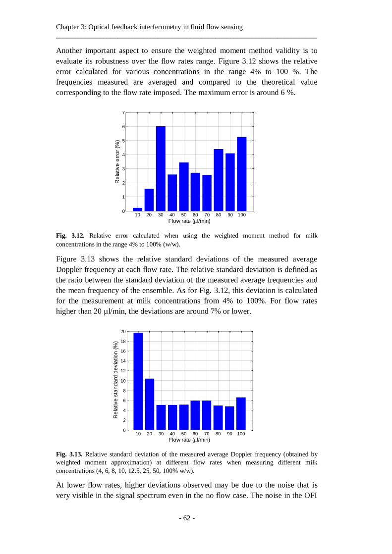
Chapter 3: Optical feedback interferometry in fluid flow sensing ________________________________________________________________________
- 62 -
Another important aspect to ensure the weighted moment method validity is to
evaluate its robustness over the flow rates range. Figure 3.12 shows the relative
error calculated for various concentrations in the range 4% to 100 %. The
frequencies measured are averaged and compared to the theoretical value
corresponding to the flow rate imposed. The maximum error is around 6 %.
Fig. 3.12. Relative error calculated when using the weighted moment method for milk
concentrations in the range 4% to 100% (w/w).
Figure 3.13 shows the relative standard deviations of the measured average
Doppler frequency at each flow rate. The relative standard deviation is defined as
the ratio between the standard deviation of the measured average frequencies and
the mean frequency of the ensemble. As for Fig. 3.12, this deviation is calculated
for the measurement at milk concentrations from 4% to 100%. For flow rates
higher than 20 µl/min, the deviations are around 7% or lower.
Fig. 3.13. Relative standard deviation of the measured average Doppler frequency (obtained by
weighted moment approximation) at different flow rates when measuring different milk
concentrations (4, 6, 8, 10, 12.5, 25, 50, 100% w/w).
At lower flow rates, higher deviations observed may be due to the noise that is
very visible in the signal spectrum even in the no flow case. The noise in the OFI
10 20 30 40 50 60 70 80 90 1000
1
2
3
4
5
6
7
Flow rate (l/min)
Re
lative
err
or
(%)
10 20 30 40 50 60 70 80 90 1000
2
4
6
8
10
12
14
16
18
20
Re
lative
sta
nd
ard
de
via
tio
n (
%)
Flow rate (l/min)
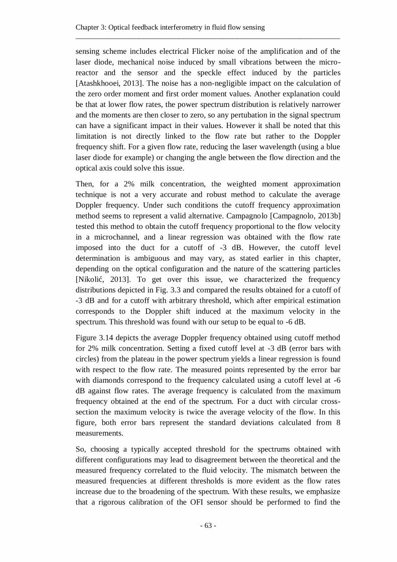
Chapter 3: Optical feedback interferometry in fluid flow sensing ________________________________________________________________________
- 63 -
sensing scheme includes electrical Flicker noise of the amplification and of the
laser diode, mechanical noise induced by small vibrations between the micro-
reactor and the sensor and the speckle effect induced by the particles
[Atashkhooei, 2013]. The noise has a non-negligible impact on the calculation of
the zero order moment and first order moment values. Another explanation could
be that at lower flow rates, the power spectrum distribution is relatively narrower
and the moments are then closer to zero, so any pertubation in the signal spectrum
can have a significant impact in their values. However it shall be noted that this
limitation is not directly linked to the flow rate but rather to the Doppler
frequency shift. For a given flow rate, reducing the laser wavelength (using a blue
laser diode for example) or changing the angle between the flow direction and the
optical axis could solve this issue.
Then, for a 2% milk concentration, the weighted moment approximation
technique is not a very accurate and robust method to calculate the average
Doppler frequency. Under such conditions the cutoff frequency approximation
method seems to represent a valid alternative. Campagnolo [Campagnolo, 2013b]
tested this method to obtain the cutoff frequency proportional to the flow velocity
in a microchannel, and a linear regression was obtained with the flow rate
imposed into the duct for a cutoff of -3 dB. However, the cutoff level
determination is ambiguous and may vary, as stated earlier in this chapter,
depending on the optical configuration and the nature of the scattering particles
[Nikolić, 2013]. To get over this issue, we characterized the frequency
distributions depicted in Fig. 3.3 and compared the results obtained for a cutoff of
-3 dB and for a cutoff with arbitrary threshold, which after empirical estimation
corresponds to the Doppler shift induced at the maximum velocity in the
spectrum. This threshold was found with our setup to be equal to -6 dB.
Figure 3.14 depicts the average Doppler frequency obtained using cutoff method
for 2% milk concentration. Setting a fixed cutoff level at -3 dB (error bars with
circles) from the plateau in the power spectrum yields a linear regression is found
with respect to the flow rate. The measured points represented by the error bar
with diamonds correspond to the frequency calculated using a cutoff level at -6
dB against flow rates. The average frequency is calculated from the maximum
frequency obtained at the end of the spectrum. For a duct with circular cross-
section the maximum velocity is twice the average velocity of the flow. In this
figure, both error bars represent the standard deviations calculated from 8
measurements.
So, choosing a typically accepted threshold for the spectrums obtained with
different configurations may lead to disagreement between the theoretical and the
measured frequency correlated to the fluid velocity. The mismatch between the
measured frequencies at different thresholds is more evident as the flow rates
increase due to the broadening of the spectrum. With these results, we emphasize
that a rigorous calibration of the OFI sensor should be performed to find the
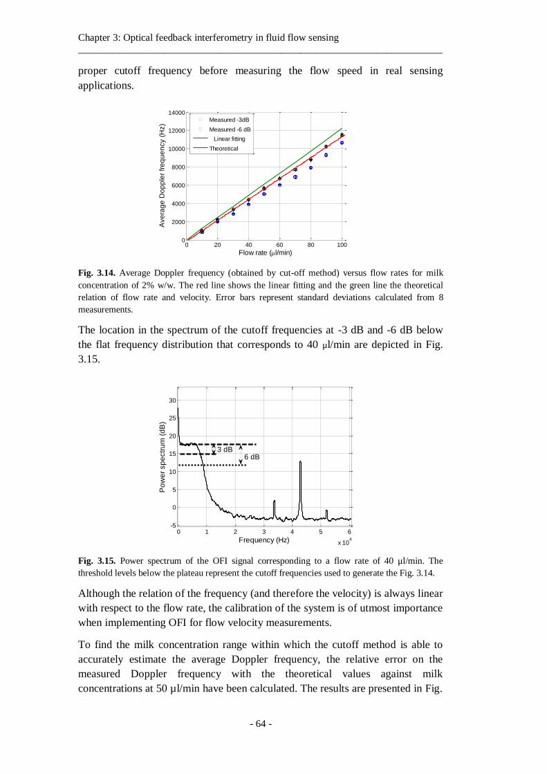
Chapter 3: Optical feedback interferometry in fluid flow sensing ________________________________________________________________________
- 64 -
proper cutoff frequency before measuring the flow speed in real sensing
applications.
Fig. 3.14. Average Doppler frequency (obtained by cut-off method) versus flow rates for milk
concentration of 2% w/w. The red line shows the linear fitting and the green line the theoretical
relation of flow rate and velocity. Error bars represent standard deviations calculated from 8
measurements.
The location in the spectrum of the cutoff frequencies at -3 dB and -6 dB below
the flat frequency distribution that corresponds to 40 μl/min are depicted in Fig.
3.15.
Fig. 3.15. Power spectrum of the OFI signal corresponding to a flow rate of 40 μl/min. The
threshold levels below the plateau represent the cutoff frequencies used to generate the Fig. 3.14.
Although the relation of the frequency (and therefore the velocity) is always linear
with respect to the flow rate, the calibration of the system is of utmost importance
when implementing OFI for flow velocity measurements.
To find the milk concentration range within which the cutoff method is able to
accurately estimate the average Doppler frequency, the relative error on the
measured Doppler frequency with the theoretical values against milk
concentrations at 50 µl/min have been calculated. The results are presented in Fig.
0 20 40 60 80 1000
2000
4000
6000
8000
10000
12000
14000
Flow rate (l/min)
Ave
rag
e D
op
ple
r fr
eq
ue
ncy (
Hz)
Measured -3dB
Measured -6 dB
Linear fitting
Theoretical
0 1 2 3 4 5 6
x 104
-5
0
5
10
15
20
25
30
Frequency (Hz)
Po
we
r sp
ectr
um
(d
B)
3 dB6 dB
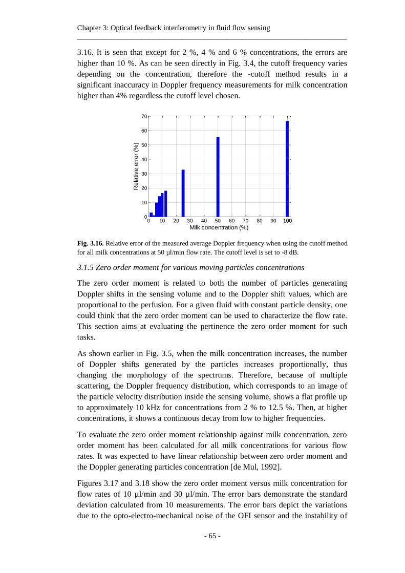
Chapter 3: Optical feedback interferometry in fluid flow sensing ________________________________________________________________________
- 65 -
3.16. It is seen that except for 2 %, 4 % and 6 % concentrations, the errors are
higher than 10 %. As can be seen directly in Fig. 3.4, the cutoff frequency varies
depending on the concentration, therefore the -cutoff method results in a
significant inaccuracy in Doppler frequency measurements for milk concentration
higher than 4% regardless the cutoff level chosen.
Fig. 3.16. Relative error of the measured average Doppler frequency when using the cutoff method
for all milk concentrations at 50 µl/min flow rate. The cutoff level is set to -8 dB.
3.1.5 Zero order moment for various moving particles concentrations
The zero order moment is related to both the number of particles generating
Doppler shifts in the sensing volume and to the Doppler shift values, which are
proportional to the perfusion. For a given fluid with constant particle density, one
could think that the zero order moment can be used to characterize the flow rate.
This section aims at evaluating the pertinence the zero order moment for such
tasks.
As shown earlier in Fig. 3.5, when the milk concentration increases, the number
of Doppler shifts generated by the particles increases proportionally, thus
changing the morphology of the spectrums. Therefore, because of multiple
scattering, the Doppler frequency distribution, which corresponds to an image of
the particle velocity distribution inside the sensing volume, shows a flat profile up
to approximately 10 kHz for concentrations from 2 % to 12.5 %. Then, at higher
concentrations, it shows a continuous decay from low to higher frequencies.
To evaluate the zero order moment relationship against milk concentration, zero
order moment has been calculated for all milk concentrations for various flow
rates. It was expected to have linear relationship between zero order moment and
the Doppler generating particles concentration [de Mul, 1992].
Figures 3.17 and 3.18 show the zero order moment versus milk concentration for
flow rates of 10 µl/min and 30 µl/min. The error bars demonstrate the standard
deviation calculated from 10 measurements. The error bars depict the variations
due to the opto-electro-mechanical noise of the OFI sensor and the instability of
0 10 20 30 40 50 60 70 80 90 1001000
10
20
30
40
50
60
70
Milk concentration (%)
Re
lative
err
or
(%)
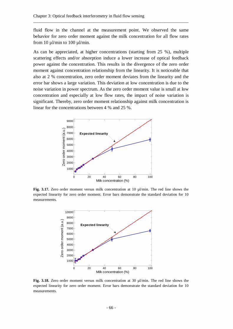
Chapter 3: Optical feedback interferometry in fluid flow sensing ________________________________________________________________________
- 66 -
fluid flow in the channel at the measurement point. We observed the same
behavior for zero order moment against the milk concentration for all flow rates
from 10 µl/min to 100 µl/min.
As can be appreciated, at higher concentrations (starting from 25 %), multiple
scattering effects and/or absorption induce a lower increase of optical feedback
power against the concentration. This results in the divergence of the zero order
moment against concentration relationship from the linearity. It is noticeable that
also at 2 % concentration, zero order moment deviates from the linearity and the
error bar shows a large variation. This deviation at low concentration is due to the
noise variation in power spectrum. As the zero order moment value is small at low
concentration and especially at low flow rates, the impact of noise variation is
significant. Thereby, zero order moment relationship against milk concentration is
linear for the concentrations between 4 % and 25 %.
Fig. 3.17. Zero order moment versus milk concentration at 10 µl/min. The red line shows the
expected linearity for zero order moment. Error bars demonstrate the standard deviation for 10
measurements.
Fig. 3.18. Zero order moment versus milk concentration at 30 µl/min. The red line shows the
expected linearity for zero order moment. Error bars demonstrate the standard deviation for 10
measurements.
0 20 40 60 80 100
1000
2000
3000
4000
5000
6000
7000
8000
9000
Milk concentration (%)
Ze
ro o
rde
r m
om
en
t (a
.u.)
Expected linearity
0 20 40 60 80 100
1000
2000
3000
4000
5000
6000
7000
8000
9000
10000
Milk concentration (%)
Ze
ro o
rde
r m
om
en
t (a
.u.)
Expected linearity
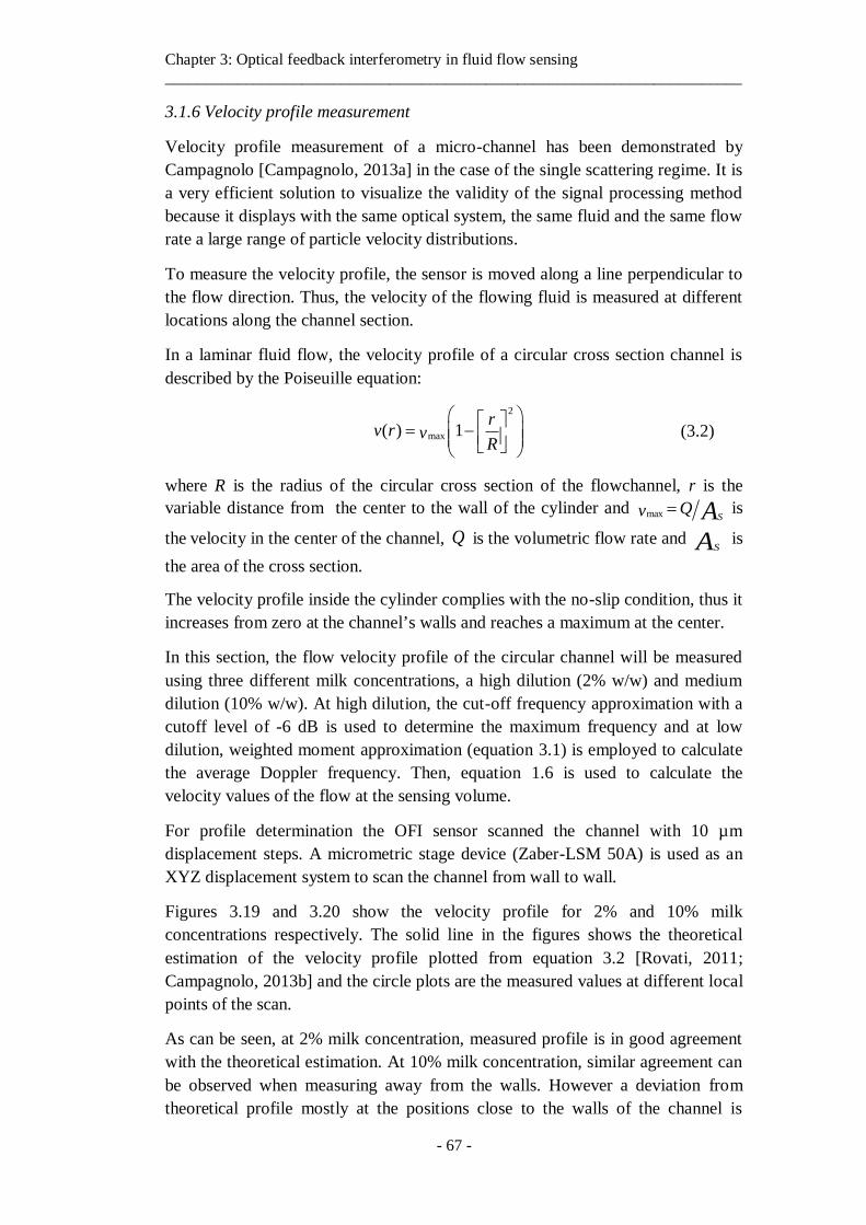
Chapter 3: Optical feedback interferometry in fluid flow sensing ________________________________________________________________________
- 67 -
3.1.6 Velocity profile measurement
Velocity profile measurement of a micro-channel has been demonstrated by
Campagnolo [Campagnolo, 2013a] in the case of the single scattering regime. It is
a very efficient solution to visualize the validity of the signal processing method
because it displays with the same optical system, the same fluid and the same flow
rate a large range of particle velocity distributions.
To measure the velocity profile, the sensor is moved along a line perpendicular to
the flow direction. Thus, the velocity of the flowing fluid is measured at different
locations along the channel section.
In a laminar fluid flow, the velocity profile of a circular cross section channel is
described by the Poiseuille equation:
2
max( ) 1r
v r vR
(3.2)
where R is the radius of the circular cross section of the flowchannel, r is the
variable distance from the center to the wall of the cylinder and max SQv A is
the velocity in the center of the channel, Q is the volumetric flow rate and SA is
the area of the cross section.
The velocity profile inside the cylinder complies with the no-slip condition, thus it
increases from zero at the channel’s walls and reaches a maximum at the center.
In this section, the flow velocity profile of the circular channel will be measured
using three different milk concentrations, a high dilution (2% w/w) and medium
dilution (10% w/w). At high dilution, the cut-off frequency approximation with a
cutoff level of -6 dB is used to determine the maximum frequency and at low
dilution, weighted moment approximation (equation 3.1) is employed to calculate
the average Doppler frequency. Then, equation 1.6 is used to calculate the
velocity values of the flow at the sensing volume.
For profile determination the OFI sensor scanned the channel with 10 µm
displacement steps. A micrometric stage device (Zaber-LSM 50A) is used as an
XYZ displacement system to scan the channel from wall to wall.
Figures 3.19 and 3.20 show the velocity profile for 2% and 10% milk
concentrations respectively. The solid line in the figures shows the theoretical
estimation of the velocity profile plotted from equation 3.2 [Rovati, 2011;
Campagnolo, 2013b] and the circle plots are the measured values at different local
points of the scan.
As can be seen, at 2% milk concentration, measured profile is in good agreement
with the theoretical estimation. At 10% milk concentration, similar agreement can
be observed when measuring away from the walls. However a deviation from
theoretical profile mostly at the positions close to the walls of the channel is
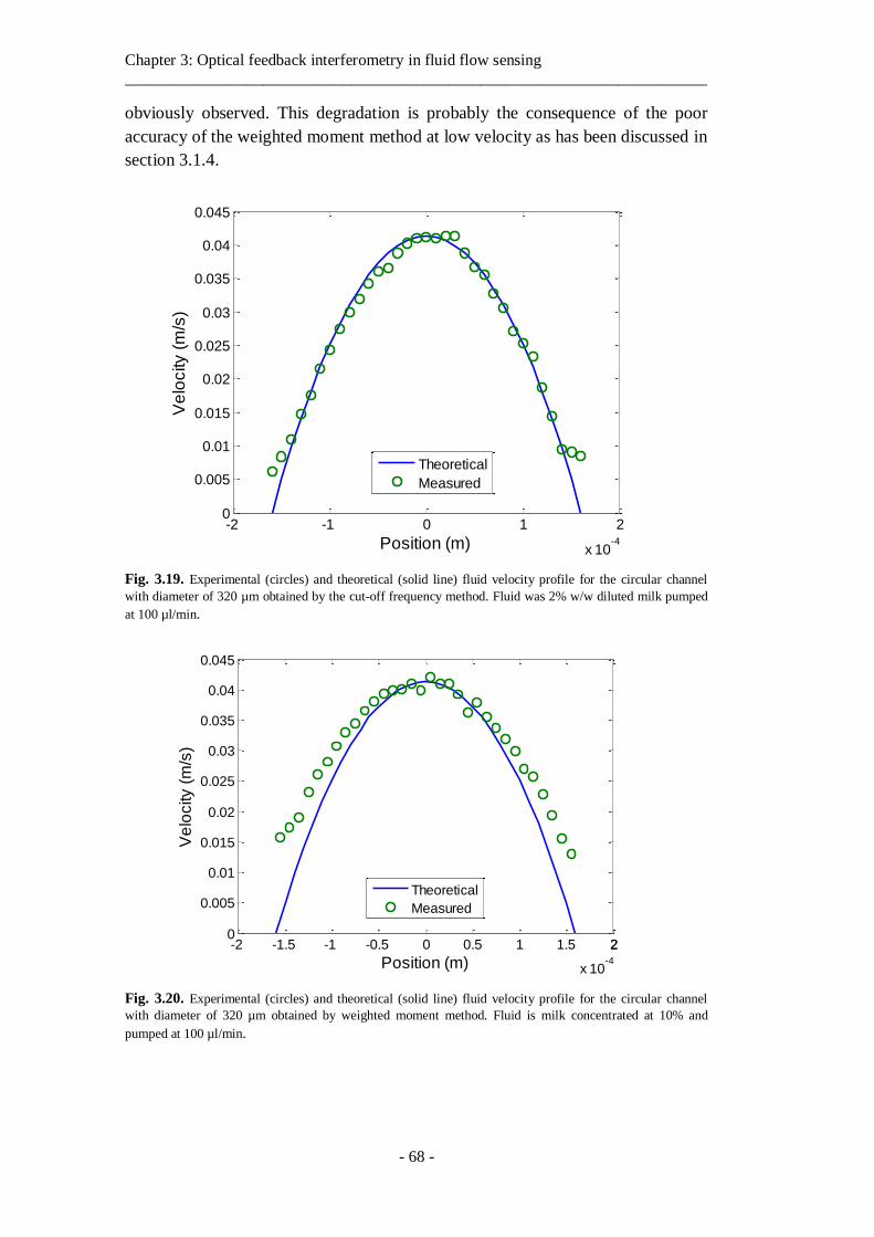
Chapter 3: Optical feedback interferometry in fluid flow sensing ________________________________________________________________________
- 68 -
obviously observed. This degradation is probably the consequence of the poor
accuracy of the weighted moment method at low velocity as has been discussed in
section 3.1.4.
Fig. 3.19. Experimental (circles) and theoretical (solid line) fluid velocity profile for the circular channel
with diameter of 320 µm obtained by the cut-off frequency method. Fluid was 2% w/w diluted milk pumped
at 100 µl/min.
Fig. 3.20. Experimental (circles) and theoretical (solid line) fluid velocity profile for the circular channel
with diameter of 320 µm obtained by weighted moment method. Fluid is milk concentrated at 10% and
pumped at 100 µl/min.
-2 -1 0 1 2
x 10-4
0
0.005
0.01
0.015
0.02
0.025
0.03
0.035
0.04
0.045
Position (m)
Ve
locity (
m/s
)
Theoretical
Measured
-2 -1.5 -1 -0.5 0 0.5 1 1.5 22
x 10-4
0
0.005
0.01
0.015
0.02
0.025
0.03
0.035
0.04
0.045
Position (m)
Ve
locity (
m/s
)
Theoretical
Measured
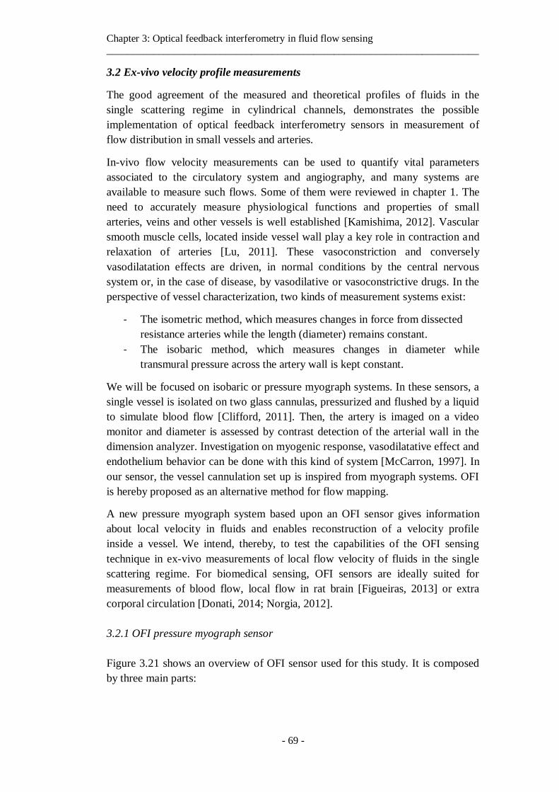
Chapter 3: Optical feedback interferometry in fluid flow sensing ________________________________________________________________________
- 69 -
3.2 Ex-vivo velocity profile measurements
The good agreement of the measured and theoretical profiles of fluids in the
single scattering regime in cylindrical channels, demonstrates the possible
implementation of optical feedback interferometry sensors in measurement of
flow distribution in small vessels and arteries.
In-vivo flow velocity measurements can be used to quantify vital parameters
associated to the circulatory system and angiography, and many systems are
available to measure such flows. Some of them were reviewed in chapter 1. The
need to accurately measure physiological functions and properties of small
arteries, veins and other vessels is well established [Kamishima, 2012]. Vascular
smooth muscle cells, located inside vessel wall play a key role in contraction and
relaxation of arteries [Lu, 2011]. These vasoconstriction and conversely
vasodilatation effects are driven, in normal conditions by the central nervous
system or, in the case of disease, by vasodilative or vasoconstrictive drugs. In the
perspective of vessel characterization, two kinds of measurement systems exist:
- The isometric method, which measures changes in force from dissected
resistance arteries while the length (diameter) remains constant.
- The isobaric method, which measures changes in diameter while
transmural pressure across the artery wall is kept constant.
We will be focused on isobaric or pressure myograph systems. In these sensors, a
single vessel is isolated on two glass cannulas, pressurized and flushed by a liquid
to simulate blood flow [Clifford, 2011]. Then, the artery is imaged on a video
monitor and diameter is assessed by contrast detection of the arterial wall in the
dimension analyzer. Investigation on myogenic response, vasodilatative effect and
endothelium behavior can be done with this kind of system [McCarron, 1997]. In
our sensor, the vessel cannulation set up is inspired from myograph systems. OFI
is hereby proposed as an alternative method for flow mapping.
A new pressure myograph system based upon an OFI sensor gives information
about local velocity in fluids and enables reconstruction of a velocity profile
inside a vessel. We intend, thereby, to test the capabilities of the OFI sensing
technique in ex-vivo measurements of local flow velocity of fluids in the single
scattering regime. For biomedical sensing, OFI sensors are ideally suited for
measurements of blood flow, local flow in rat brain [Figueiras, 2013] or extra
corporal circulation [Donati, 2014; Norgia, 2012].
3.2.1 OFI pressure myograph sensor
Figure 3.21 shows an overview of OFI sensor used for this study. It is composed
by three main parts:
Chapter 3: Optical feedback interferometry in fluid flow sensing ________________________________________________________________________
- 70 -
- XYZ displacement system. Three miniature motorized linear stages
(Zaber-LSM 50A) move the laser with a resolution of 0.1905 μm and are
controlled by a computer.
- One plano-convex optical lens (Thorlabs LA1951-B).
- A compact electronic system that realizes both laser driving and signal
amplification functions. The prototype fits on a 5x5 cm PCB.
The optical setup consists on a laser diode (Hitachi HL7851G) emitting at 785 nm
while being driven at an injection current of 50 mA. The laser is coupled to a
single lens with a focal length f = 25.4 mm and the collimated radiation is pointed
to the vessel with angle of 86°.
Fig. 3.21. OFI sensor coupled to an XYZ stage device for micrometric scanning: A) Lateral view,
B) Top view of the aorta scanning
The amplified photodiode signal is digitized by a National Instruments card (NI
USB 6251) connected via a USB interface to a computer. For each measurement
point 4096 samples are recorded at 1 MHz.
The 2D automatic scanning protocol is presented in Fig. 3.21. For each position,
10 successive series of 4096 samples are recorded and processed off-line using a
Matlab script. At the end of the recording process, each position data are stored in
a text file with 40960 samples (4096 samples x 10 records). For an aorta scanning
area of 3.75 mm2, 10 minutes are required.
The flow velocity is directly measured inside an ex vivo rat vessel with a raster
pitch of 100 μm. The size of a rat aorta is between 500 μm and 1 mm. An image
of the cannulated aorta is presented in Fig. 3.22.
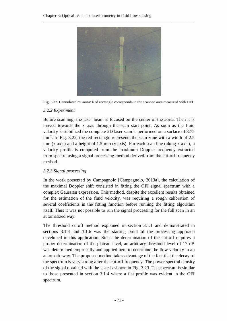
Chapter 3: Optical feedback interferometry in fluid flow sensing ________________________________________________________________________
- 71 -
Fig. 3.22. Cannulated rat aorta: Red rectangle corresponds to the scanned area measured with OFI.
3.2.2 Experiment
Before scanning, the laser beam is focused on the center of the aorta. Then it is
moved towards the x axis through the scan start point. As soon as the fluid
velocity is stabilized the complete 2D laser scan is performed on a surface of 3.75
mm2. In Fig. 3.22, the red rectangle represents the scan zone with a width of 2.5
mm (x axis) and a height of 1.5 mm (y axis). For each scan line (along x axis), a
velocity profile is computed from the maximum Doppler frequency extracted
from spectra using a signal processing method derived from the cut-off frequency
method.
3.2.3 Signal processing
In the work presented by Campagnolo [Campagnolo, 2013a], the calculation of
the maximal Doppler shift consisted in fitting the OFI signal spectrum with a
complex Gaussian expression. This method, despite the excellent results obtained
for the estimation of the fluid velocity, was requiring a rough calibration of
several coefficients in the fitting function before running the fitting algorithm
itself. Thus it was not possible to run the signal processing for the full scan in an
automatized way.
The threshold cutoff method explained in section 3.1.1 and demonstrated in
sections 3.1.4 and 3.1.6 was the starting point of the processing approach
developed in this application. Since the determination of the cut-off requires a
proper determination of the plateau level, an arbitrary threshold level of 17 dB
was determined empirically and applied here to determine the flow velocity in an
automatic way. The proposed method takes advantage of the fact that the decay of
the spectrum is very strong after the cut-off frequency. The power spectral density
of the signal obtained with the laser is shown in Fig. 3.23. The spectrum is similar
to those presented in section 3.1.4 where a flat profile was evident in the OFI
spectrum.
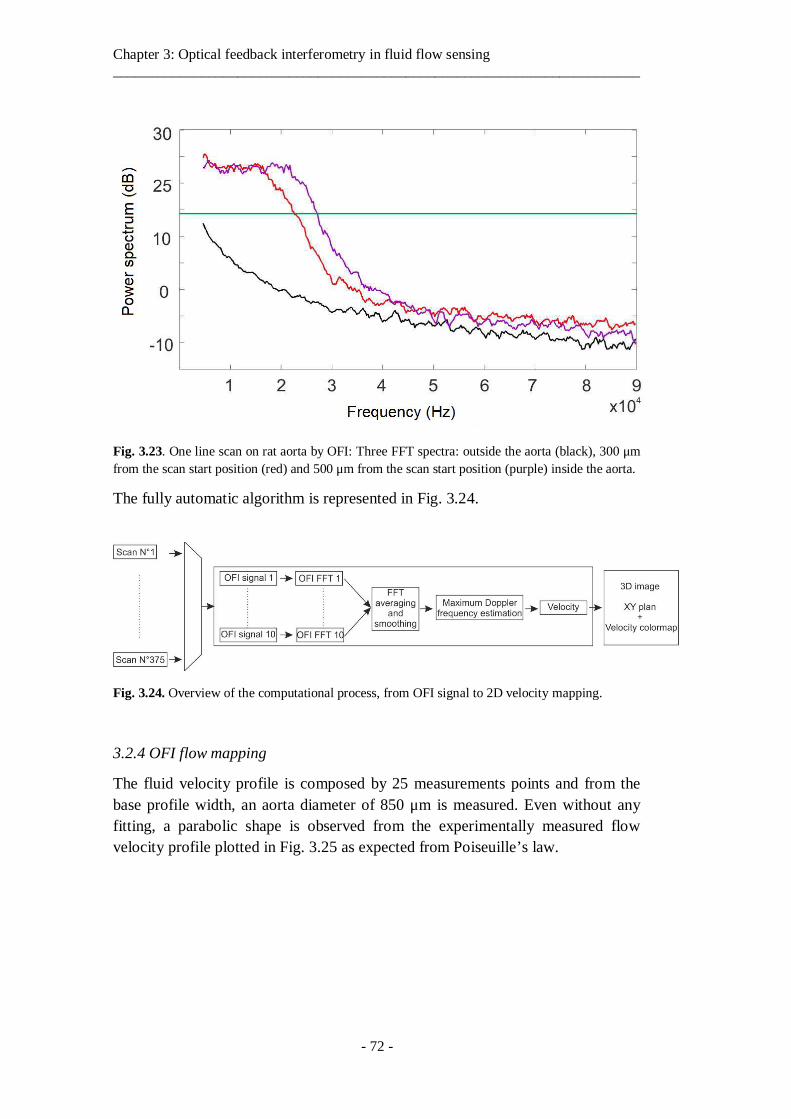
Chapter 3: Optical feedback interferometry in fluid flow sensing ________________________________________________________________________
- 72 -
Fig. 3.23. One line scan on rat aorta by OFI: Three FFT spectra: outside the aorta (black), 300 μm
from the scan start position (red) and 500 μm from the scan start position (purple) inside the aorta.
The fully automatic algorithm is represented in Fig. 3.24.
Fig. 3.24. Overview of the computational process, from OFI signal to 2D velocity mapping.
3.2.4 OFI flow mapping
The fluid velocity profile is composed by 25 measurements points and from the
base profile width, an aorta diameter of 850 μm is measured. Even without any
fitting, a parabolic shape is observed from the experimentally measured flow
velocity profile plotted in Fig. 3.25 as expected from Poiseuille’s law.
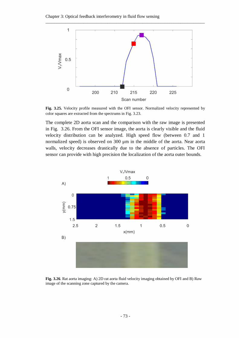
Chapter 3: Optical feedback interferometry in fluid flow sensing ________________________________________________________________________
- 73 -
Fig. 3.25. Velocity profile measured with the OFI sensor. Normalized velocity represented by
color squares are extracted from the spectrums in Fig. 3.23.
The complete 2D aorta scan and the comparison with the raw image is presented
in Fig. 3.26. From the OFI sensor image, the aorta is clearly visible and the fluid
velocity distribution can be analyzed. High speed flow (between 0.7 and 1
normalized speed) is observed on 300 μm in the middle of the aorta. Near aorta
walls, velocity decreases drastically due to the absence of particles. The OFI
sensor can provide with high precision the localization of the aorta outer bounds.
Fig. 3.26. Rat aorta imaging: A) 2D rat aorta fluid velocity imaging obtained by OFI and B) Raw
image of the scanning zone captured by the camera.
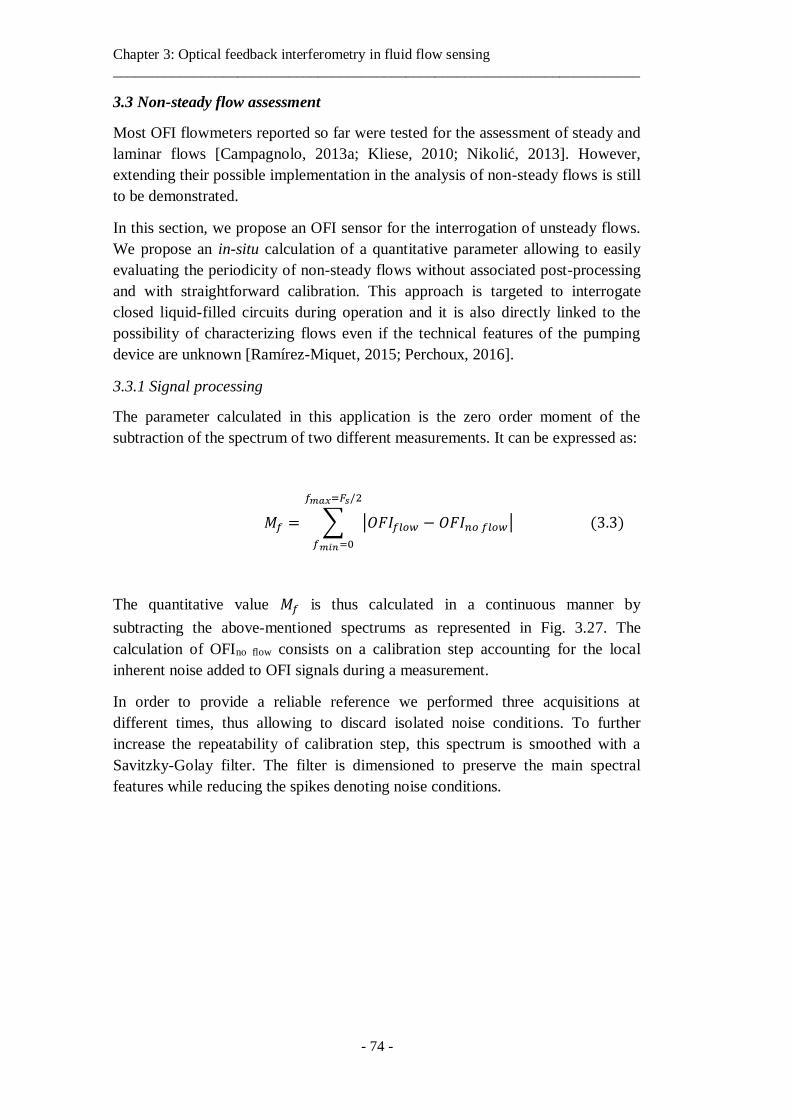
Chapter 3: Optical feedback interferometry in fluid flow sensing ________________________________________________________________________
- 74 -
3.3 Non-steady flow assessment
Most OFI flowmeters reported so far were tested for the assessment of steady and
laminar flows [Campagnolo, 2013a; Kliese, 2010; Nikolić, 2013]. However,
extending their possible implementation in the analysis of non-steady flows is still
to be demonstrated.
In this section, we propose an OFI sensor for the interrogation of unsteady flows.
We propose an in-situ calculation of a quantitative parameter allowing to easily
evaluating the periodicity of non-steady flows without associated post-processing
and with straightforward calibration. This approach is targeted to interrogate
closed liquid-filled circuits during operation and it is also directly linked to the
possibility of characterizing flows even if the technical features of the pumping
device are unknown [Ramírez-Miquet, 2015; Perchoux, 2016].
3.3.1 Signal processing
The parameter calculated in this application is the zero order moment of the
subtraction of the spectrum of two different measurements. It can be expressed as:
𝑀𝑓 = ∑ |𝑂𝐹𝐼𝑓𝑙𝑜𝑤 − 𝑂𝐹𝐼𝑛𝑜 𝑓𝑙𝑜𝑤|
𝑓𝑚𝑎𝑥=𝐹𝑠/2
𝑓𝑚𝑖𝑛=0
(3.3)
The quantitative value 𝑀𝑓 is thus calculated in a continuous manner by
subtracting the above-mentioned spectrums as represented in Fig. 3.27. The
calculation of OFIno flow consists on a calibration step accounting for the local
inherent noise added to OFI signals during a measurement.
In order to provide a reliable reference we performed three acquisitions at
different times, thus allowing to discard isolated noise conditions. To further
increase the repeatability of calibration step, this spectrum is smoothed with a
Savitzky-Golay filter. The filter is dimensioned to preserve the main spectral
features while reducing the spikes denoting noise conditions.
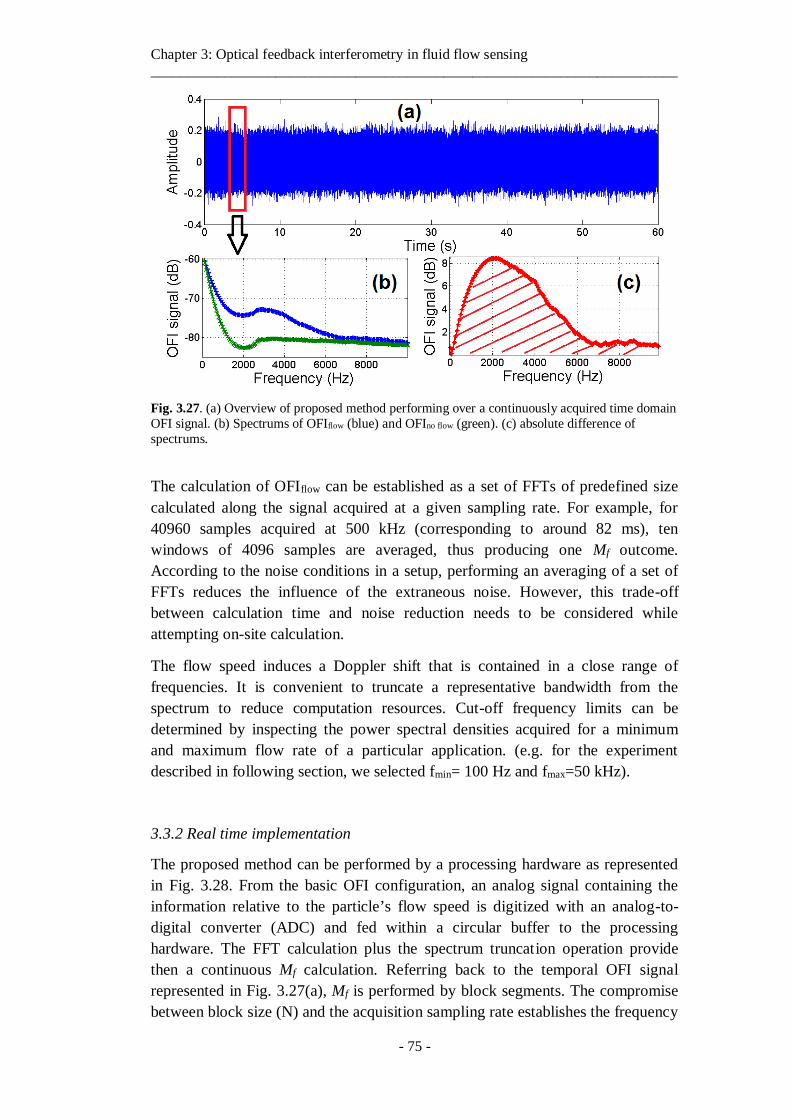
Chapter 3: Optical feedback interferometry in fluid flow sensing ________________________________________________________________________
- 75 -
Fig. 3.27. (a) Overview of proposed method performing over a continuously acquired time domain
OFI signal. (b) Spectrums of OFIflow (blue) and OFIno flow (green). (c) absolute difference of
spectrums.
The calculation of OFIflow can be established as a set of FFTs of predefined size
calculated along the signal acquired at a given sampling rate. For example, for
40960 samples acquired at 500 kHz (corresponding to around 82 ms), ten
windows of 4096 samples are averaged, thus producing one Mf outcome.
According to the noise conditions in a setup, performing an averaging of a set of
FFTs reduces the influence of the extraneous noise. However, this trade-off
between calculation time and noise reduction needs to be considered while
attempting on-site calculation.
The flow speed induces a Doppler shift that is contained in a close range of
frequencies. It is convenient to truncate a representative bandwidth from the
spectrum to reduce computation resources. Cut-off frequency limits can be
determined by inspecting the power spectral densities acquired for a minimum
and maximum flow rate of a particular application. (e.g. for the experiment
described in following section, we selected fmin= 100 Hz and fmax=50 kHz).
3.3.2 Real time implementation
The proposed method can be performed by a processing hardware as represented
in Fig. 3.28. From the basic OFI configuration, an analog signal containing the
information relative to the particle’s flow speed is digitized with an analog-to-
digital converter (ADC) and fed within a circular buffer to the processing
hardware. The FFT calculation plus the spectrum truncation operation provide
then a continuous Mf calculation. Referring back to the temporal OFI signal
represented in Fig. 3.27(a), Mf is performed by block segments. The compromise
between block size (N) and the acquisition sampling rate establishes the frequency
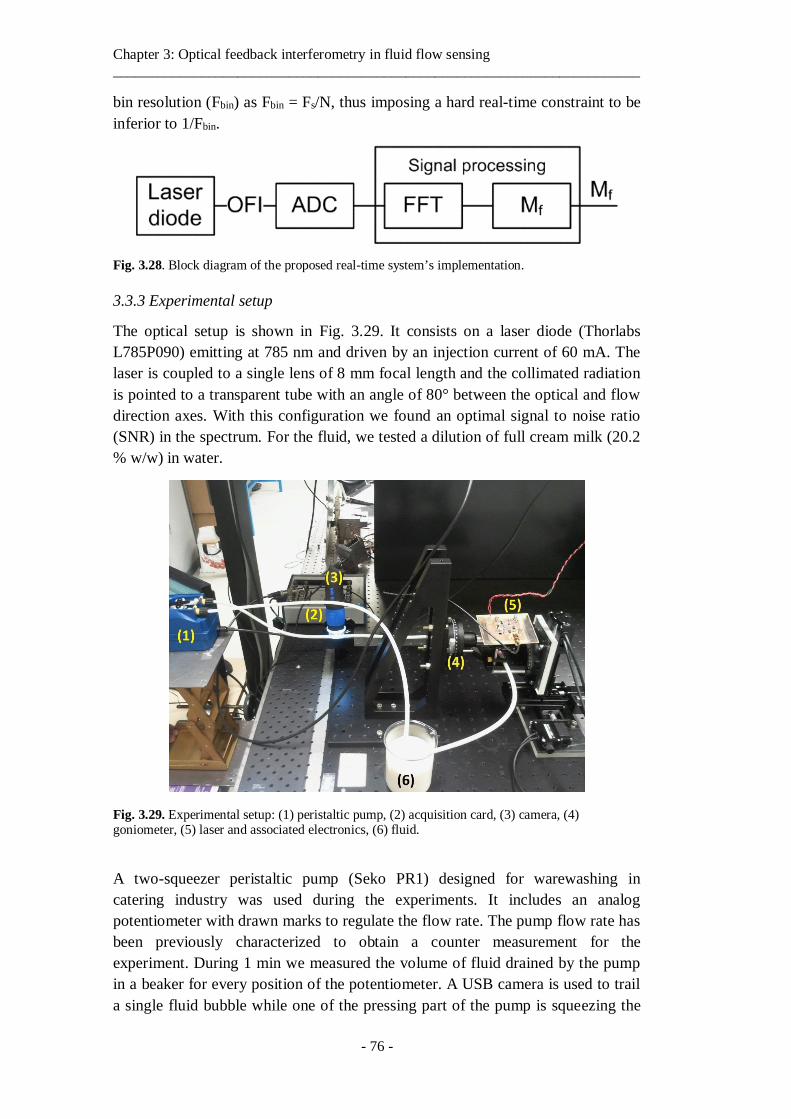
Chapter 3: Optical feedback interferometry in fluid flow sensing ________________________________________________________________________
- 76 -
bin resolution (Fbin) as Fbin = Fs/N, thus imposing a hard real-time constraint to be
inferior to 1/Fbin.
Fig. 3.28. Block diagram of the proposed real-time system’s implementation.
3.3.3 Experimental setup
The optical setup is shown in Fig. 3.29. It consists on a laser diode (Thorlabs
L785P090) emitting at 785 nm and driven by an injection current of 60 mA. The
laser is coupled to a single lens of 8 mm focal length and the collimated radiation
is pointed to a transparent tube with an angle of 80° between the optical and flow
direction axes. With this configuration we found an optimal signal to noise ratio
(SNR) in the spectrum. For the fluid, we tested a dilution of full cream milk (20.2
% w/w) in water.
Fig. 3.29. Experimental setup: (1) peristaltic pump, (2) acquisition card, (3) camera, (4) goniometer, (5) laser and associated electronics, (6) fluid.
A two-squeezer peristaltic pump (Seko PR1) designed for warewashing in
catering industry was used during the experiments. It includes an analog
potentiometer with drawn marks to regulate the flow rate. The pump flow rate has
been previously characterized to obtain a counter measurement for the
experiment. During 1 min we measured the volume of fluid drained by the pump
in a beaker for every position of the potentiometer. A USB camera is used to trail
a single fluid bubble while one of the pressing part of the pump is squeezing the
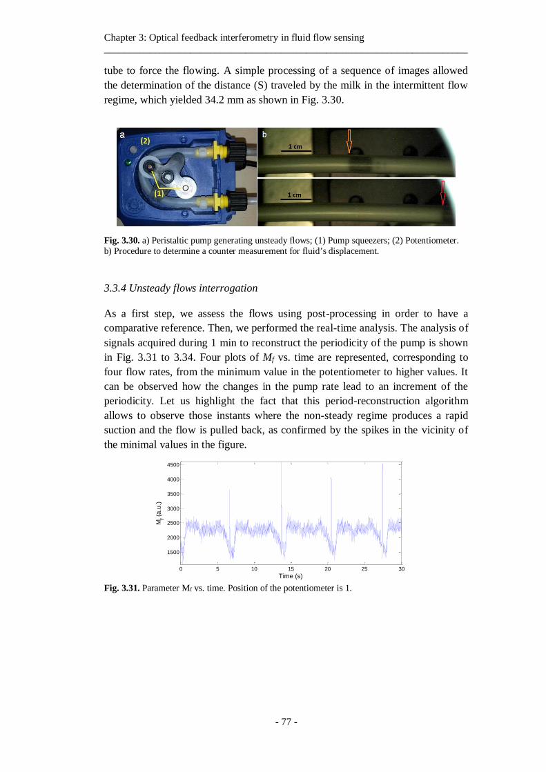
Chapter 3: Optical feedback interferometry in fluid flow sensing ________________________________________________________________________
- 77 -
tube to force the flowing. A simple processing of a sequence of images allowed
the determination of the distance (S) traveled by the milk in the intermittent flow
regime, which yielded 34.2 mm as shown in Fig. 3.30.
Fig. 3.30. a) Peristaltic pump generating unsteady flows; (1) Pump squeezers; (2) Potentiometer.
b) Procedure to determine a counter measurement for fluid’s displacement.
3.3.4 Unsteady flows interrogation
As a first step, we assess the flows using post-processing in order to have a
comparative reference. Then, we performed the real-time analysis. The analysis of
signals acquired during 1 min to reconstruct the periodicity of the pump is shown
in Fig. 3.31 to 3.34. Four plots of Mf vs. time are represented, corresponding to
four flow rates, from the minimum value in the potentiometer to higher values. It
can be observed how the changes in the pump rate lead to an increment of the
periodicity. Let us highlight the fact that this period-reconstruction algorithm
allows to observe those instants where the non-steady regime produces a rapid
suction and the flow is pulled back, as confirmed by the spikes in the vicinity of
the minimal values in the figure.
Fig. 3.31. Parameter Mf vs. time. Position of the potentiometer is 1.
0 5 10 15 20 25 30
1500
2000
2500
3000
3500
4000
4500
Mf (
a.u
.)
Time (s)
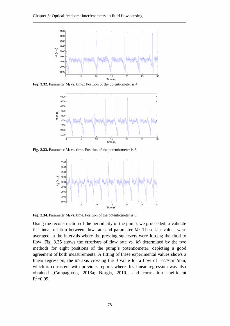
Chapter 3: Optical feedback interferometry in fluid flow sensing ________________________________________________________________________
- 78 -
Fig. 3.32. Parameter Mf vs. time.: Position of the potentiometer is 4.
Fig. 3.33. Parameter Mf vs. time. Position of the potentiometer is 6.
Fig. 3.34. Parameter Mf vs. time. Position of the potentiometer is 8.
Using the reconstruction of the periodicity of the pump, we proceeded to validate
the linear relation between flow rate and parameter Mf. These last values were
averaged in the intervals where the pressing squeezers were forcing the fluid to
flow. Fig. 3.35 shows the errorbars of flow rate vs. Mf determined by the two
methods for eight positions of the pump’s potentiometer, depicting a good
agreement of both measurements. A fitting of these experimental values shows a
linear regression, the Mf axis crossing the 0 value for a flow of -7.76 ml/min,
which is consistent with previous reports where this linear regression was also
obtained [Campagnolo, 2013a; Norgia, 2010], and correlation coefficient
R2=0.99.
0 5 10 15 20 25 30
1500
2000
2500
3000
3500
4000
4500
5000
5500
Mf (
a.u
.)
Time (s)
0 5 10 15 20 25 30
1500
2000
2500
3000
3500
4000
4500
5000
5500
Mf (
a.u
.)
Time (s)
0 5 10 15 20 25 30
1500
2000
2500
3000
3500
4000
4500
5000
5500
Mf (
a.u
.)
Time (s)
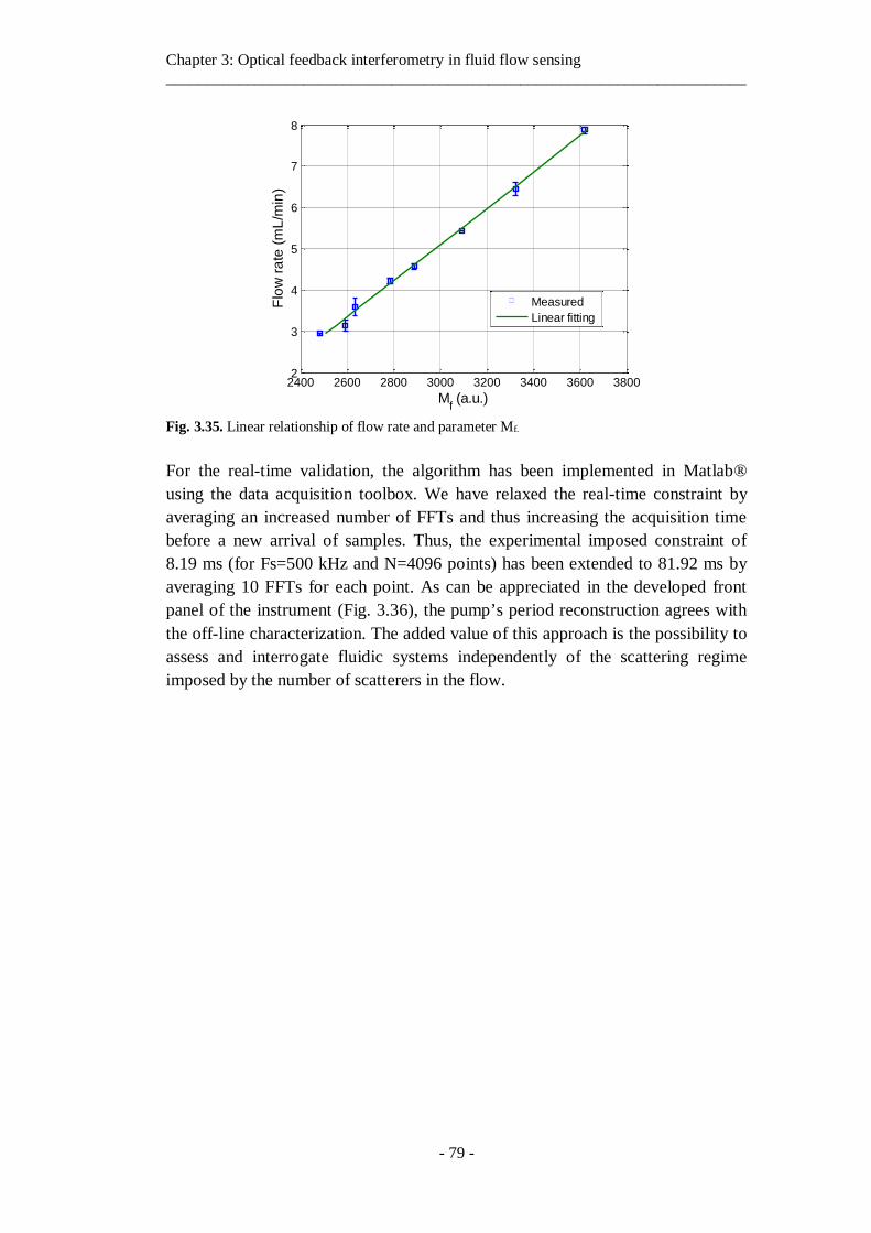
Chapter 3: Optical feedback interferometry in fluid flow sensing ________________________________________________________________________
- 79 -
Fig. 3.35. Linear relationship of flow rate and parameter Mf.
For the real-time validation, the algorithm has been implemented in Matlab®
using the data acquisition toolbox. We have relaxed the real-time constraint by
averaging an increased number of FFTs and thus increasing the acquisition time
before a new arrival of samples. Thus, the experimental imposed constraint of
8.19 ms (for Fs=500 kHz and N=4096 points) has been extended to 81.92 ms by
averaging 10 FFTs for each point. As can be appreciated in the developed front
panel of the instrument (Fig. 3.36), the pump’s period reconstruction agrees with
the off-line characterization. The added value of this approach is the possibility to
assess and interrogate fluidic systems independently of the scattering regime
imposed by the number of scatterers in the flow.
2400 2600 2800 3000 3200 3400 3600 38002
3
4
5
6
7
8
Mf (a.u.)
Flo
w r
ate
(m
L/m
in)
Measured
Linear fitting
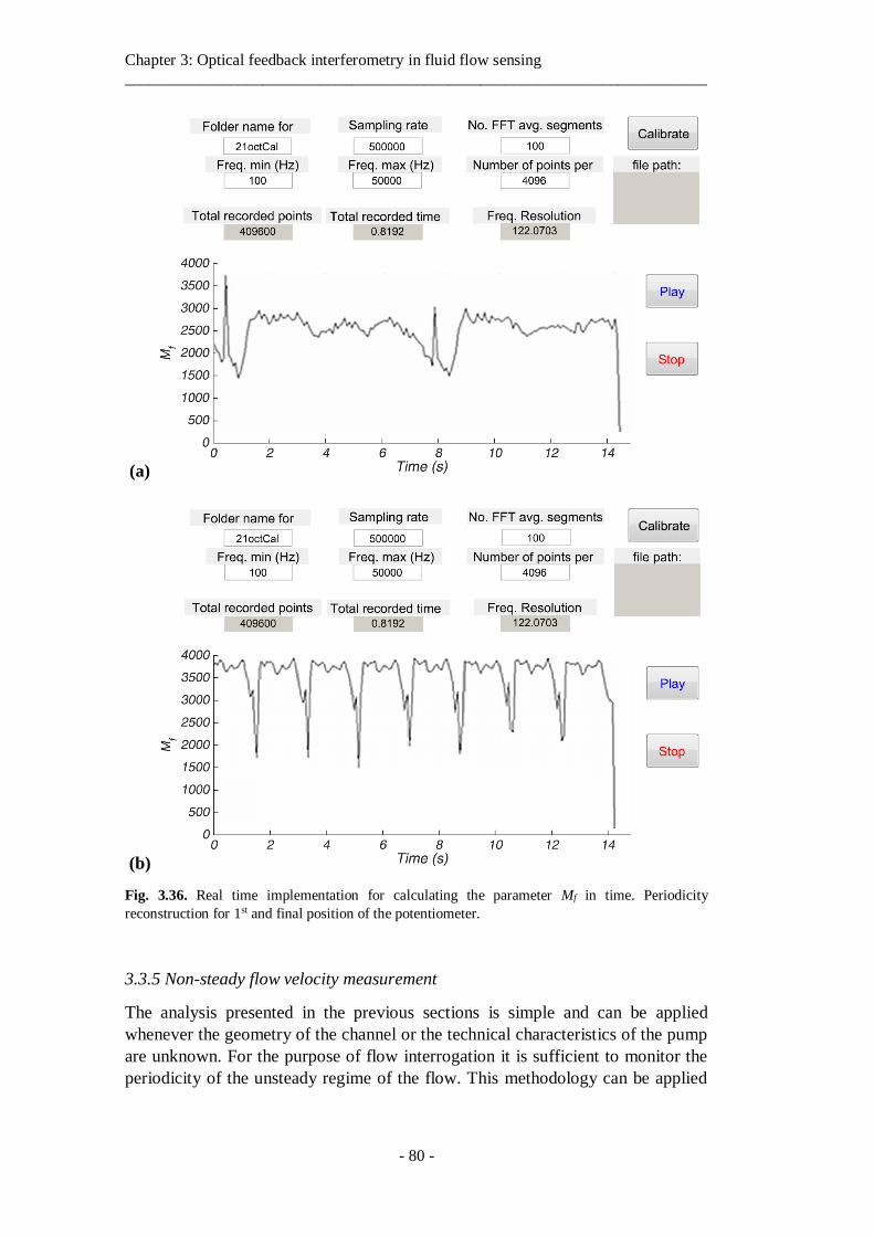
Chapter 3: Optical feedback interferometry in fluid flow sensing ________________________________________________________________________
- 80 -
(a)
(b)
Fig. 3.36. Real time implementation for calculating the parameter Mf in time. Periodicity
reconstruction for 1st and final position of the potentiometer.
3.3.5 Non-steady flow velocity measurement
The analysis presented in the previous sections is simple and can be applied
whenever the geometry of the channel or the technical characteristics of the pump
are unknown. For the purpose of flow interrogation it is sufficient to monitor the
periodicity of the unsteady regime of the flow. This methodology can be applied
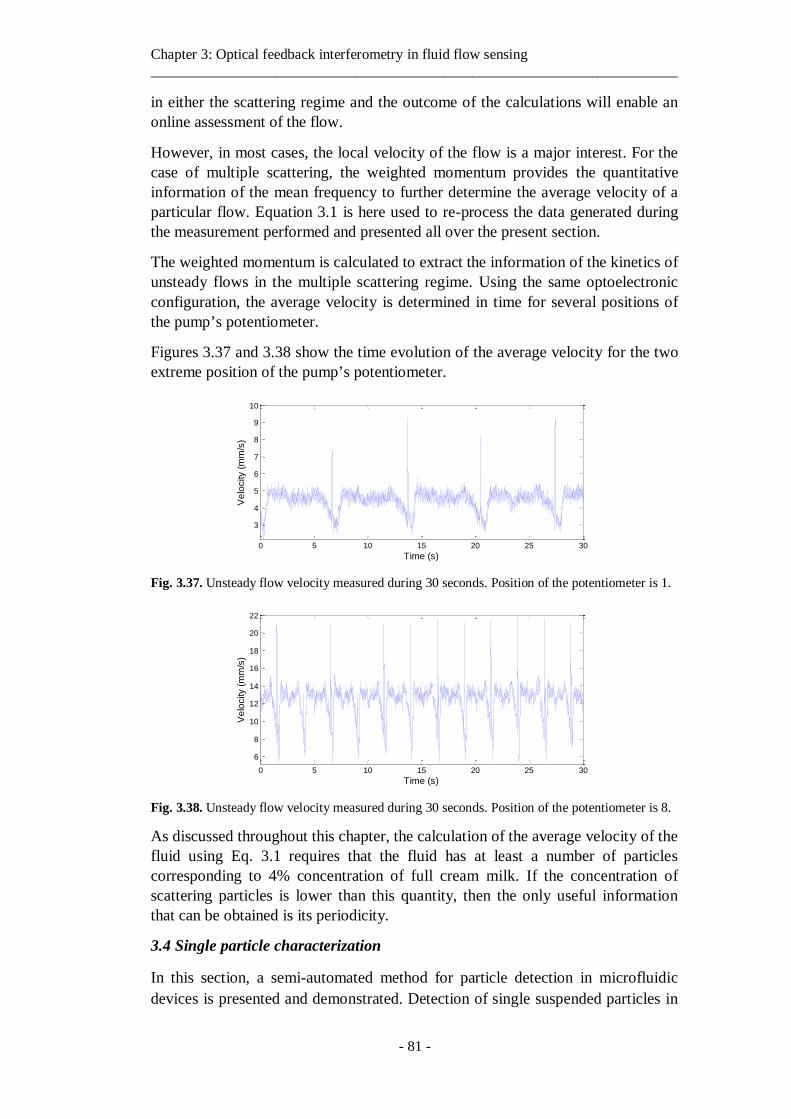
Chapter 3: Optical feedback interferometry in fluid flow sensing ________________________________________________________________________
- 81 -
in either the scattering regime and the outcome of the calculations will enable an
online assessment of the flow.
However, in most cases, the local velocity of the flow is a major interest. For the
case of multiple scattering, the weighted momentum provides the quantitative
information of the mean frequency to further determine the average velocity of a
particular flow. Equation 3.1 is here used to re-process the data generated during
the measurement performed and presented all over the present section.
The weighted momentum is calculated to extract the information of the kinetics of
unsteady flows in the multiple scattering regime. Using the same optoelectronic
configuration, the average velocity is determined in time for several positions of
the pump’s potentiometer.
Figures 3.37 and 3.38 show the time evolution of the average velocity for the two
extreme position of the pump’s potentiometer.
Fig. 3.37. Unsteady flow velocity measured during 30 seconds. Position of the potentiometer is 1.
Fig. 3.38. Unsteady flow velocity measured during 30 seconds. Position of the potentiometer is 8.
As discussed throughout this chapter, the calculation of the average velocity of the
fluid using Eq. 3.1 requires that the fluid has at least a number of particles
corresponding to 4% concentration of full cream milk. If the concentration of
scattering particles is lower than this quantity, then the only useful information
that can be obtained is its periodicity.
3.4 Single particle characterization
In this section, a semi-automated method for particle detection in microfluidic
devices is presented and demonstrated. Detection of single suspended particles in
0 5 10 15 20 25 30
3
4
5
6
7
8
9
10
Ve
locity (
mm
/s)
Time (s)
0 5 10 15 20 25 30
6
8
10
12
14
16
18
20
22
Ve
locity (
mm
/s)
Time (s)
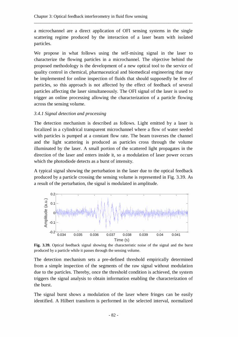
Chapter 3: Optical feedback interferometry in fluid flow sensing ________________________________________________________________________
- 82 -
a microchannel are a direct application of OFI sensing systems in the single
scattering regime produced by the interaction of a laser beam with isolated
particles.
We propose in what follows using the self-mixing signal in the laser to
characterize the flowing particles in a microchannel. The objective behind the
proposed methodology is the development of a new optical tool to the service of
quality control in chemical, pharmaceutical and biomedical engineering that may
be implemented for online inspection of fluids that should supposedly be free of
particles, so this approach is not affected by the effect of feedback of several
particles affecting the laser simultaneously. The OFI signal of the laser is used to
trigger an online processing allowing the characterization of a particle flowing
across the sensing volume.
3.4.1 Signal detection and processing
The detection mechanism is described as follows. Light emitted by a laser is
focalized in a cylindrical transparent microchannel where a flow of water seeded
with particles is pumped at a constant flow rate. The beam traverses the channel
and the light scattering is produced as particles cross through the volume
illuminated by the laser. A small portion of the scattered light propagates in the
direction of the laser and enters inside it, so a modulation of laser power occurs
which the photodiode detects as a burst of intensity.
A typical signal showing the perturbation in the laser due to the optical feedback
produced by a particle crossing the sensing volume is represented in Fig. 3.39. As
a result of the perturbation, the signal is modulated in amplitude.
Fig. 3.39. Optical feedback signal showing the characteristic noise of the signal and the burst
produced by a particle while it passes through the sensing volume.
The detection mechanism sets a pre-defined threshold empirically determined
from a simple inspection of the segments of the raw signal without modulation
due to the particles. Thereby, once the threshold condition is achieved, the system
triggers the signal analysis to obtain information enabling the characterization of
the burst.
The signal burst shows a modulation of the laser where fringes can be easily
identified. A Hilbert transform is performed in the selected interval, normalized
0.034 0.035 0.036 0.037 0.038 0.039 0.04 0.041-0.2
-0.1
0
0.1
0.2
Time (s)
Am
plit
ud
e (
a.u
.)
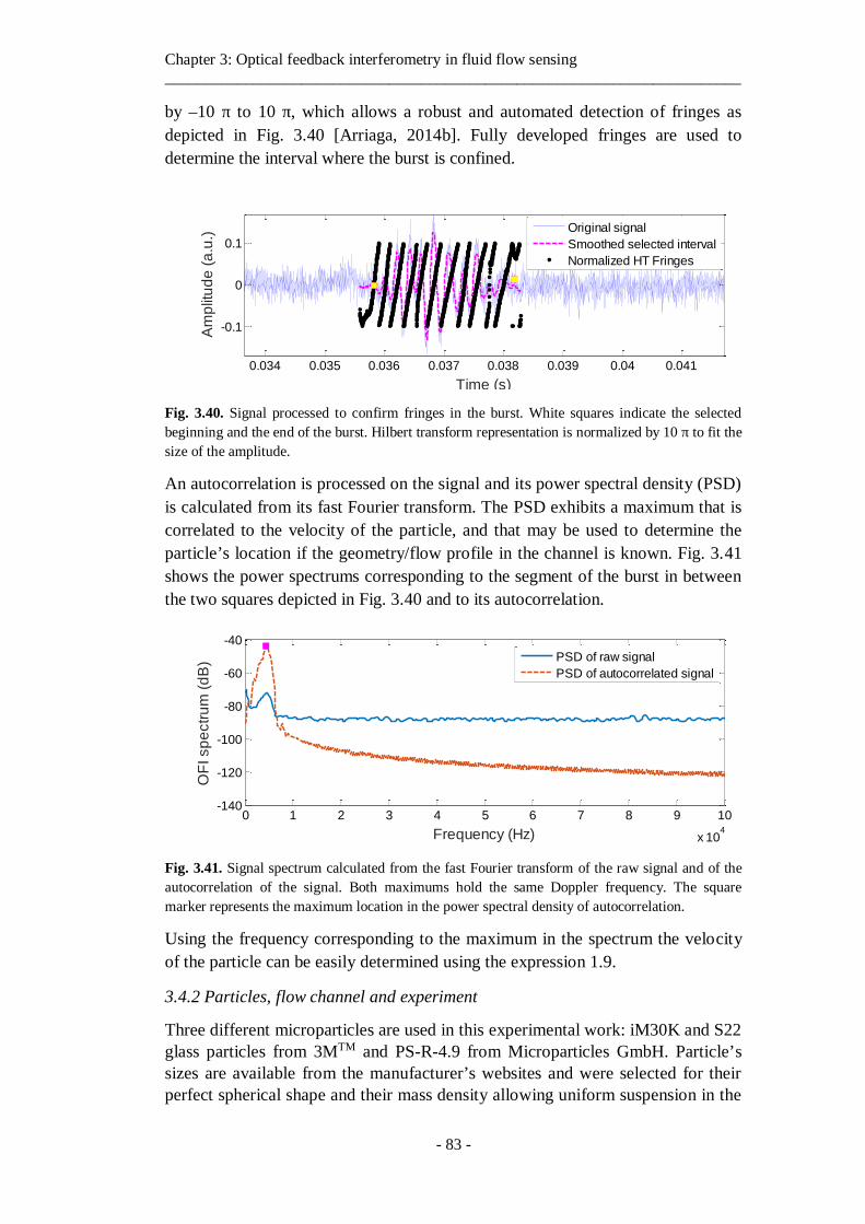
Chapter 3: Optical feedback interferometry in fluid flow sensing ________________________________________________________________________
- 83 -
by –10 π to 10 π, which allows a robust and automated detection of fringes as
depicted in Fig. 3.40 [Arriaga, 2014b]. Fully developed fringes are used to
determine the interval where the burst is confined.
Fig. 3.40. Signal processed to confirm fringes in the burst. White squares indicate the selected
beginning and the end of the burst. Hilbert transform representation is normalized by 10 π to fit the
size of the amplitude.
An autocorrelation is processed on the signal and its power spectral density (PSD)
is calculated from its fast Fourier transform. The PSD exhibits a maximum that is
correlated to the velocity of the particle, and that may be used to determine the
particle’s location if the geometry/flow profile in the channel is known. Fig. 3.41
shows the power spectrums corresponding to the segment of the burst in between
the two squares depicted in Fig. 3.40 and to its autocorrelation.
Fig. 3.41. Signal spectrum calculated from the fast Fourier transform of the raw signal and of the
autocorrelation of the signal. Both maximums hold the same Doppler frequency. The square
marker represents the maximum location in the power spectral density of autocorrelation.
Using the frequency corresponding to the maximum in the spectrum the velocity
of the particle can be easily determined using the expression 1.9.
3.4.2 Particles, flow channel and experiment
Three different microparticles are used in this experimental work: iM30K and S22
glass particles from 3MTM and PS-R-4.9 from Microparticles GmbH. Particle’s
sizes are available from the manufacturer’s websites and were selected for their
perfect spherical shape and their mass density allowing uniform suspension in the
0.034 0.035 0.036 0.037 0.038 0.039 0.04 0.041
-0.1
0
0.1
Time (s)
Am
plit
ud
e (
a.u
.)
Original signal
Smoothed selected interval
Normalized HT Fringes
0 1 2 3 4 5 6 7 8 9 10
x 104
-140
-120
-100
-80
-60
-40
Frequency (Hz)
OF
I sp
ectr
um
(d
B)
PSD of raw signal
PSD of autocorrelated signal
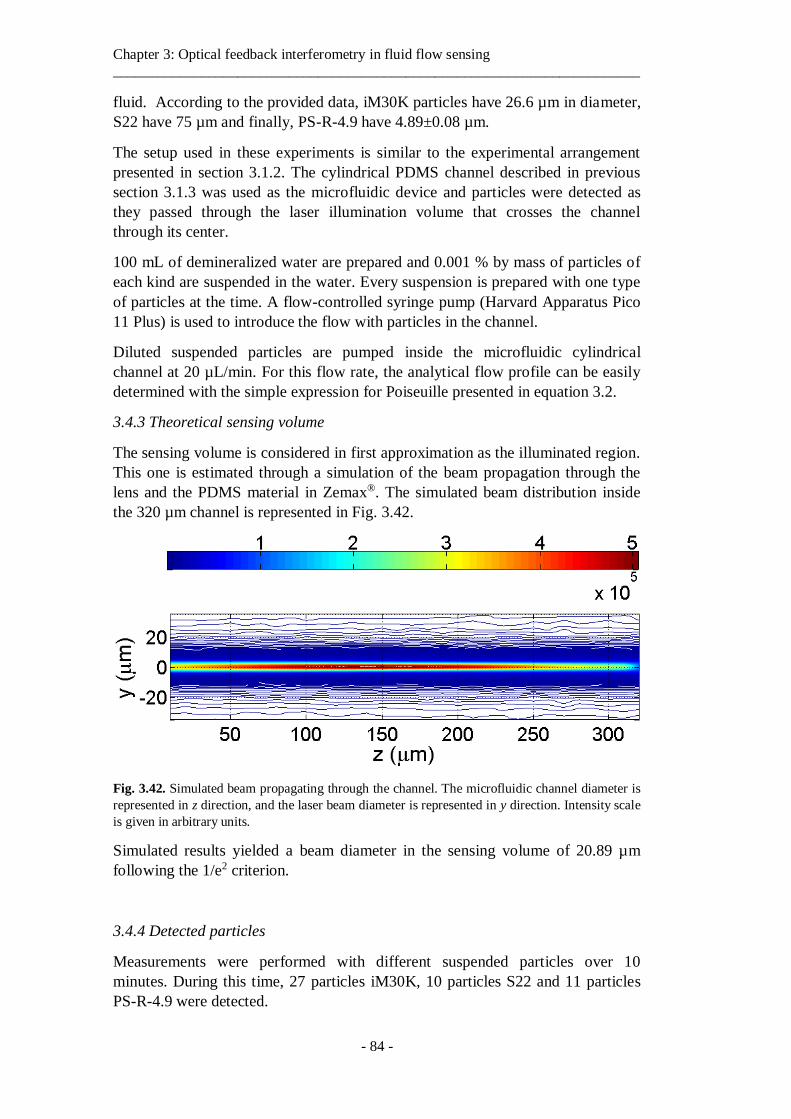
Chapter 3: Optical feedback interferometry in fluid flow sensing ________________________________________________________________________
- 84 -
fluid. According to the provided data, iM30K particles have 26.6 µm in diameter,
S22 have 75 µm and finally, PS-R-4.9 have 4.89±0.08 µm.
The setup used in these experiments is similar to the experimental arrangement
presented in section 3.1.2. The cylindrical PDMS channel described in previous
section 3.1.3 was used as the microfluidic device and particles were detected as
they passed through the laser illumination volume that crosses the channel
through its center.
100 mL of demineralized water are prepared and 0.001 % by mass of particles of
each kind are suspended in the water. Every suspension is prepared with one type
of particles at the time. A flow-controlled syringe pump (Harvard Apparatus Pico
11 Plus) is used to introduce the flow with particles in the channel.
Diluted suspended particles are pumped inside the microfluidic cylindrical
channel at 20 µL/min. For this flow rate, the analytical flow profile can be easily
determined with the simple expression for Poiseuille presented in equation 3.2.
3.4.3 Theoretical sensing volume
The sensing volume is considered in first approximation as the illuminated region.
This one is estimated through a simulation of the beam propagation through the
lens and the PDMS material in Zemax®. The simulated beam distribution inside
the 320 µm channel is represented in Fig. 3.42.
Fig. 3.42. Simulated beam propagating through the channel. The microfluidic channel diameter is
represented in z direction, and the laser beam diameter is represented in y direction. Intensity scale
is given in arbitrary units.
Simulated results yielded a beam diameter in the sensing volume of 20.89 µm
following the 1/e2 criterion.
3.4.4 Detected particles
Measurements were performed with different suspended particles over 10
minutes. During this time, 27 particles iM30K, 10 particles S22 and 11 particles
PS-R-4.9 were detected.
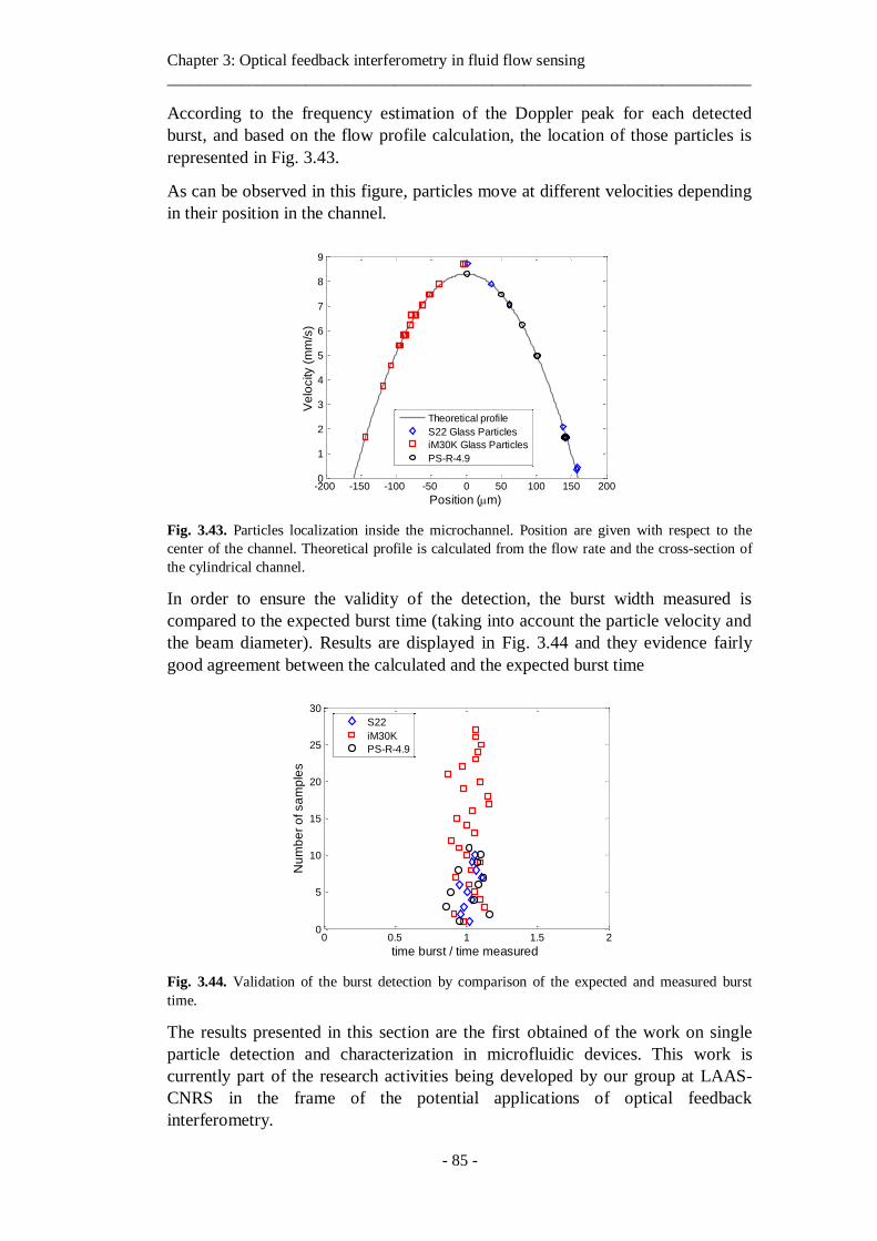
Chapter 3: Optical feedback interferometry in fluid flow sensing ________________________________________________________________________
- 85 -
According to the frequency estimation of the Doppler peak for each detected
burst, and based on the flow profile calculation, the location of those particles is
represented in Fig. 3.43.
As can be observed in this figure, particles move at different velocities depending
in their position in the channel.
Fig. 3.43. Particles localization inside the microchannel. Position are given with respect to the
center of the channel. Theoretical profile is calculated from the flow rate and the cross-section of
the cylindrical channel.
In order to ensure the validity of the detection, the burst width measured is
compared to the expected burst time (taking into account the particle velocity and
the beam diameter). Results are displayed in Fig. 3.44 and they evidence fairly
good agreement between the calculated and the expected burst time
Fig. 3.44. Validation of the burst detection by comparison of the expected and measured burst
time.
The results presented in this section are the first obtained of the work on single
particle detection and characterization in microfluidic devices. This work is
currently part of the research activities being developed by our group at LAAS-
CNRS in the frame of the potential applications of optical feedback
interferometry.
-200 -150 -100 -50 0 50 100 150 2000
1
2
3
4
5
6
7
8
9
Position (m)
Ve
locity (
mm
/s)
Theoretical profile
S22 Glass Particles
iM30K Glass Particles
PS-R-4.9
0 0.5 1 1.5 20
5
10
15
20
25
30
time burst / time measured
Nu
mb
er
of sa
mp
les
S22
iM30K
PS-R-4.9
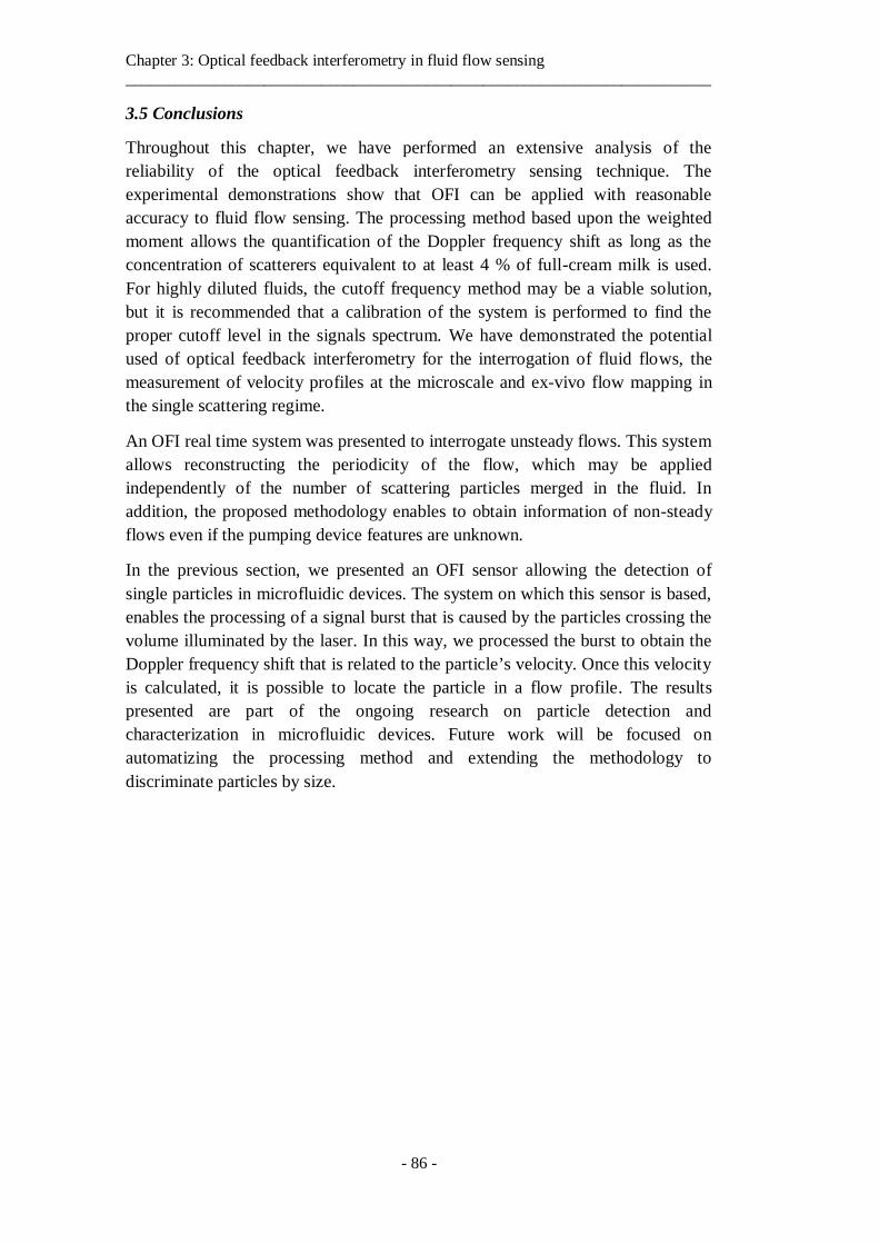
Chapter 3: Optical feedback interferometry in fluid flow sensing ________________________________________________________________________
- 86 -
3.5 Conclusions
Throughout this chapter, we have performed an extensive analysis of the
reliability of the optical feedback interferometry sensing technique. The
experimental demonstrations show that OFI can be applied with reasonable
accuracy to fluid flow sensing. The processing method based upon the weighted
moment allows the quantification of the Doppler frequency shift as long as the
concentration of scatterers equivalent to at least 4 % of full-cream milk is used.
For highly diluted fluids, the cutoff frequency method may be a viable solution,
but it is recommended that a calibration of the system is performed to find the
proper cutoff level in the signals spectrum. We have demonstrated the potential
used of optical feedback interferometry for the interrogation of fluid flows, the
measurement of velocity profiles at the microscale and ex-vivo flow mapping in
the single scattering regime.
An OFI real time system was presented to interrogate unsteady flows. This system
allows reconstructing the periodicity of the flow, which may be applied
independently of the number of scattering particles merged in the fluid. In
addition, the proposed methodology enables to obtain information of non-steady
flows even if the pumping device features are unknown.
In the previous section, we presented an OFI sensor allowing the detection of
single particles in microfluidic devices. The system on which this sensor is based,
enables the processing of a signal burst that is caused by the particles crossing the
volume illuminated by the laser. In this way, we processed the burst to obtain the
Doppler frequency shift that is related to the particle’s velocity. Once this velocity
is calculated, it is possible to locate the particle in a flow profile. The results
presented are part of the ongoing research on particle detection and
characterization in microfluidic devices. Future work will be focused on
automatizing the processing method and extending the methodology to
discriminate particles by size.
Chapter 4: Application of optical feedback interferometry to the analysis of multiphase
flows
- 87 -
Chapter 4
Application of optical feedback interferometry to the analysis of
multiphase flows
4.1 General context
Multiphase flows refer to flows carrying matter in different states. As per
definition, these flows are not restricted to a combination of substances
comprising different states of matter, so they are found in both gas-liquid
solutions and in liquid-liquid solutions [Brennen, 2005]. For the latter, it is
understood that the liquids hold different hydrodynamic properties.
Multiphase flows are present everywhere. The most obvious cases are seen every
day in clouds, snow and smoke, but also in food products of daily consumption
such as mayonnaise and salad dressing. Likewise, in water supply in domestic
services and in some type of drinking water, bubbly and sparkling flows are
notable. As early as 1950, it was found that adding up to 12 % of air into domestic
water would allow saving billions of liters of water a year, and would make the
water supply equally efficient, especially for cleaning purposes. Two-phase flows
intervene in multiple chemical and biochemical processes including mixing,
diffusion, cavitation and synthesis [Rudyak, 2014; Gordon, 2014; Rooze, 2012].
Still, multiphase flows are not limited to only two-phase flows. The oil extraction
Chapter 4: Application of optical feedback interferometry to the analysis of multiphase
flows
- 88 -
industry deals continuously with water, oil and gas in pipes transporting the
organic material [Taitel, 1995]. Three-phase flows have been subject of study
since many years, in both large scale and microscale engineering [Vinegar, 1987;
Oddie, 2003; Yue, 2014]. Also, solutions of detergent, soap and other foam-
forming substances are good examples of multiphase flows present in daily life.
Microfluidics continues to be an active area in research, covering a wide range of
applications in chemical, biological and medical engineering. The characterization
of fluid flows in microchannels has been particularly interesting for the scientific
community dedicated to microreactor technology. In this regard, the measurement
of physical parameters related to motion is still of great interest for the
interrogation of fluids at the micro-scale, with consequent impact on quality
control of industrial processes and on diagnostic purposes in biomedical field.
Additionally, microfluidics offers a complete platform to control and assess
chemical and biomedical processes that are too complex to be addressed at larger
scales. Typical microscale devices allow for flow assessment in laminar regime,
where experimentation and processes can be controlled. Moreover, interactions
between two laminar fluids at the microscale can be easily monitored and
interrogated. Just to mention a simple example, oil and water behave different in
large scale reservoir as compared to small pipes. These fluids are immiscible, and
normally at the macroscale oil floats in water due to its lower density. However,
when confined in a microchannel of a microfluidic chemical reactor, an oil-water
interface is created with such a surface tension that it remains vertical and fluids
develop parallel rather than stratified, where the gravity effect is not predominant.
So, using microfluidic chips to study immiscible fluids interactions is a suitable
tool for an easy inspection of motion related parameters in the hydrodynamics of
particular liquid-liquid interaction.
The configuration where two immiscible substances are flowing in the same
microchannel is subject of much current research [Raimondi, 2014]. In this
regard, the formation of droplets in microfluidic devices and the hydrodynamics
of slug flows have received extensive attention [Kashid, 2008]. In particular, the
scientific community devoted to microreactor engineering has projected great
efforts towards the study the dynamics of two phase liquid-liquid interactions. The
gold standard to characterize the interaction of two liquid flows at the microscale
is the analysis of flow patterns, but still there remains a large variety of liquid-
liquid interactions to be properly characterized [Foroughi, 2011].
To understand the liquid-liquid interactions (two-phase flow structure, mixing,
mass transfer, etc.), hydrodynamics parameters have to be determined. However,
measuring velocities in small dimension channels with acceptable accuracy is
challenging. Particle Image Velocimetry and Laser Doppler Velocimetry (LDV)
are currently used to measure velocity fields in large scale pipes [Kumara, 2010].
At present, the conventional technique to measure velocity fields at the microscale
Chapter 4: Application of optical feedback interferometry to the analysis of multiphase
flows
- 89 -
is the Micro Particle Image Velocimetry (μ-PIV). However, currently available μ-
PIV systems in their minimal configuration [Wereley, 2010] include a bulky high-
power pulsed Nd:YAG laser, a fast acquisition camera and a microscope system.
The tracers in the fluid have to be fluorescent particles. The optical arrangement
in μ-PIV requires that the vision field of the camera and the laser focus to be in
perfect correspondence and then implies a robust and precise alignment of all the
opto-mechanical assembly. Thus, μ-PIV are then heavy and expensive systems.
PIV requires the use of heavy equipment as a laser and a microscope that are
needed for flow quantification. In addition, is expensive and necessitates
advanced post-processing of images generated as flows are visualized. On the
other hand, LDV uses an interferometer with several optical components that
make its assembly unpractical for microchannel flow measurements. Imaging
systems are largely used in the study of multiphase flows. They allow tracking
and following the hydrodynamic system behavior under many possible
configurations. However, the assessment is usually subjective as a single-side
view of the channel is typically used. Imaging systems such as PIV and dual-slit
have been used as a powerful tool in assessing and quantifying flow behavior and
interactions. In a recent paper [Campagnolo, 2012], OFI technique was compared
to dual slit and both techniques successfully experimentally reproduced the flow
profile of a laminar flow in a rectangular microchannel. We will use the optical
visualization as a reference tool to confirm our experimental results obtained with
OFI in this chapter.
In previous chapters we have proven how Optical Feedback Interferometry (OFI)
can be used as a sensing method for velocity measurements. In addition, OFI
sensors for flows assessment were presented for those cases when the channel
contained only one fluid [Campagnolo, 2013a; Lim, 2010; Norgia, 2016].
However, OFI’s possible implementation in the analysis of multiphase flows is
still to be demonstrated. In this chapter we intend to fill the gap in the utilization if
OFI for the study of multiphase parallel liquid-liquid flows.
Pohar et al. [2012] demonstrated that when two parallel immiscible fluids interact
in a microchannel, they occupy a fraction of volume that depends directly on their
viscosity and the volume filled by every fluid is defined by the interface between
the flows. In the case of parallel oil-water flows, each phase develops its own
velocity profile and the interface can be displaced by changing the flow rate at the
inlets. The demonstration of the effect of viscosity on the hydrodynamics of
parallel flows relies on a visualization of the transparent channel, thus the
information provided by images is sufficient to determine the volume occupied by
each fluid in the channel.
As a first approach, we drove our attention towards velocity measurements of oil-
water parallel flows in a Y-shaped microreactor and tested the OFI sensing
technique as a tool to characterize two-phase parallel flows and to estimate the
Chapter 4: Application of optical feedback interferometry to the analysis of multiphase
flows
- 90 -
location of the interface separating immiscible fluids in a microchannel. Parallel
flows are the simplest case of liquid-liquid immiscible interactions. In this
chapter, we will demonstrate the potential of OFI in the analysis of oil-water
flows departing from a characterization of motion-related parameters allowing
velocity profiles measurements. Since velocity is related to flow distribution, it
can be used as a parameter to estimate and localize the interface of oil-water
immiscible flows in a microchannel. We present experimental results of velocity
profile measurements and explore the impact of changes in the water flow rate.
Indeed the latter provides valuable quantitative information on the spatial
repartition of the fluids. In addition, we use the OFI sensing scheme to interrogate
the flow profiles while maintaining constant the ratio of flow rates imposed at the
inlets. Under such conditions, the interface position is expected to remain
unchanged.
Experimentally obtained velocity profiles can be fitted to a theoretical
approximation considering oil and water as viscous fluids. In this approximation,
the interaction of both immiscible fluids is characterized by the influence of a
pressure gradient and viscosity in the kinetics of each parallel flow. As a
consequence, a theoretical model that considers oil and water as viscous fluids is
proposed to describe the the possible influence of one phase on the other. It is
based on the Couette flows approximation and is compared to the experimental
results.
4.2 Theoretical model of parallel liquid-liquid flows
As mentioned in the previous section of this chapter, the hydrodynamics of two
immiscible fluids in a microchannel can be described by modeling the possible
influence of one fluid on the other. As both fluids move under a pressure gradient,
the kinetics is influenced by the pressure drop imposed by the pumps at the inlets.
In such a case, fluids occupy a portion of volume in the channel that is highly
dependent on the intrinsic properties of the fluids, particularly their viscosity.
In an attempt to address the influence of one liquid on the other and the role of the
interface separating them, we first present a basic theory on the type of flows
considered in the theoretical approach presented in this section. Thereby, we
introduce the concept of Couette flows and its suitability to describe the oil-water
system hydrodynamics.
Couette flows are considered as confined fluids into two parallel plates subject to
the relative movement of one of the plates respect to the other. In such a case, the
velocity of the flow in one of its spatial boundaries is different from zero. Figure
4.1 present a schematic representation of the situation that will help understand
the general concept. If a fluid at rest is pushed by the action of one of the wall that
confined it, then a dragging effect will affect the velocity distribution of the flow
with a maximum velocity in the moving plate.
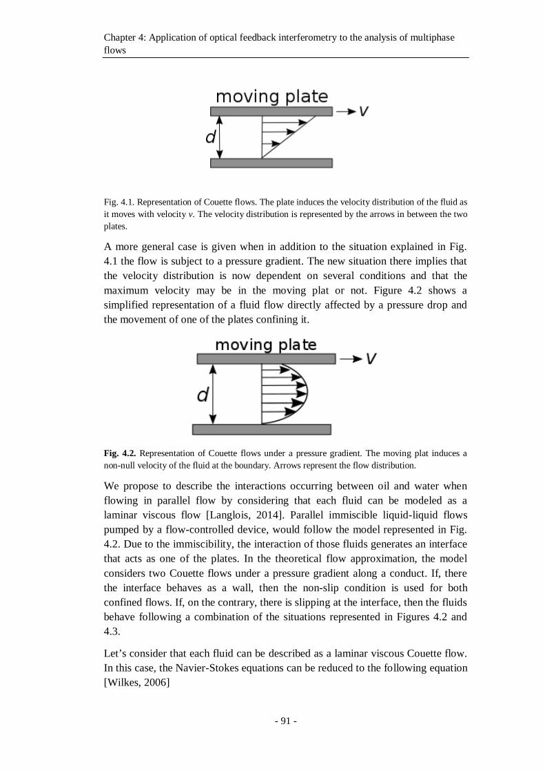
Chapter 4: Application of optical feedback interferometry to the analysis of multiphase
flows
- 91 -
Fig. 4.1. Representation of Couette flows. The plate induces the velocity distribution of the fluid as
it moves with velocity v. The velocity distribution is represented by the arrows in between the two
plates.
A more general case is given when in addition to the situation explained in Fig.
4.1 the flow is subject to a pressure gradient. The new situation there implies that
the velocity distribution is now dependent on several conditions and that the
maximum velocity may be in the moving plat or not. Figure 4.2 shows a
simplified representation of a fluid flow directly affected by a pressure drop and
the movement of one of the plates confining it.
Fig. 4.2. Representation of Couette flows under a pressure gradient. The moving plat induces a
non-null velocity of the fluid at the boundary. Arrows represent the flow distribution.
We propose to describe the interactions occurring between oil and water when
flowing in parallel flow by considering that each fluid can be modeled as a
laminar viscous flow [Langlois, 2014]. Parallel immiscible liquid-liquid flows
pumped by a flow-controlled device, would follow the model represented in Fig.
4.2. Due to the immiscibility, the interaction of those fluids generates an interface
that acts as one of the plates. In the theoretical flow approximation, the model
considers two Couette flows under a pressure gradient along a conduct. If, there
the interface behaves as a wall, then the non-slip condition is used for both
confined flows. If, on the contrary, there is slipping at the interface, then the fluids
behave following a combination of the situations represented in Figures 4.2 and
4.3.
Let’s consider that each fluid can be described as a laminar viscous Couette flow.
In this case, the Navier-Stokes equations can be reduced to the following equation
[Wilkes, 2006]
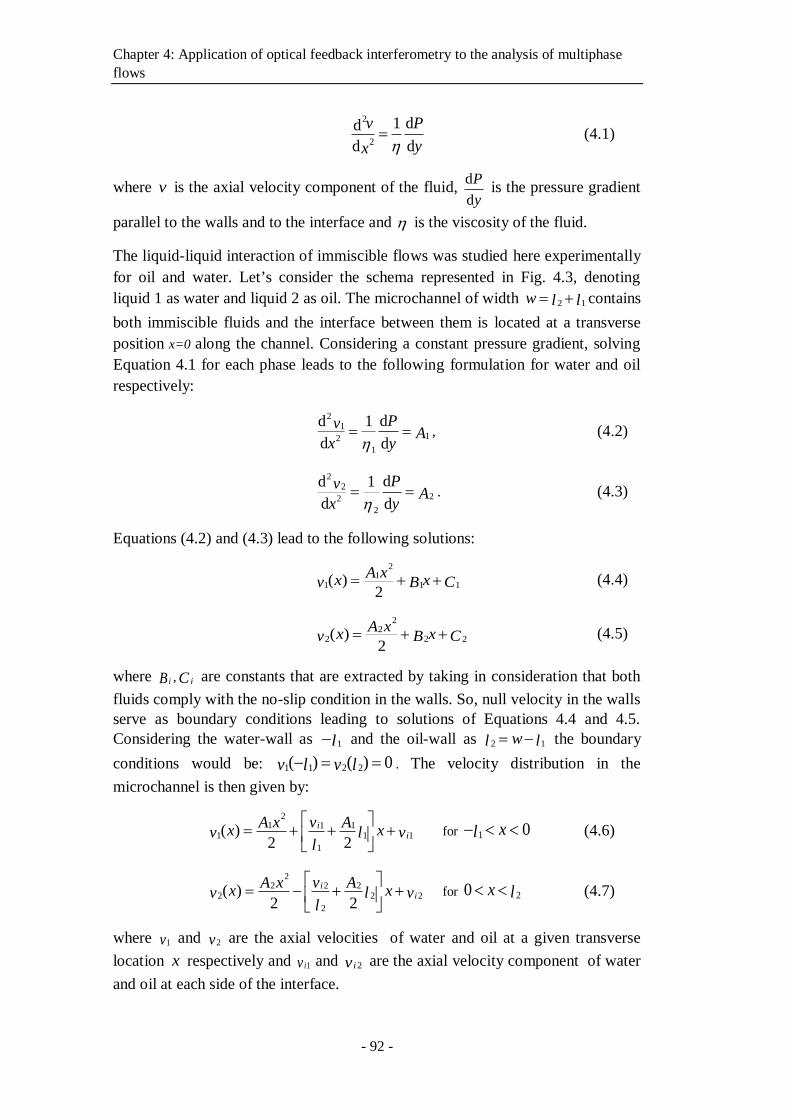
Chapter 4: Application of optical feedback interferometry to the analysis of multiphase
flows
- 92 -
2
2
1 dd
d d
v P
yx (4.1)
where v is the axial velocity component of the fluid, d
d
P
y is the pressure gradient
parallel to the walls and to the interface and is the viscosity of the fluid.
The liquid-liquid interaction of immiscible flows was studied here experimentally
for oil and water. Let’s consider the schema represented in Fig. 4.3, denoting
liquid 1 as water and liquid 2 as oil. The microchannel of width 2 1w l l contains
both immiscible fluids and the interface between them is located at a transverse
position x=0 along the channel. Considering a constant pressure gradient, solving
Equation 4.1 for each phase leads to the following formulation for water and oil
respectively:
21
12
1
dd 1
d d
PvA
x y , (4.2)
22
22
2
dd 1
d d
PvA
x y . (4.3)
Equations (4.2) and (4.3) lead to the following solutions:
21
11 1( )2
xAx xv CB (4.4)
22
22 2( )2
xAx xv CB (4.5)
where iB , iC are constants that are extracted by taking in consideration that both
fluids comply with the no-slip condition in the walls. So, null velocity in the walls
serve as boundary conditions leading to solutions of Equations 4.4 and 4.5.
Considering the water-wall as 1l and the oil-wall as 2 1wl l the boundary
conditions would be: 1 1 2 2( ) ( ) 0v l v l . The velocity distribution in the
microchannel is then given by:
21 11
1 1 1
1
( )2 2
ii
x vA Ax xv l v
l
for 1 0xl (4.6)
22 22
2 2 2
2
( )2 2
ii
x vA Ax xv l v
l
for 20 x l (4.7)
where 1v and 2v are the axial velocities of water and oil at a given transverse
location x respectively and 1iv and 2iv are the axial velocity component of water
and oil at each side of the interface.
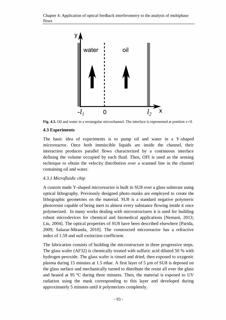
Chapter 4: Application of optical feedback interferometry to the analysis of multiphase
flows
- 93 -
Fig. 4.3. Oil and water in a rectangular microchannel. The interface is represented at position x=0.
4.3 Experiments
The basic idea of experiments is to pump oil and water in a Y-shaped
microreactor. Once both immiscible liquids are inside the channel, their
interaction produces parallel flows characterized by a continuous interface
defining the volume occupied by each fluid. Then, OFI is used as the sensing
technique to obtain the velocity distribution over a scanned line in the channel
containing oil and water.
4.3.1 Microfluidic chip
A custom made Y-shaped microreactor is built in SU8 over a glass substrate using
optical lithography. Previously designed photo-masks are employed to create the
lithographic geometries on the material. SU8 is a standard negative polymeric
photoresist capable of being inert to almost every substance flowing inside it once
polymerized. In many works dealing with microstructures it is used for building
robust microdevices for chemical and biomedical applications [Nemani, 2013;
Liu, 2004]. The optical properties of SU8 have been described elsewhere [Parida,
2009; Salazar-Miranda, 2010]. The constructed microreactor has a refractive
index of 1.59 and null extinction coefficient.
The fabrication consists of building the microstructure in three progressive steps.
The glass wafer (AF32) is chemically treated with sulfuric acid diluted 50 % with
hydrogen peroxide. The glass wafer is rinsed and dried, then exposed to oxygenic
plasma during 15 minutes at 1.5 mbar. A first layer of 5 μm of SU8 is deposed on
the glass surface and mechanically turned to distribute the resist all over the glass
and heated at 95 ºC during three minutes. Then, the material is exposed to UV
radiation using the mask corresponding to this layer and developed during
approximately 5 minutes until it polymerizes completely.
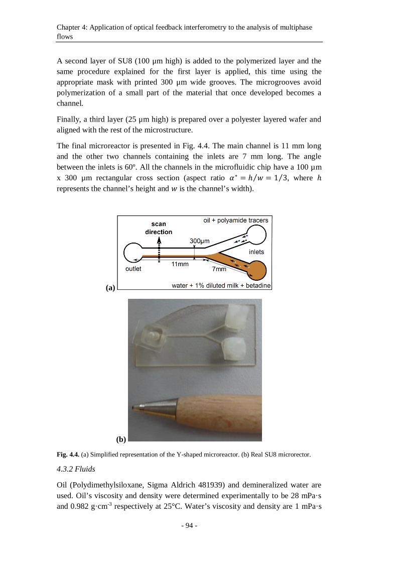
Chapter 4: Application of optical feedback interferometry to the analysis of multiphase
flows
- 94 -
A second layer of SU8 (100 μm high) is added to the polymerized layer and the
same procedure explained for the first layer is applied, this time using the
appropriate mask with printed 300 μm wide grooves. The microgrooves avoid
polymerization of a small part of the material that once developed becomes a
channel.
Finally, a third layer (25 μm high) is prepared over a polyester layered wafer and
aligned with the rest of the microstructure.
The final microreactor is presented in Fig. 4.4. The main channel is 11 mm long
and the other two channels containing the inlets are 7 mm long. The angle
between the inlets is 60º. All the channels in the microfluidic chip have a 100 µm
x 300 µm rectangular cross section (aspect ratio 𝛼∗ = ℎ 𝑤⁄ = 1 3⁄ , where ℎ
represents the channel’s height and 𝑤 is the channel’s width).
(a)
(b)
Fig. 4.4. (a) Simplified representation of the Y-shaped microreactor. (b) Real SU8 microrector.
4.3.2 Fluids
Oil (Polydimethylsiloxane, Sigma Aldrich 481939) and demineralized water are
used. Oil’s viscosity and density were determined experimentally to be 28 mPa·s
and 0.982 g·cm-3 respectively at 25°C. Water’s viscosity and density are 1 mPa·s
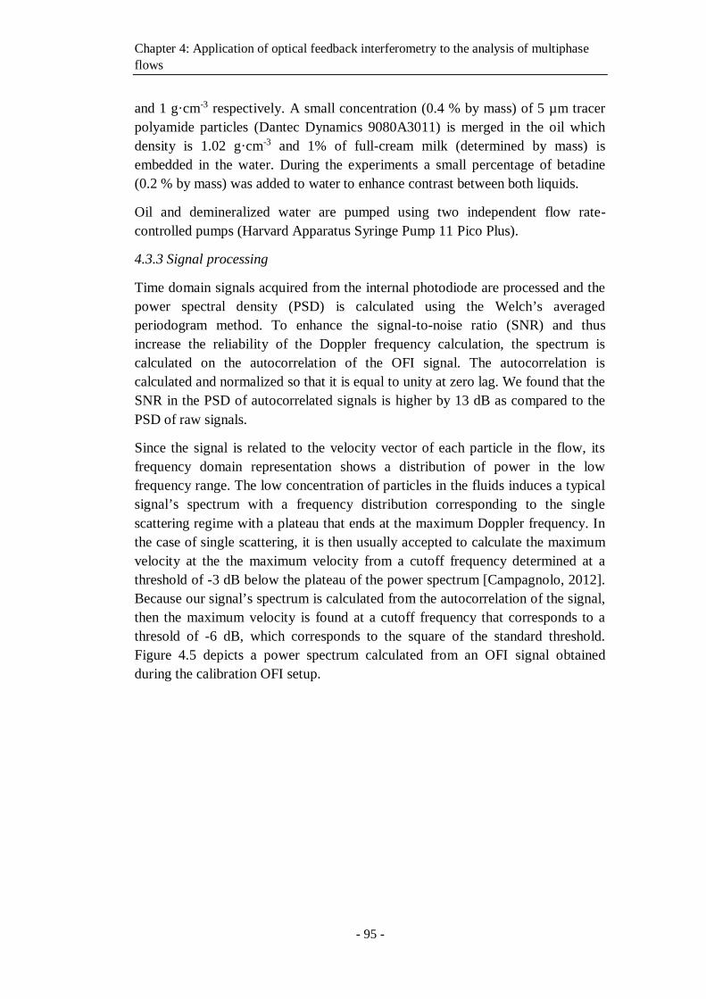
Chapter 4: Application of optical feedback interferometry to the analysis of multiphase
flows
- 95 -
and 1 g·cm-3 respectively. A small concentration (0.4 % by mass) of 5 µm tracer
polyamide particles (Dantec Dynamics 9080A3011) is merged in the oil which
density is 1.02 g·cm-3 and 1% of full-cream milk (determined by mass) is
embedded in the water. During the experiments a small percentage of betadine
(0.2 % by mass) was added to water to enhance contrast between both liquids.
Oil and demineralized water are pumped using two independent flow rate-
controlled pumps (Harvard Apparatus Syringe Pump 11 Pico Plus).
4.3.3 Signal processing
Time domain signals acquired from the internal photodiode are processed and the
power spectral density (PSD) is calculated using the Welch’s averaged
periodogram method. To enhance the signal-to-noise ratio (SNR) and thus
increase the reliability of the Doppler frequency calculation, the spectrum is
calculated on the autocorrelation of the OFI signal. The autocorrelation is
calculated and normalized so that it is equal to unity at zero lag. We found that the
SNR in the PSD of autocorrelated signals is higher by 13 dB as compared to the
PSD of raw signals.
Since the signal is related to the velocity vector of each particle in the flow, its
frequency domain representation shows a distribution of power in the low
frequency range. The low concentration of particles in the fluids induces a typical
signal’s spectrum with a frequency distribution corresponding to the single
scattering regime with a plateau that ends at the maximum Doppler frequency. In
the case of single scattering, it is then usually accepted to calculate the maximum
velocity at the the maximum velocity from a cutoff frequency determined at a
threshold of -3 dB below the plateau of the power spectrum [Campagnolo, 2012].
Because our signal’s spectrum is calculated from the autocorrelation of the signal,
then the maximum velocity is found at a cutoff frequency that corresponds to a
thresold of -6 dB, which corresponds to the square of the standard threshold.
Figure 4.5 depicts a power spectrum calculated from an OFI signal obtained
during the calibration OFI setup.
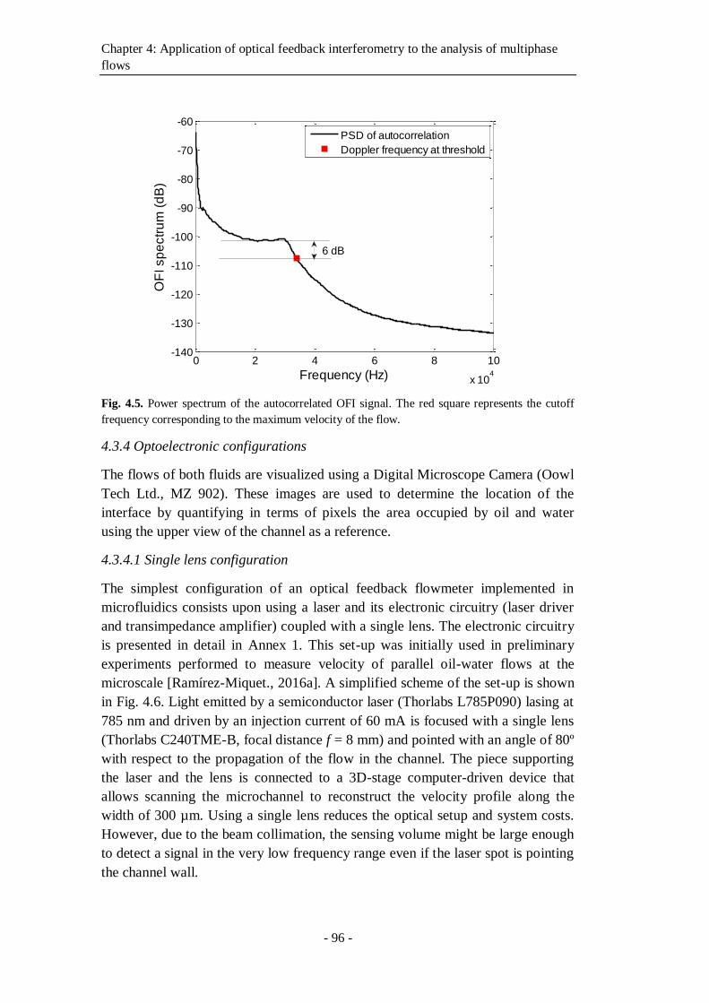
Chapter 4: Application of optical feedback interferometry to the analysis of multiphase
flows
- 96 -
Fig. 4.5. Power spectrum of the autocorrelated OFI signal. The red square represents the cutoff
frequency corresponding to the maximum velocity of the flow.
4.3.4 Optoelectronic configurations
The flows of both fluids are visualized using a Digital Microscope Camera (Oowl
Tech Ltd., MZ 902). These images are used to determine the location of the
interface by quantifying in terms of pixels the area occupied by oil and water
using the upper view of the channel as a reference.
4.3.4.1 Single lens configuration
The simplest configuration of an optical feedback flowmeter implemented in
microfluidics consists upon using a laser and its electronic circuitry (laser driver
and transimpedance amplifier) coupled with a single lens. The electronic circuitry
is presented in detail in Annex 1. This set-up was initially used in preliminary
experiments performed to measure velocity of parallel oil-water flows at the
microscale [Ramírez-Miquet., 2016a]. A simplified scheme of the set-up is shown
in Fig. 4.6. Light emitted by a semiconductor laser (Thorlabs L785P090) lasing at
785 nm and driven by an injection current of 60 mA is focused with a single lens
(Thorlabs C240TME-B, focal distance f = 8 mm) and pointed with an angle of 80º
with respect to the propagation of the flow in the channel. The piece supporting
the laser and the lens is connected to a 3D-stage computer-driven device that
allows scanning the microchannel to reconstruct the velocity profile along the
width of 300 µm. Using a single lens reduces the optical setup and system costs.
However, due to the beam collimation, the sensing volume might be large enough
to detect a signal in the very low frequency range even if the laser spot is pointing
the channel wall.
0 2 4 6 8 10
x 104
-140
-130
-120
-110
-100
-90
-80
-70
-60
Frequency (Hz)
OF
I sp
ectr
um
(d
B)
PSD of autocorrelation
Doppler frequency at threshold
6 dB
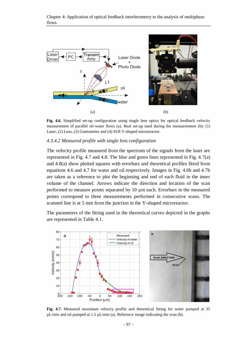
Chapter 4: Application of optical feedback interferometry to the analysis of multiphase
flows
- 97 -
(a) (b)
Fig. 4.6. Simplified set-up configuration using single lens optics for optical feedback velocity
measurement of parallel oil-water flows (a). Real set-up used during the measurements (b): (1)
Laser, (2) Lens, (3) Goniometer and (4) SU8 Y-shaped microreactor.
4.3.4.2 Measured profile with single lens configuration
The velocity profile measured from the spectrum of the signals from the laser are
represented in Fig. 4.7 and 4.8. The blue and green lines represented in Fig. 4.7(a)
and 4.8(a) show plotted squares with errorbars and theoretical profiles fitted from
equations 4.6 and 4.7 for water and oil respectively. Images in Fig. 4.6b and 4.7b
are taken as a reference to plot the beginning and end of each fluid in the inner
volume of the channel. Arrows indicate the direction and location of the scan
performed to measure points separated by 10 µm each. Errorbars in the measured
points correspond to three measurements performed in consecutive scans. The
scanned line is at 5 mm from the junction in the Y-shaped microreactor.
The parameters of the fitting used in the theoretical curves depicted in the graphs
are represented in Table 4.1.
Fig. 4.7. Measured maximum velocity profile and theoretical fitting for water pumped at 35
µL/min and oil pumped at 1.5 µL/min (a). Reference image indicating the scan (b).
-200 -150 -100 -50 0 50 100 150 2000
10
20
30
40
50
60
70
80
Position (m)
Ve
locity (
mm
/s)
Measured
Velocity of water
Velocity of oil
a
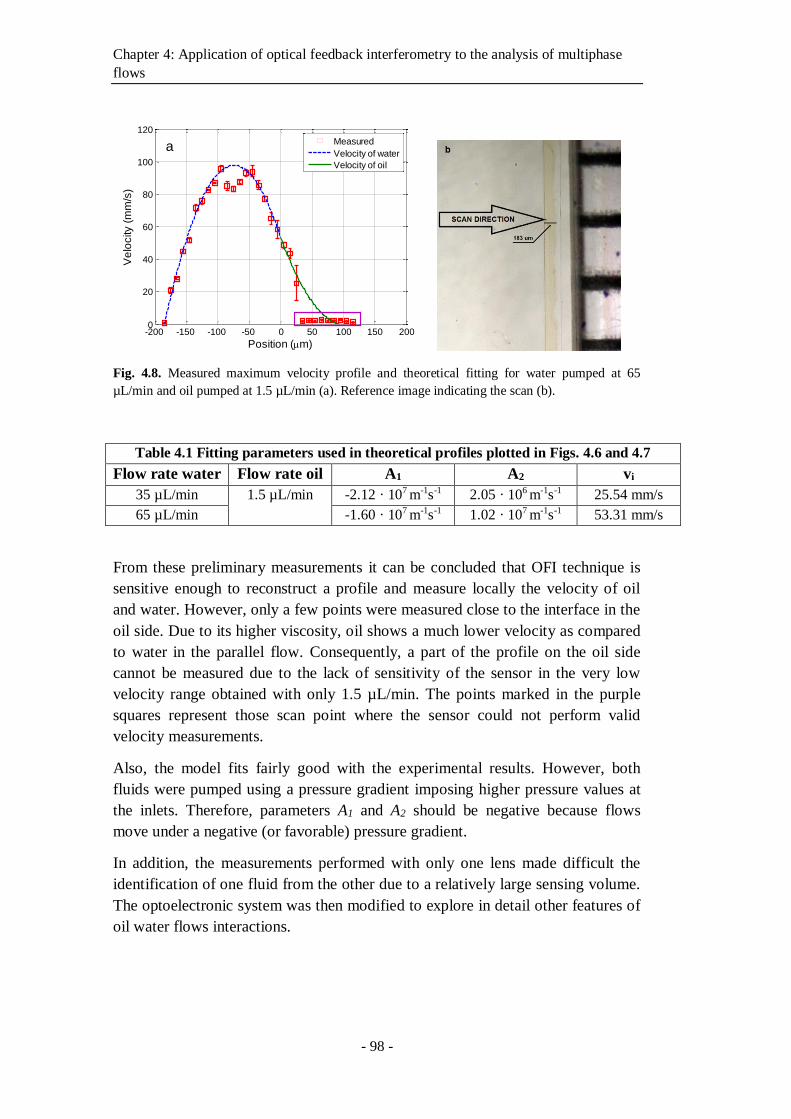
Chapter 4: Application of optical feedback interferometry to the analysis of multiphase
flows
- 98 -
Fig. 4.8. Measured maximum velocity profile and theoretical fitting for water pumped at 65
µL/min and oil pumped at 1.5 µL/min (a). Reference image indicating the scan (b).
From these preliminary measurements it can be concluded that OFI technique is
sensitive enough to reconstruct a profile and measure locally the velocity of oil
and water. However, only a few points were measured close to the interface in the
oil side. Due to its higher viscosity, oil shows a much lower velocity as compared
to water in the parallel flow. Consequently, a part of the profile on the oil side
cannot be measured due to the lack of sensitivity of the sensor in the very low
velocity range obtained with only 1.5 µL/min. The points marked in the purple
squares represent those scan point where the sensor could not perform valid
velocity measurements.
Also, the model fits fairly good with the experimental results. However, both
fluids were pumped using a pressure gradient imposing higher pressure values at
the inlets. Therefore, parameters A1 and A2 should be negative because flows
move under a negative (or favorable) pressure gradient.
In addition, the measurements performed with only one lens made difficult the
identification of one fluid from the other due to a relatively large sensing volume.
The optoelectronic system was then modified to explore in detail other features of
oil water flows interactions.
-200 -150 -100 -50 0 50 100 150 2000
20
40
60
80
100
120
Position (m)
Ve
locity (
mm
/s)
Measured
Velocity of water
Velocity of oil
a
Table 4.1 Fitting parameters used in theoretical profiles plotted in Figs. 4.6 and 4.7
Flow rate water Flow rate oil A1 A2 vi
35 µL/min 1.5 µL/min -2.12 · 107 m-1s-1 2.05 · 106 m-1s-1 25.54 mm/s
65 µL/min -1.60 · 107 m-1s-1 1.02 · 107 m-1s-1 53.31 mm/s
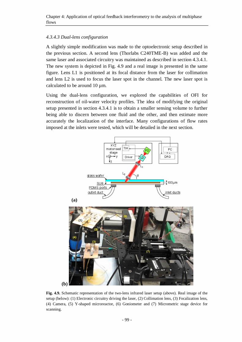
Chapter 4: Application of optical feedback interferometry to the analysis of multiphase
flows
- 99 -
4.3.4.3 Dual-lens configuration
A slightly simple modification was made to the optoelectronic setup described in
the previous section. A second lens (Thorlabs C240TME-B) was added and the
same laser and associated circuitry was maintained as described in section 4.3.4.1.
The new system is depicted in Fig. 4.9 and a real image is presented in the same
figure. Lens L1 is positioned at its focal distance from the laser for collimation
and lens L2 is used to focus the laser spot in the channel. The new laser spot is
calculated to be around 10 µm.
Using the dual-lens configuration, we explored the capabilities of OFI for
reconstruction of oil-water velocity profiles. The idea of modifying the original
setup presented in section 4.3.4.1 is to obtain a smaller sensing volume to further
being able to discern between one fluid and the other, and then estimate more
accurately the localization of the interface. Many configurations of flow rates
imposed at the inlets were tested, which will be detailed in the next section.
(a)
(b)
Fig. 4.9. Schematic representation of the two-lens infrared laser setup (above). Real image of the
setup (below): (1) Electronic circuitry driving the laser, (2) Collimation lens, (3) Focalization lens,
(4) Camera, (5) Y-shaped microreactor, (6) Goniometer and (7) Micrometric stage device for
scanning.
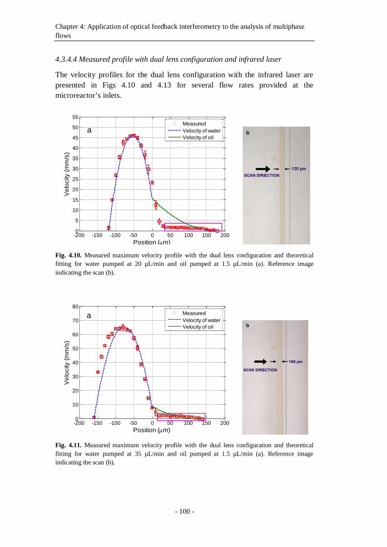
Chapter 4: Application of optical feedback interferometry to the analysis of multiphase
flows
- 100 -
4.3.4.4 Measured profile with dual lens configuration and infrared laser
The velocity profiles for the dual lens configuration with the infrared laser are
presented in Figs 4.10 and 4.13 for several flow rates provided at the
microreactor’s inlets.
Fig. 4.10. Measured maximum velocity profile with the dual lens configuration and theoretical
fitting for water pumped at 20 µL/min and oil pumped at 1.5 µL/min (a). Reference image
indicating the scan (b).
Fig. 4.11. Measured maximum velocity profile with the dual lens configuration and theoretical
fitting for water pumped at 35 µL/min and oil pumped at 1.5 µL/min (a). Reference image
indicating the scan (b).
-200 -150 -100 -50 0 50 100 150 2000
5
10
15
20
25
30
35
40
45
50
55
Position (m)
Ve
locity (
mm
/s)
Measured
Velocity of water
Velocity of oil
a
-200 -150 -100 -50 0 50 100 150 2000
10
20
30
40
50
60
70
80
Position (m)
Ve
locity (
mm
/s)
Measured
Velocity of water
Velocity of oil
a
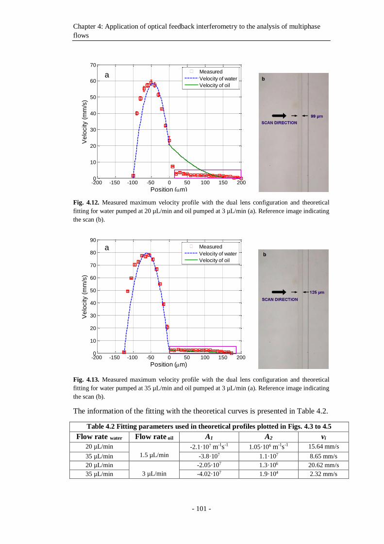
Chapter 4: Application of optical feedback interferometry to the analysis of multiphase
flows
- 101 -
Fig. 4.12. Measured maximum velocity profile with the dual lens configuration and theoretical
fitting for water pumped at 20 µL/min and oil pumped at 3 µL/min (a). Reference image indicating
the scan (b).
Fig. 4.13. Measured maximum velocity profile with the dual lens configuration and theoretical
fitting for water pumped at 35 µL/min and oil pumped at 3 µL/min (a). Reference image indicating
the scan (b).
The information of the fitting with the theoretical curves is presented in Table 4.2.
Table 4.2 Fitting parameters used in theoretical profiles plotted in Figs. 4.3 to 4.5
Flow rate water Flow rate oil A1 A2 vi
20 µL/min
1.5 µL/min
-2.1·107 m-1s-1 1.05·106 m-1s-1 15.64 mm/s
35 µL/min -3.8·107 1.1·107 8.65 mm/s
20 µL/min
3 µL/min
-2.05·107 1.3·106 20.62 mm/s
35 µL/min -4.02·107 1.9·104 2.32 mm/s
-200 -150 -100 -50 0 50 100 150 2000
10
20
30
40
50
60
70
Position (m)
Ve
locity (
mm
/s)
Measured
Velocity of water
Velocity of oil
a
-200 -150 -100 -50 0 50 100 150 2000
10
20
30
40
50
60
70
80
90
Position (m)
Ve
locity (
mm
/s)
Measured
Velocity of water
Velocity of oil
a
Chapter 4: Application of optical feedback interferometry to the analysis of multiphase
flows
- 102 -
All profiles represented in all tested configurations show that OFI can be used
with success in profiling water flow, but still the sensor lacks enough sensitivity to
perform valid velocity measurements in the oil. Nevertheless, the two-lens
configuration evidences more precisely the possible location of the interface.
From this set of measurements can be concluded that the laser wavelength is
probably too long to detect slow velocities as those corresponding to oil. The
maximum flow rate used (3 µL/min) is too slow to generate a detectable signal
with the infrared laser. In all figures, those points inside the purple rectangle could
not be properly measured and velocities values are inaccurate. This situation
imposes a redesign of the OFI sensor to make a new configuration capable of
detecting useful signals all over the scanned line that may fit a theoretical profile
for oil with negative pressure gradient contained in parameter A2. Also, it will be
important to have accurate measurements to have a better understanding of the
velocities at each side of the interface. This will allows us to understand how the
velocity profiles are developed and how their interaction may affect the behavior
of both fluids.
4.3.4.5 Measured profile with dual-lens configuration and blue-violet laser
In previous sections we have shown how an OFI flowmeter based upon an
infrared laser can perform accurate measurements of water flowing at several tens
of uL/min in a chemical microreactor. However, in the study of oil-water flows in
the same small channel, no valid velocity measurements could be done to fully
reconstruct the profile of both parallel fluids.
The real experimental set-up is shown in Figure 4.14 and the simplified
representation of the setup is consistent with the diagram shown in Fig. 4.6. It
consists of a blue-violet laser diode (Panasonic DL-5146-101S) with a short
wavelength λ=405 nm. Kliese [2010] demonstrated that OFI flow sensors
incorporating lasers with shorter wavelength are capable to measure very slow
velocities, out of the range that an infrared laser would detect. The OFI sensor is
coupled to two lenses (Thorlabs C240TM-A). Lens L1 is used for collimation
while the lens L2 is dedicated to the focalization at the microchannel’s center in
depth. The laser spot size obtained with this configuration has been calculated
with a ray tracing software, and is expected to be around 9 µm in diameter
according to the 1/e2 criterion. The electronic circuitry relative to this laser is
presented in Annex 2.
At first, in order to vary the position of the interface between both fluids, the flow
rate of water (Qwater) varies from 20 µL/min to 65 µL/min in steps of 15 µL/min
while the flow rate of oil (Qoil) was fixed at 3 µL/min.
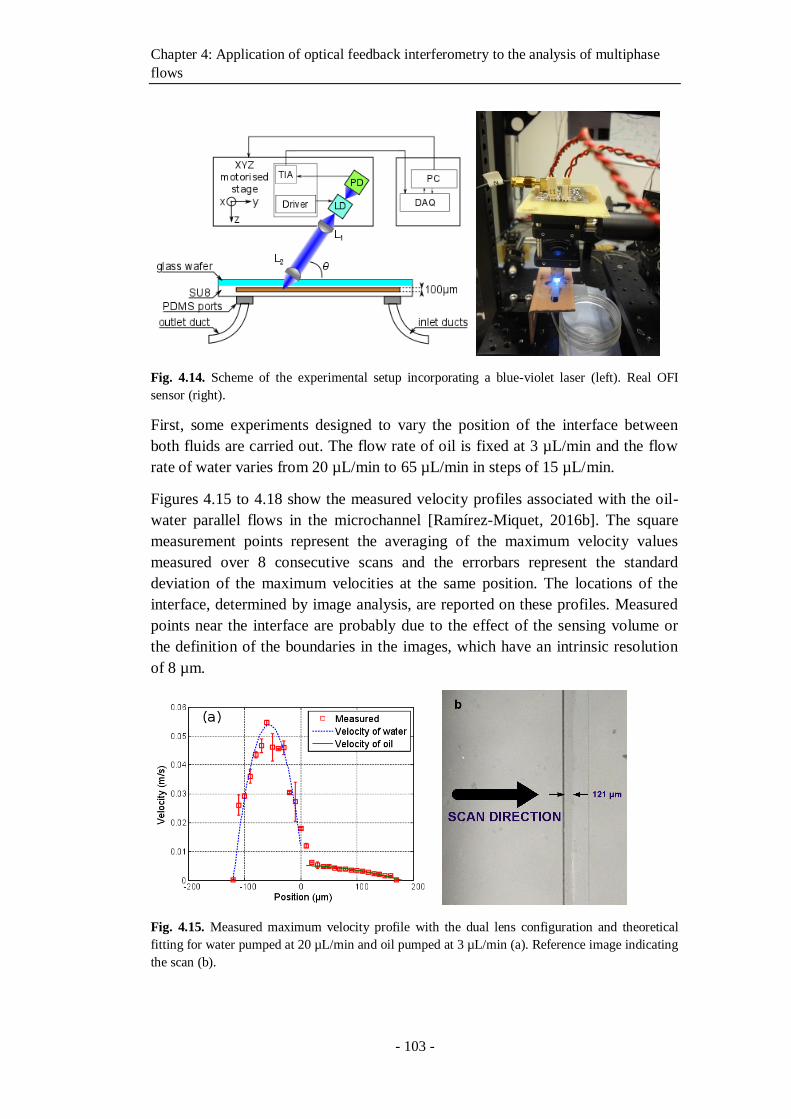
Chapter 4: Application of optical feedback interferometry to the analysis of multiphase
flows
- 103 -
Fig. 4.14. Scheme of the experimental setup incorporating a blue-violet laser (left). Real OFI
sensor (right).
First, some experiments designed to vary the position of the interface between
both fluids are carried out. The flow rate of oil is fixed at 3 µL/min and the flow
rate of water varies from 20 µL/min to 65 µL/min in steps of 15 µL/min.
Figures 4.15 to 4.18 show the measured velocity profiles associated with the oil-
water parallel flows in the microchannel [Ramírez-Miquet, 2016b]. The square
measurement points represent the averaging of the maximum velocity values
measured over 8 consecutive scans and the errorbars represent the standard
deviation of the maximum velocities at the same position. The locations of the
interface, determined by image analysis, are reported on these profiles. Measured
points near the interface are probably due to the effect of the sensing volume or
the definition of the boundaries in the images, which have an intrinsic resolution
of 8 µm.
Fig. 4.15. Measured maximum velocity profile with the dual lens configuration and theoretical
fitting for water pumped at 20 µL/min and oil pumped at 3 µL/min (a). Reference image indicating
the scan (b).

Chapter 4: Application of optical feedback interferometry to the analysis of multiphase
flows
- 104 -
Fig. 4.16. Measured maximum velocity profile with the dual lens configuration and theoretical
fitting for water pumped at 35 µL/min and oil pumped at 3 µL/min (a). Reference image indicating
the scan (b).
Fig. 4.17. Measured maximum velocity profile with the dual lens configuration and theoretical
fitting for water pumped at 50 µL/min and oil pumped at 3 µL/min (a). Reference image indicating
the scan (b).
The OFI sensor using a blue-violet semiconductor laser was capable of profiling
the flow velocities all over the scanned line. Profiles are here represented with
maximum velocity, which corresponds to the velocity in the center of the channel,
at 50 µm below the upper glass.
The velocity profiles show that each fluid develops its own profile as stated by
Pohar [Pohar, 2012]. Also, at Fig. 4.15 one can see that a slipping phenomenon
exists at the interface while for higher flow rate ratios (Figures 4.16 to 4.17) the
dragging effect is much less notable. In the case represented in Figure 4.15, the
water flow affects the oil flow in a way that the oil reaches its maximum velocity
in the vicinity of the interface. This behavior is typical of Couette flows, in which
it is considered that each liquid is flowing in between two plates, one of which is
moving – in this case, the fluids interface. So, the interface does not play a wall-
like role between the two fluids. For the configurations represented in Figures
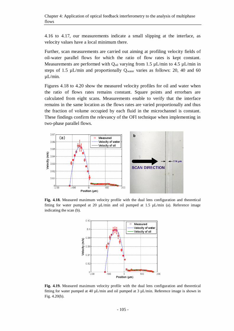
Chapter 4: Application of optical feedback interferometry to the analysis of multiphase
flows
- 105 -
4.16 to 4.17, our measurements indicate a small slipping at the interface, as
velocity values have a local minimum there.
Further, scan measurements are carried out aiming at profiling velocity fields of
oil-water parallel flows for which the ratio of flow rates is kept constant.
Measurements are performed with Qoil varying from 1.5 µL/min to 4.5 µL/min in
steps of 1.5 µL/min and proportionally Qwater varies as follows: 20, 40 and 60
µL/min.
Figures 4.18 to 4.20 show the measured velocity profiles for oil and water when
the ratio of flows rates remains constant. Square points and errorbars are
calculated from eight scans. Measurements enable to verify that the interface
remains in the same location as the flows rates are varied proportionally and thus
the fraction of volume occupied by each fluid in the microchannel is constant.
These findings confirm the relevancy of the OFI technique when implementing in
two-phase parallel flows.
Fig. 4.18. Measured maximum velocity profile with the dual lens configuration and theoretical
fitting for water pumped at 20 µL/min and oil pumped at 1.5 µL/min (a). Reference image
indicating the scan (b).
Fig. 4.19. Measured maximum velocity profile with the dual lens configuration and theoretical
fitting for water pumped at 40 µL/min and oil pumped at 3 µL/min. Reference image is shown in
Fig. 4.20(b).
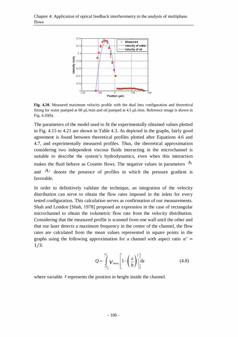
Chapter 4: Application of optical feedback interferometry to the analysis of multiphase
flows
- 106 -
Fig. 4.20. Measured maximum velocity profile with the dual lens configuration and theoretical
fitting for water pumped at 60 µL/min and oil pumped at 4.5 µL/min. Reference image is shown in
Fig. 4.20(b).
The parameters of the model used to fit the experimentally obtained values plotted
in Fig. 4.15 to 4.21 are shown in Table 4.3. As depicted in the graphs, fairly good
agreement is found between theoretical profiles plotted after Equations 4.6 and
4.7, and experimentally measured profiles. Thus, the theoretical approximation
considering two independent viscous fluids interacting in the microchannel is
suitable to describe the system’s hydrodynamics, even when this interaction
makes the fluid behave as Couette flows. The negative values in parameters 1A
and 2A denote the presence of profiles in which the pressure gradient is
favorable.
In order to definitively validate the technique, an integration of the velocity
distribution can serve to obtain the flow rates imposed in the inlets for every
tested configuration. This calculation serves as confirmation of our measurements.
Shah and London [Shah, 1978] proposed an expression in the case of rectangular
microchannel to obtain the volumetric flow rate from the velocity distribution.
Considering that the measured profile is scanned from one wall until the other and
that our laser detects a maximum frequency in the center of the channel, the flow
rates are calculated from the mean values represented in square points in the
graphs using the following approximation for a channel with aspect ratio 𝛼∗ =
1/3:
22
.
2
1 d
h
meash
zQ z
hv
(4.8)
where variable z represents the position in height inside the channel.
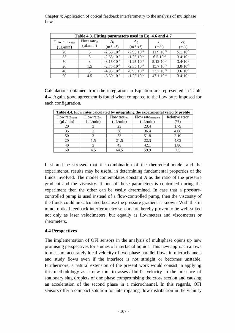
Chapter 4: Application of optical feedback interferometry to the analysis of multiphase
flows
- 107 -
Table 4.3. Fitting parameters used in Eq. 4.6 and 4.7
Flow ratewater
(µL/min)
Flow rateoil
(µL/min) 1A
(m-1·s-1)
2A
(m-1·s-1)
1iv
(m/s)
2iv
(m/s)
20 3 -2.65·10-7 -2.95·10-5 11.9·10-3 5.1·10-3
35 3 -2.65·10-7 -1.25·10-6 6.5·10-3 3.4·10-3
50 3 -3.15·10-7 -1.25·10-6 5.12·10-3 3.4·10-3
20 1.5 -2.75·10-7 -2.35·10-6 15.7·10-3 3.0·10-3
40 3 -4.95·10-7 -6.95·10-6 33.7·10-3 3.6·10-3
60 4.5 -6.60·10-7 -1.25·10-6 47.1·10-3 3.4·10-3
Calculations obtained from the integration in Equation are represented in Table
4.4. Again, good agreement is found when compared to the flow rates imposed for
each configuration.
Table 4.4. Flow rates calculated by integrating the experimental velocity profile
Flow ratewater
(µL/min)
Flow rateoil
(µL/min)
Flow ratetotal
(µL/min)
Flow ratemeasured
(µL/min)
Relative error
(%)
20 3 23 23.4 1.79
35 3 38 36.4 4.08
50 3 53 51.8 2.19
20 1.5 21.5 22.3 4.02
40 3 43 42.1 1.86
60 4.5 64.5 59.9 7.5
It should be stressed that the combination of the theoretical model and the
experimental results may be useful in determining fundamental properties of the
fluids involved. The model contemplates constant A as the ratio of the pressure
gradient and the viscosity. If one of those parameters is controlled during the
experiment then the other can be easily determined. In case that a pressure-
controlled pump is used instead of a flow-controlled pump, then the viscosity of
the fluids could be calculated because the pressure gradient is known. With this in
mind, optical feedback interferometry sensors are hereby proven to be well-suited
not only as laser velocimeters, but equally as flowmeters and viscometers or
rheometers.
4.4 Perspectives
The implementation of OFI sensors in the analysis of multiphase opens up new
promising perspectives for studies of interfacial liquids. This new approach allows
to measure accurately local velocity of two-phase parallel flows in microchannels
and study flows even if the interface is not straight or becomes unstable.
Furthermore, a natural extension of the present work would consist in applying
this methodology as a new tool to assess fluid’s velocity in the presence of
stationary slug droplets of one phase compromising the cross section and causing
an acceleration of the second phase in a microchannel. In this regards, OFI
sensors offer a compact solution for interrogating flow distribution in the vicinity

Chapter 4: Application of optical feedback interferometry to the analysis of multiphase
flows
- 108 -
of interfaces typically found in the studies of slug flows, transport of highly
viscous fluids and organic-water mixtures.
Conclusions
- 109 -
Conclusions
The present thesis had the purpose of implementing the optical feedback
interferometry technique for multiple sensing applications in fluidic systems with
interest in biomedical and chemical engineering and with experimental projection
mainly at the micrometric scale but also with larger channels.
In the first chapter, we reviewed the Doppler methods currently used for flow
quantification. A direct comparison between all the methods highlighted the full
potential of optical feedback interferometry (OFI) sensors in terms of spatial
resolution, costs, ease of mounting and bulkiness. OFI presents a viable
alternative to other Doppler techniques allowing flow measurements and is one of
the few techniques that can address flow measurements at the micro-scale. A
notable ongoing research in the potential of optical feedback systems is actively
being developed in the field, thus pushing the new applications of the emerging
field of optofluidics. The motivations of the present thesis are presented in the
frame of the number of unexplored issues and applications related to OFI and its
implementation for fluid flow assessment in both the single and multiple
scattering regime.
Chapter 2 presents the fundaments of the optical feedback effect in the case of the
interaction of the laser with a group of particles. A discussion on the scattering
regimes that may be applied to the theoretical approaches governing the laser-
Conclusions
- 110 -
fluid interaction is presented. A derivation of the equations explaining the physics
supporting the phenomenon is proposed. The derivation of the rate equations that
constitute the core theory of the lasers subject to external feedback has been
extended to generate a simple model that takes into account the impact of a
plurality of particles contributing to the laser feedback. In addition, we provided a
complete description of the OFI sensor principles that included a set of
characterization measurements of the lasers involved in the experiments presented
in this manuscript.
In Chapter 3, we present the processing methods that could be used to extract the
quantitative values of velocity of flows in a microchannel and presented an
analysis of their suitability to successfully retrieve the quantitative information of
flows in both the single and the multiple scattering regime. We found that the
weighted moment method is well-suited for Doppler frequency shift
determination and velocity calculation as long as the fluid holds a concentration
similar to 4 % of full-cream milk or higher, as demonstrated by the relative errors
below 8 %. In addition, the relative errors obtained for weighted moment
processing method are lower than 6 % for a wide range of flow rates. The second
processing method tested, consisting in using a cutoff frequency method provides
a reasonable accuracy in the measurements at flow rates below 20 ul/min and may
provide an accurate measurement for concentrations up to 4 % of full-cream milk
with relative errors associated below 5 %.
In addition, from the number of elements that we identified as potential research
work in Chapter 1, we have addressed experimentally in Chapter 3 multiple
applications of the optical feedback interferometry in fluid flow sensing. We have
tested the OFI technique and its capabilities for flow measurements in
microchannels, flow profiling, ex-vivo flow mapping, the analysis of non-steady
flows and single particle detection. We demonstrate thereby that OFI is a suitable
technique to be implemented at the microscale for flow sensing with reasonable
accuracy. The demonstrations presented in the third chapter clearly emphasize the
latent fertile ground of possibilities that OFI opens as a new simple optical
technique for milli and microchannel flow sensing, flow steadiness
characterization and particle detection and location in microfluidic devices. The
experimental evidences presented in this chapter present OFI as powerful non-
contact sensing method in the field of optical measurement techniques at the
microscale.
Finally, in the fourth chapter, we present what we believe is the first
implementation of optical feedback interferometry sensors for the analysis of
multiphase flows. We combined the possibilities of flow profiling with an
analytical model issue from the Couette flow approximation, to reconstruct the
velocity profile of immiscible liquids at the microscale. This theoretical model
was developed in this thesis for describing the hydrodynamics of the immiscible
Conclusions
- 111 -
fluids. The model fits fairly well with the experimental measurements and the
methodology presented opens up new possibilities for understanding behavior of
parallel flows and the influence of one flow on the other mostly evidenced by the
slipping at the interface that is equivalent to consider moving plates of Couette
flows under a pressure gradient. This behavior allows us to understand under
which circumstances the velocity profile of the flows is developed independently
and their interaction is minimal.
The work presented in this thesis paves the way to further developments in the
field of optofluidic implementation, microchannel flows interrogation, particle
characterization in microfluidic channels and multiphase flow analysis.
Our group at LAAS-CNRS is currently developing new automated OFI systems
enabling flow profiling at the microscale, which incorporate a micromirror to
guide the laser towards the flow. This avoids using micromechanical stepping
devices to perform the scan during flow profiling and flow mapping
measurements, thus simplifying the scanning scheme of the sensor. An extension
of this system is being investigated for scan cancer detection in the European
project Diagnoptics. The project consists in developing a set of photonic
instrumentation tools including the design and development of an optical feedback
interferometry sensor capable of quantifying the microcirculation associated to
malignant tissue as an indicator of skin cancer, especially the melanomas.
In the field of particle detection in microfluidic devices new research work is
being conducted to implement OFI for the characterization of particles in a flow
beyond the detection and location in a profile. Further work will deal with the
possible discrimination of particles by size and shape using different
methodologies such as continuous signal burst scanning and its relation to the
geometrical properties of the particles. Moreover, to the best of our knowledge, no
OFI sensing has been tested for detecting particles significantly smaller than the
laser wavelength, where Rayleigh scattering rules the interaction. Future
theoretical and experimental work could be directed towards the detection and
characterization of small particles producing extremely weak Rayleigh scattering.
A set of new perspectives are identified to further implement optical feedback
interferometry sensors in other situations involving multiphase flows. In this
regard, OFI can be potentially tested for the analysis of droplets in gas-liquid
flows, by providing information on the velocity and sizes as they pass through the
sensing volume. Other possibilities are found in the analysis of slug flows of
different immiscible fluids in microreactors. Stationary slug flows of one fluidic
phase can compromise the cross section of the channels, and then cause an
acceleration of the second phase that can be quantified with OFI flow profiling
and mapping.

- 112 -
List of publications
- 113 -
List of publications
Conference papers
Quotb, A., Ramírez-Miquet, E. E., Tronche, C. and Perchoux, J. (2014). Optical
feedback interferometry sensor for flow characterization inside ex-vivo vessel.
Proc. IEEE Sensors, 313-316.
Ramírez-Miquet, E. E., Arriaga, A. L., Quotb, A., Sotolongo-Costa, O. and
Perchoux, J. (2015). In-situ measurement of non-steady flows using optical
feedback interferometry. Proc. IEEE International Conference on Industrial
Technology, 1469-1473.
Ramírez-Miquet, E. E., Sotolongo-Costa, O., Quotb, A., Loubière, K., Plat, L. and
Perchoux, J. (2016). Profiling oil-water flows in microchannel: preliminary results
using optical feedback interferometry. Optical Measurement Techniques for
Systems and Structures III, 251-258.
Journal papers
Perchoux, J., Quotb, A., Atashkhooei, R., Azcona, F. J., Ramírez-Miquet, E. E.,
Bernal, O., Jha, A., Luna-Arriaga, A., Yanez, C., Caum, J., Bosch, T. and Royo,
S. (2016). Current developments on optical feedback interferometry as an all-
optical sensor for biomedical applications. Sensors 16, 694.
Ramírez-Miquet, E. E., Perchoux, J., Loubière, K., Tronche, C., Prat, L. and
Sotolongo-Costa, O. (2016). Optical feedback interferometry for velocity
measurement of parallel liquid-liquid flows in a microchannel. Sensors 16, 1233.
References
- 114 -
References
Acket, G., Lenstra, D., Den Boef, A. and Verbeek, B. (1984). The influence of
feedback intensity on longitudinal mode properties and optical noise in index-
guided semiconductor lasers. IEEE J. Quantum Electron. 20(10), 1163-1169.
Açikgöz, M., França, F., Lahey Jr, R. T. (1992). An experimental study of three-
phase flow regime. Int. J. Multiphase Flow 18(3), 327-336.
Ahn Y.C., Jung W. and Chen, Z. (2008). Optical sectioning for microfluidics:
secondary flow and mixing in a meandering microchannel. Lab Chip. 8, 125-133.
Akamatsu, S., Kondo, Y. and Dohi, S. (1996). Velocity measurement with a new
ultrasonic Doppler method independent of angle of incidence. J. Anesth. 10, 133-
139.
Alexandrova, A. and Welsch, C.P. (2016). Laser diode self-mixing technique for
liquid velocimetry. Nucl. Instrum. Meth. A, doi: 10.1016/j.nima.2015.12.042
Atashkhooei, R., Royo, S. and Azcona, F. J. (2013). Dealing with speckle effects
in self-mixing interferometry measurements. IEEE Sensors J., 13(5), 1641-1647.
Atashkhooei, R., Urresty, J. C. Royo, S., Riba, J. R. and Romeral, L. (2014).
Runout tracking in electric motors using self-mixing interferometry. IEEE/ASME
Trans. Mechatron. 19, 184–190.
Attwell, D., Buchan, A.M., Charpak, S., Lauritzen, M., Macvicar, B.A. and
Newman, E.A. (2010). Glial and neuronal control of brain blood flow. Nature
468, 232-243.
Arriaga, A. L., Bony, F. and Bosch, T. (2016). Real-time algorithm for versatile
displacement sensors based on self-mixing interferometry. IEEE Sensors J. 16,
195-202.
References
- 115 -
Arriaga, A. L. (2014a). Analysis and implementation of algorithms for embedded
self-mixing displacement sensors design. Thesis dissertation.
Arriaga, A. L., Bony, F. and Bosch, T. (2014b). Speckle-insensitive fringe
detection method based on Hilbert transform for self-mixing interferometry. App.
Opt. 53(30), 6954-6962.
Baker, D. W. (1970). Pulsed ultrasonic Doppler blood flow sensing. IEEE Trans.
Sonic. Ultrasonics SU 17(3), 170-185.
Baldini, F. (2006). Optical, chemical, and biochemical sensors in medicine. SPIE
Newsroom, doi: 10.1117/2.1200602.0061.
Ball, G. J. (1988). A stochstic model for laser transit velocimeter correlograms in
flows with high vorticity. J. Mod. Opt. 35(5), 761-782.
Bernal, O., D., Zabit, U. and Bosch, T. M. (2015). Robust method of stabilization
of optical feedback regime by using adaptive optics for a self-mixing micro-
interferometer laser displacement sensor. IEEE J. Sel. Top. Quant.
Electron., 21(4), 336-343.
Bes, C., Belloeil, V., Plantier, G., Gourinat, Y. and Bosch, T. (2007). A self-
mixing laser sensor design with an extended Kalman filter for optimal online
structural analysis and damping evaluation. IEEE/ASME Trans. Mechatronics
12(3), 387-394.
Binzoni, T., Torricelli, A., Giust, R., Sanguinetti, B., Bernhard, P. and Spinelli, L.
(2014). Bone tissue phantoms for optical flowmeters at large interoptode spacing
generated by 3D-stereolithography. Biomed. Opt. Express, 5(8), 2715-2725.
Bohren, C. F. and Huffman, D. R. (2004) Absorption and scattering of light by
small particles. Wiley-VCH Verlag GmbH & Co.
Bonner, R. and Nossal, R. (1981). Model for laser Doppler measurements of
blood flow in tissue. Appl. Opt. 20(12), 2097-2107.
Bosch, T., Servagent, N. and Donati, S. (2001) Optical feedback interferometry
for sensing application. Opt. Eng. 40, 20–27.
Boppart, S. A., Luo, W., Marks, D. L. and Singletary, K. W. (2004). Optical
coherence tomography: feasibility for basic research and image-guided surgery of
breast cancer. Breast Cancer Res Treat 84, 85–97.
Brennen, C. E. (2005). Fundamentals of multiphase flows. Cambridge University
Press.
Büttner, L., Skupsch, C., König, J., & Czarske, J. (2010). Optic simulation and
optimization of a laser Doppler velocity profile sensor for microfluidic
applications. Opt. Eng., 49(7), 073602.
Cadel, D. R. and Lowe, K. T. (2015). Cross-correlation Doppler global
velocimetry (CC-DGV). Opt. Lasers Eng. 71, 51-61.
References
- 116 -
Campagnolo, L., Roman, S., Perchoux, J. and Lorthois, S. (2012). A new optical
feedback interferometer for measuring red blood cell velocity distributions in
individual capillaries: a feasibility study in microchannels. Comput. Methods
Biomech. Biomed. Engin. 15(sup1), 104-105.
Campagnolo, L., Nikolić, M., Perchoux, J., Lim, Y. L., Bertling, K., Loubière, K.,
Prat, L., Rakić, A. D. and Bosch, T. (2013a). Flow profile measurement in
microchannel using the optical feedback interferometry sensing technique.
Microfluid. Nanofluid. 14, 113-119.
Campagnolo, L. (2013b). Optical feedback interferometry for flow measurements
in microchannels. Doctoral dissertation.
Chen, Z., Milner, T.E., Srinivas, S., Wang, X., Malekafzali, A., van Gemert, M.
J., Nelson, J.S. (1997). Noninvasive imaging of in vivo blood flow velocity using
optical Doppler tomography. Opt. Lett. 22, 1119-1121.
Clancy, P. S. and Samimy, M. (1997). Two-component planar Doppler
velocimetry in high-speed flows. AIAA J. 35(11), 1729–1738.
Clancy, P., Samimy, M. and Erskine, W. R. (1999). Planar Doppler Velocimetry:
three-component velocimetry in supersonic jets. AIAA J. 37(6), 700–707.
Clifford, P. S., Ella, S. R., Stupica, A. J., Nourian, Z., Li, M., Martinez-Lemus, L.
A., Dora, K. A., Yang Y., Davis M. J., Pohl U., Meininger, G. A. and Hill, M. A.
(2011). Spatial Distribution and Mechanical Function of Elastin in Resistance
Arteries A Role in Bearing Longitudinal Stress. Arteriosclerosis, thrombosis, and
vascular biology, 31(12), 2889-2896.
Davis, M. A., Kazmi, S. M. S. and Dunn, A. K. (2014). Imaging depth and
multiple scattering in laser speckle contrast imaging. J. Biomed. Opt. 19(8),
086001.
de Mul, F. F. M., van Spijker, J., van der Plas, D., Greve, J., Aarnoudse, J. G.,
Smits, T. M. (1984). Mini laser-Doppler (blood) flow monitor with diode laser
source and detection integrated in the probe. Appl. Opt. 23(17), 2970-2973.
de Mul, F. F. M., Koelink, M. H., Weijers, A. L., Greve, J., Aarnoudse, J.G.,
Graaff, R. and Dassel, A. C. M. (1992). Self-mixing laser Doppler velocimetry of
liquid flow and of blood perfusion in tissue. Appl. Opt. 31(27), 5844-5851.
de Mul, F. F. M., Koelink, M.H., Weijers, A.L., Greve, J., Aarnoudse, J.G.,
Graaff, R. and Dassel, A.C.M. (1993) A semiconductor laser used for direct
measurement of the blood perfusion of tissue. IEEE Trans. Biomed. Eng. 40(2),
208-210.
Donati, S. (1978). Laser interferometry by induced modulation of cavity field. J.
Appl. Phys. 49(2), 495-497.
Donati, S. (2000). Photodetectors, Devices, Circuits and Applications, Chapter 8,
Prentice Hall, Upper Saddle River, NJ.
References
- 117 -
Donati, S. (2012). Developing self-mixing interferometry for instrumentation and
measurements. Laser Photonics Rev. 6(3), 393-417.
Donati, S., and Norgia, M. (2014). Self-mixing interferometry for biomedical
signals sensing. IEEE J. Sel. Top. Quant. 20(2), 104-111.
Doppler, C. (1843). Über das farbige Licht der Doppelsterne und eineger anderer
Gestirne des Himmels. Abhandl Konigl Bohm Ges. Ser. 2, 465-482.
Drexel, W. (2004). Ultrahigh resolution optical coherence tomography. J.
Biomed. Opt. 9(1), 47-74.
Elliott, G.S., Samimy, M. and Arnette, S. A. (1992). Study of compressible
mixing layers using filtered Rayleigh scattering based visualizations,” AIAA J.
30, 2567-2569.
Elliott, G. S., Samimy, M., and Arnette, S. A. (1994). A molecular filter based
diagnostics in high-speed flows. Exp. Fluids 18, 107-118.
Elliott, G. S. and Beutner T. J. (1999). Molecular Filter based planar Doppler
velocimetry. Prog. Aeros. Sci. 35, 799-845.
Fainman, Y., Lee, L., Psaltis, D., and Yang, C. (2009). Optofluidics:
fundamentals, devices, and applications. McGraw-Hill, Inc.
Figueiras, E., Oliveira, R., Lourenço, C. F., Campos, R., Humeau-Heurtier, A.,
Barbosa, R. M., Laranjinha, J., Ferreira, L. F. R. and de Mul, F. F. M. (2013).
Self-mixing microprobe for monitoring microvascular perfusion in rat brain. Med.
Biol. Eng. Comput. 51(1-2), 103-112.
Fischer, A., Wilke, U., Schlüßler, R., Haufe, D., Sandner, T and Czarske, J.
(2014). Extension of frequency modulated Doppler global velocimetry for the
investigation of unsteady spray flows. Opt. Lasers Eng. 63, 1-10.
Foreman Jr., J. W. George, E. W. and Lewis, R. D. (1965). Measurement of
localized velocities in gases with a laser Doppler flowmeter. Appl. Phys. Lett.
7(4), 77-78.
Foreman, J. W., George, E. W., Jetton, J. L., Lewis, R. D., Thornton, J. R. and
Watson, H. J. (1966). 8C2-fluid flow measurements with a laser Doppler
velocimeter. IEEE J. Quant. Electron. 2(8), 260-266.
Foroughi, H. and Kawaji, M. (2011). Viscous oil–water flows in a microchannel
initially saturated with oil: flow patterns and pressure drop characteristics. Int. J.
Multiphas. Flow, 37(9), 1147-1155.
Förster, W., Karpinsky, G., Krain, H., Röhle, I. and Schodl, R. (2002). 3-
Component Doppler laser-two-focus velocimetry applied to a transonic
centrifugal compressor. Laser Techniques for Fluid Mechanics, 55-74.
Franklin, D. L., Schelegel, W. and Rushmer, R. F. (1959). Blood flow measured
by Doppler Frequency shift of back scattered ultrasound. Science 134, 564-565.
References
- 118 -
FritzGerard, D. E. and Drumm, J. E. (1977). Noninvasive measurement of the
fetal circulation using ultrasound: a new method. Br. Med. J. 2, 637-641.
Giuliani, G., M. Norgia, M., S. Donati, S. and T. Bosch, T. (2002). Laser diode
self-mixing technique for sensing applications. J. Opt. A: Pure Appl. Opt. 4,
S283–S294.
Goldman, L. (1981). The biomedical laser: technology and clinical applications.
Chapter 13.
Gordon, A., & Vynnycky, M. (2014). Analysis of Two-Phase Flow in the Gas
Diffusion Layer of a Polymer Electrolyte Fuel Cell. In Progress in Industrial
Mathematics at ECMI 2012. Springer International Publishing, 177-183.
Harris, S. J. and Maricq, M. M. (2001). Signature size distributions for diesel and
gasoline engine exhaust particulate matter. J. Aerosol Sci., 32(6), 749-764.
Hilsum, C. and King, P. G. R. (1963). Some demonstrations of the properties of
optical masers. Contemp. Phys. 4, 435-444.
Honeycutt, T. E. and Otto, W. (1972). FM-CW radar range measurement with a
CO2 laser. IEEE J. Quantum Electron. 8, 91-92.
Huang, D., Swanson, E. A., Lin, C. P., Schuman, J. S., Stinson, W. G., Chang,
W., Hee, M. R., Flotte, T., Gregory, K., Puliafito, C. A. and Fujimoto, J. M.
(1991). Optical coherence tomography. Science 254, 1178-1181.
Jones, T. B. (2001). Development and Testing of the Virginia Tech Doppler
Global Velocimeter (DGV). MSc. Thesis, p. 104.
Kalkman, J., Bykov, A. V., Streekstra, G. J. and van Leeuwen, T. G. (2012).
Multiple scattering effects in Doppler optical coherence tomography of flowing
blood. Phys. Med. Biol. 57, 1907-1917.
Kamishima, T. and Quayle, J. M. (2013). Small Vessel Myography. In Essential
Guide to Reading Biomedical Papers: Recognising and Interpreting Best Practice.
Wiley-Blackwell, 39-48.
Kane, D. M. and Shore, K. A. (Eds.) “Unlocking Dynamical Diversity - Optical
feedback effects on semiconductor lasers”, Wiley, 2005.
Kashid, M. N., Rivas, D. F., Agar, D. W. and Turek, S. (2008). On the
hydrodynamics of liquid–liquid slug flow capillary microreactors. Asia-Pac. J.
Chem. Eng. 3(2), 151-160.
Kim, G and Menon, R. (2014). An ultra-small 3D computational microscope.
Appl. Phys. Lett. 105, 061114.
King, P. G. R. and Steward, G. J. (1963). Metrology with an optical maser. New
Sci. 17, 180-182.
King, P. G. R. and Steward, G. J. (1968). Apparatus for measurement of lengths
and of other physical parameters which are capable of altering an optical path
length. U.S. patent 3409370.
References
- 119 -
Kliese, R., Taimre, T., Bakar, A. A. A., Lim, Y. L., Bertling, K., Nikolić, M.,
Perchoux, J., Bosch, T. and Rakić, A. D. (2014). Solving self-mixing equations
for arbitrary feedback levels: a concise algorithm. Appl. Opt. 53(1), 3723-3736.
Kliese, R., Lim, Y. L., Bosch, T. and Rakić, A. D. (2010). GaN laser self-mixing
velocimeter for measuring slow flows. Opt. Lett. 35(6), 814-816.
Koelink, M. H., Slot, M., de Mul, F. F. M., Greve, J., Graaff, R., Dassel, A. C. M.
and Aarnoudse, J.G. (1992). Laser Doppler velocimeter based on the self-mixing
effect in a fiber-coupled semiconductor laser: theory. Appl. Opt. 31(18), 3401-
3408.
Komine, H. and Brosnan, S. (1991). Instantaneous, three-component, Doppler
global velocimetry. Laser Anemom. 1, 273-277.
König, J., Voigt, A., Büttner L. and Czarske J. (2010). Precise micro flow rate
measurements by a laser Doppler velocity profile sensor with time division
multiplexing. Meas. Sci. Technol. 21, 074005.
Kost, F. and Kapteijn, C. (1997). Application of Laser-Two-Focus Velocimetry to
Transonic Turbine Flows. 7th International Conference on Laser Anemometry -
Advances and Applications, University of Karlsruhe, Germany, September 8-11.
Kumara, W. A. S., Elseth, G., Halvorsen, B. M. and Melaaen, M. C. (2010).
Comparison of Particle Image Velocimetry and Laser Doppler Anemometry
measurement methods applied to the oil-water flow in horizontal pipe. Flow
Meas. Instrum. 21, 105-117.
Lang, R. and Kobayashi, K. (1980). External optical feedback effects on
semiconductor injection laser properties. IEEE J. Quantum Electron. QE-16, 347-
355.
Langlois, W. E. and Deville, M. O. (2014). Exact Solutions to the Equations of
Viscous Flow. In Slow Viscous Flow, pp. 105-143.
Leitgeb, R. A., Werkmeister, R. M., Blatter, C. and Schmetterer, L. (2014).
Doppler optical coherence tomography. Prog. Ret. Eye Res. 41, 26-43.
Liu, J., Cai, B., Zhu, J., Ding, G., Zhao, X., Yang, C. and Chen, D. (2004).
Process research of high aspect ratio microstructure using SU-8 resist. Microsyst.
Tech. 10, 265-268.
Lim, Y. L., Kliese, K., Bertling, K., Tanimizu, K., Jacobs, P. A. and Aleksandar
D. Rakić, A. (2010) Self-mixing flow sensor using a monolithic VCSEL array
with parallel readout. Opt. Express 18(11), 11720-11727.
Lohwasser, R. and Soelkner, G. (1999). Experimental and theoretical laser-
Doppler frequency spectra of a tissuelike model of a human head with capillaries.
Applied optics, 38(10), 2128-2137.
References
- 120 -
Lu, X. and Kassab, G. S. (2011). Assessment of endothelial function of large,
medium, and small vessels: a unified myograph. Am. J. Physiol. Heart Circ.
Physiol. 300(1), H94-H100.
Maret, G. and Wolf, P. E. (1987). multiple light scattering from disordered media.
The effect of brownian motion of scatterers. Z. Phys. B Cond. Matter 65, 409-413.
Merlo, S. and Donati, S. (1997). IEEE J. Quantum Electron. 33(4), 527–531.
McCallum, W. D., Olson, R. F., Daigle, R. E. and Baker, D. W. (1977). Real time
analysis of Doppler signals obtained from the fetoplacental circulation.
Ultrasound. Med. 3B, 1361-1364.
McCarron, J. G., Crichton, C. A., Langton, P. D., MacKenzie, A. and Smith, G. L.
(1997). Myogenic contraction by modulation of voltage-dependent calcium
currents in isolated rat cerebral arteries. J. Physiol., 498(Pt 2), 371-379.
McKenzie, R. L. (1996). Measurement capabilities of planar Doppler velocimetry
using pulsed lasers. Appl. Opt. 35(6), 948-964.
McKenzie, R.L. (1997). Planar Doppler velocimetry performance in low-speed
flows. AIAA Paper 97-0498.
Menn, N. (2004). Practical Optics. Elsevier Academic Press.
Meyers, J. F. (1992). Doppler Global Velocimetry: The Next Generation? AIAA
17th Aerospace Ground Testing Conference.
Michalski, M. -C., Briarn, V. and Michel, F. (2001). Optical parameters of milk
fat globules for laser light scattering measurements. Lait 81, 787-796.
Miles, R. and Lempert, W. (1990). Two-dimensional measurement of density,
velocity, and temperature of turbulent air flows from UV Rayleigh scattering.
Appl. Phys. B B51, 1-7.
Mishchenko, M. I., Hovenier, J. W. and Mackowski, D. W. (2004). Single
scattering by a small volume element. J. Opt. Soc. Am. 21(1), 71-87.
Moger, J., Matcher, S. J., Winlove, C. P., & Shore, A. (2005). The effect of
multiple scattering on velocity profiles measured using Doppler OCT. J. Phys.D:
Appl. Phys. 38(15), 2597-2605.
Mowla, A., Nikolić, M., Taimre, T., Tucker, J. R., Lim, Y. L., Bertling, K. and
Rakić, A. D. (2015). Effect of the optical system on the Doppler spectrum in
laser-feedback interferometry. Appl. Opt. 54(1), 18-26.
Murakawa, H., Muramatsu, E., Sugimoto, K., Takenaka, N., & Furuichi, N.
(2015). A dealiasing method for use with ultrasonic pulsed Doppler in measuring
velocity profiles and flow rates in pipes. Meas. Sci. Technol. 26(8), 085301.
Nakamura, T., Hayashi, K., Taenaka, Y., Umezu, M., Nakatani, T. and Takano, H.
(1986). Ultrasonic flowmeter with implentable miniature sensors. Med. Biol. Eng.
Comput. 24, 235-242.
References
- 121 -
Nemani, K. V., Moodie, K. L., Brennick, J. B., Su, A. and Gimi, B. (2013). In
vitro and in vivo evaluation of SU-8 biocompatibility. Mat. Sci. Eng. C 33, 4453-
4459.
Nikolić, M., Hicks, E., Lim, Y. L., Bertling, K. and Rakić, A. D. (2013). Self-
mixing laser Doppler flow sensor: an optofluidic implementation. Appl. Opt.
52(33), 8128-8133.
Nikolić, M., Taimre, T., Tucker, J. R., Lim, Y. L., Bertling, K. and Rakić (2014).
Laser dynamics under frequency-shifted optical feedback with random phase.
Electron. Lett. 50(19), 1380-1382.
Nikolić, M., Lim, Y. L., Bertling, K., Taimre, T. and Rakić, A. D. (2015).
Multiple signal classification for self-mixing flowmetry. Appl. Opt. 54(9), 2193-
2198
Nilsson, G. E. (1984). Signal processor for laser Doppler tissue flowmeters. Med.
Biol. Eng. Comput. 22, 343-348.
Norgia, M., Pesatori, A. and Rovati, L. (2010). Low-cost optical flowmeter with
analog front-end electronics for blood extracorporeal circulators. IEEE Trans.
Instrum. Meas. 59(5), 1233-1239.
Norgia, M., Pesatori, A. and Rovati, L. (2012). Self-mixing laser Doppler spectra
of extracorporeal blood flow: a theoretical and experimental study. IEEE Sensors
J. 12(3), 552-557.
Norgia, M., Magnani, A., Melchionni, D. and Pesatori, A. (2015). Drop
measurement system for biomedical application. IEEE Trans. Instrum. Meas.
64(9), 2113-2117.
Norgia, M., Pesatori, A. and Donati, S. (2016). Compact Laser-Diode Instrument
for Flow Measurement. IEEE Trans. Instrum. Meas. 65(6), 1478-1483.
Oddie, G., Shi, H., Durlofsky, L. J., Aziz, K., Pfeffer, B., Holmes, J. A. (2003).
Experimental study of two and three phase flows in large diameter inclined pipes.
Int. J. Multiphase Flow 29, 527-558.
Ortalano, D. M., Picraux, L., Clapp, L., Merchak, P. A. and Schwarts, R. J.
(2015). Pigment dispersion and printing inks with improved coloristic properties.
Patent Application Publication US 2015/0252201 A1.
Osiac, E., Săftoiu, A., Gheonea, D. I., Mandrila, I. and Angelescu, R. (2011).
Optical coherence tomography and Doppler optical coherence tomography in the
gastrointestinal tract. World J. Gastroenterol. 17(1), 15-20.
Parida, O. P. and Bhat, N. (2009). Characterization of optical properties of SU-8
and fabrication of optical components. In Proceedings of the ICOP 2009-
International Conference on Optics and Photonics, Chandigarh, India.
References
- 122 -
Penner, S. S., Davidor, W. and Bien F. (1970). Determination of Interference
Patterns from Laser Produced Schlieren Interferometry. Am. J. Phys. 38(12),
1413-1415.
Perchoux, J., Quotb, A., Atashkhooei, R., Azcona, F. J., Ramírez-Miquet, E. E.,
Bernal, O., Jha, A., Luna-Arriaga, A., Yanez, C., Caum, J., Bosch, T. and Royo,
S. (2016). Current developments on optical feedback interferometry as an all-
optical sensor for biomedical applications. Sensors 16, 694.
Peronneau P. A. and Leger, F. (1969). Doppler ultrasonic pulsed blood flowmeter.
Proc. of the 8th Conference on Medical and Biological Engineering, 10-11.
Petermann, K. (1991). Laser diode modulation and noise. Kluwer Academic
Publishers. Tokyo.
Pohar, A., Lakner, M. and Plazl, I. (2012). Parallel flow of immiscible liquids in a
microreactor: modeling and experimental study. Microfluid. Nanofluid. 12(1-4),
307-316.
Psaltis, D., Quake, S. R. and Yang, C. (2007). Developing optofluidic technology
through the fusion of microfluidics and optics. Nature 442, 381-386.
Quirantes, A., Arroyo, F., & Quirantes-Ros, J. (2001). Multiple light scattering by
spherical particle systems and its dependence on concentration: a T-matrix
study. J. Colloid Interface Sci., 240(1), 78-82.
Quotb, A., Ramírez-Miquet, E. E., Tronche, C. and Perchoux, J. (2014). Optical
feedback interferometry sensor for flow characterization inside ex-vivo vessel. In
IEEE Sensors, 362-365.
Raghunathan, R., Singh, M., Mary E. Dickinson, M. E. and Larin, K. V. (2016).
Optical coherence tomography for embryonic imaging: a review. J. Biomed. Opt.
21(5), 050902.
Raimondi, N. D. M., Prat, L., Gourdon, C. and Tasselli, J. (2014). Experiments of
mass transfer with liquid–liquid slug flow in square microchannels. Chem. Eng.
Sci. 105, 169-178.
Rajadhyaksha, M., Anderson, R. R. and Webb, R. H. (1999). Video-rate confocal
scanning laser microscope for imaging human tissues in vivo. Appl. Opt. 38,
2105-2015.
Ramírez-Miquet, E. E., Arriaga, A. L., Quotb, A., Sotolongo-Costa, O. and
Perchoux, J. (2015). In-situ measurement of non-steady flows using optical
feedback interferometry. In IEEE International Conference on Industrial
Technology, 1469-1473.
Ramírez-Miquet, E. E., Sotolongo-Costa, O., Quotb, A., Loubière, K., Prat. L. and
Perchoux, J. (2016a). Profiling oil-water flows in microchannel: preliminary
results using optical feedback interferometry. Optical measurement techniques for
systems and structures III, 251-258. Shaker Publishing.
References
- 123 -
Ramírez-Miquet, E. E., Perchoux, J., Loubière, K., Tronche, C., Prat, L. and
Sotolongo-Costa, O. (2016b). Optical feedback interferometry for velocity
measurement of parallel liquid-liquid flows in a microchannel. Sensors 16, 1233.
Riva, C., Ross, B. and Benedek, G. B. (1972). Laser Doppler measurements of
blood flow in capillary tubes and retinal arteries.
Invest. Ophthalmol. Vis. Sci. 11(11), 936-944.
Roehle, I. (1998). Method for measuring flow vectors in gas flows
US Patent 5751410 A.
Roehle, I, Karpinski, G. and Schodl, R. (1999). 3-Component-Doppler-Laser-2-
Focus: A new kind of three component velocimeter. 18th International Congress
on Instrumentation in Aerospace Simulation Facilities ICIASF99, Toulouse, 13/1-
13/9.
Roman, S., Lorthois, S., Duru, P. and Risso, F. (2012). Velocimetry of red blood
cells in microvessels by the dual-slit method: Effect of velocity gradients.
Microvasc. Res. 84, 249-261.
Rooze, J., André, M., van der Gulik, G. J. S., Fernández-Rivas, D., Gardeniers, J.
G., Rebrov, E. V., Schouten, J. C. and Keurentjes, J. T. (2012). Hydrodynamic
cavitation in micro channels with channel sizes of 100 and 750 micrometers.
Microfluid. Nanofluid. 12(1-4), 499-508.
Rovati, L., Cattini, S. and Palanisamy, N. (2011). Measurement of the fluid
velocity profile using a self-mixing superluminescent diode. Meas. Sci. Tech.
22(2), 025402.
Rudd, M. (1968). A laser Doppler velocimeter employing the laser as a mixer-
oscillator. J. Sci. Instrum. 1, 723-726.
Rudd, M. J. (1969). A new theoretical model for the laser dopplermeter. J. Phys. E
Scient. Instrum. 2(1), 55-58.
Rudyak, V and Minakov, A. (2014). Modeling and optimization of Y-type
micromixers. Micromachines, 5(4), 886-912.
Salazar-Miranda, D., Castillón, F. F., Sánchez-Sánchez, J. J., Angel-Valenzuela, J.
L., Márquez, H. (2010). Refractive index modulation of su-8 polymer optical
waveguides by means of hybrid photothermal process. Rev. Mex. Ing. Quim. 9(1),
85-90.
Samimy, M. and Wernet, M. P. (2000). Review of planar multiple-component
velocimetry in high-speed flows. AIAA J. 38(4), 553-574.
Satomura, S., (1957). Ultrasonic Doppler method for the inspection of cardiac
functions. J. Acoust. Soc. Am. 29, 1181-1183.
Satomura, S. and Kaneko, Z. (1960). Ultrasonic blood rheograph. Proc. of the 3rd
International Conference on Medical Electronics. London, 254-258.
References
- 124 -
Schodl, R. (1980). A Laser-Iwo-Focus (L2F) velocimeter for automatic flow
vector measurements in the rotating components of turbomachines. J. Fluid Eng.-
T. ASME, 102(4), 412-419.
Seko, A., Mitsuhashi, Y., Morikawa, T., Shimada, J. and Sakurai, K. (1975). Self‐quenching in semiconductor lasers and its applications in optical memory readout.
Appl. Phys. Lett. 27(3), 140-141.
Servagent, N., Mourat, G., Gouaux, F. and Bosch, T. (1998). Analysis of some
intrinsic limitations of a laser range finder using self-mixing interference. Proc. of
3479, 76-83.
Shah, R. K. and London, A. L. (1978). Laminar flow forced convection in ducts: a
source book for compact heat exchanger analytical data (vol. 1). Academic Press.
Shet, A. S. (2008). Characterizing blood microparticles: technical aspects and
challenges. Vasc Health Risk Manag 2008:4(4) 769–774.
Shinohara, S., Mochizuki, A., Yoshida, H. and Sumi, M. (1986). Laser Doppler
velocimeter using the self-mixing effect of a semiconductor laser diode,” Appl.
Opt. 25(9), 1417-1419.
Soares, R. R., Barbosa, H. C., Braga, R. A., Botega J. V. L. and Horgan, G. W.
(2013). Biospeckle PIV (Particle Image Velocimetry) for analyzing fluid flow.
Flow Meas. Instrum. 30, 90–98.
Stern, L., Bakal, A., Tzur, M., Veinguer, M., Mazurski, N., Cohen, N. and Levy,
U. (2014). Doppler-Based Flow Rate Sensing in Microfluidic Channels. Sensors,
14(9), 16799-16807.
Strandness, D. E., Schultz, R. D., Sumner, D. S., Rushmer, R. F. (1967).
Ultrasonic flow detection – a useful technique in the evaluation of peripheral
vascular disease. Am. J. Surg. 113, 311-314.
Sudo, S. Miyasaka, Y., Nemoto, K. Kamikariya, K. and Otsuka, K. (2007).
Detection of small particles in fluid flow using a self-mixing laser. Opt. Express
15(13), 8135-8145.
Sun, J. G., Adie, S. G., Chaney, E. J., Boppart, S. A. (2013). Segmentation and
correlation of optical coherence tomography and x-ray images for breast cancer
diagnostics. J. Innov. Opt. Health Sci. 6(2), 1350015.
Swanson, E. A., Izatt, J. A., Hee, M. R., Huang, D., Lin, C. P. Schuman, J. S.,
Puliafito, C. A. and Fujimoto, J. G. (1993). In-vivo retinal imaging by optical
coherence tomography. Opt. Lett. 18, 1864-1866.
Taimre, T., Nikolić, M., Bertling, K., Lim, Y. L., Bosch, T., Rakić, A. D. (2015).
Adv Opt. Photonics 7, 570-631.
Taitel, Y., Barnea, D. and Brill, J. P. (1995). Stratified three-phase flows in pipes.
Int. J. Multiphase Flow. 21(1), 53-60.
References
- 125 -
Takeda, Y. (1986). Velocity profile measurement by ultrasound Doppler shift
method. Velocity profile measurement by ultrasound Doppler shift method. Int. J.
Heat Fluid Flow 7(4), 313-318
Takeda, Y. (1999). Ultrasonic Doppler method for velocity profile measurement
in fluid dynamics and fluid engineering. Exp. Fluids 26, 177-178.
Tamura, T. and Fronek, A. (1988). New method for Doppler probe angle
determination. J. Biomed. Eng. 10, 271-274.
Tamura, T., Yoganathan, A and Sahn, D. J. (1987). In vitro methods for studying
the accuracy of velocity determination and spatial resolution of a color Doppler
flow mapping system. Am. Heart J. 114, 152-158.
Tamura, T. and Johnston, K. W. (1990). Determination of 2-D velocity vectors
using color Doppler ultrasound. IEEE Ultrasonics 1537-1540.
Thompson, D.H. (1968). A tracer particle fluid velocity meter incorporating a
laser. J. Phys. E 1, 929–932.
Turgeon, M. L. (2004). Clinical Hematology: Theory and Procedures. Chapter 6.
Lippincott Williams & Wilkins.
Vinegar, H. J. and Wellington, S. L. (1987). Tomographic imaging of three-phase
flow experiments. Rev. Scientif. Instrum. 58(1), 96-107.
Voigt, A., Bayer, C., Shirai, K., Büttner L. and Jürgen C. (2008). Laser Doppler
field sensor for high resolution flow velocity imaging without camera. Appl. Opt.
47(27), 5028-5040.
Wang, C. P. (1974). Doppler velocimeter using diffraction grating and white light.
Appl. Opt. 13(5), 1193-1195.
Wang, C. P. (1988). Laser Doppler velocimetry. J. Quant. Spectrosc. Radiat.
Transfer 40(3), 309-319.
Wang, Y., Fawzi, A., Tan, O., Gil-Flamer, J., Huang, D. (2009). Retinal blood
flow detection in diabetic patients by Doppler Fourier domain optical coherence
tomography. Opt. Express 17, 4061-4073.
Wang, Y., Fawzi, A.A., Varma, R., Sadun, A.A., Zhang, X., Tan, O., Izatt, J.A.,
Huang, D. (2011). Pilot study of optical coherence tomography measurement of
retinal blood flow in retinal and optic nerve diseases. Investig. Ophthalmol. Vis.
Sci. 52, 840-845.
Wells, P. N. T. (1969). A range-gated ultrasonic Doppler system. Med. Biol. Eng.
7, 641-652.
Wereley, S. T. and Meinhart, C. D. (2010). Recent advances in micro-particle
image velocimetry. Annu. Rev. Fluid Mech. 42, 557-576.
White, F. M. (1999). Fluid Mechanics, 4th Edition, WBC/Mc Graw-Hill, Boston.
References
- 126 -
Wilkes, J. O. (2006). Fluid Mechanics for Chemical Engineers with Microfluidics
and CFD. Pearson Education.
Wu, L. (2004) Simultaneous measurement of flow velocity and Doppler angle by
the use of Doppler optical coherence tomography. Opt. Lasers Eng. 42, 303-313.
Wu, J. and Gu, M. (2011). Microfluidic sensing: state of the art fabrication and
detection techniques. J. Biomed. Opt. 16(8), 080901.
Yeh, Y. and Cummins, H. Z. (1964) Localized fluid flow measurements with an
He-Ne spectrometer. Appl. Phys. Lett. 4, 176-178.
Yue, J., Rebrow, E. V. and Schouten, J. C. (2014). Gas–liquid–liquid three-phase
flow pattern and pressure drop in a microfluidic chip: similarities with gas–
liquid/liquid–liquid flows. Lab Chip 14, 1632–1649.
Zabit, U. (2010). Optimisation of a self-mixing laser displacement sensor. Thesis
dissertation.
Zakian, C., Dickinson, M and King, T. (2005). Particle sizing and flow
measurement using self-mixing interferometry with a laser diode. J. Opt. A: Pure
Appl. Opt. 7, S445-S452.

Annexes
- 127 -
Annexes
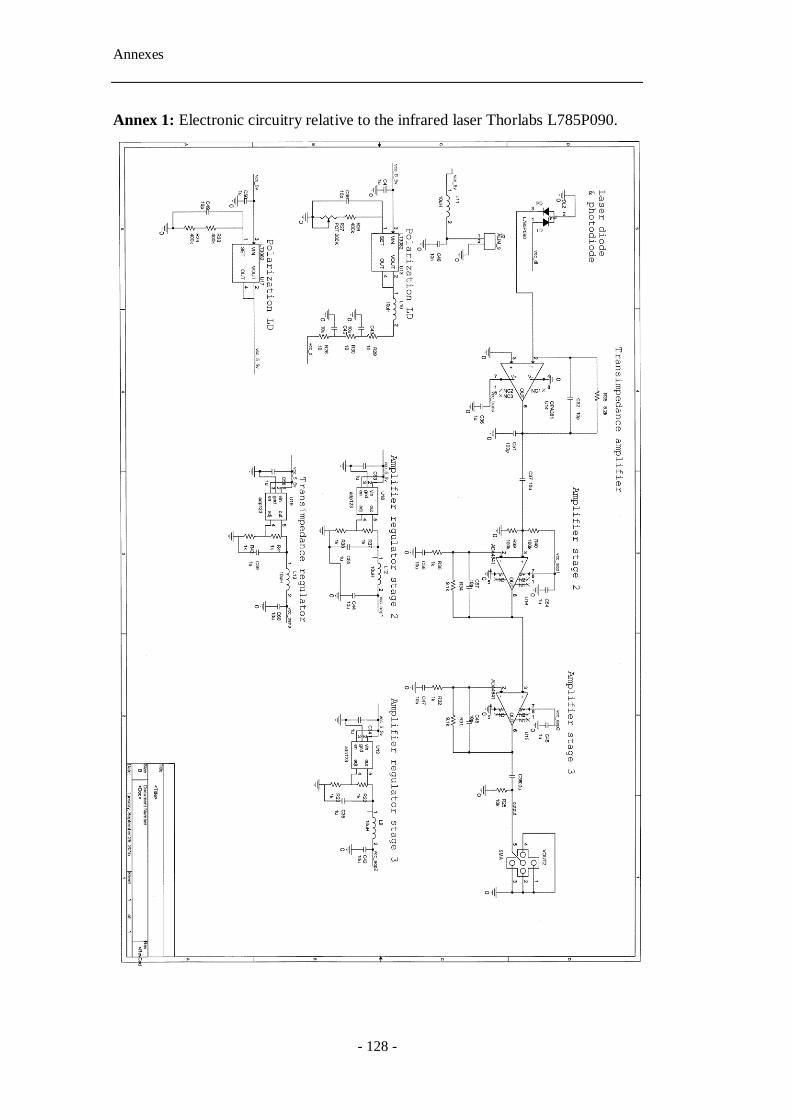
Annexes
- 128 -
Annex 1: Electronic circuitry relative to the infrared laser Thorlabs L785P090.
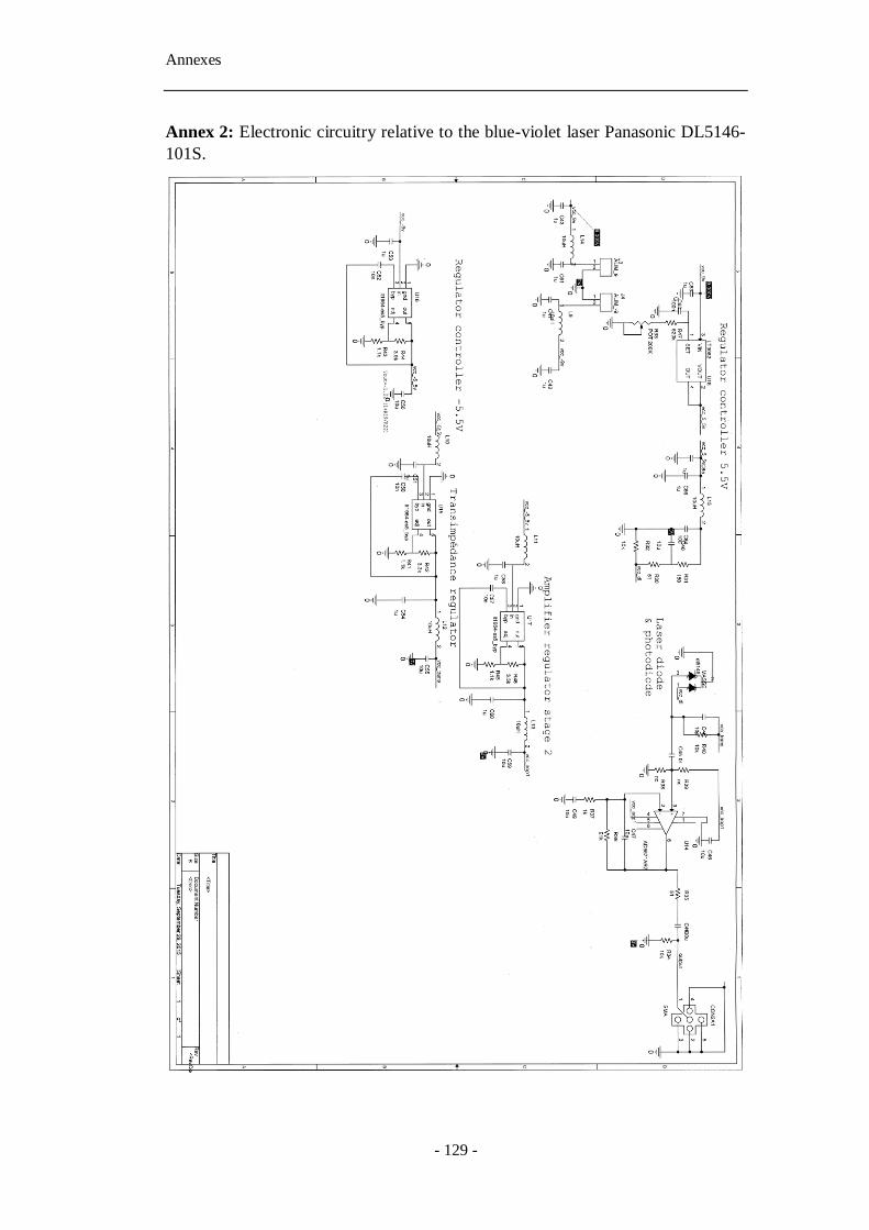
Annexes
- 129 -
Annex 2: Electronic circuitry relative to the blue-violet laser Panasonic DL5146-
101S.