HYPERGRAPH BASED VISUAL CATEGORIZATION
AND SEGMENTATION
BY YUCHI HUANG
A dissertation submitted to the
Graduate School—New Brunswick
Rutgers, The State University of New Jersey
in partial fulfillment of the requirements
for the degree of
Doctor of Philosophy
Graduate Program in Computer Science
Written under the direction of
Professor Dimitris N. Metaxas
and approved by
New Brunswick, New Jersey
October, 2010

ABSTRACT OF THE DISSERTATION
Hypergraph Based Visual Categorization and
Segmentation
by Yuchi Huang
Dissertation Director: Professor Dimitris N. Metaxas
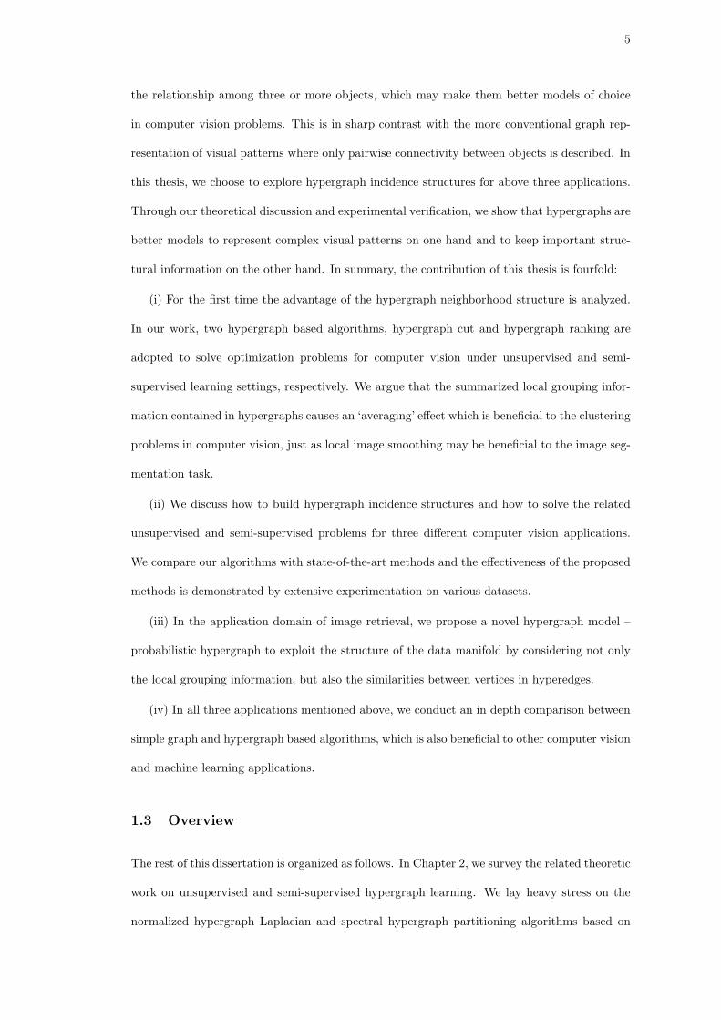
This dissertation explores original techniques for the construction of hypergraph models for
computer vision applications. A hypergraph is a generalization of a pairwise simple graph,
where an edge can connect any number of vertices. The expressive power of the hypergraph
models places a special emphasis on the relationship among three or more objects, which has
made hypergraphs better models of choice in a lot of problems. This is in sharp contrast with
the more conventional graph representation of visual patterns where only pairwise connectivity
between objects is described. The contribution of this thesis is fourfold:
(i) For the first time the advantage of the hypergraph neighborhood structure is analyzed.
We argue that the summarized local grouping information contained in hypergraphs causes an
‘averaging’ effect which is beneficial to the clustering problems, just as local image smoothing
may be beneficial to the image segmentation task.
(ii) We discuss how to build hypergraph incidence structures and how to solve the re-
lated unsupervised and semi-supervised problems for three different computer vision scenarios:
video object segmentation, unsupervised image categorization and image retrieval. We compare
our algorithms with state-of-the-art methods and the effectiveness of the proposed methods is
demonstrated by extensive experimentation on various datasets.
ii

(iii) For the application of image retrieval, we propose a novel hypergraph model — prob-
abilistic hypergraph to exploit the structure of the data manifold by considering not only the
local grouping information, but also the similarities between vertices in hyperedges.
(iv) In all three applications mentioned above, we conduct an in depth comparison between
simple graph and hypergraph based algorithms, which is also beneficial to other computer vision
applications.
iii

Acknowledgements
I would like to express the deepest appreciation to my advisor, Professor Dimitris N. Metaxas,
for his encouragement, guidance and support from the initial to the final level enabled me to
develop an understanding of the subject. He has always directed me toward the interesting areas
in our field, yet still given me great freedom to pursue independent work. He continually and
convincingly conveyed a spirit of adventure and an excitement in regard to research. Without
his guidance and persistent help this dissertation would not have been possible.
I want to thank Dr. Qingshan Liu, who has been working closely with me and contributed
numerous ideas and insights to my research work.
I also thank my thesis committee members, Professor Ahmed Elgammal, Professor Vladimir
Pavlovic, Professor Chandra Kambhamettu for their valuable suggestions regarding my research
and writing of my dissertation. It is an honor for me to have each of them serve in my commit-
tees.
Last but not least, special thanks should be given to my colleagues, all the faculties and the
staff members from CBIM (the Center for Computational Biomedicine Imaging and Modeling)
and the Computer Science Department.
iv

Dedication
This dissertation is dedicated to my parents: Zonggui Huang and Mingfang Yu.
v

Table of Contents
Abstract . . . . . . . . . . . . . . . . . . . . . . . . . . . . . . . . . . . . . . . . . . . . ii
Acknowledgements . . . . . . . . . . . . . . . . . . . . . . . . . . . . . . . . . . . . . iv
Dedication . . . . . . . . . . . . . . . . . . . . . . . . . . . . . . . . . . . . . . . . . . . v
List of Tables . . . . . . . . . . . . . . . . . . . . . . . . . . . . . . . . . . . . . . . . . . ix
List of Figures . . . . . . . . . . . . . . . . . . . . . . . . . . . . . . . . . . . . . . . . . x
1. Introduction . . . . . . . . . . . . . . . . . . . . . . . . . . . . . . . . . . . . . . . . 1
1.1. Motivation: Why Hypergraphs . . . . . . . . . . . . . . . . . . . . . . . . . . . . 1
1.2. Contributions . . . . . . . . . . . . . . . . . . . . . . . . . . . . . . . . . . . . . . 4
1.3. Overview . . . . . . . . . . . . . . . . . . . . . . . . . . . . . . . . . . . . . . . . 5
2. Unsupervised and Semi-Supervised Learning with Hypergraphs . . . . . . . 8
2.1. Previous Work . . . . . . . . . . . . . . . . . . . . . . . . . . . . . . . . . . . . . 8
2.2. Notation and Terminology . . . . . . . . . . . . . . . . . . . . . . . . . . . . . . . 10
2.3. Hypergraph Learning Algorithms . . . . . . . . . . . . . . . . . . . . . . . . . . . 12
2.3.1. Star Expansion . . . . . . . . . . . . . . . . . . . . . . . . . . . . . . . . . 12
2.3.2. Clique Expansion . . . . . . . . . . . . . . . . . . . . . . . . . . . . . . . . 12
2.3.3. Clique Averaging . . . . . . . . . . . . . . . . . . . . . . . . . . . . . . . . 13
2.3.4. Bolla’s Laplacian . . . . . . . . . . . . . . . . . . . . . . . . . . . . . . . . 14
2.3.5. Rodriguez’s Laplacian . . . . . . . . . . . . . . . . . . . . . . . . . . . . . 15
2.3.6. Gibson’s Dynamical System . . . . . . . . . . . . . . . . . . . . . . . . . . 15
2.3.7. Li’s Adjacency Matrix . . . . . . . . . . . . . . . . . . . . . . . . . . . . . 15
2.3.8. Normalized Hypergraph Laplacian for Unsupervised and Semi-Supervised
Learning . . . . . . . . . . . . . . . . . . . . . . . . . . . . . . . . . . . . . 16
vi
2.3.9. The Connections between Hypergraph Learning Algorithms . . . . . . . . 18
2.4. Toy Examples . . . . . . . . . . . . . . . . . . . . . . . . . . . . . . . . . . . . . . 19
2.5. Analysis of the Advantage of the Hypergraph Structure . . . . . . . . . . . . . . 25
3. Hypergraph based Video Object Segmentation . . . . . . . . . . . . . . . . . . 29
3.1. Introduction . . . . . . . . . . . . . . . . . . . . . . . . . . . . . . . . . . . . . . . 29
3.2. Overview of the proposed Framework . . . . . . . . . . . . . . . . . . . . . . . . . 32
3.2.1. HyperGraph based Framework of Video Object Segmentation . . . . . . . 32
3.3. Hyperedge Computation . . . . . . . . . . . . . . . . . . . . . . . . . . . . . . . . 33
3.3.1. Computing Motion Cues . . . . . . . . . . . . . . . . . . . . . . . . . . . . 34
3.3.2. Spectral Analysis for Hyperedge Computation . . . . . . . . . . . . . . . . 35
3.3.3. Hyperedge Weights . . . . . . . . . . . . . . . . . . . . . . . . . . . . . . . 36
3.4. Experiments . . . . . . . . . . . . . . . . . . . . . . . . . . . . . . . . . . . . . . . 38
3.4.1. Experimental Protocol . . . . . . . . . . . . . . . . . . . . . . . . . . . . . 38
3.4.2. Results on Videos under Different Conditions . . . . . . . . . . . . . . . . 39
3.5. Conclusions . . . . . . . . . . . . . . . . . . . . . . . . . . . . . . . . . . . . . . . 40
4. Unsupervised Image Categorization by Hypergraph Partition . . . . . . . . . 47
4.1. Introduction . . . . . . . . . . . . . . . . . . . . . . . . . . . . . . . . . . . . . . . 47
4.2. Our Two-Step Method for Unsupervised ROI Detection . . . . . . . . . . . . . . 51
4.2.1. Rough Localization Phase . . . . . . . . . . . . . . . . . . . . . . . . . . . 52
4.2.2. Accurate ROI Localization . . . . . . . . . . . . . . . . . . . . . . . . . . 54
4.3. Hypergraph Partition for Image Categorization . . . . . . . . . . . . . . . . . . . 56
4.3.1. Similarity Measurements Between the ROIs . . . . . . . . . . . . . . . . . 56
4.3.2. Computation of the Hyperedges . . . . . . . . . . . . . . . . . . . . . . . 57
4.3.3. Hypergraph Partition Algorithm . . . . . . . . . . . . . . . . . . . . . . . 58
4.4. Experiments . . . . . . . . . . . . . . . . . . . . . . . . . . . . . . . . . . . . . . . 58
4.4.1. Experimental Protocol . . . . . . . . . . . . . . . . . . . . . . . . . . . . . 58
4.4.2. Sensitivity Analysis of the Hyperedge Size . . . . . . . . . . . . . . . . . . 60
vii
4.4.3. Results on Caltech Data Sets . . . . . . . . . . . . . . . . . . . . . . . . . 61
4.4.4. Results on the PASCAL VOC2008 . . . . . . . . . . . . . . . . . . . . . . 62
4.5. Conclusion . . . . . . . . . . . . . . . . . . . . . . . . . . . . . . . . . . . . . . . 63
5. Image Retrieval via Fuzzy Hypergraph Ranking . . . . . . . . . . . . . . . . . 66
5.1. Introduction . . . . . . . . . . . . . . . . . . . . . . . . . . . . . . . . . . . . . . . 67
5.2. Probabilistic Hypergraph Model . . . . . . . . . . . . . . . . . . . . . . . . . . . 68
5.3. Hypergraph Ranking Algorithm . . . . . . . . . . . . . . . . . . . . . . . . . . . . 70
5.4. Random Hypergraph Ranking . . . . . . . . . . . . . . . . . . . . . . . . . . . . . 72
5.5. Feature Descriptors and Similarity Measurements . . . . . . . . . . . . . . . . . . 73
5.6. Experiments . . . . . . . . . . . . . . . . . . . . . . . . . . . . . . . . . . . . . . . 74
5.6.1. Experimental Protocol . . . . . . . . . . . . . . . . . . . . . . . . . . . . . 74
5.6.2. In-depth Analysis on Corel5K . . . . . . . . . . . . . . . . . . . . . . . . . 75
5.6.3. Results on the Scene Dataset and Caltech-101 . . . . . . . . . . . . . . . . 83
5.7. Conclusion . . . . . . . . . . . . . . . . . . . . . . . . . . . . . . . . . . . . . . . 85
6. Conclusion . . . . . . . . . . . . . . . . . . . . . . . . . . . . . . . . . . . . . . . . . 90
References . . . . . . . . . . . . . . . . . . . . . . . . . . . . . . . . . . . . . . . . . . . 92
Vita . . . . . . . . . . . . . . . . . . . . . . . . . . . . . . . . . . . . . . . . . . . . . . . 98
viii

List of Tables
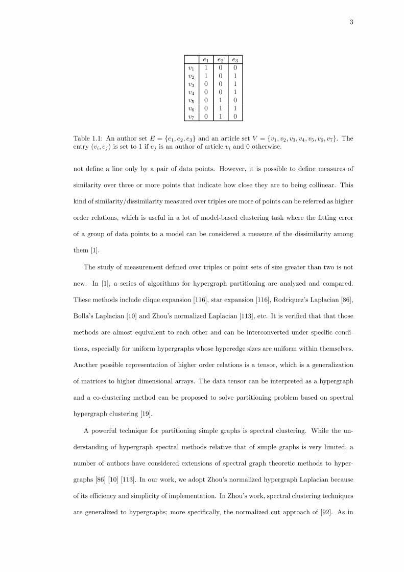
1.1. An author set E = e1, e2, e3 and an article set V = v1, v2, v3, v4, v5, v6, v7.
The entry (vi, ej) is set to 1 if ej is an author of article vi and 0 otherwise. . . . 3
2.1. The similarity matrix for the six data points corresponding to six images in Fig 2.5. 25
2.2. The H matrix for the six data points corresponding to six images in Fig 2.5. Here
each point and its two nearest neighbors are taken as one hyperedge. . . . . . . . 26
3.1. Average accuracy/error for all the experimental frames of every sequence, where
MP means simple graph method by the motion profile, OP means simple graph
method by the optical flow and MP+OP means the simple graph method using
both cues. Mention that for WalkByShop1front.mpg we only consider the case
when K=4. . . . . . . . . . . . . . . . . . . . . . . . . . . . . . . . . . . . . . . . 40
4.1. Average localization errors and standard deviations, computed using Eq. 4.10.
A:Airplanes, C: Cars, F: Faces, M: Motorbikes, W: Watches, K: Ketches) . . . . 62
4.2. The first three tables are confusion matrix for increasing number of Caltech-101
objects from four to six. The average accuracies (%) and the standard deviations
(%) are shown in the tables. Comparison to [62] is reported in the last table.
The numbers in this table are computed from the diagonals of first three tables. . 63
4.3. Results of unsupervised image categorization on both Caltech-101 and Caltech-256. 64
4.4. The first table: average localization errors and standard deviations of the VOC2008,
computed using Eq. 4.10. (P:person, A: Aeroplane, T: Train, B:Boat, M: moto-
bike, H: Horse). The second table: results of unsupervised image categorization
on PASCAL VOC2008. 4-class case: P,A,T,B. 5-class case: P,A,T,B,M. . . . 64
5.1. Selection of the hyperedge size and the vertex degree in the simple graph. We list
the optimal precisions and corresponding K values at different retrieved image
scopes. K denotes the hyperedge size and the vertex degree in the simple graph. 76
ix

List of Figures
1.1. The hypergraph and corresponding simple graph, constructed from the incidence
matrix in Table 1.1. Left: an undirected graph in which two articles are joined
together by an edge if there is at least one author in common. Right: a corre-
sponding hypergraph. . . . . . . . . . . . . . . . . . . . . . . . . . . . . . . . . . 4
2.1. We embedded zoo data set animals into Euclidean space by using the eigenvectors
associated with the second and the third smallest eigenvalues. . . . . . . . . . . . 21
2.2. We embedded zoo data set animals into Euclidean space by using the eigenvectors
associated with the third and the fourth smallest eigenvalues. . . . . . . . . . . . 22
2.3. We embedded zoo data set animals into Euclidean space by using the eigenvectors
associated with the fourth and the fifth smallest eigenvalues. . . . . . . . . . . . 23
2.4. (a): A simple graph of six points in 2-D space. Pairwise distances between vi
and its neighbors are marked on the corresponding edges. (b) The H matrix.
The entry (vi, ej) is set to 1 if a hyperedge ej contains vi, or 0 otherwise. (c):
The corresponding hypergraph w.r.t. the H matrix. The hyperedge weight is
defined as the sum of reciprocals of all the pairwise distances in a hyperedge. (d)
A hypergraph partition which is made on e4. . . . . . . . . . . . . . . . . . . . . 24
2.5. Six images from Caltech-101 [69]. The first three images in the first row are from
the ’ferry’ class; the last three images in the second row are from the ’joshua tree’
class. . . . . . . . . . . . . . . . . . . . . . . . . . . . . . . . . . . . . . . . . . . . 25
x

2.6. The simple graph and corresponding hypergraph, constructed from the similarity
matrix in Table 2.1. Note that in the hypergraph, e3 is cut and the hypergraph
is divided to two groups: v1, v2, v3 and v4, v5, v6. In the simple graph each
data point is corrected to its two nearest neighbors; the edges are cut to form
two groups v1, v2 and v3, v4, v5, v6. The point v3 is not correctly classified in
the simple graph. . . . . . . . . . . . . . . . . . . . . . . . . . . . . . . . . . . . 27
3.1. Illustration of our framework. . . . . . . . . . . . . . . . . . . . . . . . . . . . . 31
3.2. A frame of oversegmentation results extracted from the rocking-horse sequence
used in [97]. . . . . . . . . . . . . . . . . . . . . . . . . . . . . . . . . . . . . . . 33
3.3. Four binary partition results got by the first 4 eigenvectors computed from motion
profile (for one frame of the sequence WalkByShop1cor.mpg, CAVIAR database.
). . . . . . . . . . . . . . . . . . . . . . . . . . . . . . . . . . . . . . . . . . . . . 36
3.4. 4 binary partition results with largest hyperedge weights (for one frame of Walk-
ByShop1cor.mpg ). Obviously that the heperedge got from the 1st and 4th frames
have a good description of objects we want to segment according to their impor-
tance. The computed hyperedge weights are shown below those binary images. . 37
3.5. Segmentation results for the 8th frame of the rocking-horse sequence. (a) The
ground truth, (b) the result by the simple graph based segmentation using optical
flow, (c) the result by the simple graph based segmentation using motion profile,
(d) the result by the simple graph based segmentation using both motion cues,
and (e) the result by the hypergraph cut. . . . . . . . . . . . . . . . . . . . . . . 42
3.6. Segmentation results for the 4th frame of the squirrel sequence. (a) The ground
truth, (b) the result by the simple graph based segmentation using optical flow,
(c) the result by the simple graph based segmentation using motion profile, (d)
the result by the simple graph based segmentation using both motion cues, and
(e) the result by the hypergraph cut. . . . . . . . . . . . . . . . . . . . . . . . . . 43
xi

3.7. Segmentation results for one frame of Walk1.mpg, CAVIAR database. (a) The
ground truth, (b) the result by the simple graph based segmentation using optical
flow, (c) the result by the simple graph based segmentation using motion profile,
(d) the result by the simple graph based segmentation using both motion cues,
and (e) the result by the hypergraph cut. . . . . . . . . . . . . . . . . . . . . . . 44
3.8. Segmentation results for the 16th frame of the car running sequence with occlu-
sion. (a) The ground truth, (b) the result by the simple graph based segmentation
using optical flow, (c) the result by the simple graph based segmentation using
motion profile, (d) the result by the simple graph based segmentation using both
motion cues, and (e) the result by the hypergraph cut. . . . . . . . . . . . . . . 45
3.9. Segmentation results for one frame of the WalkByShop1front.mpg, different colors
denote different clusters in each sub-figure. (a) The ground truth, (b) the result
by the simple graph based segmentation using optical flow (K=2), (c) the result
by the simple graph based segmentation using motion profile (K=2), (d) the
result by the simple graph based segmentation using both motion cues (K=3),
(e) the result by the hypergraph cut (K=2), (f) the result by the hypergraph cut
(K=3), (g) the result by the hypergraph cut (K=4), and (h) the result by the
hypergraph cut (K=5). . . . . . . . . . . . . . . . . . . . . . . . . . . . . . . . . 46
4.1. Illustration of our framework. . . . . . . . . . . . . . . . . . . . . . . . . . . . . . 49
4.2. A hypergraph example and its H matrix. . . . . . . . . . . . . . . . . . . . . . . . . 50
4.3. Positive/Negative set (for a dolphin image) and accumulated intersection scores. Based
on these scores we can decide the features in which bin are ’positive’ or ’negative’. . . . 55
4.4. An illustration on how to get the rough ROI of an unlabeled image. On the second
image 10× 10 dense features are extracted. On the third image the 15 most significant
positive/negative features are shown as red/green ellipses. On the last image the rough
ROI is obtained. . . . . . . . . . . . . . . . . . . . . . . . . . . . . . . . . . . . . . 55
4.5. From left to right: levels l = 0 to l = 2 of the spatial pyramid grids for the
appearance and shape descriptors. . . . . . . . . . . . . . . . . . . . . . . . . . . 57
xii

4.6. The sensitivity analysis on the hyperedge size. the clustering accuracy and its
standard deviation are plotted. Notice that for most of K values, the hypergraph
based method illustrates a much more stable trend of variation on the accuracy. 59
4.7. An illustration for several definitions used in Eq. 4.10. . . . . . . . . . . . . . . . 60
4.8. ROI detection results. The red bounding boxes are the ROI detection results
and the blue boxes are the ground truths. In the first three images very good
detection results are obtained. We also give three examples in which ROIs are
not well detected. . . . . . . . . . . . . . . . . . . . . . . . . . . . . . . . . . . . . 64
4.9. ROI detection results. The first two rows are images from Caltech 256; the last
two rows are images from PASCAL VOC2008. . . . . . . . . . . . . . . . . . . . 65
5.1. Left: A simple graph of six points in 2-D space. Pairwise distances (Dis(i, j))
between vi and its 2 nearest neighbors are marked on the corresponding edges.
Middle: A hypergraph is built, in which each vertex and its 2 nearest neighbors
form a hyperedge. Right: The H matrix of the probability hypergraph shown
above. The entry (vi, ej) is set to the affinity A(j, i) if a hyperedge ej contains
vi, or 0 otherwise. Here A(i, j) = exp(−Dis(i,j)D
), where D is the average distance. 66
5.2. The spatial pyramids for the distance measure based on the appearance descrip-
tors. Three levels of spatial pyramids for the appearance features are: 1×1(whole
image, l = 0), 1 × 3(horizontal bars, l = 1),2 × 2(image quarters, l = 2). . . . . . 73
5.3. Combination of multiple complementary features for image retrieval. Best viewed
in color. . . . . . . . . . . . . . . . . . . . . . . . . . . . . . . . . . . . . . . . . . 77
5.4. Left: the average cost of computation time (ms) to solve the linear system in-
creases rapidly along with the size of H matrix. Right: the precision values (at r
= 20) of different sampling configurations are shown and compared to the proba-
bilistic hypergraph ranking algorithm without random sampling. Here (50, 1000)
means that we randomly sample subsets of 50 unlabelled images for 1000 times. . 78
5.5. Precision vs. scope curves for Corel5K (when full ∆ matrices images are used),
under the passive learning setting. Best viewed in color. . . . . . . . . . . . . . . 79
xiii

5.6. Precision vs. scope curves for Corel5K (when the (50, 1000) random sampling
configuration is used), under the passive learning setting. Best viewed in color. . 80
5.7. Precision vs. scope curves for Corel5K (when full ∆ matrices images are used),
under the active learning setting. Best viewed in color. . . . . . . . . . . . . . . . 81
5.8. Precision vs. scope curves for Corel5K (when the (50, 1000) random sampling
configuration is used), under the active learning setting. Best viewed in color. . . 82
5.9. Per-class precisions for Scene dataset at r = 100 after the 1st round (when full
∆ matrices images are used). Best viewed in color. . . . . . . . . . . . . . . . . . 84
5.10. Per-class precisions for Scene dataset at r = 100 after the 1st round (when the
(50, 1000) random sampling configuration is used). Best viewed in color. . . . . . 85
5.11. The precision-recall curves for Scene dataset under the passive learning setting
(when full ∆ matrices images are used). Best viewed in color. . . . . . . . . . . . 86
5.12. The precision-recall curves for Scene dataset under the passive learning setting
(when the (50, 1000) random sampling configuration is used). Best viewed in color. 87
5.13. The precision-recall curves for Caltech-101 (when full ∆ matrices images are
used). Best viewed in color. . . . . . . . . . . . . . . . . . . . . . . . . . . . . . . 88
5.14. The precision-recall curves for Caltech-101 (when the (50, 1000) random sam-
pling configuration is used). Best viewed in color. . . . . . . . . . . . . . . . . . . 89
xiv

1
Chapter 1
Introduction
1.1 Motivation: Why Hypergraphs
In computer vision and other applied machine learning problems, a fundamental task is to cluster
a set of data in a manner such that elements of the same cluster are more similar to each other
than elements in different clusters. In these problems, we generally assume pairwise relationships
among the objects of our interest. For example, a common distance measure for data points
lying in a vector space is the Euclidean distance, which is used in a lot of unsupervised central
clustering methods such as k -means [79], k -centers clustering [79] and affinity propagation [39].
Actually, a data set endowed with pairwise relationships can be naturally organized as a pairwise
graph (for simplicity, we denote the pairwise graph as simple graph in the following), in which
the vertices represent the objects, and any two vertices that have some kind of relationship are
connected together by a graph edge. The simple graph partitioning problem in mathematics
consists of dividing a graph G into k pieces, such that the pieces are of about the same size and
there are few connections between the pieces. When k = 2, the problem is also referred to as the
graph bisection problem or graph bi-partitioning problem. With a few notable exceptions, the
similarities between objects in a simple graph are utilized to present the pairwise relationships.
The simple graph can be undirected or directed, depending on whether the relationships among
objects are symmetric or not. As to undirected graphs, a typical instance is the graph based
image segmentation, in which pixel to pixel relations can be modelled as undirected edges
because those relations are symmetric. As to directed graphs, a good instance is the World
Wide Web, in which a hyperlink can be taken as a directed edge because the hyperlink based
relationships are asymmetric. Usually a computed kernel matrix is associated to a directed or
undirected graph, a lot of methods for unsupervised and semi-supervised learning can then be

2
formulated in terms of operations on this simple graph and achieve better clustering results
compared to central clustering methods [92] [81] [107].
However, in many real world problems, it is not complete to represent the relations among
a set of objects as simple graphs. This point of view is illustrated in a good example used
in [113]. In this example, a collection of articles need to be grouped into different clusters by
topics. The only information that we have is the authors of all the articles. One way to solve
this problem is to construct an undirected graph in which two vertices are connected by an
edge if they have at least one common author (Table 1.1 and Figure 1.1), and then spectral
graph clustering can be applied [36] [18] [92]. Each edge weight of this undirected graph may be
assigned as the number of authors in common between two articles. It is an easy, nevertheless,
not natural way to represent the relations between the articles because this graph construction
lose the information whether the same person is the author of three or more articles or not. Such
information loss is unexpected because the articles by the same person likely belong to the same
topic and hence the information is useful for our grouping task. A more natural way to remedy
the information is to represent the data points as a hypergraph. An edge in a a hypergraph
is called a hyperedge, which can connect more than two vertices; that is, a hyperedge is a
subset of vertices. For this article clustering problem, it is quite straightforward to construct a
hypergraph with the vertices representing the articles, and the hyperedges the authors (Figure
1). Each hyperedge contains all articles by its corresponding author. Furthermore, positive
weights maybe be put on hyperedges to emphasize or weaken specific authors’ work. For those
authors working on a smaller range of fields, we may assign a larger weight to the corresponding
hyperedge. Compared to simple pairwise graph, in this example hypergraph structure more
completely illustrates the complex relationships among authors and articles.
Another reason to adopt hypergraphs is that, sometimes there does not exist a simple
similarity measure for pairwise data points. Sometimes one may consider the relationship among
three or more data points to determine if they belong to the same cluster. For example, in a
k-lines clustering problem, we need to cluster data points in a d-dimensional vector space into
k clusters where elements in each cluster are well approximated by a line [2]. In this problem,
there does not exist a useful measure of similarity only using pairs of points, because we can
3
e1 e2 e3
v1 1 0 0v2 1 0 1v3 0 0 1v4 0 0 1v5 0 1 0v6 0 1 1v7 0 1 0
Table 1.1: An author set E = e1, e2, e3 and an article set V = v1, v2, v3, v4, v5, v6, v7. Theentry (vi, ej) is set to 1 if ej is an author of article vi and 0 otherwise.
not define a line only by a pair of data points. However, it is possible to define measures of
similarity over three or more points that indicate how close they are to being collinear. This
kind of similarity/dissimilarity measured over triples ore more of points can be referred as higher
order relations, which is useful in a lot of model-based clustering task where the fitting error
of a group of data points to a model can be considered a measure of the dissimilarity among
them [1].
The study of measurement defined over triples or point sets of size greater than two is not
new. In [1], a series of algorithms for hypergraph partitioning are analyzed and compared.
These methods include clique expansion [116], star expansion [116], Rodriquez’s Laplacian [86],
Bolla’s Laplacian [10] and Zhou’s normalized Laplacian [113], etc. It is verified that that those
methods are almost equivalent to each other and can be interconverted under specific condi-
tions, especially for uniform hypergraphs whose hyperedge sizes are uniform within themselves.
Another possible representation of higher order relations is a tensor, which is a generalization
of matrices to higher dimensional arrays. The data tensor can be interpreted as a hypergraph
and a co-clustering method can be proposed to solve partitioning problem based on spectral
hypergraph clustering [19].
A powerful technique for partitioning simple graphs is spectral clustering. While the un-
derstanding of hypergraph spectral methods relative that of simple graphs is very limited, a
number of authors have considered extensions of spectral graph theoretic methods to hyper-
graphs [86] [10] [113]. In our work, we adopt Zhou’s normalized hypergraph Laplacian because
of its efficiency and simplicity of implementation. In Zhou’s work, spectral clustering techniques
are generalized to hypergraphs; more specifically, the normalized cut approach of [92]. As in

4
Figure 1.1: The hypergraph and corresponding simple graph, constructed from the incidencematrix in Table 1.1. Left: an undirected graph in which two articles are joined together by anedge if there is at least one author in common. Right: a corresponding hypergraph.
the case of simple graphs, a real-valued relaxation of the hypergraph normalized cut criterion
leads to the eigen-decomposition of a positive semidefinite matrix called hypergraph laplacian,
which can be regarded as an analogue of the Laplacian for simple graphs [24]. Based on the
concept of hypergraph Laplacian, algorithms can be developed for unsupervised data partition,
hypergraph embedding and transductive inference.
1.2 Contributions
This thesis describes original techniques for the construction of hypergraph models of three
representative computer vision scenarios: video object segmentation, unsupervised image cat-
egorization and relevance feedback image retrieval. In the past decades, simple graph based
methods have been applied in these applications and achieved considerable results. However, as
illustrated above, the expressive power of the hypergraph models places a special emphasis on
5
the relationship among three or more objects, which may make them better models of choice
in computer vision problems. This is in sharp contrast with the more conventional graph rep-
resentation of visual patterns where only pairwise connectivity between objects is described. In
this thesis, we choose to explore hypergraph incidence structures for above three applications.
Through our theoretical discussion and experimental verification, we show that hypergraphs are
better models to represent complex visual patterns on one hand and to keep important struc-
tural information on the other hand. In summary, the contribution of this thesis is fourfold:
(i) For the first time the advantage of the hypergraph neighborhood structure is analyzed.
In our work, two hypergraph based algorithms, hypergraph cut and hypergraph ranking are
adopted to solve optimization problems for computer vision under unsupervised and semi-
supervised learning settings, respectively. We argue that the summarized local grouping infor-
mation contained in hypergraphs causes an ‘averaging’ effect which is beneficial to the clustering
problems in computer vision, just as local image smoothing may be beneficial to the image seg-
mentation task.
(ii) We discuss how to build hypergraph incidence structures and how to solve the related
unsupervised and semi-supervised problems for three different computer vision applications.
We compare our algorithms with state-of-the-art methods and the effectiveness of the proposed
methods is demonstrated by extensive experimentation on various datasets.
(iii) In the application domain of image retrieval, we propose a novel hypergraph model –
probabilistic hypergraph to exploit the structure of the data manifold by considering not only
the local grouping information, but also the similarities between vertices in hyperedges.
(iv) In all three applications mentioned above, we conduct an in depth comparison between
simple graph and hypergraph based algorithms, which is also beneficial to other computer vision
and machine learning applications.
1.3 Overview
The rest of this dissertation is organized as follows. In Chapter 2, we survey the related theoretic
work on unsupervised and semi-supervised hypergraph learning. We lay heavy stress on the
normalized hypergraph Laplacian and spectral hypergraph partitioning algorithms based on
6
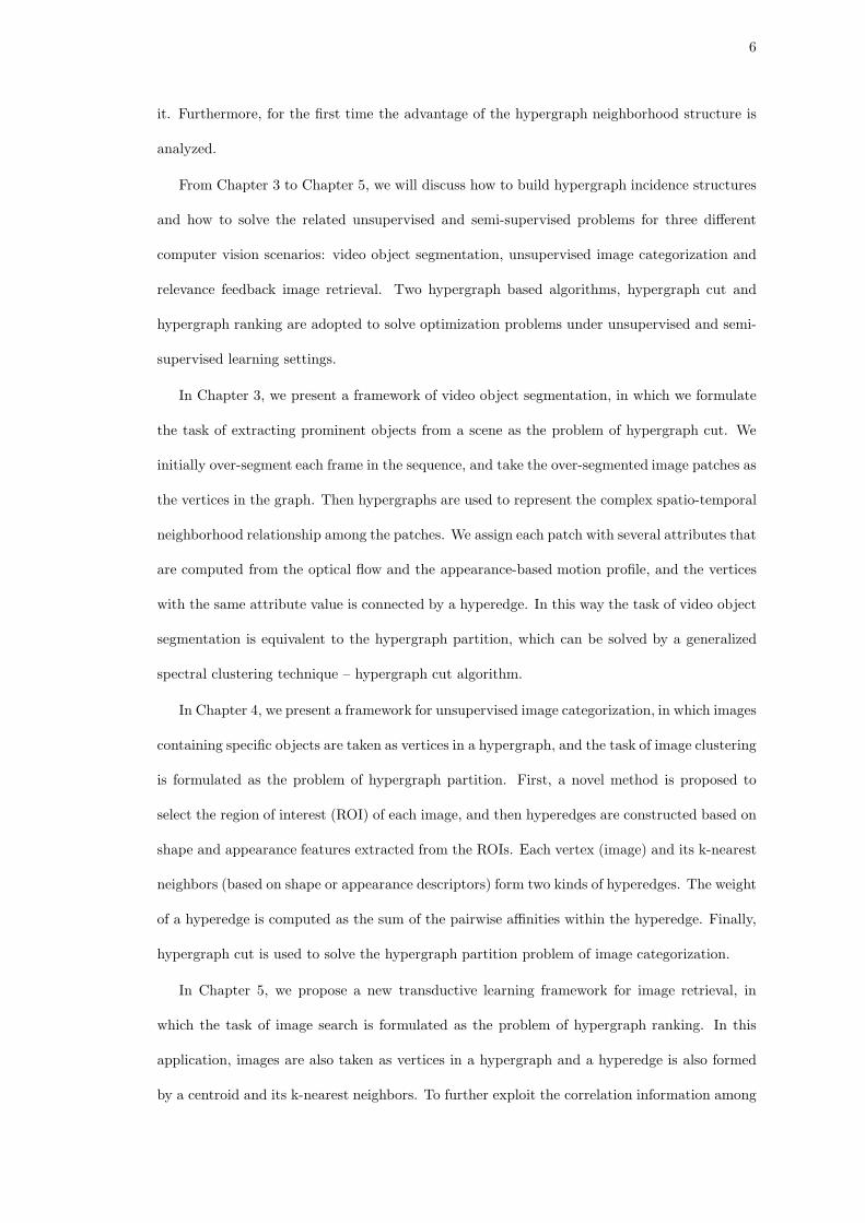
it. Furthermore, for the first time the advantage of the hypergraph neighborhood structure is
analyzed.
From Chapter 3 to Chapter 5, we will discuss how to build hypergraph incidence structures
and how to solve the related unsupervised and semi-supervised problems for three different
computer vision scenarios: video object segmentation, unsupervised image categorization and
relevance feedback image retrieval. Two hypergraph based algorithms, hypergraph cut and
hypergraph ranking are adopted to solve optimization problems under unsupervised and semi-
supervised learning settings.
In Chapter 3, we present a framework of video object segmentation, in which we formulate
the task of extracting prominent objects from a scene as the problem of hypergraph cut. We
initially over-segment each frame in the sequence, and take the over-segmented image patches as
the vertices in the graph. Then hypergraphs are used to represent the complex spatio-temporal
neighborhood relationship among the patches. We assign each patch with several attributes that
are computed from the optical flow and the appearance-based motion profile, and the vertices
with the same attribute value is connected by a hyperedge. In this way the task of video object
segmentation is equivalent to the hypergraph partition, which can be solved by a generalized
spectral clustering technique – hypergraph cut algorithm.
In Chapter 4, we present a framework for unsupervised image categorization, in which images
containing specific objects are taken as vertices in a hypergraph, and the task of image clustering
is formulated as the problem of hypergraph partition. First, a novel method is proposed to
select the region of interest (ROI) of each image, and then hyperedges are constructed based on
shape and appearance features extracted from the ROIs. Each vertex (image) and its k-nearest
neighbors (based on shape or appearance descriptors) form two kinds of hyperedges. The weight
of a hyperedge is computed as the sum of the pairwise affinities within the hyperedge. Finally,
hypergraph cut is used to solve the hypergraph partition problem of image categorization.
In Chapter 5, we propose a new transductive learning framework for image retrieval, in
which the task of image search is formulated as the problem of hypergraph ranking. In this
application, images are also taken as vertices in a hypergraph and a hyperedge is also formed
by a centroid and its k-nearest neighbors. To further exploit the correlation information among

7
images, we propose a fuzzy hypergraph, which assigns each vertex to a hyperedge in a soft way.
In the incidence structure of a fuzzy hypergraph, we describe both the higher order grouping
information and the affinity relationship between vertices within each hyperedge. After feed-
back images are provided, our retrieval system ranks image labels by a transductive inference
approach, which tends to assign the same label to vertices that share many incidental hyper-
edges, with the constraints that predicted labels of feedback images should be similar to their
initial labels.
Finally, Chapter 6 summarizes the contributions of this work, along with a discussion of
future work possibilities.
8
Chapter 2
Unsupervised and Semi-Supervised Learning with
Hypergraphs
In this chapter at first we survey the related theoretic work on hypergraph learning. We survey
a number of approaches from machine learning, VLSI CAD and graph theory that have been
proposed for analyzing the structure of hypergraphs. We mention that there are two basic graph
constructions that underlie all these studies; these constructions are essentially equivalent to
the normalized Laplacian [1]. Then we focus on the derivation of spectral graph hypergraph
theoretic methods for supervised and unsupervised learning, which is the theoretic basis of our
work. At last we give a toy example on how to construct a hypergraph for practical problem.
2.1 Previous Work
The study of measurement defined over triples or point sets of size greater than two is not
new. The primary focus of this literature is the study of topological and geometrical properties
of these generalized measures [77]. While the work on n-metrics is theoretical, more practical
works such as [48] try to measure triadic or higher order distance between its vertices. Multi-
dimensional Scaling(DMS) [11] is a technique for embedding pairwise similarity or dissimilarity
data in a low dimensional Euclidean space, which is used for the purposes of visualization and
a preprocessing step for data analysis methods that require a coordinate representation of their
input. Therefore, some researchers have developed generalizations of MDS to the case of tri-
adic data or higher order data. representitive methods include Carroll & Chang’s work which
developed an algorithm for n-adic MDS using a generalization of the SVD to the case of n-
dimensional matrices [17]; the work of Cox et al. which proposed an MDS algorithm based on
a combination of a Gradient Descent and Isotonic Regression [27]; the works of Joly & LeCalv
and Heiser & Bennani which developed axiomatic theories of triadic distances [52] [58].

9
The initial practical application of hypergraph partitioning algorithms occurs in the field of
VLSI design and synthesis [2], which involves the partitioning of large circuits into k equally
sized parts in a manner that minimizes the connectivity between the parts. In this applica-
tion, the circuit elements are the vertices of the hypergraph and the nets that connect these
circuit elements are the hyperedges [3]. The development of the tools for partitioning these
hypergraphs is almost entirely heuristic and very little theoretical work exists that analyzes
their performance beyond empirical benchmarks. The leading tools are based on two phase
multi-level approaches [60]. In the first phase, a hierarchy of hypergraphs is constructed by in-
crementally collapsing the hyperedges of the original hypergraph according to some measure of
homogeneity. In the second phase, starting from a partitioning of the hypergraph at the coarsest
level, the algorithm works its way down the hierarchy and at each stage the partitioning at the
level above serves as an initialization for the next level [35] [61].
The set of tools available for partitioning graphs are generalized and used on hypergraphs.
An example is the generalization of Graph-Cut algorithms [14] for solving the max-flow min-cut
problem on hypergraphs [83]. Some works consider to construct a graph that approximates the
hypergraph and partition it; this partition in turn induces a vertex partitioning on the original
hypergraph. Other works try to construct methods that operate directly on the hypergraph
while implicitly working on its graph approximation. In this sense the previously proposed
algorithms for partitioning a hypergraph can be divided into two categories. The first category
aims at constructing a simple graph from the original hypergraph, and then partitioning the
vertices by spectral clustering techniques. These methods include clique expansion [116], star
expansion [55], Rodriquez’s Laplacian [86] and clique averaging [2] etc. Clique Expansion and
Star Expansion are two most commonly used graph approximations. Clique Expansion, as the
name suggests, expands each hyperedge into a clique. Star expansion introduces a dummy
vertex for each hyperedge and connects each vertex in the hyperedge to it [55]. As can be
expected, the weights on the edges of the clique and the star determine the cut properties of the
approximating graph [47] [57]. Another method to approximate the hypergraph using a weighted
graph is clique averaging, which is closely related to clique expansion but is able to preserve
more information contained in original hypergraphs. The second category of approaches define
10
a hypergraph ‘Laplacian’ using analogies from the simple graph Laplacian. Representative
methods in this category include Bolla’s Laplacian [10], Zhou’s normalized Laplacian [113], etc.
In [1], the above algorithms are analyzed and verified that they are equivalent to each other
under specific conditions.
Another possible representation of higher order relations is a tensor, which is a generalization
of matrices to higher dimensional arrays. In recent years, co-clustering of data with two or more
than two types of entities has attracted increasing attention. The task of co-clustering is to
simultaneously cluster the different types of entities. Bi-clustering is the name for co-clustering
when there are two types of data need to be clustered. In this case not only the objects but also
the features of the objects are clustered; i.e., the data is represented in a data matrix and the
row and columns are clustered simultaneously. For example, in the text-mining scenario, we
need to co-cluster documents and keywords, where a keyword is related to a document by the
number of its occurrences in the document. The co-clustering of bi-type heterogeneous data has
been widely investigated in a number of works such as [5] [31] [21]. If the data have more than
two types, they can be represented as higher dimensional arrays. A real life example is audience-
movies-casts in the film rating (collaborative filtering) scenario, where an audience gives a rating
to a film that is cast by several actors or actresses. Although it is possible to cluster each type
separately, but this approach would miss the potential leveraging that could be obtained from
the interrelationships among different types. Representative work includes [7] [73] [74] which
generalize bi-type methods for multi-type data, and [4] [20] which consider the interrelationships
among all the entity types. In [19], the data tensor is interpreted as a hypergraph and propose
a coclustering method based on spectral hypergraph partitioning.
2.2 Notation and Terminology
The key difference between the hypergraph and the simple graph lies in that the former uses
a subset of the vertices as an edge, i.e., a hyperedge connecting more than two vertices. Let
V represent a finite set of vertices and E a family of subsets of V such that⋃
e∈E = V ,
G = (V, E, w) is called a hypergraph with the vertex set V and the hyperedge set E, and each
hyperedge e is assigned a positive weight w(e). For a vertex v ∈ V , its degree is defined to be
11
d(v) =∑
e∈E|v∈e w(e). For a hyperedge e ∈ E, its degree is defined by δ(e) = |e|. Let us
use Dv,De, and W to denote the diagonal matrices of the vetex degrees, the hyperedge degrees,
and the hyperedge weights respectively. The hypergraph G can be represented by a |V | × |E|
matrix H which h(v, e) = 1 if vH ∈ eH and 0 otherwise. According to the definition of H ,
d(v) =∑
e∈E w(e)h(v, e) and δ(e) =∑
v∈V h(v, e).
For a vertex subset S ⊂ V , let Sc denote the compliment of S. A cut of a hypergraph
G = (V, E, w) is a partition of V into two parts S and Sc. We say that a hyperedge e is cut if
it is incident with the vertices in S and Sc simultaneously.
Given a vertex subset S ⊂ V , define the hyperedge boundary ∂S of S to be a hyperedge set
which consists of hyperedges which are cut:
∂S := e ∈ E|e ∩ S 6= ∅, e ∩ Sc 6= ∅. (2.1)
Define the volume volS of S to be the sum of the degrees of the vertices in S, that is, volS :=
∑
v ∈ Sd(v). Moreover, define the volume of ∂S by
vol∂S :=∑
e∈∂S
w(e)|e ∩ S||e ∩ Sc|
|δ(e)| . (2.2)
According to Equation 2.2, we have vol∂S = vol∂Sc. The definition given by above equations
can be understood as follows: if we treat the defined volume of the hyperedge boundary across
S and Ss as the connection between two clusters and the volume of S or Sc as the connection
inside S or Sc, we try to obtain a partition in which the connection among the vertices in
the same cluster is dense while the connection between two clusters is sparse. Then a natural
partition can be formalized as follows:
arg min∅6=S⊂V
c(S) := vol(S, Sc)
(
1
vol(S)+
1
vol(Sc)
)
(2.3)
For a simple graph, |e⋂S| = |e⋂Sc| = 1, and δ(e) = 2. According to the derivation in [19],
the right-hand side of above equation reduces to the simple graph normalized cut [92] up to a
factor 12 .

12
2.3 Hypergraph Learning Algorithms
In this section we introduce a number of existing methods for hypergraph learning which are
surveyed in [1] and [2]. At first we present the methods which construct a graph representation
using the initial structure of hypergraph. Then we introduce other methods define various hyper-
graph Laplacians. Particularly we focus on the derivation of normalized hypergraph Laplacian
for supervised and unsupervised learning, which is the theoretic basis of our work.
2.3.1 Star Expansion
The star expansion algorithm constructs a graph G∗(V ∗, E∗) from original hypergraph G(V, E)
by introducing a new vertex for every hyperedge e ∈ E, thus V ∗ = V⋃
E [116]. It connects the
new graph vertex e to each vertex in the hyperedge to it, i.e. E∗ = (u, e) : u ∈ e, e ∈ E. Each
hyperedge in E has a corresponding star in the graph G∗ and that G∗ is a bi-partite graph.
Star expansion assigns the scaled hyperedge weight to each corresponding graph edge:
w∗(u, e) =w(e)
δ(e)(2.4)
Then the combinatorial or normalized Laplacian of the constructed simple graph is used to
cluster vertices.
2.3.2 Clique Expansion
The clique expansion algorithm [116] constructs a graph Gx(V, ExV 2) from the original hyper-
graph G(V, E) by replacing each hyperedge e = (u1, ..., uδ(e)) ∈ E with an edge for each pair
of vertices in the hyperedge: Ex = (u, v) : u, v ∈ e, e ∈ E. The vertices in hyperedge e form a
clique in the graph Gx. The edge weight wx(u, v) minimizes the difference between the weight
of the graph edge and the weight of each hyperedge e that contains both u and v:
wx(u, v) = arg minwx(u,v)
∑
e∈E:u,v∈e
(wx(u, v) − w(e))2. (2.5)
The solution of this criterion is

13
wx(u, v) =1
µ(n, k)
∑
e∈E:u,v∈e
w(e). (2.6)
where µ(n, k) =
n − 2
k − 2
is the number of hyperedges that contain a particular pair of vertices;
k is the size of the hyperedge and |V | = n. The relationship between a hyperedge and the edge
weights in its clique in the above approach was the simplest possible, where one assumes that
the hyperedge weight and the edge weights are equal to each other.
2.3.3 Clique Averaging
In [1], a new algorithm is proposed to transfer a hypergraph into a simple graph. In the method
of clique averaging, the relationship between a hyperedge weight and its related simple graph
weights are defined as follows:
w(e) =
k
2
−1
∑
ei,ej inE,i<j
w(vi, vj). (2.7)
the above equation states that the L1 norm of the clique weights is proportional to the hyperedge
weight. Without loss of generality we will assume that the set of hyperedges has been ordered
in a lexicographic order based on the vertices incident on each hyperedge. A similar ordering is
done on the set of graph edges too. We can now define the incidence matrix Υ. Υ is a zero-one
matrix, that represents the incidence relationship between a hyperedge in a hypergraph and an
edge in the related simple graph.
Υi,j =
1, if edge j is incident on hyperedge i
0, otherwise.
(2.8)
Denote d2 as the vector of graph edge weights of length(
n2
)
and, denote dk the vector of
hyperedge weights. Then Equation 2.7 can be written in matrix form as
(
k
2
)
Υd2 = dk. (2.9)

14
This equation assumes that d2 ≥ 0, i.e., each element of the vector d2 is non-negative. If we
enforce an upper bound d2 ≤ 1 also, the graph approximation of hypergraph is given by the
edge weight vector d2 that minimizes the following constrained minimization problem:
mind2
‖(
k
2
)
Υd2 − dk‖2F , 0 ≤ d2 ≤ 1. (2.10)
Actually, this method is closely related to clique expansion. Denote de2 as the vector of approx-
imation graph edge weights, we can derive the following equation from the solution equation of
Clique Expansion 2.24:
µ(n, k)Υde2 = ΥΥ>dk. (2.11)
Neglect the constants in Equations 2.9 and 2.11, they differ only in the right hand side by a
pre-multiplication by the matrix ΥΥ>. This is a symmetric matrix, the effect of multiplying this
matrix to dk is equivalent to a convolution of the hyperedge weights by a quadratically decreasing
kernel [1]. Thus ΥΥ>dk is a low passed version of dk. This implies that Clique Expansion solves
the same approximation problem as Clique Averaging, but instead of operating on the original
hypergraph it operates on a low passed version of it. Although the approximation produced by
Clique Averaging is of a higher quality theoretically, in practice there is virtually no difference
between their performance, especially when values of σ are chosen carefully [2] (the parameter
σ is used to convert a dissimilarity d into the affinity exp(−d/σ)).
2.3.4 Bolla’s Laplacian
Bolla defines a Laplacian for an unweighted hypergraph in terms of the diagonal vertex degree
matrix Dv, the diagonal edge degree matrix De, and the incidence matrix H [10]:
Lo := Dv − HD−1e H>. (2.12)
According to [10], the eigenvectors of Bolla’s Laplacian Lo define the ‘best’ Euclidean embedding
of the hypergraph. Bolla also shows a relationship between the spectral properties of Lo and
the minimum cut of the hypergraph.

15
2.3.5 Rodriguez’s Laplacian
In [86] a weighted graph Gr(V, Er = Ex) is constructed from an unweighted hypergraph
G(V, E). Like clique expansion, each hyperedge is replaced by a clique in the graph Gr. The
weight wr(u, v) of an edge is set to the number of edges containing both u and v:
wr(u, v) = |e ∈ E : u, v ∈ e|. (2.13)
Then the graph Laplacian applied to Gr is expressed in terms of the hypergraph structure:
Lr(Gr) = Drv − HH>, (2.14)
where Drv is the vertex degree matrix of the graph Gr. Like Bolla, Rodriguez also shows a
relationship between the spectral properties of Lr and the cost of minimum partitions of the
hypergraph.
2.3.6 Gibson’s Dynamical System
In [42] the authors have proposed a dynamical system to cluster categorical data that can be
represented using a hypergraph. They consider the following iterative process:
1. sn+1i,j =
∑
e:i∈e
∑
k 6=i∈e wesnk,j
2. Orthonormalize the vectors snj .
And it is proven that the iterative procedure described above is the power method for calculating
the eigenvectors of the adjacency matrix S = Dv − HWH top.
2.3.7 Li’s Adjacency Matrix
[71] formally define properties of a regular, unweighted hypergraph G(V, E) in terms of the star
expansion of the hypergraph. In particular, they define the |V | × |V | adjacency matrix of the
hypergraph, HH>. They show a relationship between the spectral properties of the adjacency
matrix of the hypergraph HH> and the structure of the hypergraph.
16
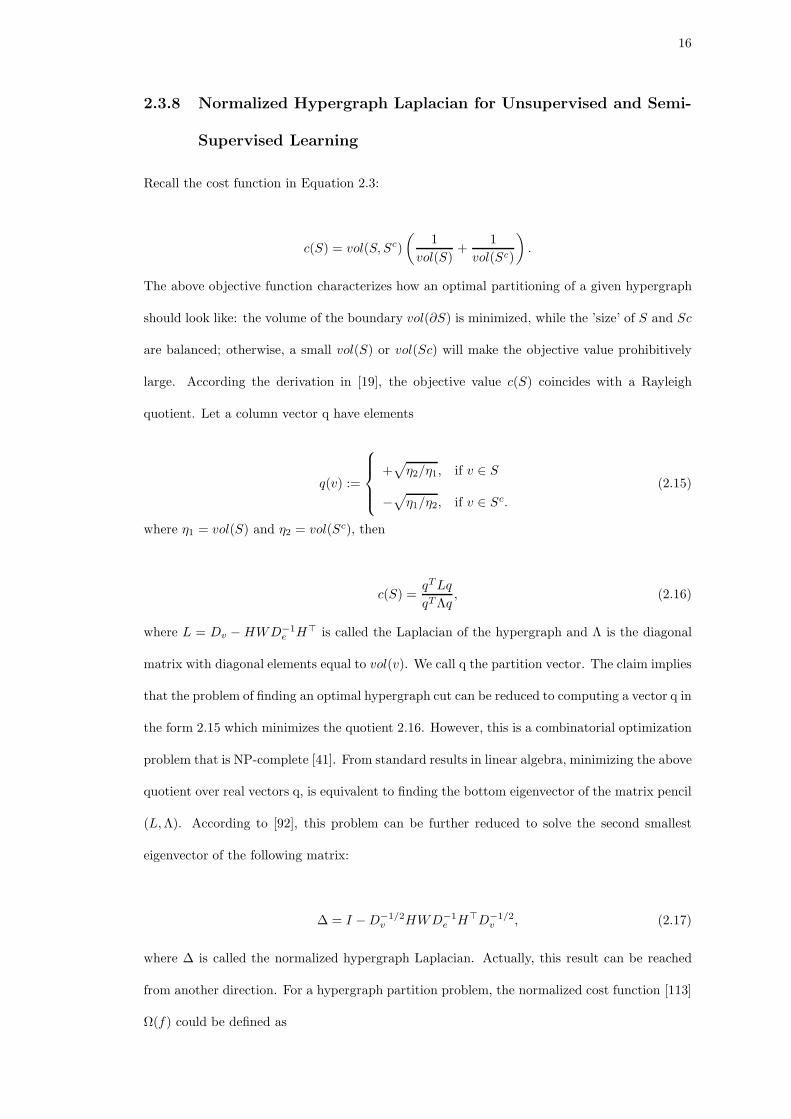
2.3.8 Normalized Hypergraph Laplacian for Unsupervised and Semi-
Supervised Learning
Recall the cost function in Equation 2.3:
c(S) = vol(S, Sc)
(
1
vol(S)+
1
vol(Sc)
)
.
The above objective function characterizes how an optimal partitioning of a given hypergraph
should look like: the volume of the boundary vol(∂S) is minimized, while the ’size’ of S and Sc
are balanced; otherwise, a small vol(S) or vol(Sc) will make the objective value prohibitively
large. According the derivation in [19], the objective value c(S) coincides with a Rayleigh
quotient. Let a column vector q have elements
q(v) :=
+√
η2/η1, if v ∈ S
−√
η1/η2, if v ∈ Sc.
(2.15)
where η1 = vol(S) and η2 = vol(Sc), then
c(S) =qT Lq
qT Λq, (2.16)
where L = Dv − HWD−1e H> is called the Laplacian of the hypergraph and Λ is the diagonal
matrix with diagonal elements equal to vol(v). We call q the partition vector. The claim implies
that the problem of finding an optimal hypergraph cut can be reduced to computing a vector q in
the form 2.15 which minimizes the quotient 2.16. However, this is a combinatorial optimization
problem that is NP-complete [41]. From standard results in linear algebra, minimizing the above
quotient over real vectors q, is equivalent to finding the bottom eigenvector of the matrix pencil
(L, Λ). According to [92], this problem can be further reduced to solve the second smallest
eigenvector of the following matrix:
∆ = I − D−1/2v HWD−1
e H>D−1/2v , (2.17)
where ∆ is called the normalized hypergraph Laplacian. Actually, this result can be reached
from another direction. For a hypergraph partition problem, the normalized cost function [113]
Ω(f) could be defined as

17
1
2
∑
e∈E
∑
u,v∈e
w(e)h(u, e)h(v, e)
δ(e)
(
f(u)√
d(u)− f(v)√
d(v)
)2
, (2.18)
where the vector f is the image labels to be learned. By minimizing this cost function, vertices
sharing many incidental hyperedges are guaranteed to obtain similar labels. Defining Θ =
D− 1
2v HWD−1
e HT D− 1
2v , we can derive Equation 5.4 as follows:
Ω(f) =∑
e∈E
∑
u,v∈e
w(e)h(u, e)h(v, e)
δ(e)
(
f2(u)
d(u)− f(u)f(v)√
d(u)d(v)
)
=∑
u∈V
f2(u)∑
e∈E
w(e)h(u, e)
d(u)
∑
v∈V
h(v, e)
δ(e)
−∑
e∈E
∑
u,v∈e
f(u)h(u, e)w(e)h(v, e)f(v)√
d(u)d(v)δ(e)
= fT (I − Θ)f, (2.19)
where I is the identity matrix. Above derivation shows that (i) Ω(f, w) = fT (I − Θ)f if and
only if∑
v∈V
h(v,e)δ(e) = 1 and
∑
e∈E
w(e)h(u,e)d(u) = 1, which is true because of the definition of δ(e)
and d(u); (ii) ∆ = I − Θ is a positive semi-definite matrix introduced above – the normalized
hypergraph Laplacian and Ω(f) = fT ∆f . The above cost function has the similar formulation
to the normalized cost function of a simple graph Gs = (Vs, Es):
Ωs(f) =1
2
∑
vi,vj∈Vs
As(i, j)
(
f(i)√Dii
− f(j)√
Djj
)2
= fT (I − D− 12 AsD
− 12 )f = fT ∆sf, (2.20)
where D is a diagonal matrix with its (i, i)-element equal to the sum of the ith row of the affinity
matrix As; ∆s = I −Θs = I −D− 12 AsD
− 12 is called the normalized simple graph Laplacian. In
an unsupervised framework, Equation 5.4 and Equation 5.6 can be optimized by the eigenvector
related to the smallest nonzero eigenvalue of ∆ and ∆s [113], respectively.
In the transductive learning setting [113], we define a vector y to introduce the labeling
information and to assign their initial labels to the corresponding elements of y: y(v) = 1, if a
vertex v is in the positive set Pos, y(v) = −1, if it is in the negative set Neg. If v is unlabeled,

18
y(v) = 0. To force the assigned labels to approach the initial labeling y, a regularization term
is defined as follows:
‖f − y‖2 =∑
u∈V
(f(u) − y(u))2. (2.21)
After the feedback information is introduced, the learning task is to minimize the sum of two
cost terms with respect to f [112] [113], which is
Φ(f) = fT ∆f + µ‖f − y‖2, (2.22)
where µ > 0 is the regularization parameter. Differentiating Φ(f) with respect to f , we have
f = (1 − γ)(I − γΘ)−1y, (2.23)
where γ = 11+µ . This is equivalent to solving the linear system ((1 + µ)I − Θ) f = µy.
For the simple graph, we can simply replace Θ with Θs to fulfill the transductive learning.
2.3.9 The Connections between Hypergraph Learning Algorithms
In [1], different hypergraph learning algorithms are analyzed and proved to be equivalent to
each other. At first, [1] verifies that for a k-uniform hypergraph (each hyperedge contains a
fixed number of k vertices),the eigenvectors of the normalized Laplacian for the bipartite graph
G∗c (obtained from Star Expansion) are exactly the eigenvectors of the normalized Laplacian
for the standard clique expansion graph Gx. This is a surprising result since the two graphs
are completely different in the number of vertices and the connectivity between these vertices.
Even for non-uniform hypergraphs, the difference between two formulations are not large and
may obtain similar decomposed eigenvectors.
[1] also proved that all different hypergraph Laplacians correspond to either clique or star
expansion of the original hypergraph under specific conditions. Bolla’s Laplacian corresponds to
the unnormalized Laplacian of the associated clique expansion with the appropriate weighting
function. The Rodriguez Laplacian can similarly be shown to be the unnormalized Laplacian
of the clique expansion of an unweighted graph with every hyperedge weight set to 1. Gibson’s

19
algorithm calculates the eigenvectors of the adjacency matrix for the clique expansion graph.
For Zhou’s normalized Laplacian, it is equivalent to constructing a star expansion and using
the normalized Laplacian defined on it.
2.4 Toy Examples
In this section, we quote two examples to explain how to construct hypergraphs for practical
problems. The first example is also used in Zhou’s work [113].
In the first example, the zoo data set from UCI Machine Learning Depository [38] is used.
The zoo data set is usually referred to as the so-called categorical data. It contains totally 7
types and 101 animals:
1 – (41 kinds of animals) aardvark, antelope, bear, boar, buffalo, calf, cavy, cheetah, deer,
dolphin, elephant, fruitbat, giraffe, girl, goat, gorilla, hamster, hare, leopard, lion, lynx, mink,
mole, mongoose, opossum, oryx, platypus, polecat, pony, porpoise, puma, pussycat, raccoon,
reindeer, seal, sealion, squirrel, vampire, vole, wallaby,wolf;
2 – (20 kinds of animals) chicken, crow, dove, duck, flamingo, gull, hawk, kiwi, lark, ostrich,
parakeet, penguin, pheasant, rhea, skimmer, skua, sparrow, swan, vulture, wren;
3 – (5 kinds of animals) pitviper, seasnake, slowworm, tortoise, tuatara;
4 – (13 kinds of animals) bass, carp, catfish, chub, dogfish, haddock, herring, pike, piranha,
seahorse, sole, stingray, tuna;
5 – (4 kinds of animals) frog, frog, newt, toad;
6 – (8 kinds of animals) flea, gnat, honeybee, housefly, ladybird, moth, termite, wasp;
7 – (10 kinds of animals) clam, crab, crayfish, lobster, octopus, scorpion, seawasp, slug,
starfish, worm.
Specifically, each instance in this dataset is described by one or more attributes. Each at-
tribute takes only a small number of values, each corresponding to a specific category. Attribute
values cannot be naturally ordered linearly as numerical values. Totally there are 16 attributes
as follows:
1. hair: Boolean
2. feathers: Boolean

20
3. eggs: Boolean
4. milk: Boolean
5. airborne: Boolean
6. aquatic: Boolean
7. predator: Boolean
8. toothed: Boolean
9. backbone: Boolean
10. breathes: Boolean
11. venomous: Boolean
12. fins: Boolean
13. legs: Numeric (set of values: 0,2,4,5,6,8)
14. tail: Boolean
15. domestic: Boolean
16. catsize: Boolean
In our experiments, we constructed a hypergraph for the zoo dataset, where attribute values
were regarded as hyperedges. For Boolean attribute, we construct two hyperedges according to
the value of each animal on each attribute (‘true’ or ‘false’). For numeric value attribute (the
attribute 13), we construct 6 hyperedges, according to the numerical value of each animal on
this attribute. Then we totally get 36 hyperedges. The weights for all hyperedges were simply
set to 1. How to choose suitable weights is definitely an important problem requiring additional
exploration however.
The first task we addressed is to embed the animals in the zoo dataset into Euclidean space.
We embedded those animals into Euclidean space by using the eigenvectors of the hypergraph
Laplacian associated with the smallest eigenvalues. In Figure 2.1, the eigenvectors associated
with the second and the third smallest eigenvalues are used as x and y coordinates. All the
animals are illustrated in this figure and animals in a specific type use a specific text color. For
example, all the mammals are shown red in Figure 2.1.
From this figure, It is apparent that most animals are well separated according their type
in their Euclidean representations. For example, all the mammals distribute on the left hand

21
−0.15 −0.1 −0.05 0 0.05 0.1 0.15
−0.2
−0.15
−0.1
−0.05
0
0.05
0.1
0.15
aardvark
antelope
bass
bearboar
buffalocalf
carp
catfish
cavy
cheetah
chicken
chub
clamcrabcrayfish
crow
deer
dogfish
dolphin
dove
duck
elephant
flamingo
flea
frogafrog
b
fruitbat
giraffegirl
gnat
goat gorilla
gull
haddock
hamsterhare
hawk
herring
honeybeehousefly
kiwi ladybird
lark
leopardlion
lobster
lynx
mink
molemongoose
moth
newt
octopus
opossumoryx
ostrich
parakeet
penguin
pheasant
pikepiranha
pitviper
platypuspolecat
pony
porpoise
pumapussycat
raccoon
reindeer
rhea
scorpion
seahorse
seal
sealion
seasnake
seawasp
skimmerskua
slowworm
slug
sole
sparrow
squirrel
starfish
stingray
swan
termite
toad
tortoise
tuatara
tuna
vampire
vole
vulture
wallaby
wasp
wolfworm
wren
Figure 2.1: We embedded zoo data set animals into Euclidean space by using the eigenvectorsassociated with the second and the third smallest eigenvalues.
side of Figure 2.1; all the fishes distribute on the bottom of the graph. Moreover, it deserves
a further look on the transition area of the graph. Platypus is significantly mapped to the
positions between class 1 (mammals), and class 3 (reptiles). A similar observation also holds
for sea-snake, which is very close to fish. Even in Figure 2.2 and Figure 2.3, we can still find
that animals distribute intensively according to their category.
The second example is illustrated in Figure 2.4, which shows an example to explain how
to construct a hypergraph. v1, v2, ..., v6 are six points in a 2-D space and their interrelation-
ships could be represented as a simple graph, in which pairwise distances between every vertex
and its neighbors are marked on the corresponding edges. Assuming that each vertex and
its two-nearest neighbors form a hyperedge, a vertex-hyperedge matrix H could be given as
Figure 2.4(b). For example, the hyperedge e4 is composed of vertex v4 and its two nearest

22
−0.2 −0.15 −0.1 −0.05 0 0.05 0.1 0.15
−0.15
−0.1
−0.05
0
0.05
0.1
0.15
0.2
0.25
aardvark
antelope
bass
bear
boarbuffalocalf
carpcatfish
cavy
cheetah
chicken
chub
clamcrab
crayfish
crow
deer
dogfishdolphin
doveduck
elephant
flamingo
flea
froga
frogb
fruitbat
giraffegirl
gnat
goatgorilla
gull
haddock
hamsterhare
hawk
herring
honeybee
housefly
kiwi
ladybird
lark
leopardlion
lobster
lynxmink
molemongoose
moth
newt
octopus
opossumoryx
ostrich parakeetpenguin
pheasant
pikepiranha
pitviperplatypus
polecat pony
porpoise
pumapussycatraccoonreindeer
rhea
scorpion
seahorse
seal
sealion
seasnake
seawasp
skimmerskua
slowworm
slug
sole
sparrow
squirrel
starfish
stingray
swan
termite
toad
tortoisetuatara
tuna
vampire
vole
vulture
wallaby
wasp
wolf
worm
wren
Figure 2.2: We embedded zoo data set animals into Euclidean space by using the eigenvectorsassociated with the third and the fourth smallest eigenvalues.

23
−0.15 −0.1 −0.05 0 0.05 0.1 0.15 0.2 0.25−0.4
−0.3
−0.2
−0.1
0
0.1
0.2
aardvark
antelope
bass
bearboar
buffalo
calf
carp
catfish
cavy
cheetah
chicken
chub
clam
crab
crayfish
crow
deerdogfish
dolphin
dove
duck elephantflamingo
flea
froga frog
b
fruitbat
giraffegirl
gnatgoat
gorilla
gull
haddock hamster
hare
hawk
herring
honeybee
housefly
kiwi
ladybirdlark
leopardlion
lobster
lynxmink
mole
mongoose
moth
newt
octopus
opossum
oryx
ostrich
parakeet
penguin
pheasantpike
piranha
pitviper
platypuspolecat
pony
porpoise
puma
pussycat
raccoon
reindeer
rhea
scorpion
seahorse
seal
sealion seasnakeseawasp
skimmerskua
slowworm
slug
sole
sparrowsquirrel
starfish
stingray
swan
termitetoad
tortoisetuatara
tuna
vampirevole
vulture
wallaby
wasp
wolf
worm
wren
Figure 2.3: We embedded zoo data set animals into Euclidean space by using the eigenvectorsassociated with the fourth and the fifth smallest eigenvalues.

24
neighbors v3 and v5. Among all the hyperedges constructed in this example, e1, e2, e3 corre-
spond to the vertices subset v1, v2, v3 and e5, e6 correspond to the vertices subset v4, v5, v6
(Figure 2.4(c)). To measure the affinity among the vertices in each hyperedge, we can define
the hyperedge weight as the sum of reciprocals of all the pairwise distances in a hyperedge.
Figure 2.4: (a): A simple graph of six points in 2-D space. Pairwise distances between vi andits neighbors are marked on the corresponding edges. (b) The H matrix. The entry (vi, ej) isset to 1 if a hyperedge ej contains vi, or 0 otherwise. (c): The corresponding hypergraph w.r.t.the H matrix. The hyperedge weight is defined as the sum of reciprocals of all the pairwisedistances in a hyperedge. (d) A hypergraph partition which is made on e4.
In order to bipartition the hypergraph in Figure 2.4(c)), intuitively the hyperedges with
the smallest weights should be removed, and at the same time as many hyperedges with larger
weights as possible should be kept. Since e4 has the smallest hyperedge weight, a hypergraph
partition could be made on it (Figure 2.4(d)) to classify v1, v2, ..., v6 into two groups. This is
exactly the result obtained by normalized hypergraph cut.

25
Figure 2.5: Six images from Caltech-101 [69]. The first three images in the first row are fromthe ’ferry’ class; the last three images in the second row are from the ’joshua tree’ class.
v1 v2 v3 v4 v5 v6
v1 1.0000 0.5342 0.4795 0.2566 0.4558 0.2667v2 0.5342 1.0000 0.4603 0.2935 0.4311 0.2758v3 0.4795 0.4603 1.0000 0.5976 0.6547 0.6083v4 0.2566 0.2935 0.5976 1.0000 0.7062 0.8245v5 0.4558 0.4311 0.6547 0.7062 1.0000 0.7804v6 0.2667 0.2758 0.6083 0.8245 0.7804 1.0000
Table 2.1: The similarity matrix for the six data points corresponding to six images in Fig 2.5.
2.5 Analysis of the Advantage of the Hypergraph Structure
In order to better explain the neighborhood structure of hypergraphs, we can revisit the Clique
Expansion [116] algorithm and inversely transfer a hypergraph into a simple graph. Clique
Expansion builds a new simple graph from a hypergraph by replacing each hyperedge with
edges for each pair of vertices in the hyperedge. In this new simple graph, the pairwise edge
weight between two vertices is proportional to the sum of their incident hyperedge weights:
wx(u, v) =1
µ(n, k)
∑
e inE:u,v∈e
w(e). (2.24)
According to the analysis in Agarwal’s work [1], for a uniform hypergraph, it is verified that the
eigenvectors of the hypergraph normalized Laplacian are equivalent to the eigenvectors of the
simple graph obtained by Clique Expansion. For a nonuniform hypergraph, the eigenvectors

26
e1 e2 e3 e4 e5 e6
v1 1 1 0 0 0 0v2 1 1 0 0 0 0v3 1 1 1 0 0 0v4 0 0 0 1 1 1v5 0 0 1 1 1 1v6 0 0 1 1 1 1
Table 2.2: The H matrix for the six data points corresponding to six images in Fig 2.5. Hereeach point and its two nearest neighbors are taken as one hyperedge.
of the simple graph obtained by Clique Expansion is very close to those of the hypergraph
normalized Laplacian. Consider that we take the sum of the pairwise similarities inside a
hyperedge as the hyperedge weight (similar configurations are used in the following chapters).
We transfer this hypergraph into a simple graph by Clique Expansion. In the obtained simple
graph, the edge weight between two vertices vi and vj is not decided by the pairwise affinity
Ai,j between two vertices, but the averaged neighboring affinities close to them; furthermore,
this edge weight is influenced more by those pairwise affinities whose two incident vertices
share more hyperedges with vi and vj . Through the hyergraph, the ‘higher order’ or ‘local
grouping’ information is used for the construction of graph neighborhood. We argue that such
an ‘averaging’ effect may be beneficial to the image clustering task, just as local image smoothing
may be beneficial to the image segmentation task.
To clearly show the advantage of the hypergraph model over simple graph based model,
here we present an example including six images from two classes, shown in Figure 2.5. In Fig-
ure 2.6, these six images are denoted as six vertices v1, v2, ..., v6 and pairwise affinities between
each pair of vertices are presented in the matrix At( Table 2.1). A simple graph is built in Fig-
ure 2.6(above), in which each vertex is connected to its two nearest neighbors. The edge weight
between two vertices equals their pairwise affinity if there is an edge between them; otherwise it
is set to be 0. Intuitively this simple graph can be partitioned by removing two weakest edges
v1v3 and v2v3. This is the result of the normalized cut to minimize the follow formula:
NScut(S, Sc) := Scut(S, Sc)
(
1
assoc(S, V )+
1
assoc(Sc, V )
)
, (2.25)
where Scut(S, Sc) =∑
u∈S,v∈Sc ws(u, v) and ws(u, v) is a simple graph edge weight between
u and u; assoc(S, V ) =∑
u∈S,v∈V ws(u, v) and assoc(Sc, V ) is similarly defined. According to

27
Figure 2.6: The simple graph and corresponding hypergraph, constructed from the similaritymatrix in Table 2.1. Note that in the hypergraph, e3 is cut and the hypergraph is divided totwo groups: v1, v2, v3 and v4, v5, v6. In the simple graph each data point is corrected to itstwo nearest neighbors; the edges are cut to form two groups v1, v2 and v3, v4, v5, v6. Thepoint v3 is not correctly classified in the simple graph.
this criterion, v3 (a ferry) is falsely classified into the ‘joshua tree’ class.
For comparison, we construct a hypergraph in Figure 2.6(Bottom). Let each vertex and
its two-nearest neighbors form a hyperedge, a vertex-hyperedge matrix H could be formed
(Table 2.1). Among all the hyperedges constructed in this example, e1 and e2 correspond
to v1, v2, v3; e3 corresponds to v3, v5, v6; e4, e5 and e6 correspond to v4, v5, v6 (Fig-
ure 2.6(Bottom)). We take the sum of the pairwise similarities inside a hyperedge as the hyper-
edge weight. The hyperedge weights for e1 to e6 are 1.4740, 1.4740, 2.0434, 2.3111, 2.3111, 2.3111.
In order to bipartition the hypergraph in Figure 2.6(Bottom), intuitively the ‘weakest’ vertex
group or the hyperedge set with the smallest total weights should be removed, and at the same
time hyperedge sets with larger total weights should be kept as many as possible. For the three
vertex group (v1, v2, v3, v3, v5, v6 and v4, v5, v6) mentioned above, the total hyperedge

28
weights are 2.9480, 2.0434 and 6.9333, respectively. Therefore a hypergraph partition could be
made by removing e3 and the six vertices could be correctly classified into two groups. From
another perspective, if we transfer the hypergraph on the left to a new simple graph (NOT the
simple graph shown in Figure 2.6(Above)) by Clique Average, in this simple graph the pairwise
edge weights within v1, v2, v3 or v4, v5, v6 will be strengthened, while edge weights within
v3, v5, v6 will be weakened; thus this simple graph can produce the correct classification re-
sult. This is exactly the classification result achieved by above normalized hypergraph partition
algorithm.
In the following, we use hypergraph incidence structures in three computer vision applica-
tions and verified the advantage of hypergraph models statistically by extensive experiments.
29
Chapter 3
Hypergraph based Video Object Segmentation
In this chapter, we present a new framework of video object segmentation, in which we formulate
the task of extracting prominent objects from a scene as the problem of hypergraph cut. We
initially over-segment each frame in the sequence, and take the over-segmented image patches
as the vertices in the graph. Then we use hypergraph to represent the complex spatio-temporal
neighborhood relationship among the patches. We assign each patch with several attributes that
are computed from the optical flow and the appearance-based motion profile, and the vertices
with the same attribute value is connected by a hyperedge. Through all the hyperedges, not only
the complex non-pairwise relationships between the patches are described, but also their merits
are integrated together organically. The task of video object segmentation is equivalent to the
hypergraph partition, which can be solved by the hypergraph cut algorithm. The effectiveness
of the proposed method is demonstrated by extensive experiments on nature scenes.
3.1 Introduction
Video object segmentation is a hot topic in the communities of computer vision and pattern
recognition, due to its potential applications in background substitution, video tracking, general
object recognition, and content-based video retrieval. Compared to the object segmentation in
static images, temporal correlation between consecutive frames, i.e., motion cues, will alleviate
the difficulties in video object segmentation. Prior works can be divided into two categories. The
first category aims at detecting objects in videos mainly from input motion itself. Representative
work is layered motion segmentation [82] [96] [111]. They assume fixed number of layers and
near-planar parametric motion models for each layer, and then employ some reasoning scheme
to obtain the motion parameters for each layer. The segmentation results are obtained by
assigning each pixel to one layer. When a non-textured region is presented in the scene, layered

30
segmentation methods may not provide satisfactory results due to only using motion cues. The
methods in [66] [90] [104] also belong to this category. They predefine explicit geometric
models of the motion, and use them to infer the occluded boundaries of objects. When the
motion of the data deviates from the predefined models, the performances of these methods will
be degenerated.
The second category of approaches attempts to segment video objects with spatio-temporal
information. In [30], the mean shift strategy is employed to hierarchically cluster pixels of
3D space-time video stack, which are mapped to 7-dimensional feature points, i.e., three color
components and 4 motion components. [110] first uses the appearance cue as a guide to detect
and match interest points in two images, and then based on these points, the motion parameters
of layers are estimated by the RANSAC algorithm [37]. The method in [23] begins with a layered
parametric flow model, and the objects are extracted and tracked by both the region information
(provided by appearance and motion coherence) and the boundary information (provided by the
result of the active contour). Recently, a complicated method is introduced to detect and group
object boundaries by integrating appearance and motion cues [97]. This approach starts from
over-segmented images, and then motion cues estimated from segments and fragments are fed
to learned local classifiers. Finally the boundaries of objects are obtained by a global inference
model. Different from the above methods, Shi and Malik [91] have proposed a pairwise graph
based model to describe the spatio-temporal relations in the 3D video data and have employed
the spectral clustering analysis to solve the video segmentation problem, which is beautiful and
has achieved promising results.
As introduced in Chapter 1 and Chapter 2, in many real world problems, maybe it is more
complete to represent the relations among a set of objects as hypergraphs. For example, based
on affinity functions computed from different features, we may build different pairwise graphs.
To combine these representations, one may consider a weighted similarity measure using all the
features, but simply taking their weighted sum as the new affinity function may lead to the loss
of some information which is crucial to the clustering task. On the other hand, sometimes one
may consider the relationship among three or more data points to determine if they belong to
the same cluster. In this chapter, we propose a novel framework of video object segmentation

31
Figure 3.1: Illustration of our framework.
based on hypergraph. Inspired by [97], we first over-segment the images by the appearance
information, and we take the over-segmented image patches as the vertices of the graph for
further clustering. The relationship between the image patches becomes complex due to the
coupling of spatio-temporal information, while forcibly squeezing the complex relationship into
pairwise will lead to the loss of information. To deal with this issue, we present to use the
hypergraph [113] to model the relationship between the over-segmented image patches. We
describe the over-segmented patches in spatio-temporal domain with the optical flow and the
appearance based motion profile. The hypergraph is presented to integrated them together
closely. Graph vertices which have the same attribute value can be connected by a hyperedge.
Through all the hyperedges, the complex non-pairwise relationship between image patches is
described. We take the task of attribute assignment as a problem of binary classification. We
perform the spectral analysis on two different motion cues respectively, and produce several
attributes for each patch by some representative spectral eigenvectors. Finally, we use the
hypergraph cut algorithm to obtain global optimal segmentation of video objects under a variety
of conditions, as evidenced by extensive experiments.

32
The rest chapter is organized as follows: the proposed framework is introduced in Section
3.2; we address the hyperedge computation in Section 3.3; experiments are reported in Section
3.4, and followed by the conclusions finally.
3.2 Overview of the proposed Framework
Video object segmentation can be regarded as clustering the image pixels or patches in the
spatio-temporal domain. Graph model is demonstrated to be a good tool for data clustering,
including image and video segmentation [91] [93]. In a simple graph, the data points are
generally taken as the vertices, and the similarity between two data point is connected as an
edge. However, for video object segmentation, the relationship among the pixels or patches may
be far more complicated than the pairwise relationship due to the coupling of spatio-temporal
information. Within a simple graph, these non-pairwise relationships should be squeezed to
pairwise ones enforcedly, so that some useful information may be lost. In this section, we present
to use the hypergraph to describe the complex spatio-temporal structure of video sequences.
Before we overview the hypergraph based framework, we first introduce the concept of the
hypergraph.
3.2.1 HyperGraph based Framework of Video Object Segmentation
In this chapter, we develop a video object segmentation framework based on the hypergraph,
shown in Figure 4.1. There contains three main components: the selection of the vertices, the
hyperedge computation, and the hypergraph partition.
Inspired by [97], we initially over-segment the sequential images into small patches with
consistent local appearance and motion information, as shown in Figure 3.2. Using the pixel
values in the LUV color space, we get a 3-D features (l, u, v) for each pixel in the image
sequence. With this feature, we adopt a multi-scale graph decomposition method [25] to do over-
segmentation, for its ability to capture both the local and middle range relationship of image
intensities, and its linear time complexity. This over-segmentation provides a good preparation
for high-level reasoning of spatial-temporal relationship among the patches. We take these
over-segmented patches as the vertices of the graph.

33
The computation of the hyperedges is actually equivalent to generating some attributes of the
image patches. We treat the task of attribute assignment as a problem of binary classification
according to different criteria. We first perform the spectral analysis in the spatio-temporal
domain on two different motion cues, i.e., the optical flow and the appearance based motion
profile, respectively. Then we cluster the data into two classes (2-way cut) on each spectral
eigenvector respectively. Some representative 2-way cut results are finally selected to indicate
the attributes of the patches. By analyzing the 2-way cut results, we assign different weights to
different hyperedges. The details are described in Section 3.3.
After we obtain the vertices and the hyperedges, the hypergraph is built. We will use the
hypergraph cut to partition the video into different objects.
Figure 3.2: A frame of oversegmentation results extracted from the rocking-horse sequence usedin [97].
3.3 Hyperedge Computation
As mentioned above, the hyperedge is used to connect the vertices with same attribute value,
so the task of hyperedges computation is actually to assign attributes for each image patch in
spatio-temporal domain. In this section, we present to use spectral analysis for the attribute
assignment. Before this, we will introduce how to represent the over-segmented patches in the
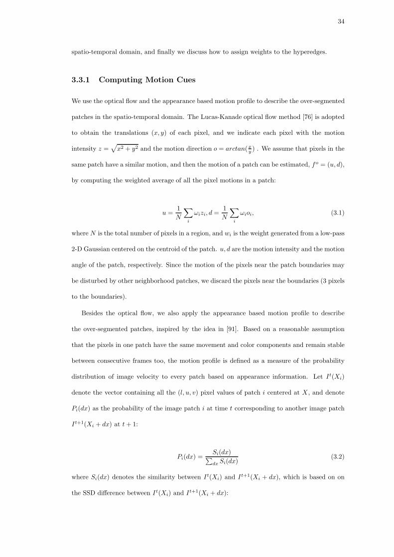
34
spatio-temporal domain, and finally we discuss how to assign weights to the hyperedges.
3.3.1 Computing Motion Cues
We use the optical flow and the appearance based motion profile to describe the over-segmented
patches in the spatio-temporal domain. The Lucas-Kanade optical flow method [76] is adopted
to obtain the translations (x, y) of each pixel, and we indicate each pixel with the motion
intensity z =√
x2 + y2 and the motion direction o = arctan(xy ) . We assume that pixels in the
same patch have a similar motion, and then the motion of a patch can be estimated, fo = (u, d),
by computing the weighted average of all the pixel motions in a patch:
u =1
N
∑
i
ωizi, d =1
N
∑
i
ωioi, (3.1)
where N is the total number of pixels in a region, and wi is the weight generated from a low-pass
2-D Gaussian centered on the centroid of the patch. u, d are the motion intensity and the motion
angle of the patch, respectively. Since the motion of the pixels near the patch boundaries may
be disturbed by other neighborhood patches, we discard the pixels near the boundaries (3 pixels
to the boundaries).
Besides the optical flow, we also apply the appearance based motion profile to describe
the over-segmented patches, inspired by the idea in [91]. Based on a reasonable assumption
that the pixels in one patch have the same movement and color components and remain stable
between consecutive frames too, the motion profile is defined as a measure of the probability
distribution of image velocity to every patch based on appearance information. Let It(Xi)
denote the vector containing all the (l, u, v) pixel values of patch i centered at X , and denote
Pi(dx) as the probability of the image patch i at time t corresponding to another image patch
It+1(Xi + dx) at t + 1:
Pi(dx) =Si(dx)
∑
dx Si(dx)(3.2)
where Si(dx) denotes the similarity between It(Xi) and It+1(Xi + dx), which is based on on
the SSD difference between It(Xi) and It+1(Xi + dx):

35
Si(dx) = exp(−SSD(It(Xi), It+1(Xi + dx))). (3.3)
3.3.2 Spectral Analysis for Hyperedge Computation
The idea of spectral analysis is based on an affinity matrix A, where A(i, j) is the similarity
between sample i and j [93] [81] [109]. Based on the affinity matrix, the Laplacian matrix can
be defined as L = D− 12 (D−A)D− 1
2 , where D is the diagonal matrix D(i, i) =∑
j A(i, j). Then
unsupervised data clustering can be achieved by doing eigenvalue decomposition of the Lapla-
cian matrix. The popular way is to use the k-means method on the first several eigenvectors
associated with the smallest non-zero eigenvalues [81] to get the final clustering result.
To set up the hyperedges, we perform the spectral analysis on the optical flow and the
appearance based motion profile respectively. As in [93] [81] [109], only local neighbors are
taken into account for the similarity computation. We defined two patches to be spatial-temporal
neighbors if 1) in the same frame they are 8-connected or both their centroids fall into a ball of
radius R, or 2) in the adjacent frames (±1 frame in the work) their regions are overlapped or
8-connected, as illustrated in Figure 4.1.
Denote the affinity matrices of the optical flow as Ao and the motion profile as Ap respec-
tively. For the motion profile, we define the similarity between two neighbor patches i and j is
defined as:
Ap(i, j) = e−dis(i,j)
σp , dis(i, j) = 1 −∑
dx
Pi(dx)Pj(dx), (3.4)
where dis(i, j) is defined as the distance between two patches i and j, and σp is constant
computed as the standard deviation of dis(i, j).
Based on the optical flow, the similarity metric between two neighbor patches i and j is
defined as:
Ao(i, j) = e−‖fm
i−fm
j‖2
σo , (3.5)
where σo is a constant computed as the standard deviation of ‖foi − fo
j ‖2.

36
(1) (2)
(3) (4)
Figure 3.3: Four binary partition results got by the first 4 eigenvectors computed from motionprofile (for one frame of the sequence WalkByShop1cor.mpg, CAVIAR database. ).
Based on Ao and Ap, we can compute the corresponding Laplacian matrix of Lo and Lp and
their eigenvectors associated with the first k smallest non-zero eigenvalues respectively. Each of
these eigenvectors may lead to a meaningful but not optimal 2-way cut result. Figure 3.3 shows
some examples, where the patches without the gray mask are regarded as the vertices having the
attribute value 1 and the patches with the gray mask having the attribute 0. A hyperedge can
be formed by those vertices with same attribute values. With all the hyperedges, the complex
relationship between the image patches can be represented by the hypergraph completely.
3.3.3 Hyperedge Weights
According to [93], the eigenvectors of the smallest k non-zero eigenvalues can be used for clus-
tering. Then a nature idea is to choose the first k eigenvectors to compute the hyperedges,
and weight those heyperedges with their corresponding reciprocals of the eigenvalues. In our
experiments, we find that the eigenvalues of the first k eigenvectors are very close and may

37
(1) 0.3506 (2) 0.2403
(3) 0.2378 (4) 0.0986
Figure 3.4: 4 binary partition results with largest hyperedge weights (for one frame of Walk-ByShop1cor.mpg ). Obviously that the heperedge got from the 1st and 4th frames have agood description of objects we want to segment according to their importance. The computedhyperedge weights are shown below those binary images.
not absolutely reflect the importance of the corresponding eigenvectors. In order to emphasize
more important hyperedges which contain moving objects, larger weights should be assigned to
them.
We impose the weights to the hyperedges from two different cues, woH and wp
H , by the
following equations:
woH = co‖fo
1 − fo0‖2 (3.6)
wpH = cpdis(1, 0) (3.7)
where co and cp are constant, and dis(1, 0) means the dissimilarity between two regions in
the binary image with value 1 and 0, based on the first motion feature; fo1 and fo
0 means the
weighted motion intensity and direction of two regions in the binary image with value 1 and 0.

38
Based on above definition, a larger weight is assigned to the binary frame whose two segmented
regions have distinct appearance (motion) distributions.
In practice, we select the first 5 hyperedges with larger weights computed from appear-
ance and motion respectively; and then proper cp and co are chosen to let∑5
i=1 wpH(i) = 1
and∑5
i=1 woH(i) = 1. In 3.4, we show the corresponding weight values under the binary at-
tribute images. It is obvious that more meaningful attributes are assigned larger weights in our
algorithm.
After the construction of hypergraphs for video object segmentation, the theoretical solution
of this real value problem is the eigenvector associated with the smallest non-zeros eigenvector
of the hypergraph Laplacian matrix ∆ = I − D− 1
2v HWD−1
e HT D− 1
2v . As in [81], to make a
multi-way classification of vertices in a hypergraph, we take the first several eigenvectors with
non-zeros eigenvalues of ∆ as the indicators (we take 3 in this work), and then use a k-means
clustering algorithms on the formed eigenspace to get final clustering results.
3.4 Experiments
3.4.1 Experimental Protocol
To evaluate the performance of our segmentation method based on the hypergraph cut, we
compare it with three clustering approaches based on the simple graph, i.e., the conventional
simple graph with pairwise relationship. In these three approaches, we measure the similarity
between two over-segmented patches using (1) the optical flow, (2) the motion profile, and
(3) both the motion cues. The similarity matrix for (1) and (2) just follow Equation 3.5 and
Equation 3.4. For (3), the similarity is defined as follows:
A(i, j) = e−‖fm
i−fm
j‖2
σo −dis(i,j)
σp , (3.8)
where σo and σp are constants. Notice that σ values in Equation 3.8, Equation 3.4 and Equa-
tion 3.5 are all tuned to get the best segmentation results for both the hypergraph based and
the simple graph based methods for comparison. Then corresponding Laplacian matrix of these
three approaches can be computed accordingly and the k-means algorithm can be performed

39
on the first n eigenvectors with nonzero eigenvalues. In our experiment, we choose n = 10 for
all these three simple graph based methods.
3.4.2 Results on Videos under Different Conditions
We first report the experiments on the rocking-horse sequence and the squirrel sequence used
in [97]. We choose them because the movement of objects in these two sequences are very
subtle and their backgrounds are cluttered and similar to the objects. Figure 3.5 and 3.6 show
the ground truth frames, the results of three simple graph based methods, and the results
of hypergraph cut for these two sequences. To illustrate a distinctive comparison with the
ground truth, we plot the red edge of the segmented patches in our results. Compared with the
results in [97] and the simple graph based methods, in both sequences our method gives more
meaningful segmentation results for the foreground objects, although a few local details are lost
in the squirrel sequence. In all these figures, the number of cluster classes is set to 2 (K=2).
We also compare four algorithms on the image sequences in which the video object has com-
plicated movements. The sequence shown in Figure 3.7 (Walk1.mpg, from CAVIAR database)
contains a person browsing back and forth and rotating during the course of his movement. In
this example, we cluster the scene to two classes (K=2) too. From Figure 3.7, we can observe
that our method can give very accurate segmentation result for the moving objects, in spite of
the small perturbation in the left corners of this sequence. However, the simple graph based
methods can not completely extract the moving person from background and some unexpected
small patches are classified into the moving objects.
In the real world, the video objects may be occluded or interacted with each other during
their movements. We also test the proposed method on such examples with occlusion. In
Figure 3.8, four algorithm are compared on a running-car sequence with an artificial occlusion,
in which the hypergraph cut extracts the car and the pedestrian from the background accurately,
while the simple graph based methods can extract the car or the pedestrian. In the sequence
shown in Figure 3.9 (WalkByShop1front.mpg, from CAVIAR database), a couple walk along
the corridor, and another person moves to the door of the shop hastily and is occluded by the
couple during his moving. When we set K=2, the person with largest velocity of movement

40
Sequence Name MP OP MP+OP Hypergraph CutRocking-horse 0.87/0.02 0.96/0.76 0.96/0.92 0.91/0.02
Squirrel 0.91/0.86 0.89/1.32 0.72/0.02 0.89/0.01Walk1 0.92/15.3 0.92/6.4 0.92/12.7761 0.94/0.03
car running 0.14/0.03 0.82/0.02 0.82/3.22 0.89/0.03WalkByShop1front 0.32/0.47 0.56/0.81 0.79/0.66 0.84/0.37
Table 3.1: Average accuracy/error for all the experimental frames of every sequence, whereMP means simple graph method by the motion profile, OP means simple graph method by theoptical flow and MP+OP means the simple graph method using both cues. Mention that forWalkByShop1front.mpg we only consider the case when K=4.
is segmented. When we set K=3, K=4 and K=5, three primary moving objects are extracted
one by one only with a small patch between the couple, which is caused by the noise of motion
estimation. For the simple graph based methods, we give the best case (the best result under
different K). For K > 3, simple graph based methods usually give very cluttered and not
meaningful results. For the simple graph based methods using the motion profile or the optical
flow, K =2 can give the most meaningful results, and K =3 can give a good extraction of the
couple for the simple graph method using both motion cues.
In Table 3.1, the average segmentation accuracy and segmentation error are estimated and
compared on the experimental frames of all the image sequences. The segmentation accuracy
for one frame is defined as the number of ’true positive’ pixels (the true positive area) divided
by the number of the ground truth pixels(the ground truth area). The segmentation error for
one frame is defined as the number of ’false positive’ pixels (the false positive area) divided by
the number of the ground truth pixels(the ground truth area).
3.5 Conclusions
In this chapter, we proposed a framework of video object segmentation , in which hypergraph
is used to represent the complex relationship among frames in videos. We first used the multi-
scale graph decomposition method to over-segment the images and took the oversegmented
image patches as the vertices of the hypergraph. The spectral analysis was performed on
two motion cues respectively to set up the hyperedges, and the spatio-temporal information is
integrated by the hyperedges. Furthermore, a weighting procedure is discussed to put larger
weights on more important hyperedges. In this way, the task of video object segmentation is

41
transferred into a hypergraph partition problem which can be solved by the hypergraph cut
algorithm. The effectiveness of the proposed method is demonstrated by extensive experiments
on nature scenes. Since our algorithm is a open system, in the future work, we may add more
motion or appearance cues (such as texture information, the occlusions between frames) into
our framework to construct more hyperedges and further improve the accuracy of these results.

42
(a) (b)
(c) (d)
(e)
Figure 3.5: Segmentation results for the 8th frame of the rocking-horse sequence. (a) Theground truth, (b) the result by the simple graph based segmentation using optical flow, (c) theresult by the simple graph based segmentation using motion profile, (d) the result by the simplegraph based segmentation using both motion cues, and (e) the result by the hypergraph cut.

43
(a) (b)
(c) (d)
(e)
Figure 3.6: Segmentation results for the 4th frame of the squirrel sequence. (a) The groundtruth, (b) the result by the simple graph based segmentation using optical flow, (c) the resultby the simple graph based segmentation using motion profile, (d) the result by the simple graphbased segmentation using both motion cues, and (e) the result by the hypergraph cut.

44
(a) (b)
(c) (d)
(e)
Figure 3.7: Segmentation results for one frame of Walk1.mpg, CAVIAR database. (a) Theground truth, (b) the result by the simple graph based segmentation using optical flow, (c) theresult by the simple graph based segmentation using motion profile, (d) the result by the simplegraph based segmentation using both motion cues, and (e) the result by the hypergraph cut.

45
(a) (b)
(c) (d)
(e)
Figure 3.8: Segmentation results for the 16th frame of the car running sequence with occlusion.(a) The ground truth, (b) the result by the simple graph based segmentation using optical flow,(c) the result by the simple graph based segmentation using motion profile, (d) the result by thesimple graph based segmentation using both motion cues, and (e) the result by the hypergraphcut.

46
(a) (b)
(c) (d)
(e) (f)
(g) (h)
Figure 3.9: Segmentation results for one frame of the WalkByShop1front.mpg, different colorsdenote different clusters in each sub-figure. (a) The ground truth, (b) the result by the simplegraph based segmentation using optical flow (K=2), (c) the result by the simple graph basedsegmentation using motion profile (K=2), (d) the result by the simple graph based segmentationusing both motion cues (K=3), (e) the result by the hypergraph cut (K=2), (f) the result bythe hypergraph cut (K=3), (g) the result by the hypergraph cut (K=4), and (h) the result bythe hypergraph cut (K=5).

47
Chapter 4
Unsupervised Image Categorization by Hypergraph
Partition
In this chapter, we present a framework for unsupervised image categorization, in which images
containing specific objects are taken as vertices in a hypergraph, and the task of image clustering
is formulated as the problem of hypergraph partition. First, a novel method is proposed to
select the region of interest (ROI) of each image, and then hyperedges are constructed based on
shape and appearance features extracted from the ROIs. Each vertex (image) and its k-nearest
neighbors (based on shape or appearance descriptors) form two kinds of hyperedges. The weight
of a hyperedge is computed as the sum of the pairwise affinities within the hyperedge. Through
all the hyperedges, not only the local grouping relationships among the images are described, but
also the merits of the shape and appearance characteristics are integrated together to enhance
the clustering performance. We use the generalized spectral clustering technique to solve the
hypergraph partition problem. We compare the proposed method to several methods and its
effectiveness is demonstrated by extensive experiments on three image databases.
4.1 Introduction
Unsupervised image categorization based on some similarity measurements is a critical prepro-
cessing step in many computer vision problems. Supervised approaches (such as SVM, boosting,
etc.) of object detection and recognition typically require a lot of training images whose classes
are labelled and/or bounding boxes of the objects of interest are annotated. Generally this
training data is manually selected and annotated, which is expensive to obtain and may intro-
duce bias information into the training stage. An unsupervised technique (such as k -centers
clustering [79] and affinity propagation based clustering [39] etc) bases its categorization de-
cision directly on the data. It not only recovers image categories naturally, but also provides

48
a powerful tool to collect exemplar images for learning based applications. For unsupervised
image categorization, topic model based clustering has been demonstrated to outperform clas-
sical methods such as k-means by extensive experiments [94] [70] [85]. [34] and [72] extend the
topic models with spatial information to boost categorization results. Topic models can also be
combined with image segmentation information [88] or with a hierarchical class structure [95].
In [101], a complicated model based on tree matching is proposed for unsupervised discover of
topic hierarchies. Other works, such as [40] and [84], try to discover object classes and locations
by detecting reoccurring structure or frequent features sets. [59] presents an iterative method
to amplify ‘consistency’ existing in objects of the same class, by using a novel star-like geomet-
ric model and an appearance learning tool. This unsupervised algorithm leads to precise part
localization and classification performance comparable to supervised approaches, but mainly for
class vs. non-class mixes (i.e. sets formed by some images of one specific class and some other
non-class images). Recent related works include organizing images into a tree shaped hierarchy
by a Bayesian model [46] and discovering object shapes from unlabeled images [68], etc.
Different from the above methods, recently Grauman et al. [44] and Kim et al. [62] [63]
adopt the pairwise graph (for simplicity, we denote the pairwise graph as simple graph in
the following) to model relationship between unlabeled images. These works differ in how
to measure the similarities between images: in [44], image-to-image affinities are computed by
pyramid matching kernel (PMK) [43]; while in [62] and [63], the distance metric between images
is based on link analysis techniques, which largely improves the object detection/categorization
performance on some classes of Caltech-101 [69]. [80] encodes object similarity and spatial
context between object exemplars into simple graphs with two kinds of pairwise edges. Spectral
clustering [81] is usually utilized to solve the simple graph based partitioning problem [43] [62]
and its superiority over previous methods is verified in [103].
To overcome the limitations of simple graph based methods mentioned above, we propose
a hypergraph based framework to exploit the correlation information among unlabeled images
containing distinct objects, and adopt a hypergraph partition algorithm to improve unsupervised
image categorization performance. Different from simple graph, hypergraph contains summa-
rized local grouping information, which may be beneficial to the global clustering. Moreover,

49
Figure 4.1: Illustration of our framework.
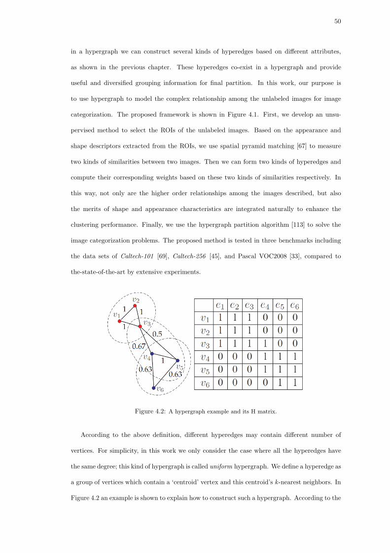
50
in a hypergraph we can construct several kinds of hyperedges based on different attributes,
as shown in the previous chapter. These hyperedges co-exist in a hypergraph and provide
useful and diversified grouping information for final partition. In this work, our purpose is
to use hypergraph to model the complex relationship among the unlabeled images for image
categorization. The proposed framework is shown in Figure 4.1. First, we develop an unsu-
pervised method to select the ROIs of the unlabeled images. Based on the appearance and
shape descriptors extracted from the ROIs, we use spatial pyramid matching [67] to measure
two kinds of similarities between two images. Then we can form two kinds of hyperedges and
compute their corresponding weights based on these two kinds of similarities respectively. In
this way, not only are the higher order relationships among the images described, but also
the merits of shape and appearance characteristics are integrated naturally to enhance the
clustering performance. Finally, we use the hypergraph partition algorithm [113] to solve the
image categorization problems. The proposed method is tested in three benchmarks including
the data sets of Caltech-101 [69], Caltech-256 [45], and Pascal VOC2008 [33], compared to
the-state-of-the-art by extensive experiments.
Figure 4.2: A hypergraph example and its H matrix.
According to the above definition, different hyperedges may contain different number of
vertices. For simplicity, in this work we only consider the case where all the hyperedges have
the same degree; this kind of hypergraph is called uniform hypergraph. We define a hyperedge as
a group of vertices which contain a ‘centroid’ vertex and this centroid’s k -nearest neighbors. In
Figure 4.2 an example is shown to explain how to construct such a hypergraph. According to the

51
similarities on the pairwise edges, each vertex and its two-nearest neighbors form a hyperedge.
In Figure 4.2, hyperedges are marked by ellipses. For example, the hyperedge e4 is composed of
vertex v4 and its two nearest neighbors v3 and v5. The corresponding vertex-hyperedge matrix
H could be formed as in the right side of Fig. 4.2.
In order to bipartition this hypergraph, intuitively the hyperedges with the smallest weights
should be removed, and at the same time as many hyperedges with larger weights as possible
should be kept. Since e4 has the smallest hyperedge weight, a hypergraph partition could be
made on it to classify v1, v2, ..., v6 into two groups. This is exactly the result obtained by the
normalized hypergraph partition.
4.2 Our Two-Step Method for Unsupervised ROI Detection
Besides cluttered background, various positions and scales of interesting objects in images also
make it unreliable to measure the similarities based on whole images. To overcome this problem,
previous works [12] [22] proposed to extract rectangle ROIs of object instances based on iterative
conditional model [8]. However, they are based on the assumption that the categorization
information of images is known, so they can not work when no prior information (such as the
class labels of objects) is provided. In this work, we propose a novel two-step method to detect
the ROIs from the unlabeled images.
Consider an image set S that contains not only images from one or several object classes,
but also other non-class images. At first we go over the entire set S to compute every image’s
k–nearest neighbors (KNN). We use a KNN algorithm based on vantage point trees, which is
able to provide the best performance for computer vision applications and speed up the search
effectively [64]. To measure the degree of closeness between each image with its neighbors, we
get scores by summing up the distances between each image with its five nearest neighbors.
We sort all the images in S by these scores. Then bottom 5% images with lowest scores are
selected from S and taken as the initial exemplars for the given query. Our object annotation
approach alternates between Rough Localization Phase and accurate ROI localization,
with a continuous expansion of the exemplar set. In this manner the process not only exploits

52
ROI localization results at a given stage to guide the next stage, but also identifies more high-
likelihood images as exemplars related to the input query.
4.2.1 Rough Localization Phase
Initialization is a crucial step in many optimization tasks. A bad initialization may lead to a
local maximum or minimum which is far from the satisfactory solution. In this subsection we
propose efficient initialization procedures to predict the ROI s of the exemplar images. For the
initial exemplars, we create a novel feature weighting framework to divide the foreground and
background; for the new incoming exemplars in the subsequential loops, rough ROI s are found
by a query-by-example technique.
Rough Localization for initial exemplars. The dense SURF features are extracted ev-
ery 12 pixels from three pyramid scales of all the images and a 2000–bins codebook is organized
by k–means algorithm. For each image, we assume that some codewords (bins) in the codebook
are more relevant to the foreground objects while some other codewords are more relevant to
the background. Taking each initial exemplar as the centroid, we collect its npos = 3% × N
nearest neighbors as the positive set (where N is the total number of the unlabelled images); we
randomly sample nneg = 10% × N images from the top 30% farthest neighbors as the negative
set. Intuitively, foreground features should have more contribution to the similarity between
the centroid image and the images in the positive set; the similarity between the centroid image
and the images in the negative set is caused by false matches in some bins. For each code-
word, we accumulate the pairwise intersection between the histogram (on the level l = 0) of the
centroid image and the histograms of the images from the positive/ negative set respectively.
After normalization, we can obtain two density functions DESposi (w) and DESneg
i (w) for the
exemplar image i, which describe the overall distributions of matches on two image sets:
DESposi (w) =
∑
j∈Pi
min(Hisi0(w), Hisj
0(w))
∑|V |k=1 DESpos
i (vk), (4.1)
DESnegi (w) =
∑
j∈Ni
min(Hisi0(w), Hisj
0(w))
∑|V |k=1 DESneg
i (vk). (4.2)
where Pi and Ni are the positive set and the negative set for the exemplar i, respectively.

53
For simplicity, we denote these two density functions as the positive and negative distributions
respectively. The value of DESposi (w) − DESneg
i (w) reveals to what extend a codeword w is
related to the foreground objects or the background. Since every SURF feature is quantized
into a histogram by soft assignment according to Eq. 5.10, we can assign weights to all SURF
features based on these two distributions:
weighti(f) =
∑|V |j=1[DESpos
i (vj) − DESnegi (vj)]Kσ(D(vj , f))
∑|V |j=1 Kσ(D(vj , f))
(4.3)
where weighti(f) is the weight of the SURF feature f in the exemplar image i. According to
the above analysis, localizing the ROIs roughly is equivalent to finding a rectangular region R
in the centroid image to maximize the sum of all the feature weights:
argmaxR∈R
∑
∀f∈R
weight(f) = arg maxR∈R
F+(R) + F−(R) (4.4)
where R is the set of all possible rectangles in the image, F+(R) and F−(R) are the sum of all
the positive weights and the sum of all the negative weights in R, respectively. To solve Eq. 4.6,
traditional methods need to exhaustively search all the possible windows in the image. In this
work, we adopt a ‘beyond sliding windows’ scheme [65] to obtain the optimal solution of Eq. 4.6
in typically sublinear time. The details are shown in Algorithm 1.
Algorithm 1 Learning the rough ROIs of initial exemplars
1: for each image i: do2: collect its positive set Pi and its negative set Ni based on the spatial pyramid matching
algorithm [67];3: accumulate and normalize the intersection scores between the exemplar image i and the
images in the positive set Pi, from codeword to codeword, according to Eq. 4.1;4: accumulate and normalize the intersection scores between the exemplar image i and the
images in the negative set Ni, from codeword to codeword, according to Eq. 4.2;5: compute the weight for each feature according to Eq. 4.3;6: obtain the rough ROI of the exemplar image i by maximizing Eq. 4.6 by the ‘beyond
sliding windows’ [65] method.7: end for
Rough Localization for subsequent exemplars. The rough ROI localization results in
initial exemplars can be refined with the method introduced in Section 4.2. Then those refined
ROI s in the current exemplar set are used as query examples to search for their most similar
subregions in all the non-exemplar images. In [65], the ‘beyond sliding windows’ method is
also employed to search for similar subregions efficiently in multiple images. For simplicity,

54
we only search each ROI ’s most similar subregion from non-exemplar images, add that image
to the exemplar set and take the subregion as its rough ROI. The new exemplar is taken as
the ‘child’ of the query exemplar. If a new incoming exemplar has two ore more ancestors,
the rough ROI it contained is the most similar subregion to all its ancestors. Similar to those
initial exemplars, the positive and negative set of every new exemplar will be prepared for the
accurate ROI localization phase.
4.2.2 Accurate ROI Localization
After obtaining the rough ROI locations in all images of the current exemplar set, we need to
refine them and obtain the final ROIs by maximizing the following cost function:
|E|∑
i=1
−∑
j∈Pi
DIS(i, j) +∑
k∈Ni
DIS(i, k) (4.5)
where |E| is the number of images in the current exemplar set; Pi and Ni are the positive set
and the negative set for the exemplar i, respectively. DIS is the distance function based on
the shape descriptors and the appearance descriptors, which are computed according to Eq. ??.
In Eq. 4.5, we try to optimize the ROI of each exemplar by minimizing the distance between
each exemplar and its positive set, while simultaneously maximizing the distance between each
exemplar and its negative set. It is very expensive to optimize Eq. 4.5 exhaustively. To overcome
this problem, We adopt a sub-optimal scheme based on the iterative conditional model(ICM) [8],
which is used in previous works [12] [22]. We first enlarge the rough ROIs by 15% and search
refined ROIs in this enlarged range using several window sizes(we obtain search window sizes
by extending and shrinking the width or(and) the length of a rough ROI by 5% and 10%). To
reach this goal, we define the following function and maximize it:
L(R1,...,R|V |)=
|V |∑
i=1
∑
j∈Pi
(Asi,j+Aa
i,j)−∑
k∈Ni
(Asi,k+Aa
i,k), (4.6)
where |V | is the number of all the images; Asi,j is the abbreviation of As(Ri, Rj), Ri is the ROI
candidate of the ith image; Pi and Ni are the positive set and negative set of the ith image,
respectively; As and Aa are two different affinity functions based on the appearance descriptor
and the shape descriptor respectively to measure the similarities between two ROI candidates.
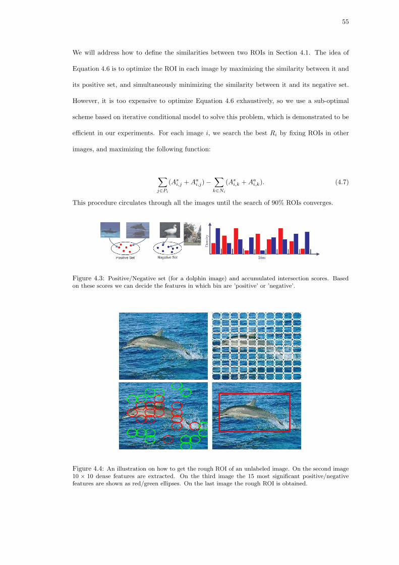
55
We will address how to define the similarities between two ROIs in Section 4.1. The idea of
Equation 4.6 is to optimize the ROI in each image by maximizing the similarity between it and
its positive set, and simultaneously minimizing the similarity between it and its negative set.
However, it is too expensive to optimize Equation 4.6 exhaustively, so we use a sub-optimal
scheme based on iterative conditional model to solve this problem, which is demonstrated to be
efficient in our experiments. For each image i, we search the best Ri by fixing ROIs in other
images, and maximizing the following function:
∑
j∈Pi
(Asi,j + Aa
i,j) −∑
k∈Ni
(Asi,k + Aa
i,k). (4.7)
This procedure circulates through all the images until the search of 90% ROIs converges.
Figure 4.3: Positive/Negative set (for a dolphin image) and accumulated intersection scores. Basedon these scores we can decide the features in which bin are ’positive’ or ’negative’.
Figure 4.4: An illustration on how to get the rough ROI of an unlabeled image. On the second image10 × 10 dense features are extracted. On the third image the 15 most significant positive/negativefeatures are shown as red/green ellipses. On the last image the rough ROI is obtained.

56
4.3 Hypergraph Partition for Image Categorization
4.3.1 Similarity Measurements Between the ROIs
As mentioned above, we represent each image by the features extracted from its ROI, and the
hyperedge defined in the proposed hypergraph is formed by an image and its k -nearest neighbor.
Therefore, how to define the similarity measurement between the ROIs is a key issue to build the
hypergraph, besides the issue of ROI refinement addressed in the last Section. In this work, we
utilize two kinds of feature descriptors on the ROIs, i.e., the SURF based appearance feature
descriptor and the PHOG (the pyramid histograms of edge oriented gradients) based shape
feature descriptor [28] [13]. Based on these two features we obtain two different similarities,
i.e., As and Aa in Equation 4.7 respectively. We use the speed up robust feature (SURF) as
the appearance descriptor [6] because it approximates or even outperforms previously proposed
local appearance features such as the SIFT [75], and it can be computed much faster. PHOG
is known as a good descriptor to capture shape information.
As shown in Figure 4.5, the SURF features are densely sampled at three scales. Given a
ROI, we densely extract SURF features from 15 × 15 rectangular grids of the ROIs. For those
very small ROIs, we double their sizes to extract the features. We create a 128-bin codebook
of SURF features by k–means, and totally 225 features are quantized into a histogram by soft
assignment as in [106], because such soft assignment technique was proven to make remarkable
improvement in object recognition [106]. For the PHOG descriptor, in each image grid we
discretize it into 20 bins (that is, the length of each ‘bin’ is 360/20 = 18 degree). Since 3
pyramid levels (the grid configurations are 1X1, 2X2, 4X4) are used, so there are actually 420
bins in a PHOG based histogram.
We adopt the spatial pyramid matching(SPM) [67] (illustrated in Figure 4.5) to calculate
the similarities because of its better performance when image ROIs are obtained. Given the
local histograms Hisli and Hisl
j at each level of two images i and j based on the appearance or
shape features, the similarity is computed using a kernel function as follows:
A(Ri, Rj) = exp − 1
β
L∑
l=0
1
2L−ldis(Hisl
i, Hislj), (4.8)

57
where β is the standard deviation of∑
l∈L
12L−l dis(Hisl
i, Hislj) over all the data; dis is the distance
function computed with an improved pyramid matching kernel (PMK) algorithm [43] [44]. In
this work, we set L = 2, as shown in Figure 4.5.
Figure 4.5: From left to right: levels l = 0 to l = 2 of the spatial pyramid grids for theappearance and shape descriptors.
4.3.2 Computation of the Hyperedges
In this work, we take each image as a centroid and collect its k -nearest neighbors by the
shape and appearance descriptors respectively. Then two kinds of hyperedges (based on the
shape/apperance descriptors) can be constructed over these K + 1 images with different hyper-
edge weights. The hyperedge weight w(e) is computed as follows:
w(e) =∑
vi,vj∈ei<j
Ai,j , (4.9)
where the affinity function Ai,j is computed according to Equation4.8. If a hyperedge is con-
structed by the appearance descriptor, the w(e) is computed by Aa. The w(e) is computed by
As when the shape descriptor is used.
For practical hypergraph partition problems, the choice of hyperedge size is crucial to the
final clustering results. Except for the hyperedge size, all the parameters in our framework
are computed from the experimental data directly. Intuitively, very small-size hyperedges only
contain ‘micro-local’ grouping information which will not help the global clustering over all the
images, and very large-size hyperedges may contain images from different classes and suppress
the diversity information. To optimize the clustering results, it is necessary to perform a sweep
over all the possible values of the hyperedge size. In Section 5.2, a sensitivity analysis is made
to investigate the robustness of our algorithm by illustrating how the clustering accuracy varies

58
along with the hyperedge size.
4.3.3 Hypergraph Partition Algorithm
In this work, we adopt the algorithm proposed in [113] to partition the hypergraph because of
its efficiency and simplicity of implementation. As in [81], to make a multi-way classification
of vertices in a hypergraph, we take the first several eigenvectors with non-zero eigenvalues of
the hypergraph Laplacian matrix ∆ as the indicators (we take 3 in this work), and then use a
k-means clustering algorithm on the formed eigenspace to get final clustering results.
4.4 Experiments
4.4.1 Experimental Protocol
In the following, we first make a sensitivity analysis to show the robustness of our algorithm
when the hyperedge size varies. Then we compare our results to the-state-of-the-art [62] on
the same data sets using the same testing protocol. We also compare our method with three
different unsupervised methods: 1. the k -centers clustering [79], 2. the affinity propagation [39],
3. the simple graph based normalized cut. We test these methods and our proposed method on
three different data sets, which are Caltech-101 [69], Caltech-256 [45], and Pascal VOC2008 [33]
respectively. For above three clustering methods, the affinity between two images is defined as
Av = As + Aa based on the features in the selected ROIs. For the simple graph based method,
we build the simple graph by connecting each vertex (image) with its k -nearest neighbors by
pairwise edges. The affinity matrix is constructed as W (i, j) = Avi,j if two vertices are connected
and W (i, j) = 0 otherwise. The spectral analysis is employed to solve an eigen-decomposition
problem, and the first several (we use 3 in this work) eigenvectors are fed to k -means algorithm to
get the final classification results. In our experiments the number of obtained clusters are set the
same as the number of true classes. To evaluate how well the unlabeled images are clustered
according to their ground truth labels, we follow the measurement used in [44] and [62] by
computing the average accuracies over all classes. The image ROI prediction error is defined as
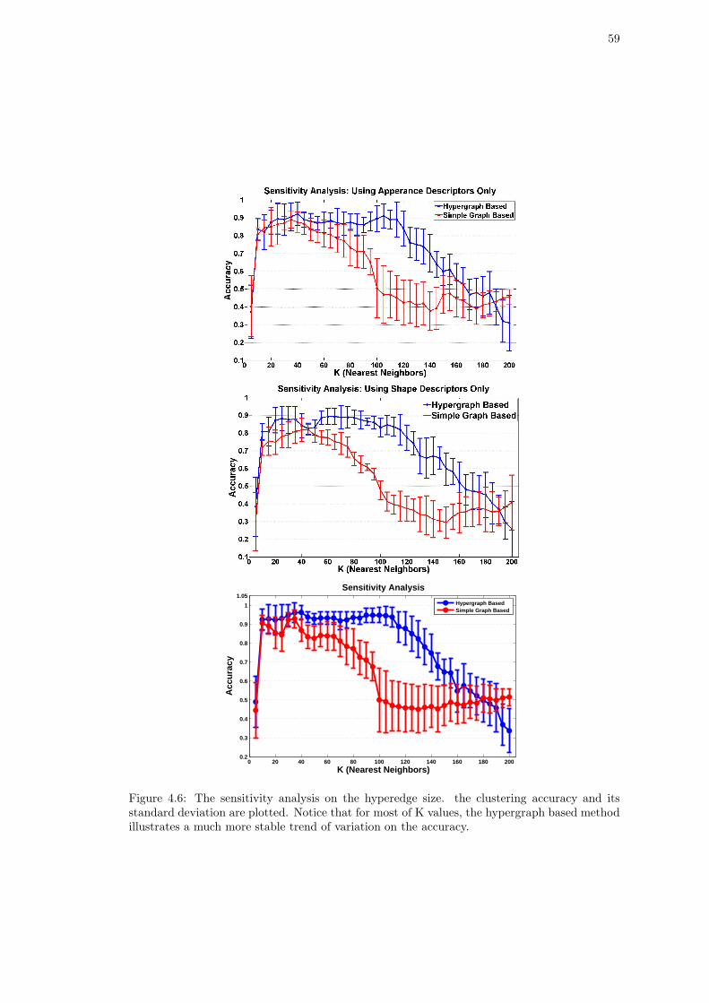
59
0 20 40 60 80 100 120 140 160 180 2000.2
0.3
0.4
0.5
0.6
0.7
0.8
0.9
1
1.05
K (Nearest Neighbors)
Acc
urac
y
Sensitivity Analysis
Hypergraph BasedSimple Graph Based
Figure 4.6: The sensitivity analysis on the hyperedge size. the clustering accuracy and itsstandard deviation are plotted. Notice that for most of K values, the hypergraph based methodillustrates a much more stable trend of variation on the accuracy.

60
Figure 4.7: An illustration for several definitions used in Eq. 4.10.
errloc =0.5 × (FPA + FNA)
FPA + FNA + TPA, (4.10)
where TPA denotes true positive area; FPA denotes false positive area and FNA denotes false
negative area, as shown in Fig. 4.7. Eq. 4.10 can be used as a good single-value measurement
for object localization since a small localization error guarantees small false positive and small
false negative areas at the same time.
4.4.2 Sensitivity Analysis of the Hyperedge Size
Since both the hyperedges in the hypergraph and the edges in the simple graph are formed by
each vertex and its K -nearest neighbors, we report the classification accuracy as a function of
K. To obtain an indication of significance, the bootstrap method [9] is used to estimate the con-
fidence intervals for classification accuracy. In this analysis, we provide a pool of 200 unlabeled
images from Caltech-101 (at first 4 classes are randomly selected from Caltech-101, and then 50
images are randomly chosen from each of the 4 classes). For each K value plotted, we run both
the hypergraph method and the simple graph method 50 times, each time with a different ran-
dom subset of 4 classes. We performe the sensitivity analysis under three circumstances: using
appearance descriptors, using shape descriptors and using both descriptors(if one descriptor is
used, we only use As or Aa as the similarity measure in a simple/hypergraph). In Figure 4.6
the average accuracy and the standard deviation over 50 runs are reported for each K value.
As illustrated in Figure 4.6, the hypergraph based clustering not only obtains better clustering

61
accuracies on most of K values, but also illustrates a much more stable trend of variation on
the accuracy as K increases, especially when 20 < K < 100. By contrast, the simple graph
based clustering shows a lower robustness of the performance on the selection of the parameter
K. In the comparison of the following experiments, we will show the best accuracy of both two
methods by tuning K value.
Here we give an intuitive explanation for why performance of hypergraph models in Fig-
ure 4.6 is still high when K = 100 are used in the hypergraphs. Consider that we transfer
a hypergraph into an equivalent simple graph by Clique Expansion. The pairwise similarity
between two vertices is proportional to the sum of their corresponding hyperedge weights. That
is, in the obtained simple graph, the edge weight between two vertices vi and vj is not decided
by the pairwise affinity Ai,j between two vertices, but the averaged neighboring affinities close
to them; furthermore, this edge weight is influenced more by those pairwise affinities whose two
incident vertices share more hyperedges with vi and vj . In this way the adverse impact caused
by some ’noise’ similarities may be weakened by this weighted averaging or smoothing effect of
the hypergraph construction, even when K is relatively large.
4.4.3 Results on Caltech Data Sets
Compared to [62]. [62] is the latest work on unsupervised image categorization, and it is
based on simple graph partition. So we first compare to this work under the same experiment
setting to show the effectiveness of our framework. Following the approach in [62], we select
six object classes (airplane, motorbikes, rear cars, faces, watches, ketches) from Caltech-101 to
the proposed hypergraph method. For ROI localization results, we report the average errloc
and its standard deviation (std) in Table 4.1 according to Eq. 4.10. The ROI detection results
shown in Table 4.1 is desirable, since objects in images of Caltech-101 are roughly aligned and
backgrounds in those images are relatively simple. For categorization results, Table 4.2 shows
the confusion matrices with increasing number of classes (from four to six). Each experiment
is iterated ten times as in [62], in which 100 images per object are randomly picked from each
object class. As illustrated in Table 4.2, our clustering result for four object classes(98.53%)
is comparable to [62] (98.55%). In the cases of five and six object classes, our results achieve

62
A M C F W K
Error 8.1 5.2 6.8 4.7 9.6 5.5STD 7.6 4.3 5.7 8.2 6.9 7.5
Table 4.1: Average localization errors and standard deviations, computed using Eq. 4.10.A:Airplanes, C: Cars, F: Faces, M: Motorbikes, W: Watches, K: Ketches)
97.38% and 96.05%, which are slightly better than [62] (97.30% and 95.42%). Average cluster-
ing accuracies/std errors are computed using the diagonal entries in corresponding confusion
matrices.
More results on Caltech Data Sets. To further evaluate the performance of our model,
we design a more universal and difficult experiment setting for comparison, which is rarely used
in previous work. We use all image classes from Caltech-101 and Caltech-256 respectively, and
then randomly choose 4, 8, or 12 classes to run 4-category clustering, 8-category clustering or
12-category clustering tasks. In each task, we run the experiment for 100 times to obtain the
average accuracy and the standard deviation. Before each run 4, 8 or 12 image classes are
randomly selected, and then 50 images are randomly chosen from each class to form a pool of
images (for the class in which total number of images is less than 50, all the images in this class
will be used). For the clustering results, as shown in Table 4.3, the hypergraph based method
excels the other three methods on both Caltech-101 and Caltech-256 data sets.
4.4.4 Results on the PASCAL VOC2008
We also test the proposed method on PASCAL VOC2008 database [33]. Unlike Caltech databases,
PASCAL VOC2008 is much more challenging for its class variations and cluttered backgrounds.
To decrease the difficulty, we choose around 800 images from six easier classes (person, aero-
plane, train, boat, moto-bike, and horse) of the VOC2008 for our experimental comparison.
Since in the VOC2008 one image may contain multiple objects, we classify each image to one
specific class according to the most significant object it contains. Same as above, we increase
object classes from 4 to 6 for the clustering tasks. Each experiment is iterated for 50 times, in
which 100 images per object are randomly picked from each object class. In Fig. 4.9, the first
three images are examples with accurate ROI detection results. We also show some difficult
cases in Fig. 4.9: the detection bounding boxes of the 4th and 5th images are not well located,

63
A M C F
A 99.5/0.9 0.0 0.5/0.9 0.0M 0.0 97.9/0.4 2.0/0.5 0.1/0.3C 1.2/0.8 0.1/0.2 98.3/1.1 0.4/0.4F 1.1/1.2 0.3/0.5 0.2/0.3 98.4/1.3
A M C F W
A 98.9/1.7 0.1/0.2 0.6/0.6 0.1/0.3 0.3/0.4M 0.5/0.7 97.8/0.9 1.6/1.0 0.0 0.1/0.2C 1.6/1.5 0.2/0.4 97.5/1.6 0.6/1.1 0.1/0.3F 0.8/1.3 0.4/0.4 0.6/0.5 96.9/1.4 1.3/1.6W 2.1/1.7 0.7/0.9 0.1/0.1 1.4/1.2 95.7/1.3
A M C F W K
A 97.3/3.0 0.2/0.3 0.3/0.5 0.1/0.3 0.1/0.2 2.0/1.8M 0.4/0.7 94.5/2.9 1.4/1.1 0.2/0.2 0.4/0.3 3.1/3.4C 0.9/0.6 0.2/0.4 97.6/2.1 0.1/0.3 0 1.2/1.5F 1.0/0.8 0.4/0.8 0.1/0.4 96.1/2.5 0.9/1.3 1.5/1.8W 1.9/1.7 0.2/0.3 0.1/0.2 0.1/0.1 94.6/3.9 3.1/3.5K 2.2/1.6 0.2/0.4 0.3/0.5 0.4/0.2 0.7/0.9 96.2/2.4
Number of Classes 4 5 6
Our method 98.53/0.93 97.38/1.38 96.05/2.80[62] 98.55/0.98 97.30/1.44 95.42/2.87
Table 4.2: The first three tables are confusion matrix for increasing number of Caltech-101objects from four to six. The average accuracies (%) and the standard deviations (%) areshown in the tables. Comparison to [62] is reported in the last table. The numbers in this tableare computed from the diagonals of first three tables.
because of cluttered background or similar objects shown in the same image. In the 6th image,
the detected ROI is misplaced because of the misleading texture in the background. As shown
in Table 4.4(Above), we obtain higher average ROI localization errors on Pascal database, com-
pared to the results on Caltech (Table 4.1). This affects the image categorization results shown
in Table 4.4(Bottom), which are not as good as the categorization results on Caltech (Table 4.2
and Table 4.3). However, based on the same ROI results, we can still see that the proposed
hypergraph partition method outperforms the other three methods for the image categorization
task.
4.5 Conclusion
In this section, we have presented a hypergraph based framework for unsupervised image cate-
gorization. We first use a new method to extract the ROIs from the unlabeled images, and then
construct hyperedges among images based on shape and appearance features in their ROIs.
The hyperedges are defined as a group formed by each vertex and its k -nearest neighbors, and
their weights are calculated by the sums of the pairwise affinities. Different from the simple

64
Dataset Caltech 101 Caltech 256
Image Classes 4 8 12 4 8 12
Hypergraph Based95.8 86.2 71.5 87.7 77.1 64.3
3.3 4.4 6.8 4.6 6.7 7.0
Simple Graph Based92.8 82.1 66.2 77.9 72.5 59.04.0 6.2 7.1 5.7 7.6 8.5
Affinity Propagation76.1 62.5 54.1 69.7 57.2 51.45.7 6.8 7.6 7.7 6.6 9.1
k -center72.6 56.9 47.9 67.8 53.7 50.25.1 6.5 9.6 8.0 7.5 9.9
Table 4.3: Results of unsupervised image categorization on both Caltech-101 and Caltech-256.
P A T B M H
Error 17.2 9.8 16.3 21.6 7.9 13.8STD 10.8 6.7 5.4 15.4 8.1 6.7
Dataset PASCAL VOC2008
Image Classes 4 5 6
Hypergraph Based81.3 77.2 69.3
3.4 4.6 6.5
Simple Graph Based74.9 71.3 63.74.1 5.2 6.1
Affinity Propagation62.7 57.3 47.94.7 6.4 7.0
k -center58.9 53.6 41.25.3 5.1 5.9
Table 4.4: The first table: average localization errors and standard deviations of the VOC2008,computed using Eq. 4.10. (P:person, A: Aeroplane, T: Train, B:Boat, M: moto-bike, H: Horse).The second table: results of unsupervised image categorization on PASCAL VOC2008. 4-classcase: P,A,T,B. 5-class case: P,A,T,B,M.
graph, the hypergraph not only represents the higher order relationships between the images,
but also efficiently integrates different visual feature descriptors together. We formulate the
image clustering as the problem of hypergraph partition and solve it with a generalized spec-
tral clustering technique. The effectiveness of the proposed method has been demonstrated by
extensive experiments on various database.
Figure 4.8: ROI detection results. The red bounding boxes are the ROI detection results andthe blue boxes are the ground truths. In the first three images very good detection results areobtained. We also give three examples in which ROIs are not well detected.

65
Figure 4.9: ROI detection results. The first two rows are images from Caltech 256; the last tworows are images from PASCAL VOC2008.

66
Chapter 5
Image Retrieval via Fuzzy Hypergraph Ranking
In this chapter, we propose a new transductive learning framework for image retrieval, in which
images are taken as vertices in a weighted hypergraph and the task of image search is formu-
lated as the problem of hypergraph ranking. Based on the similarity matrix computed from
various feature descriptors, we take each image as a ‘centroid’ vertex and form a hyperedge by a
centroid and its k-nearest neighbors. To further exploit the correlation information among im-
ages, we propose a probabilistic hypergraph, which assigns each vertex vi to a hyperedge ej in a
probabilistic way. In the incidence structure of a probabilistic hypergraph, we describe both the
local grouping information and the affinity relationship between vertices within each hyperedge.
After feedback images are provided, our retrieval system ranks image labels by a transductive
inference approach, which tends to assign the same label to vertices that share many incidental
hyperedges, with the constraints that predicted labels of feedback images should be similar to
their initial labels. We compare the proposed method to several other methods and its effec-
tiveness is demonstrated by extensive experiments on Corel5K, the Scene dataset and Caltech
101.
Figure 5.1: Left: A simple graph of six points in 2-D space. Pairwise distances (Dis(i, j))between vi and its 2 nearest neighbors are marked on the corresponding edges. Middle: Ahypergraph is built, in which each vertex and its 2 nearest neighbors form a hyperedge. Right:The H matrix of the probability hypergraph shown above. The entry (vi, ej) is set to the affinity
A(j, i) if a hyperedge ej contains vi, or 0 otherwise. Here A(i, j) = exp(−Dis(i,j)
D), where D is
the average distance.

67
5.1 Introduction
In content-based image retrieval (CBIR) visual information instead of keywords is used to search
images in large image databases. Typically in a CBIR system a query image is provided by
the user and the closest images are returned according to a decision rule. In order to learn a
better representation of the query concept, a lot of CBIR frameworks make use of an online
learning technique called relevance feedback (RF) [87] [51]: users are asked to label images
in the returned results as ‘relevant’ and/or ‘not relevant’, and then the search procedure is
repeated with the new information. Previous work on relevance feedback often aims at learn-
ing discriminative models to classify the relevant and irrelevant images, such as, RF methods
based on support vector machines (SVM) [102], decision trees [78], boosting [100], Bayesian
classifiers [26], and graph-cut [89]. Because the user-labeled images are far from sufficient for
supervised learning methods in a CBIR system, recent work in this category attempts to ap-
ply transductive or semi-supervised learning to image retrieval. For example, [54] presents an
active learning framework, in which a fusion of semi-supervised techniques (based on Gaussian
fields and harmonic functions [115]) and SVM are comprised. In [50] and [49], a pairwise graph
based manifold ranking algorithm [112] is adopted to build an image retrieval system. Cai et
al. put forward semi-supervised discriminant analysis [16] and active subspace learning [15] to
relevance feedback based image retrieval. The common ground of [89], [54], [50] and [16] is that
they all use a pairwise graph to model relationship between images. In a simple graph both
labeled and unlabeled images are taken as vertices; two similar images are connected by an
edge and the edge weight is computed as image-to-image affinities. Depending on the affinity
relationship of a simple graph, semi-supervised learning techniques could be utilized to boost
the image retrieval performance.
In this chapter, we propose a hypergraph based transductive algorithm to the field of image
retrieval. As in the previous chapter, we take each image as a ‘centroid’ vertex and form a
hyperedge by a centroid and its k-nearest neighbors, based on the similarity matrix computed
from various feature descriptors. To further exploit the correlation information among images,
we propose a novel hypergraph model called the probabilistic hypergraph, which presents not
only whether a vertex vi belongs to a hyperedge ej , but also the probability that vi ∈ ej . In
68
this way, both the local grouping information and the local relationship between vertices within
each hyperedge are described in our model. To improve the performance of content-based image
retrieval, we adopt the hypergraph-based transductive learning algorithm to learn beneficial
information from both labeled and unlabeled data for image ranking. After feedback images
are provided by users or active learning techniques, the hypergraph ranking approach tends to
assign the same label to vertices that share many incidental hyperedges, with the constraints
that predicted labels of feedback images should be similar to their initial labels. We further
design a random strategy to reduce the computational cost of the proposed method and make
it possible for larger scale image retrieval. The effectiveness and superiority of the proposed
method is demonstrated by extensive experiments on Corel5K [32], the Scene dataset [70] and
Caltech-101 [69].
In summary, the contribution of this work is fourfold: (i) we propose a new image retrieval
framework based on transductive learning with hypergraph structure, which considerably im-
proves image search performance; (ii) we propose a probabilistic hypergraph model to exploit
the structure of the data manifold by considering not only the local grouping information, but
also the similarities between vertices in hyperedges; (iii) in this work we conduct an in-depth
comparison between simple graph and hypergraph based transductive learning algorithms in the
application domain of image retrieval, which is also beneficial to other computer vision and ma-
chine learning applications. (IV) we introduce a random strategy to reduce the computational
cost rapidly.
5.2 Probabilistic Hypergraph Model
Let V represent a finite set of vertices and E a family of subsets of V such that⋃
e∈E = V .
G = (V, E, w) is called a hypergraph with the vertex set V and the hyperedge set E, and each
hyperedge e is assigned a positive weight w(e). A hypergraph can be represented by a |V |× |E|
incidence matrix Ht:
ht(vi, ej) =
1, if vi ∈ ej
0, otherwise.
(5.1)

69
The hypergraph model has proven to be beneficial to various clustering and classification
tasks [2] [98] [56] [99]. However, the traditional hypergraph structure defined in Equation 5.1
assigns a vertex vi to a hyperedge ej with a binary decision, i.e., ht(vi, ej) equals 1 or 0. In
this model, all the vertices in a hyperedge are treated equally; relative affinity between vertices
is discarded. This ‘truncation’ processing leads to the loss of some information, which may be
harmful to the hypergraph based applications.
In this work, we propose a probabilistic hypergraph model to overcome this limitation.
Assume that a |V |× |V | affinity matrix A over V is computed based on some measurement and
A(i, j) ∈ [0, 1]. We take each vertex as a ‘centroid’ vertex and form a hyperedge by a centroid
and its k-nearest neighbors. That is, the size of a hyperedge in our framework is k + 1. The
incidence matrix H of a probabilistic hypergraph is defined as follows:
h(vi, ej) =
A(j, i), if vi ∈ ej
0, otherwise.
(5.2)
According to this formulation, a vertex vi is ‘softly’ assigned to ej based on the similarity A(i, j)
between vi and vj , where vj is the centroid of ej . A probabilistic hypergraph presents not only
the local grouping information, but also the probability that a vertex belongs to a hyperedge.
In this way, the correlation information among vertices is more accurately described. Actually,
the representation in Equation 5.1 can be taken as the discretized version of Equation 5.2. The
hyperedge weight w(ei) is computed as follows:
w(ei) =∑
vj∈ei
A(i, j). (5.3)
Based on this definition, the ‘compact’ hyperedge (local group) with higher inner group sim-
ilarities is assigned a higher weight. For a vertex v ∈ V , its degree is defined to be d(v) =
∑
e∈E w(e)h(v, e). For a hyperedge e ∈ E, its degree is defined as δ(e) =∑
v∈e h(v, e). Notice
that these definitions are relaxed from those definition in ordinary hypergraphs. Let us use
Dv,De and W to denote the diagonal matrices of the vertex degrees, the hyperedge degrees and
the hyperedge weights respectively. Figure 5.1 shows an example to explain how to construct a
probabilistic hypergraph.

70
5.3 Hypergraph Ranking Algorithm
Algorithm 2 Probabilistic Hypergraph Ranking
1: Compute similarity matrix A based on various features using Equation 5.13, where A(i, j)denotes the similarity between the ith and the jth vertices.
2: Construct the probabilistic hypergraph G. For each vertex, based on the similarity matrixA, collect its k-nearest neighbors to form a hyperedge.
3: Compute the hypergraph incidence matrix H where h(vi, ej) = A(j, i) if vi ∈ ej andh(vi, ej) = 0 otherwise. The hyperedge weight matrix is computed using Equation 5.3.
4: Compute the hypergraph Laplacian ∆ = I − Θ = I − D− 1
2v HWD−1
e HT D− 1
2v .
5: Given a query vertex and the initial labeling vector y, solve the linear system((1 + µ)I − Θ) f = µy. Rank all the vertices according to their ranking scores in descendingorder.
Algorithm 3 Manifold Ranking
1: Same to Algorithm 1.2: Construct the simple graph Gs. For each vertex, based on the similarity matrix A, connect
it to its k-nearest neighbors.3: Compute the simple graph affinity matrix As where As(i, j) = A(i, j) if the ith and the jth
vertices are connected. Let As(i, i) = 0. Compute the vertex degree matrix D =∑
j As(i, j).
4: Compute the simple graph Laplacian ∆s = I − Θs = I − D− 12 AsD
− 12 .
5: Same to Algorithm 1, expect that Θ is replaced with Θs.
Let’s revisit the hypergraph based transductive learning algorithm. For a hypergraph par-
tition problem, the normalized cost function [113] Ω(f) could be defined as
1
2
∑
e∈E
∑
u,v∈e
w(e)h(u, e)h(v, e)
δ(e)
(
f(u)√
d(u)− f(v)√
d(v)
)2
, (5.4)
where the vector f is the image labels to be learned in our retrieval problem. By minimizing
this cost function, vertices sharing many incidental hyperedges are guaranteed to obtain similar
labels. Defining Θ = D− 1
2v HWD−1
e HT D− 1
2v , we can derive Equation 5.4 as follows:
Ω(f) =∑
e∈E
∑
u,v∈e
w(e)h(u, e)h(v, e)
δ(e)
(
f2(u)
d(u)− f(u)f(v)√
d(u)d(v)
)
=∑
u∈V
f2(u)∑
e∈E
w(e)h(u, e)
d(u)
∑
v∈V
h(v, e)
δ(e)
−∑
e∈E
∑
u,v∈e
f(u)h(u, e)w(e)h(v, e)f(v)√
d(u)d(v)δ(e)
= fT (I − Θ)f, (5.5)
where I is the identity matrix. Above derivation for probabilistic hypergraphs shows that (i)

71
Ω(f, w) = fT (I −Θ)f if and only if∑
v∈V
h(v,e)δ(e) = 1 and
∑
e∈E
w(e)h(u,e)d(u) = 1, which is true because
of the definition of δ(e) and d(u) in Section 2; (ii) ∆ = I − Θ is a positive semi-definite matrix
called the hypergraph Laplacian and Ω(f) = fT ∆f . The above cost function has the similar
formulation to the normalized cost function of a simple graph Gs = (Vs, Es):
Ωs(f) =1
2
∑
vi,vj∈Vs
As(i, j)
(
f(i)√Dii
− f(j)√
Djj
)2
= fT (I − D− 12 AsD
− 12 )f = fT ∆sf, (5.6)
where D is a diagonal matrix with its (i, i)-element equal to the sum of the ith row of the
affinity matrix As; ∆s = I − Θs = I − D− 12 AsD
− 12 is called the simple graph Laplacian. As
shown in previous chapters, in an unsupervised framework Equation 5.4 and Equation 5.6 can
be optimized by the eigenvector related to the smallest nonzero eigenvalue of ∆ and ∆s [113],
respectively.
In the transductive learning setting [113], we define a vector y to introduce the labeling
information of feedback images and to assign their initial labels to the corresponding elements
of y: y(v) = 1|Pos| , if a vertex v is in the positive set Pos, y(v) = − 1
|Neg| , if it is in the negative
set Neg. If v is unlabeled, y(v) = 0. To force the assigned labels to approach the initial labeling
y, a regularization term is defined as follows:
‖f − y‖2 =∑
u∈V
(f(u) − y(u))2. (5.7)
After the feedback information is introduced, the learning task is to minimize the sum of two
cost terms with respect to f [112] [113], which is
Φ(f) = fT ∆f + µ‖f − y‖2, (5.8)
where µ > 0 is the regularization parameter. Differentiating Φ(f) with respect to f , we have
f = (1 − γ)(I − γΘ)−1y, (5.9)
where γ = 11+µ . This is equivalent to solving the linear system ((1 + µ)I − Θ) f = µy.

72
For the simple graph, we can simply replace Θ with Θs to fulfill the transductive learning.
In [50] and [49], this simple graph based transductive reasoning technique is used for image
retrieval with relevance feedback. The procedures of the probabilistic hypergraph ranking al-
gorithm and simple graph based manifold ranking algorithm are listed in Algorithm 2 and
Algorithm 3.
5.4 Random Hypergraph Ranking
As above description, the hypergraph Laplacian matrix ∆ plays an important role in the ranking
algorithm. The dimensionality of the matrix ∆ is N×N , where N is the data size, and it directly
dominates the computational complex of the ranking algorithm. According to Equation 5.9,
we can see the computational complexity increases with the data size at least by N2. Thus,
its efficiency will be degraded in the case of large-scale data. To handle this issue, we adopt
a random strategy to speed up the proposed method, especially for the large-scale data. The
technique of random sampling has widely used in the community of machine learning [53] [108].
The basic idea is to generate multiple subsets of feature or data from the original one by
randomly sampling and to learn multiple classifiers. Finally combining all these classifiers to
make the final decision. Motivated by this idea, we present a scheme of random hypergraph
ranking for image retrieval.
Assuming in the image data X = x1, x2, ...xl is the label images and X ′ = x′1, x
′2, ..., x
′p
is the unlabeled images, l + p = N . The goal of hypergraph ranking is to predict the labels of
X ′ according to the labeled images X by (9). Usually the size of X is small, so we generate
m subset of X ′ by sampling, X ′1, X
′2..., X
′m. We denote the vector S = s1, s2, ..., sp to
index the selected number of each unlabeled image. In our sampling trick, we keep each sample
x′i ∈ X ′ be selected at least one time, i.e., si ≥ 1. We combine X with each X ′
i to generate
a new image set, X∗i = X ∪ X ′
i, and perform the hypergraph ranking algorithm on each X∗i
respectively. Thus, for each unlabeled image x′i, we can obtain si predictions, y1
i , y2i , ..., ysi
i ,
and we finally decide its label by the value of yi = 1si
si∑
j=1
yji . With the help of sampling, we
only need to perform the hypergraph ranking learning on the image set X∗i , which is smaller
than the original set X ∪ X ′, so the computational cost can be reduced rapidly. The detailed

73
performance will be evaluated in the Section of Experiments.
5.5 Feature Descriptors and Similarity Measurements
Figure 5.2: The spatial pyramids for the distance measure based on the appearance descriptors.Three levels of spatial pyramids for the appearance features are: 1 × 1(whole image, l = 0),1 × 3(horizontal bars, l = 1),2 × 2(image quarters, l = 2).
To define the similarity measurement between two images, we utilize the following descrip-
tors: SIFT [75], OpponentSIFT, rgSIFT, C-SIFT, RGB-SIFT [105] and PHOG [28] [13]. The
first five are appearance-based color descriptors that are studied and evaluated in [105]. It
is verified that their combination has the best performance on various image datasets. HOG
(histogram of oriented gradients) is the shape descriptor widely used in object recognition and
image categorization. Similar to [105], we extract both the sparse and the dense features for five
appearance descriptors to boost image search performance. The sparse features are based on
scale-invariant points obtained with the Harris-Laplace point detectors. The dense features are
sampled every 6 pixels on multiple scales. For sparse features of each appearance descriptor,
we create 1024-bin by k–means; for dense features of each appearance descriptor, we create
4096-bin codebooks because each image contains much more dense features than the sparse fea-
tures. For each sparse (or dense) appearance descriptor, we follow the method in [106] to obtain
histograms by soft feature quantization, which was proven to provide remarkable improvement
in object recognition [106]:
His(wf ) =1
n
n∑
i=1
Kσ(D(wf , fi))∑|V |
j=1 Kσ(D(vj , fi)), (5.10)
where Kσ(x) =1√2πσ
exp (−1
2
x2
σ2). (5.11)
In Equation 5.10 n is the number of features (of a descriptor) in an image; fi is the ith feature;

74
D(wf , fi) is the distance between a codeword wf and the feature fi; His(wf ) is the histogram
value on the codeword (bin) w. In practice σ in the Gaussian kernel is tuned to make the
distance measure more discriminative by cross-validation. Equation 5.10 distributes different
probability mass to all relevant codewords(bins), where relevancy is determined by the ratio of
the kernel values for all codewords v in the vocabulary V.
For the PHOG descriptor, we discretize gradient orientations into 8 bins to build histograms.
For each of above 11 features (5 sparse features + 5 dense features + 1 HOG feature), we use
a spatial pyramid matching(SPM) approach [67] to calculate the distances between two images
i, j because of its good performance:
Dis(i, j) =L∑
l=0
1
αl
m(l)∑
p=1
βlpχ
2(Hislp(i), Hisl
p(j)). (5.12)
In the above equation, Hislp(i) and Hisl
p(j) are two image’s local histograms at the pth position
of level l; α and β are two weighting parameters; χ2(·, ·) are the chi-square distance function
used to measure the distance between two histograms. For the sparse and dense appearance
features, we follow the setting of [105]: three levels of spatial pyramids (as shown in Figure 5.2)
are 1 × 1(whole image, l = 0, m(0) = 1, β01 = 1), 1 × 3(three horizontal bars, l = 1, m(1) = 3,
β11 ∼ β1
3 = 13 ), 2 × 2(image quarters, l = 2, m(2) = 4, β2
1 ∼ β24 = 1
4 ); α0 ∼ α2 = 3. For the
HOG feature, we employ L = 4 levels (l = 0 ∼ 3) of the spatial pyramids as in [13]: 1 × 1,
2 × 2, 4 × 4 and 8 × 8; α0 = 2L and αl = 2L−l+1 for l = 1, 2, 3. After all the distance matrices
for 11 features are obtained, the similarity matrix A between two images can be computed as
follows:
A(i, j) = exp(− 1
11
11∑
k=1
Disk(i, j)
Dk
), (5.13)
where Dk is the mean value of elements in the kth distance matrix.
5.6 Experiments
5.6.1 Experimental Protocol
In this section, we used SVM and similarity based ranking as the baselines. The similar-
ity based ranking method sorts retrieved image i according to the formula 1|Pos|
∑
j∈Pos
A(i, j) −

75
1|Neg|
∑
k∈Neg
A(i, k), where Pos and Neg denote positive/negative sets of feedback images respec-
tively. We compare the proposed hypergraph ranking frameworks to the simple graph based
manifold ranking algorithm [50] [49], and we also evaluate the performances of the probabilistic
hypergraph ranking against the hypergraph based ranking. The hypergraph ranking algorithm
is the same as Algorithm 1 except for using the binary incidence matrix (where ht(vi, ej) = 1
or 0). For the parameter γ in Equation 5.9, we follow the original work [112] [114] and fix it
as 0.1 for the best performance of both the hypergraph and the simple graph based algorithms.
We use the respective optimal hyperedge size or the vertex degree (in the simple graph) in all
experiments. Other parameters are directly computed from experimental data. Three general
purpose image databases are used in this chapter: Corel5K [32], the Scene dataset [70] and
Caltech-101 [69]. Two measures are employed to evaluate the performance of above five rank-
ing methods: (1) the precision vs. scope curve, (2) the precision vs. recall curve. We use each
image in a database as a query example and both measures are averaged over all the queries in
this database.
To provide a systematic evaluation, in the first round of relevance feedback 4 positive im-
ages and 5 negative images are randomly selected for each query image to form a training set
containing 5 positive/ 5 negative examples. In the second and third round, another 5 positive/
5 negative examples are randomly labeled for training, respectively. In this way a total of 10,20
and 30 images are marked after each of the three relevance feedback cycles. The rest of the
images are used as testing data.
Besides the above passive learning setting, we also explore the active learning technique on
Corel5K. Same setting as in [50], [49], [16] and [15], the ground truth labels of the 10 top ranked
examples are used as feedback images after each round of retrieval cycle.
5.6.2 In-depth Analysis on Corel5K
We choose to conduct an in-depth analysis on Corel5K [32] because it is used as the benchmark
in [50] and [49] for the manifold ranking method and a lot of other work [29]. Since all 50
categories of Corel5K contain the same number of 100 images, the precision-scope curve is used
by [50] and [49] as the measurement. Therefore, we choose the precision-scope curve here in

76
order to make a direct comparison with [50] and [49].
Manifold Ranking Hypergraph Ranking Probabilistic Hypergraph Rankingr (scope) P(r) P(r) P(r)
20 0.695 (at K = 40) 0.728 (at K = 40) 0.748 (at K = 40)40 0.606 (at K = 40) 0.644 (at K = 30) 0.659 (at K = 40)60 0.537 (at K = 40) 0.571 (at K = 40) 0.583 (at K = 40)80 0.475 (at K = 40) 0.508 (at K = 40) 0.519 (at K = 40)100 0.424 (at K = 40) 0.450 (at K = 40) 0.459 (at K = 50)
Table 5.1: Selection of the hyperedge size and the vertex degree in the simple graph. We list theoptimal precisions and corresponding K values at different retrieved image scopes. K denotesthe hyperedge size and the vertex degree in the simple graph.
Combination of multiple complementary features for image retrieval. As presented
in Section 4, we utilize totally 11 features to compute the similarity matrix A. To demonstrate
the advantage of combining multiple complementary features, we employ the similarity based
ranking method on Corel5K using the combined feature and all 11 single features. In this group
experiment, only query image is provided and no relevance feedback is performed. As shown
in Figure 5.3, the combined feature outperforms the best single feature (sparse C-SIFT) by
5 ∼ 12% for the different retrieval scopes r. All our comparisons are made on the similarity
matrix computed with the same combined feature.
Computation cost and Selection of the sampling size. The most time consuming
parts in both Algorithm 1 and Algorithm 2 are to solve the linear system in the 5th steps,
which have the same time complexity. Thus, the computational cost of the hypergraph ranking
is similar to that of the simple graph-based manifold ranking. In Fig. 5.4(Left), it is shown that
the average cost of computation time (ms) to solve the linear system increases rapidly along
with the size of H matrix. For example, on a desktop with Intel 2.4GHz Core2-Quad CPU and
8GB RAM, our Matlab code, without code optimization, takes 12.3 and 3930.3 milliseconds
(ms) to solve a 500× 500 linear system and a 5000X5000 linear system, respectively. However,
on the other hand, too small subset sampling size of unlabelled images will lead to deteriorated
ranking accuracies. In Fig. 5.4(Right), the precision values (at r = 20) of different sampling
configurations (on Corel5K dataset, under the passive learning setting, after the 1st round of
relevance feedback) are shown and compared to the algorithm without random sampling. In
this work, we adopt the configuration (500,100) in which we randomly sample subsets of 500

77
0 10 20 30 40 50 60 70 80 90 100
0.1
0.2
0.3
0.4
0.5
r (scope)
Pre
cisi
on
Combination of Multiple Complementary Features for Image Retrieval
Combined Feature
C−SIFT (dense)
C−SIFT (sparse)
SIFT (dense)
SIFT (sparse)
rg−SIFT (dense)
rg−SIFT (sparse)
opponent SIFT (dense)
opponent SIFT (sparse)
RGB−SIFT (dense)
RGB−SIFT (sparse)
HOG
Figure 5.3: Combination of multiple complementary features for image retrieval. Best viewedin color.

78
0 500 1000 1500 2000 2500 3000 3500 4000 4500 50000
500
1000
1500
2000
2500
3000
3500
4000Average Cost of Computation Time Vs. Size of H Matrix
Size of H Matrix
Tim
e (m
s)
0.58
0.6
0.62
0.64
0.66
0.68
0.7
0.72
0.74
0.76Comparison on different configurations
Different configurations
Pre
cisi
on a
t r=2
0
Random SamplingWithout Random Sampling
(50,1000)
(100,500)
(250,200)
(500,100)
(1000,50)
(200,250)
Figure 5.4: Left: the average cost of computation time (ms) to solve the linear system increasesrapidly along with the size of H matrix. Right: the precision values (at r = 20) of differentsampling configurations are shown and compared to the probabilistic hypergraph ranking algo-rithm without random sampling. Here (50, 1000) means that we randomly sample subsets of50 unlabelled images for 1000 times.
images for 100 times. Using this configuration, we can achieve ranking accuracies close to the
algorithm without randomly sampling, but largely decrease the cost of computation time. In the
following, we will show both the results using the full ∆ matrices and the results by randomly
sampling.
Selection of the hyperedge size and the vertex degree in the simple graph. In-
tuitively, very small-size hyperedges only contain ‘micro-local’ grouping information which will
not help the global clustering over all the images, and very large-size hyperedges may contain
images from different classes and suppress diversity information. Similarly, in order to construct
a simple graph, usually every vertex in the graph is connected to its K-nearest neighbors. For
the fair comparison, in this work we perform a sweep over all the possible K values of the
hyperedge size and the vertex degree in the simple graph to optimize the clustering results. For
example, as shown in Table 5.1, after the first round of relevance feedback (using the passive
learning setting), almost all the methods get optimal values at K = 40 if we use full H matrices.
So we set both the hyperedge size and the vertex degree in the simple graph as 40 in the exper-
iments on Corel5K when full H matrices are used. For experiments using randomly sampling,

79
0 10 20 30 40 50 60 70 80 90 100
0.35
0.4
0.45
0.5
0.55
0.6
0.65
0.7
0.75
0.8
0.85
r (scope)
Pre
cisi
on
Corel5K Dataset, 1st Round
Probabilistic Hypergraph RankingHypergraph RankingManifold RankingSVMSimilarity based Ranking
0 10 20 30 40 50 60 70 80 90 100
0.4
0.5
0.6
0.7
0.8
0.9
r (scope)
Pre
cisi
on
Corel5K Dataset, 2nd Round
Probabilistic Hypergraph RankingHypergraph RankingManifold RankingSVMSimilarity based Ranking
0 10 20 30 40 50 60 70 80 90 1000.4
0.5
0.6
0.7
0.8
0.9
r (scope)
Pre
cisi
on
Corel5K Dataset, 3rd Round
Probabilistic Hypergraph RankingHypergraph RankingManifold RankingSVMSimilarity based Ranking
Figure 5.5: Precision vs. scope curves for Corel5K (when full ∆ matrices images are used),under the passive learning setting. Best viewed in color.

80
0 10 20 30 40 50 60 70 80 90 100
0.35
0.4
0.45
0.5
0.55
0.6
0.65
0.7
0.75
0.8
r (scope)
Pre
cisi
on
Corel5K Dataset, 1st Round
Probabilistic Hypergraph RankingHypergraph RankingManifold RankingSVMSimilarity based Ranking
0 10 20 30 40 50 60 70 80 90 1000.35
0.4
0.45
0.5
0.55
0.6
0.65
0.7
0.75
0.8
0.85
r (scope)
Pre
cisi
on
Corel5K Dataset, 2nd Round
Probabilistic Hypergraph RankingHypergraph RankingManifold RankingSVMSimilarity based Ranking
0 10 20 30 40 50 60 70 80 90 100
0.4
0.5
0.6
0.7
0.8
0.9
r (scope)
Pre
cisi
on
Corel5K Dataset, 3rd Round
Probabilistic Hypergraph RankingHypergraph RankingManifold RankingSVMSimilarity based Ranking
Figure 5.6: Precision vs. scope curves for Corel5K (when the (50, 1000) random samplingconfiguration is used), under the passive learning setting. Best viewed in color.

81
0 10 20 30 40 50 60 70 80 90 1000.2
0.25
0.3
0.35
0.4
0.45
0.5
0.55
0.6
0.65
r (scope)
Pre
cisi
on
Corel5K Dataset, without Feedback
Probabilistic Hypergraph RankingHypergraph RankingManifold RankingSimilarity based Ranking
0 10 20 30 40 50 60 70 80 90 100
0.3
0.4
0.5
0.6
0.7
r (scope)
Pre
cisi
on
Corel5K Dataset, 1st Round of Active Learning
Probabilistic Hypergraph RankingHypergraph RankingManifold RankingSVMSimilarity based Ranking
0 10 20 30 40 50 60 70 80 90 100
0.3
0.4
0.5
0.6
0.7
r (scope)
Pre
cisi
on
Corel5K Dataset, 2nd Round of Active Learning
Probabilistic Hypergraph RankingHypergraph RankingManifold RankingSVMSimilarity based Ranking
Figure 5.7: Precision vs. scope curves for Corel5K (when full ∆ matrices images are used),under the active learning setting. Best viewed in color.

82
0 10 20 30 40 50 60 70 80 90 1000.2
0.25
0.3
0.35
0.4
0.45
0.5
0.55
0.6
0.65
r (scope)
Pre
cisi
on
Corel5K Dataset, without Feedback
Probabilistic Hypergraph RankingHypergraph RankingManifold RankingSimilarity based Ranking
0 10 20 30 40 50 60 70 80 90 1000.2
0.3
0.4
0.5
0.6
0.7
r (scope)
Pre
cisi
on
Corel5K Dataset, 1st Round
Probabilistic Hypergraph RankingHypergraph RankingManifold RankingSVMSimilarity based Ranking
0 10 20 30 40 50 60 70 80 90 100
0.3
0.4
0.5
0.6
0.7
r (scope)
Pre
cisi
on
Corel5K Dataset, 2nd Round
Probabilistic Hypergraph RankingHypergraph RankingManifold RankingSVMSimilarity based Ranking
Figure 5.8: Precision vs. scope curves for Corel5K (when the (50, 1000) random samplingconfiguration is used), under the active learning setting. Best viewed in color.

83
we set K = 14.
Comparison under passive learning setting. As shown in Figure 5.5(experiments
without random sampling) and Figure 5.6(experiments with random sampling), the probabilis-
tic hypergraph ranking outperforms the manifold ranking by 4% ∼ 5% and the traditional
hypergraph ranking by 1% ∼ 3% after each round of relevance feedback. The experiments with
random sampling perform slightly worse than the experiments without random sampling.
Comparison under active learning setting. As shown in Figure 5.7(experiments with-
out random sampling) and Figure 5.8(experiments with random sampling), we start the ex-
periment from Round 0, in which only the query image is used for retrieval. Although the
probabilistic hypergraph ranking achieved similar precision to the manifold ranking and the
hypergraph ranking in the Round 0(without feedback), it progressively spaces out the differ-
ence in precision after the first round and the second round, in both two figures. At the end
of the second round, it outperforms the manifold ranking by 4% ∼ 10% and the traditional
hypergraph ranking by 1% ∼ 2.5% on different retrieval scope. Another observation is that the
manifold ranking provides much less increase on precisions at the end of the second round. For
example, in Figure 5.7, at r = 20 the precision of the manifold ranking increases from 50.4%
to 54.3%, while the precision of the probabilistic hypergraph ranking increases from 50.8% to
63.9%.
Our method outperforms the manifold ranking results in [49] and [50] by approximately
8% ∼ 20% under the similar setting.
5.6.3 Results on the Scene Dataset and Caltech-101
The Scene dataset [70] consists of 4485 gray-level images which are categorized into 15 groups.
It is also important to mention that we only use 3 features for gray-level images (sparse SIFT,
dense SIFT and HOG) to compute the similarity matrix in this experiment. For the experiments
using full ∆ matrices, the optimal hyperedge size is K = 90 and the optimal vertex degree
of the simple graph is K = 330. For the experiments using randomly sampling matrices,
the optimal hyperedge size and the optimal vertex degree of the simple graph are K = 14.
Since every category of the Scene dataset contains different number of images, we choose the

84
precision-recall curves as a more rigorous measurement for the Scene dataset. As shown in
Figure 5.11(experiments without random sampling) and Figure 5.12(experiments with random
sampling), the probabilistic hypergraph ranking outperforms the manifold ranking by 5% ∼ 7%
on Precision for Recall < 0.8, after each round of feedback using the passive learning setting; the
probabilistic hypergraph ranking is slightly better than the hypergraph ranking. In addition,
we also show the per-class comparison on precisions (Figure 5.9 and Figure 5.10) at r = 100
after the 1st round. Our method exceeds the manifold ranking in 14 classes (out of the total 15
classes).
Figure 5.9: Per-class precisions for Scene dataset at r = 100 after the 1st round (when full ∆matrices images are used). Best viewed in color.
To demonstrate the scalability of our algorithm, we also conduct a comparison on Caltech-
101 [69] which contains 9146 images grouped into 101 distinct object classes and a background
class. For Caltech-101, both the optimal hyperedge size and the optimal vertex degree of the
simple graph are K = 40 or K = 14 when the experiments using full ∆ matrices or random
sampling matices. The precision-recall curves are shown in Figure 5.13and Figure 5.14, in which
we can observe the advantage of the probabilistic hypergraph ranking on both the hypergraph
ranking and the manifold ranking.
Above analysis confirms our proposed method from two aspects: (1) by considering the local

85
0 0.1 0.2 0.3 0.4 0.5 0.6 0.7 0.8 0.9
Scene Dataset, per Class precision at r = 100
P(100)
store
living room
kitchen
industrial
bedroom
office
tall building
street
opencountry
mountain
insidecity
highway
forest
coast
suburd
Figure 5.10: Per-class precisions for Scene dataset at r = 100 after the 1st round (when the(50, 1000) random sampling configuration is used). Best viewed in color.
grouping information, both hypergraph models can better approximate relevance between the
labeled data and unlabled images than the simple graph based model; (2) probabilistic incidence
matrix H is more suitable for defining the relationship between vertices in a hyperedge.
5.7 Conclusion
We introduced a transductive learning framework for content-based image retrieval, in which a
novel graph structure – probabilistic hypergraph is used to represent the relevance relationship
among the vertices (images). Based on the similarity matrix computed from complementary
image features, we take each image as a ‘centroid’ vertex and form a hyperedge by a centroid
and its k-nearest neighbors. We adopt a probabilistic incidence structure to describe the local
grouping information and the probability that a vertex belongs to a hyperedge. In this way,
the task of image retrieval with relevance feedback is converted to a transductive learning
problem which can be solved by the hypergraph ranking algorithm. The effectiveness of the
proposed method is demonstrated by extensive experimentation on three general purpose image
databases.

86
0 0.1 0.2 0.3 0.4 0.5 0.6 0.7 0.8 0.9 1
0.1
0.2
0.3
0.4
0.5
0.6
0.7
Recall
Pre
cisi
on
Scene Dataset, 1st Round
Probabilistic Hypergraph RankingHypergraph RankingManifold RankingSVMSimilarity based Ranking
0 0.1 0.2 0.3 0.4 0.5 0.6 0.7 0.8 0.9 1
0.1
0.2
0.3
0.4
0.5
0.6
0.7
0.8
Recall
Pre
cisi
on
Scene Dataset, 2nd Round
Probabilistic Hypergraph RankingHypergraph RankingManifold RankingSVMSimilarity based Ranking
0 0.1 0.2 0.3 0.4 0.5 0.6 0.7 0.8 0.9 10
0.1
0.2
0.3
0.4
0.5
0.6
0.7
0.8
Recall
Pre
cisi
on
Scene Dataset, 3rd Round
Probabilistic Hypergraph RankingHypergraph RankingManifold RankingSVMSimilarity based Ranking
Figure 5.11: The precision-recall curves for Scene dataset under the passive learning setting(when full ∆ matrices images are used). Best viewed in color.

87
0 0.1 0.2 0.3 0.4 0.5 0.6 0.7 0.8 0.9 10
0.1
0.2
0.3
0.4
0.5
0.6
0.7
Recall
Pre
cisi
on
Scene Dataset, 1st Round
Probabilistic Hypergraph RankingHypergraph RankingManifold RankingSVMSimilarity based Ranking
0 0.1 0.2 0.3 0.4 0.5 0.6 0.7 0.8 0.9 10
0.1
0.2
0.3
0.4
0.5
0.6
0.7
0.8
Recall
Pre
cisi
on
Scene Dataset, 2nd Round
Probabilistic Hypergraph RankingHypergraph RankingManifold RankingSVMSimilarity based Ranking
0 0.1 0.2 0.3 0.4 0.5 0.6 0.7 0.8 0.9 10
0.1
0.2
0.3
0.4
0.5
0.6
0.7
0.8
Recall
Pre
cisi
on
Scene Dataset, 3rd Round
Probabilistic Hypergraph Ranking
Hypergraph Ranking
Manifold Ranking
SVM
Similarity based Ranking
Figure 5.12: The precision-recall curves for Scene dataset under the passive learning setting(when the (50, 1000) random sampling configuration is used). Best viewed in color.

88
0 0.1 0.2 0.3 0.4 0.5 0.6 0.7 0.8 0.9 10
0.1
0.2
0.3
0.4
0.5
Recall
Pre
cisi
on
Caltech−101 Dataset, 1st Round
Probabilistic Hypergraph RankingHypergraph RankingManifold RankingSVMSimilarity based Ranking
0 0.1 0.2 0.3 0.4 0.5 0.6 0.7 0.8 0.9 10
0.1
0.2
0.3
0.4
0.5
0.6
Recall
Pre
cisi
on
Caltech−101 Dataset, 2nd Round
Probabilistic Hypergraph RankingHypergraph RankingManifold RankingSVMSimilarity based Ranking
0 0.1 0.2 0.3 0.4 0.5 0.6 0.7 0.8 0.9 10
0.1
0.2
0.3
0.4
0.5
0.6
Recall
Pre
cisi
on
Caltech−101 Dataset, 3rd Round
Probabilistic Hypergraph RankingHypergraph RankingManifold RankingSVMSimilarity based Ranking
Figure 5.13: The precision-recall curves for Caltech-101 (when full ∆ matrices images are used).Best viewed in color.

89
0 0.1 0.2 0.3 0.4 0.5 0.6 0.7 0.8 0.9 10
0.1
0.2
0.3
0.4
0.5
Recall
Pre
cisi
on
Caltech−101 Dataset, 1st Round
Probabilistic Hypergraph RankingHypergraph RankingManifold RankingSVMSimilarity based Ranking
0 0.1 0.2 0.3 0.4 0.5 0.6 0.7 0.8 0.9 10
0.1
0.2
0.3
0.4
0.5
0.6
0.7
Recall
Pre
cisi
on
Caltech−101 Dataset, 2nd Round
Probabilistic Hypergraph RankingHypergraph RankingManifold RankingSVMSimilarity based Ranking
0 0.1 0.2 0.3 0.4 0.5 0.6 0.7 0.8 0.9 10
0.1
0.2
0.3
0.4
0.5
0.6
0.7
Recall
Pre
cisi
on
Caltech−101 Dataset, 3rd Round
Probabilistic Hypergraph RankingHypergraph RankingManifold RankingSVMSimilarity based Ranking
Figure 5.14: The precision-recall curves for Caltech-101 (when the (50, 1000) random samplingconfiguration is used). Best viewed in color.
90
Chapter 6
Conclusion
In this thesis, at first we summarized the basic concept of hypergraphs and relative learning
algorithms. Then we construct hypergraph models for three scenarios: (1) video object segmen-
tations, (2) unsupervised image categorization and (3) content based image retrieval. In the
first two applications the unsupervised hypergraph cut algorithm are used for clustering, which
involves eigen-decomposition of the hypergraph Laplacian matrix. The third application uti-
lized the hypergraph based transductive learning or semi-supervised learning algorithm, which
involves the solving of a linear system.
As we indicated in Chapter 4, the advantage of the hypergraph based models lies in the
way the neighborhood structures are analyzed. By Cliuqe Expansion [116] a hypergraph can
be transferred to a simple graph, in which the pairwise similarity between two vertices is pro-
portional to the sum of their corresponding hyperedge weights. According to the analysis in
Agarwal’s work [1], it is verified that the eigenvectors of the hypergraph normalized Laplacian
are close to the eigenvectors of this pairwise graph. Under specific conditions (i.e. when the
hypergraph is uniform), the two sets of eigenvectors are even equivalent to each other. Consider
that we transfer hypergraphs constructed in this thesis into simple graphs by Clique Expansion.
In the obtained simple graphs, the edge weight between two vertices vi and vj is not decided
by the pairwise affinity Ai,j , but the averaged neighboring affinities close to them; this edge
weight between vi and vj is influenced more by those pairwise affinities whose incident vertices
share more hyperedges with vi and vj . In this way, the ‘correlation information’ or ‘high order
local grouping information’ contained in the hyperedge weights is used for the construction of
graph neighborhood. We argue that such an ‘averaging’ effect caused by the hypergraph neigh-
borhood structure is beneficial to the image clustering task, just as local image smoothing may
be beneficial to the image segmentation task. We give an example to support our argument in

91
Chapter 4, Section 4.3.3. Furthermore, we compare our work with simple-graph based methods
(and other state-of-the-art work) in all three applications quantitatively and statistically. The
effectiveness of the proposed methods is demonstrated by extensive experimentation on various
datasets. It is also worth to mention that, besides the enhanced clustering/classification accu-
racies, another advantage of hypergraph based model is the stability to the parameter selection
(the selection of hyperedge size), which is mentioned in Section 4.4.2.
Since hypergraph based algorithm is a open system, in the future work, we may add more
feature descriptors (such as texture information) into our frameworks to construct more hyper-
edges to further improve the expressive power of hypergraph based models. We also plan to
introduce prior information into the hypergraph framework for video object segmentation and
solve this problem under the semi-supervised setting. Hopefully this will largely enhance the
accuracy of segmentation results.

92
References
[1] S. Agarwal, K. Branson, and S. Belongie. Higher order learning with graphs. In ICML’06:International Conference on Machine Learning 2005.
[2] S. Agarwal, J. Lim, L. Zelnik-Manor, P. Perona, D. Kriegman, and S. Belongie. Be-yond pairwise clustering. In Proceedings of the 2005 IEEE Computer Society Conferenceon Computer Vision and Pattern Recognition (CVPR’05) - Volume 2, pages 838–845,Washington, DC, USA, 2005.
[3] C. J. Alpert and A. B. Kahng. Recent directions in netlist partitioning: A survey. Inte-gration: The VLSI Journal, 19:1–81, 1995.
[4] A. Banerjee, S. Basu, and S. Merugu. Multi-way clustering on relation graphs. In Pro-ceedings of the SIAM International Conference on Data Mining (SDM-2007), 2007.
[5] A. Banerjee, I. Dhillon, J. Ghosh, S. Merugu, and D. S. Modha. A generalized maximumentropy approach to bregman co-clustering and matrix approximation. Joural MachineLearning Research, 8:1919–1986, 2007.
[6] H. Bay, T. Tuytelaars, and L. Van Gool. Surf: Speeded up robust features. In ECCV’06:European Conference on Computer Vision 2006, 2006.
[7] R. Bekkerman, R. El-Yaniv, and A. McCallum. Multi-way distributional clustering viapairwise interactions. In ICML ’05: Proceedings of the 22nd international conference onMachine learning, pages 41–48, New York, NY, USA, 2005. ACM.
[8] J. Besag. On the statistical analysis of dirty pictures. RoyalStat, B-48(3):259–302, 1986.
[9] C. M. Bishop. Pattern recognition and machine learning. August 2006.
[10] M. Bolla. Spectra, euclidean representations and clustering of hypergraphs. In DiscreteMathematics, 1993.
[11] I. Borg and P. Groenen. Modern Multidimensional Scaling: Theory and Applications.Springer, 2005.
[12] A. Bosch, A. Zisserman, and X. Munoz. Image classification using random forests andferns. In ICCV’07: IEEE International Conference on Computer Vision 2007.
[13] A. Bosch, A. Zisserman, and X. Munoz. Representing shape with a spatial pyramid kernel.In CIVR’07: ACM International Conference on Image and Video Retrieval 2007.
[14] Y. Boykov and V. Kolmogorov. An experimental comparison of min-cut/max-flow al-gorithms for energy minimization in vision. IEEE Trans. Pattern Anal. Mach. Intell.,26(9):1124–1137, 2004.
[15] D. Cai, X. He, and J. Han. Active subspace learning. In ICCV’09: IEEE InternationalConference on Computer Vision 2009.
[16] D. Cai, X. He, and J. Han. Semi-supervised discriminant analysis. In ICCV’07: IEEEInternational Conference on Computer Vision 2007.
[17] J. Carroll and J. Chang. Analysis of individual differences in multidimensional scaling viaan n-way generalization of eckart-young decomposition. Psychometrika, pages 283–319,1970.
[18] P. K. Chan, M. D. F. Schlag, and J. Y. Zien. Spectral k-way ratio-cut partitioningand clustering. In DAC ’93: Proceedings of the 30th international Design AutomationConference, pages 749–754, New York, NY, USA, 1993. ACM.
[19] J. Chen and Y. Saad. Co-clustering of high order relational data using spectral hyper-graph partitioning. Tech. Report UMSI 2009/xx,University of Minnesota SupercomputingInstitute, 2009.
93
[20] S. Chen, F. Wang, and C. Zhang. Simultaneous heterogeneous data clustering based onhigher order relationships. In ICDMW ’07: Proceedings of the Seventh IEEE InternationalConference on Data Mining Workshops, pages 387–392, Washington, DC, USA, 2007.IEEE Computer Society.
[21] H. Cho, I. Dhillon, Y. Guan, and S. Sra. Minimum sum squared residue co-clustering ofgene expression data, 2004.
[22] O. Chum and A. Zisserman. An exemplar model for learning object classes. In Proceed-ings of the 2007 IEEE Computer Society Conference on Computer Vision and PatternRecognition (CVPR’07).
[23] D. Chung, W. J. MacLean, and S. Dickinson. Integrating region and boundary informationfor improved spatial coherencein object tracking. In CVPRW’04: Proceedings of the 2004Conference on Computer Vision and Pattern Recognition Workshop (CVPRW’04), pages3, Volume 1, 2004.
[24] F. Chung. Spectral Graph Theory. American Mathematical Society, 1997.
[25] T. Cour, F. Benezit, and J. Shi. Spectral segmentation with multiscale graph decom-position. In CVPR ’05: Proceedings of the 2005 IEEE Computer Society Conference onComputer Vision and Pattern Recognition (CVPR’05), pages II: 1124–1131, 2005.
[26] I. J. Cox, M. L. Miller, T. P. Minka, T. V. Papathomas, and P. N. Yianilos. The Bayesianimage retrieval system – Pichunter: Theory, Implementation and Psychophysical Experi-ments. IEEE transactions on image processing, 9:20–37, 2000.
[27] T. Cox, M. Cox, and J. Branco. Multidimensional scaling for n-tuples. British JournalMathematical Statistical Psychology, 44.
[28] N. Dalal and B. Triggs. Histograms of oriented gradients for human detection. In Pro-ceedings of the 2005 IEEE Computer Society Conference on Computer Vision and PatternRecognition (CVPR’05).
[29] R. Datta, D. Joshi, J. Li, and J. Z. Wang. Image retrieval: Ideas, influences, and trendsof the new age. ACM Comput. Surv., 40(2):1–60, April 2008.
[30] D. DeMenthon and R. Megret. Spatio-temporal segmentation of video by hierarchicalmean shift analysis. In CVPR ’02: Proceedings of the 2002 IEEE Computer SocietyConference on Computer Vision and Pattern Recognition (CVPR’02), 2002.
[31] I. S. Dhillon, S. Mallela, and D. S. Modha. Information-theoretic co-clustering. In KDD’03: Proceedings of the ninth ACM SIGKDD international conference on Knowledge dis-covery and data mining, pages 89–98, New York, NY, USA, 2003. ACM.
[32] P. Duygulu, K. Barnard, N. de Freitas, P. Duygulu, K. Barnard, and D. Forsyth. Objectrecognition as machine translation: Learning a lexicon for a fixed image vocabulary. InECCV’02: European Conference on Computer Vision 2002.
[33] M. Everingham, L. Van Gool, C. K. I. Williams, J. Winn, and A. Zisserman. The PASCALVisual Object Classes Challenge 2008 (VOC2008) Results.
[34] R. Fergus, L. Fei-Fei, P. Perona, and A. Zisserman. Learning object categories fromgoogle’s image search. In ICCV’05: IEEE International Conference on Computer Vision2005.
[35] C. M. Fiduccia and R. M. Mattheyses. A linear-time heuristic for improving networkpartitions. In DAC ’82: Proceedings of the 19th Design Automation Conference, pages175–181, Piscataway, NJ, USA, 1982. IEEE Press.
[36] M. Fieldler. Algebraic connectivity of graphs. Czechoslovak Mathematical Journal,23(98):298–305, 1973.
[37] M. A. Fischler and R. C. Bolles. Random sample consensus: a paradigm for model fittingwith applications to image analysis and automated cartography. In Readings in computervision: issues, problems, principles, and paradigms, pages 726–740, San Francisco, CA,USA, 1987. Morgan Kaufmann Publishers Inc.
[38] A. Frank and A. Asuncion. UCI machine learning repository, 2010.
[39] B. J. J. Frey and D. Dueck. Clustering by passing messages between data points. Science,315, 2007.

94
[40] M. Fritz and B. Schiele. Towards unsupervised discovery of visual categories. In Pro-ceedings of 28th Annual Symposium of the German Association for Pattern Recognition(DAGM’06).
[41] M. R. Garey and D. S. Johnson. Computers and Intractability; A Guide to the Theory ofNP-Completeness. W. H. Freeman & Co., New York, NY, USA, 1990.
[42] D. Gibson, J. Kleinberg, and P. Raghavan. Clustering categorical data: an approachbased on dynamical systems. The VLDB Journal, 8(3-4):222–236, 2000.
[43] K. Grauman and T. Darrell. The pyramid match kernel: Discriminative classificationwith sets of image features. In ICCV’05: IEEE International Conference on ComputerVision 2005.
[44] K. Grauman and T. Darrell. Unsupervised learning of categories from sets of partiallymatching image features. In Proceedings of the 2006 IEEE Computer Society Conferenceon Computer Vision and Pattern Recognition (CVPR’06), pages I: 19–25, 2006.
[45] G. Griffin, A. Holub, and P. Perona. Caltech-256 object category dataset. Technicalreport, California Institute of Technology, 2007.
[46] G. Griffin and P. Perona. Learning and using taxonomies for fast visual categorization.2008.
[47] S. W. Hadley. Approximation techniques for hypergraph partitioning problems. DiscreteAppl. Math., 59(2):115–127, 1995.
[48] C. Hayashi. Two dimensional quantification based on the measure of dissimilarity amongthree elements.
[49] J. He, M. Li, H. Zhang, H. Tong, and C. Zhang. Generalized manifold-ranking-basedimage retrieval. IEEE transaction on Image Processing, 15(10):3170–3177, October 2006.
[50] J. He, M. Li, H.-J. Zhang, H. Tong, and C. Zhang. Manifold-ranking based image retrieval.In ACM MULTIMEDIA ’04.
[51] X. He, W.-Y. Ma, O. King, M. Li, and H. Zhang. Learning and inferring a semantic spacefrom user’s relevance feedback for image retrieval. In ACM MULTIMEDIA ’02.
[52] W. J. Heiser and M. Bennani. Triadic distance models: axiomatization and least squaresrepresentation. J. Math. Psychol., 41(2):189–206, 1997.
[53] T. K. Ho. The random subspace method for constructing decision forests. IEEE Trans-actions on Pattern Analysis and Machine Intelligence, 20(8):832–844, 1998.
[54] S. C. H. Hoi and M. R. Lyu. A semi-supervised active learning framework for imageretrieval. In CVPR ’05: Proceedings of the 2005 IEEE Computer Society Conference onComputer Vision and Pattern Recognition (CVPR’05).
[55] T. Hu and M. K. Multiterimnal flows in hypergraphs. VLSI Circuit Layout: Theory andDesign, pages 87–93, 1985.
[56] Y. Huang, Q. Liu, and D. Metaxas. Video object segmentation by hypergraph cut. InCVPR ’09: Proceedings of the 2009 IEEE Computer Society Conference on ComputerVision and Pattern Recognition (CVPR’09).
[57] E. Ihler, D. Wagner, and F. Wagner. Modeling hypergraphs by graphs with the samemincut properties. Inf. Process. Lett., 45(4):171–175, 1993.
[58] S. Joly and G. Calv. Three-way distances. Journal of Classification, 12(2):191–205, 1995.
[59] L. Karlinsky, M. Dinerstein, D. Levi, and S. Ullman. Unsupervised classification andpart localization by consistency amplification. In ECCV’08: European Conference onComputer Vision 2008.
[60] G. Karypis and V. Kumar. Multilevel k-way hypergraph partitioning. In DAC ’99:Proceedings of the 36th annual ACM/IEEE Design Automation Conference, pages 343–348, New York, NY, USA, 1999. ACM.
[61] B. W. Kernighan and S. Lin. An efficient heuristic procedure for partitioning graphs. TheBell system technical journal, 49(1):291–307, 1970.
[62] G. Kim, C. Faloutsos, and M. Hebert. Unsupervised modeling of object categories usinglink analysis techniques. In CVPR ’08: Proceedings of the 2008 IEEE Computer SocietyConference on Computer Vision and Pattern Recognition (CVPR’08).

95
[63] G. Kim and A. Torralba. Unsupervised detection of regions of interest using iterative linkanalysis. In Y. Bengio, D. Schuurmans, J. Lafferty, C. K. I. Williams, and A. Culotta,editors, NIPS, pages 961–969. 2009.
[64] N. Kumar, L. Zhang, and S. Nayar. What is a good nearest neighbors algorithm for findingsimilar patches in images? In ECCV ’08: Proceedings of the 10th European Conferenceon Computer Vision, pages 364–378.
[65] C. H. Lampert, M. B. Blaschko, and T. Hofmann. Beyond sliding windows: Objectlocalization by efficient subwindow search. In Proceedings of the 2008 IEEE ComputerSociety Conference on Computer Vision and Pattern Recognition (CVPR’08).
[66] S. Lazebnik and J. Ponce. The local projective shape of smooth surfaces and their outlines.Int. J. Comput. Vision, 63(1):65–83, 2005.
[67] S. Lazebnik, C. Schmid, and J. Ponce. Beyond bags of features: Spatial pyramid matchingfor recognizing natural scene categories. In Proceedings of the 2006 IEEE ComputerSociety Conference on Computer Vision and Pattern Recognition (CVPR’06).
[68] Y. J. Lee and K. Grauman. Shape discovery from unlabeled image collections. ComputerVision and Pattern Recognition, IEEE Computer Society Conference on, 2009.
[69] F. Li, R. Fergus, and P. Perona. Learning generative visual models from few trainingexamples: An incremental Bayesian approach tested on 101 object categories. ComputerVision and Image Understanding, 2007.
[70] F.-F. Li and P. Perona. A Bayesian hierarchical model for learning natural scene cat-egories. In CVPR ’05: Proceedings of the 2005 IEEE Computer Society Conference onComputer Vision and Pattern Recognition (CVPR’05).
[71] W.-C. W. Li and P. Sole. Spectra of regular graphs and hypergraphs and orthogonalpolynomials. European Journal of Combinatorics, 17(5):461–477, 1996.
[72] D. Liu and T. Chen. Unsupervised image categorization and object localization usingtopic models and correspondences between images. In ICCV’07: IEEE InternationalConference on Computer Vision 2007.
[73] B. Long, Z. M. Zhang, X. Wu, and P. S. Yu. Spectral clustering for multi-type relationaldata. In ICML ’06: Proceedings of the 23rd international conference on Machine learning,pages 585–592, New York, NY, USA, 2006. ACM.
[74] B. Long, Z. M. Zhang, and P. S. Yu. A probabilistic framework for relational clustering. InKDD ’07: Proceedings of the 13th ACM SIGKDD international conference on Knowledgediscovery and data mining, pages 470–479, New York, NY, USA, 2007. ACM.
[75] D. Lowe. Object recognition from local scale-invariant features. In ICCV’09: IEEEInternational Conference on Computer Vision 2009.
[76] B. D. Lucas and T. Kanade. An iterative image registration technique with an applicationto stereo vision. In Proceedings of the 7th International Joint Conference on ArtificialIntelligence (IJCAI ’81), pages 674–679, April 1981.
[77] M. m. Deza and I. Rosenberg. n-Semimetric, 2000.
[78] S. MacArthur, C. Brodley, and C. Shyu. Relevance feedback decision trees in content-based image retrieval. In CBAIVL ’00: Proceedings of the IEEE Workshop on Content-based Access of Image and Video Libraries, page 68, 2000.
[79] J. B. Macqueen. Some methods of classification and analysis of multivariate observa-tions. In Proceedings of the Fifth Berkeley Symposium on Mathematical Statistics andProbability, pages 281–297, 1967.
[80] T. Malisiewicz and A. A. Efros. Beyond categories: The visual memex model for reasoningabout object relationships. In NIPS, 2009.
[81] A. Ng, M. Jordan, and Y. Weiss. On spectral clustering: Analysis and an algorithm. InAdvances in Neural Information Processing Systems (NIPS), 2001.
[82] A. S. Ogale, C. Fermuller, and Y. Aloimonos. Motion segmentation using occlusions.IEEE Trans. Pattern Anal. Mach. Intell., 27(6):988–992, 2005.
[83] J. Pistorius and M. Minoux. An improved direct labeling method for the maxcflow minc-cut computation in large hypergraphs and applications. International Transactions inOperational Research, 10:1–11, 2003.
96
[84] T. Quack, V. Ferrari, B. Leibe, and L. Van Gool. Efficient mining of frequent and distinc-tive feature configurations. In ICCV’07: IEEE International Conference on ComputerVision 2007.
[85] P. Quelhas, F. Monay, J. Odobez, D. Gatica Perez, T. Tuytelaars, and L. Van Gool. Mod-eling scenes with local descriptors and latent aspects. In ICCV’05: IEEE InternationalConference on Computer Vision 2005.
[86] J. Rodrequez. On the laplacian spectrum and walk-regular hypergraphs. In Linear andMultilinear Algebra, 2003.
[87] Y. Rui, T. S. Huang, and S.-F. Chang. Image retrieval: Current techniques, promisingdirections, and open issues. Journal of Visual Communication and Image Representation,10(1):39–62, March 1999.
[88] B. C. Russell, A. A. Efros, J. Sivic, W. T. Freeman, and A. Zisserman. Using multiplesegmentations to discover objects and their extent in image collections. In Proceedings ofCVPR, July 2006.
[89] H. Sahbi, J. Audibert, and R. Keriven. Graph-cut transducers for relevance feedback incontent based image retrieval. In ICCV’07: IEEE International Conference on ComputerVision 2007.
[90] A. Sethi, D. Renaudie, D. Kriegman, and J. Ponce. Curve and surface duals and therecognition of curved 3d objects from their silhouettes. Int. J. Comput. Vision, 58(1):73–86, 2004.
[91] J. Shi and J. Malik. Motion segmentation and tracking using normalized cuts. In IEEEInternational Conference on Computer Vision (ICCV), pages 1154–1160, 1998.
[92] J. Shi and J. Malik. Normalized cuts and image segmentation. IEEE Transactions onPattern Analysis and Machine Intelligence, 22(8):888–905, 2000.
[93] J. Shi and J. Malik. Normalized cuts and image segmentation. IEEE Trans. PatternAnal. Mach. Intell., 22(8):888–905, vol 8, August 2000.
[94] J. Sivic, B. C. Russell, A. A. Efros, A. Zisserman, and W. T. Freeman. Discoveringobjects and their location in images. In IEEE International Conference on ComputerVision, 2005.
[95] J. Sivic, B. C. Russell, A. Zisserman, I. Ecole, and N. Suprieure. Efros. unsuperviseddiscovery of visual object class hierarchies. In In Proc. CVPR, 2008.
[96] P. Smith, T. Drummond, and R. Cipolla. Layered motion segmentation and depth order-ing by tracking edges. IEEE Trans. Pattern Anal. Mach. Intell., 26(4):479–494, 2004.
[97] A. Stein, D. Hoiem, and M. Hebert. Learning to find object boundaries using motioncues. In IEEE International Conference on Computer Vision (ICCV), October 2007.
[98] L. Sun, S. Ji, and J. Ye. Hypergraph spectral learning for multi-label classification. InSIG KDD ’08: ACM SIGKDD Conference on Knowledge Discovery and Data Mining(KDD) 2008.
[99] Z. Tian, T. Hwang, and R. Kuang. A hypergraph-based learning algorithm for classifyinggene expression and array cgh data with prior knowledge. Bioinformatics, July 2009.
[100] K. Tieu and P. Viola. Boosting image retrieval. In International Journal of ComputerVision, pages 228–235, 2000.
[101] S. Todorovic and N. Ahuja. Extracting subimages of an unknown category from a set ofimages. In CVPR ’06: Proceedings of the 2006 IEEE Computer Society Conference onComputer Vision and Pattern Recognition (CVPR’06).
[102] S. Tong and E. Chang. Support vector machine active learning for image retrieval. InACM MULTIMEDIA ’01.
[103] T. Tuytelaars, C. H. Lampert, M. B. Blaschko, and W. Buntine. Unsupervised objectdiscovery: A comparison. IJCV, 2009.
[104] R. Vaillant and O. Faugeras. Using extremal boundaries for 3-d object modeling. IEEETrans. Pattern Anal. Mach. Intell., 14(2):157–173, February 1992.
[105] K. E. A. van de Sande, T. Gevers, and C. G. M. Snoek. Evaluating color descriptorsfor object and scene recognition. IEEE Transactions on Pattern Analysis and MachineIntelligence, (in press), 2010.

97
[106] J. van Gemert, J. Geusebroek, C. Veenman, and A. Smeulders. Kernel codebooks forscene categorization. In ECCV’08: European Conference on Computer Vision 2008.
[107] U. von Luxburg. A tutorial on spectral clustering. Statistics and Computing, 17(4):395–416, 2007.
[108] X. Wang and X. Tang. Random sampling for subspace face recognition. Int. J. Comput.Vision, 70(1):91–104, 2006.
[109] Y. Weiss. Segmentation using eigenvectors: A unifying view. In IEEE InternationalConference on Computer Vision (ICCV), pages 975–982, 1999.
[110] J. Wills, S. Agarwal, and S. Belongie. What went where. In CVPR ’03: Proceedings of the2003 IEEE Computer Society Conference on Computer Vision and Pattern Recognition(CVPR’03), pages I: 37–44, 2003.
[111] J. Xiao and M. Shah. Accurate motion layer segmentation and matting. In CVPR’05: Proceedings of the 2005 IEEE Computer Society Conference on Computer Visionand Pattern Recognition (CVPR’05) - Volume 2, pages 698–703, Washington, DC, USA,2005. IEEE Computer Society.
[112] D. Zhou, O. Bousquet, T. N. Lal, J. Weston, and B. Schokopf. Learning with localand global consistency. In NIPS’03: Advances in Neural Information Processing Systems(NIPS) 2003.
[113] D. Zhou, J. Huang, and B. Schokopf. Learning with hypergraphs: Clustering, classifica-tion, and embedding. In Advances in Neural Information Processing Systems, 2006.
[114] D. Zhou, J. Huang, and B. Scholkopf. Learning from labeled and unlabeled data on adirected graph. In ICML’05: International Conference on Machine Learning 2005.
[115] X. Zhu, Z. Ghahramani, and J. Lafferty. Semi-supervised learning using Gaussian fieldsand harmonic functions. In ICML’03: International Conference on Machine Learning2003.
[116] J. Y. Zien, M. D. F. Schlag, and P. K. Chan. Multi-level spectral hypergraph partitioningwith arbitrary vertex sizes. In Proc. International Conference on Computer-Aided Design,pages 201–204. IEEE Press, 1996.

98
Vita
Yuchi Huang
EDUCATION
October 2010
Ph.D. in Computer Science, Rutgers University, U.S.A.
July 2004
M.E. in Pattern Recognition and Intelligent Systems, Chinese Academy of Sciences, P.R.C.
July 2001
B.S. in Automatic Control, Beijing University of Aeronautics and Astronautics, P.R.C.
EXPERIENCE
Jun. 2005 - Jun.2010
Graduate Assistant, Department of Computer Science, Rutgers University, New Brunswick,NJ, U.S.A.
May 2008 - Aug.2008
Summer Intern, NEC Laboratories America, Inc., Cupertino, CA, U.S.A.
Jul. 2007 - Aug.2007
Summer Intern, Siemens Cooperation Research, Princeton, NJ, USA
Jun. 2004-May 2005
Teaching Assistant, Department of Computer Science, Rutgers University, New Brunswick,NJ, U.S.A.
Jun.2003 - Jul. 2004
Research Assistant, Microsoft Research Asia, Beijing, P.R.C.
Sep.2002-Jun.2003
Research Assistant, Institute of Automation, Chinese Academy of Sciences, Beijing, P.R.C.

99
PUBLICATION
Unsupervised Image Categorization by Hypergraph Partition, Yuchi Huang, Qingshan Liu,Fengjun Lv, Yihong Gong and Dimitris N. Metaxas, Submitted to IEEE Transactions onPattern Analysis and Machine Intelligence (TPAMI)(The notice of revision was received),2010.
A Component Based Framework for Generalized Face Alignment, Yuchi Huang, Qing-shan Liu, Dimitris N. Metaxas, Accepted by IEEE Transactions on Systems, Man, andCybernetics, Part B (TSMC), 2010
Image Retrieval via Probabilistic Hypergraph Ranking, Yuchi Huang, Qingshan Liu,Shaoting Zhang, Dimitris N. Metaxas, in Proceedings of the 23rd International Confer-ences on Computer Vision and Pattern Recognition (CVPR’10), 2010.
Automatic Image Annotation Using Group Sparsity, Shaoting Zhang, Junzhou Huang,Yuchi Huang, Dimitris N. Metaxas, in Proceedings of the 23rd International Conferenceson Computer Vision and Pattern Recognition (CVPR’10), 2010.
Random Fuzzy Hypergraph for Image Retrieval, Qingshan Liu, Yuchi Huang, Dimitris N.Metaxas, Submitted to Journal of Pattern Recognition, Special Issue on Semi-SupervisedLearning for Visual Content Analysis and Understanding(Accepted with minor revision),2010.
Video Object Segmentation by Hypergraph Cut, Yuchi Huang, Qingshan Liu, Dimitris N.Metaxas, in Proceedings of the 22nd International Conferences on Computer Vision andPattern Recognition (CVPR’09), 2009.
A Component Based Deformable Model for Generalized Face Alignment, Yuchi Huang,Qingshan Liu and Dimitris N. Metaxas, in Proceedings of the 11th International Confer-ence on Computer Vision (ICCV’07), 2007.
Tracking Facial Features Using Mixture of Point Distribution Models, Atul Kanaujia,Yuchi Huang and Dimitris N. Metaxas, in Proceedings of Indian Conference on ComputerVision, Graphics and Image Processing (ICVGIP) 2006.
Emblem Detections by Tracking Facial Features, Atul Kanaujia, Yuchi Huang and DimitrisN. Metaxas, in Proceedings of International Conference on Computer Vision and PatternRecognition Workshop on semantic learning, 2006.
Face Alignment under Variable Illumination, Yuchi Huang, Stephen Lin, Stan Z. Li, Han-qing Lu and Heung-Yeung Shum, in Proceedings of International Conference on AutomaticFace and Gesture Recognition (FGR), 2004.
Face Alignment Using Intrinsic Information, Yuchi Huang, Stephen Lin, Hanqing Luand Heung-Yeung Shum, in Proceedings of International Conference on Image Processing(ICIP), 2004.
A Robust Class-Based Reflectance Rendering for Face Images, Yuchi Huang, QingshanLiu, Hanqing Lu, in Proceedings of Asian Conference on Computer Vision (ACCV),2004.