HYDRAULIC EFFICIENCY OF GRATE AND CURB INLETS FOR URBAN STORM DRAINAGE
Prepared for
The Urban Drainage and Flood Control District
Prepared by
Brendan C. Comport Christopher I. Thornton
Amanda L. Cox
December 2009
Colorado State University Daryl B. Simons Building at the
Engineering Research Center Fort Collins, CO 80523


HYDRAULIC EFFICIENCY OF GRATE AND CURB INLETS FOR URBAN STORM DRAINAGE
Prepared for
The Urban Drainage and Flood Control District
.
Prepared by
Brendan C. Comport Christopher I. Thornton
Amanda L. Cox
December 2009
Colorado State University Daryl B. Simons Building at the
Engineering Research Center Fort Collins, CO 80523


i
TABLE OF CONTENTS
LIST OF FIGURES ..................................................................................................................... iii
LIST OF TABLES ...................................................................................................................... vii
LIST OF SYMBOLS, UNITS OF MEASURE, AND ABBREVIATIONS ............................ ix
1 INTRODUCTION.......................................................................................................................1
1.1 Project Background..........................................................................................................1 1.2 Research Objectives.........................................................................................................3 1.3 Report Organization.........................................................................................................4
2 LITERATURE REVIEW ..........................................................................................................5
2.1 Relevant Street Drainage Studies.....................................................................................5 2.2 UDFCD Methods for Determining Inlet Efficiency ........................................................7
2.2.1 On-grade Conditions ...........................................................................................8 2.2.2 Grate Inlets ........................................................................................................10 2.2.3 Curb Opening Inlets ..........................................................................................13
2.3 Manning’s Equation.......................................................................................................15 2.4 Froude Number ..............................................................................................................15 2.5 Dimensional Analysis ....................................................................................................16 2.6 Significant Parameter Groups for Calculating Inlet Efficiency.....................................17 2.7 Summary ........................................................................................................................19
3 HYDRAULIC MODELING ....................................................................................................21
3.1 Testing Facility Description and Model Scaling ...........................................................21 3.2 Conditions Tested ..........................................................................................................25 3.3 Inlet Construction...........................................................................................................28 3.4 Model Operation and Testing Procedures......................................................................38 3.5 Summary ........................................................................................................................43
4 DATA AND OBSERVATIONS...............................................................................................45
4.1 On-grade Tests ...............................................................................................................45 4.2 Sump Tests.....................................................................................................................48 4.3 Summary ........................................................................................................................50
5 ANALYSIS AND RESULTS ...................................................................................................51
5.1 Efficiency from UDFCD Methods.................................................................................52 5.2 Improvements to UDFCD Efficiency Calculation Methods..........................................55 5.3 Efficiency from Dimensional Analysis and Empirical Equations .................................61 5.4 Combination-inlet Efficiency Compared to Grate and Curb Inlet Efficiency ...............70 5.5 Relevance of Uniform Flow in Data Analysis...............................................................72

ii
5.6 Summary ........................................................................................................................74
6 CONCLUSIONS AND RECOMMENDATIONS..................................................................77
6.1 Conclusions....................................................................................................................77 6.2 Recommendations for Inlet Efficiency Calculation.......................................................77 6.3 Recommendations for Further Research........................................................................80
7 REFERENCES..........................................................................................................................83
APPENDIX A USDCM GRATE INLET SCHEMATICS .......................................................85
APPENDIX B ON-GRADE TEST DATA.................................................................................93
APPENDIX C SUMP TEST DATA .........................................................................................105
APPENDIX D INLET CONSTRUCTION DRAWINGS ......................................................109
APPENDIX E DATA COLLECTION.....................................................................................115
APPENDIX F ADDITIONAL PARAMETERS .....................................................................119
APPENDIX G REGRESSION ANALYSIS STATISTICS....................................................131
APPENDIX H CALCULATED EFFICIENCY......................................................................143
ELECTRONIC DATA SUPPLEMENT..................................................................................151

iii
LIST OF FIGURES
Figure 1-1: Map of the Urban Drainage and Flood Control District (UDFCD, 2008)....................2
Figure 2-1: Inlet types (UDFCD, 2008)...........................................................................................7
Figure 2-2: Typical gutter section with composite cross slope (UDFCD, 2008) ............................8
Figure 2-3: Curb inlet openings types (UDFCD, 2008) ................................................................13
Figure 3-1: Photograph of model layout........................................................................................22
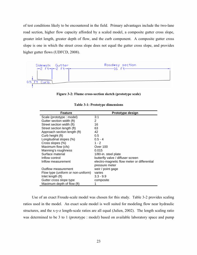
Figure 3-2: Flume cross-section sketch (prototype scale) .............................................................23
Figure 3-3: Manning’s roughness for the model-scale street section at expected flows ...............24
Figure 3-4: Curb inlet gutter panel during fabrication (Type R) ...................................................29
Figure 3-5: Combination-inlet gutter panel during fabrication (Type 13 and 16 grates) ..............29
Figure 3-6: Type 13 grate photograph ...........................................................................................30
Figure 3-7: Type 16 grate during fabrication.................................................................................30
Figure 3-8: Single No. 13 combination photograph ......................................................................31
Figure 3-9: Double No. 13 combination photograph.....................................................................31
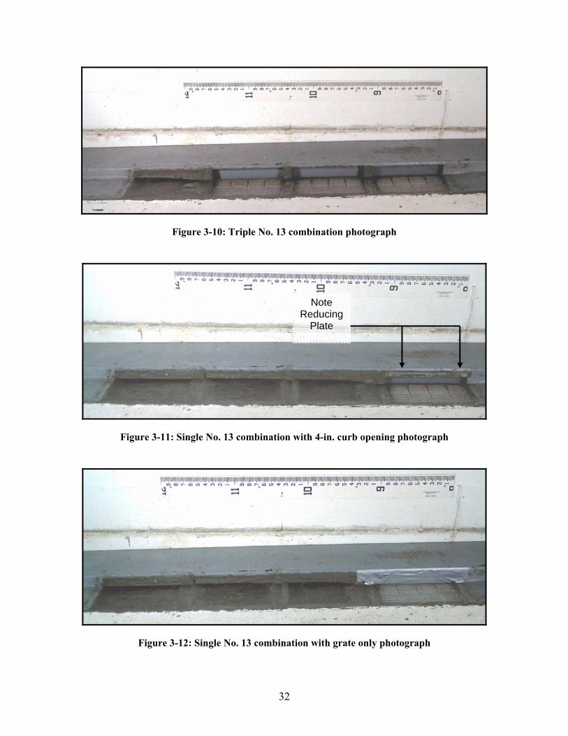
Figure 3-10: Triple No. 13 combination photograph.....................................................................32
Figure 3-11: Single No. 13 combination with 4-in. curb opening photograph..............................32
Figure 3-12: Single No. 13 combination with grate only photograph ...........................................32
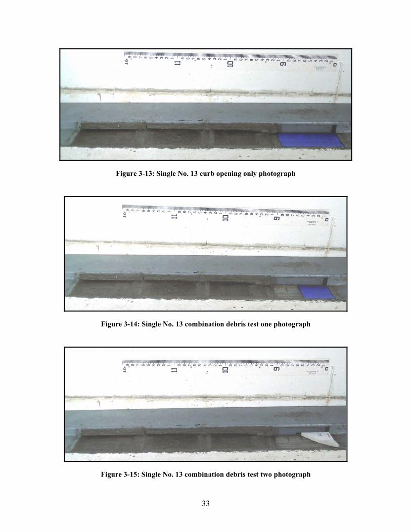
Figure 3-13: Single No. 13 curb opening only photograph ...........................................................33
Figure 3-14: Single No. 13 combination debris test one photograph ............................................33
Figure 3-15: Single No. 13 combination debris test two photograph ............................................33
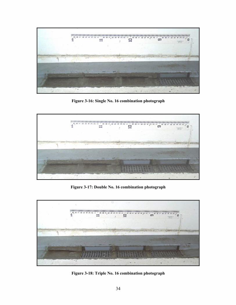
Figure 3-16: Single No. 16 combination photograph ....................................................................34
Figure 3-17: Double No. 16 combination photograph...................................................................34
Figure 3-18: Triple No. 16 combination photograph.....................................................................34
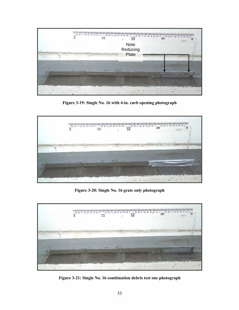
Figure 3-19: Single No. 16 with 4-in. curb opening photograph...................................................35
Figure 3-20: Single No. 16 grate only photograph ........................................................................35
iv
Figure 3-21: Single No. 16 combination debris test one photograph ............................................35
Figure 3-22: Single No. 16 combination debris test two photograph ............................................36
Figure 3-23: R5 curb inlet photograph...........................................................................................36
Figure 3-24: R9 curb inlet photograph...........................................................................................36
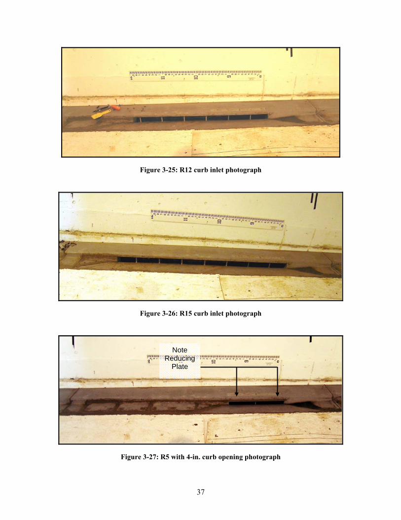
Figure 3-25: R12 curb inlet photograph.........................................................................................37
Figure 3-26: R15 curb inlet photograph.........................................................................................37
Figure 3-27: R5 with 4-in. curb opening photograph ....................................................................37
Figure 3-28: R5 with safety bar photograph ..................................................................................38
Figure 3-29: Model schematic .......................................................................................................39
Figure 3-30: Data-collection cart photograph (looking upstream) ................................................41
Figure 4-1: Type 13 combination-inlet on-grade test data.............................................................46
Figure 4-2: Type 16 combination-inlet on-grade test data.............................................................47
Figure 4-3: Type R curb inlet on-grade test data ...........................................................................47
Figure 4-4: Type 13 combination-inlet sump test data ..................................................................49
Figure 4-5: Type 16 combination-inlet sump test data ..................................................................49
Figure 4-6: Type R curb inlet sump test data.................................................................................50
Figure 5-1: Analysis flow chart .....................................................................................................52
Figure 5-2: Predicted vs. observed efficiency for Type 13 combination inlet from UDFCD methods ........................................................................................................53
Figure 5-3: Predicted vs. observed efficiency for Type 16 combination inlet from UDFCD methods ........................................................................................................54
Figure 5-4: Predicted vs. observed efficiency for Type R curb inlet from UDFCD methods.......................................................................................................................55
Figure 5-5: Predicted vs. observed efficiency for Type 13 combination inlet from improved UDFCD methods........................................................................................59
Figure 5-6: Predicted vs. observed efficiency for Type 16 combination inlet from improved UDFCD methods........................................................................................59
v
Figure 5-7: Predicted vs. observed efficiency for Type R curb inlet from improved UDFCD methods ........................................................................................................61
Figure 5-8: Predicted vs. observed efficiency for Type 13 combination-inlet from empirical equation ......................................................................................................65
Figure 5-9: Predicted vs. observed efficiency for Type 16 combination-inlet from empirical equation ......................................................................................................66
Figure 5-10: Predicted vs. observed efficiency for Type R curb inlet from empirical equation.......................................................................................................................66
Figure 5-11: Type 13 combination-inlet efficiency comparison ...................................................67
Figure 5-12: Type 16 combination-inlet efficiency comparison ...................................................67
Figure 5-13: Type R curb inlet efficiency comparison..................................................................68
Figure 5-14: Type 13 combination-inlet regression parameter sensitivity ....................................69
Figure 5-15: Type 16 combination-inlet regression parameter sensitivity ....................................69
Figure 5-16: Type R curb inlet regression parameter sensitivity...................................................70
Figure 5-17: Type 13 inlet configurations and efficiency .............................................................71
Figure 5-18: Type 16 inlet configurations and efficiency .............................................................71
Figure 5-19: Efficiency comparison from empirical equations (Type 16 inlet) ............................72
Figure 5-20: Efficiency comparison from UDFCD methods (Type 16 inlet) ...............................73
Figure 6-1: Type 13 combination-inlet efficiency from all improved methods ............................79
Figure 6-2: Type 16 combination-inlet efficiency from all improved methods ............................79
Figure 6-3: Type R curb inlet efficiency from all improved methods...........................................80
Figure A-1: Bar P-1-7/8 and Bar P-1-7/8-4 grates (UDFCD, 2008) .............................................87
Figure A-2: Bar P-1-1/8 grate (UDFCD, 2008).............................................................................88
Figure A-3: Curved vane grate (UDFCD, 2008) ...........................................................................89
Figure A-4: 45º-tilt bar grate (UDFCD, 2008) ..............................................................................90
Figure A-5: 30º-tilt bar grate (UDFCD, 2008) ..............................................................................91
Figure A-6: Reticuline grate (UDFCD, 2008) ...............................................................................92
vi
Figure D-1: Type 13 inlet specifications .....................................................................................111
Figure D-2: Type 16 inlet specifications .....................................................................................112
Figure D-3: Type R curb inlet specifications (plan view) ...........................................................113
Figure D-4: Type R curb inlet specifications (profile view)........................................................114
Figure G-1: Type 16 combination inlet .......................................................................................133
Figure G-2: Type 13 combination inlet .......................................................................................136
Figure G-3: Type R curb inlet......................................................................................................139

vii
LIST OF TABLES
Table 2-1: Summary of FHWA model characteristics ....................................................................6
Table 2-2: Composite gutter dimensions (modified from UDFCD (2008)) ....................................8
Table 2-3: Grate nomenclature and descriptions ...........................................................................11
Table 2-4: Splash-over velocity constants for inlet grates (UDFCD, 2008)..................................12
Table 3-1: Prototype dimensions ...................................................................................................23
Table 3-2: Scaling ratios for geometry, kinematics, and dynamics...............................................24
Table 3-3: Test matrix for 0.33-ft prototype flow depth................................................................26
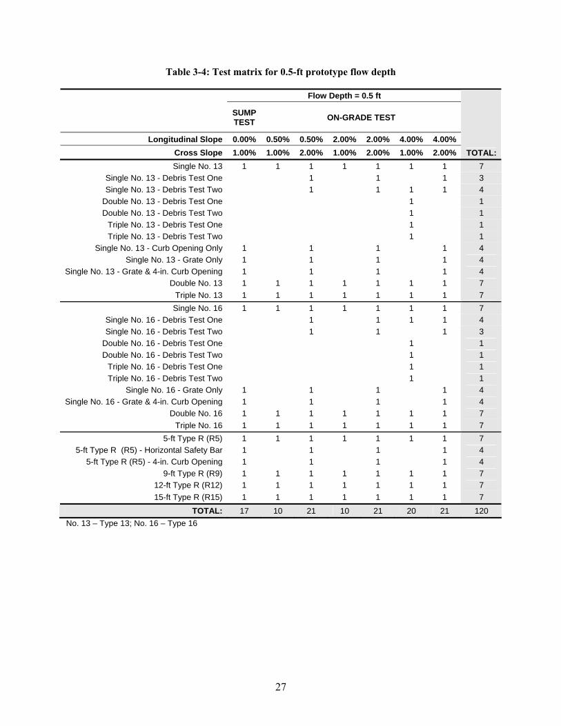
Table 3-4: Test matrix for 0.5-ft prototype flow depth..................................................................27
Table 3-5: Test matrix for 1-ft prototype flow depth.....................................................................28
Table 3-6: Additional sump tests (prototype scale) .......................................................................28
Table 3-7: Discharge measurement-instrument ranges..................................................................40
Table 3-8: Empirically-derived weir parameters ...........................................................................41
Table 4-1: Sample on-grade test data.............................................................................................46
Table 4-2: Sample sump test data ..................................................................................................48
Table 5-1: Updated splash-over velocity coefficients and plots....................................................58
Table 5-2: Empirical equations for grate and curb inlets...............................................................65
Table 5-3: Efficiency error by depth and inlet type.......................................................................75
Table B-1: 0.5% and 1% on-grade test data ..................................................................................95
Table B-2: 0.5% and 2% on-grade test data ..................................................................................96
Table B-3: 2% and 1% on-grade test data .....................................................................................98
Table B-4: 2% and 2% on-grade test data .....................................................................................99
Table B-5: 4% and 1% on-grade test data ...................................................................................101
Table B-6: 4% and 2% on-grade test data ...................................................................................102
Table B-7: Additional debris tests (4% and 1% on-grade) ..........................................................104
viii
Table C-1: Sump test data............................................................................................................107
Table C-2: Additional sump test data ..........................................................................................108
Table F-1: Additional parameters for the Type 13 inlet tests ......................................................121
Table F-2: Additional parameters for the Type 16 inlet tests ......................................................124
Table F-3: Additional parameters for the Type R curb inlet tests ...............................................127
Table H-1: Type 13 combination-inlet calculated efficiency ......................................................145
Table H-2: Type 16 combination-inlet calculated efficiency ......................................................147
Table H-3: Type R curb inlet calculated efficiency.....................................................................149

ix
LIST OF SYMBOLS, UNITS OF MEASURE, AND ABBREVIATIONS
Symbols
a gutter depression relative to the street cross slope (ft)
a width of openings between bars
a local inlet (and gutter) depression
a coefficient of discharge
a,b,c,d,e,f regression exponents
A area (ft2)
A cross-sectional flow area (ft2)
b depth exponent
b width of bars
D hydraulic depth (ft)
depth critical depth parameter
E efficiency (inlet capture) (%)
Eo ratio of flow in a depressed gutter section to total gutter flow
f function relating dimensional analysis parameters q
F, Fr Froude number
g unspecified function different from f
g acceleration due to gravity (ft/s2)
G function relating the dimensionless Pi parameters, related to the function f
h flow depth (in the gutter) (ft)
h depth for a rectangular cross section
H head above the weir crest (ft)
H total hydraulic head
L length (of grate or inlet and curb opening) (ft)
L curb opening length in the direction of flow (ft)
L2 length of the downstream slope transition
Le effective length of grate (ft)
L0 length required to trap the central portion of gutter flow
Lr length, width, and depth scaling ratio
LT curb opening length required to capture 100% of gutter flow

x
m number of dimensions required to specify the dimensions of all parameters
N Pi parameter
N coefficient of regression
n Manning roughness coefficient (or parameter)
n-1 independent parameters
nr Manning roughness scaling ratio
n-m independent dimensionless Pi parameters
Pr level of confidence that a parameter estimate has not arisen by chance
(called the significance level) evaluated by SAS
q flow bypassing the inlet
q1 dependent parameter
q2…qn n-1 independent parameters
qi parameter
Q discharge (cfs)
Q volumetric flow rate or theoretical volumetric flow rate (cfs)
Q gutter flow (cfs)
Qcaptured captured flow
Q0 total flow
Qr discharge scaling ratio
Qs flow rate in the section above the depressed section (cfs)
Qs discharge in street section (cfs) (UDFCD, 2008)
Qs total gutter flow separated into side flow
QTotal total flow
Qw flow rate in the depressed section of the gutter (cfs)
Qw captured flow
Qw total gutter flow separated into frontal flow
Qwi frontal flow intercepted by the inlet (cfs)
R hydraulic radius
Rf ratio of frontal flow captured by the inlet to the total frontal flow
Rs ratio of side flow captured to total side flow
R2 coefficient of determination for regression analysis

xi
Sc, Sc, cross slope cross (or lateral) slope
Se equivalent street cross slope (ft/ft)
Sf friction slope
SL longitudinal (street) slope (ft/ft)
So bottom slope of the channel
Sw gutter cross slope (ft/ft) (UDFCD, 2008)
Sx street cross slope (ft/ft) (UDFCD, 2008)
Sx side slope
t dividing the standard error of the parameter estimate by the estimate itself
in SAS
T top width of gutter flow
T top width for a general cross section
T top width of flow (spread) (ft) (UDFCD, 2008)
T top width of flow spread from the curb face (ft)
Ts spread of flow in street (ft) (UDFCD, 2008)
Tw top width parameter
V velocity (of cross-sectional averaged flow, flow in the gutter, and
approaching flow) (ft/s)
V velocity of flow at the inlet (ft/s), determined from Q/A
V cross-sectional average flow velocity (ft/s)
Vo splash-over velocity (ft/s)
V0 velocity of approaching flow
Vr velocity scaling ratio
velocity flow velocity parameter
W width (of the gutter, gutter section, and depressed gutter section) (ft)
W width of gutter pan (ft) (UDFCD, 2008)
Wp wetted perimeter
y depth (of flow in the gutter and flow in the depressed gutter section) (ft)
y0 depth of flow over the first opening
α,β,γ,η constants (UDFCD, 2008)
θ angle formed by the curb and gutter

xii
Π Pi parameter for dimensional analysis
Φ unit conversion constant, equal to 1.49 for U. S. Customary and 1.00 for
SI
Units of Measure
acre ft acre foot
cfs cubic feet per second
º degree(s), as a measure of angular distance
ft feet or foot
ft/ft feet per foot
ft/s feet per second
ft/s2 feet per second squared
ft2 square feet
GB gigabyte(s)
hp horse power
in. inch(es)
% percent
SI International System of Units
Abbreviations
3d type 2 debris
annubar differential pressure meter
AT additional test
BMP Best Management Practice
CDOT Colorado Department of Transportation
CSU Colorado State University
DP differential pressure
ERC Engineering Research Center
FHWA Federal Highway Administration
flat type 1 debris
HEC 22 Hydraulic Engineering Circular 22

xiii
ID identification
mag meter electro-magnetic flow meter
No. number
QC quality control ® registered
R5 5-ft Type R curb inlet
R9 9-ft Type R curb inlet
R12 12-ft Type R curb inlet
R15 15-ft Type R curb inlet
SAS Statistical Analysis Software
SDHC Secure Digital High Capacity TM trademark
Type 13, Type 16 UDFCD grates tested at CSU
Type R CDOT curb tested at CSU
UDFCD Urban Drainage and Flood Control District
USB Universal Serial Bus
USBR U. S. Bureau of Reclamation
USDCM Urban Storm Drainage Criteria Manual

xiv
1
1 INTRODUCTION
A research program was conducted at Colorado State University (CSU) to evaluate the
hydraulic efficiency of three storm-drain inlets. Inlets tested in this study are currently used by
the Urban Drainage and Flood Control District (UDFCD) of Denver, and consist of the Denver
Type 13 and 16 grates, and the Colorado Department of Transportation (CDOT) Type R curb.
These inlets have never been specifically studied or tested for development of hydraulic
efficiency relationships. Current design practices are based upon a document produced by the
Federal Highway Administration (FHWA, 2001) titled “Hydraulic Engineering Circular 22”
(HEC 22). General inlet types are addressed in HEC 22, but no specific guidance is provided
for these three inlets used by the UDFCD. The study presented in this report focused on
collecting data on these inlets under physically-relevant design conditions, and developing
improved design methods for determining inlet efficiency under varying road geometries. A 1/3
Froude-scale model of a two-lane road section was designed and built at the Engineering
Research Center (ERC) of CSU. The model consisted of an adjustable slope road surface, gutter
panels, and three interchangeable inlet types positioned in a testing flume. Details pertaining to
model construction, testing procedure, resulting database, and data analysis are presented in this
report.
1.1 Project Background Storm-water runoff is typically conveyed through a network comprised of streets, gutters,
inlets, storm sewer pipes, and treatment facilities. Streets of developed areas often serve as
collectors for runoff, and convey water into gutters and eventually to storm sewer inlets. Storm-
water management in the metropolitan Denver area falls under the jurisdiction of the UDFCD.
Policies, design procedures, and Best Management Practices (BMPs) are provided in the “Urban
Storm Drainage Criteria Manual” (USDCM; UDFCD, 2008). Design methods presented in the

2
USDCM for determining inlet efficiency provide the currently accepted methodology for design
of storm-water collection systems throughout the region depicted in Figure 1-1. Guidance is
provided in the USDCM for local jurisdictions, developers, contractors, and industrial and
commercial operations in selecting, designing, maintaining, and carrying-out BMPs to
effectively handle storm-water runoff (UDFCD, 2008). Other agencies participating in this study
include the University of Colorado at Denver and the Colorado Department of Transportation.
Figure 1-1: Map of the Urban Drainage and Flood Control District (UDFCD, 2008)
The need for this study arose from uncertainty in selecting appropriate design equations
presented in the USDCM for the Type 13, 16, and R inlets. Local jurisdictions depicted in Figure

3
1-1 often require use of these three inlets. Methods presented in the USDCM for determining
efficiency of grate and curb inlets were adopted from HEC 22, and do not include these three
inlets. When the most similar inlets in the USDCM were selected for calculation purposes,
uncertainties in sizing the inlets and in the level of flood protection afforded by them were
realized. Uncertainty in design practice often leads to over-design and wasted expense. A need
existed for greater accuracy in design for the three inlets tested in this study. Results of this
research program will be used to supplement the USDCM design methodology.
Improving the accuracy of current design methods for the three inlets tested in this study
requires addressing several deficiencies that exist in the procedures given in the USDCM (from
HEC 22). Seven grate inlets are specified in HEC 22 and some are similar to, but not exactly the
same as, the Type 13 and 16 grates tested in this study. Subtle differences exist in the flow area
and geometry of the grates. A second difference relates to the use of what is commonly referred
to as a “combination inlet,” a term used when a grate and a curb inlet are used together.
Guidance provided in the USDCM is to ignore the curb inlet and determine efficiency based
solely on the grate capacity. Some degree of conservatism is provided when determining
efficiency in this manner, but performance of the combination inlet may be under-predicted
when flow submerges the grate portion. A third difference relates to the curb inlet design used.
The curb inlet specified in HEC 22 is of a general type, with design parameters that do not fully
describe the Type R curb inlet used by the UDFCD. Differences exist in the dimensions of the
local inlet depression for the Type R curb inlet that are not considered in the HEC 22
calculations. The Type R curb inlet depression is greater than what is described in HEC 22 and
capable of capturing some degree of additional flow. Lastly, typical design practices in the
USDCM are based on the assumption of steady, uniform gutter flow. Hydraulics of street flow
may or may not be uniform in any given situation, and the assumption of uniform flow may not
be entirely valid. The relevance of uniform flow in analysis of the test data will be examined.
1.2 Research Objectives A testing program was developed by the UDFCD to address known deficiencies in the
USDCM design methods, and the primary purpose of this study was to collect data for further
analysis by the UDFCD. After testing was completed, an analysis was performed to illustrate
how current design methods given in the USDCM can be improved.

4
Objectives of this project were to:
• Construct a 1/3 scale model of a two-lane roadway with adjustable street slopes,
gutter panels, and interchangeable inlet types.
• Collect data on total, captured, and bypassed flow for each inlet type, flow depth, and
slope configuration.
• Determine efficiency for each test configuration as the ratio of captured flow to total
input flow.
• Provide qualitative and quantitative interpretation of the performance of each
configuration tested.
• Provide relevant analysis of the data to improve current design methods given in the
USDCM for the inlets tested.
1.3 Report Organization This report presents the project background and research objectives, literature review,
description of the test facility and model fabrication, test data, analysis and results, and
conclusions and recommendations. Included in each of the reports is a CD that contains the
report Microsoft Word® (.doc) and Adobe® Acrobat® (.pdf) files, along with the Microsoft
Excel® (.xls) analysis spreadsheet files. Also provided with this report is an Electronic Data
Supplement (stored on a 16-GB SDHCTM card) that contains the CD contents and all test data
and photographic documentation. Because only one SDHCTM card is provided and will not
accompany each report, the reader is referred to the UDFCD for obtaining photographs and
video documentation.
5
2 LITERATURE REVIEW
Urban storm drainage is an extensive topic that can range in scope from application of
BMPs at a system level, to analysis of any given component in a large drainage network. Inlets
tested in this study are used at the component level. The scope of this literature review is to
provide background necessary for use of the collected test data in developing improved design
methods. This chapter describes the model utilized to supply data for development of current
UDFCD design methods for grate and curb inlets. Current design methods are explained and
equations are presented from the USDCM. Two velocity-depth numerical relationships
commonly known as Manning’s equation and the Froude number are defined. The dimensional
analysis method, which is commonly used for developing equations to predict observed test data,
is explained.
2.1 Relevant Street Drainage Studies HEC 22 was developed, in part, from a FHWA report titled “Bicycle-safe Grate Inlets
Study.” Ultimately, it was that FHWA study that provided data for development of the inlet
equations provided in HEC 22 and used in the USDCM for the Type 13 and 16 inlets. Volume 1
of the FHWA study titled “Hydraulic and Safety Characteristics of Selected Grate Inlets on
Continuous Grades” (FHWA, 1977) describes the model built and the testing methods used.
Table 2-1 provides a summary of physical characteristics of the FHWA model.

6
Table 2-1: Summary of FHWA model characteristics
Feature FHWA Scale (prototype : model) 1:1 Gutter section width (ft) 2 Street section width (ft) 6 Street section length (ft) 60 Approach section length (ft) none Curb height (ft) none Longitudinal slopes (%) 0.5 - 13 Cross slopes (%) 2 - 6.25 Maximum flow (cubic feet per second (cfs)) 5.6 Manning’s roughness 0.016 - 0.017 Surface material 3/4-in. PermaPly® (fiberglass) Inflow control vertical sluice gate Inflow measurement Orifice-Venturi meter Outflow measurement weir / J-hook gage Flow type (uniform or non-uniform) uniform Inlet length (ft) 2 - 4 Gutter cross slope type uniform Maximum depth of flow (ft) 0.45
A total of eleven grate inlets were tested for structural integrity and bicycle-safety
characteristics in the FHWA study. Of these, seven were tested hydraulically under the
conditions given previously in Table 2-1. Efforts were made to separately measure frontal-
captured flow and side-captured flow by blocking-off portions of the inlet opening. Grate
efficiency was defined as the ratio of captured flow to total street flow. Flow into the model was
from a large headbox reservoir. The vertical sluice gate was used to provide flow control from
the headbox at the upstream end of the road section, and to ensure uniform flow conditions in the
model. A total of 1,680 tests were carried out at the U. S. Bureau of Reclamation (USBR)
Hydraulic Laboratory. Several of the qualitative findings are summarized here:
• Grates with wide longitudinal bar spacing were found to perform the best.
• For a given width of flow spread, grates were most efficient at flatter slopes.
• For a constant gutter flow and cross slope, grate efficiency increased as longitudinal
slope was increased.
• Longer grates reached higher efficiencies at steeper slopes than shorter grates.
• Velocity is the factor that determined the most efficient longitudinal slope.
• At test conditions where splash carried completely across one or more of the grate
designs, differences in efficiency were caused mostly by the grate type.
7
• All grates showed patterns of increasing efficiency with increased flow and
longitudinal slope until the increased velocity caused splashing completely across the
grate.
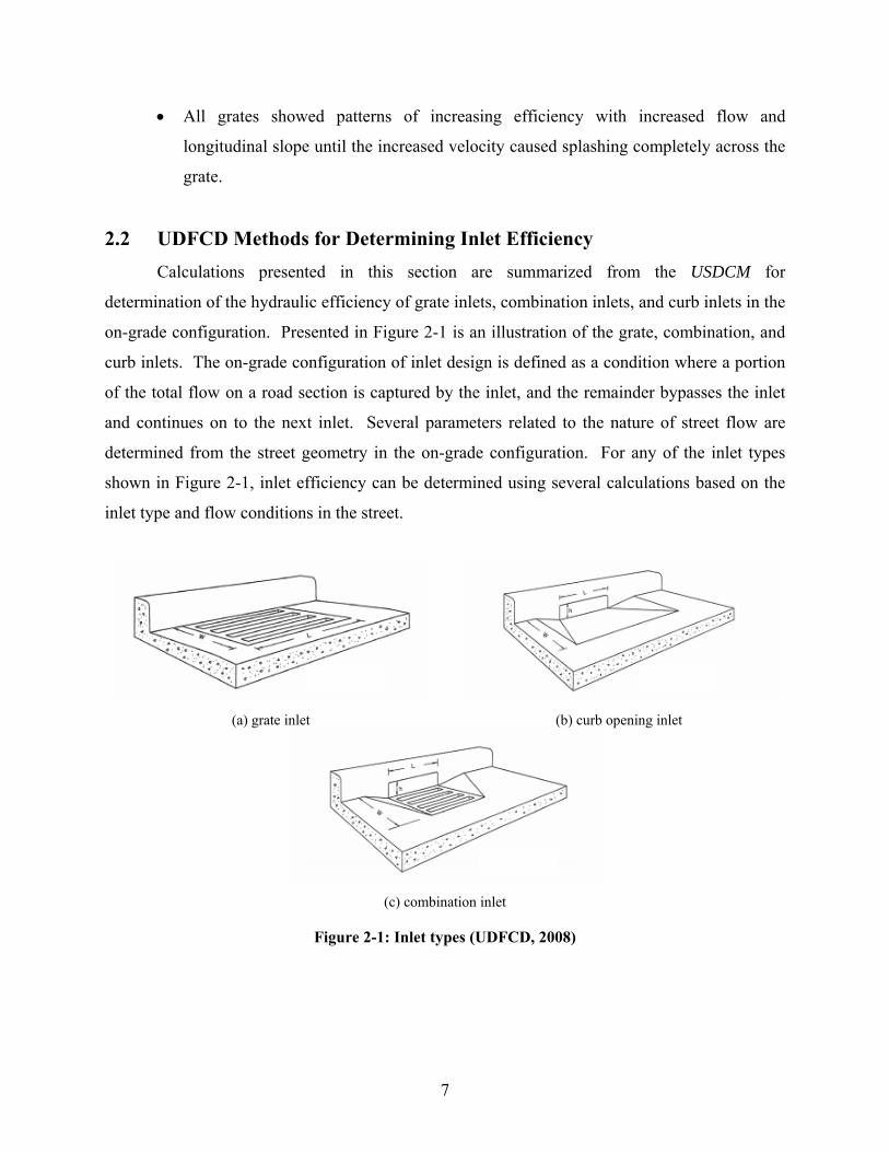
2.2 UDFCD Methods for Determining Inlet Efficiency Calculations presented in this section are summarized from the USDCM for
determination of the hydraulic efficiency of grate inlets, combination inlets, and curb inlets in the
on-grade configuration. Presented in Figure 2-1 is an illustration of the grate, combination, and
curb inlets. The on-grade configuration of inlet design is defined as a condition where a portion
of the total flow on a road section is captured by the inlet, and the remainder bypasses the inlet
and continues on to the next inlet. Several parameters related to the nature of street flow are
determined from the street geometry in the on-grade configuration. For any of the inlet types
shown in Figure 2-1, inlet efficiency can be determined using several calculations based on the
inlet type and flow conditions in the street.
(a) grate inlet (b) curb opening inlet
(c) combination inlet
Figure 2-1: Inlet types (UDFCD, 2008)
8
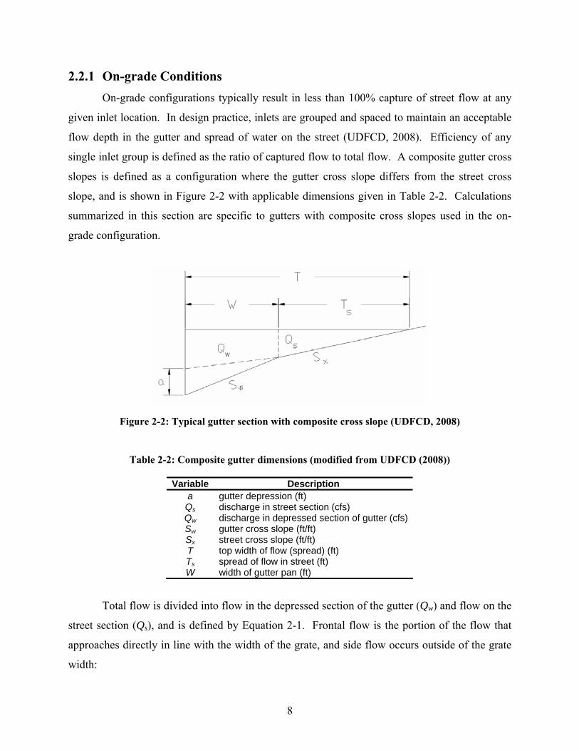
2.2.1 On-grade Conditions On-grade configurations typically result in less than 100% capture of street flow at any
given inlet location. In design practice, inlets are grouped and spaced to maintain an acceptable
flow depth in the gutter and spread of water on the street (UDFCD, 2008). Efficiency of any
single inlet group is defined as the ratio of captured flow to total flow. A composite gutter cross
slopes is defined as a configuration where the gutter cross slope differs from the street cross
slope, and is shown in Figure 2-2 with applicable dimensions given in Table 2-2. Calculations
summarized in this section are specific to gutters with composite cross slopes used in the on-
grade configuration.
Figure 2-2: Typical gutter section with composite cross slope (UDFCD, 2008)
Table 2-2: Composite gutter dimensions (modified from UDFCD (2008))
Variable Description a gutter depression (ft) Qs discharge in street section (cfs) Qw discharge in depressed section of gutter (cfs) Sw gutter cross slope (ft/ft) Sx street cross slope (ft/ft) T top width of flow (spread) (ft) Ts spread of flow in street (ft) W width of gutter pan (ft)
Total flow is divided into flow in the depressed section of the gutter (Qw) and flow on the
street section (Qs), and is defined by Equation 2-1. Frontal flow is the portion of the flow that
approaches directly in line with the width of the grate, and side flow occurs outside of the grate
width:

9
sw QQQ += Equation 2-1
where:
Q = volumetric flow rate (cfs); Qw = flow rate in the depressed section of the gutter (cfs); and Qs = flow rate in the section above the depressed section (cfs).
Theoretical total flow rate in a composite gutter section can be computed using Equation
2-2:
o
s
EQ
Q−
=1
Equation 2-2
where:
Q = theoretical volumetric flow rate (cfs); Qs = flow rate in the section above the depressed section (cfs); and Eo = ratio of flow in the depressed section of the gutter to the total gutter flow (and is defined
below).
The ratio of flow in the depressed section of the gutter to the total gutter flow (Eo) can be
found from Equation 2-3:
( ) 11
1
1
1
38
−⎥⎦
⎤⎢⎣
⎡−
+
+=
WTSS
SSE
xw
xwo Equation 2-3
where:
Sw = gutter cross slope (ft/ft) (and is defined below); Sx = street cross slope (ft/ft); W = width of the gutter section (ft); and T = total width of flow (ft).
Gutter cross slope is defined from Equation 2-4:
WaSS xw += Equation 2-4

10
where:
Sw = gutter cross slope (ft/ft); Sx = street cross slope (ft/ft); a = gutter depression relative to the street cross slope (ft); and W = width of the gutter (ft).
Equation 2-5 and Equation 2-6 can be derived from the gutter geometry presented
previously in Figure 2-2:
xTSay += Equation 2-5
and
aWTSA x 21
21 2 += Equation 2-6
where:
A = cross-sectional flow area (ft2); T = total width of flow (ft); Sx = street cross slope (ft/ft); W = width of the gutter (ft); a = gutter depression relative to the street cross slope (ft); and y = depth of flow in the depressed gutter section (ft).
From Equation 2-1 through 2-6, gutter flow, street flow, and the depth and spread of flow
on the street can be determined. With these quantities known, inlet efficiency can be determined
for grate and curb inlets as described in the following sections.
2.2.2 Grate Inlets Grate inlet efficiency is governed by the grate length and width, and is reduced when
width of flow is greater than the grate width, or the flow has sufficient velocity to splash over the
inlet. Table 2-3 describes the grates given in the USDCM and corresponding schematics are
provided in Appendix A. Determination of grate inlet efficiency as presented in the USDCM
requires that total gutter flow be separated into frontal flow (Qw) and side flow (Qs), which were
defined previously. Side flow can be found from Equation 2-2 and from Equation 2-1 the frontal
flow can be determined.
11
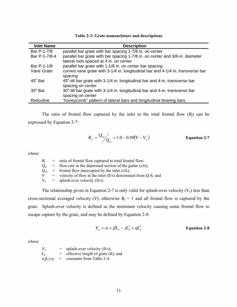
Table 2-3: Grate nomenclature and descriptions
Inlet Name Description Bar P-1-7/8 parallel bar grate with bar spacing 1-7/8 in. on center Bar P-1-7/8-4 parallel bar grate with bar spacing 1-7/8 in. on center and 3/8-in. diameter
lateral rods spaced at 4 in. on center Bar P-1-1/8 parallel bar grate with 1-1/8 in. on center bar spacing Vane Grate curved vane grate with 3-1/4 in. longitudinal bar and 4-1/4 in. transverse bar
spacing 45o Bar 45o-tilt bar grate with 3-1/4 in. longitudinal bar and 4-in. transverse bar
spacing on center 30o Bar 30o-tilt bar grate with 3-1/4 in. longitudinal bar and 4-in. transverse bar
spacing on center Reticuline “honeycomb” pattern of lateral bars and longitudinal bearing bars
The ratio of frontal flow captured by the inlet to the total frontal flow (Rf) can be
expressed by Equation 2-7:
( )ow
wif VVQ
QR −−== 09.00.1 Equation 2-7
where:
Rf = ratio of frontal flow captured to total frontal flow; Qw = flow rate in the depressed section of the gutter (cfs); Qwi = frontal flow intercepted by the inlet (cfs); V = velocity of flow at the inlet (ft/s) determined from Q/A; and Vo = splash-over velocity (ft/s).
The relationship given in Equation 2-7 is only valid for splash-over velocity (Vo) less than
cross-sectional averaged velocity (V), otherwise Rf = 1 and all frontal flow is captured by the
grate. Splash-over velocity is defined as the minimum velocity causing some frontal flow to
escape capture by the grate, and may be defined by Equation 2-8:
32eeeo LLLV ηγβα +−+= Equation 2-8
where:
Vo = splash-over velocity (ft/s); Le = effective length of grate (ft); and α,β,γ,η = constants from Table 2-4.

12
Constants in Equation 2-8 are associated with specific grates listed in Table 2-4.
Table 2-4: Splash-over velocity constants for inlet grates (UDFCD, 2008)
Type of Grate α β γ η Bar P-1-7/8 2.22 4.03 0.65 0.06 Bar P-1-1/8 1.76 3.12 0.45 0.03 Vane Grate 0.30 4.85 1.31 0.15 45º Bar 0.99 2.64 0.36 0.03 Bar P-1-7/8-4 0.74 2.44 0.27 0.02 30º Bar 0.51 2.34 0.20 0.01 Reticuline 0.28 2.28 0.18 0.01
The ratio of side flow captured to total side flow approaching the grate can be determined
using Equation 2-9:
3.2
8.115.01
1
LSV
R
x
s
+= Equation 2-9
where:
Rs = ratio of side flow captured to total side flow; Sx = side slope; L = length of grate (ft); and V = velocity of flow in the gutter (ft/s).
Capture efficiency of a grate inlet may be determined using Equation 2-10, which uses
the parameters determined previously:
⎟⎟⎠
⎞⎜⎜⎝
⎛+⎟⎟
⎠
⎞⎜⎜⎝
⎛=
RQ
QRE s
sw
f Equation 2-10
where:
E = grate inlet efficiency; Rs = ratio of side flow captured to total side flow; Rf = ratio of frontal flow captured to total frontal flow; Q = volumetric flow rate (cfs); Qw = flow rate in the depressed section of the gutter (cfs); and Qs = flow rate in the section above the depressed section (cfs).
Efficiency for combination inlets is typically determined by only considering the grate
when the curb opening and grate are of equal length (UDFCD, 2008), and Equation 2-10 is used.
13
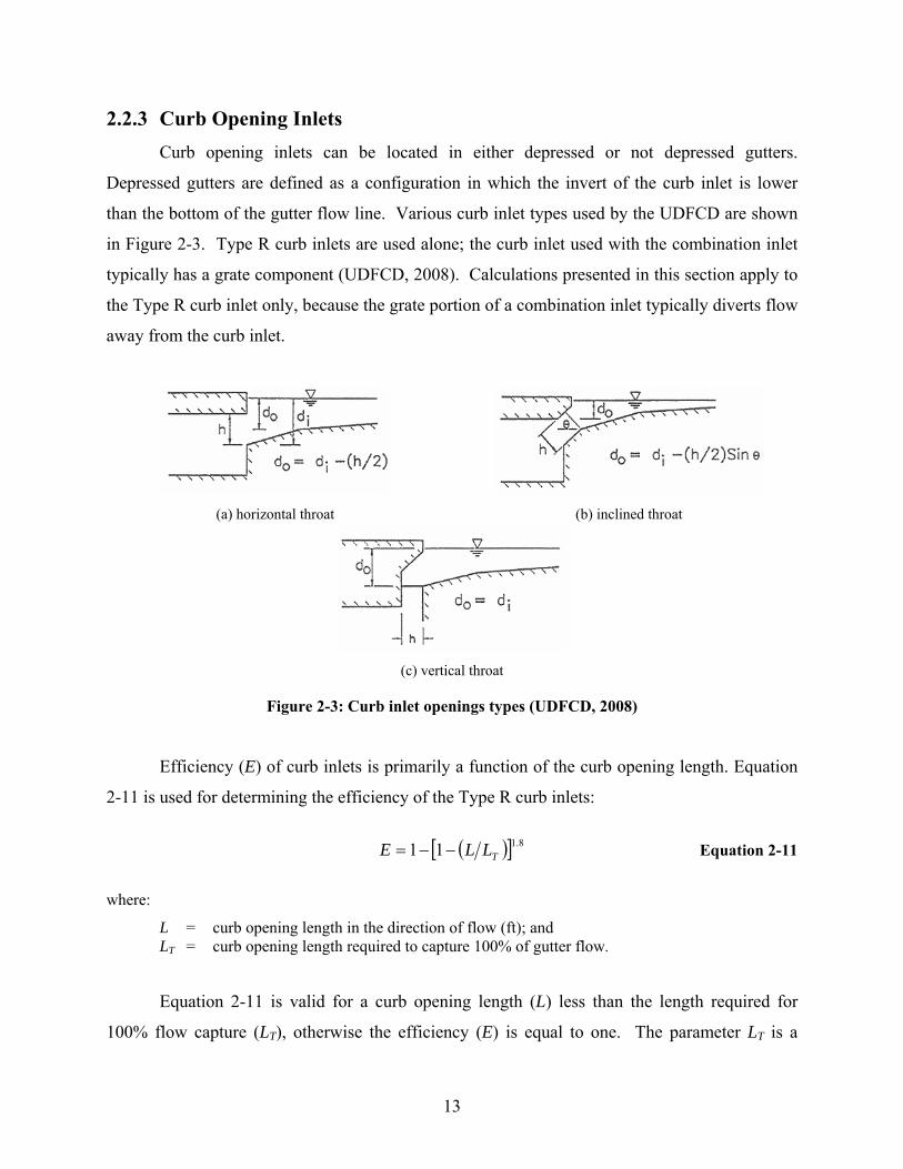
2.2.3 Curb Opening Inlets Curb opening inlets can be located in either depressed or not depressed gutters.
Depressed gutters are defined as a configuration in which the invert of the curb inlet is lower
than the bottom of the gutter flow line. Various curb inlet types used by the UDFCD are shown
in Figure 2-3. Type R curb inlets are used alone; the curb inlet used with the combination inlet
typically has a grate component (UDFCD, 2008). Calculations presented in this section apply to
the Type R curb inlet only, because the grate portion of a combination inlet typically diverts flow
away from the curb inlet.
(a) horizontal throat (b) inclined throat
(c) vertical throat
Figure 2-3: Curb inlet openings types (UDFCD, 2008)
Efficiency (E) of curb inlets is primarily a function of the curb opening length. Equation
2-11 is used for determining the efficiency of the Type R curb inlets:
( )[ ] 8.111 TLLE −−= Equation 2-11
where:
L = curb opening length in the direction of flow (ft); and LT = curb opening length required to capture 100% of gutter flow.
Equation 2-11 is valid for a curb opening length (L) less than the length required for
100% flow capture (LT), otherwise the efficiency (E) is equal to one. The parameter LT is a

14
function of street characteristics and the storm-water discharge in the street. For an inlet located
in a gutter that is not depressed relative to the street slope, Equation 2-12 applies:
6.0
3.042.0 16.0 ⎟⎟⎠
⎞⎜⎜⎝
⎛=
xLT nS
SQL Equation 2-12
where:
Q = gutter flow (cfs); SL = longitudinal street slope (ft/ft); Sx = street cross slope (ft/ft); and n = Manning’s roughness coefficient.
For an inlet that is depressed relative to the street slope, Equation 2-13 applies:
6.0
3.042.0 16.0 ⎟⎟⎠
⎞⎜⎜⎝
⎛=
eLT nS
SQL Equation 2-13
where:
LT = curb opening length required to capture 100% of gutter flow; Q = gutter flow (cfs); SL = longitudinal street slope (ft/ft); Se = equivalent street cross slope (ft/ft); and n = Manning’s roughness coefficient.
The equivalent street cross slope (Se) required for Equation 2-13 is determined from
Equation 2-14:
oxe EWaSS += Equation 2-14
where:
Sx = street cross slope (ft/ft); a = gutter depression (ft); W = depressed gutter section width (ft), illustrated in Figure 2-2; and Eo can be found using Equation 2-3.
Once the parameter LT has been determined, efficiency of the curb inlet may be
calculated using Equation 2-11.

15
2.3 Manning’s Equation Uniform flow is a state of open-channel flow that occurs when accelerating and
decelerating forces acting on the flow are equal (Chaudhry, 2008). In this state, the channel
itself exerts hydraulic control over the flow. Often, uniform flow occurs in long and straight
prismatic channels that do not vary in bottom slope or cross-sectional character with distance.
Flow depth corresponding to uniform flow is called normal depth. The numerical relationship of
Manning’s equation commonly used to describe uniform flow is provided as Equation 2-15.
Known channel geometry, flow depth, roughness, and bottom slope can be used in Manning’s
equation to solve for flow velocity. Alternatively, surface roughness can be solved for. The
friction slope (Sf) term in Manning’s equation represents the rate of energy dissipation caused by
frictional forces acting along the channel perimeter. When a state of uniform flow exists, the
friction slope is equal to the bottom slope of the channel (So). Manning’s equation is then
simplified by assuming that Sf is equal to So. Conversely, Manning’s equation can provide an
explicit solution for the friction slope when uniform flow does not exist:
2 1
3 2fV R S
nΦ
= Equation 2-15
where:
V = cross-sectional averaged flow velocity (ft/s); Φ = unit conversion constant, equal to 1.49 for U. S. Customary and 1.00 for SI; R = hydraulic radius (ft), which is a function on depth; Sf = friction slope; and n = Manning’s roughness coefficient. 2.4 Froude Number
In open-channel flow, where gravity is the driving force, the Froude number represents
the ratio of inertial to gravity forces (Chaudhry, 2008). Stated another way, it is the ratio of bulk
flow velocity to elementary gravity wave celerity. The Froude number (Fr) is defined as
Equation 2-16:
gDVFr = Equation 2-16

16
where:
V = cross-sectional average flow velocity (ft/s); g = acceleration due to gravity (ft/s2); and D = hydraulic depth (ft), equal to area (A) divided by top width (T) for a general cross section
or depth (h) for a rectangular cross section.
The celerity of an elementary gravity wave is defined as the velocity with which the wave
travels relative to the bulk flow velocity (Chaudhry, 2008). When the Froude number is greater
than one, for flow velocity greater than wave celerity, a disturbance in the flow can only
propagate in the direction of flow. This type of flow is commonly classified as supercritical.
When the Froude number is less than one, for flow velocity less than wave celerity, a disturbance
in the flow can propagate either upstream of downstream. This type of flow is commonly
classified as subcritical.
2.5 Dimensional Analysis Development of equations by the process of dimensional analysis requires identifying
and utilizing parameters that are significant in describing the process or phenomena in question.
A survey of parameter groups identified as significant in determining inlet efficiency is presented
in this section. Many phenomena in fluid mechanics depend, in a complex way, on geometric
and flow parameters (Fox, 2006). For open-channel street flow, such parameters are associated
with the geometry of the street and gutter sections, and the flow velocity. Through the process of
dimensional analysis, significant parameters are combined to produce dimensionless quantities
that are descriptive of the phenomena in question. One approach to developing equations is to
collect experimental data on these dimensionless quantities and fit a mathematical model to
them.
The Buckingham Pi theorem is a method for determining dimensionless groups that
consist of parameters identified as significant. The theorem is a statement of the relation between
a function expressed in terms of dimensional parameters and a related function expressed in
terms of non-dimensional parameters (Fox, 2006). Given a physical problem in which the
dependent parameter is a function of n-1 independent parameters, the relationship among the
variables can be expressed in functional form as Equation 2-17:
)...,,,( 321 nqqqfq = or 0)...,,,( 21 =nqqqg Equation 2-17

17
where:
q1 = dependent parameter; q2…qn = n-1 independent parameters; f = function relating dimensional analysis parameters q; and g = unspecified function different from f.
The Buckingham Pi theorem states that, given a relation among n parameters in the form
of Equation 2-17, the n parameters may be grouped into n-m independent dimensionless ratios
also called Pi (Π) groups (Fox, 2006). In functional form this is expressed as Equation 2-18:
)...,,,( 3211 mnG −ΠΠΠ=Π or 0)...,,,( 21 =ΠΠΠ −mnG Equation 2-18
where:
Π = Pi parameter; and G = function relating the dimensionless Pi parameters, related to the function f.
The number m is often, but not always, equal to the number of dimensions required to
specify the dimensions of all the parameters (qi) of the problem or phenomena in question. The
n-m dimensionless Pi parameters obtained from this procedure are independent of one another.
The Buckingham Pi theorem does not predict the functional form of G, which must be
determined experimentally.
2.6 Significant Parameter Groups for Calculating Inlet Efficiency A review of available literature has shown that the complex nature of street inlet flow has
precluded the development of purely theoretical equations. Often the approach of developing
empirical equations has been used. Physical variables related to gutter flow and inlet
characteristics are typically identified and combined into meaningful parameter groups using
dimensional analysis. Tests are performed on parameter groups to quantify their relevance.
Although the method of dimensional analysis is universally applicable to development of
parameter groups, there are many forms that these dimensionless groups may take depending
upon what parameters are used. Two of the larger studies conducted on the topic of inlet
efficiency were the FHWA study on bicycle-safe grate inlets described previously (FHWA,
1977) and a study completed at The Johns Hopkins University (Li, 1956). Equations developed
from the FHWA study were incorporated into HEC 22 and were presented previously. The
Johns Hopkins University study took a slightly different approach of regression analysis. For an

18
un-depressed grate inlet with longitudinal bars, the following parameter groups in Equation 2-19
were identified:
⎟⎟⎠
⎞⎜⎜⎝
⎛=
ay
ba
gyV
fyg
VL 0
0
0
00
0 ,, Equation 2-19
where:
L0 = length required to trap the central portion of gutter flow; V0 = velocity of approaching flow; y0 = depth of flow over the first opening; g = unspecified function different from f; a = width of openings between bars; and
b = width of bars.
For a depressed curb inlet, the following parameter groups in Equation 2-20 were
identified:
⎟⎟⎠
⎞⎜⎜⎝
⎛=
0
22
aL
aL
gyVf
gyLyQ θ Equation 2-20
where:
Q = captured flow; Q0 = total flow; θ = angle formed by the curb and gutter; L = length of the curb opening; L2 = length of the downstream slope transition; V = velocity of approaching flow; y = depth of flow in the gutter; g = acceleration due to gravity; a = local inlet depression; and q = flow bypassing the inlet.
For both of these inlets, the Froude number appears as a parameter group, as do several
length and flow ratios.
In a study performed at the Istanbul Technical University (Uyumaz, 2002), several
parameter groups were identified in Equation 2-21 for a depressed curb opening inlet in a gutter
with uniform cross section (for a uniform gutter cross section, the gutter slope is equal to the
street cross slope):

19
⎟⎟⎠
⎞⎜⎜⎝
⎛=
hL
FTLfQ w
w ,, Equation 2-21
where:
Q = total flow; Qw = captured flow; L = inlet length; F = Froude number; T = top width of gutter flow; and h = depth of flow in the gutter.
For this inlet, the Froude number appears in the first parameter group, and ratios of
lengths and flows are used. The flow ratio used is typically called the inlet efficiency or capture
efficiency.
2.7 Summary Currently-accepted design procedures, which represent the state-of-the-art for inlet design
from the UDFCD, were explained for each inlet used in this study. USDCM methods (which
originated in HEC 22) are based upon theoretical parameters which must be determined from
empirical relationships. The FHWA model, which provided data for development of HEC 22
methods, was described. In addition, Manning’s equation and the Froude number were each
defined as unique velocity-depth relationships. The process of dimensional analysis was
explained as a commonly-used method for developing significant parameter groups that can be
used in equation development. A survey of parameter groups identified as significant in
determining inlet efficiency was conducted. Empirical equations have been used for determining
the capacity of curb and grate inlets for composite gutter sections (in which the gutter cross slope
does not equal the street cross slope). Most of the available research has been on gutters with
uniform cross slopes. For gutters of uniform cross slope, Manning’s equation for a triangular
cross section is frequently used for determining flow. Relationships exist for determining either
curb or grate inlet capacity. Few relationships exist for combination inlets; they are typically
treated as only a grate inlet. This is due to the observation that, when the grate is not depressed
below the gutter flow line, little or no gain in performance results from the grate. A need exists
for design equations, based on physically relevant and easy to determine parameters, which
address use of combination inlets with the grate depressed below the gutter flow line.

20

21
3 HYDRAULIC MODELING
Testing was performed on three different types of curb and grate inlet from January 2006
through November 2008. Emphasis was placed on collection of curb depth and flow data to
facilitate completion of research objectives. Two basic street drainage conditions were tested in
this study for a total of 318 tests. First was a sump condition, in which all of the street flow was
captured by the inlets. Second was an on-grade condition, in which only a portion of the total
street flow was captured and the rest of the flow bypassed the inlets. All three inlets (Type 13,
Type 16, and Type R) were tested in the sump and on-grade conditions at three depths. With
development of the model and testing program for this study, there was an opportunity to
improve upon the FHWA model. This chapter provides details of the testing facility, conditions
tested, model construction, and testing methods used in obtaining data.
3.1 Testing Facility Description and Model Scaling Model construction and testing was performed at the ERC of Colorado State University.
A photograph of the flume, pipe network, and drainage facilities is presented in Figure 3-1. The
model consisted of a headbox to supply water, a flume section containing the street and inlets,
supporting pumps, piping, several flow-measurement devices, a tailbox to capture returning
flow, and the supporting superstructure.

22
Figure 3-1: Photograph of model layout
Contained within the flume section were the model’s road surface and all curb and inlet
components. Sufficient laboratory space allowed for construction of a two-lane street surface. A
cross section of the flume including the street section, gutter panel, and sidewalk is presented in
Figure 3-2. The street section was constructed as a 2-by-4 in. tubular steel framework and
decked with 1/8-in. thick sheet steel. Slope adjustment was achieved by the use of eight scissor
jacks placed under the street section, and adjustment ranged from 0.5% to 4% longitudinally and
from 1% to 2% laterally. Upstream of the street section, an approach section was constructed to
allow flow to stabilize after exiting the headbox. A diffuser screen was installed at the junction
between the headbox and the approach section to minimize turbulence and to distribute flow
evenly across the width of the model. The long horizontal approach section provided stabilized
flow. Prototype dimensions and characteristics are presented in Table 3-1, which can be directly
compared to Table 2-1 for the FHWA model. The physical model used provided a broader range
Headbox
Sharp-crested Weirs
Pumps
Pipe Network
Tailbox
Inlets
Sump Inlet
Street Section
Flume Section
23
of test conditions likely to be encountered in the field. Primary advantages include the two-lane
road section, higher flow capacity afforded by a scaled model, a composite gutter cross slope,
greater inlet length, greater depth of flow, and the curb component. A composite gutter cross
slope is one in which the street cross slope does not equal the gutter cross slope, and provides
higher gutter flows (UDFCD, 2008).
Figure 3-2: Flume cross-section sketch (prototype scale)
Table 3-1: Prototype dimensions
Feature Prototype design Scale (prototype : model) 3:1 Gutter section width (ft) 2 Street section width (ft) 16 Street section length (ft) 63 Approach section length (ft) 42 Curb height (ft) 0.5 Longitudinal slopes (%) 0.5 - 4 Cross slopes (%) 1 - 2 Maximum flow (cfs) Over 100 Manning’s roughness 0.015 Surface material 1/80-in. steel plate Inflow control butterfly valve / diffuser screen Inflow measurement electro-magnetic flow meter or differential
pressure meter Outflow measurement weir / point gage Flow type (uniform or non-uniform) varies Inlet length (ft) 3.3 - 9.9 Gutter cross slope type composite Maximum depth of flow (ft) 1
Use of an exact Froude-scale model was chosen for this study. Table 3-2 provides scaling
ratios used in the model. An exact scale model is well suited for modeling flow near hydraulic
structures, and the x-y-z length-scale ratios are all equal (Julien, 2002). The length scaling ratio
was determined to be 3 to 1 (prototype : model) based on available laboratory space and pump

24
capacity. A similar study performed at The Johns Hopkins University identified the minimum
reliable scale to be 3 to 1 based on correlation of laboratory and field test data (Li, 1956).
Table 3-2: Scaling ratios for geometry, kinematics, and dynamics
Geometry Scale Ratios
Length, width, and depth (Lr) 3.00 All slopes 1.00
Kinematics Scale Ratios
Velocity (Vr) 1.73 Discharge (Qr) 15.62
Dynamics Scale Ratios
Fluid density 1.00 Manning’s roughness (nr) 1.20
An analysis of Manning’s roughness coefficient was conducted for the model street
section to create a surface with the scaled roughness of asphalt. An average friction slope over
the range of expected flows was used with Manning’s equation to calculate the roughness value.
Figure 3-3 presents the results of testing the painted street surface. Roughness was established
by adding coarse sand to industrial enamel paint (at about 15% by weight), and painting the
street section. Subsequent tests showed that, for anticipated flows, the roughness was within the
acceptable range for asphalt. An average value of 0.013 was determined for the model, which
corresponds to a prototype value of 0.015 (the mean value for asphalt).
0.01000.01050.01100.01150.01200.01250.01300.01350.01400.0145
0 2 4 6 8 10
Flow (cfs)
Man
ning
's n
Figure 3-3: Manning’s roughness for the model-scale street section at expected flows

25
3.2 Conditions Tested A test matrix was developed to organize the variation of parameters through three inlet
types, two lateral slopes, four longitudinal slopes, three flow depths, and several inlet lengths.
Type 13 and 16 combination inlets were configured to 3.3-, 6.6-, and 9.9-ft prototype lengths.
Type R curb inlets were configured to 5-, 9-, 12-, and 15-ft prototype lengths. Required flow
depths were provided by the UDFCD and consisted of 0.33-, 0.5-, and 1-ft depths at the
prototype scale. Rationale for selection of these depths was based on curb height. A depth of
0.33 ft is below a standard 0.5-ft curb, a depth of 0.5 ft is at the curb height, and a depth of 1 ft is
above the standard 0.5-ft curb. A total of 318 independent tests resulted from variation of these
parameters, and each test matrix is presented in Table 3-3 through Table 3-6 by depth of flow.
At the request of the UDFCD, twelve additional sump tests and twenty additional debris tests
were performed beyond the original 286 tests. Additional debris tests were performed at 4%
longitudinal and 1% cross slope to provide data for combination inlets of varying lengths. They
were performed for type 1 (flat – 50% coverage) and type 2 (3d – 25% coverage) debris.
Additional sump condition tests were performed to provide two additional depths for the Type 13
and 16 combination inlets. Table 3-6 provides a list of these additional sump tests. Tabular
versions of each test matrix were developed with test identification (ID) numbers for organizing
the results and are presented in Appendices B and C. In the tabular version, each unique slope
and inlet configuration was given an ID number (1 through 286), with additional sump tests AT1
through AT12 and additional debris tests AT287 through AT305. Each inlet was tested under
two basic conditions. First was the sump condition, where the inlet was placed such that all the
flow was captured and none of the flow was bypassed. Roadway cross slope was a constant 1%
with no longitudinal slope. Second was an on-grade condition, where some of the flow was
captured by the inlets and the remainder was bypassed off the road section. Both the
longitudinal and cross slope were varied for the on-grade condition, for a total of six slope
configurations ranging from 0.5% to 4% longitudinal and 1% to 2% lateral.

26
Table 3-3: Test matrix for 0.33-ft prototype flow depth
Flow Depth = 0.33 ft
SUMP TEST ON-GRADE TEST
Longitudinal Slope 0.00% 0.50% 0.50% 2.00% 2.00% 4.00% 4.00% Cross Slope 1.00% 1.00% 2.00% 1.00% 2.00% 1.00% 2.00% TOTAL: Single No. 13 1 1 1 1 1 1 1 7
Single No. 13 - Debris Test One 1 1 1 3 Single No. 13 - Debris Test Two 1 1 1 1 4
Double No. 13 - Debris Test One 1 1 Double No. 13 - Debris Test Two 1 1
Triple No. 13 - Debris Test One 1 1 Triple No. 13 - Debris Test Two 1 1
Double No. 13 1 1 1 1 1 1 1 7 Triple No. 13 1 1 1 1 1 1 1 7
Single No. 16 1 1 1 1 1 1 1 7 Single No. 16 - Debris Test One 1 1 1 1 4 Single No. 16 - Debris Test Two 1 1 1 3
Double No. 16 - Debris Test One 1 1 Double No. 16 - Debris Test Two 1 1
Triple No. 16 - Debris Test One 1 1 Triple No. 16 - Debris Test Two 1 1
Double No. 16 1 1 1 1 1 1 1 7 Triple No. 16 1 1 1 1 1 1 1 7
5-ft Type R (R5) 1 1 1 1 1 1 1 7 9-ft Type R (R9) 1 1 1 1 1 1 1 7
12-ft Type R (R12) 1 1 1 1 1 1 1 7 15-ft Type R (R15) 1 1 1 1 1 1 1 7
TOTAL: 10 10 14 10 14 20 14 92 No. 13 – Type 13; No. 16 – Type 16
27
Table 3-4: Test matrix for 0.5-ft prototype flow depth
Flow Depth = 0.5 ft
SUMP TEST ON-GRADE TEST
Longitudinal Slope 0.00% 0.50% 0.50% 2.00% 2.00% 4.00% 4.00% Cross Slope 1.00% 1.00% 2.00% 1.00% 2.00% 1.00% 2.00% TOTAL: Single No. 13 1 1 1 1 1 1 1 7
Single No. 13 - Debris Test One 1 1 1 3 Single No. 13 - Debris Test Two 1 1 1 1 4
Double No. 13 - Debris Test One 1 1 Double No. 13 - Debris Test Two 1 1
Triple No. 13 - Debris Test One 1 1 Triple No. 13 - Debris Test Two 1 1
Single No. 13 - Curb Opening Only 1 1 1 1 4 Single No. 13 - Grate Only 1 1 1 1 4
Single No. 13 - Grate & 4-in. Curb Opening 1 1 1 1 4 Double No. 13 1 1 1 1 1 1 1 7
Triple No. 13 1 1 1 1 1 1 1 7 Single No. 16 1 1 1 1 1 1 1 7
Single No. 16 - Debris Test One 1 1 1 1 4 Single No. 16 - Debris Test Two 1 1 1 3
Double No. 16 - Debris Test One 1 1 Double No. 16 - Debris Test Two 1 1
Triple No. 16 - Debris Test One 1 1 Triple No. 16 - Debris Test Two 1 1
Single No. 16 - Grate Only 1 1 1 1 4 Single No. 16 - Grate & 4-in. Curb Opening 1 1 1 1 4
Double No. 16 1 1 1 1 1 1 1 7 Triple No. 16 1 1 1 1 1 1 1 7
5-ft Type R (R5) 1 1 1 1 1 1 1 7 5-ft Type R (R5) - Horizontal Safety Bar 1 1 1 1 4
5-ft Type R (R5) - 4-in. Curb Opening 1 1 1 1 4 9-ft Type R (R9) 1 1 1 1 1 1 1 7
12-ft Type R (R12) 1 1 1 1 1 1 1 7 15-ft Type R (R15) 1 1 1 1 1 1 1 7
TOTAL: 17 10 21 10 21 20 21 120 No. 13 – Type 13; No. 16 – Type 16

28
Table 3-5: Test matrix for 1-ft prototype flow depth
Flow Depth = 1 ft
SUMP TEST ON GRADE TEST
Longitudinal Slope 0.00% 0.50% 0.50% 2.00% 2.00% 4.00% 4.00% Cross Slope 1.00% 1.00% 2.00% 1.00% 2.00% 1.00% 2.00% TOTAL:
Single No. 13 1 1 1 1 1 1 1 7 Single No. 13 - Curb Opening Only 1 1 1 1 4
Single No. 13 - Grate Only 1 1 1 1 4 Single No. 13 - Grate & 4-in. Curb Opening 1 1 1 1 4
Double No. 13 1 1 1 1 1 1 1 7 Triple No. 13 1 1 1 1 1 1 1 7
Single No. 16 1 1 1 1 1 1 1 7 Single No. 16 - Grate Only 1 1 1 1 4
Single No. 16 - Grate & 4-in. Curb Opening 1 1 1 1 4 Double No. 16 1 1 1 1 1 1 1 7
Triple No. 16 1 1 1 1 1 1 1 7 5-ft Type R 1 1 1 1 1 1 1 7
5-ft Type R - 4-in. Curb Opening 1 1 1 1 4 9-ft Type R 1 1 1 1 1 1 1 7
12-ft Type R 1 1 1 1 1 1 1 7 15-ft Type R 1 1 1 1 1 1 1 7
TOTAL: 16 10 16 10 16 10 16 94 No. 13 – Type 13; No. 16 – Type 16
Table 3-6: Additional sump tests (prototype scale)
Flow Depth = 0.75 ft Flow Depth = 1.5 ft Longitudinal Slope 0.00% 0.00%
Cross Slope 1.00% 1.00% TOTAL: Single No. 13 1 1 2
Double No. 13 1 1 2 Triple No. 13 1 1 2
Single No. 16 1 1 2 Double No. 16 1 1 2
Triple No. 16 1 1 2 TOTAL: 6 6 12
No. 13 – Type 13; No. 16 – Type 16
3.3 Inlet Construction Curb and gutter sections were fabricated from 1/8-in. thick sheet metal, and construction
is shown in Figure 3-4 and Figure 3-5. Removable gutter sections for both the Type R curb inlet
and the Type 13 and 16 combination inlets allowed the inlet length to be adjusted. Modular

29
construction methods were utilized to facilitate exchanging curb inlets with combination inlets,
which simplified reconfiguration of the model. Construction drawings of each inlet type are
presented in Appendix D.
Figure 3-4: Curb inlet gutter panel during fabrication (Type R)
Figure 3-5: Combination-inlet gutter panel during fabrication (Type 13 and 16 grates)
Adjustable Opening Width
Removable Gutter Sections
Removable Gutter Pans
Note Curb Opening
30
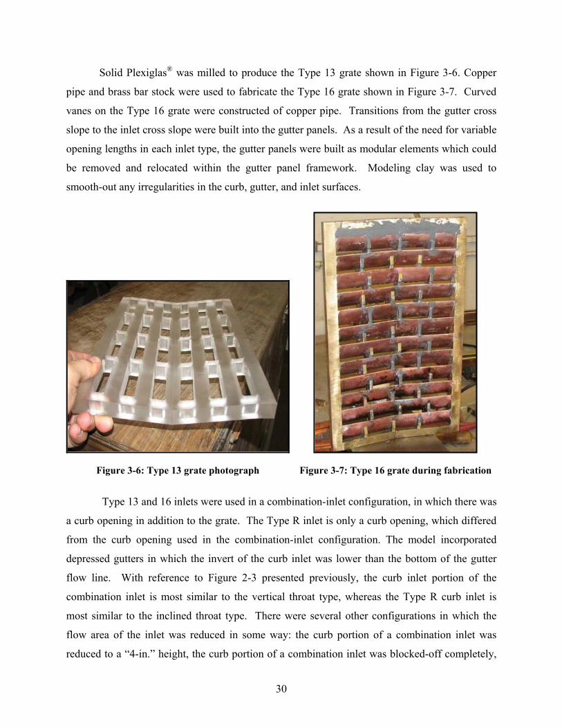
Solid Plexiglas® was milled to produce the Type 13 grate shown in Figure 3-6. Copper
pipe and brass bar stock were used to fabricate the Type 16 grate shown in Figure 3-7. Curved
vanes on the Type 16 grate were constructed of copper pipe. Transitions from the gutter cross
slope to the inlet cross slope were built into the gutter panels. As a result of the need for variable
opening lengths in each inlet type, the gutter panels were built as modular elements which could
be removed and relocated within the gutter panel framework. Modeling clay was used to
smooth-out any irregularities in the curb, gutter, and inlet surfaces.
Figure 3-6: Type 13 grate photograph Figure 3-7: Type 16 grate during fabrication
Type 13 and 16 inlets were used in a combination-inlet configuration, in which there was
a curb opening in addition to the grate. The Type R inlet is only a curb opening, which differed
from the curb opening used in the combination-inlet configuration. The model incorporated
depressed gutters in which the invert of the curb inlet was lower than the bottom of the gutter
flow line. With reference to Figure 2-3 presented previously, the curb inlet portion of the
combination inlet is most similar to the vertical throat type, whereas the Type R curb inlet is
most similar to the inclined throat type. There were several other configurations in which the
flow area of the inlet was reduced in some way: the curb portion of a combination inlet was
reduced to a “4-in.” height, the curb portion of a combination inlet was blocked-off completely,
31
the grate portion of a combination inlet was obstructed with debris, the grate portion of a
combination inlet was blocked-off completely, or a horizontal safety bar was used across the
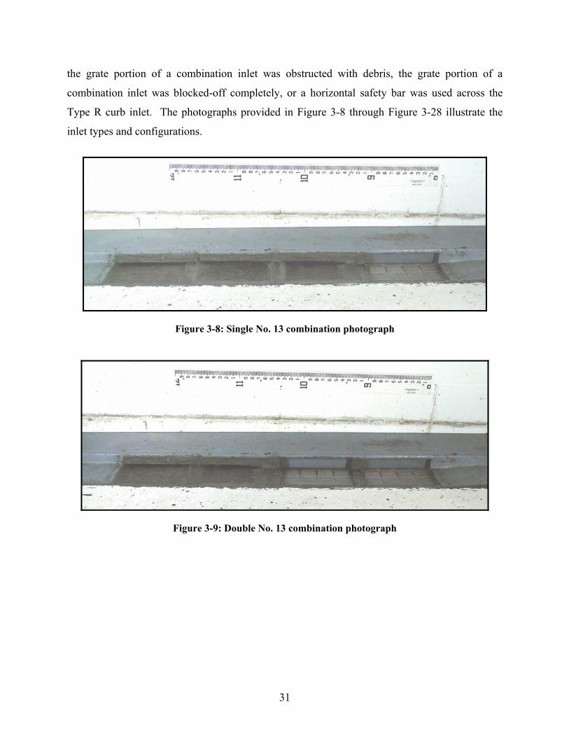
Type R curb inlet. The photographs provided in Figure 3-8 through Figure 3-28 illustrate the
inlet types and configurations.
Figure 3-8: Single No. 13 combination photograph
Figure 3-9: Double No. 13 combination photograph
32
Figure 3-10: Triple No. 13 combination photograph
Figure 3-11: Single No. 13 combination with 4-in. curb opening photograph
Figure 3-12: Single No. 13 combination with grate only photograph
Note Reducing
Plate
33
Figure 3-13: Single No. 13 curb opening only photograph
Figure 3-14: Single No. 13 combination debris test one photograph
Figure 3-15: Single No. 13 combination debris test two photograph
34
Figure 3-16: Single No. 16 combination photograph
Figure 3-17: Double No. 16 combination photograph
Figure 3-18: Triple No. 16 combination photograph
35
Figure 3-19: Single No. 16 with 4-in. curb opening photograph
Figure 3-20: Single No. 16 grate only photograph
Figure 3-21: Single No. 16 combination debris test one photograph
Note Reducing
Plate

36
Figure 3-22: Single No. 16 combination debris test two photograph
Figure 3-23: R5 curb inlet photograph
Figure 3-24: R9 curb inlet photograph
37
Figure 3-25: R12 curb inlet photograph
Figure 3-26: R15 curb inlet photograph
Figure 3-27: R5 with 4-in. curb opening photograph
Note Reducing
Plate

38
Figure 3-28: R5 with safety bar photograph
3.4 Model Operation and Testing Procedures A headbox was used to supply water to the model, a flume section contained the street
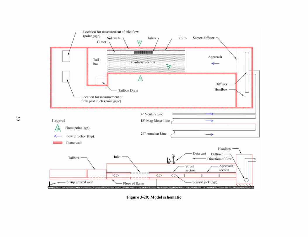
and inlet components, and a tailbox was used to catch flow that bypassed the inlets. Figure 3-29
provides a sketch of the entire model. Water flowed from the inlet valve to the headbox, through
the flume section, then exits into the tailbox. Two pumps fed water to the headbox through a
network of large pipes and valves. A 40-horsepower (hp) pump was used for the 0.33-ft and
0.50-ft prototype-scale depths, and a 75-hp pump was used for the 1-ft prototype-scale flow
depth. Both pumps drew water from a sump located beneath the laboratory floor, which was
approximately 1 acre ft in volume. Lined channels below the flume conveyed flow away from
the tailbox and back into the sump.
Note Safety
Bar
39
Figure 3-29: Model schematic

40
Flow entering and exiting the model was measured as part of the data-collection process.
Flow entered the model headbox through pipes as pressurized flow. Measurement-instrument
selection for inflow was based on the anticipated flow required for each test, and the associated
pump and pipelines used. Two instruments were used: 1) a differential pressure meter (annubar)
manufactured by the Rosemount division of the Emerson Process Management Company, and 2)
an electro-magnetic flow meter (mag meter) manufactured by the Endress and Hauser Company.
Table 3-7 summarizes flow-measurement characteristics of each instrument.
Table 3-7: Discharge measurement-instrument ranges
Instrument Type Flow Range (cfs)
Pipeline (in.)
Pump (hp)
Accuracy (%)
mag meter 0.13 - 10 18 40 0.5 annubar 6.5 - 15 24 75 2.5
Outflow from the model flume section was either conveyed through the inlets or
bypassed off the road section. In either case, the flow passed through an opening in the tailbox
of the flume and into channels below. Flow exiting the channels was measured by either a
rectangular weir for bypassed flow or V-notch sharp-crested weir for inlet captured flow. Both
weirs were constructed in accordance with published specifications (Bos, 1989; USBR, 2001).
Calibration was performed for each weir prior to testing of the model. Rating equations in the
form of Equation 3-1 were developed by regression analysis of depth-flow data over the
expected operating range of each weir. Coefficients and exponents used in these equations are
given in Table 3-8. For slope configurations greater than 0.5% longitudinal, the tailwater depth
was noted to rise significantly in the tailbox of the model. When this occurred, the weirs were
raised and recalibrated:
baHQ = Equation 3-1
where:
Q = discharge (cfs); a = coefficient of discharge; H = head above the weir crest (ft); and b = depth exponent.
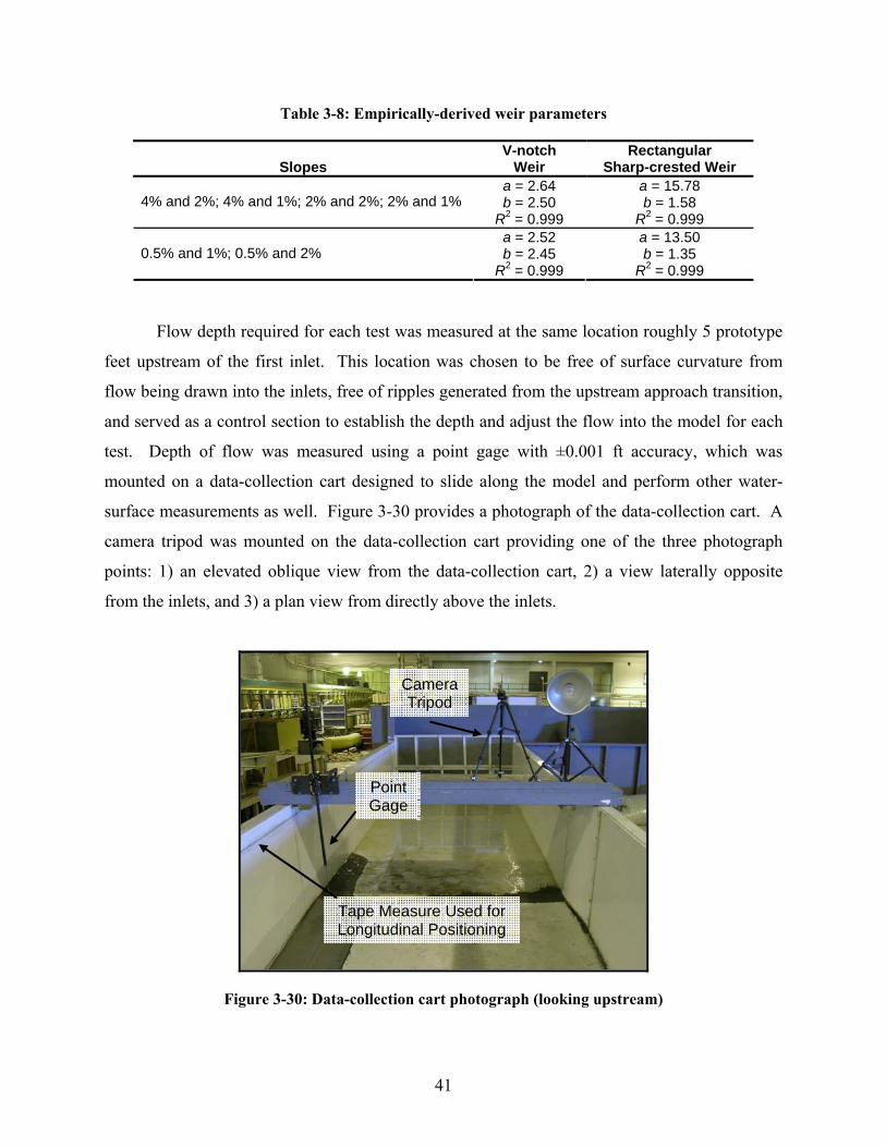
41
Table 3-8: Empirically-derived weir parameters
Slopes V-notch
Weir Rectangular
Sharp-crested Weir a = 2.64 a = 15.78 b = 2.50 b = 1.58 4% and 2%; 4% and 1%; 2% and 2%; 2% and 1%
R2 = 0.999 R2 = 0.999 a = 2.52 a = 13.50 b = 2.45 b = 1.35 0.5% and 1%; 0.5% and 2%
R2 = 0.999 R2 = 0.999
Flow depth required for each test was measured at the same location roughly 5 prototype
feet upstream of the first inlet. This location was chosen to be free of surface curvature from
flow being drawn into the inlets, free of ripples generated from the upstream approach transition,
and served as a control section to establish the depth and adjust the flow into the model for each
test. Depth of flow was measured using a point gage with ±0.001 ft accuracy, which was
mounted on a data-collection cart designed to slide along the model and perform other water-
surface measurements as well. Figure 3-30 provides a photograph of the data-collection cart. A
camera tripod was mounted on the data-collection cart providing one of the three photograph
points: 1) an elevated oblique view from the data-collection cart, 2) a view laterally opposite
from the inlets, and 3) a plan view from directly above the inlets.
Figure 3-30: Data-collection cart photograph (looking upstream)
Camera Tripod
Point Gage
Tape Measure Used for Longitudinal Positioning

42
Following a standardized testing procedure assured consistency and facilitated data
collection by multiple technicians. Prior to testing, the street slope and inlet type were
configured. The flow depth was then set on the point gage and the flow into the model was
adjusted to contact the point gage. Technicians waited approximately 10 minutes once the target
depth was achieved for flow conditions to stabilize. Outflow measurement point gages were
checked periodically during this time until the readings stabilized. Test conditions were then
checked and recorded on the data sheet. If the slope and inlet configurations did not change for a
subsequent test, a new depth was set on the point gage and the flow adjusted accordingly. If a
new slope or inlet configuration was required, the pumps were shut off and the model was
reconfigured. If the spread of water did not cover the street section for any given test, the extent
of flow was recorded to provide a top width at every longitudinal station. A fixed measuring
tape was used to determine longitudinal stations along the flume. Lateral positions across the
flume were determined with a measuring tape affixed to the data-collection cart. Both tapes
were graduated in tenths of a foot and had ±0.01 ft accuracy.
Data collection was documented by completing a data sheet for each test, taking still
photographs, and shooting short videos. The data-collection sheet used for all testing is
presented in Appendix E. Data collection was comprised of the following information: date,
operator name, water temperature, test ID number, start and end times, slope configuration, inlet
configuration, discharge and measurement devices used, depth of flow, extent of flow, and flow
characteristics. Flow characteristics consisted of any general observations that the operator
recorded for a particular test. Typical observations included the condition of flow around the
inlets (if waves emanated or splashing occurred), and if possible an approximation of flow
percentage passing through each inlet was made.
Several measures were taken to maintain data quality. After the testing procedures
described above were followed, data were entered into the database by the operator, and then
checked by another person for accuracy with the original data sheets. A survey of the model was
performed every time the model inlet type was changed. This confirmed that the model was not
shifting or settling, and that the slope was accurate to within allowable limits of 0.05% for
longitudinal and cross slopes.
43
3.5 Summary A testing program designed for evaluating the performance of Type 13, 16, and R inlets,
comprised of 318 tests, was conducted at Colorado State University. A 1/3-scale model of a
two-lane street section was constructed. Variations in street longitudinal slope, cross slope, inlet
length, and flow depth were accomplished to provide data on captured inlet flow and bypassed
street flow. In addition, the spread of flow was measured along the street section. Surface
roughness of the prototype was designed to be 0.015, which is the mean value for asphalt.
Inflow to the model was measured using either a magnetic flow meter or a differential pressure
meter. Outflow from the model was measured using sharp-crested weirs for captured inlet flow
and bypassed street flow. Photographs were taken and video recordings were made to facilitate
later inspection of flow conditions in the model. From the collected test data, qualitative and
quantitative observations will be made for determination of efficiency for each inlet.

44

45
4 DATA AND OBSERVATIONS
Testing results presented in this report have been collected using the previously described
test procedures and quality control (QC) measures, and are presented at the prototype scale. The
large quantity of data is presented in this section in graphical form, organized by inlet type, and
qualitative observations are made concerning the performance of the Type 13, 16, and R inlets.
Sample tables of on-grade and sump test data are also presented. The entire collected test data
set is presented in tabular form in Appendices B and C, where it is organized by: test ID number,
inlet configuration, slopes, flow depth, total flow, efficiency, top width of flow at the upstream
control section, and top width of flow downstream of the inlets.
4.1 On-grade Tests A tabular sample of the on-grade test data is presented as Table 4-1. The entire on-grade
data set in included as Appendix B. Inlet efficiency was determined as the ratio of captured flow
to total street flow for each test as shown in Equation 4-1:
100×=flowstreettotal
flowinletcapturedE Equation 4-1
where:
E = inlet efficiency (%).

46
Table 4-1: Sample on-grade test data
Test ID Number
Configuration
Longitudinal Slope
(%)
Cross Slope
(%)
Flow Depth
(ft)
Prototype Total Flow (cfs)
Efficiency (%)
Top Width
at Control
(ft)
Top Width Downstream
of Inlets (ft)
56 Triple No. 13 0.5 1 0.333 4.4 82.1 15.8 9.0 57 Triple No. 13 0.5 1 0.501 20.6 43.2 18.2 18.2 58 Triple No. 13 0.5 1 0.999 126.6 22.7 18.2 18.2 59 Double No. 13 0.5 1 0.333 4.7 73.3 16.0 10.7 60 Double No. 13 0.5 1 0.501 22.6 35.9 18.2 18.2 61 Double No. 13 0.5 1 0.999 127.8 16.2 18.2 18.2 62 Single No. 13 0.5 1 0.333 4.8 61.3 16.0 15.8 63 Single No. 13 0.5 1 0.501 26.2 23.8 18.2 18.2 64 Single No. 13 0.5 1 0.999 126.4 9.9 18.2 18.2
For illustration purposes, trend lines are fitted to the on-grade test data (as second-order
polynomials) in Figure 4-1 through Figure 4-3. Each trend line illustrates how efficiency
increases with increasing inlet length. Velocity was chosen as the independent variable in these
figures because of its significant effect on inlet efficiency.
Figure 4-1: Type 13 combination-inlet on-grade test data

47
Figure 4-2: Type 16 combination-inlet on-grade test data
Figure 4-3: Type R curb inlet on-grade test data
Several general trends can be found in the on-grade test data:
• The highest inlet efficiency occurs at the lowest flow velocity.
• The velocity of flow is influenced by the longitudinal and cross slopes, and lower
slopes produce lower velocity.
• Flow on the model street section was almost always supercritical
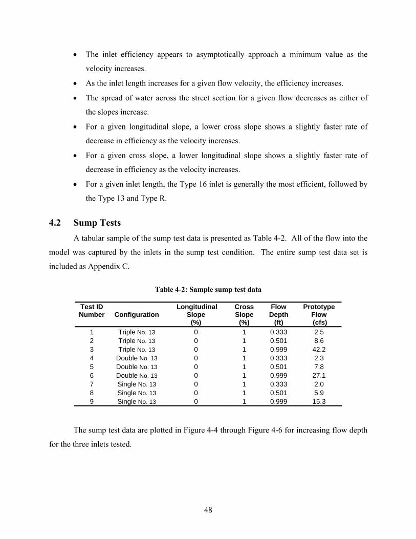
48
• The inlet efficiency appears to asymptotically approach a minimum value as the
velocity increases.
• As the inlet length increases for a given flow velocity, the efficiency increases.
• The spread of water across the street section for a given flow decreases as either of
the slopes increase.
• For a given longitudinal slope, a lower cross slope shows a slightly faster rate of
decrease in efficiency as the velocity increases.
• For a given cross slope, a lower longitudinal slope shows a slightly faster rate of
decrease in efficiency as the velocity increases.
• For a given inlet length, the Type 16 inlet is generally the most efficient, followed by
the Type 13 and Type R.
4.2 Sump Tests
A tabular sample of the sump test data is presented as Table 4-2. All of the flow into the
model was captured by the inlets in the sump test condition. The entire sump test data set is
included as Appendix C.
Table 4-2: Sample sump test data
Test ID Number
Configuration
Longitudinal Slope
(%)
Cross Slope
(%)
Flow Depth
(ft)
Prototype Flow (cfs)
1 Triple No. 13 0 1 0.333 2.5 2 Triple No. 13 0 1 0.501 8.6 3 Triple No. 13 0 1 0.999 42.2 4 Double No. 13 0 1 0.333 2.3 5 Double No. 13 0 1 0.501 7.8 6 Double No. 13 0 1 0.999 27.1 7 Single No. 13 0 1 0.333 2.0 8 Single No. 13 0 1 0.501 5.9 9 Single No. 13 0 1 0.999 15.3
The sump test data are plotted in Figure 4-4 through Figure 4-6 for increasing flow depth
for the three inlets tested.
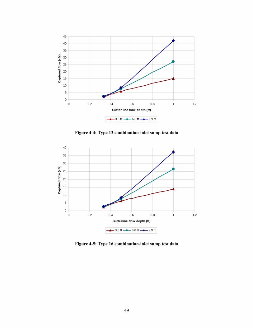
49
0
5
10
15
20
25
30
35
40
45
0 0.2 0.4 0.6 0.8 1 1.2
Gutter line flow depth (ft)
Cap
ture
d flo
w (c
fs)
3.3 f t 6.6 ft 9.9 ft
Figure 4-4: Type 13 combination-inlet sump test data
0
5
10
15
20
25
30
35
40
0 0.2 0.4 0.6 0.8 1 1.2
Gutterline flow depth (ft)
Cap
ture
d flo
w (c
fs)
3.3 ft 6.6 ft 9.9 ft
Figure 4-5: Type 16 combination-inlet sump test data
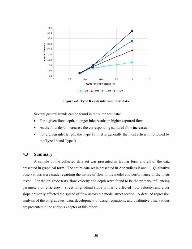
50
0.0
5.0
10.0
15.0
20.0
25.0
30.0
35.0
40.0
45.0
0 0.2 0.4 0.6 0.8 1 1.2
Gutterline flow depth (ft)
Cap
ture
d flo
w (c
fs)
5 ft 9 ft 12 ft 15 ft
Figure 4-6: Type R curb inlet sump test data
Several general trends can be found in the sump test data:
• For a given flow depth, a longer inlet results in higher captured flow.
• As the flow depth increases, the corresponding captured flow increases.
• For a given inlet length, the Type 13 inlet is generally the most efficient, followed by
the Type 16 and Type R.
4.3 Summary A sample of the collected data set was presented in tabular form and all of the data
presented in graphical form. The entire data set in presented in Appendices B and C. Qualitative
observations were made regarding the nature of flow in the model and performance of the inlets
tested. For the on-grade tests, flow velocity and depth were found to be the primary influencing
parameters on efficiency. Street longitudinal slope primarily affected flow velocity, and cross
slope primarily affected the spread of flow across the model street section. A detailed regression
analysis of the on-grade test data, development of design equations, and qualitative observations
are presented in the analysis chapter of this report.

51
5 ANALYSIS AND RESULTS
Data selected for analysis consisted of the unobstructed, on-grade configuration tests for
Type 13 and 16 combination inlets and the Type R curb inlet. Analysis presented in this chapter
is intended to provide improved methods for determining the efficiency of Type 13, 16, and R
inlets in the on-grade configuration. Included in the unobstructed, on-grade, test category is 180
out of 318 tests. Remaining test data including sump tests and debris tests will be analyzed by
other participating agencies. Presented in this chapter is a comparison between the observed
inlet efficiency from testing, inlet efficiency determined from current and improved UDFCD
calculation methods, and inlet efficiency determined from independent empirical equations
developed using the process of dimensional analysis. Presented in Figure 5-1 is a flow chart
illustrating the analysis. Empirical equations developed are intended to provide an independent
alternative to the UDFCD methods for determining inlet efficiency. Also examined in this
analysis is the relevance of achieving uniform flow in the model and a comparison is made
between combination and grate inlet performance for the Type 13 and 16 inlets.
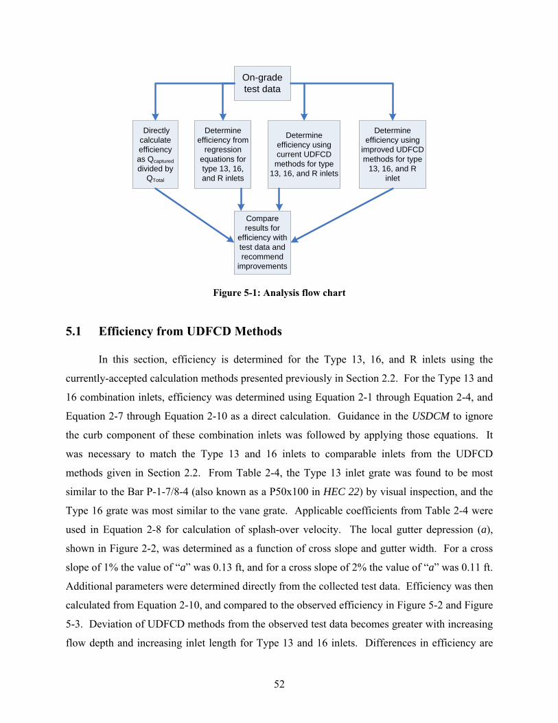
52
On-grade test data
Determine efficiency using current UDFCD methods for type
13, 16, and R inlets
Determine efficiency from
regression equations for type 13, 16, and R inlets
Determine efficiency using
improved UDFCD methods for type
13, 16, and R inlet
Directly calculate efficiency as Qcaptured divided by
QTotal
Compare results for
efficiency with test data and recommend
improvements
Figure 5-1: Analysis flow chart
5.1 Efficiency from UDFCD Methods
In this section, efficiency is determined for the Type 13, 16, and R inlets using the
currently-accepted calculation methods presented previously in Section 2.2. For the Type 13 and
16 combination inlets, efficiency was determined using Equation 2-1 through Equation 2-4, and
Equation 2-7 through Equation 2-10 as a direct calculation. Guidance in the USDCM to ignore
the curb component of these combination inlets was followed by applying those equations. It
was necessary to match the Type 13 and 16 inlets to comparable inlets from the UDFCD
methods given in Section 2.2. From Table 2-4, the Type 13 inlet grate was found to be most
similar to the Bar P-1-7/8-4 (also known as a P50x100 in HEC 22) by visual inspection, and the
Type 16 grate was most similar to the vane grate. Applicable coefficients from Table 2-4 were
used in Equation 2-8 for calculation of splash-over velocity. The local gutter depression (a),
shown in Figure 2-2, was determined as a function of cross slope and gutter width. For a cross
slope of 1% the value of “a” was 0.13 ft, and for a cross slope of 2% the value of “a” was 0.11 ft.
Additional parameters were determined directly from the collected test data. Efficiency was then
calculated from Equation 2-10, and compared to the observed efficiency in Figure 5-2 and Figure
5-3. Deviation of UDFCD methods from the observed test data becomes greater with increasing
flow depth and increasing inlet length for Type 13 and 16 inlets. Differences in efficiency are

53
likely due to the nature of the original FHWA test data used to develop Equation 2-4 through
Equation 2-10 for grate inlets. The FHWA study, summarized in Section 2.1, only tested to a
maximum flow depth of 0.45 ft and a maximum inlet length of 4 ft. Therefore, the data would
have had to be extrapolated to greater depths and inlet lengths. Analysis of the observed test data
presented here does not extrapolate beyond the actual conditions tested.
0
0.1
0.2
0.3
0.4
0.5
0.6
0.7
0.8
0.9
1
0 0.1 0.2 0.3 0.4 0.5 0.6 0.7 0.8 0.9 1
Predicted
Obs
erve
d
1 ft depth0.5 ft depth0.33 ft depthEqual
R2 Average efficiency error (%) Maximum efficiency error (%)
0.719 18.8 34.0
Figure 5-2: Predicted vs. observed efficiency for Type 13 combination inlet from UDFCD methods

54
0
0.1
0.2
0.3
0.4
0.5
0.6
0.7
0.8
0.9
1
0 0.1 0.2 0.3 0.4 0.5 0.6 0.7 0.8 0.9 1
Predicted
Obs
erve
d
1 ft depth0.5 ft depth0.33 ft depthEqual
`
R2 Average efficiency error (%) Maximum efficiency error (%)
0.574 17.7 39.0
Figure 5-3: Predicted vs. observed efficiency for Type 16 combination inlet from UDFCD methods
For the Type R curb inlet, efficiency was determined using Equation 2-11, Equation 2-13,
and Equation 2-14 as a direct calculation. Efficiency comparison with the observed test data is
presented in Figure 5-4, where agreement is best for high flow depths. Measured top width,
velocity, and cross-sectional flow area for each inlet test were used in the calculations and are
provided in Appendix F. Accuracy of these methods for the Type 13, 16, and R inlets will be
improved in Section 5.2 when the UDFCD methods are extended to include them directly.

55
0
0.1
0.2
0.3
0.4
0.5
0.6
0.7
0.8
0.9
1
0 0.1 0.2 0.3 0.4 0.5 0.6 0.7 0.8 0.9 1
Predicted
Obs
erve
d
1 ft depth0.5 ft depth0.33 ft depthEqual
R2 Average efficiency error (%) Maximum efficiency error (%)
0.861 6.5 30.2
Figure 5-4: Predicted vs. observed efficiency for Type R curb inlet from UDFCD methods
For the most similar inlets to the Type 13 and 16 combination inlets currently available in
the USDCM, the UDFCD methods over-predict efficiency by an average of about 20%. For the
most similar inlet to the Type R curb inlet currently available in the USDCM, the UDFCD
methods generally under-predict efficiency by an average of 7%. These predictions can be
improved by slight modification of the currently-accepted design methods.
5.2 Improvements to UDFCD Efficiency Calculation Methods
One of the research objectives of this study was to extend the UDFCD methods for
determining inlet efficiency to include the Type 13 and 16 inlets, and to improve methods for the
Type R curb inlet. From the plots presented in Section 5.1, it can be seen that efficiency was
generally over-predicted for the combination inlets and under-predicted for the curb inlet. For
grate-type inlets, the only equation given in the USDCM that is grate-specific was presented
previously as Equation 2-8 for calculating splash-over velocity (Vo). Coefficients used in the
third-order polynomial of Equation 2-8 to calculate Vo are what need to be developed for the
Type 13 and 16 inlets. Splash-over velocity is a unique value for a given grate type and length.
By inspection of testing photographs and recorded videos, it was concluded that flow velocity in
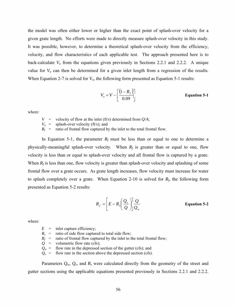
56
the model was often either lower or higher than the exact point of splash-over velocity for a
given grate length. No efforts were made to directly measure splash-over velocity in this study.
It was possible, however, to determine a theoretical splash-over velocity from the efficiency,
velocity, and flow characteristics of each applicable test. The approach presented here is to
back-calculate Vo from the equations given previously in Sections 2.2.1 and 2.2.2. A unique
value for Vo can then be determined for a given inlet length from a regression of the results.
When Equation 2-7 is solved for Vo, the following form presented as Equation 5-1 results:
( )
⎥⎦
⎤⎢⎣
⎡ −−=
0901
.R
VV fo Equation 5-1
where:
V = velocity of flow at the inlet (ft/s) determined from Q/A; Vo = splash-over velocity (ft/s); and Rf = ratio of frontal flow captured by the inlet to the total frontal flow.
In Equation 5-1, the parameter Rf must be less than or equal to one to determine a
physically-meaningful splash-over velocity. When Rf is greater than or equal to one, flow
velocity is less than or equal to splash-over velocity and all frontal flow is captured by a grate.
When Rf is less than one, flow velocity is greater than splash-over velocity and splashing of some
frontal flow over a grate occurs. As grate length increases, flow velocity must increase for water
to splash completely over a grate. When Equation 2-10 is solved for Rf, the following form
presented as Equation 5-2 results:
w
ssf Q
QQQ
RER ⎥⎦
⎤⎢⎣
⎡⎟⎟⎠
⎞⎜⎜⎝
⎛−= Equation 5-2
where:
E = inlet capture efficiency; Rs = ratio of side flow captured to total side flow; Rf = ratio of frontal flow captured by the inlet to the total frontal flow; Q = volumetric flow rate (cfs); Qw = flow rate in the depressed section of the gutter (cfs); and Qs = flow rate in the section above the depressed section (cfs).
Parameters Qw, Qs, and Rs were calculated directly from the geometry of the street and
gutter sections using the applicable equations presented previously in Sections 2.2.1 and 2.2.2.
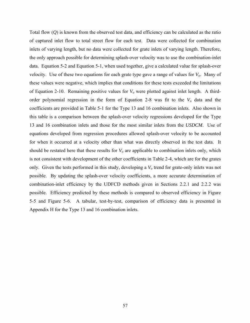
57
Total flow (Q) is known from the observed test data, and efficiency can be calculated as the ratio
of captured inlet flow to total street flow for each test. Data were collected for combination
inlets of varying length, but no data were collected for grate inlets of varying length. Therefore,
the only approach possible for determining splash-over velocity was to use the combination-inlet
data. Equation 5-2 and Equation 5-1, when used together, give a calculated value for splash-over
velocity. Use of these two equations for each grate type gave a range of values for Vo. Many of
these values were negative, which implies that conditions for these tests exceeded the limitations
of Equation 2-10. Remaining positive values for Vo were plotted against inlet length. A third-
order polynomial regression in the form of Equation 2-8 was fit to the Vo data and the
coefficients are provided in Table 5-1 for the Type 13 and 16 combination inlets. Also shown in
this table is a comparison between the splash-over velocity regressions developed for the Type
13 and 16 combination inlets and those for the most similar inlets from the USDCM. Use of
equations developed from regression procedures allowed splash-over velocity to be accounted
for when it occurred at a velocity other than what was directly observed in the test data. It
should be restated here that these results for Vo are applicable to combination inlets only, which
is not consistent with development of the other coefficients in Table 2-4, which are for the grates
only. Given the tests performed in this study, developing a Vo trend for grate-only inlets was not
possible. By updating the splash-over velocity coefficients, a more accurate determination of
combination-inlet efficiency by the UDFCD methods given in Sections 2.2.1 and 2.2.2 was
possible. Efficiency predicted by these methods is compared to observed efficiency in Figure
5-5 and Figure 5-6. A tabular, test-by-test, comparison of efficiency data is presented in
Appendix H for the Type 13 and 16 combination inlets.

58
Table 5-1: Updated splash-over velocity coefficients and plots
Grate α β γ η R2 Type 13 0 0.583 0.030 0.0001 0.43 Type 16 0 0.815 0.074 0.0024 0.24
where: 32eeeo LLLV ηγβα +−+=
Type 13 grate inlet
02468
101214161820
0 2 4 6 8 10
Grate length (ft)
Spl
asho
ver
velo
city
(ft/s
)
USDCMTest data
Type 16 grate inlet
02468
101214161820
0 2 4 6 8 10
Grate length (ft)
Spla
shov
er v
eloc
ity (f
t/s)
USDCMTest data
59
0
0.1
0.2
0.3
0.4
0.5
0.6
0.7
0.8
0.9
1
0 0.1 0.2 0.3 0.4 0.5 0.6 0.7 0.8 0.9 1
Predicted
Obs
erve
d
1 ft depth0.5 ft depth0.33 ft depthEqual
1
R2 Average efficiency error (%) Maximum efficiency error (%) 0.804 8.6 31.0
Figure 5-5: Predicted vs. observed efficiency for Type 13 combination inlet from improved UDFCD methods
0
0.1
0.2
0.3
0.4
0.5
0.6
0.7
0.8
0.9
1
0 0.1 0.2 0.3 0.4 0.5 0.6 0.7 0.8 0.9 1
Predicted
Obs
erve
d
1 ft depth0.5 ft depth0.33 ft depthEqual
R2 Average efficiency error (%) Maximum efficiency error (%) 0.644 13.6 39.0
Figure 5-6: Predicted vs. observed efficiency for Type 16 combination inlet from improved UDFCD methods
60
Efficiency for the Type R curb inlet presented in Section 5.1 was calculated from
Equation 2-11 and Equation 2-13. Calculated efficiency from these two equations can be
improved by updating the coefficient and exponents of Equation 2-13. By doing this, the
original form of the equation is preserved. Equation 5-3 illustrates the general form of this
equation, where the coefficient N and the exponents a, b, and c will be determined by regression
of the test data:
c
e
bL
aT nS
SNQL ⎟⎟⎠
⎞⎜⎜⎝
⎛=
1 Equation 5-3
where:
LT = curb opening length required to capture 100% of gutter flow; Q = gutter flow (cfs); SL = longitudinal street slope (ft/ft); Se = equivalent street cross slope (ft/ft); n = Manning’s roughness coefficient; N = regression coefficient; and a,b,c = regression exponents.
The improved results of using Equation 5-3 to determine efficiency are presented in
Figure 5-7. A tabular test-by-test comparison is presented in Appendix B for the Type R curb
inlet. The final form of this equation is presented as Equation 5-4:
0.46
0.51 0.058 10.38T Le
L Q SnS
⎛ ⎞= ⎜ ⎟
⎝ ⎠ Equation 5-4

61
0
0.1
0.2
0.3
0.4
0.5
0.6
0.7
0.8
0.9
1
0 0.1 0.2 0.3 0.4 0.5 0.6 0.7 0.8 0.9 1
Predicted
Obs
erve
d
1 ft depth0.5 ft depth0.33 ft depthEqual
R2 Average efficiency error (%) Maximum efficiency error (%)
0.948 3.8 15.7
Figure 5-7: Predicted vs. observed efficiency for Type R curb inlet from improved UDFCD methods
Efficiency predictions by the UDFCD methods were improved slightly for each of the
inlets tested. The methods were extended to include the Type 13 and 16 combination inlets, with
efficiency over-predicted by an average of 10%. For these inlets, agreement with observed test
data is still best at low flow depth. For the Type R curb inlet, UDFCD methods were modified
slightly, and efficiency error spread evenly at 3.8%. Agreement is still best at higher flow
depths, and has been improved for the lowest depth. Efficiency predictions can be further
improved by developing new empirical relationships for each inlet.
5.3 Efficiency from Dimensional Analysis and Empirical Equations
In this section empirical equations are presented, as an alternative to the use of the
UDFCD methods, for determination of inlet efficiency for the Type 13 combination, Type 16
combination, and Type R curb inlets. Equations presented will provide a simpler and more
accurate method, than that presented in the USDCM, for determining efficiency in the on-grade
condition. Methods presented in the USDCM suffer from, in part, use of theoretical parameters
that can not be physically determined by a user (such as splash-over velocity, Rf, Rs, Qw, and Qs).
62
From a design perspective, a user approaching an inlet design situation will know several
parameters: street flow (and velocity from continuity), design flow depth (and area), allowable
spread of flow, street longitudinal slope, and street cross slope. Given values for those
parameters, a suitable inlet length is typically sought that provides an acceptable degree of flow
capture efficiency for a particular street location. A desirable equation will utilize physically-
known parameters in a form that is easily applied to determine efficiency.
It was possible to develop one equation for each inlet type to predict the basic on-grade
test data. Power regression equations were used because of their easy integration with
dimensional analysis, which was described as the process of selecting parameter groups for use
in equation development. Application of dimensional analysis began with simply identifying the
parameters of interest. Parameters typically known or desired by a designer are re-stated in
functional form as:
),,,,,,( TAhLVSSfE Lc= Equation 5-5
where:
E = inlet capture efficiency; Sc = cross slope; SL = longitudinal slope; V = velocity (ft/s); L = grate or inlet length (ft); h = depth of flow in the gutter (ft); A = flow area (ft2); and T = top width of flow spread from the curb face (ft).
Calculation of values for parameters in Equation 5-5 was necessary for each test, and
they are given in Appendix F by test number. Parameters in Equation 5-5 were arranged into
dimensionless groups (called Pi groups) using the Buckingham Pi theorem described previously
in Section 2.5. Units were made consistent in several dimensionless groups by use of the
gravitational constant (g). Applying the Buckingham Pi theorem, with repeating variables of V
and h or V and L, resulted in the following dimensionless parameter groups:
ESSgLV
ghV
gATV
Lh
lc =Π=Π=Π=Π=Π=Π=Π 765
2
4
2
3
2
21 ,,,,,,

63
The second Pi group is the square of the Froude number for a general channel cross
section, and the third Pi group is the Froude number for a rectangular channel. Both forms of the
Froude number were tested for statistical significance, and either form was used in the final
equations. Compiling the Pi groups into power-equation form resulted in Equation 5-6:
( ) ( ) fl
ec
dcba
SSgLV
ghV
gATV
LhNE ⎟⎟
⎠
⎞⎜⎜⎝
⎛⎟⎟⎠
⎞⎜⎜⎝
⎛⎟⎟⎠
⎞⎜⎜⎝
⎛⎟⎠⎞
⎜⎝⎛=
222
Equation 5-6
where:
N = coefficient of regression; a,b,c,d,e,f = regression exponents to be determined by statistical analysis of the test data;
and remaining parameters were defined previously.
The computer application Statistical Analysis Software (SAS) was used to efficiently
analyze the large amount of test data. Analysis was carried-out using the logarithms of each Pi
group so a multi-variable linear regression model could be fit to the data. Coefficients given by a
linear model for each independent variable are the exponents (a, b, c, d, e, and f) and the y-
intercept given is the logarithm of the coefficient N for the equivalent power-equation form, as
shown in Equation 5.7:
fedcbaN 7543216 ΠΠΠΠΠΠ=Π , or Equation 5-7
7543216 loglogloglogloglogloglog Π+Π+Π+Π+Π+Π+=Π fedcbaN
The Statistics Department at CSU was consulted to assist in examination of the
regression statistics from SAS. When a regression is performed using SAS, the significance of
each parameter is examined and the effect of each possible parameter combination on the
regression fit is tested. Significance of each parameter is evaluated by dividing the standard
error of the parameter estimate by the estimate itself. The result is called the “t” value and a
significant parameter has an absolute t value greater than 2 (i.e., the estimate itself is at least two
times larger than its error, and the 95% confidence interval for the estimate is two times the
standard error). The level of confidence that a parameter estimate has not arisen by chance
(called the significance level) is also evaluated by SAS and reported as the Pr value. A Pr value
64
less than 0.0001 (the minimum level reported by SAS) means that there is less than a one in ten
thousand chance that the parameter estimate could have arisen by chance. Parameter groups that
did not give a t value >2 and a Pr value <0.0001 were eliminated from the model for each inlet
type. The effect of each parameter group on the overall regression fit was examined by checking
the R2 value as different combinations of groups were used. By doing this, statistically-
significant parameter groups were combined in the best possible way to achieve the highest R2
value. Finally, the range of predicted values for the dependent variable was checked for outliers
by application of the Studentized residual test by SAS. A Studentized residual greater than three
is an indicator that a predicted value has exceeded three standard deviations from the mean
predicted value. No outliers were noted in the analysis.
Equations developed are presented in their parameter group form and a simplified form
determined by combining like terms. Final empirical equations and statistical summaries are
presented in Table 5-2. A detailed statistical analysis from SAS for each equation in linear form
is provided in Appendix G. Results from applying the empirical equations are plotted against the
observed test data for efficiency in Figure 5-8 through Figure 5-10. The long slope parameter
was not found to be statistically significant for any of the inlets. For the Type 13 and 16 inlets,
the general form of the Froude number was preferred over the rectangular form, and use of the
cross slope parameter was not necessary. For the Type R curb inlet, use of the first Pi group was
not necessary and no statistical advantage was achieved by use of the general form of the Froude
number, so the simplified form for a rectangular cross section was used. Tabular values of
efficiency determined from these equations for each test are provided in Appendix H.
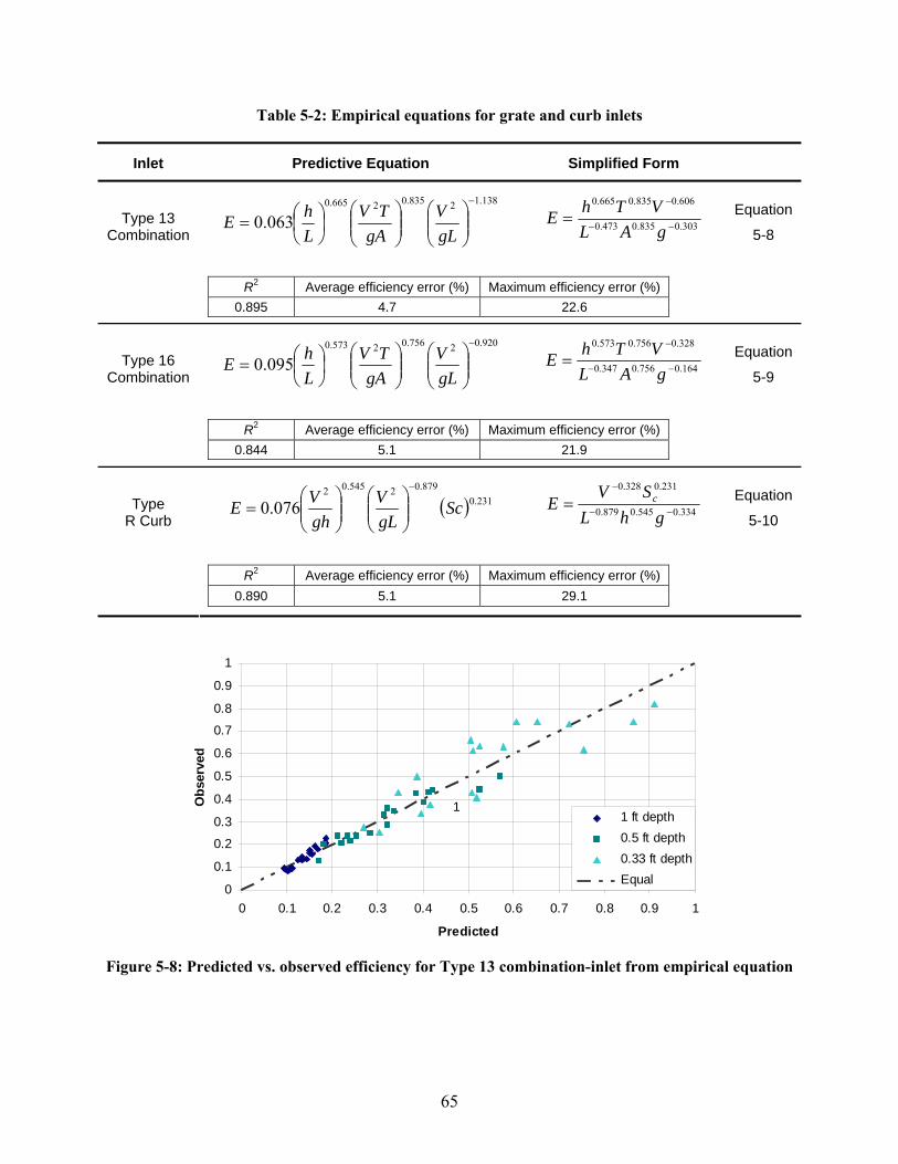
65
Table 5-2: Empirical equations for grate and curb inlets
Inlet Predictive Equation Simplified Form
138.12835.02665.0
063.0−
⎟⎟⎠
⎞⎜⎜⎝
⎛⎟⎟⎠
⎞⎜⎜⎝
⎛⎟⎠⎞
⎜⎝⎛=
gLV
gATV
LhE 303.0835.0473.0
606.0835.0665.0
−−
−
=gAL
VThE Equation
5-8
Type 13
Combination
R2 Average efficiency error (%) Maximum efficiency error (%) 0.895 4.7 22.6
920.02756.02573.0
095.0−
⎟⎟⎠
⎞⎜⎜⎝
⎛⎟⎟⎠
⎞⎜⎜⎝
⎛⎟⎠⎞
⎜⎝⎛=
gLV
gATV
LhE 164.0756.0347.0
328.0756.0573.0
−−
−
=gAL
VThE Equation
5-9
Type 16
Combination
R2 Average efficiency error (%) Maximum efficiency error (%) 0.844 5.1 21.9
( ) 231.0879.02545.02
076.0 ScgLV
ghVE
−
⎟⎟⎠
⎞⎜⎜⎝
⎛⎟⎟⎠
⎞⎜⎜⎝
⎛= 334.0545.0879.0
231.0328.0
−−
−
=ghL
SVE c Equation
5-10
Type
R Curb
R2 Average efficiency error (%) Maximum efficiency error (%) 0.890 5.1 29.1
0
0.1
0.2
0.3
0.4
0.5
0.6
0.7
0.8
0.9
1
0 0.1 0.2 0.3 0.4 0.5 0.6 0.7 0.8 0.9 1
Predicted
Obs
erve
d
1 ft depth0.5 ft depth0.33 ft depthEqual
1
Figure 5-8: Predicted vs. observed efficiency for Type 13 combination-inlet from empirical equation

66
0
0.1
0.2
0.3
0.4
0.5
0.6
0.7
0.8
0.9
1
0 0.1 0.2 0.3 0.4 0.5 0.6 0.7 0.8 0.9 1
Predicted
Obs
erve
d
1 ft depth0.5 ft depth0.33 ft depthEqual
Figure 5-9: Predicted vs. observed efficiency for Type 16 combination-inlet from empirical equation
0
0.1
0.2
0.3
0.4
0.5
0.6
0.7
0.8
0.9
1
0 0.1 0.2 0.3 0.4 0.5 0.6 0.7 0.8 0.9 1
Predicted
Obs
erve
d
1 ft depth0.5 ft depth0.33 ft depthEqual
Figure 5-10: Predicted vs. observed efficiency for Type R curb inlet from empirical equation
By developing new equations to predict efficiency, it was possible to further improve
predictions for inlet efficiency over previous sections. With new equations presented here, the
average error in predicted efficiency was reduced to about 5% for all inlets with R2 values
between 0.84 and 0.90. Overall agreement between observed and predicted efficiency is
improved over previous methods for all test depths. A comparison is shown in Figure 5-11
through Figure 5-13 between the empirical equations and the improved UDFCD methods.

67
Agreement is best at the smallest flow depth for the Type 13 and 16 inlets. This is due to the test
conditions of the original FHWA model described previously which only tested to a maximum
depth of 0.45 ft. For the Type R curb inlet, agreement is best at a high-flow depth.
0
0.1
0.2
0.3
0.4
0.5
0.6
0.7
0.8
0.9
1
0 0.1 0.2 0.3 0.4 0.5 0.6 0.7 0.8 0.9 1
UDFCD new
Em
piri
cal
1 ft depth0.5 ft depth0.33 ft depthEqual
1
Figure 5-11: Type 13 combination-inlet efficiency comparison
0
0.1
0.2
0.3
0.4
0.5
0.6
0.7
0.8
0.9
1
0 0.1 0.2 0.3 0.4 0.5 0.6 0.7 0.8 0.9 1
UDFCD new
Em
piri
cal
1 ft depth0.5 ft depth0.33 ft depthEqual
Figure 5-12: Type 16 combination-inlet efficiency comparison
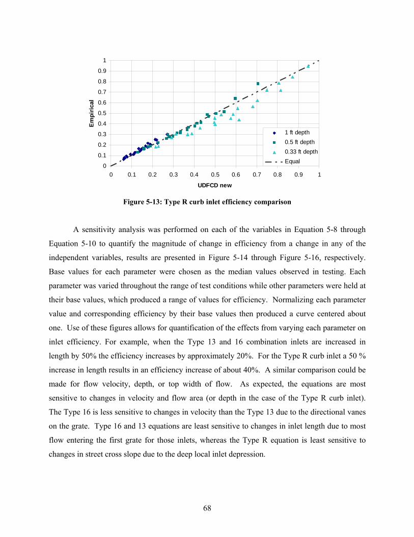
68
0
0.1
0.2
0.3
0.4
0.5
0.6
0.7
0.8
0.9
1
0 0.1 0.2 0.3 0.4 0.5 0.6 0.7 0.8 0.9 1
UDFCD new
Em
piri
cal
1 ft depth0.5 ft depth0.33 ft depthEqual
Figure 5-13: Type R curb inlet efficiency comparison
A sensitivity analysis was performed on each of the variables in Equation 5-8 through
Equation 5-10 to quantify the magnitude of change in efficiency from a change in any of the
independent variables, results are presented in Figure 5-14 through Figure 5-16, respectively.
Base values for each parameter were chosen as the median values observed in testing. Each
parameter was varied throughout the range of test conditions while other parameters were held at
their base values, which produced a range of values for efficiency. Normalizing each parameter
value and corresponding efficiency by their base values then produced a curve centered about
one. Use of these figures allows for quantification of the effects from varying each parameter on
inlet efficiency. For example, when the Type 13 and 16 combination inlets are increased in
length by 50% the efficiency increases by approximately 20%. For the Type R curb inlet a 50 %
increase in length results in an efficiency increase of about 40%. A similar comparison could be
made for flow velocity, depth, or top width of flow. As expected, the equations are most
sensitive to changes in velocity and flow area (or depth in the case of the Type R curb inlet).
The Type 16 is less sensitive to changes in velocity than the Type 13 due to the directional vanes
on the grate. Type 16 and 13 equations are least sensitive to changes in inlet length due to most
flow entering the first grate for those inlets, whereas the Type R equation is least sensitive to
changes in street cross slope due to the deep local inlet depression.
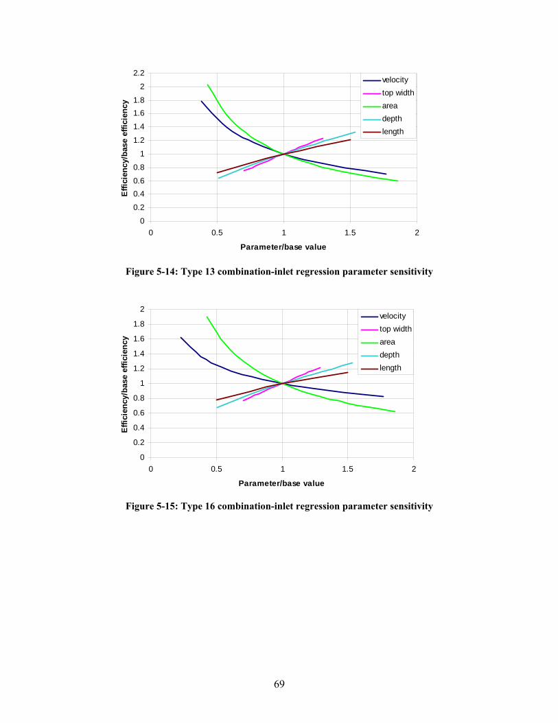
69
0
0.2
0.40.6
0.8
1
1.2
1.4
1.61.8
2
2.2
0 0.5 1 1.5 2
Parameter/base value
Effi
cien
cy/b
ase
effic
ienc
y
velocitytop widthareadepthlength
Figure 5-14: Type 13 combination-inlet regression parameter sensitivity
0
0.2
0.4
0.6
0.8
1
1.2
1.4
1.6
1.8
2
0 0.5 1 1.5 2
Parameter/base value
Effic
ienc
y/ba
se e
ffici
ency
velocitytop widthareadepthlength
Figure 5-15: Type 16 combination-inlet regression parameter sensitivity
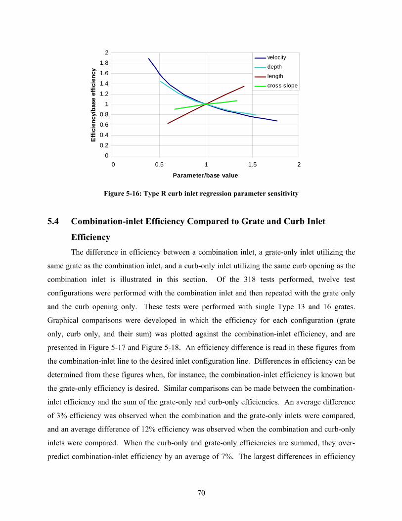
70
0
0.2
0.4
0.6
0.8
1
1.2
1.4
1.6
1.8
2
0 0.5 1 1.5 2
Parameter/base value
Effi
cien
cy/b
ase
effic
ienc
y
velocity
depth
length
cross slope
Figure 5-16: Type R curb inlet regression parameter sensitivity
5.4 Combination-inlet Efficiency Compared to Grate and Curb Inlet
Efficiency The difference in efficiency between a combination inlet, a grate-only inlet utilizing the
same grate as the combination inlet, and a curb-only inlet utilizing the same curb opening as the
combination inlet is illustrated in this section. Of the 318 tests performed, twelve test
configurations were performed with the combination inlet and then repeated with the grate only
and the curb opening only. These tests were performed with single Type 13 and 16 grates.
Graphical comparisons were developed in which the efficiency for each configuration (grate
only, curb only, and their sum) was plotted against the combination-inlet efficiency, and are
presented in Figure 5-17 and Figure 5-18. An efficiency difference is read in these figures from
the combination-inlet line to the desired inlet configuration line. Differences in efficiency can be
determined from these figures when, for instance, the combination-inlet efficiency is known but
the grate-only efficiency is desired. Similar comparisons can be made between the combination-
inlet efficiency and the sum of the grate-only and curb-only efficiencies. An average difference
of 3% efficiency was observed when the combination and the grate-only inlets were compared,
and an average difference of 12% efficiency was observed when the combination and curb-only
inlets were compared. When the curb-only and grate-only efficiencies are summed, they over-
predict combination-inlet efficiency by an average of 7%. The largest differences in efficiency

71
were typically seen at higher flow depths when the inlets became submerged. Performing
similar comparisons for two and three grates would be useful, but no data were collected for
configurations consisting of more than one grate or curb inlet. At lower flow depths (where flow
is entirely below the curb) for multiple curb openings, little difference would likely be seen due
to the observation that, at lower depths, almost no flow enters through the second and third curb
openings in the combination-inlet configuration. At higher flows (where the flow is at or above
the curb) all curb openings are expected to contribute significantly due to submergence, and the
difference in efficiency could be greater.
0
10
20
30
40
50
60
0 5 10 15 20 25 30 35 40
Observed combination Efficiency
obse
rved
eff
icie
ncy
sumgratecurbcombinationP ( )
Figure 5-17: Type 13 inlet configurations and efficiency
0
10
20
30
40
50
60
0 5 10 15 20 25 30 35 40
Observed combination Efficiency
Obs
erve
d ef
ficie
ncy
sumgratecurbcombination
Figure 5-18: Type 16 inlet configurations and efficiency
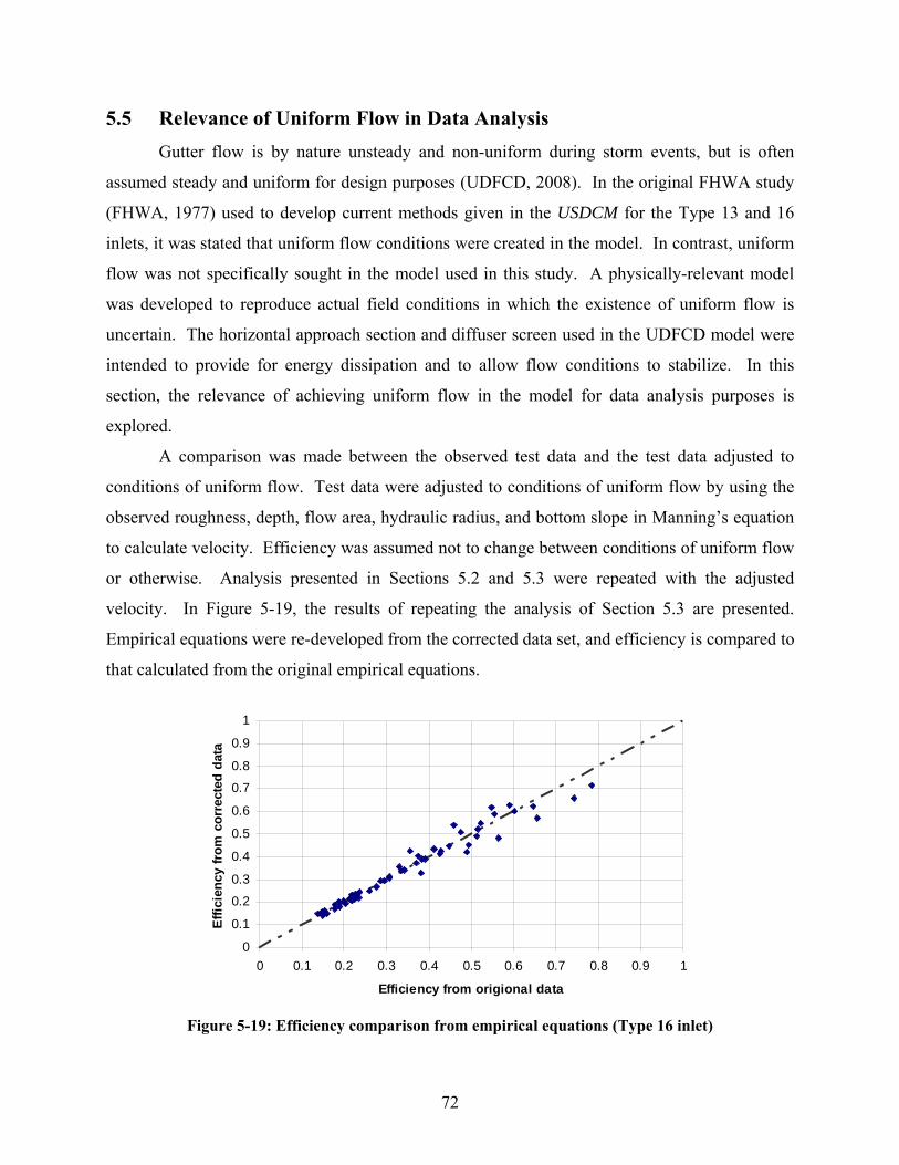
72
5.5 Relevance of Uniform Flow in Data Analysis Gutter flow is by nature unsteady and non-uniform during storm events, but is often
assumed steady and uniform for design purposes (UDFCD, 2008). In the original FHWA study
(FHWA, 1977) used to develop current methods given in the USDCM for the Type 13 and 16
inlets, it was stated that uniform flow conditions were created in the model. In contrast, uniform
flow was not specifically sought in the model used in this study. A physically-relevant model
was developed to reproduce actual field conditions in which the existence of uniform flow is
uncertain. The horizontal approach section and diffuser screen used in the UDFCD model were
intended to provide for energy dissipation and to allow flow conditions to stabilize. In this
section, the relevance of achieving uniform flow in the model for data analysis purposes is
explored.
A comparison was made between the observed test data and the test data adjusted to
conditions of uniform flow. Test data were adjusted to conditions of uniform flow by using the
observed roughness, depth, flow area, hydraulic radius, and bottom slope in Manning’s equation
to calculate velocity. Efficiency was assumed not to change between conditions of uniform flow
or otherwise. Analysis presented in Sections 5.2 and 5.3 were repeated with the adjusted
velocity. In Figure 5-19, the results of repeating the analysis of Section 5.3 are presented.
Empirical equations were re-developed from the corrected data set, and efficiency is compared to
that calculated from the original empirical equations.
0
0.1
0.2
0.3
0.4
0.5
0.6
0.7
0.8
0.9
1
0 0.1 0.2 0.3 0.4 0.5 0.6 0.7 0.8 0.9 1
Efficiency from origional data
Effic
ienc
y fro
m c
orre
cted
dat
a
Figure 5-19: Efficiency comparison from empirical equations (Type 16 inlet)
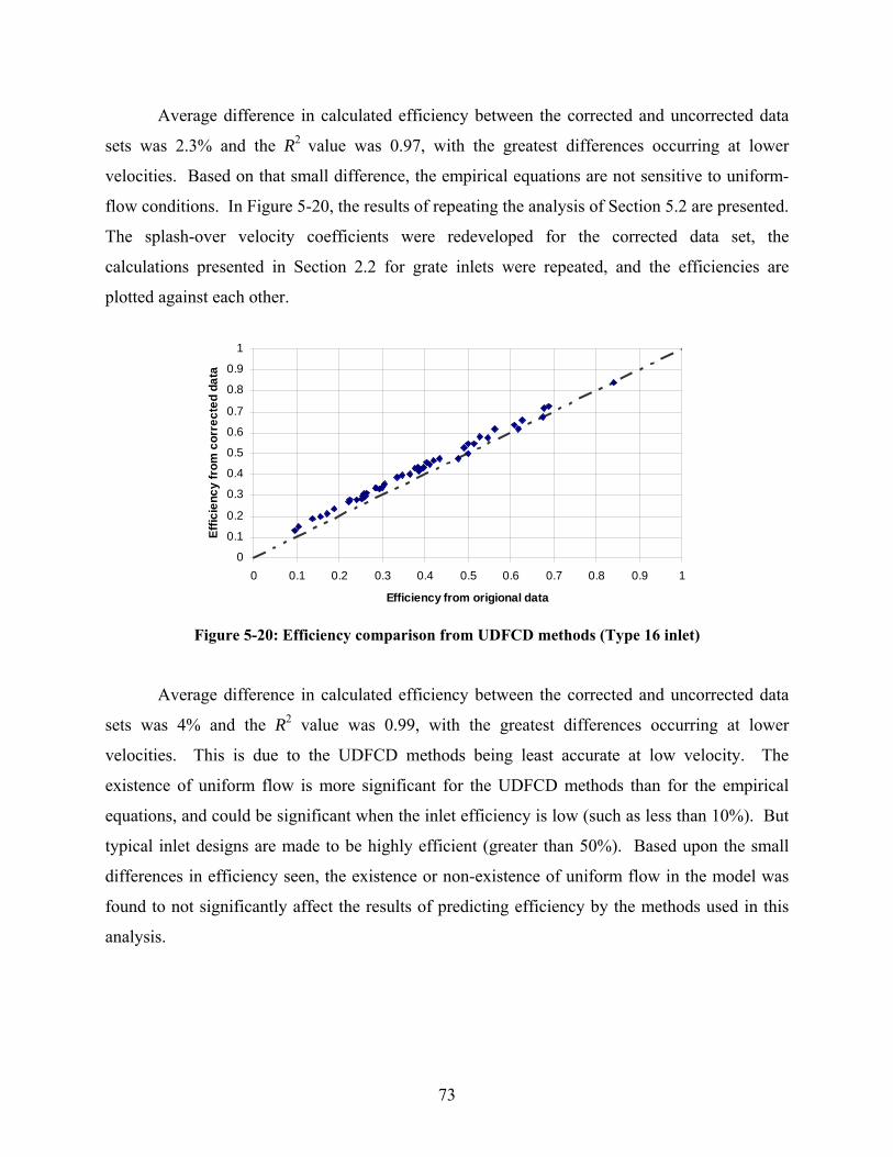
73
Average difference in calculated efficiency between the corrected and uncorrected data
sets was 2.3% and the R2 value was 0.97, with the greatest differences occurring at lower
velocities. Based on that small difference, the empirical equations are not sensitive to uniform-
flow conditions. In Figure 5-20, the results of repeating the analysis of Section 5.2 are presented.
The splash-over velocity coefficients were redeveloped for the corrected data set, the
calculations presented in Section 2.2 for grate inlets were repeated, and the efficiencies are
plotted against each other.
0
0.1
0.2
0.3
0.4
0.5
0.6
0.7
0.8
0.9
1
0 0.1 0.2 0.3 0.4 0.5 0.6 0.7 0.8 0.9 1
Efficiency from origional data
Effic
ienc
y fr
om c
orre
cted
dat
a
Figure 5-20: Efficiency comparison from UDFCD methods (Type 16 inlet)
Average difference in calculated efficiency between the corrected and uncorrected data
sets was 4% and the R2 value was 0.99, with the greatest differences occurring at lower
velocities. This is due to the UDFCD methods being least accurate at low velocity. The
existence of uniform flow is more significant for the UDFCD methods than for the empirical
equations, and could be significant when the inlet efficiency is low (such as less than 10%). But
typical inlet designs are made to be highly efficient (greater than 50%). Based upon the small
differences in efficiency seen, the existence or non-existence of uniform flow in the model was
found to not significantly affect the results of predicting efficiency by the methods used in this
analysis.
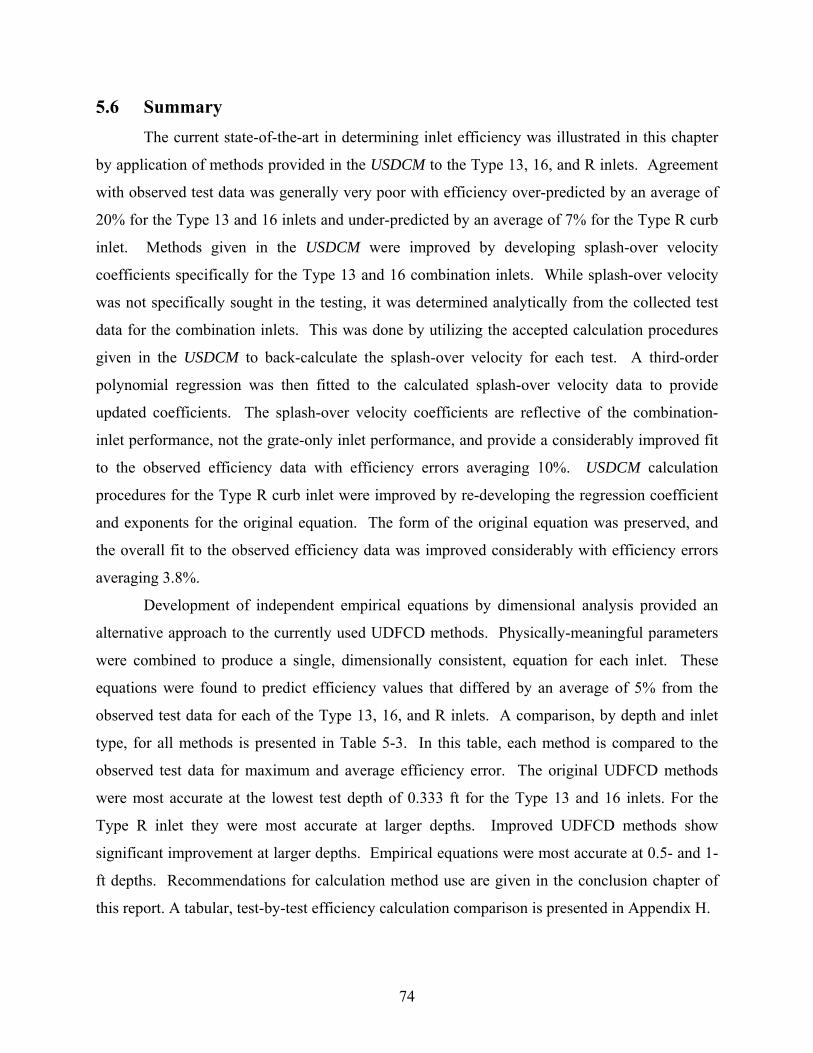
74
5.6 Summary The current state-of-the-art in determining inlet efficiency was illustrated in this chapter
by application of methods provided in the USDCM to the Type 13, 16, and R inlets. Agreement
with observed test data was generally very poor with efficiency over-predicted by an average of
20% for the Type 13 and 16 inlets and under-predicted by an average of 7% for the Type R curb
inlet. Methods given in the USDCM were improved by developing splash-over velocity
coefficients specifically for the Type 13 and 16 combination inlets. While splash-over velocity
was not specifically sought in the testing, it was determined analytically from the collected test
data for the combination inlets. This was done by utilizing the accepted calculation procedures
given in the USDCM to back-calculate the splash-over velocity for each test. A third-order
polynomial regression was then fitted to the calculated splash-over velocity data to provide
updated coefficients. The splash-over velocity coefficients are reflective of the combination-
inlet performance, not the grate-only inlet performance, and provide a considerably improved fit
to the observed efficiency data with efficiency errors averaging 10%. USDCM calculation
procedures for the Type R curb inlet were improved by re-developing the regression coefficient
and exponents for the original equation. The form of the original equation was preserved, and
the overall fit to the observed efficiency data was improved considerably with efficiency errors
averaging 3.8%.
Development of independent empirical equations by dimensional analysis provided an
alternative approach to the currently used UDFCD methods. Physically-meaningful parameters
were combined to produce a single, dimensionally consistent, equation for each inlet. These
equations were found to predict efficiency values that differed by an average of 5% from the
observed test data for each of the Type 13, 16, and R inlets. A comparison, by depth and inlet
type, for all methods is presented in Table 5-3. In this table, each method is compared to the
observed test data for maximum and average efficiency error. The original UDFCD methods
were most accurate at the lowest test depth of 0.333 ft for the Type 13 and 16 inlets. For the
Type R inlet they were most accurate at larger depths. Improved UDFCD methods show
significant improvement at larger depths. Empirical equations were most accurate at 0.5- and 1-
ft depths. Recommendations for calculation method use are given in the conclusion chapter of
this report. A tabular, test-by-test efficiency calculation comparison is presented in Appendix H.
75
Table 5-3: Efficiency error by depth and inlet type
Average Efficiency Error (%) Maximum Efficiency Error (%) Depth
(ft) UDFCD
UDFCD New
Empirical
Depth
(ft) UDFCD
UDFCD New
Empirical
Type 16 Type 16
0.333 10.8 9.7 10.3 0.333 28.1 28.1 21.9 0.5 19.9 11.6 2.8 0.5 39.0 37.7 9.2 1 22.3 6.0 2.3 1 35.4 23.4 5.5
Type 13 Type 13 0.333 8.9 7.2 8.6 0.333 22.2 22.2 15.5
0.5 22.4 12.2 2.9 0.5 32.3 31.0 8.1 1 25.3 6.7 1.5 1 34.0 16.4 4.2
Type R Type R 0.333 11.6 6.5 10.0 0.333 30.2 15.7 29.1
0.5 5.8 4.1 4.0 0.5 13.0 11.9 17.9 1 2.1 0.9 1.2 1 4.6 3.7 3.8
An efficiency comparison was made between a combination inlet, a grate-only inlet, and
a curb-only inlet for single Type 13 and 16 configurations. An average difference of 3%
efficiency was observed when the combination and the grate-only inlets were compared, and an
average difference of 12% efficiency was observed when the combination and curb-only inlets
were compared. Lastly, the relevance of uniform flow in the model was examined by repeating
the analysis with the observed test data adjusted to conditions of uniform flow. An average
efficiency difference of approximately 3%, as calculated by all methods, was noted between
uniform and non-uniform flow conditions in the model. From this small difference, the existence
or non-existence of uniform flow in the model was found to not affect the analysis significantly.

76

77
6 CONCLUSIONS AND RECOMMENDATIONS
6.1 Conclusions The data collected in this study, and the analysis performed, provided considerable
insight into the performance of the Type 13, 16, and R inlets under varying hydraulic conditions.
Physically-meaningful test conditions, that are likely to be encountered in the field, were created
in the model to supply a more complete body of test data than was previously available. The on-
grade test data were analyzed and improved methods were developed for determining inlet
efficiency. These improvements included: extending the currently used UDFCD methods (from
HEC-22) to include the Type 13 and 16 combination inlets, modifying the currently used
UDFCD methods for the Type R curb inlet, and developing independent empirical equations for
each of the three inlet types. The original UDFCD methods and equations were preserved in the
analysis. Empirical equations presented were developed independently from the UDFCD
methods, are dimensionally consistent, and provide a simple approach for calculation of inlet
efficiency. Physically-meaningful parameters, which can be easily determined by a user, were
combined using dimensional analysis to produce an equation for each of the Type 13
combination, Type 16 combination, and Type R curb inlets to predict inlet efficiency.
6.2 Recommendations for Inlet Efficiency Calculation The following guidance is provided for interpretation and use of the design criteria
developed in this study. Current UDFCD methods do not allow for determination of the true
efficiency for a combination inlet, which should take into account both the grate and the curb
openings. Design of combination inlets is typically done by assuming the grate portion of the
inlet acts alone (UDFCD, 2008). Both the empirical equations and the improved UDFCD
calculations presented in this report take into account the full capacity of the grate and the curb
opening. When the improved UDFCD methods were compared to the empirical equations for
the Type 13 and 16 combination inlets, the empirical equations were better able to predict the
78
test data for typical design depths of 0.5 to 1 ft. A 5% reduction in average efficiency error was
noted, and a 10% reduction in maximum efficiency error was noted for all test depths over the
improved UDFCD methods. UDFCD methods for these inlets were shown to rely heavily on
theoretical parameters that can not be physically determined by a user; parameters are instead
determined from complex empirical relationships. A comparison between splash-over velocity
curves developed for the Type 13 and 16 combination inlets and those for the most similar grate
inlets from the USDCM revealed significant differences. The equations provided in the USDCM
give an unrealistically high splash-over velocity (on the order of 30 ft/s) for a 10-ft Type 13 or 16
combination inlet, which is in sharp contrast to the 4 ft/s determined from the test data. Original
and improved UDFCD methods were most accurate at the lowest flow depth of 0.333 ft. Beyond
that depth, the accuracy was very poor. This is likely due to the limitations of the FHWA model
used to collect data for development of the equations. For the Type R curb inlet, the improved
UDFCD methods were slightly better able to predict the observed efficiency data than the
empirical equation for all test depths. A 1.2% improvement in average efficiency error was
noted over the empirical equation, and a 15% reduction in maximum efficiency error was noted
for all test depths. Typical design depths are 0.5 ft and greater for selection and placement of
street inlets (UDFCD, 2008). With this in mind, recommendations for which calculation method
to use are given as follows: for the Type 13 and 16 combination inlets the empirical equations
are recommended, for the Type R curb inlet the improved UDFCD methods are recommended.
For illustration purposes, the observed test data on efficiency are plotted with the empirical
efficiency and the efficiency determined from the improved UDFCD methods in Figure 6-1
through Figure 6-3.

79
0
0.1
0.2
0.3
0.4
0.5
0.6
0.7
0.8
0.9
1
0 0.1 0.2 0.3 0.4 0.5 0.6 0.7 0.8 0.9 1
Predicted efficiency
Obs
erve
d ef
ficie
ncy
Match lineregressionUDFCD new
Figure 6-1: Type 13 combination-inlet efficiency from all improved methods
0
0.1
0.2
0.3
0.4
0.5
0.6
0.7
0.8
0.9
1
0 0.1 0.2 0.3 0.4 0.5 0.6 0.7 0.8 0.9 1
Predicted efficiency
Obs
erve
d ef
ficie
ncy
Match lineregression
UDFCD new
Figure 6-2: Type 16 combination-inlet efficiency from all improved methods
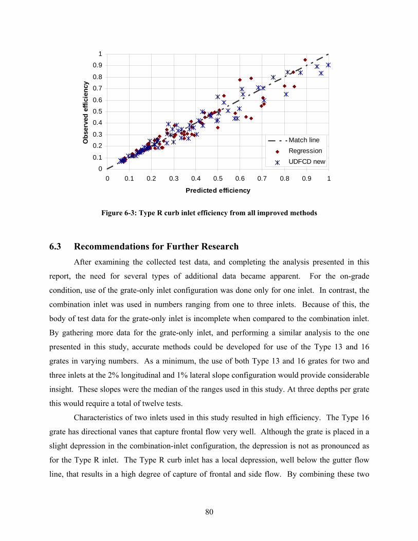
80
0
0.1
0.2
0.3
0.4
0.5
0.6
0.7
0.8
0.9
1
0 0.1 0.2 0.3 0.4 0.5 0.6 0.7 0.8 0.9 1
Predicted efficiency
Obs
erve
d ef
ficie
ncy
Match lineRegressionUDFCD new
Figure 6-3: Type R curb inlet efficiency from all improved methods
6.3 Recommendations for Further Research After examining the collected test data, and completing the analysis presented in this
report, the need for several types of additional data became apparent. For the on-grade
condition, use of the grate-only inlet configuration was done only for one inlet. In contrast, the
combination inlet was used in numbers ranging from one to three inlets. Because of this, the
body of test data for the grate-only inlet is incomplete when compared to the combination inlet.
By gathering more data for the grate-only inlet, and performing a similar analysis to the one
presented in this study, accurate methods could be developed for use of the Type 13 and 16
grates in varying numbers. As a minimum, the use of both Type 13 and 16 grates for two and
three inlets at the 2% longitudinal and 1% lateral slope configuration would provide considerable
insight. These slopes were the median of the ranges used in this study. At three depths per grate
this would require a total of twelve tests.
Characteristics of two inlets used in this study resulted in high efficiency. The Type 16
grate has directional vanes that capture frontal flow very well. Although the grate is placed in a
slight depression in the combination-inlet configuration, the depression is not as pronounced as
for the Type R inlet. The Type R curb inlet has a local depression, well below the gutter flow
line, that results in a high degree of capture of frontal and side flow. By combining these two
81
design characteristics, higher efficiency would result than either is capable of independently.
The local depression would act to reduce splash-over and capture more side flow, while the
directional vanes would capture frontal flow. A full testing program similar to this study would
be required to develop design equations, or extend the UDFCD methods, for such an inlet.
Engineering application of the Type 13 grate inlet typically involves placing a single grate in a
sump condition with no curb component (such as in a parking lot or field). Placing a single Type
13 grate in such a configuration typically exposes it to direct flow from all sides. In the testing
program performed for this study, the inlet was placed adjacent to a curb and exposed to lateral
flow from three sides. Only at the 1-ft flow depth was it exposed to flow from over the curb.
Testing the Type 13 grate in a true sump condition, where it is exposed to flow from all sides,
would provide additional useful data. A slightly different model than the one used in this study
would be necessary to collect data on this configuration.
For the analysis presented in this report, the observed test data were used in UDFCD
methods developed from the original FHWA model data. The purpose was to adapt the UDFCD
methods to include the inlets tested in this study. The converse of that analysis would be to use
the FHWA model data in the empirical equations developed in this report. A comparison could
then be made between the two methods and their ability to be adapted to suit other inlet types.
The additional testing suggested in this section would complete the body of knowledge
available for common application of the Type 13, 16, and R inlets. The UDFCD methods could
be easily extended to encompass the additional data, and independent design equations similar to
those presented in this study could be developed for the additional configurations.

82
83
7 REFERENCES
Bos, M. G. (1989). Discharge Measurement Structures. Third Edition revised, The Netherlands: Institute for Land Reclamation and Improvement.
Chaudhry, M. H. (2008). Open Channel Flow. Second Edition, New York, NY: Springer.
Federal Highway Administration (2001). Hydraulic Engineering Circular No. 22, Second Edition, Urban Drainage Design Manual. Publication FHWA-NHI-01-021, Springfield, VA: U. S. National Technical Information Service.
Federal Highway Administration (1977). Hydraulic and Safety Characteristics of Selected Grate Inlets on Continuous Grades, Vol 1. Publication FHWA-RD-77-24, Springfield, VA: U. S. National Technical Information Service.
Fox, R. W. (2006). Introduction to Fluid Mechanics. Sixth Edition, New York, NY: John Wiley and Sons, Inc.
Julien, P. Y. (2002). River Mechanics. New York, NY: Cambridge University Press.
Li, W. H. (1956). Design of Storm-Water Inlets. The Johns Hopkins University, Baltimore, MD.
U. S. Bureau of Reclamation (2001). Water Measurement Manual. Third Edition, U. S. Department of the Interior, Denver, CO.
Urban Drainage and Flood Control District (2008). Urban Storm Drainage Criteria Manual. Denver, CO.
Uyumaz, A. (2002). Urban Drainage with Curb Opening Inlets. In: Global Solutions for Urban Drainage, Proceedings of the Ninth International Conference on Urban Drainage, American Society of Civil Engineers.

84

85
APPENDIX A
USDCM GRATE INLET SCHEMATICS

86
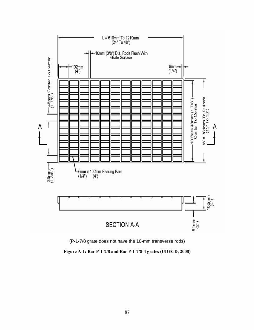
87
(P-1-7/8 grate does not have the 10-mm transverse rods)
Figure A-1: Bar P-1-7/8 and Bar P-1-7/8-4 grates (UDFCD, 2008)
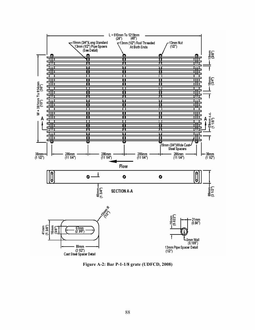
88
Figure A-2: Bar P-1-1/8 grate (UDFCD, 2008)
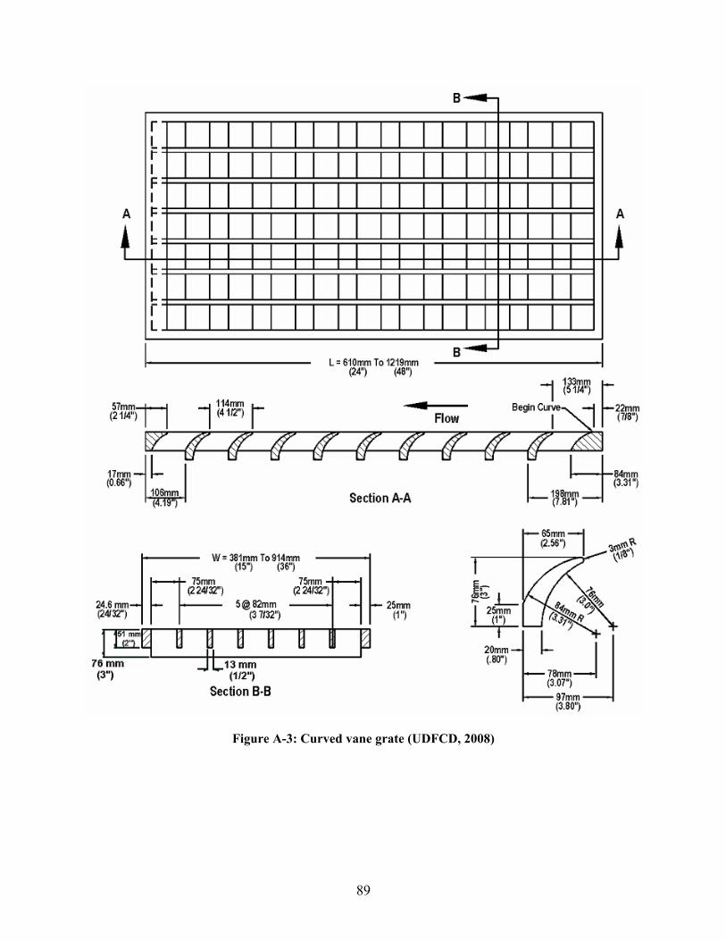
89
Figure A-3: Curved vane grate (UDFCD, 2008)

90
Figure A-4: 45º-tilt bar grate (UDFCD, 2008)

91
Figure A-5: 30º-tilt bar grate (UDFCD, 2008)
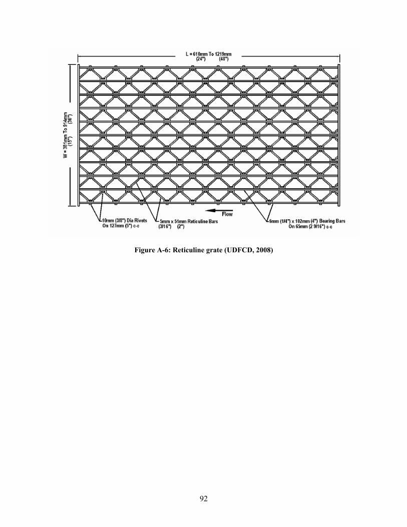
92
Figure A-6: Reticuline grate (UDFCD, 2008)

93
APPENDIX B
ON-GRADE TEST DATA

94

95
B.1 On-grade Test Results All three inlets (Types 13, 16, and R) were tested in the on-grade condition at various
slopes.
Table B-1: 0.5% and 1% on-grade test data
Test ID Number
Configuration
Longitudinal Slope
(%)
Cross Slope
(%)
Flow Depth
(ft)
Prototype Total Flow (cfs)
Efficiency (%)
Top Width at Control
(ft)
Top Width Down-stream
of Inlets (ft)
44 15-ft Type R (R15) 0.5 1 0.333 4.4 89.3 16.0 10.2 45 15-ft Type R (R15) 0.5 1 0.501 20.3 50.8 17.5 16.0 46 15-ft Type R (R15) 0.5 1 0.999 128.8 23.6 18.2 18.2 47 12-ft Type R (R12) 0.5 1 0.333 3.9 84.0 16.0 10.0 48 12-ft Type R (R12) 0.5 1 0.501 21.8 37.9 18.2 18.2 49 12-ft Type R (R12) 0.5 1 0.999 126.3 19.5 18.2 18.2 50 9-ft Type R (R9) 0.5 1 0.333 4.2 70.4 16.0 12.0 51 9-ft Type R (R9) 0.5 1 0.501 21.5 34.8 18.2 18.2 52 9-ft Type R (R9) 0.5 1 0.999 127.8 14.5 18.2 18.2 53 5-ft Type R (R5) 0.5 1 0.333 4.4 50.0 16.0 15.6 54 5-ft Type R (R5) 0.5 1 0.501 22.3 24.5 18.2 18.2 55 5-ft Type R (R5) 0.5 1 0.999 125.5 8.3 18.2 18.2 56 Triple No. 13 0.5 1 0.333 4.4 82.1 15.8 9.0 57 Triple No. 13 0.5 1 0.501 20.6 43.2 18.2 18.2 58 Triple No. 13 0.5 1 0.999 126.6 22.7 18.2 18.2 59 Double No. 13 0.5 1 0.333 4.7 73.3 16.0 10.7 60 Double No. 13 0.5 1 0.501 22.6 35.9 18.2 18.2 61 Double No. 13 0.5 1 0.999 127.8 16.2 18.2 18.2 62 Single No. 13 0.5 1 0.333 4.8 61.3 16.0 15.8 63 Single No. 13 0.5 1 0.501 26.2 23.8 18.2 18.2 64 Single No. 13 0.5 1 0.999 126.4 9.9 18.2 18.2 65 Single No. 16 0.5 1 0.333 5.1 60.6 16.0 15.8 66 Single No. 16 0.5 1 0.501 21.4 28.5 18.2 18.2 67 Single No. 16 0.5 1 0.999 126.9 13.5 18.2 18.2 68 Double No. 16 0.5 1 0.333 5.3 70.6 17.0 12.8 69 Double No. 16 0.5 1 0.501 23.2 34.2 18.2 18.2 70 Double No. 16 0.5 1 0.999 124.7 20.9 18.2 18.2 71 Triple No. 16 0.5 1 0.333 4.5 82.8 15.7 9.0 72 Triple No. 16 0.5 1 0.501 23.7 40.1 18.2 18.2 73 Triple No. 16 0.5 1 0.999 125.8 26.9 18.2 18.2
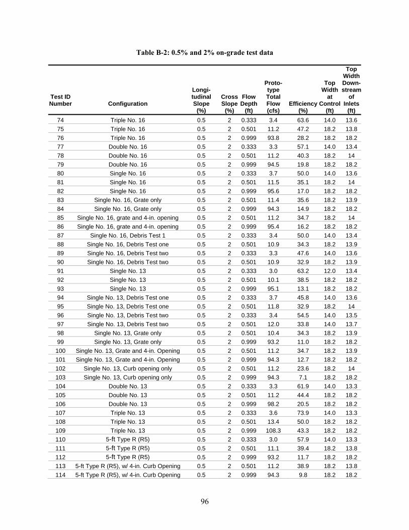
96
Table B-2: 0.5% and 2% on-grade test data
Test ID Number
Configuration
Longi-tudinal Slope
(%)
Cross Slope
(%)
Flow Depth
(ft)
Proto-type Total Flow (cfs)
Efficiency (%)
Top Width
at Control
(ft)
Top Width Down-stream
of Inlets
(ft) 74 Triple No. 16 0.5 2 0.333 3.4 63.6 14.0 13.6 75 Triple No. 16 0.5 2 0.501 11.2 47.2 18.2 13.8 76 Triple No. 16 0.5 2 0.999 93.8 28.2 18.2 18.2 77 Double No. 16 0.5 2 0.333 3.3 57.1 14.0 13.4 78 Double No. 16 0.5 2 0.501 11.2 40.3 18.2 14 79 Double No. 16 0.5 2 0.999 94.5 19.8 18.2 18.2 80 Single No. 16 0.5 2 0.333 3.7 50.0 14.0 13.6 81 Single No. 16 0.5 2 0.501 11.5 35.1 18.2 14 82 Single No. 16 0.5 2 0.999 95.6 17.0 18.2 18.2 83 Single No. 16, Grate only 0.5 2 0.501 11.4 35.6 18.2 13.9 84 Single No. 16, Grate only 0.5 2 0.999 94.3 14.9 18.2 18.2 85 Single No. 16, grate and 4-in. opening 0.5 2 0.501 11.2 34.7 18.2 14 86 Single No. 16, grate and 4-in. opening 0.5 2 0.999 95.4 16.2 18.2 18.2 87 Single No. 16, Debris Test 1 0.5 2 0.333 3.4 50.0 14.0 13.4 88 Single No. 16, Debris Test one 0.5 2 0.501 10.9 34.3 18.2 13.9 89 Single No. 16, Debris Test two 0.5 2 0.333 3.3 47.6 14.0 13.6 90 Single No. 16, Debris Test two 0.5 2 0.501 10.9 32.9 18.2 13.9 91 Single No. 13 0.5 2 0.333 3.0 63.2 12.0 13.4 92 Single No. 13 0.5 2 0.501 10.1 38.5 18.2 18.2 93 Single No. 13 0.5 2 0.999 95.1 13.1 18.2 18.2 94 Single No. 13, Debris Test one 0.5 2 0.333 3.7 45.8 14.0 13.6 95 Single No. 13, Debris Test one 0.5 2 0.501 11.8 32.9 18.2 14 96 Single No. 13, Debris Test two 0.5 2 0.333 3.4 54.5 14.0 13.5 97 Single No. 13, Debris Test two 0.5 2 0.501 12.0 33.8 14.0 13.7 98 Single No. 13, Grate only 0.5 2 0.501 10.4 34.3 18.2 13.9 99 Single No. 13, Grate only 0.5 2 0.999 93.2 11.0 18.2 18.2
100 Single No. 13, Grate and 4-in. Opening 0.5 2 0.501 11.2 34.7 18.2 13.9 101 Single No. 13, Grate and 4-in. Opening 0.5 2 0.999 94.3 12.7 18.2 18.2 102 Single No. 13, Curb opening only 0.5 2 0.501 11.2 23.6 18.2 14 103 Single No. 13, Curb opening only 0.5 2 0.999 94.3 7.1 18.2 18.2 104 Double No. 13 0.5 2 0.333 3.3 61.9 14.0 13.3 105 Double No. 13 0.5 2 0.501 11.2 44.4 18.2 18.2 106 Double No. 13 0.5 2 0.999 98.2 20.5 18.2 18.2 107 Triple No. 13 0.5 2 0.333 3.6 73.9 14.0 13.3 108 Triple No. 13 0.5 2 0.501 13.4 50.0 18.2 18.2 109 Triple No. 13 0.5 2 0.999 108.3 43.3 18.2 18.2 110 5-ft Type R (R5) 0.5 2 0.333 3.0 57.9 14.0 13.3 111 5-ft Type R (R5) 0.5 2 0.501 11.1 39.4 18.2 13.8 112 5-ft Type R (R5) 0.5 2 0.999 93.2 11.7 18.2 18.2 113 5-ft Type R (R5), w/ 4-in. Curb Opening 0.5 2 0.501 11.2 38.9 18.2 13.8 114 5-ft Type R (R5), w/ 4-in. Curb Opening 0.5 2 0.999 94.3 9.8 18.2 18.2
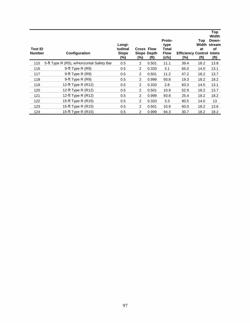
97
Test ID Number
Configuration
Longi-tudinal Slope
(%)
Cross Slope
(%)
Flow Depth
(ft)
Proto-type Total Flow (cfs)
Efficiency (%)
Top Width
at Control
(ft)
Top Width Down-stream
of Inlets
(ft) 115 5-ft Type R (R5), w/Horizontal Safety Bar 0.5 2 0.501 11.1 39.4 18.2 13.8 116 9-ft Type R (R9) 0.5 2 0.333 3.1 65.0 14.0 13.1 117 9-ft Type R (R9) 0.5 2 0.501 11.2 47.2 18.2 13.7 118 9-ft Type R (R9) 0.5 2 0.999 93.8 19.3 18.2 18.2 119 12-ft Type R (R12) 0.5 2 0.333 2.8 83.3 14.0 13.1 120 12-ft Type R (R12) 0.5 2 0.501 10.9 52.9 18.2 13.7 121 12-ft Type R (R12) 0.5 2 0.999 93.8 25.4 18.2 18.2 122 15-ft Type R (R15) 0.5 2 0.333 3.3 90.5 14.0 13 123 15-ft Type R (R15) 0.5 2 0.501 10.9 60.0 18.2 13.6 124 15-ft Type R (R15) 0.5 2 0.999 94.3 30.7 18.2 18.2
98
Table B-3: 2% and 1% on-grade test data
Test ID Number
Configuration
Longi- tudinal Slope
(%)
Cross Slope
(%)
Flow Depth
(ft)
Proto- type Total Flow (cfs)
Efficiency (%)
Top Width at Control
(ft)
Top Width Down-stream
of Inlets (ft)
125 15-ft Type R (R15) 2 1 0.333 14.8 44.2 18.2 16 126 15-ft Type R (R15) 2 1 0.501 33.5 30.2 18.2 18.2 127 15-ft Type R (R15) 2 1 0.999 178.5 17.6 18.2 18.2 128 12-ft Type R (R12) 2 1 0.333 13.4 43.0 18.2 16 129 12-ft Type R (R12) 2 1 0.501 32.9 27.0 18.2 18.2 130 12-ft Type R (R12) 2 1 0.999 176.1 14.7 18.2 18.2 131 9-ft Type R (R9) 2 1 0.333 13.4 36.0 18.2 16 132 9-ft Type R (R9) 2 1 0.501 29.6 22.6 18.2 18.2 133 9-ft Type R (R9) 2 1 0.999 173.0 11.4 18.2 18.2 134 5-ft Type R (R5) 2 1 0.333 13.1 25.0 18.2 16 135 5-ft Type R (R5) 2 1 0.501 28.4 16.5 18.2 18.2 136 5-ft Type R (R5) 2 1 0.999 179.0 7.6 18.2 18.2 137 Triple No. 16 2 1 0.333 13.2 44.7 18.2 16 138 Triple No. 16 2 1 0.501 39.9 30.9 18.2 18.2 139 Triple No. 16 2 1 0.999 155.1 23.6 18.2 18.2 140 Double No. 16 2 1 0.333 14.7 36.2 18.2 16 141 Double No. 16 2 1 0.501 32.7 27.1 18.2 18.2 142 Double No. 16 2 1 0.999 177.1 18.7 18.2 18.2 143 Single No. 16 2 1 0.333 15.3 28.6 18.2 16 144 Single No. 16 2 1 0.501 34.0 20.6 18.2 18.2 145 Single No. 16 2 1 0.999 176.6 12.3 18.2 18.2 146 Single No. 13 2 1 0.333 15.9 27.5 18.2 16 147 Single No. 13 2 1 0.501 33.7 20.4 18.2 18.2 148 Single No. 13 2 1 0.999 166.6 9.4 18.2 18.2 149 Double No. 13 2 1 0.333 14.3 33.7 18.2 16 150 Double No. 13 2 1 0.501 33.7 23.6 18.2 18.2 151 Double No. 13 2 1 0.999 176.6 13.3 18.2 18.2 152 Triple No. 13 2 1 0.333 13.1 42.9 18.2 16 153 Triple No. 13 2 1 0.501 31.0 28.6 18.2 18.2 154 Triple No. 13 2 1 0.999 177.7 17.7 18.2 18.2
99
Table B-4: 2% and 2% on-grade test data
Test ID Number
Configuration
Longi- tudinal Slope
(%)
Cross Slope
(%)
Flow Depth
(ft)
Proto-type Total Flow (cfs)
Efficiency (%)
Top Width
at Control
(ft)
Top Width Down-stream
of Inlets
(ft) 155 Triple No. 13 2 2 0.333 7.8 74.0 16.0 8.3 156 Triple No. 13 2 2 0.501 22.1 43.7 18.2 18.2 157 Triple No. 13 2 2 0.999 163.2 19.1 18.2 18.2 158 Double No. 13 2 2 0.333 8.1 63.5 16.0 8.3 159 Double No. 13 2 2 0.501 23.4 34.7 18.2 18.2 160 Double No. 13 2 2 0.999 161.3 14.3 18.2 18.2 161 Single No. 13 2 2 0.333 7.8 50.0 14.8 9 162 Single No. 13 2 2 0.501 24.8 23.9 18.2 18.2 163 Single No. 13 2 2 0.999 155.9 8.9 18.2 18.2 164 Single No. 13, Debris Test one 2 2 0.333 7.3 40.4 14.0 8.3 165 Single No. 13, Debris Test one 2 2 0.501 24.0 17.5 18.2 18.2 166 Single No. 13, Debris Test two 2 2 0.333 7.2 47.8 14.0 8.3 167 Single No. 13, Debris Test two 2 2 0.501 24.0 19.5 18.2 18.2 168 Single No. 13, Grate Only 2 2 0.501 23.2 19.5 18.2 18.2 169 Single No. 13, Grate Only 2 2 0.999 154.3 6.6 18.2 18.2 170 Single No. 13, Grate and 4-in. Opening 2 2 0.501 22.3 25.2 18.2 15.8 171 Single No. 13, Grate and 4-in. Opening 2 2 0.999 164.1 8.2 18.2 18.2 172 Single No. 13, Curb opening only 2 2 0.501 24.2 9.7 18.2 18.2 173 Single No. 13, Curb opening only 2 2 0.999 155.9 3.7 18.2 18.2 174 Single No. 16 2 2 0.333 7.9 54.9 14.0 8.6 175 Single No. 16 2 2 0.501 22.3 31.5 18.2 15.6 176 Single No. 16 2 2 0.999 162.9 12.6 18.2 18.2 177 Single No. 16, Grate only 2 2 0.501 22.9 27.2 18.2 15.7 178 Single No. 16, Grate only 2 2 0.999 162.9 10.3 18.2 18.2 179 Single No. 16, Grate and 4-in. Opening 2 2 0.501 22.3 28.7 18.2 18.2 180 Single No. 16, Grate and 4-in. Opening 2 2 0.999 164.1 11.5 18.2 18.2 181 Single No. 16, Debris Test one 2 2 0.333 8.1 53.8 14.0 8.9 182 Single No. 16, Debris Test one 2 2 0.501 24.0 27.3 18.2 18.2 183 Single No. 16, Debris Test two 2 2 0.333 8.4 51.9 14.0 8.9 184 Single No. 16, Debris Test two 2 2 0.501 24.9 25.6 18.2 18.2 185 Double No. 16 2 2 0.333 7.9 64.7 14.0 8.3 186 Double No. 16 2 2 0.501 23.7 36.8 18.2 18.2 187 Double No. 16 2 2 0.999 163.7 20.3 18.2 18.2 188 Triple No. 16 2 2 0.333 8.4 72.2 14.0 8.3 189 Triple No. 16 2 2 0.501 22.6 46.2 18.2 18.2 190 Triple No. 16 2 2 0.999 162.9 25.7 18.2 18.2 191 5-ft Type R (R5) 2 2 0.333 7.3 38.3 17.8 11.3 192 5-ft Type R (R5) 2 2 0.501 22.9 18.4 18.2 18.2 193 5-ft Type R (R5) 2 2 0.999 166.0 7.1 18.2 18.2 194 5-ft Type R (R5), w/ 4-in. Curb Opening 2 2 0.999 166.8 5.4 18.2 18.2 195 5-ft Type R (R5), w/ 4-in. Curb Opening 2 2 0.501 22.8 18.5 18.2 18.2

100
Test ID Number
Configuration
Longi- tudinal Slope
(%)
Cross Slope
(%)
Flow Depth
(ft)
Proto-type Total Flow (cfs)
Efficiency (%)
Top Width
at Control
(ft)
Top Width Down-stream
of Inlets
(ft) 196 5-ft Type R (R5), w/ Horizontal Safety Bar 2 2 0.501 23.1 18.2 18.2 18.2 197 9-ft Type R (R9) 2 2 0.333 6.2 65.0 11.0 6.8 198 9-ft Type R (R9) 2 2 0.501 21.8 33.6 18.2 14.3 199 9-ft Type R (R9) 2 2 0.999 166.0 11.6 18.2 18.2 200 12-ft Type R (R12) 2 2 0.333 7.5 70.8 14.0 9.8 201 12-ft Type R (R12) 2 2 0.501 21.7 42.4 18.2 15.8 202 12-ft Type R (R12) 2 2 0.999 166.8 15.2 18.2 18.2 203 15-ft Type R (R15) 2 2 0.333 7.0 84.4 14.0 8.3 204 15-ft Type R (R15) 2 2 0.501 21.5 48.6 18.2 15.8 205 15-ft Type R (R15) 2 2 0.999 166.8 18.8 18.2 18.2
101
Table B-5: 4% and 1% on-grade test data
Test ID Number
Configuration
Longi- tudinal Slope
(%)
Cross Slope
(%)
Flow Depth
(ft)
Proto- type Total Flow (cfs)
Efficiency (%)
Top Width at Control
(ft)
Top Width Down-stream
of Inlets (ft)
206 15-ft Type R (R15) 4 1 0.333 13.1 44.0 18.2 16 207 15-ft Type R (R15) 4 1 0.501 38.3 26.8 18.2 18.2 208 15-ft Type R (R15) 4 1 0.999 143.4 18.6 18.2 18.2 209 12-ft Type R (R12) 4 1 0.333 12.6 42.0 18.2 16 210 12-ft Type R (R12) 4 1 0.501 38.3 23.6 18.2 18.2 211 12-ft Type R (R12) 4 1 0.999 152.9 14.9 18.2 18.2 212 9-ft Type R (R9) 4 1 0.333 13.9 34.8 18.2 16 213 9-ft Type R (R9) 4 1 0.501 38.2 18.8 18.2 18.2 214 9-ft Type R (R9) 4 1 0.999 141.5 11.7 18.2 18.2 215 5-ft Type R (R5) 4 1 0.333 13.7 21.6 18.2 16 216 5-ft Type R (R5) 4 1 0.501 38.2 11.4 18.2 18.2 217 5-ft Type R (R5) 4 1 0.999 140.3 6.9 18.2 18.2 218 Triple No. 16 4 1 0.333 12.6 42.0 18.2 16 219 Triple No. 16 4 1 0.501 38.2 29.4 18.2 18.2 220 Triple No. 16 4 1 0.999 145.7 24.8 18.2 18.2 221 Double No. 16 4 1 0.333 13.2 37.6 18.2 16 222 Double No. 16 4 1 0.501 36.6 25.1 18.2 18.2 223 Double No. 16 4 1 0.999 145.0 20.4 18.2 18.2 224 Single No. 16 4 1 0.333 13.1 33.3 18.2 16 225 Single No. 16 4 1 0.501 37.9 20.2 18.2 18.2 226 Single No. 16 4 1 0.999 141.2 14.0 18.2 18.2 227 Single No. 13 4 1 0.333 12.9 25.3 18.2 16 228 Single No. 13 4 1 0.501 37.7 12.8 18.2 18.2 229 Single No. 13 4 1 0.999 142.6 8.4 18.2 18.2 230 Double No. 13 4 1 0.333 13.2 37.6 18.2 16 231 Double No. 13 4 1 0.501 36.6 21.3 18.2 18.2 232 Double No. 13 4 1 0.999 138.7 13.5 18.2 18.2 233 Triple No. 13 4 1 0.333 12.6 40.7 18.2 16 234 Triple No. 13 4 1 0.501 38.2 24.9 18.2 18.2 235 Triple No. 13 4 1 0.999 146.8 17.9 18.2 18.2
102
Table B-6: 4% and 2% on-grade test data
Test ID Number
Configuration
Longi-tudinal Slope
(%)
Cross Slope
(%)
Flow Depth
(ft)
Proto- type Total Flow (cfs)
Efficiency (%)
Top Width
at Control
(ft)
Top Width Down-stream
of Inlets
(ft) 236 Triple No. 13 4 2 0.333 8.4 74.1 15.5 7.7 237 Triple No. 13 4 2 0.501 25.7 42.4 18.2 14.3 238 Triple No. 13 4 2 0.999 128.6 20.5 18.2 18.2 239 Double No. 13 4 2 0.333 8.3 66.0 15.5 7.8 240 Double No. 13 4 2 0.501 26.0 32.9 18.2 14.3 241 Double No. 13 4 2 0.999 127.8 15.9 18.2 18.2 242 Single No. 13 4 2 0.333 9.0 43.1 15.5 7.7 243 Single No. 13 4 2 0.501 27.3 20.6 18.2 13.7 244 Single No. 13 4 2 0.999 129.7 9.5 18.2 18.2 245 Single No. 13, Debris Test one 4 2 0.333 8.6 34.5 16.0 8.6 246 Single No. 13, Debris Test one 4 2 0.501 26.5 15.9 17.5 14.3 247 Single No. 13, Debris Test two 4 2 0.333 8.4 40.7 16.0 8 248 Single No. 13, Debris Test two 4 2 0.501 27.1 16.7 18.2 14.3 249 Single No. 13, Curb opening only 4 2 0.501 26.5 9.4 18.2 14.3 250 Single No. 13, Curb opening only 4 2 0.999 119.2 4.7 18.2 18.2 251 Single No. 13, Grate Only 4 2 0.501 21.8 19.3 18.2 9.8 252 Single No. 13, Grate Only 4 2 0.999 117.7 6.5 18.2 18.2 253 Single No. 13, Grate and 4-in. Opening 4 2 0.501 24.5 21.7 18.2 14.3 254 Single No. 13, Grate and 4-in. Opening 4 2 0.999 113.3 9.9 18.2 18.2 255 Single No. 16, Grate and 4-in. Opening 4 2 0.501 28.2 31.5 18.2 14.3 256 Single No. 16, Grate and 4-in. Opening 4 2 0.999 123.1 15.3 18.2 18.2 257 Single No. 16, Grate only 4 2 0.501 30.4 28.7 18.2 12.8 258 Single No. 16, Grate only 4 2 0.999 133.4 12.7 18.2 18.2 259 Single No. 16, Debris Test one 4 2 0.333 8.1 55.8 18.2 7.4 260 Single No. 16, Debris Test one 4 2 0.501 26.5 25.9 18.2 14.3 261 Single No. 16, Debris Test two 4 2 0.333 8.1 48.1 18.2 8 262 Single No. 16, Debris Test two 4 2 0.501 26.8 17.4 18.2 14.3 263 Single No. 16 4 2 0.333 7.5 64.6 14.6 7.8 264 Single No. 16 4 2 0.501 28.1 31.7 18.2 14.3 265 Single No. 16 4 2 0.999 129.4 15.7 18.2 18.2 266 Double No. 16 4 2 0.333 8.7 67.9 14.6 7.8 267 Double No. 16 4 2 0.501 26.5 37.6 18.2 14.3 268 Double No. 16 4 2 0.999 130.9 24.6 18.2 18.2 269 Triple No. 16 4 2 0.333 8.4 74.1 14.6 7.7 270 Triple No. 16 4 2 0.501 25.7 43.6 18.2 14.3 271 Triple No. 16 4 2 0.999 127.8 29.0 18.2 18.2 272 5-ft Type R (R5) 4 2 0.333 8.1 34.6 16.0 8.6 273 5-ft Type R (R5) 4 2 0.501 26.7 17.0 18.2 14.3 274 5-ft Type R (R5) 4 2 0.999 118.9 7.9 18.2 18.2 275 5-ft Type R (R5), w/ 4-in. Curb Opening 4 2 0.501 27.4 16.5 18.2 14.3 276 5-ft Type R (R5), w/ 4-in. Curb Opening 4 2 0.999 128.6 6.2 18.2 18.2
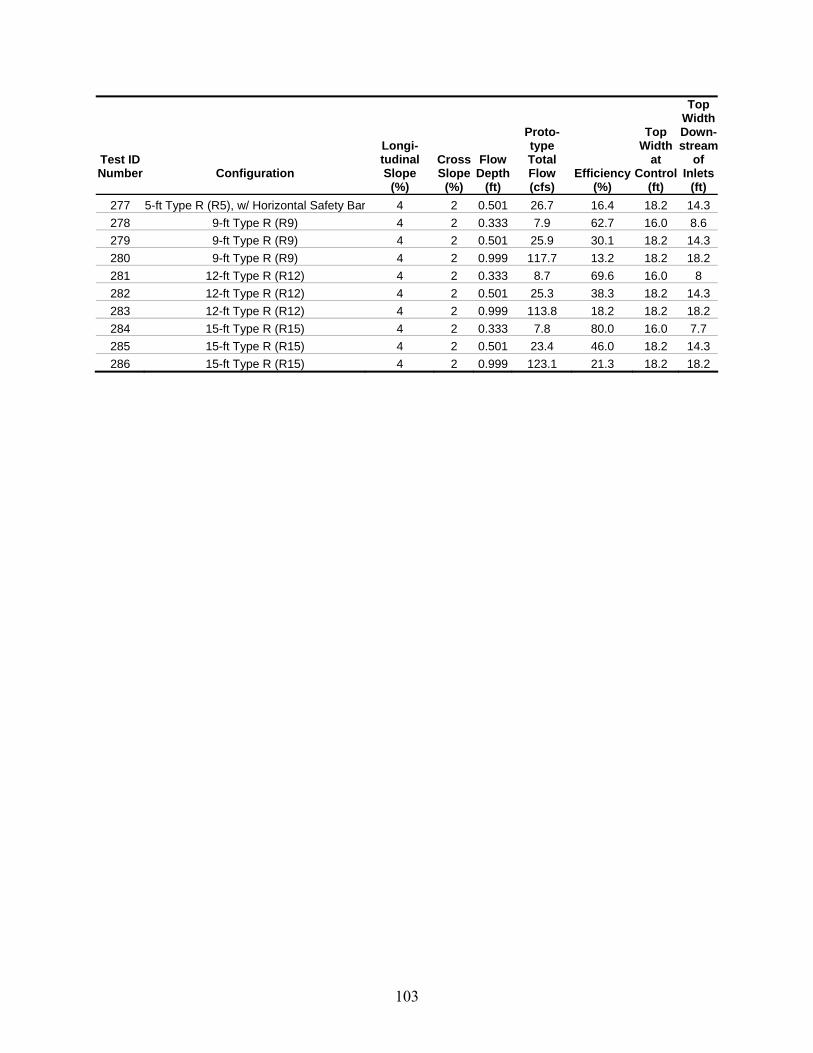
103
Test ID Number
Configuration
Longi-tudinal Slope
(%)
Cross Slope
(%)
Flow Depth
(ft)
Proto- type Total Flow (cfs)
Efficiency (%)
Top Width
at Control
(ft)
Top Width Down-stream
of Inlets
(ft) 277 5-ft Type R (R5), w/ Horizontal Safety Bar 4 2 0.501 26.7 16.4 18.2 14.3 278 9-ft Type R (R9) 4 2 0.333 7.9 62.7 16.0 8.6 279 9-ft Type R (R9) 4 2 0.501 25.9 30.1 18.2 14.3 280 9-ft Type R (R9) 4 2 0.999 117.7 13.2 18.2 18.2 281 12-ft Type R (R12) 4 2 0.333 8.7 69.6 16.0 8 282 12-ft Type R (R12) 4 2 0.501 25.3 38.3 18.2 14.3 283 12-ft Type R (R12) 4 2 0.999 113.8 18.2 18.2 18.2 284 15-ft Type R (R15) 4 2 0.333 7.8 80.0 16.0 7.7 285 15-ft Type R (R15) 4 2 0.501 23.4 46.0 18.2 14.3 286 15-ft Type R (R15) 4 2 0.999 123.1 21.3 18.2 18.2
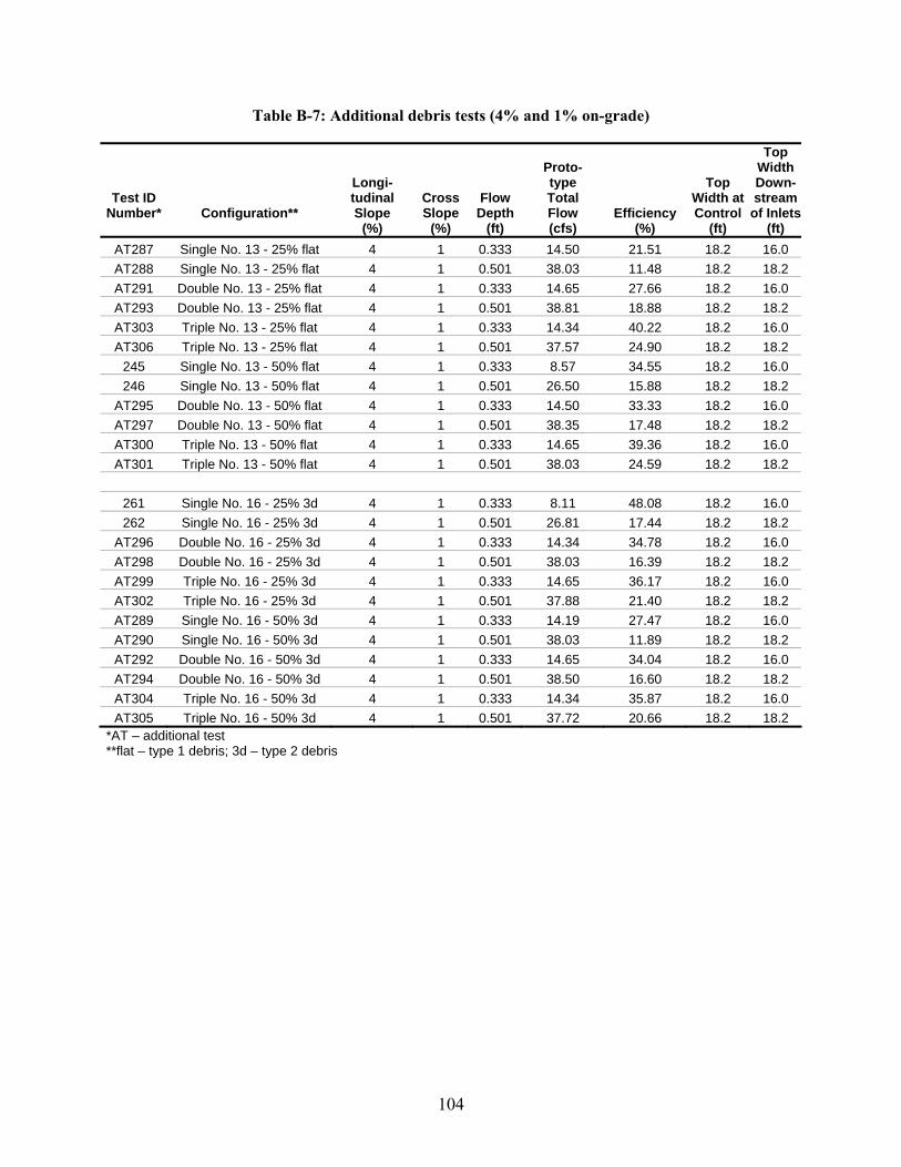
104
Table B-7: Additional debris tests (4% and 1% on-grade)
Test ID Number*
Configuration**
Longi-tudinal Slope
(%)
Cross Slope
(%)
Flow Depth
(ft)
Proto- type Total Flow (cfs)
Efficiency (%)
Top Width at Control
(ft)
Top Width Down-stream
of Inlets (ft)
AT287 Single No. 13 - 25% flat 4 1 0.333 14.50 21.51 18.2 16.0 AT288 Single No. 13 - 25% flat 4 1 0.501 38.03 11.48 18.2 18.2 AT291 Double No. 13 - 25% flat 4 1 0.333 14.65 27.66 18.2 16.0 AT293 Double No. 13 - 25% flat 4 1 0.501 38.81 18.88 18.2 18.2 AT303 Triple No. 13 - 25% flat 4 1 0.333 14.34 40.22 18.2 16.0 AT306 Triple No. 13 - 25% flat 4 1 0.501 37.57 24.90 18.2 18.2
245 Single No. 13 - 50% flat 4 1 0.333 8.57 34.55 18.2 16.0 246 Single No. 13 - 50% flat 4 1 0.501 26.50 15.88 18.2 18.2
AT295 Double No. 13 - 50% flat 4 1 0.333 14.50 33.33 18.2 16.0 AT297 Double No. 13 - 50% flat 4 1 0.501 38.35 17.48 18.2 18.2 AT300 Triple No. 13 - 50% flat 4 1 0.333 14.65 39.36 18.2 16.0 AT301 Triple No. 13 - 50% flat 4 1 0.501 38.03 24.59 18.2 18.2
261 Single No. 16 - 25% 3d 4 1 0.333 8.11 48.08 18.2 16.0 262 Single No. 16 - 25% 3d 4 1 0.501 26.81 17.44 18.2 18.2
AT296 Double No. 16 - 25% 3d 4 1 0.333 14.34 34.78 18.2 16.0 AT298 Double No. 16 - 25% 3d 4 1 0.501 38.03 16.39 18.2 18.2 AT299 Triple No. 16 - 25% 3d 4 1 0.333 14.65 36.17 18.2 16.0 AT302 Triple No. 16 - 25% 3d 4 1 0.501 37.88 21.40 18.2 18.2 AT289 Single No. 16 - 50% 3d 4 1 0.333 14.19 27.47 18.2 16.0 AT290 Single No. 16 - 50% 3d 4 1 0.501 38.03 11.89 18.2 18.2 AT292 Double No. 16 - 50% 3d 4 1 0.333 14.65 34.04 18.2 16.0 AT294 Double No. 16 - 50% 3d 4 1 0.501 38.50 16.60 18.2 18.2 AT304 Triple No. 16 - 50% 3d 4 1 0.333 14.34 35.87 18.2 16.0 AT305 Triple No. 16 - 50% 3d 4 1 0.501 37.72 20.66 18.2 18.2
*AT – additional test **flat – type 1 debris; 3d – type 2 debris

105
APPENDIX C
SUMP TEST DATA

106

107
C.1 Sump Test Data All three inlets (Types 13, 16, and R) were tested in the sump condition.
Table C-1: Sump test data
Test ID Number
Configuration
Longitudinal Slope
(%)
Cross Slope
(%)
Flow Depth
(ft)
Prototype Flow (cfs)
1 Triple No. 13 0 1 0.333 2.5 2 Triple No. 13 0 1 0.501 8.6 3 Triple No. 13 0 1 0.999 42.2 4 Double No. 13 0 1 0.333 2.3 5 Double No. 13 0 1 0.501 7.8 6 Double No. 13 0 1 0.999 27.1 7 Single No. 13 0 1 0.333 2.0 8 Single No. 13 0 1 0.501 5.9 9 Single No. 13 0 1 0.999 15.3 10 Single No. 13, Curb opening only 0 1 0.501 5.1 11 Single No. 13, Curb opening only 0 1 0.999 6.1 12 Single No. 13, Grate only 0 1 0.501 10.3 13 Single No. 13, Grate only 0 1 0.999 11.4 14 Single No. 13, w/ 4-in. opening 0 1 0.501 5.8 15 Single No. 13, w/ 4-in. opening 0 1 0.999 15.1 16 Single No. 16, Grate only 0 1 0.501 3.6 17 Single No. 16, Grate only 0 1 0.999 13.7 18 Single No. 16, w/ 4-in. opening 0 1 0.501 5.5 19 Single No. 16, w/ 4-in. opening 0 1 0.999 7.5 20 Single No. 16 0 1 0.333 2.3 21 Single No. 16 0 1 0.501 6.2 22 Single No. 16 0 1 0.999 13.9 23 Double No. 16 0 1 0.333 2.5 24 Double No. 16 0 1 0.501 7.6 25 Double No. 16 0 1 0.999 26.5 26 Triple No. 16 0 1 0.333 2.8 27 Triple No. 16 0 1 0.501 8.4 28 Triple No. 16 0 1 0.999 37.4 29 5-ft Type R (R5) 0 1 0.333 2.2 30 5-ft Type R (R5) 0 1 0.501 7.3 31 5-ft Type R (R5) 0 1 0.999 12.6 32 5-ft Type R (R5), w/ 4-in. Curb Opening 0 1 0.501 6.4 33 5-ft Type R (R5), w/ 4-in. Curb Opening 0 1 0.999 8.9 34 5-ft Type R (R5), Horizontal Safety Bar 0 1 0.501 7.3 35 9-ft Type R (R9) 0 1 0.333 2.5 36 9-ft Type R (R9) 0 1 0.501 8.7 37 9-ft Type R (R9) 0 1 0.999 24.2 38 12-ft Type R (R12) 0 1 0.333 2.8 39 12-ft Type R (R12) 0 1 0.501 10.0 40 12-ft Type R (R12) 0 1 0.999 32.9 41 15-ft Type R (R15) 0 1 0.333 2.8 42 15-ft Type R (R15) 0 1 0.501 10.1 43 15-ft Type R (R15) 0 1 0.999 42.1
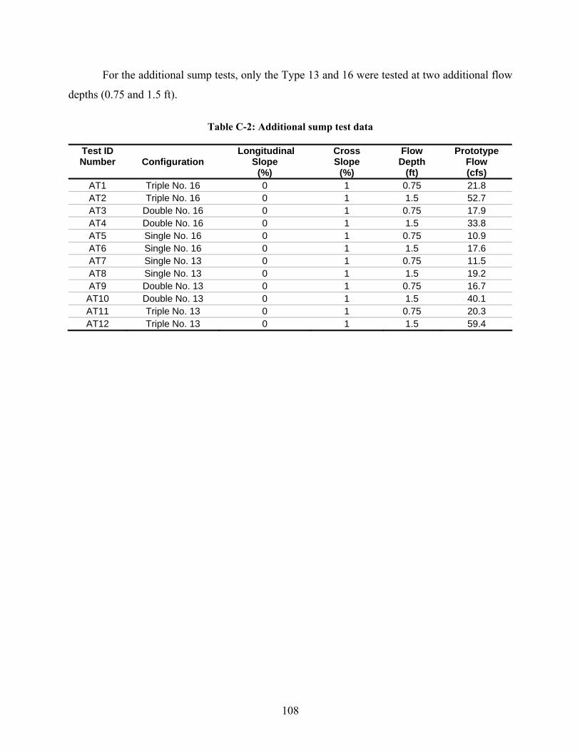
108
For the additional sump tests, only the Type 13 and 16 were tested at two additional flow
depths (0.75 and 1.5 ft).
Table C-2: Additional sump test data
Test ID Number
Configuration
Longitudinal Slope
(%)
Cross Slope
(%)
Flow Depth
(ft)
Prototype Flow (cfs)
AT1 Triple No. 16 0 1 0.75 21.8 AT2 Triple No. 16 0 1 1.5 52.7 AT3 Double No. 16 0 1 0.75 17.9 AT4 Double No. 16 0 1 1.5 33.8 AT5 Single No. 16 0 1 0.75 10.9 AT6 Single No. 16 0 1 1.5 17.6 AT7 Single No. 13 0 1 0.75 11.5 AT8 Single No. 13 0 1 1.5 19.2 AT9 Double No. 13 0 1 0.75 16.7 AT10 Double No. 13 0 1 1.5 40.1 AT11 Triple No. 13 0 1 0.75 20.3 AT12 Triple No. 13 0 1 1.5 59.4

109
APPENDIX D
INLET CONSTRUCTION DRAWINGS

110

111
D.1 Inlet Drawings
(a) (b)
Figure D-1: Type 13 inlet specifications

112
(a)
(b)
Figure D-2: Type 16 inlet specifications
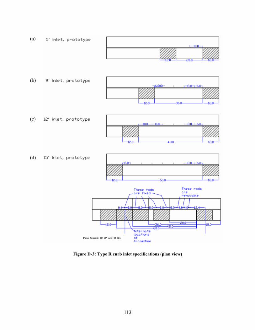
113
(a)
(b)
(c)
(d)
Figure D-3: Type R curb inlet specifications (plan view)

114
(a)
(b)
(c)
Figure D-4: Type R curb inlet specifications (profile view)

115
APPENDIX E
DATA COLLECTION

116

117
UDFCD Curb and Grate Study Data Sheet
Date: Test ID Number: Operators (first initial and last name): Start Time: End Time: Water Temperature (ºF): Model Information Cross Slope: 1% 2% Longitudinal Slope: 0% 0.5% 2% 4% Model Configuration (circle one): Denver Type 13 Denver Type 16 Type R Inlet Configuration (circle one): Single Double Triple 5-ft 9-ft 12-ft 15-ft Debris: Y N 4-ft curb opening: Y N Other:
Discharge Information Venturi Reading (cfs): Mag Meter Reading (cfs): Annubar (cfs): Through Grates (ft of head): Bypassing Grates (ft of head):
Flow Characteristics Extent of Flow (station and distance from river right wall): See Back of Sheet Depth of Flow, at 5 ft Upstream, Model: Gutter Flow Line Depth:
Verbal Description of Flow into Inlets Note: Upstream grate is #1, second is #2, and the furthest downstream is # 3. Approximate distribution of flow through inlets:
(Over)
UDFCD Sheet (Page 1 of 2)

118
Extent of Flow
Station (x) Position (y) Notes
Notes and Observations:
UDFCD Sheet (Page 2 of 2)

119
APPENDIX F
ADDITIONAL PARAMETERS

120
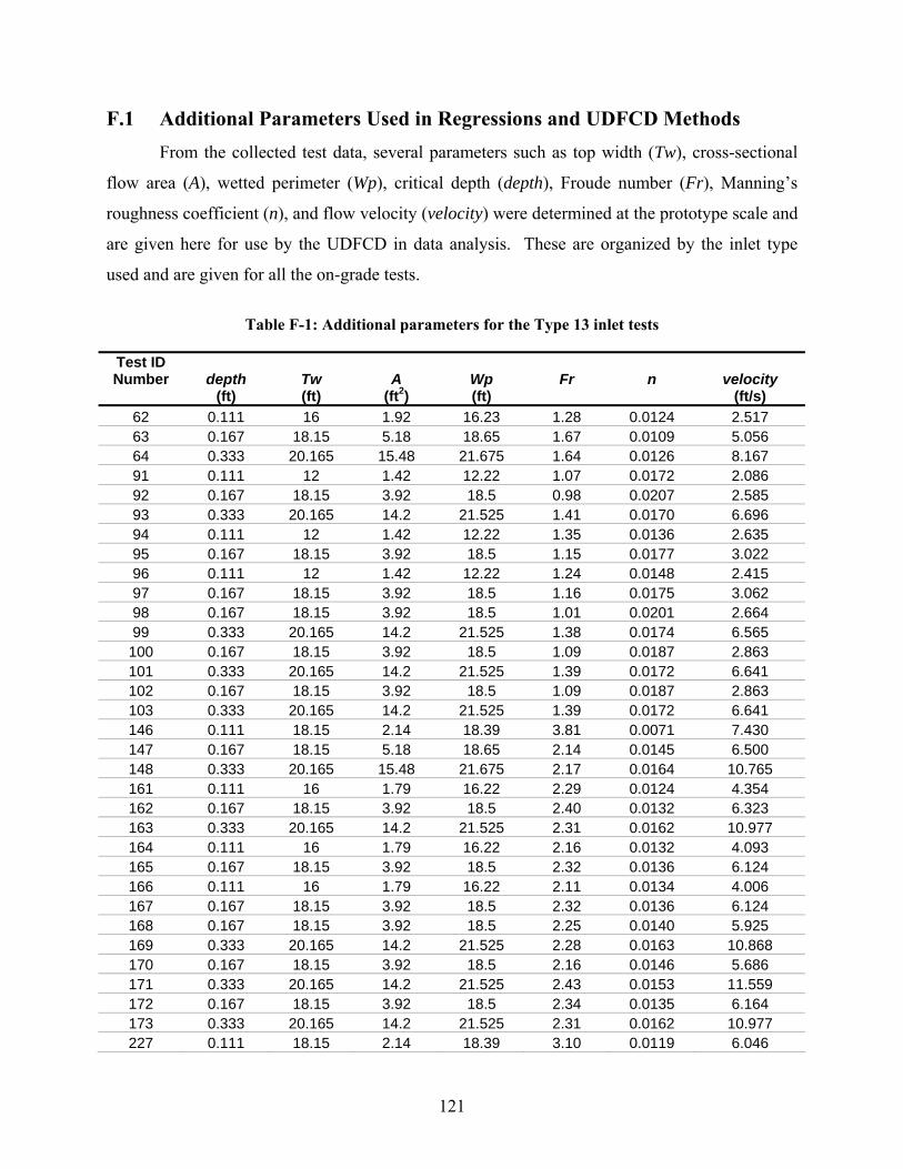
121
F.1 Additional Parameters Used in Regressions and UDFCD Methods From the collected test data, several parameters such as top width (Tw), cross-sectional
flow area (A), wetted perimeter (Wp), critical depth (depth), Froude number (Fr), Manning’s
roughness coefficient (n), and flow velocity (velocity) were determined at the prototype scale and
are given here for use by the UDFCD in data analysis. These are organized by the inlet type
used and are given for all the on-grade tests.
Table F-1: Additional parameters for the Type 13 inlet tests
Test ID Number
depth
(ft) Tw (ft)
A (ft2)
Wp (ft)
Fr
n
velocity (ft/s)
62 0.111 16 1.92 16.23 1.28 0.0124 2.517 63 0.167 18.15 5.18 18.65 1.67 0.0109 5.056 64 0.333 20.165 15.48 21.675 1.64 0.0126 8.167 91 0.111 12 1.42 12.22 1.07 0.0172 2.086 92 0.167 18.15 3.92 18.5 0.98 0.0207 2.585 93 0.333 20.165 14.2 21.525 1.41 0.0170 6.696 94 0.111 12 1.42 12.22 1.35 0.0136 2.635 95 0.167 18.15 3.92 18.5 1.15 0.0177 3.022 96 0.111 12 1.42 12.22 1.24 0.0148 2.415 97 0.167 18.15 3.92 18.5 1.16 0.0175 3.062 98 0.167 18.15 3.92 18.5 1.01 0.0201 2.664 99 0.333 20.165 14.2 21.525 1.38 0.0174 6.565 100 0.167 18.15 3.92 18.5 1.09 0.0187 2.863 101 0.333 20.165 14.2 21.525 1.39 0.0172 6.641 102 0.167 18.15 3.92 18.5 1.09 0.0187 2.863 103 0.333 20.165 14.2 21.525 1.39 0.0172 6.641 146 0.111 18.15 2.14 18.39 3.81 0.0071 7.430 147 0.167 18.15 5.18 18.65 2.14 0.0145 6.500 148 0.333 20.165 15.48 21.675 2.17 0.0164 10.765 161 0.111 16 1.79 16.22 2.29 0.0124 4.354 162 0.167 18.15 3.92 18.5 2.40 0.0132 6.323 163 0.333 20.165 14.2 21.525 2.31 0.0162 10.977 164 0.111 16 1.79 16.22 2.16 0.0132 4.093 165 0.167 18.15 3.92 18.5 2.32 0.0136 6.124 166 0.111 16 1.79 16.22 2.11 0.0134 4.006 167 0.167 18.15 3.92 18.5 2.32 0.0136 6.124 168 0.167 18.15 3.92 18.5 2.25 0.0140 5.925 169 0.333 20.165 14.2 21.525 2.28 0.0163 10.868 170 0.167 18.15 3.92 18.5 2.16 0.0146 5.686 171 0.333 20.165 14.2 21.525 2.43 0.0153 11.559 172 0.167 18.15 3.92 18.5 2.34 0.0135 6.164 173 0.333 20.165 14.2 21.525 2.31 0.0162 10.977 227 0.111 18.15 2.14 18.39 3.10 0.0119 6.046
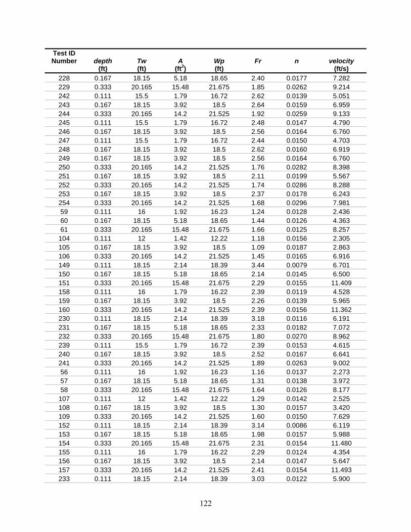
122
Test ID Number
depth
(ft) Tw (ft)
A (ft2)
Wp (ft)
Fr
n
velocity (ft/s)
228 0.167 18.15 5.18 18.65 2.40 0.0177 7.282 229 0.333 20.165 15.48 21.675 1.85 0.0262 9.214 242 0.111 15.5 1.79 16.72 2.62 0.0139 5.051 243 0.167 18.15 3.92 18.5 2.64 0.0159 6.959 244 0.333 20.165 14.2 21.525 1.92 0.0259 9.133 245 0.111 15.5 1.79 16.72 2.48 0.0147 4.790 246 0.167 18.15 3.92 18.5 2.56 0.0164 6.760 247 0.111 15.5 1.79 16.72 2.44 0.0150 4.703 248 0.167 18.15 3.92 18.5 2.62 0.0160 6.919 249 0.167 18.15 3.92 18.5 2.56 0.0164 6.760 250 0.333 20.165 14.2 21.525 1.76 0.0282 8.398 251 0.167 18.15 3.92 18.5 2.11 0.0199 5.567 252 0.333 20.165 14.2 21.525 1.74 0.0286 8.288 253 0.167 18.15 3.92 18.5 2.37 0.0178 6.243 254 0.333 20.165 14.2 21.525 1.68 0.0296 7.981 59 0.111 16 1.92 16.23 1.24 0.0128 2.436 60 0.167 18.15 5.18 18.65 1.44 0.0126 4.363 61 0.333 20.165 15.48 21.675 1.66 0.0125 8.257 104 0.111 12 1.42 12.22 1.18 0.0156 2.305 105 0.167 18.15 3.92 18.5 1.09 0.0187 2.863 106 0.333 20.165 14.2 21.525 1.45 0.0165 6.916 149 0.111 18.15 2.14 18.39 3.44 0.0079 6.701 150 0.167 18.15 5.18 18.65 2.14 0.0145 6.500 151 0.333 20.165 15.48 21.675 2.29 0.0155 11.409 158 0.111 16 1.79 16.22 2.39 0.0119 4.528 159 0.167 18.15 3.92 18.5 2.26 0.0139 5.965 160 0.333 20.165 14.2 21.525 2.39 0.0156 11.362 230 0.111 18.15 2.14 18.39 3.18 0.0116 6.191 231 0.167 18.15 5.18 18.65 2.33 0.0182 7.072 232 0.333 20.165 15.48 21.675 1.80 0.0270 8.962 239 0.111 15.5 1.79 16.72 2.39 0.0153 4.615 240 0.167 18.15 3.92 18.5 2.52 0.0167 6.641 241 0.333 20.165 14.2 21.525 1.89 0.0263 9.002 56 0.111 16 1.92 16.23 1.16 0.0137 2.273 57 0.167 18.15 5.18 18.65 1.31 0.0138 3.972 58 0.333 20.165 15.48 21.675 1.64 0.0126 8.177 107 0.111 12 1.42 12.22 1.29 0.0142 2.525 108 0.167 18.15 3.92 18.5 1.30 0.0157 3.420 109 0.333 20.165 14.2 21.525 1.60 0.0150 7.629 152 0.111 18.15 2.14 18.39 3.14 0.0086 6.119 153 0.167 18.15 5.18 18.65 1.98 0.0157 5.988 154 0.333 20.165 15.48 21.675 2.31 0.0154 11.480 155 0.111 16 1.79 16.22 2.29 0.0124 4.354 156 0.167 18.15 3.92 18.5 2.14 0.0147 5.647 157 0.333 20.165 14.2 21.525 2.41 0.0154 11.493 233 0.111 18.15 2.14 18.39 3.03 0.0122 5.900

123
Test ID Number
depth
(ft) Tw (ft)
A (ft2)
Wp (ft)
Fr
n
velocity (ft/s)
234 0.167 18.15 5.18 18.65 2.43 0.0175 7.373 235 0.333 20.165 15.48 21.675 1.91 0.0255 9.486 236 0.111 15.5 1.79 16.72 2.44 0.0150 4.703 237 0.167 18.15 3.92 18.5 2.49 0.0169 6.561 238 0.333 20.165 14.2 21.525 1.90 0.0261 9.056
AT287 0.111 18.15 2.14 18.39 3.48 0.0106 6.774 AT288 0.167 18.15 5.18 18.65 2.42 0.0175 7.343 AT291 0.111 18.15 2.14 18.39 3.51 0.0105 6.847 AT293 0.167 18.15 5.18 18.65 2.47 0.0172 7.493 AT303 0.111 18.15 2.14 18.39 3.44 0.0108 6.701 AT306 0.167 18.15 5.18 18.65 2.39 0.0178 7.252 AT295 0.111 18.15 2.14 18.39 3.48 0.0106 6.774 AT297 0.167 18.15 5.18 18.65 2.44 0.0174 7.403 AT300 0.111 18.15 2.14 18.39 3.51 0.0105 6.847 AT301 0.167 18.15 5.18 18.65 2.42 0.0175 7.343

124
Table F-2: Additional parameters for the Type 16 inlet tests
Test ID Number
depth
(ft) Tw (ft)
A (ft2)
Wp (ft)
Fr
n
velocity (ft/s)
65 0.111 17 1.88 17.22 1.45 0.0108 2.736 66 0.167 18.15 5.18 18.65 1.36 0.0133 4.123 67 0.333 20.165 15.48 21.675 1.65 0.0126 8.197 80 0.111 12 1.42 12.22 1.35 0.0136 2.635 81 0.167 18.15 3.92 18.5 1.12 0.0182 2.943 82 0.333 20.165 14.2 21.525 1.41 0.0170 6.729 83 0.167 18.15 3.92 18.5 1.10 0.0184 2.903 84 0.333 20.165 14.2 21.525 1.39 0.0172 6.641 85 0.167 18.15 3.92 18.5 1.09 0.0187 2.863 86 0.333 20.165 14.2 21.525 1.41 0.0170 6.718 87 0.111 12 1.42 12.22 1.24 0.0148 2.415 88 0.167 18.15 3.92 18.5 1.06 0.0192 2.784 89 0.111 12 1.42 12.22 1.18 0.0156 2.305 90 0.167 18.15 3.92 18.5 1.06 0.0192 2.784 143 0.111 18.15 2.14 18.39 3.66 0.0074 7.138 144 0.167 18.15 5.18 18.65 2.16 0.0143 6.560 145 0.333 20.165 15.48 21.675 2.29 0.0155 11.409 174 0.111 14 1.6 14.22 2.59 0.0110 4.969 175 0.167 18.15 3.92 18.5 2.16 0.0146 5.686 176 0.333 20.165 14.2 21.525 2.41 0.0155 11.471 177 0.167 18.15 3.92 18.5 2.22 0.0142 5.846 178 0.333 20.165 14.2 21.525 2.41 0.0155 11.471 179 0.167 18.15 3.92 18.5 2.16 0.0146 5.686 180 0.333 20.165 14.2 21.525 2.43 0.0153 11.559 181 0.111 14 1.6 14.22 2.64 0.0108 5.066 182 0.167 18.15 3.92 18.5 2.32 0.0136 6.124 183 0.111 14 1.6 14.22 2.74 0.0104 5.261 184 0.167 18.15 3.92 18.5 2.41 0.0131 6.362 224 0.111 18.15 2.14 18.39 3.14 0.0118 6.119 225 0.167 18.15 5.18 18.65 2.41 0.0176 7.313 226 0.333 20.165 15.48 21.675 1.83 0.0265 9.123 255 0.167 18.15 3.92 18.5 2.73 0.0149 7.198 256 0.333 20.165 14.2 21.525 1.82 0.0264 8.672 257 0.167 18.15 3.92 18.5 2.94 0.0139 7.754 258 0.333 20.165 14.2 21.525 1.97 0.0244 9.397 259 0.111 14.6 1.66 14.82 2.55 0.0144 4.883 260 0.167 18.15 3.92 18.5 2.56 0.0159 6.760 261 0.111 14.6 1.66 14.82 2.55 0.0144 4.883 262 0.167 18.15 3.92 18.5 2.59 0.0157 6.840 263 0.111 14.6 1.66 14.82 2.36 0.0161 4.507 264 0.167 18.15 3.92 18.5 2.71 0.0155 7.158 265 0.333 20.165 14.2 21.525 1.91 0.0260 9.111 68 0.111 17 1.88 17.22 1.49 0.0105 2.819 69 0.167 18.15 5.18 18.65 1.48 0.0123 4.484

125
Test ID Number
depth
(ft) Tw (ft)
A (ft2)
Wp (ft)
Fr
n
velocity (ft/s)
70 0.333 20.165 15.48 21.675 1.62 0.0128 8.056 77 0.111 12 1.42 12.22 1.18 0.0156 2.305 78 0.167 18.15 3.92 18.5 1.09 0.0187 2.863 79 0.333 20.165 14.2 21.525 1.40 0.0172 6.652 140 0.111 18.15 2.14 18.39 3.51 0.0077 6.847 141 0.167 18.15 5.18 18.65 2.08 0.0149 6.319 142 0.333 20.165 15.48 21.675 2.30 0.0154 11.439 185 0.111 14 1.6 14.22 2.59 0.0110 4.969 186 0.167 18.15 3.92 18.5 2.29 0.0138 6.044 187 0.333 20.165 14.2 21.525 2.42 0.0154 11.526 221 0.111 18.15 2.14 18.39 3.18 0.0116 6.191 222 0.167 18.15 5.18 18.65 2.33 0.0182 7.072 223 0.333 20.165 15.48 21.675 1.88 0.0258 9.365 266 0.111 14.6 1.66 14.82 2.75 0.0138 5.259 267 0.167 18.15 3.92 18.5 2.56 0.0164 6.760 268 0.333 20.165 14.2 21.525 1.94 0.0257 9.221 71 0.111 17 1.88 17.22 1.27 0.0123 2.405 72 0.167 18.15 5.18 18.65 1.51 0.0120 4.574 73 0.333 20.165 15.48 21.675 1.63 0.0127 8.126 74 0.111 12 1.42 12.22 1.24 0.0148 2.415 75 0.167 18.15 3.92 18.5 1.09 0.0187 2.863 76 0.333 20.165 14.2 21.525 1.39 0.0173 6.608 137 0.111 18.15 2.14 18.39 3.18 0.0085 6.191 138 0.167 18.15 5.18 18.65 2.54 0.0122 7.704 139 0.333 20.165 15.48 21.675 2.02 0.0176 10.019 188 0.111 14 1.6 14.22 2.74 0.0104 5.261 189 0.167 18.15 3.92 18.5 2.19 0.0144 5.766 190 0.333 20.165 14.2 21.525 2.41 0.0155 11.471 218 0.111 18.15 2.14 18.39 3.03 0.0122 5.900 219 0.167 18.15 5.18 18.65 2.43 0.0175 7.373 220 0.333 20.165 15.48 21.675 1.89 0.0257 9.415 269 0.111 14.6 1.66 14.82 2.65 0.0143 5.071 270 0.167 18.15 3.92 18.5 2.49 0.0169 6.561 271 0.333 20.165 14.2 21.525 1.89 0.0263 9.002
AT296 0.111 18.15 2.14 18.39 3.44 0.0108 6.701 AT298 0.167 18.15 5.18 18.65 2.42 0.0175 7.343 AT299 0.111 18.15 2.14 18.39 3.51 0.0105 6.847 AT302 0.167 18.15 5.18 18.65 2.41 0.0176 7.313 AT289 0.111 18.15 2.14 18.39 3.40 0.0109 6.629 AT290 0.167 18.15 5.18 18.65 2.42 0.0175 7.343 AT292 0.111 18.15 2.14 18.39 3.51 0.0105 6.847 AT294 0.167 18.15 5.18 18.65 2.45 0.0173 7.433 AT304 0.111 18.15 2.14 18.39 3.44 0.0108 6.701 AT305 0.167 18.15 5.18 18.65 2.40 0.0177 7.282 AT303 0.111 18.15 2.14 18.39 3.44 0.0108 6.701 AT306 0.167 18.15 5.18 18.65 2.39 0.0178 7.252
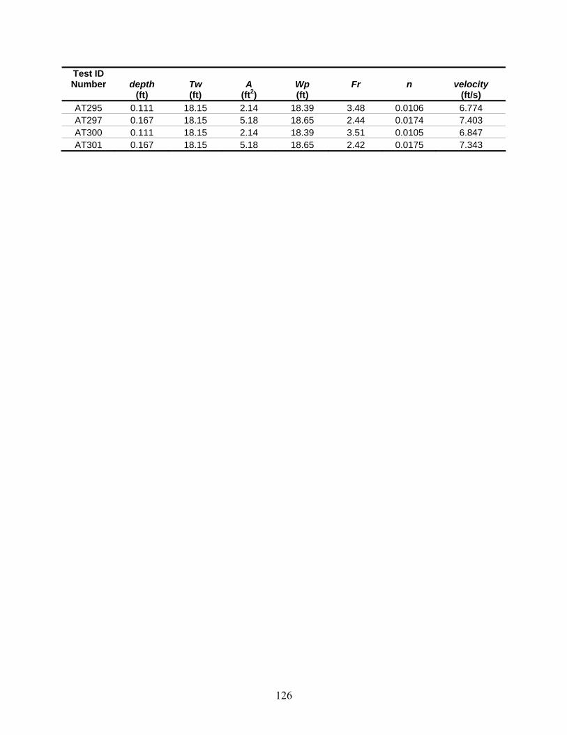
126
Test ID Number
depth
(ft) Tw (ft)
A (ft2)
Wp (ft)
Fr
n
velocity (ft/s)
AT295 0.111 18.15 2.14 18.39 3.48 0.0106 6.774 AT297 0.167 18.15 5.18 18.65 2.44 0.0174 7.403 AT300 0.111 18.15 2.14 18.39 3.51 0.0105 6.847 AT301 0.167 18.15 5.18 18.65 2.42 0.0175 7.343

127
Table F-3: Additional parameters for the Type R curb inlet tests
Test ID Number
depth
(ft) Tw (ft)
A (ft2)
Wp (ft)
Fr
n
velocity (ft/s)
44 0.111 16.000 1.92 1.809 1.16 0.0137 2.273 45 0.167 17.500 4.96 4.793 1.35 0.0139 4.086 46 0.333 20.165 15.48 15.147 1.67 0.0124 8.318 47 0.111 16.000 1.92 1.809 1.03 0.0153 2.030 48 0.167 18.150 5.18 5.013 1.39 0.0131 4.213 49 0.333 20.165 15.48 15.147 1.64 0.0127 8.157 50 0.111 16.000 1.92 1.809 1.12 0.0142 2.192 51 0.167 18.150 5.18 5.013 1.37 0.0132 4.153 52 0.333 20.165 15.48 15.147 1.66 0.0125 8.257 53 0.111 16.000 1.92 1.809 1.16 0.0137 2.273 54 0.167 18.150 5.18 5.013 1.42 0.0128 4.303 55 0.333 20.165 15.48 15.147 1.63 0.0127 8.106 122 0.111 14.000 1.6 1.489 1.07 0.0172 2.046 123 0.167 18.150 3.92 3.753 1.06 0.0192 2.784 124 0.333 20.165 14.2 13.867 1.39 0.0172 6.641 119 0.111 14.000 1.6 1.489 0.91 0.0200 1.754 120 0.167 18.150 3.92 3.753 1.06 0.0192 2.784 121 0.333 20.165 14.2 13.867 1.39 0.0173 6.608 116 0.111 14.000 1.6 1.489 1.02 0.0180 1.949 117 0.167 18.150 3.92 3.753 1.09 0.0187 2.863 118 0.333 20.165 14.2 13.867 1.39 0.0173 6.608 110 0.111 14.000 1.6 1.489 0.96 0.0190 1.851 111 0.167 18.150 3.92 3.753 1.07 0.0190 2.823 112 0.333 20.165 14.2 13.867 1.38 0.0174 6.565 113 0.167 18.150 3.92 3.753 1.09 0.0187 2.863 114 0.333 20.165 14.2 13.867 1.39 0.0172 6.641 115 0.167 18.150 3.92 3.753 1.07 0.0190 2.823 125 0.111 18.150 2.14 2.029 3.55 0.0076 6.920 126 0.167 18.150 5.18 5.013 2.13 0.0145 6.470 127 0.333 20.165 15.48 15.147 2.32 0.0153 11.530 128 0.111 18.150 2.14 2.029 3.21 0.0084 6.264 129 0.167 18.150 5.18 5.013 2.09 0.0148 6.350 130 0.333 20.165 15.48 15.147 2.29 0.0155 11.379 131 0.111 18.150 2.14 2.029 3.21 0.0084 6.264 132 0.167 18.150 5.18 5.013 1.89 0.0164 5.718 133 0.333 20.165 15.48 15.147 2.25 0.0158 11.177 134 0.111 18.150 2.14 2.029 3.14 0.0086 6.119 135 0.167 18.150 5.18 5.013 1.81 0.0172 5.477 136 0.333 20.165 15.48 15.147 2.33 0.0153 11.560 203 0.111 14.000 1.6 1.489 2.29 0.0124 4.384 204 0.167 18.150 3.92 3.753 2.08 0.0152 5.488 205 0.333 20.165 14.2 13.867 2.47 0.0151 11.746 200 0.111 14.000 1.6 1.489 2.44 0.0117 4.676 201 0.167 18.150 3.92 3.753 2.10 0.0150 5.527

128
Test ID Number
depth
(ft) Tw (ft)
A (ft2)
Wp (ft)
Fr
n
velocity (ft/s)
202 0.333 20.165 14.2 13.867 2.47 0.0151 11.746 197 0.111 11.000 1.34 1.229 2.35 0.0122 4.653 198 0.167 18.150 3.92 3.753 2.11 0.0149 5.567 199 0.333 20.165 14.2 13.867 2.46 0.0152 11.691 191 0.111 17.800 1.95 1.839 2.00 0.0141 3.757 192 0.167 18.150 3.92 3.753 2.22 0.0142 5.846 193 0.333 20.165 14.2 13.867 2.46 0.0152 11.691 194 0.333 20.165 14.2 13.867 2.47 0.0151 11.746 195 0.167 18.150 3.92 3.753 2.20 0.0143 5.806 196 0.167 18.150 3.92 3.753 2.23 0.0141 5.885 206 0.111 18.150 2.14 2.029 3.14 0.0118 6.119 207 0.167 18.150 5.18 5.013 2.44 0.0174 7.403 208 0.333 20.165 15.48 15.147 1.86 0.0261 9.264 209 0.111 18.150 2.14 2.029 3.03 0.0122 5.900 210 0.167 18.150 5.18 5.013 2.44 0.0174 7.403 211 0.333 20.165 15.48 15.147 1.99 0.0245 9.878 212 0.111 18.150 2.14 2.029 3.33 0.0111 6.483 213 0.167 18.150 5.18 5.013 2.43 0.0175 7.373 214 0.333 20.165 15.48 15.147 1.84 0.0264 9.143 215 0.111 18.150 2.14 2.029 3.29 0.0112 6.410 216 0.167 18.150 5.18 5.013 2.43 0.0175 7.373 217 0.333 20.165 15.48 15.147 1.82 0.0267 9.063 284 0.111 16.000 1.79 1.679 2.29 0.0165 4.354 285 0.167 18.150 3.92 3.753 2.26 0.0186 5.965 286 0.333 20.165 14.2 13.867 1.82 0.0273 8.672 281 0.111 16.000 1.79 1.679 2.57 0.0147 4.877 282 0.167 18.150 3.92 3.753 2.44 0.0172 6.442 283 0.333 20.165 14.2 13.867 1.68 0.0295 8.014 278 0.111 16.000 1.79 1.679 2.34 0.0162 4.441 279 0.167 18.150 3.92 3.753 2.50 0.0168 6.601 280 0.333 20.165 14.2 13.867 1.74 0.0286 8.288 272 0.111 16.000 1.79 1.679 2.39 0.0159 4.528 273 0.167 18.150 3.92 3.753 2.58 0.0163 6.800 274 0.333 20.165 14.2 13.867 1.76 0.0283 8.376 275 0.167 18.15 3.92 3.753 2.65 0.0159 6.999 276 0.333 20.165 14.2 13.867 1.90 0.0261 9.056 277 0.167 18.15 3.92 3.753 2.58 0.0163 6.800
AT302 0.167 18.15 5.18 18.65 2.41 0.0176 7.313 AT289 0.111 18.15 2.14 18.39 3.40 0.0109 6.629 AT290 0.167 18.15 5.18 18.65 2.42 0.0175 7.343 AT292 0.111 18.15 2.14 18.39 3.51 0.0105 6.847 AT294 0.167 18.15 5.18 18.65 2.45 0.0173 7.433 AT304 0.111 18.15 2.14 18.39 3.44 0.0108 6.701 AT305 0.167 18.15 5.18 18.65 2.40 0.0177 7.282 AT303 0.111 18.15 2.14 18.39 3.44 0.0108 6.701 AT306 0.167 18.15 5.18 18.65 2.39 0.0178 7.252

129
Test ID Number
depth
(ft) Tw (ft)
A (ft2)
Wp (ft)
Fr
n
velocity (ft/s)
AT295 0.111 18.15 2.14 18.39 3.48 0.0106 6.774 AT297 0.167 18.15 5.18 18.65 2.44 0.0174 7.403 AT300 0.111 18.15 2.14 18.39 3.51 0.0105 6.847 AT301 0.167 18.15 5.18 18.65 2.42 0.0175 7.343

130

131
APPENDIX G
REGRESSION ANALYSIS STATISTICS

132
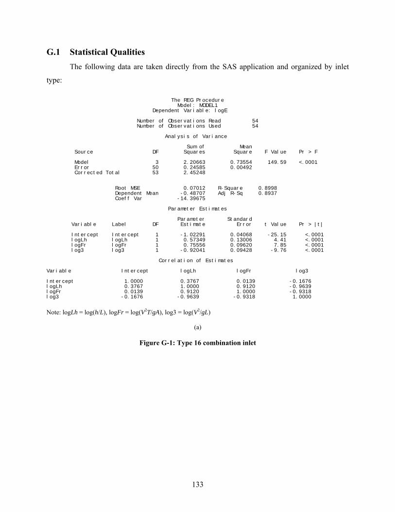
133
G.1 Statistical Qualities The following data are taken directly from the SAS application and organized by inlet
type:
The REG Procedure Model: MODEL1 Dependent Variable: logE Number of Observations Read 54 Number of Observations Used 54 Analysis of Variance Sum of Mean Source DF Squares Square F Value Pr > F Model 3 2.20663 0.73554 149.59 <.0001 Error 50 0.24585 0.00492 Corrected Total 53 2.45248 Root MSE 0.07012 R-Square 0.8998 Dependent Mean -0.48707 Adj R-Sq 0.8937 Coeff Var -14.39675 Parameter Estimates Parameter Standard Variable Label DF Estimate Error t Value Pr > |t| Intercept Intercept 1 -1.02291 0.04068 -25.15 <.0001 logLh logLh 1 0.57349 0.13006 4.41 <.0001 logFr logFr 1 0.75556 0.09620 7.85 <.0001 log3 log3 1 -0.92041 0.09428 -9.76 <.0001 Correlation of Estimates Variable Intercept logLh logFr log3 Intercept 1.0000 0.3767 0.0139 -0.1676 logLh 0.3767 1.0000 0.9120 -0.9639 logFr 0.0139 0.9120 1.0000 -0.9318 log3 -0.1676 -0.9639 -0.9318 1.0000
Note: logLh = log(h/L), logFr = log(V2T/gA), log3 = log(V2/gL)
(a)
Figure G-1: Type 16 combination inlet
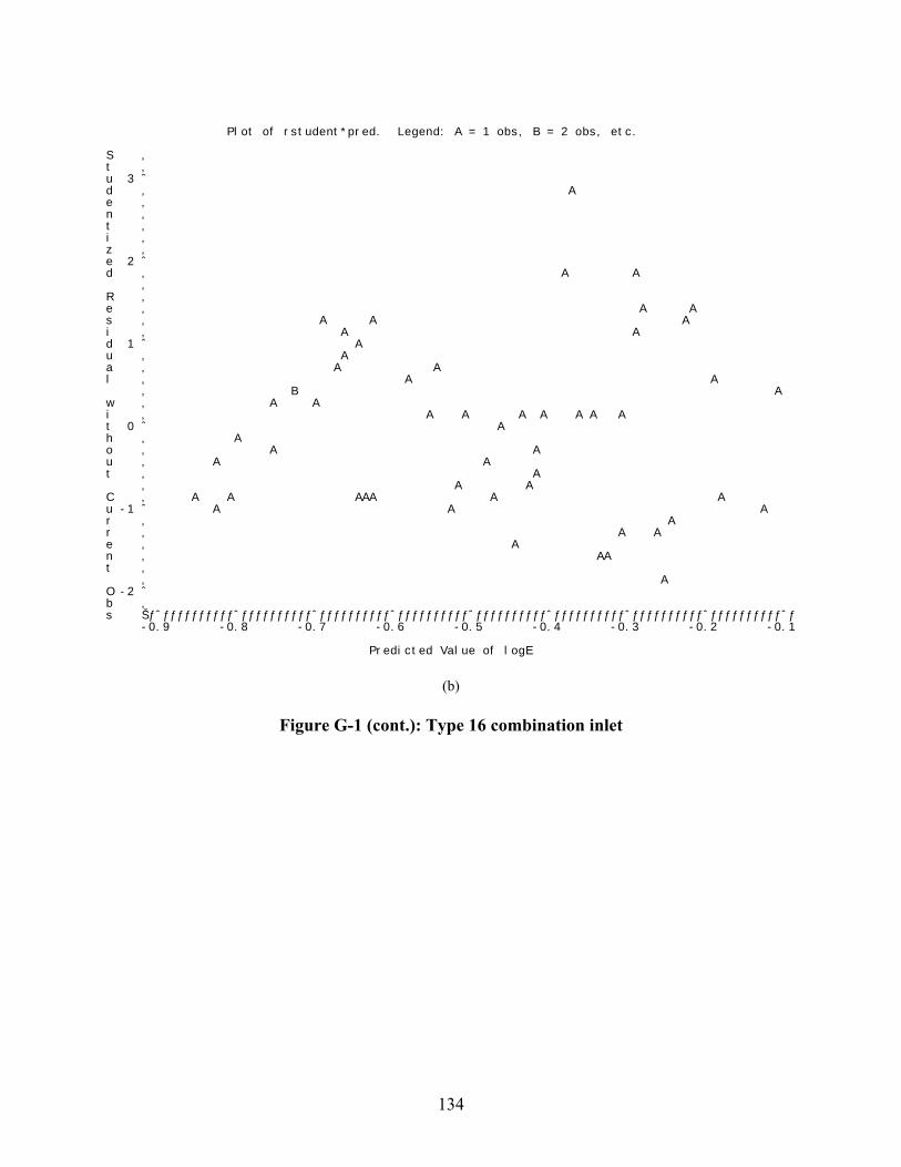
134
Plot of rstudent*pred. Legend: A = 1 obs, B = 2 obs, etc. S ‚ t ‚ u 3 ˆ d ‚ A e ‚ n ‚ t ‚ i ‚ z ‚ e 2 ˆ d ‚ A A ‚ R ‚ e ‚ A A s ‚ A A A i ‚ A A d 1 ˆ A u ‚ A a ‚ A A l ‚ A A ‚ B A w ‚ A A i ‚ A A A A A A A t 0 ˆ A h ‚ A o ‚ A A u ‚ A A t ‚ A ‚ A A C ‚ A A AAA A A u -1 ˆ A A A r ‚ A r ‚ A A e ‚ A n ‚ AA t ‚ ‚ A O -2 ˆ b ‚ s Šƒˆƒƒƒƒƒƒƒƒƒƒˆƒƒƒƒƒƒƒƒƒƒˆƒƒƒƒƒƒƒƒƒƒˆƒƒƒƒƒƒƒƒƒƒˆƒƒƒƒƒƒƒƒƒƒˆƒƒƒƒƒƒƒƒƒƒˆƒƒƒƒƒƒƒƒƒƒˆƒƒƒƒƒƒƒƒƒƒˆƒ -0.9 -0.8 -0.7 -0.6 -0.5 -0.4 -0.3 -0.2 -0.1 Predicted Value of logE
(b)
Figure G-1 (cont.): Type 16 combination inlet
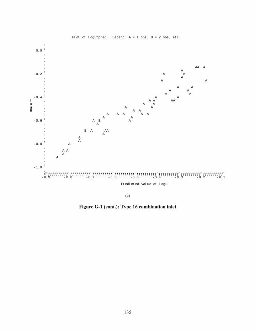
135
Plot of logE*pred. Legend: A = 1 obs, B = 2 obs, etc. ‚ ‚ 0.0 ˆ ‚ ‚ ‚ ‚ ‚ AA A ‚ A -0.2 ˆ A A ‚ A ‚ A A ‚ ‚ A A ‚ A A ‚ A A -0.4 ˆ A A l ‚ A A AA o ‚ A A g ‚ A A E ‚ A A ‚ A A A A A ‚ A A -0.6 ˆ A B A ‚ A ‚ ‚ B A AA ‚ A ‚ A ‚ A -0.8 ˆ A ‚ ‚ A A ‚ A ‚ A ‚ ‚ -1.0 ˆ ‚ Šˆƒƒƒƒƒƒƒƒƒƒˆƒƒƒƒƒƒƒƒƒƒˆƒƒƒƒƒƒƒƒƒƒˆƒƒƒƒƒƒƒƒƒƒˆƒƒƒƒƒƒƒƒƒƒˆƒƒƒƒƒƒƒƒƒƒˆƒƒƒƒƒƒƒƒƒƒˆƒƒƒƒƒƒƒƒƒƒˆ -0.9 -0.8 -0.7 -0.6 -0.5 -0.4 -0.3 -0.2 -0.1
Predicted Value of logE
(c)
Figure G-1 (cont.): Type 16 combination inlet

136
The REG Procedure Model: MODEL1 Dependent Variable: logE Number of Observations Read 53 Number of Observations Used 53 Analysis of Variance Sum of Mean Source DF Squares Square F Value Pr > F Model 3 3.81553 1.27184 325.37 <.0001 Error 49 0.19154 0.00391 Corrected Total 52 4.00707 Root MSE 0.06252 R-Square 0.9522 Dependent Mean -0.54874 Adj R-Sq 0.9493 Coeff Var -11.39360 Parameter Estimates Parameter Standard Variable Label DF Estimate Error t Value Pr > |t| Intercept Intercept 1 -1.20291 0.03673 -32.75 <.0001 logLh logLh 1 0.66466 0.11875 5.60 <.0001 logFr logFr 1 0.83532 0.08911 9.37 <.0001 log3 log3 1 -1.13773 0.08641 -13.17 <.0001 Correlation of Estimates Variable Intercept logLh logFr log3 Intercept 1.0000 0.3470 -0.0169 -0.1383 logLh 0.3470 1.0000 0.9139 -0.9661 logFr -0.0169 0.9139 1.0000 -0.9385 log3 -0.1383 -0.9661 -0.9385 1.0000
Note: logLh = log(h/L), logFr = log(V2T/gA), log3 = log(V2/gL)
(a)
Figure G-2: Type 13 combination inlet

137
Plot of rstudent*pred. Legend: A = 1 obs, B = 2 obs, etc. S ‚ t ‚ u 2.0 ˆ A d ‚ A e ‚ n ‚ A t 1.5 ˆ A A i ‚ B z ‚ e ‚ A A d 1.0 ˆ ‚ A A R ‚ A A A e ‚ A A A s 0.5 ˆ A A i ‚ A A d ‚ A A AA u ‚ A A A A A a 0.0 ˆ l ‚ A ‚ w ‚ A i -0.5 ˆ A A A t ‚ h ‚ A A A A o ‚ A A u -1.0 ˆ A A t ‚ A A ‚ A AA C ‚ A u -1.5 ˆ A A r ‚ r ‚ e ‚ A n -2.0 ˆ t ‚ A ‚ O ‚ b -2.5 ˆ s ‚ Šƒƒˆƒƒƒƒƒƒƒƒƒƒƒƒƒˆƒƒƒƒƒƒƒƒƒƒƒƒƒˆƒƒƒƒƒƒƒƒƒƒƒƒƒˆƒƒƒƒƒƒƒƒƒƒƒƒƒˆƒƒƒƒƒƒƒƒƒƒƒƒƒˆƒƒƒƒƒƒƒƒƒƒƒƒƒˆƒƒ -1.2 -1.0 -0.8 -0.6 -0.4 -0.2 0.0 Predicted Value of logE
(b)
Figure G-2 (cont.): Type 13 combination inlet
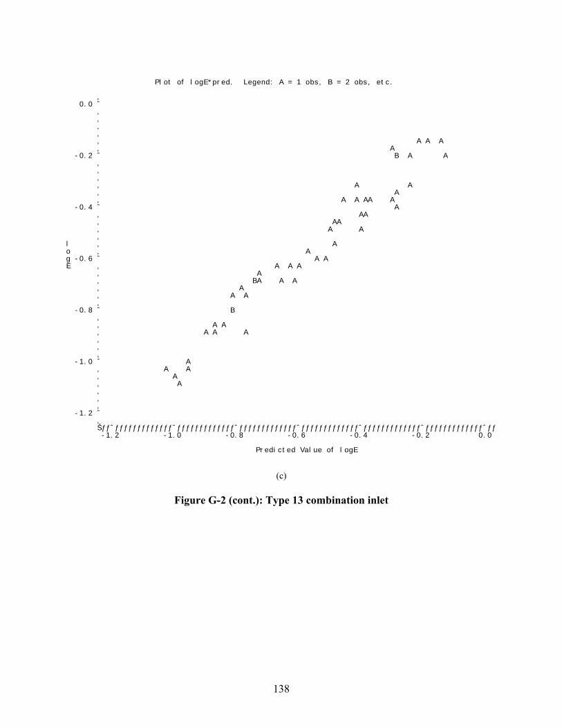
138
Plot of logE*pred. Legend: A = 1 obs, B = 2 obs, etc. ‚ 0.0 ˆ ‚ ‚ ‚ ‚ ‚ A A A ‚ A -0.2 ˆ B A A ‚ ‚ ‚ ‚ A A ‚ A ‚ A A AA A -0.4 ˆ A ‚ AA ‚ AA ‚ A A ‚ l ‚ A o ‚ A g -0.6 ˆ A A E ‚ A A A ‚ A ‚ BA A A ‚ A ‚ A A ‚ -0.8 ˆ B ‚ ‚ A A ‚ A A A ‚ ‚ ‚ -1.0 ˆ A ‚ A A ‚ A ‚ A ‚ ‚ ‚ -1.2 ˆ ‚ Šƒƒˆƒƒƒƒƒƒƒƒƒƒƒƒƒˆƒƒƒƒƒƒƒƒƒƒƒƒƒˆƒƒƒƒƒƒƒƒƒƒƒƒƒˆƒƒƒƒƒƒƒƒƒƒƒƒƒˆƒƒƒƒƒƒƒƒƒƒƒƒƒˆƒƒƒƒƒƒƒƒƒƒƒƒƒˆƒƒ -1.2 -1.0 -0.8 -0.6 -0.4 -0.2 0.0
Predicted Value of logE
(c)
Figure G-2 (cont.): Type 13 combination inlet
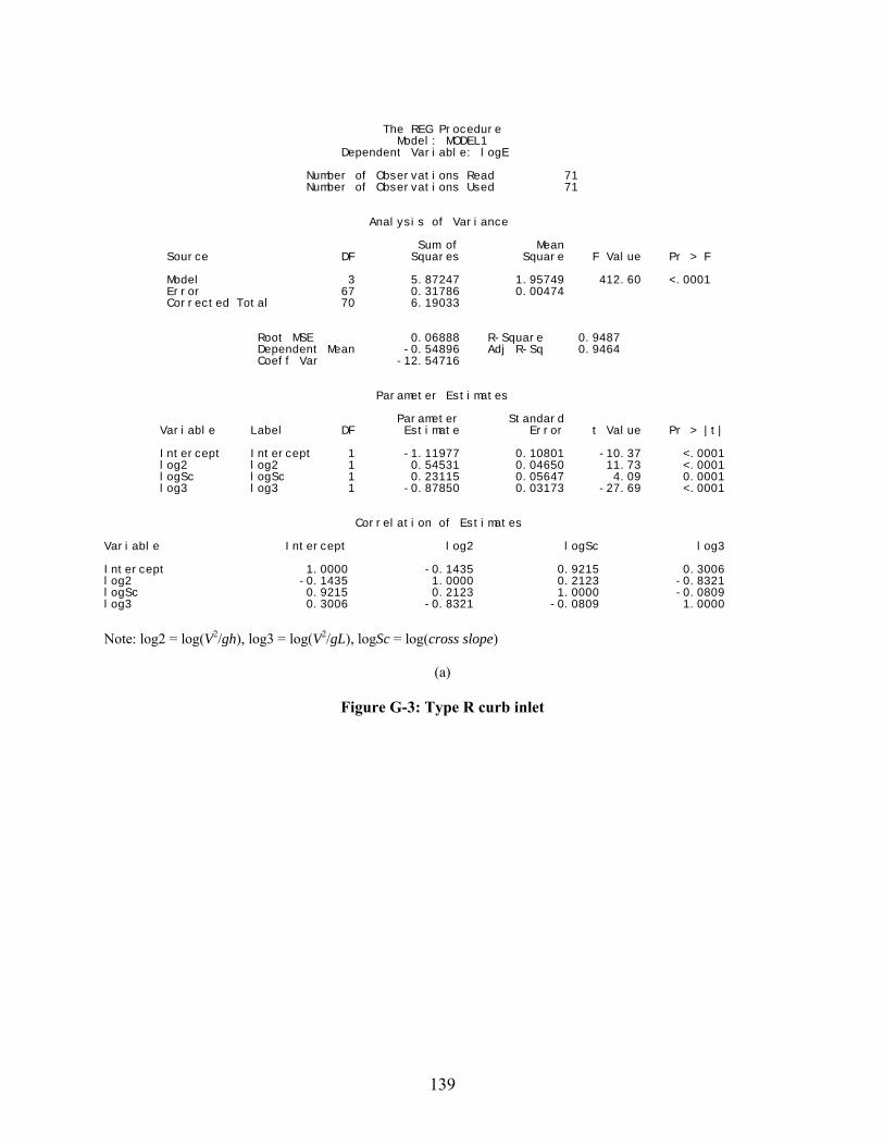
139
The REG Procedure Model: MODEL1 Dependent Variable: logE Number of Observations Read 71 Number of Observations Used 71 Analysis of Variance Sum of Mean Source DF Squares Square F Value Pr > F Model 3 5.87247 1.95749 412.60 <.0001 Error 67 0.31786 0.00474 Corrected Total 70 6.19033 Root MSE 0.06888 R-Square 0.9487 Dependent Mean -0.54896 Adj R-Sq 0.9464 Coeff Var -12.54716 Parameter Estimates Parameter Standard Variable Label DF Estimate Error t Value Pr > |t| Intercept Intercept 1 -1.11977 0.10801 -10.37 <.0001 log2 log2 1 0.54531 0.04650 11.73 <.0001 logSc logSc 1 0.23115 0.05647 4.09 0.0001 log3 log3 1 -0.87850 0.03173 -27.69 <.0001 Correlation of Estimates Variable Intercept log2 logSc log3 Intercept 1.0000 -0.1435 0.9215 0.3006 log2 -0.1435 1.0000 0.2123 -0.8321 logSc 0.9215 0.2123 1.0000 -0.0809 log3 0.3006 -0.8321 -0.0809 1.0000
Note: log2 = log(V2/gh), log3 = log(V2/gL), logSc = log(cross slope)
(a)
Figure G-3: Type R curb inlet

140
Plot of rstudent*pred. Legend: A = 1 obs, B = 2 obs, etc. S ‚ t ‚ u 2.5 ˆ d ‚ e ‚ A n ‚ A t 2.0 ˆ A i ‚ A z ‚ A e ‚ A d 1.5 ˆ A AA ‚ R ‚ e ‚ A A A s 1.0 ˆ B i ‚ A d ‚ A u ‚ A a 0.5 ˆ A A AA A l ‚ A ‚ A A A A A w ‚ A A A A A i 0.0 ˆ A A A A A t ‚ A AA AA h ‚ A o ‚ A u -0.5 ˆ A A A t ‚ A A A ‚ B A C ‚ A A A u -1.0 ˆ A A A r ‚ A r ‚ A A A e ‚ A A n -1.5 ˆ A t ‚ A ‚ A A O ‚ A b -2.0 ˆ s ‚ Šƒƒˆƒƒƒƒƒƒƒƒƒƒƒˆƒƒƒƒƒƒƒƒƒƒƒˆƒƒƒƒƒƒƒƒƒƒƒˆƒƒƒƒƒƒƒƒƒƒƒˆƒƒƒƒƒƒƒƒƒƒƒˆƒƒƒƒƒƒƒƒƒƒƒˆƒƒƒƒƒƒƒƒƒƒƒˆƒƒ -1.2 -1.0 -0.8 -0.6 -0.4 -0.2 0.0 0.2 Predicted Value of logE
(b)
Figure G-3 (cont.): Type R curb inlet
141
Plot of logE*pred. Legend: A = 1 obs, B = 2 obs, etc. ‚ 0.0 ˆ ‚ ‚ A A ‚ B A A ‚ ‚ AA A ‚ -0.2 ˆ A A ‚ A A ‚ ‚ A A ‚ A AA ‚ AAA ‚ BA -0.4 ˆ A ‚ A A A ‚ A B A ‚ A ‚ A A A l ‚ o ‚ A A g -0.6 ˆ AA A E ‚ A A ‚ A A ‚ A ‚ AA A A ‚ B AA ‚ AA -0.8 ˆ ‚ AA A A ‚ ‚ A ‚ ‚ B C ‚ -1.0 ˆ ‚ ‚ ‚ A ‚ A A ‚ A ‚ A -1.2 ˆ Šƒƒˆƒƒƒƒƒƒƒƒƒƒƒˆƒƒƒƒƒƒƒƒƒƒƒˆƒƒƒƒƒƒƒƒƒƒƒˆƒƒƒƒƒƒƒƒƒƒƒˆƒƒƒƒƒƒƒƒƒƒƒˆƒƒƒƒƒƒƒƒƒƒƒˆƒƒƒƒƒƒƒƒƒƒƒˆƒƒ -1.2 -1.0 -0.8 -0.6 -0.4 -0.2 0.0 0.2
Predicted Value of loge
(c)
Figure G-3 (cont.): Type R curb inlet

142

143
APPENDIX H
CALCULATED EFFICIENCY

144

145
H.1 Efficiency Determined from Empirical Equations and Improved
UDFCD Methods
Table H-1: Type 13 combination-inlet calculated efficiency
Efficiency Test ID Number
Depth
(ft) Grates
Flow (cfs) Observed Regression UDFCD New
62 0.333 1 4.83 0.61 0.51 0.50 63 0.501 1 26.19 0.24 0.21 0.30 64 0.999 1 126.42 0.10 0.11 0.17 91 0.333 1 2.96 0.63 0.58 0.64 92 0.501 1 10.13 0.38 0.40 0.48 93 0.999 1 95.09 0.13 0.13 0.22
146 0.333 1 15.90 0.27 0.27 0.20 147 0.501 1 33.67 0.20 0.18 0.24 148 0.999 1 166.64 0.09 0.09 0.08 161 0.333 1 7.79 0.50 0.39 0.36 162 0.501 1 24.78 0.24 0.23 0.23 163 0.999 1 155.88 0.09 0.10 0.07 227 0.333 1 12.94 0.25 0.30 0.26 228 0.501 1 37.72 0.13 0.17 0.21 229 0.999 1 142.63 0.08 0.10 0.13 242 0.333 1 9.04 0.43 0.34 0.32 243 0.501 1 27.28 0.21 0.22 0.21 244 0.999 1 129.69 0.09 0.11 0.13 59 0.333 2 4.68 0.73 0.72 0.73 60 0.501 2 22.60 0.36 0.32 0.49 61 0.999 2 127.82 0.16 0.15 0.25
104 0.333 2 3.27 0.62 0.75 0.84 105 0.501 2 11.22 0.44 0.53 0.72 106 0.999 2 98.20 0.20 0.18 0.36 149 0.333 2 14.34 0.34 0.40 0.33 150 0.501 2 33.67 0.24 0.25 0.34 151 0.999 2 176.61 0.13 0.12 0.12 158 0.333 2 8.11 0.63 0.53 0.56 159 0.501 2 23.38 0.35 0.34 0.42 160 0.999 2 161.34 0.14 0.13 0.14 230 0.333 2 13.25 0.38 0.42 0.36 231 0.501 2 36.63 0.21 0.24 0.31 232 0.999 2 138.73 0.13 0.14 0.22 239 0.333 2 8.26 0.66 0.51 0.55 240 0.501 2 26.03 0.33 0.32 0.38 241 0.999 2 127.82 0.16 0.15 0.25 56 0.333 3 4.36 0.82 0.91 0.86 57 0.501 3 20.58 0.43 0.41 0.67 58 0.999 3 126.57 0.23 0.18 0.35
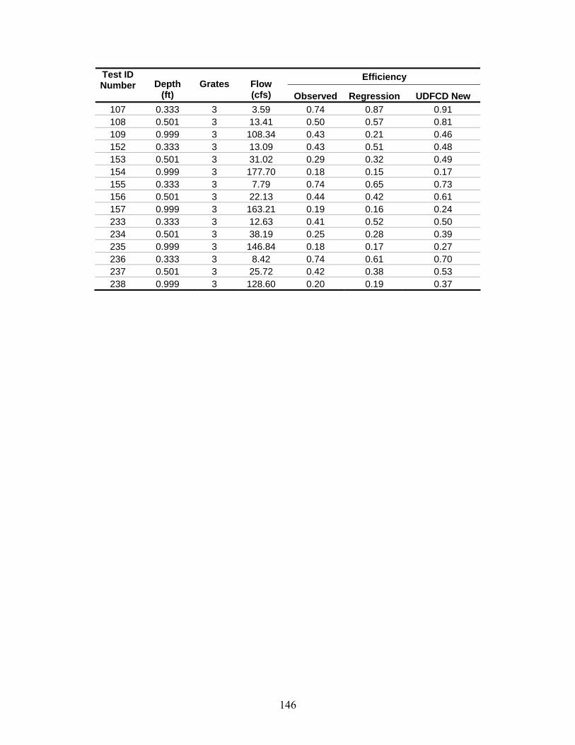
146
Efficiency Test ID Number
Depth
(ft) Grates
Flow (cfs) Observed Regression UDFCD New
107 0.333 3 3.59 0.74 0.87 0.91 108 0.501 3 13.41 0.50 0.57 0.81 109 0.999 3 108.34 0.43 0.21 0.46 152 0.333 3 13.09 0.43 0.51 0.48 153 0.501 3 31.02 0.29 0.32 0.49 154 0.999 3 177.70 0.18 0.15 0.17 155 0.333 3 7.79 0.74 0.65 0.73 156 0.501 3 22.13 0.44 0.42 0.61 157 0.999 3 163.21 0.19 0.16 0.24 233 0.333 3 12.63 0.41 0.52 0.50 234 0.501 3 38.19 0.25 0.28 0.39 235 0.999 3 146.84 0.18 0.17 0.27 236 0.333 3 8.42 0.74 0.61 0.70 237 0.501 3 25.72 0.42 0.38 0.53 238 0.999 3 128.60 0.20 0.19 0.37

147
Table H-2: Type 16 combination-inlet calculated efficiency
Efficiency Test ID Number
Depth
(ft) Grates
Flow (cfs) Observed Regression UDFCD New
65 0.333 1 5.14 0.61 0.51 0.56 66 0.501 1 21.36 0.28 0.28 0.39 67 0.999 1 126.89 0.14 0.16 0.25 80 0.333 1 3.74 0.50 0.49 0.63 81 0.501 1 11.54 0.35 0.38 0.40 82 0.999 1 95.55 0.17 0.18 0.20
143 0.333 1 15.28 0.29 0.36 0.40 144 0.501 1 33.98 0.21 0.24 0.27 145 0.999 1 176.61 0.12 0.14 0.07 174 0.333 1 7.95 0.55 0.41 0.46 175 0.501 1 22.29 0.31 0.31 0.29 176 0.999 1 162.89 0.13 0.15 0.06 224 0.333 1 13.09 0.33 0.38 0.33 225 0.501 1 37.88 0.20 0.23 0.18 226 0.999 1 141.23 0.14 0.15 -0.08 263 0.333 1 7.48 0.65 0.43 0.37 264 0.501 1 28.06 0.32 0.29 0.21 265 0.999 1 129.38 0.16 0.16 -0.05 68 0.333 2 5.30 0.71 0.65 0.78 69 0.501 2 23.23 0.34 0.34 0.58 70 0.999 2 124.70 0.21 0.20 0.34 77 0.333 2 3.27 0.57 0.66 0.84 78 0.501 2 11.22 0.40 0.49 0.73 79 0.999 2 94.46 0.20 0.23 0.37
140 0.333 2 14.65 0.36 0.46 0.59 141 0.501 2 32.73 0.27 0.31 0.38 142 0.999 2 177.08 0.19 0.18 0.13 185 0.333 2 7.95 0.65 0.52 0.69 186 0.501 2 23.69 0.37 0.38 0.47 187 0.999 2 163.67 0.20 0.19 0.15 221 0.333 2 13.25 0.38 0.48 0.48 222 0.501 2 36.63 0.25 0.29 0.26 223 0.999 2 144.97 0.20 0.19 -0.04 266 0.333 2 8.73 0.68 0.52 0.57 267 0.501 2 26.50 0.38 0.37 0.35 268 0.999 2 130.94 0.25 0.20 0.01 71 0.333 3 4.52 0.83 0.78 0.89 72 0.501 3 23.69 0.40 0.39 0.73 73 0.999 3 125.80 0.27 0.23 0.45 74 0.333 3 3.43 0.64 0.74 0.92 75 0.501 3 11.22 0.47 0.56 0.86 76 0.999 3 93.84 0.28 0.26 0.53
137 0.333 3 13.25 0.45 0.55 0.74 138 0.501 3 39.91 0.31 0.33 0.49
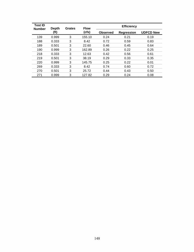
148
Efficiency Test ID Number
Depth
(ft) Grates
Flow (cfs) Observed Regression UDFCD New
139 0.999 3 155.10 0.24 0.21 0.19 188 0.333 3 8.42 0.72 0.59 0.83 189 0.501 3 22.60 0.46 0.45 0.64 190 0.999 3 162.89 0.26 0.22 0.25 218 0.333 3 12.63 0.42 0.56 0.61 219 0.501 3 38.19 0.29 0.33 0.35 220 0.999 3 145.75 0.25 0.22 0.01 269 0.333 3 8.42 0.74 0.60 0.72 270 0.501 3 25.72 0.44 0.43 0.50 271 0.999 3 127.82 0.29 0.24 0.08

149
Table H-3: Type R curb inlet calculated efficiency
Efficiency Test ID Number
Depth
(ft) Length
(ft) Flow (cfs) Observed Regression UDFCD New
44 0.333 15 4.36 0.89 0.95 0.95 45 0.501 15 20.26 0.51 0.51 0.55 46 0.999 15 128.76 0.24 0.22 0.22 47 0.333 12 3.90 0.84 0.84 0.87 48 0.501 12 21.82 0.38 0.41 0.43 49 0.999 12 126.26 0.20 0.18 0.18 50 0.333 9 4.21 0.70 0.62 0.70 51 0.501 9 21.51 0.35 0.32 0.34 52 0.999 9 127.82 0.15 0.14 0.14 53 0.333 5 4.36 0.50 0.36 0.43 54 0.501 5 22.29 0.24 0.19 0.19 55 0.999 5 125.48 0.08 0.08 0.08
122 0.333 15 3.27 0.90 1.00 1.00 123 0.501 15 10.91 0.60 0.78 0.71 124 0.999 15 94.31 0.31 0.30 0.27 119 0.333 12 2.81 0.83 1.00 0.96 120 0.501 12 10.91 0.53 0.64 0.60 121 0.999 12 93.84 0.25 0.25 0.22 116 0.333 9 3.12 0.65 0.79 0.81 117 0.501 9 11.22 0.47 0.49 0.46 118 0.999 9 93.84 0.19 0.19 0.17 110 0.333 5 2.96 0.58 0.49 0.53 111 0.501 5 11.07 0.39 0.29 0.28 112 0.999 5 93.22 0.12 0.11 0.09 125 0.333 15 14.81 0.44 0.45 0.58 126 0.501 15 33.51 0.30 0.38 0.40 127 0.999 15 178.48 0.18 0.18 0.18 128 0.333 12 13.41 0.43 0.40 0.50 129 0.501 12 32.89 0.27 0.31 0.33 130 0.999 12 176.14 0.15 0.15 0.14 131 0.333 9 13.41 0.36 0.31 0.39 132 0.501 9 29.62 0.23 0.26 0.27 133 0.999 9 173.03 0.11 0.11 0.11 134 0.333 5 13.09 0.25 0.19 0.23 135 0.501 5 28.37 0.16 0.16 0.16 136 0.999 5 178.95 0.08 0.07 0.06 203 0.333 15 7.01 0.84 0.72 0.82 204 0.501 15 21.51 0.49 0.50 0.50 205 0.999 15 166.79 0.19 0.20 0.19 200 0.333 12 7.48 0.71 0.57 0.68 201 0.501 12 21.67 0.42 0.40 0.42 202 0.999 12 166.79 0.15 0.17 0.15 197 0.333 9 6.24 0.65 0.44 0.61 198 0.501 9 21.82 0.34 0.31 0.32

150
Efficiency Test ID Number
Depth
(ft) Length
(ft) Flow (cfs) Observed Regression UDFCD New
199 0.999 9 166.01 0.12 0.13 0.12 191 0.333 5 7.33 0.38 0.30 0.31 192 0.501 5 22.91 0.18 0.18 0.18 193 0.999 5 166.01 0.07 0.08 0.07 206 0.333 15 13.09 0.44 0.49 0.59 207 0.501 15 38.35 0.27 0.35 0.37 208 0.999 15 143.41 0.19 0.20 0.19 209 0.333 12 12.63 0.42 0.41 0.50 210 0.501 12 38.35 0.24 0.28 0.30 211 0.999 12 152.92 0.15 0.16 0.15 212 0.333 9 13.87 0.35 0.30 0.37 213 0.501 9 38.19 0.19 0.22 0.23 214 0.999 9 141.54 0.12 0.13 0.12 215 0.333 5 13.72 0.22 0.18 0.22 216 0.501 5 38.19 0.11 0.13 0.13 217 0.999 5 140.29 0.07 0.08 0.07 284 0.333 15 7.79 0.80 0.72 0.75 285 0.501 15 23.38 0.46 0.47 0.47 286 0.999 15 123.15 0.21 0.25 0.21 281 0.333 12 8.73 0.70 0.55 0.61 282 0.501 12 25.25 0.38 0.37 0.37 283 0.999 12 113.79 0.18 0.22 0.18 278 0.333 9 7.95 0.63 0.45 0.50 279 0.501 9 25.88 0.30 0.28 0.28 280 0.999 9 117.69 0.13 0.16 0.13 272 0.333 5 8.11 0.35 0.27 0.29 273 0.501 5 26.66 0.17 0.16 0.16 274 0.999 5 118.94 0.08 0.10 0.07

151
ELECTRONIC DATA SUPPLEMENT
CONTENTS AND ORGANIZATION
(stored on a 16-GB SDHCTM card)
Folder Files and/or Sub-folders Client Final Report Microsoft Word® (.doc) and Adobe® Acrobat®
(.pdf) files for both single- and double-sided printing; and SureThing (.std) CD label file
Analysis Microsoft Excel® (.xls) files Data and Photographs* 0.5% long 1% cross
0.5% long 2% cross 2% long 1% cross 2% long 2% cross 4% long 1% cross 4% long 2% cross Additional model photographs Additional tests Grate-inlet combination pictures Inlet construction Sump tests
*The reader is referred to the UDFCD for obtaining photographs and video documentation.