Seminar Purpose
• Show the methodology for calculating the reliability indices using graphics and examples
• Define terms used in reliability studies such as LOLE, LOLP, EUE, FOR, PFOR, pdf, etc.
• Provide information to stakeholders concerning input data and interpretation of study results for single area and multi-area studies

Generation Adequacy Study Objectives
• Ensure installed generation reserve is sufficient• Test the sensitivity of study parameters
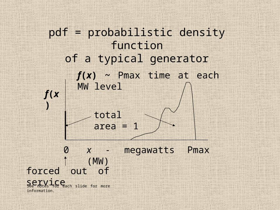
pdf = probabilistic density functionof a typical generator
forced out of service
f(x)
x - megawatts (MW)
total area = 1
0 Pmax
f(x) ~ Pmax time at each MW level
See notes for each slide for more information.
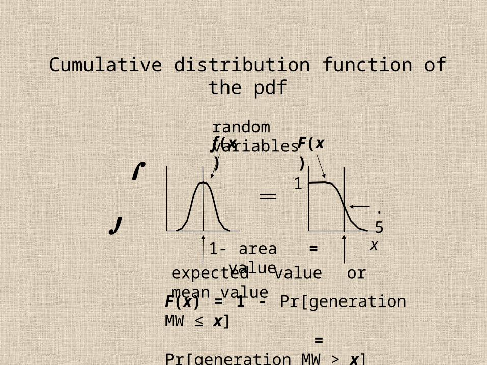
Cumulative distribution function of the pdf
random variables
x
1
f(x) F(x)
expected value or mean value
1- area = value
F(x) = 1 - Pr[generation MW ≤ x] = Pr[generation MW > x]
.5
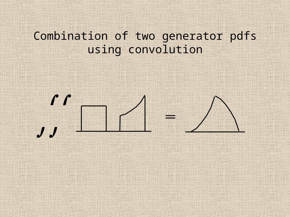
Combination of two generator pdfs using convolution
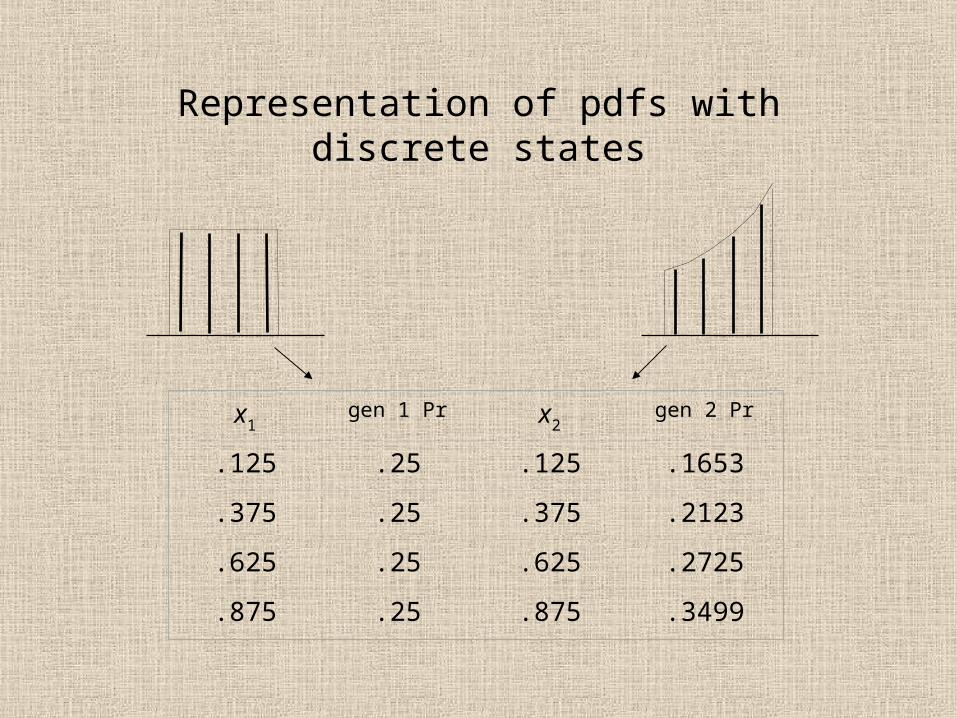
Representation of pdfs with discrete states
x1 gen 1 Pr x2 gen 2 Pr
.125 .25 .125 .1653
.375 .25 .375 .2123
.625 .25 .625 .2725
.875 .25 .875 .3499
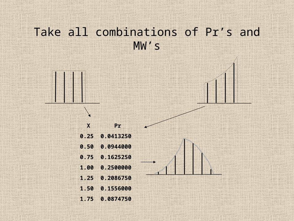
Take all combinations of Pr’s and MW’s
X Pr
0.25 0.0413250
0.50 0.0944000
0.75 0.1625250
1.00 0.2500000
1.25 0.2086750
1.50 0.1556000
1.75 0.0874750
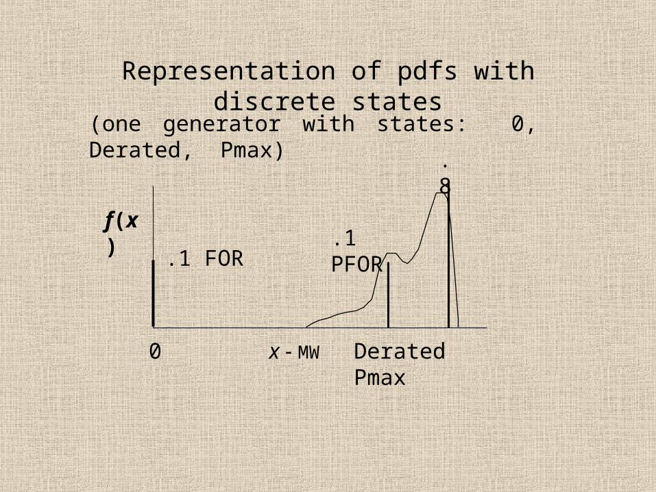
Representation of pdfs with discrete states
(one generator with states: 0, Derated, Pmax)
f(x)
x - MW0 Derated Pmax
.8
.1 PFOR.1 FOR
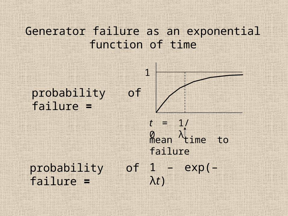
Generator failure as an exponential function of time
probability of failure =
1
t = 0
probability of failure =
1/λ
mean time to failure
1 – exp(–λt)
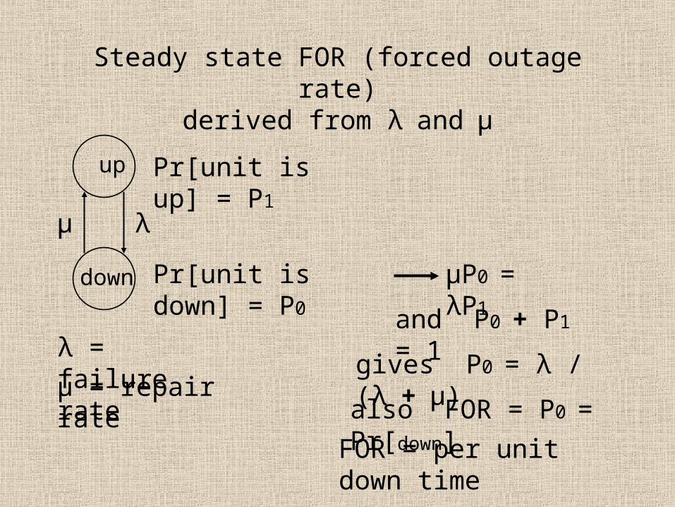
Steady state FOR (forced outage rate)derived from λ and µ
up
down
λµ
λ = failure rate
µ = repair rate
Pr[unit is up] = P1
Pr[unit is down] = P0
and P0 + P1 = 1
µP0 = λP1
gives P0 = λ / (λ + µ)
also FOR = P0 = Pr[down]
FOR = per unit down time
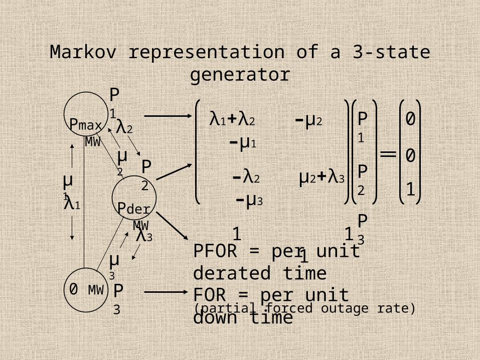
Markov representation of a 3-state generator
Pmax MW
0 MW
λ1
µ1
P1
Pder MW
P3
P2µ2
µ3
λ2
λ3
λ1+λ2 –µ2 –µ1
–λ2 µ2+λ3 –µ3
1 1 1
P1
P2
P3
0
0
1
FOR = per unit down time
PFOR = per unit derated time (partial forced outage rate)
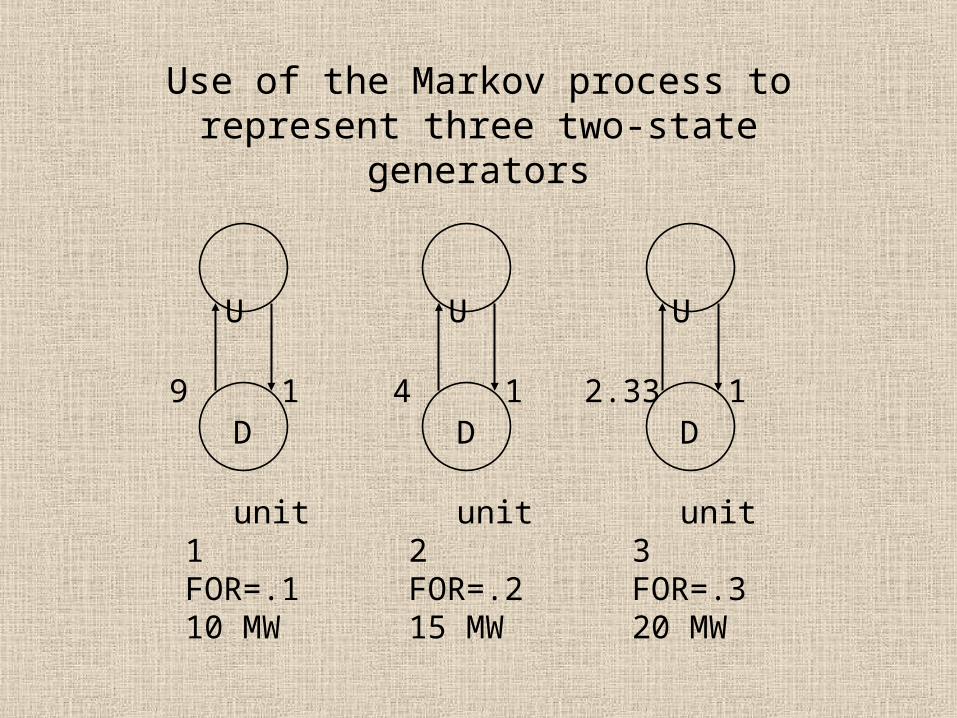
Use of the Markov process to represent three two-state generators
U
D
9 1
unit 1FOR=.110 MW
U
D
4 1
unit 2FOR=.215 MW
U
D
2.33 1
unit 3FOR=.320 MW
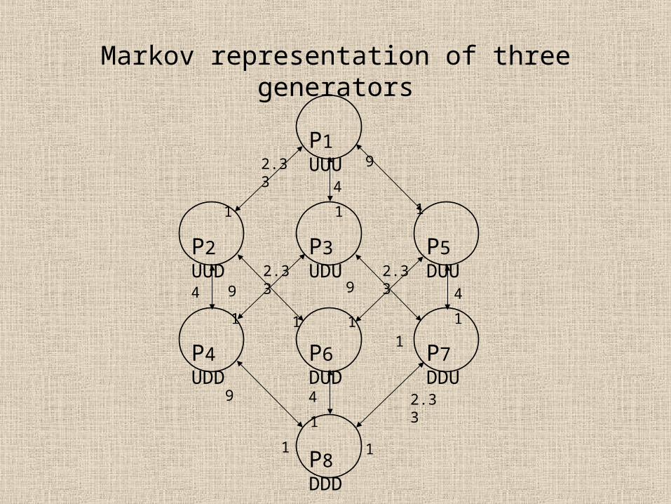
Markov representation of three generators
P3UDU
P2UUD
P1UUU
P5DUU
P6DUD
P4UDD
P8DDD
P7DDU
2.33
2.33 2.33
2.33
9
9
9
4
4 4
4
1 1 1
1 1
1
1 1
1
9
1 1
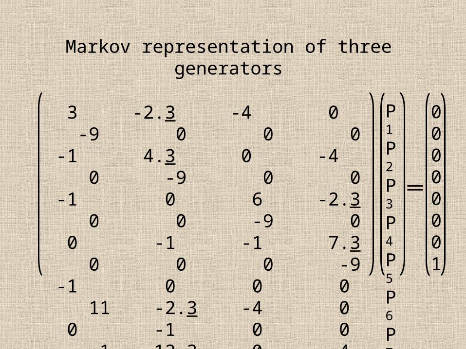
Markov representation of three generators
P1
P2
P3
P4
P5
P6
P7
P8
00000001
3 -2.3 -4 0 -9 0 0 0 -1 4.3 0 -4 0 -9 0 0 -1 0 6 -2.3 0 0 -9 0 0 -1 -1 7.3 0 0 0 -9 -1 0 0 0 11 -2.3 -4 0 0 -1 0 0 -1 12.3 0 -4 0 0 -1 0 -1 0 14 -2.3 1 1 1 1 1 1 1 1
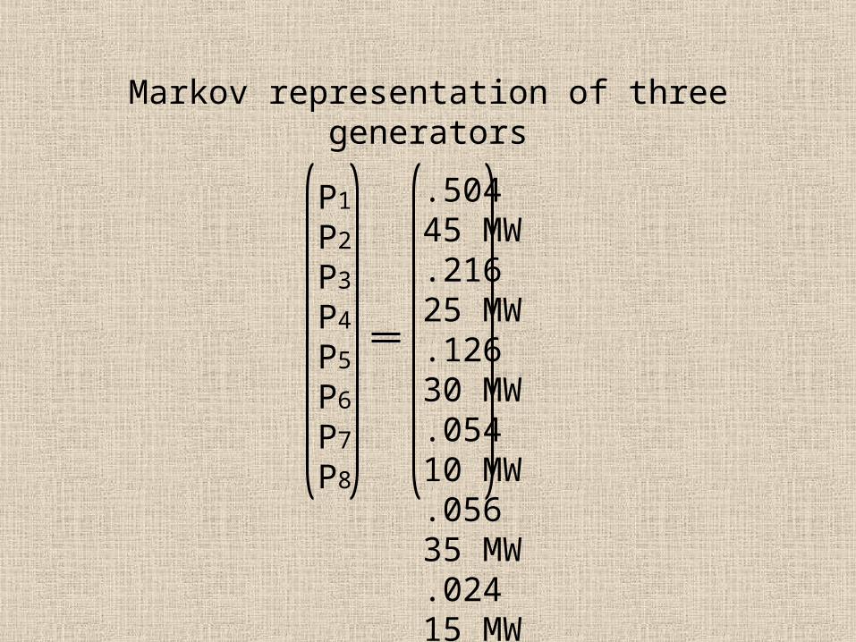
Markov representation of three generators
P1
P2
P3
P4
P5
P6
P7
P8
.504 45 MW
.216 25 MW
.126 30 MW
.054 10 MW
.056 35 MW
.024 15 MW
.014 20 MW
.006 0 MW
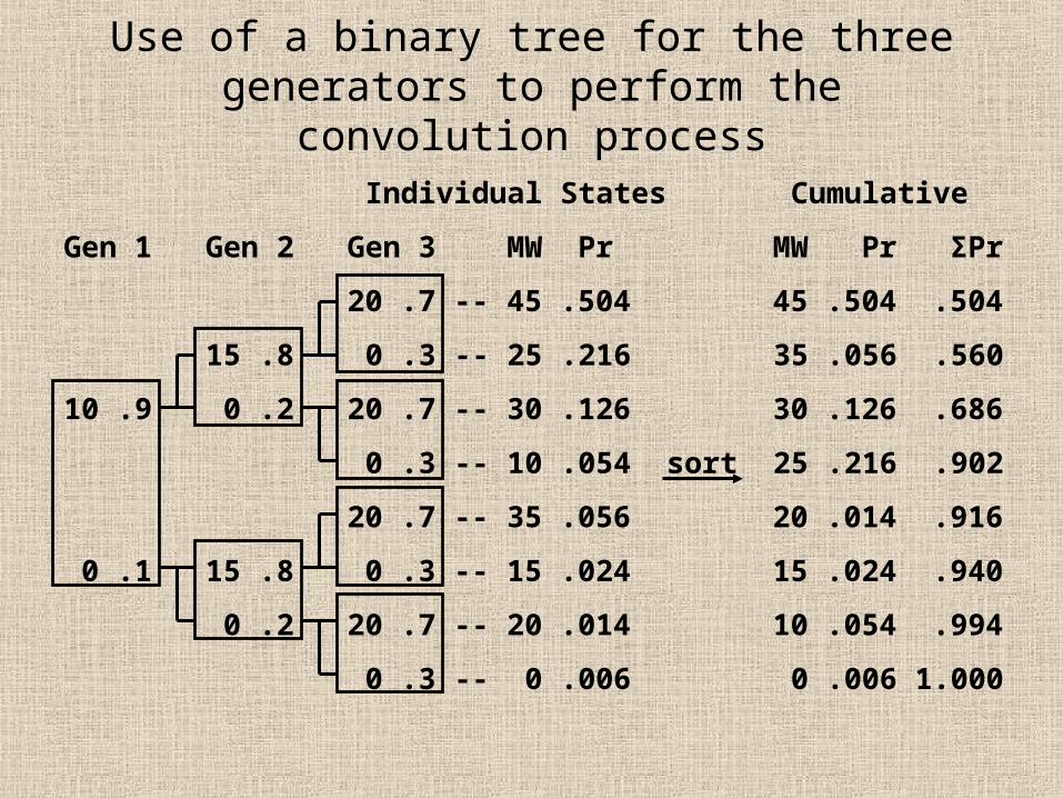
Use of a binary tree for the three generators to perform the convolution process
Individual States Cumulative
Gen 1 Gen 2 Gen 3 MW Pr MW Pr ΣPr
20 .7 -- 45 .504 45 .504 .504
15 .8 0 .3 -- 25 .216 35 .056 .560
10 .9 0 .2 20 .7 -- 30 .126 30 .126 .686
0 .3 -- 10 .054 sort 25 .216 .902
20 .7 -- 35 .056 20 .014 .916
0 .1 15 .8 0 .3 -- 15 .024 15 .024 .940
0 .2 20 .7 -- 20 .014 10 .054 .994
0 .3 -- 0 .006 0 .006 1.000
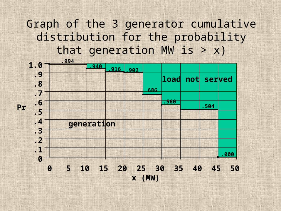
Graph of the 3 generator cumulative distribution for the probability that generation MW is > x)
1.0 .9 .8 .7 .6 .5 .4 .3 .2 .1 0 0 5 10 15 20 25 30 35 40 45 50 x (MW)
Pr
.994.940 .916 .902
.686
.560.504
.000
load not served
generation

Unsuitability of the binary tree and Markov methods for large systems
A system with 400 two-state generators has a total of:
400 120
2 10 states (combinations)
This is greater than the number of atoms in the universe (~1080)!
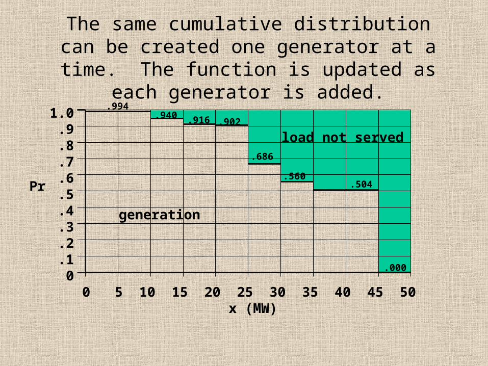
The same cumulative distribution can be created one generator at a time. The function is
updated as each generator is added.
1.0 .9 .8 .7 .6 .5 .4 .3 .2 .1 0 0 5 10 15 20 25 30 35 40 45 50 x (MW)
Pr
.994.940 .916 .902
.686
.560.504
.000
load not served
generation
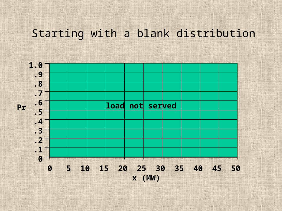
Starting with a blank distribution
1.0 .9 .8 .7 .6 .5 .4 .3 .2 .1 0 0 5 10 15 20 25 30 35 40 45 50 x (MW)
Pr load not served
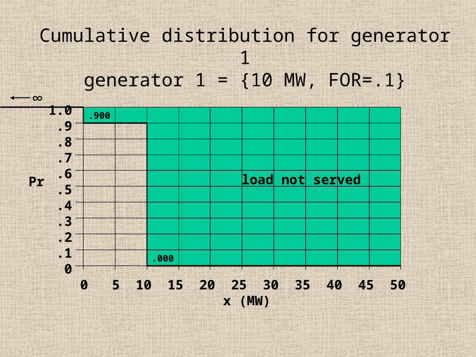
Cumulative distribution for generator 1generator 1 = {10 MW, FOR=.1}
Pr
1.0 .9 .8 .7 .6 .5 .4 .3 .2 .1 0 0 5 10 15 20 25 30 35 40 45 50 x (MW)
.900
load not served
.000
∞
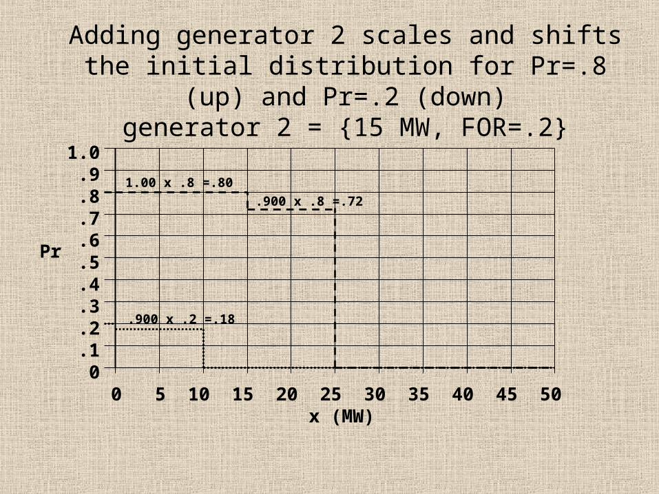
Adding generator 2 scales and shifts the initial distribution for Pr=.8 (up) and Pr=.2 (down)
generator 2 = {15 MW, FOR=.2}
1.0 .9 .8 .7 .6 .5 .4 .3 .2 .1 0 0 5 10 15 20 25 30 35 40 45 50 x (MW)
Pr
.900 x .2 =.18
.900 x .8 =.72
1.00 x .8 =.80
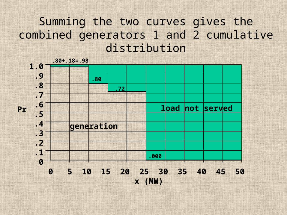
Summing the two curves gives the combined generators 1 and 2 cumulative distribution
1.0 .9 .8 .7 .6 .5 .4 .3 .2 .1 0 0 5 10 15 20 25 30 35 40 45 50 x (MW)
Pr load not served
.000
.72
.80+.18=.98
.80
generation
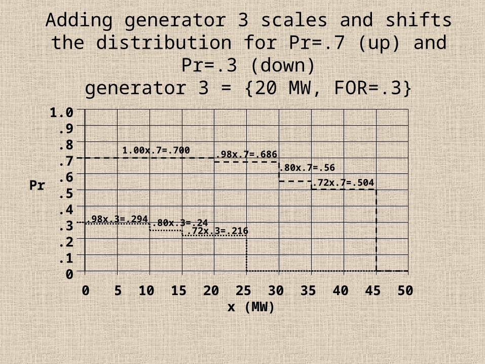
Adding generator 3 scales and shifts the distribution for Pr=.7 (up) and Pr=.3 (down)generator 3 = {20 MW, FOR=.3}
1.0 .9 .8 .7 .6 .5 .4 .3 .2 .1 0 0 5 10 15 20 25 30 35 40 45 50 x (MW)
Pr
.98x.3=.294 .80x.3=.24.72x.3=.216
.98x.7=.686
.80x.7=.56
.72x.7=.504
1.00x.7=.700
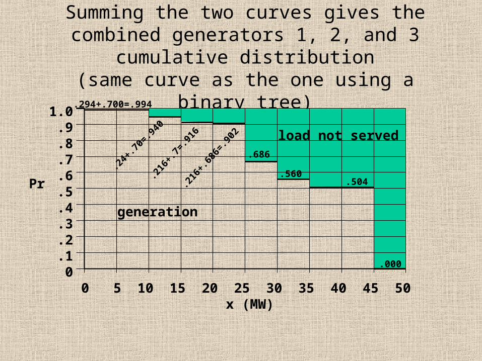
Summing the two curves gives the combined generators 1, 2, and 3 cumulative distribution(same curve as the one using a binary tree)
1.0 .9 .8 .7 .6 .5 .4 .3 .2 .1 0 0 5 10 15 20 25 30 35 40 45 50 x (MW)
Pr
.294+.700=.994
.24+.70=.940
.216+.7=.916
.686
.560.504
.000
load not served
generation
.216+.686=.902
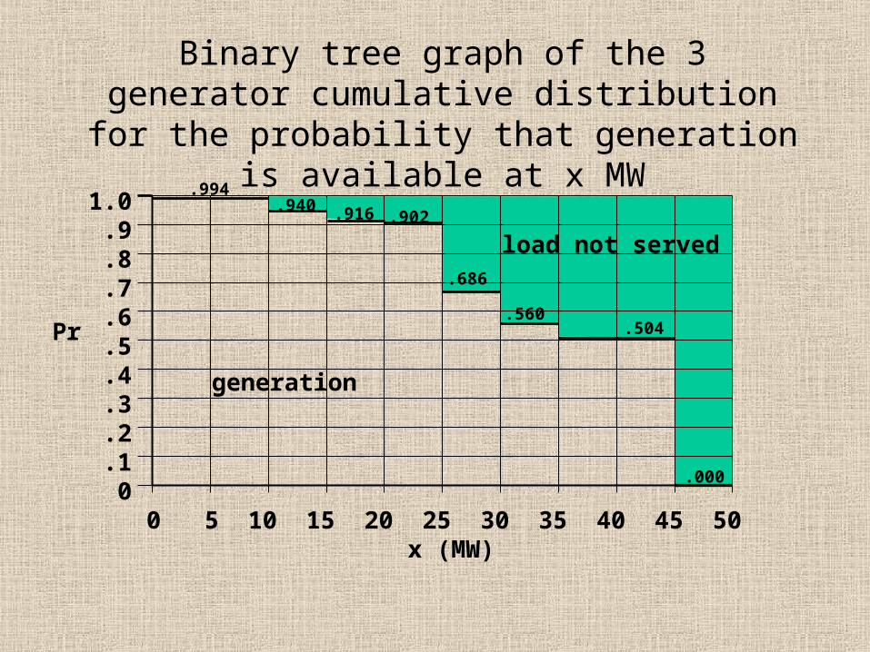
Binary tree graph of the 3 generator cumulative distribution for the probability that generation is
available at x MW1.0 .9 .8 .7 .6 .5 .4 .3 .2 .1 0 0 5 10 15 20 25 30 35 40 45 50 x (MW)
Pr
.994.940 .916 .902
.686
.560.504
.000
load not served
generation
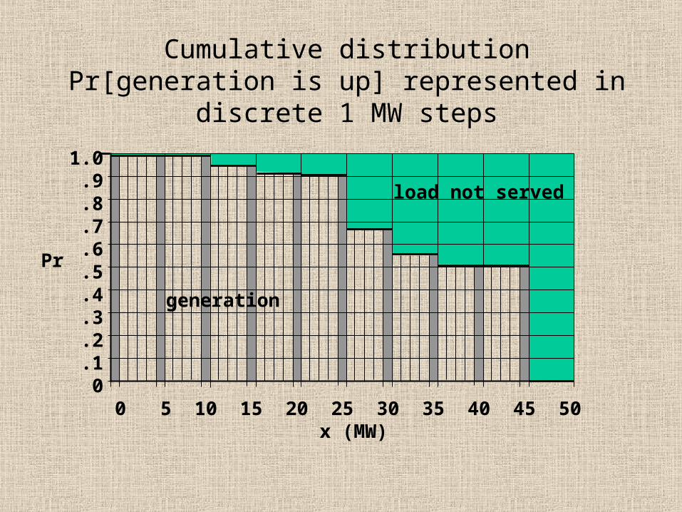
Cumulative distribution Pr[generation is up] represented in discrete 1 MW steps
1.0 .9 .8 .7 .6 .5 .4 .3 .2 .1 0 0 5 10 15 20 25 30 35 40 45 50 x (MW)
Pr
load not served
generation
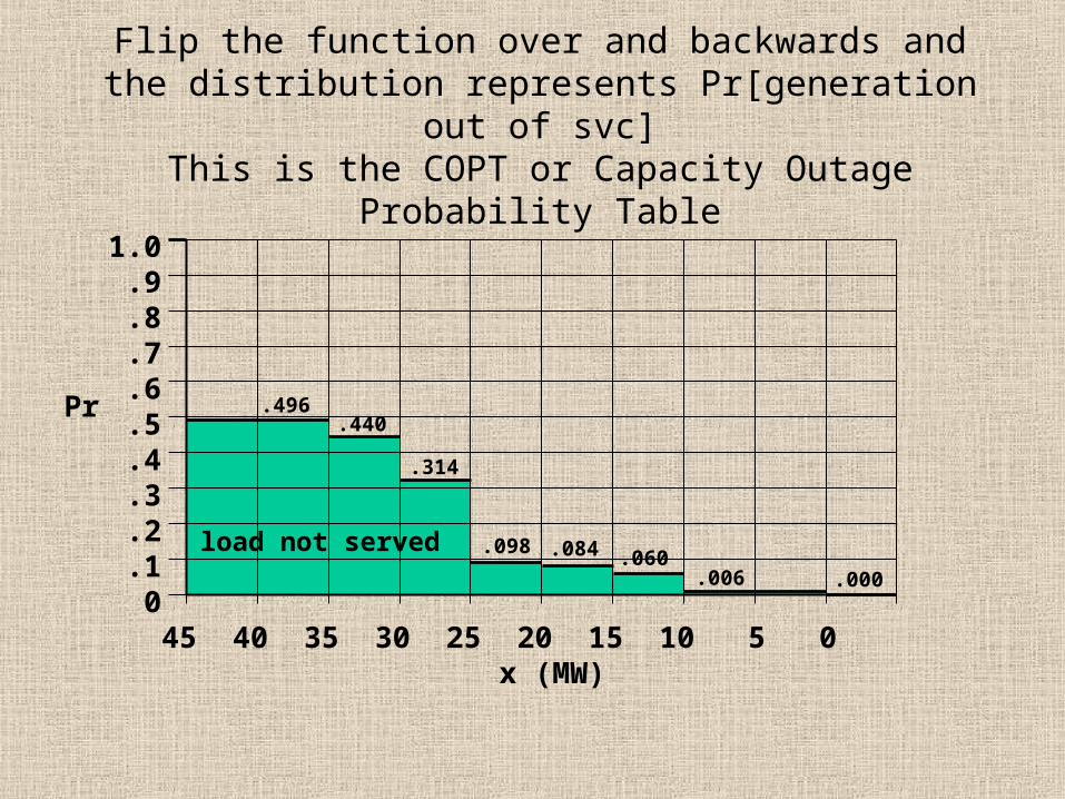
Flip the function over and backwards and the distribution represents Pr[generation out of svc]
This is the COPT or Capacity Outage Probability Table
1.0 .9 .8 .7 .6 .5 .4 .3 .2 .1 0 45 40 35 30 25 20 15 10 5 0 x (MW)
Pr
load not served
.496.440
.314
.098 .084 .060.006 .000
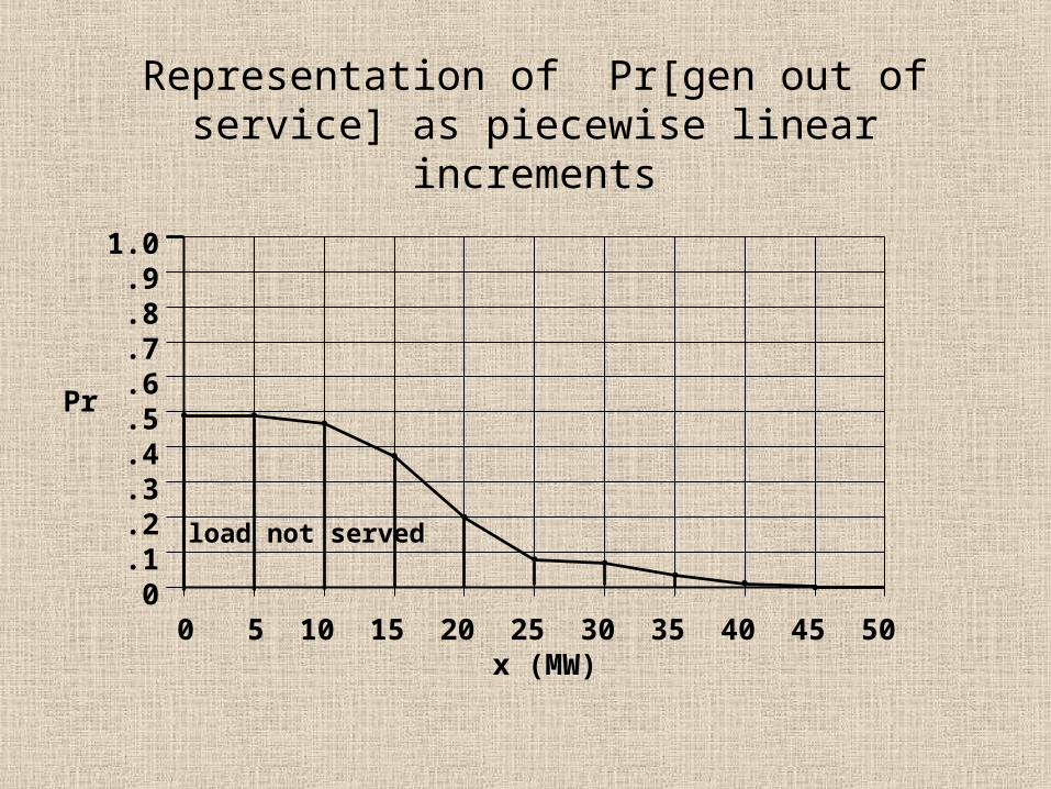
Representation of Pr[gen out of service] as piecewise linear increments
1.0 .9 .8 .7 .6 .5 .4 .3 .2 .1 0 0 5 10 15 20 25 30 35 40 45 50 x (MW)
Pr
load not served
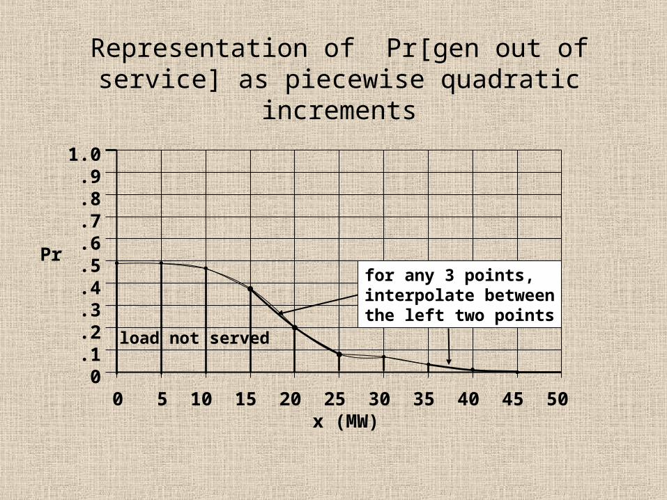
Representation of Pr[gen out of service] as piecewise quadratic increments
1.0 .9 .8 .7 .6 .5 .4 .3 .2 .1 0 0 5 10 15 20 25 30 35 40 45 50 x (MW)
Pr
load not served
for any 3 points, interpolate between the left two points
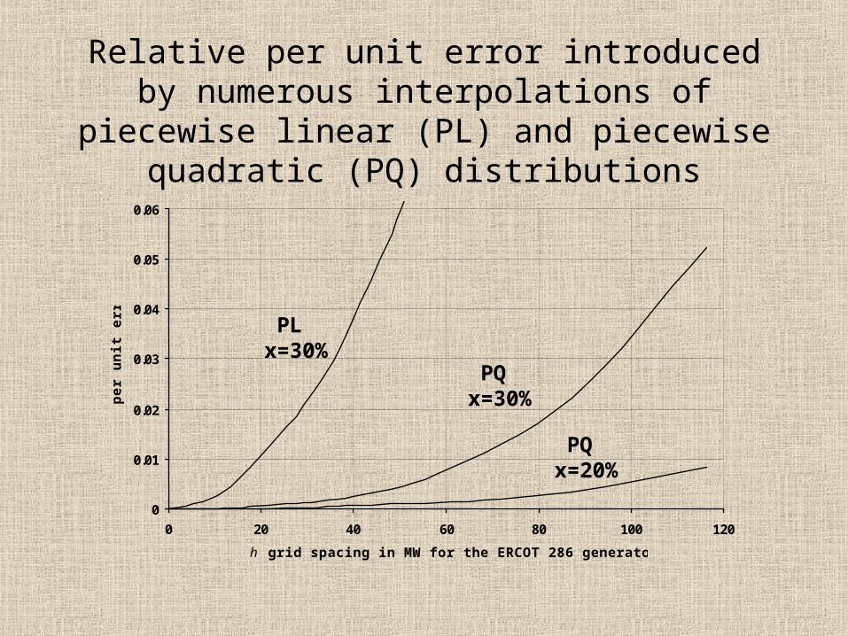
Relative per unit error introduced by numerous interpolations of piecewise linear (PL) and
piecewise quadratic (PQ) distributions
0
0.01
0.02
0.03
0.04
0.05
0.06
0 20 40 60 80 100 120
h grid spacing in MW for the ERCOT 286 generator problem
per
un
it e
rro
r PLx=30%
PQx=30%
PQx=20%
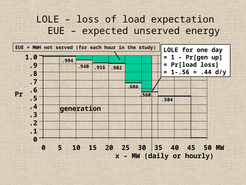
LOLE – loss of load expectation EUE – expected unserved energy
1.0 .9 .8 .7 .6 .5 .4 .3 .2 .1 0 0 5 10 15 20 25 30 35 40 45 50 MW x – MW (daily or hourly)
Pr
EUE = MWH not served (for each hour in the study)
generation
LOLE for one day= 1 - Pr[gen up]= Pr[load loss]= 1-.56 = .44 d/y
.686
.560.504
.994.940 .916 .902
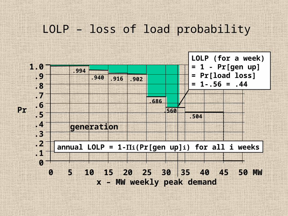
LOLP – loss of load probability
1.0 .9 .8 .7 .6 .5 .4 .3 .2 .1 0 0 5 10 15 20 25 30 35 40 45 50 MW x – MW weekly peak demand
Pr
generation
LOLP (for a week)= 1 - Pr[gen up]= Pr[load loss]= 1-.56 = .44
.686
.560.504
.994.940 .916 .902
annual LOLP = 1-i(Pr[gen up]i) for all i weeks
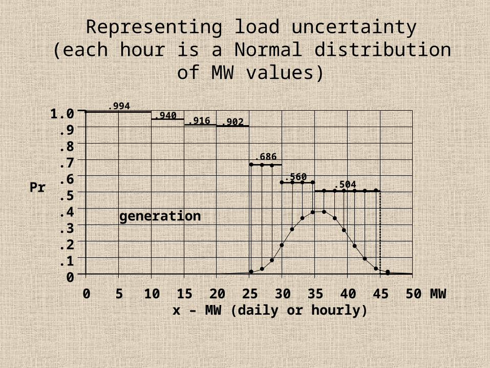
Representing load uncertainty(each hour is a Normal distribution of MW values)
1.0 .9 .8 .7 .6 .5 .4 .3 .2 .1 0 0 5 10 15 20 25 30 35 40 45 50 MW x – MW (daily or hourly)
Pr
generation
.686
.560.504
.994.940 .916 .902
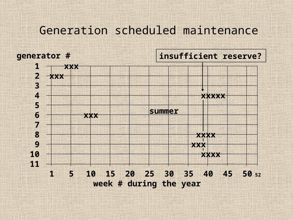
Generation scheduled maintenance
1 xxx 2 xxx 3 4 xxxxx 5 6 xxx 7 8 xxxx 9 xxx10 xxxx11 1 5 10 15 20 25 30 35 40 45 50 52 week # during the year
generator #
summer
insufficient reserve?
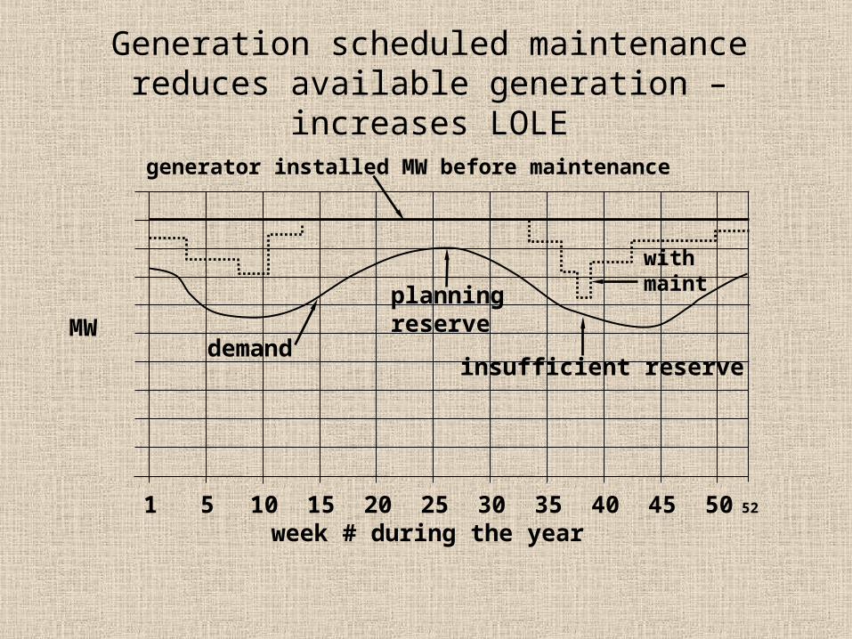
Generation scheduled maintenancereduces available generation – increases LOLE
1 5 10 15 20 25 30 35 40 45 50 52 week # during the year
generator installed MW before maintenance
MWdemand
insufficient reserve
planningreserve
withmaint
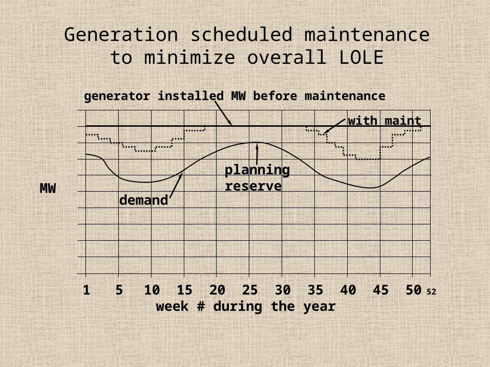
Generation scheduled maintenanceto minimize overall LOLE
1 5 10 15 20 25 30 35 40 45 50 52 week # during the year
generator installed MW before maintenance
MWdemand
planningreserve
with maint
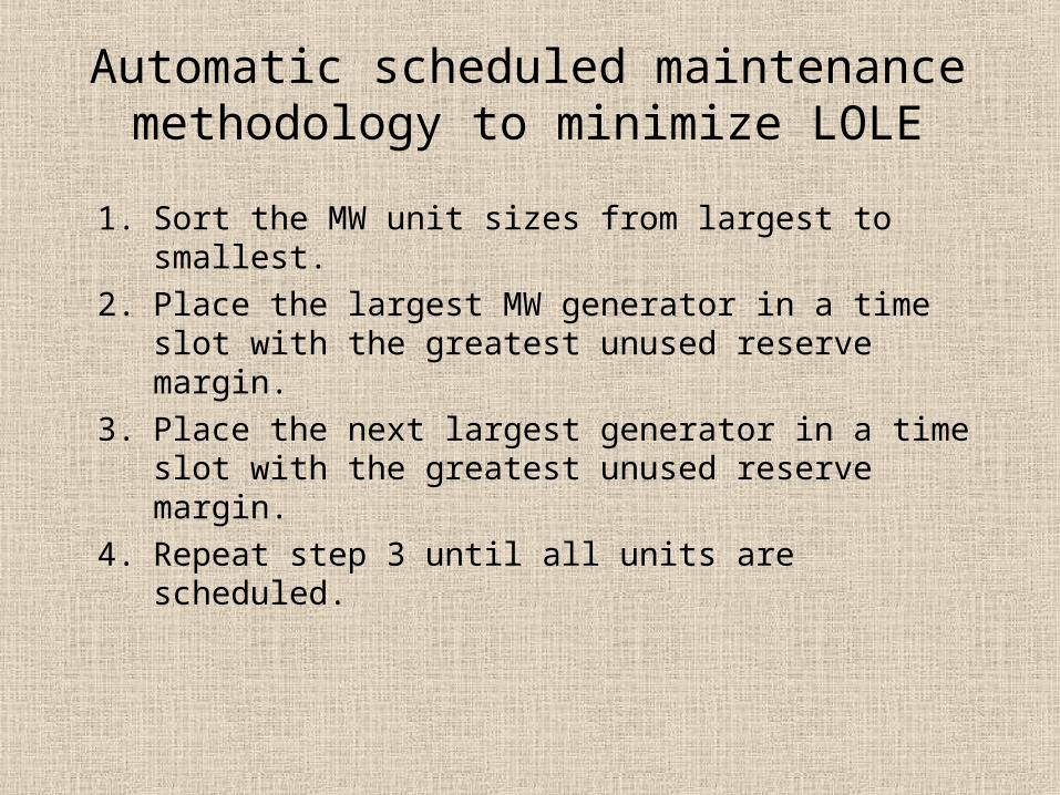
Automatic scheduled maintenance methodology to minimize LOLE
1. Sort the MW unit sizes from largest to smallest.
2. Place the largest MW generator in a time slot with the greatest unused reserve margin.
3. Place the next largest generator in a time slot with the greatest unused reserve margin.
4. Repeat step 3 until all units are scheduled.
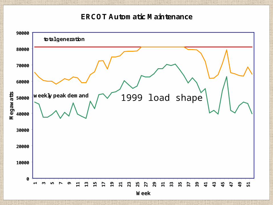
ERCOT Automatic Maintenance
0
10000
20000
30000
40000
50000
60000
70000
80000
900001 3 5 7 9
11
13
15
17
19
21
23
25
27
29
31
33
35
37
39
41
43
45
47
49
51
Week
Me
ga
wa
tts weekly peak demand
automatic maintenance
total generation
1999 load shape
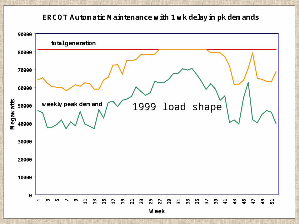
ERCOT Automatic Maintenance with 1 wk delay in pk demands
0
10000
20000
30000
40000
50000
60000
70000
80000
900001 3 5 7 9
11
13
15
17
19
21
23
25
27
29
31
33
35
37
39
41
43
45
47
49
51
Week
Me
ga
wa
tts weekly peak demand
automatic maintenance
total generation
1999 load shape
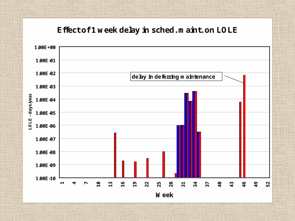
Effect of 1 week delay in sched. maint. on LOLE
1.00E-10
1.00E-09
1.00E-08
1.00E-07
1.00E-06
1.00E-05
1.00E-04
1.00E-03
1.00E-02
1.00E-01
1.00E+00
1 4 7
10
13
16
19
22
25
28
31
34
37
40
43
46
49
52
Week
LO
LE
- d
ay
s/y
ea
r
delay in deferring maintenance
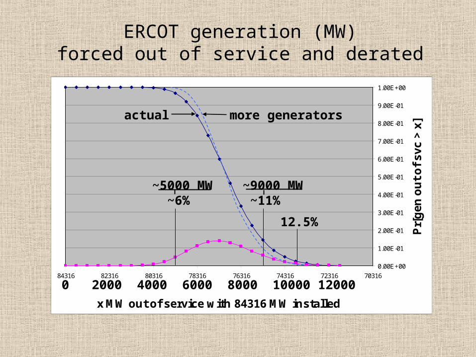
ERCOT generation (MW)forced out of service and derated
0.00E+00
1.00E-01
2.00E-01
3.00E-01
4.00E-01
5.00E-01
6.00E-01
7.00E-01
8.00E-01
9.00E-01
1.00E+00
7031672316743167631678316803168231684316
x MW out of service with 84316 MW installed
Pr[
ge
n o
ut
of
sv
c >
x]
0 2000 4000 6000 8000 10000 12000
~5000 MW ~9000 MW ~6% ~11%
12.5%
actual more generators
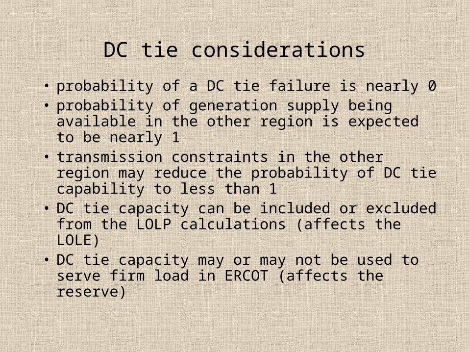
DC tie considerations
• probability of a DC tie failure is nearly 0• probability of generation supply being available
in the other region is expected to be nearly 1• transmission constraints in the other region
may reduce the probability of DC tie capability to less than 1
• DC tie capacity can be included or excluded from the LOLP calculations (affects the LOLE)
• DC tie capacity may or may not be used to serve firm load in ERCOT (affects the reserve)
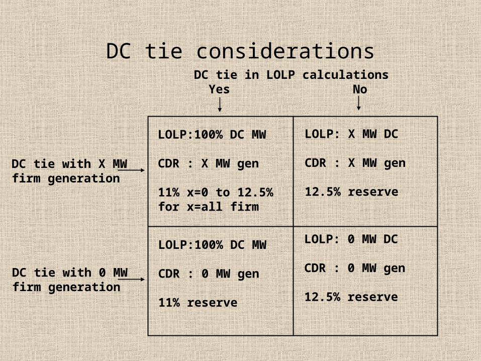
DC tie considerations
DC tie with X MWfirm generation
DC tie with 0 MWfirm generation
DC tie in LOLP calculations Yes No
LOLP:100% DC MW
CDR : X MW gen
11% x=0 to 12.5% for x=all firm
LOLP: X MW DC
CDR : X MW gen
12.5% reserve
LOLP:100% DC MW
CDR : 0 MW gen
11% reserve
LOLP: 0 MW DC
CDR : 0 MW gen
12.5% reserve
Switchable generation considerations
• Switchable generation capability must be available to ERCOT when called upon.
• The same switchable MWs must be used in both the reserve calculation and the LOLP calculation.

Self-serve generation considerations
• Currently, both the self serve generation and self serve load (840 MW in the previous study) are omitted from the CDR and the LOLP calculations.
• Alternately, the self serve generation and load could be included with the CDR and LOLP calculations with a negligible effect on LOLE.
• Currently, self serve generation and load are included in the transmission load flow analysis as fixed MW values with 100% availability.
Interruptible load considerations
• The load can be modeled as two components, firm plus interruptible (i.e. two forecasts)
• The LOLE for serving firm load can be calculated by using only the forecast for firm load in the computer simulation.
• The LOLE for interruptible load can be calculated by using a forecast of firm load plus interruptible load in the computer simulation and then subtracting the LOLE results obtained for the firm load forecast.
Data needed to perform single-area LOLP studies
• hourly ERCOT loads for the (annual) study period (historical year hourly loads are scaled)
• the annual peak demand forecast and the percentage of interruptible load
• percentage of load forecast uncertainty• each generator’s seasonal MW (Pmax)
capability, fuel type, type of unit, and maintenance periods (by beginning and ending week numbers or by total weeks needed)
• FOR and DFOR of generator types such as gas, coal, nuclear, hydro, wind, etc.
• identification of self-serve MW by generator
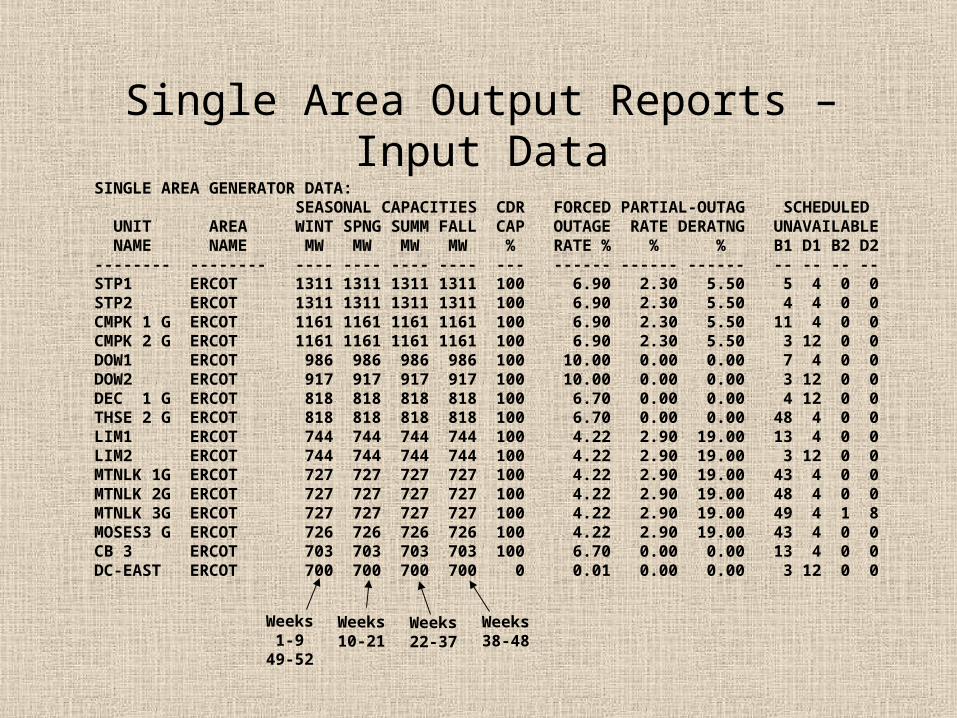
Single Area Output Reports – Input Data SINGLE AREA GENERATOR DATA: SEASONAL CAPACITIES CDR FORCED PARTIAL-OUTAG SCHEDULED UNIT AREA WINT SPNG SUMM FALL CAP OUTAGE RATE DERATNG UNAVAILABLE NAME NAME MW MW MW MW % RATE % % % B1 D1 B2 D2 -------- -------- ---- ---- ---- ---- --- ------ ------ ------ -- -- -- -- STP1 ERCOT 1311 1311 1311 1311 100 6.90 2.30 5.50 5 4 0 0 STP2 ERCOT 1311 1311 1311 1311 100 6.90 2.30 5.50 4 4 0 0 CMPK 1 G ERCOT 1161 1161 1161 1161 100 6.90 2.30 5.50 11 4 0 0 CMPK 2 G ERCOT 1161 1161 1161 1161 100 6.90 2.30 5.50 3 12 0 0 DOW1 ERCOT 986 986 986 986 100 10.00 0.00 0.00 7 4 0 0 DOW2 ERCOT 917 917 917 917 100 10.00 0.00 0.00 3 12 0 0 DEC 1 G ERCOT 818 818 818 818 100 6.70 0.00 0.00 4 12 0 0 THSE 2 G ERCOT 818 818 818 818 100 6.70 0.00 0.00 48 4 0 0 LIM1 ERCOT 744 744 744 744 100 4.22 2.90 19.00 13 4 0 0 LIM2 ERCOT 744 744 744 744 100 4.22 2.90 19.00 3 12 0 0 MTNLK 1G ERCOT 727 727 727 727 100 4.22 2.90 19.00 43 4 0 0 MTNLK 2G ERCOT 727 727 727 727 100 4.22 2.90 19.00 48 4 0 0 MTNLK 3G ERCOT 727 727 727 727 100 4.22 2.90 19.00 49 4 1 8 MOSES3 G ERCOT 726 726 726 726 100 4.22 2.90 19.00 43 4 0 0 CB 3 ERCOT 703 703 703 703 100 6.70 0.00 0.00 13 4 0 0 DC-EAST ERCOT 700 700 700 700 0 0.01 0.00 0.00 3 12 0 0
Weeks 1-949-52
Weeks10-21
Weeks22-37
Weeks38-48
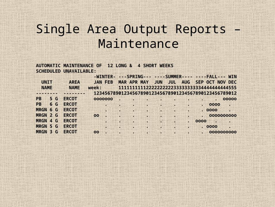
Single Area Output Reports – Maintenance
AUTOMATIC MAINTENANCE OF 12 LONG & 4 SHORT WEEKS SCHEDULED UNAVAILABLE: -WINTER- ---SPRING--- ----SUMMER---- ----FALL--- WIN UNIT AREA JAN FEB MAR APR MAY JUN JUL AUG SEP OCT NOV DEC NAME NAME week: 1111111111222222222233333333334444444444555 -------- -------- 1234567890123456789012345678901234567890123456789012 PB 5 G ERCOT ooooooo . . . . . . . . ooooo PB 6 G ERCOT . . . . . . . . oooo . MRGN 6 G ERCOT . . . . . . . . oooo . MRGN 2 G ERCOT oo . . . . . . . . oooooooooo MRGN 4 G ERCOT . . . . . . . oooo . . MRGN 5 G ERCOT . . . . . . . . oooo . MRGN 3 G ERCOT oo . . . . . . . . oooooooooo
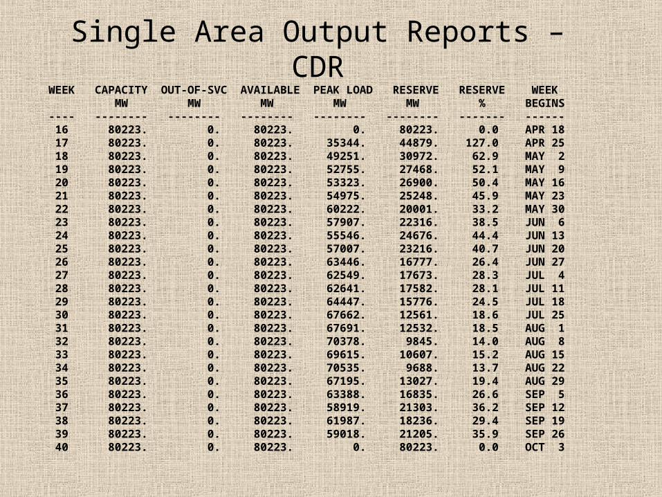
Single Area Output Reports – CDR WEEK CAPACITY OUT-OF-SVC AVAILABLE PEAK LOAD RESERVE RESERVE WEEK MW MW MW MW MW % BEGINS ---- -------- -------- -------- -------- -------- ------- ------ 16 80223. 0. 80223. 0. 80223. 0.0 APR 18 17 80223. 0. 80223. 35344. 44879. 127.0 APR 25 18 80223. 0. 80223. 49251. 30972. 62.9 MAY 2 19 80223. 0. 80223. 52755. 27468. 52.1 MAY 9 20 80223. 0. 80223. 53323. 26900. 50.4 MAY 16 21 80223. 0. 80223. 54975. 25248. 45.9 MAY 23 22 80223. 0. 80223. 60222. 20001. 33.2 MAY 30 23 80223. 0. 80223. 57907. 22316. 38.5 JUN 6 24 80223. 0. 80223. 55546. 24676. 44.4 JUN 13 25 80223. 0. 80223. 57007. 23216. 40.7 JUN 20 26 80223. 0. 80223. 63446. 16777. 26.4 JUN 27 27 80223. 0. 80223. 62549. 17673. 28.3 JUL 4 28 80223. 0. 80223. 62641. 17582. 28.1 JUL 11 29 80223. 0. 80223. 64447. 15776. 24.5 JUL 18 30 80223. 0. 80223. 67662. 12561. 18.6 JUL 25 31 80223. 0. 80223. 67691. 12532. 18.5 AUG 1 32 80223. 0. 80223. 70378. 9845. 14.0 AUG 8 33 80223. 0. 80223. 69615. 10607. 15.2 AUG 15 34 80223. 0. 80223. 70535. 9688. 13.7 AUG 22 35 80223. 0. 80223. 67195. 13027. 19.4 AUG 29 36 80223. 0. 80223. 63388. 16835. 26.6 SEP 5 37 80223. 0. 80223. 58919. 21303. 36.2 SEP 12 38 80223. 0. 80223. 61987. 18236. 29.4 SEP 19 39 80223. 0. 80223. 59018. 21205. 35.9 SEP 26 40 80223. 0. 80223. 0. 80223. 0.0 OCT 3
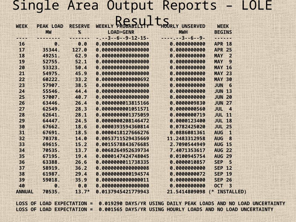
Single Area Output Reports – LOLE Results WEEK PEAK LOAD RESERVE WEEKLY PROBABILITY HOURLY UNSERVED WEEK MW % LOAD>GENR MWH BEGINS ---- -------- ------- -.--3--6--9-12-15- ----.--3--6--9- ------ 16 0. 0.0 0.0000000000000000 0.0000000000 APR 18 17 35344. 127.0 0.0000000000000000 0.0000000000 APR 25 18 49251. 62.9 0.0000000000000000 0.0000000000 MAY 2 19 52755. 52.1 0.0000000000000000 0.0000000000 MAY 9 20 53323. 50.4 0.0000000000000000 0.0000000000 MAY 16 21 54975. 45.9 0.0000000000000000 0.0000000000 MAY 23 22 60222. 33.2 0.0000000000000692 0.0000000000 MAY 30 23 57907. 38.5 0.0000000000000000 0.0000000000 JUN 6 24 55546. 44.4 0.0000000000000000 0.0000000000 JUN 13 25 57007. 40.7 0.0000000000000000 0.0000000000 JUN 20 26 63446. 26.4 0.0000000013815166 0.0000009830 JUN 27 27 62549. 28.3 0.0000000001051571 0.0000000560 JUL 4 28 62641. 28.1 0.0000000001375059 0.0000000719 JUL 11 29 64447. 24.5 0.0000000208146472 0.0000123400 JUL 18 30 67662. 18.6 0.0000393594360814 0.0782425020 JUL 25 31 67691. 18.5 0.0000418127666276 0.0886081361 AUG 1 32 70378. 14.0 0.0053711529435669 11.2483312958 AUG 8 33 69615. 15.2 0.0015578843676685 2.7090544949 AUG 15 34 70535. 13.7 0.0068264952639734 7.4071353617 AUG 22 35 67195. 19.4 0.0000147424748045 0.0100945754 AUG 29 36 63388. 26.6 0.0000000011738335 0.0000010857 SEP 5 37 58919. 36.2 0.0000000000000008 0.0000000000 SEP 12 38 61987. 29.4 0.0000000000194574 0.0000000072 SEP 19 39 59018. 35.9 0.0000000000000011 0.0000000000 SEP 26 40 0. 0.0 0.0000000000000000 0.0000000000 OCT 3 ANNUAL 70535. 13.7* 0.0137945421779943 21.5414809098 (* INSTALLED)
LOSS OF LOAD EXPECTATION = 0.019290 DAYS/YR USING DAILY PEAK LOADS AND NO LOAD UNCERTAINTY LOSS OF LOAD EXPECTATION = 0.001565 DAYS/YR USING HOURLY LOADS AND NO LOAD UNCERTAINTY
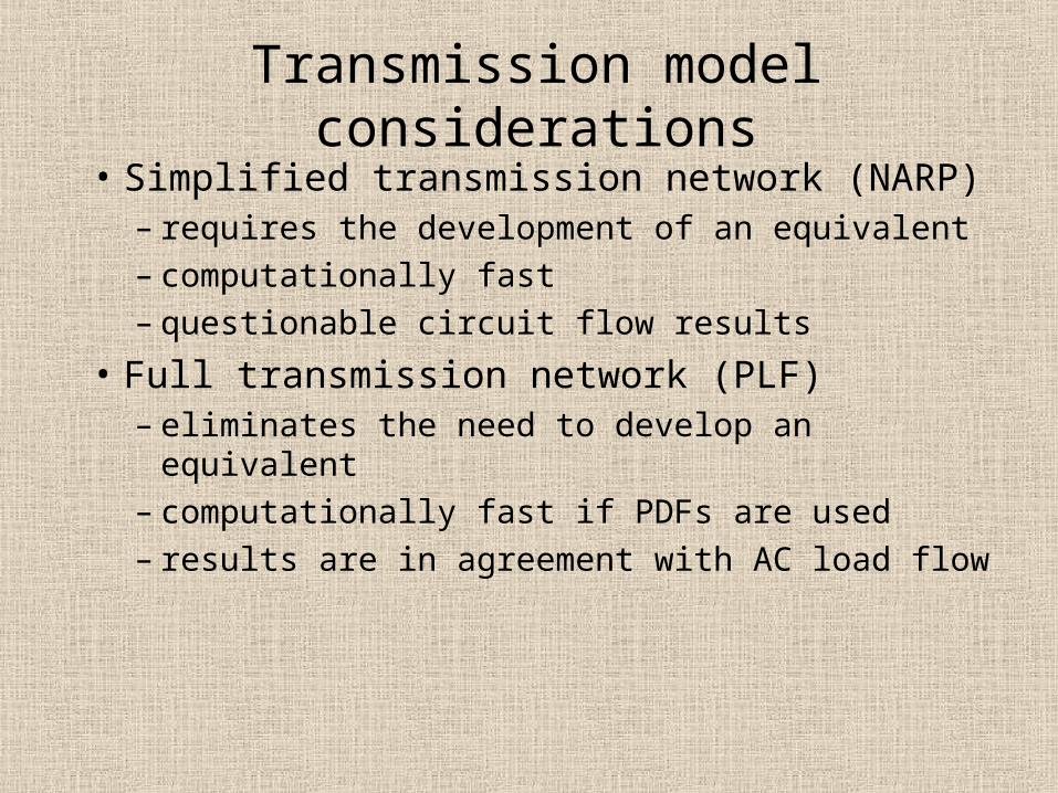
Transmission model considerations
• Simplified transmission network (NARP)– requires the development of an equivalent– computationally fast– questionable circuit flow results
• Full transmission network (PLF)– eliminates the need to develop an equivalent– computationally fast if PDFs are used– results are in agreement with AC load flow
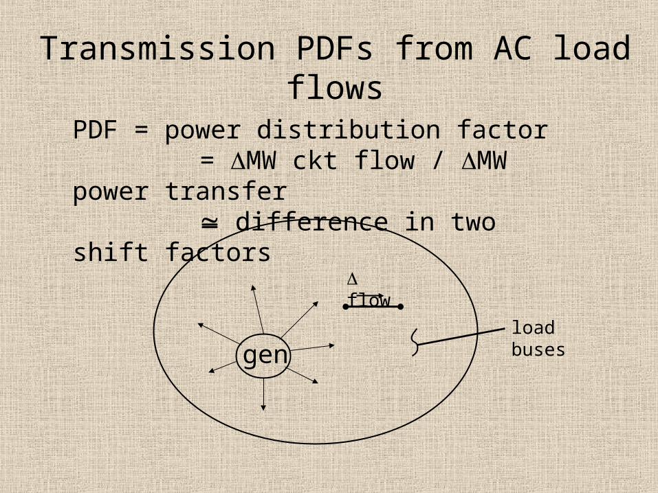
Transmission PDFs from AC load flows
PDF = power distribution factor = MW ckt flow / MW power transfer difference in two shift factors
gen
flow
load buses
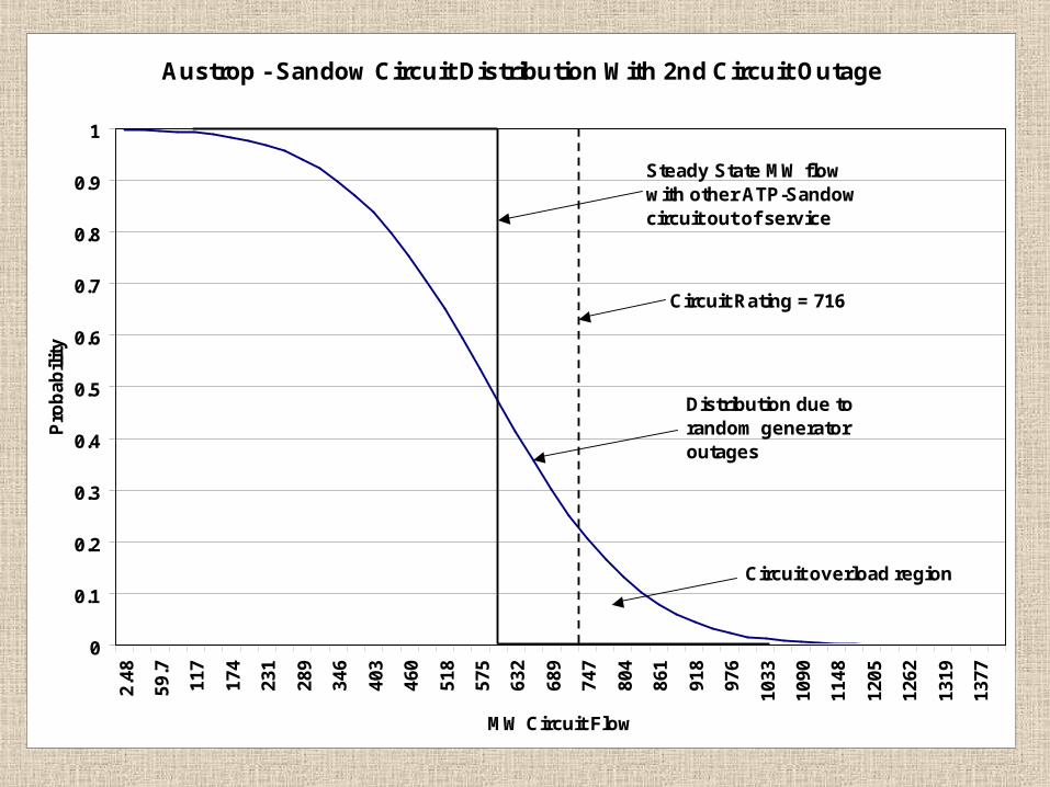
Austrop - Sandow Circuit Distribution With 2nd Circuit Outage
0
0.1
0.2
0.3
0.4
0.5
0.6
0.7
0.8
0.9
12.
48
59.7
117
174
231
289
346
403
460
518
575
632
689
747
804
861
918
976
1033
1090
1148
1205
1262
1319
1377
MW Circuit Flow
Pro
bab
ility
Steady State MW flow with other ATP-Sandow circuit out of service
Circuit Rating = 716
Distribution due to random generator outages
Circuit overload region
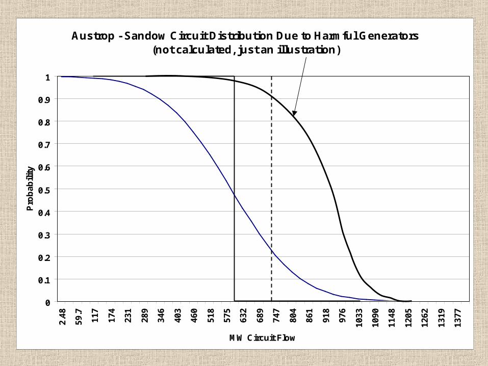
Austrop - Sandow Circuit Distribution Due to Harmful Generators(not calculated, just an illustration)
0
0.1
0.2
0.3
0.4
0.5
0.6
0.7
0.8
0.9
1
2.48
59.7
117
174
231
289
346
403
460
518
575
632
689
747
804
861
918
976
1033
1090
1148
1205
1262
1319
1377
MW Circuit Flow
Pro
bab
ility
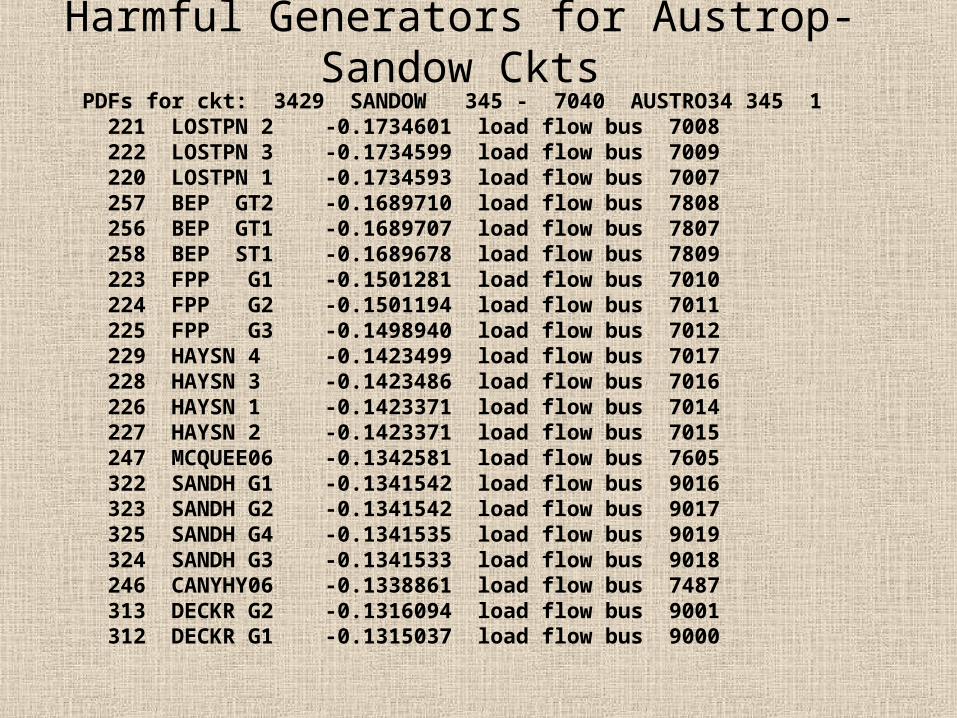
Harmful Generators for Austrop-Sandow Ckts
PDFs for ckt: 3429 SANDOW 345 - 7040 AUSTRO34 345 1 221 LOSTPN 2 -0.1734601 load flow bus 7008 222 LOSTPN 3 -0.1734599 load flow bus 7009 220 LOSTPN 1 -0.1734593 load flow bus 7007 257 BEP GT2 -0.1689710 load flow bus 7808 256 BEP GT1 -0.1689707 load flow bus 7807 258 BEP ST1 -0.1689678 load flow bus 7809 223 FPP G1 -0.1501281 load flow bus 7010 224 FPP G2 -0.1501194 load flow bus 7011 225 FPP G3 -0.1498940 load flow bus 7012 229 HAYSN 4 -0.1423499 load flow bus 7017 228 HAYSN 3 -0.1423486 load flow bus 7016 226 HAYSN 1 -0.1423371 load flow bus 7014 227 HAYSN 2 -0.1423371 load flow bus 7015 247 MCQUEE06 -0.1342581 load flow bus 7605 322 SANDH G1 -0.1341542 load flow bus 9016 323 SANDH G2 -0.1341542 load flow bus 9017 325 SANDH G4 -0.1341535 load flow bus 9019 324 SANDH G3 -0.1341533 load flow bus 9018 246 CANYHY06 -0.1338861 load flow bus 7487 313 DECKR G2 -0.1316094 load flow bus 9001 312 DECKR G1 -0.1315037 load flow bus 9000
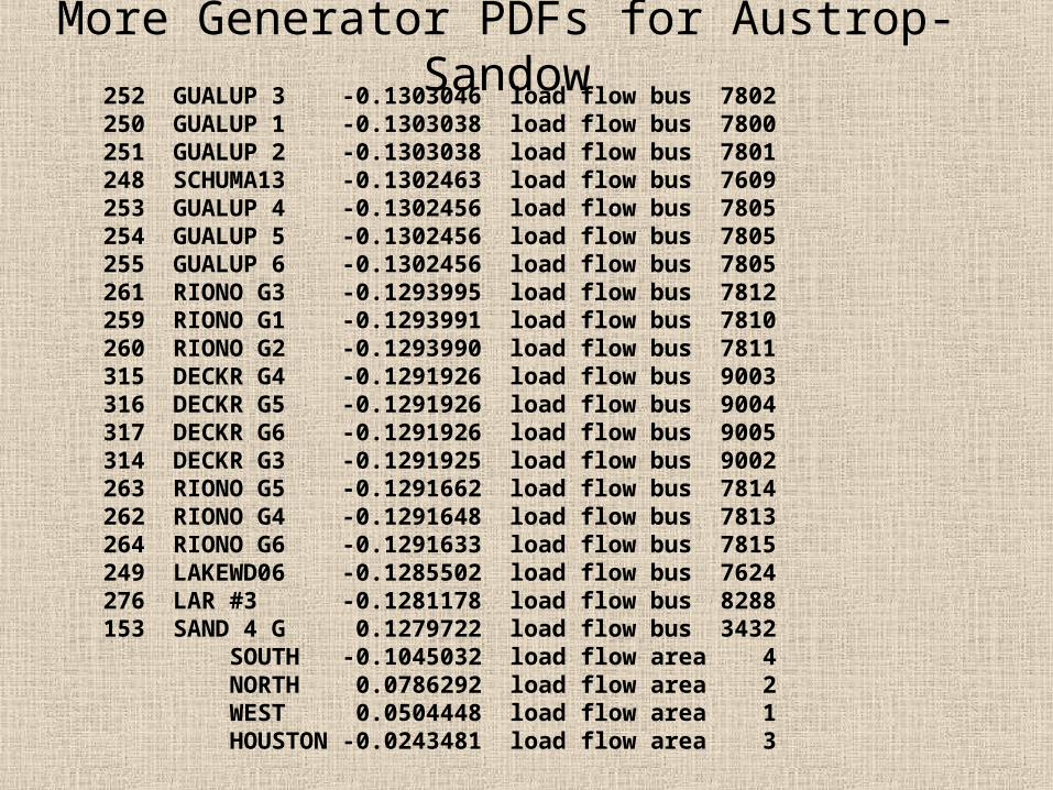
More Generator PDFs for Austrop-Sandow 252 GUALUP 3 -0.1303046 load flow bus 7802 250 GUALUP 1 -0.1303038 load flow bus 7800 251 GUALUP 2 -0.1303038 load flow bus 7801 248 SCHUMA13 -0.1302463 load flow bus 7609 253 GUALUP 4 -0.1302456 load flow bus 7805 254 GUALUP 5 -0.1302456 load flow bus 7805 255 GUALUP 6 -0.1302456 load flow bus 7805 261 RIONO G3 -0.1293995 load flow bus 7812 259 RIONO G1 -0.1293991 load flow bus 7810 260 RIONO G2 -0.1293990 load flow bus 7811 315 DECKR G4 -0.1291926 load flow bus 9003 316 DECKR G5 -0.1291926 load flow bus 9004 317 DECKR G6 -0.1291926 load flow bus 9005 314 DECKR G3 -0.1291925 load flow bus 9002 263 RIONO G5 -0.1291662 load flow bus 7814 262 RIONO G4 -0.1291648 load flow bus 7813 264 RIONO G6 -0.1291633 load flow bus 7815 249 LAKEWD06 -0.1285502 load flow bus 7624 276 LAR #3 -0.1281178 load flow bus 8288 153 SAND 4 G 0.1279722 load flow bus 3432 SOUTH -0.1045032 load flow area 4 NORTH 0.0786292 load flow area 2 WEST 0.0504448 load flow area 1 HOUSTON -0.0243481 load flow area 3
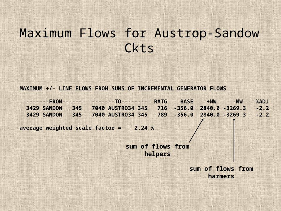
Maximum Flows for Austrop-Sandow Ckts
MAXIMUM +/- LINE FLOWS FROM SUMS OF INCREMENTAL GENERATOR FLOWS
-------FROM------ -------TO-------- RATG BASE +MW -MW %ADJ 3429 SANDOW 345 7040 AUSTRO34 345 716 -356.0 2840.0 -3269.3 -2.2 3429 SANDOW 345 7040 AUSTRO34 345 789 -356.0 2840.0 -3269.3 -2.2
average weighted scale factor = 2.24 %
sum of flows from helpers
sum of flows from harmers
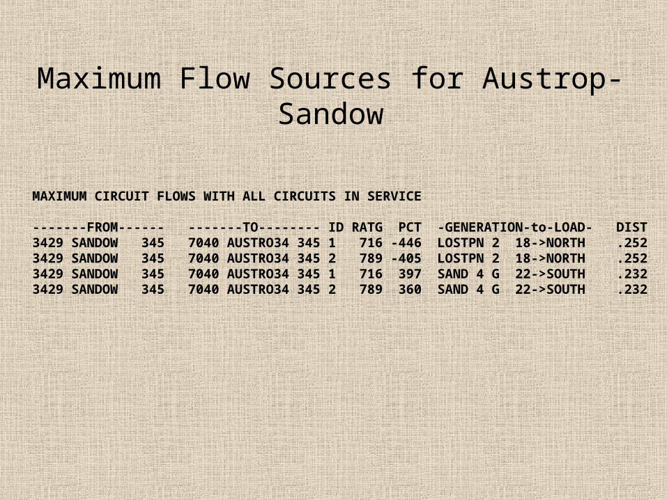
Maximum Flow Sources for Austrop-Sandow
MAXIMUM CIRCUIT FLOWS WITH ALL CIRCUITS IN SERVICE
-------FROM------ -------TO-------- ID RATG PCT -GENERATION-to-LOAD- DIST 3429 SANDOW 345 7040 AUSTRO34 345 1 716 -446 LOSTPN 2 18->NORTH .252 3429 SANDOW 345 7040 AUSTRO34 345 2 789 -405 LOSTPN 2 18->NORTH .252 3429 SANDOW 345 7040 AUSTRO34 345 1 716 397 SAND 4 G 22->SOUTH .232 3429 SANDOW 345 7040 AUSTRO34 345 2 789 360 SAND 4 G 22->SOUTH .232
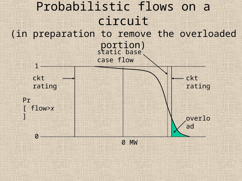
0 MW
Pr [ flow>x ]
0
1
ckt rating ckt rating
static base case flow
overload
Probabilistic flows on a circuit(in preparation to remove the overloaded portion)
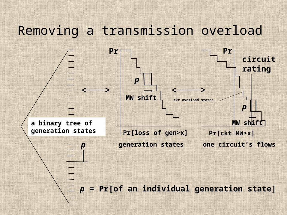
Removing a transmission overload
ckt overload states
p
p
p
PrPr
Pr[loss of gen>x] Pr[ckt MW>x]
p = Pr[of an individual generation state]
generation states one circuit’s flows
MW shift
MW shifta binary tree of generation states
circuit rating
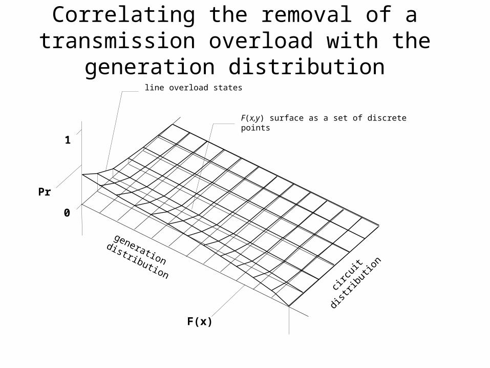
Correlating the removal of a transmission overload with the generation distribution
line overload states
F(x,y) surface as a set of discrete points
1
0
Pr
F(x)
generation distribution
circu
it di
strib
ution
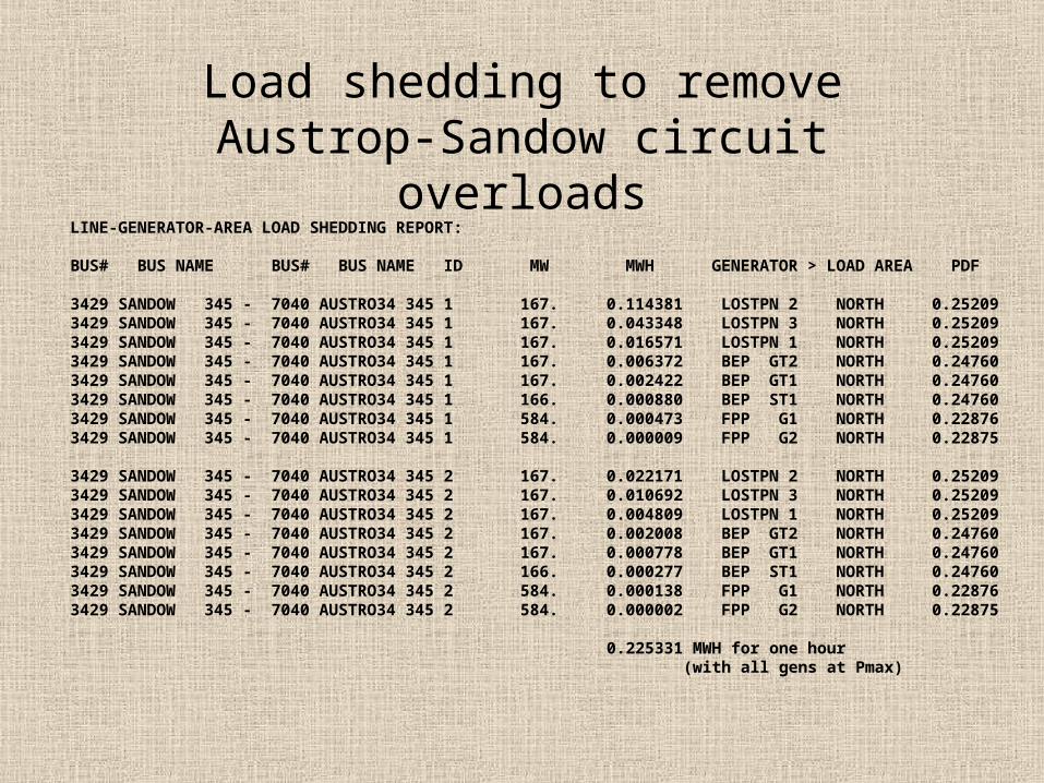
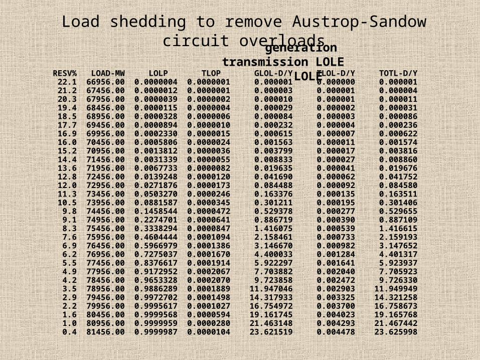
Load shedding to remove Austrop-Sandow circuit overloads
LINE-GENERATOR-AREA LOAD SHEDDING REPORT:
BUS# BUS NAME BUS# BUS NAME ID MW MWH GENERATOR > LOAD AREA PDF 3429 SANDOW 345 - 7040 AUSTRO34 345 1 167. 0.114381 LOSTPN 2 NORTH 0.25209 3429 SANDOW 345 - 7040 AUSTRO34 345 1 167. 0.043348 LOSTPN 3 NORTH 0.25209 3429 SANDOW 345 - 7040 AUSTRO34 345 1 167. 0.016571 LOSTPN 1 NORTH 0.25209 3429 SANDOW 345 - 7040 AUSTRO34 345 1 167. 0.006372 BEP GT2 NORTH 0.24760 3429 SANDOW 345 - 7040 AUSTRO34 345 1 167. 0.002422 BEP GT1 NORTH 0.24760 3429 SANDOW 345 - 7040 AUSTRO34 345 1 166. 0.000880 BEP ST1 NORTH 0.24760 3429 SANDOW 345 - 7040 AUSTRO34 345 1 584. 0.000473 FPP G1 NORTH 0.22876 3429 SANDOW 345 - 7040 AUSTRO34 345 1 584. 0.000009 FPP G2 NORTH 0.22875 3429 SANDOW 345 - 7040 AUSTRO34 345 2 167. 0.022171 LOSTPN 2 NORTH 0.25209 3429 SANDOW 345 - 7040 AUSTRO34 345 2 167. 0.010692 LOSTPN 3 NORTH 0.25209 3429 SANDOW 345 - 7040 AUSTRO34 345 2 167. 0.004809 LOSTPN 1 NORTH 0.25209 3429 SANDOW 345 - 7040 AUSTRO34 345 2 167. 0.002008 BEP GT2 NORTH 0.24760 3429 SANDOW 345 - 7040 AUSTRO34 345 2 167. 0.000778 BEP GT1 NORTH 0.24760 3429 SANDOW 345 - 7040 AUSTRO34 345 2 166. 0.000277 BEP ST1 NORTH 0.24760 3429 SANDOW 345 - 7040 AUSTRO34 345 2 584. 0.000138 FPP G1 NORTH 0.22876 3429 SANDOW 345 - 7040 AUSTRO34 345 2 584. 0.000002 FPP G2 NORTH 0.22875
0.225331 MWH for one hour (with all gens at Pmax)
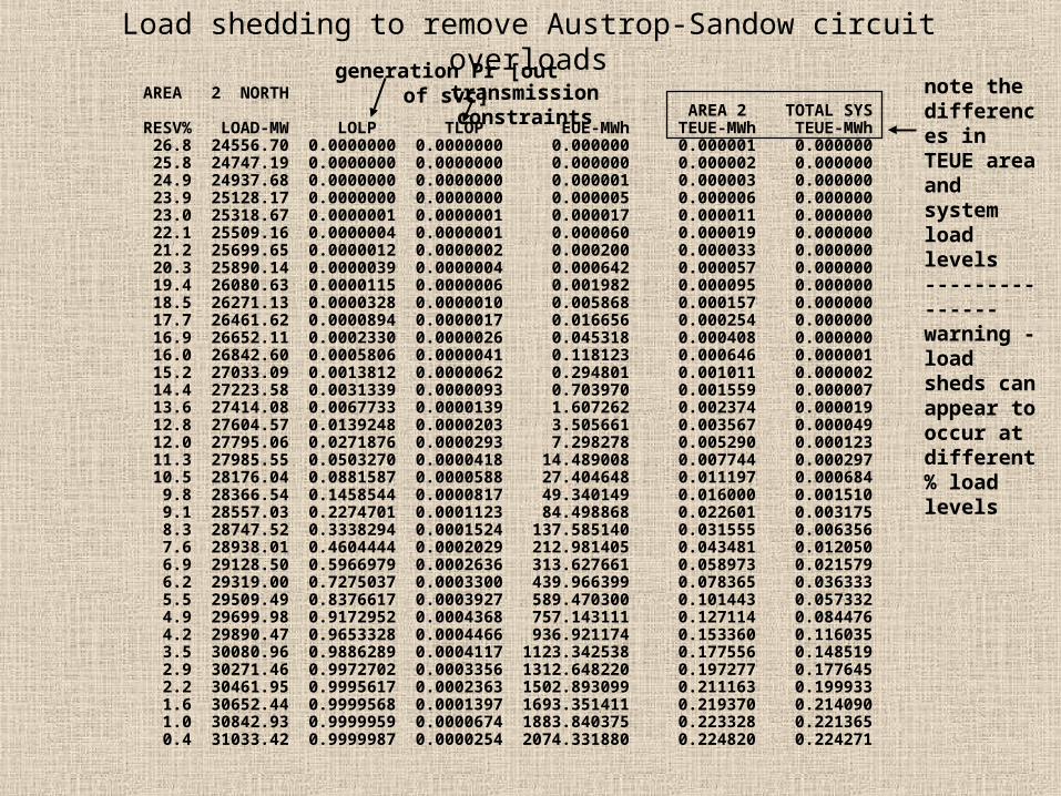
Load shedding to remove Austrop-Sandow circuit overloads
AREA 2 NORTH AREA 2 TOTAL SYS RESV% LOAD-MW LOLP TLOP EUE-MWh TEUE-MWh TEUE-MWh 26.8 24556.70 0.0000000 0.0000000 0.000000 0.000001 0.000000 25.8 24747.19 0.0000000 0.0000000 0.000000 0.000002 0.000000 24.9 24937.68 0.0000000 0.0000000 0.000001 0.000003 0.000000 23.9 25128.17 0.0000000 0.0000000 0.000005 0.000006 0.000000 23.0 25318.67 0.0000001 0.0000001 0.000017 0.000011 0.000000 22.1 25509.16 0.0000004 0.0000001 0.000060 0.000019 0.000000 21.2 25699.65 0.0000012 0.0000002 0.000200 0.000033 0.000000 20.3 25890.14 0.0000039 0.0000004 0.000642 0.000057 0.000000 19.4 26080.63 0.0000115 0.0000006 0.001982 0.000095 0.000000 18.5 26271.13 0.0000328 0.0000010 0.005868 0.000157 0.000000 17.7 26461.62 0.0000894 0.0000017 0.016656 0.000254 0.000000 16.9 26652.11 0.0002330 0.0000026 0.045318 0.000408 0.000000 16.0 26842.60 0.0005806 0.0000041 0.118123 0.000646 0.000001 15.2 27033.09 0.0013812 0.0000062 0.294801 0.001011 0.000002 14.4 27223.58 0.0031339 0.0000093 0.703970 0.001559 0.000007 13.6 27414.08 0.0067733 0.0000139 1.607262 0.002374 0.000019 12.8 27604.57 0.0139248 0.0000203 3.505661 0.003567 0.000049 12.0 27795.06 0.0271876 0.0000293 7.298278 0.005290 0.000123 11.3 27985.55 0.0503270 0.0000418 14.489008 0.007744 0.000297 10.5 28176.04 0.0881587 0.0000588 27.404648 0.011197 0.000684 9.8 28366.54 0.1458544 0.0000817 49.340149 0.016000 0.001510 9.1 28557.03 0.2274701 0.0001123 84.498868 0.022601 0.003175 8.3 28747.52 0.3338294 0.0001524 137.585140 0.031555 0.006356 7.6 28938.01 0.4604444 0.0002029 212.981405 0.043481 0.012050 6.9 29128.50 0.5966979 0.0002636 313.627661 0.058973 0.021579 6.2 29319.00 0.7275037 0.0003300 439.966399 0.078365 0.036333 5.5 29509.49 0.8376617 0.0003927 589.470300 0.101443 0.057332 4.9 29699.98 0.9172952 0.0004368 757.143111 0.127114 0.084476 4.2 29890.47 0.9653328 0.0004466 936.921174 0.153360 0.116035 3.5 30080.96 0.9886289 0.0004117 1123.342538 0.177556 0.148519 2.9 30271.46 0.9972702 0.0003356 1312.648220 0.197277 0.177645 2.2 30461.95 0.9995617 0.0002363 1502.893099 0.211163 0.199933 1.6 30652.44 0.9999568 0.0001397 1693.351411 0.219370 0.214090 1.0 30842.93 0.9999959 0.0000674 1883.840375 0.223328 0.221365 0.4 31033.42 0.9999987 0.0000254 2074.331880 0.224820 0.224271
note the differences in TEUE area and system load levels ---------------warning -load sheds can appear to occur at different % load levels
generation Pr [out of svc]transmission constraints
Load shedding to remove Austrop-Sandow circuit overloads
RESV% LOAD-MW LOLP TLOP GLOL-D/Y TLOL-D/Y TOTL-D/Y 22.1 66956.00 0.0000004 0.0000001 0.000001 0.000000 0.000001 21.2 67456.00 0.0000012 0.0000001 0.000003 0.000001 0.000004 20.3 67956.00 0.0000039 0.0000002 0.000010 0.000001 0.000011 19.4 68456.00 0.0000115 0.0000004 0.000029 0.000002 0.000031 18.5 68956.00 0.0000328 0.0000006 0.000084 0.000003 0.000086 17.7 69456.00 0.0000894 0.0000010 0.000232 0.000004 0.000236 16.9 69956.00 0.0002330 0.0000015 0.000615 0.000007 0.000622 16.0 70456.00 0.0005806 0.0000024 0.001563 0.000011 0.001574 15.2 70956.00 0.0013812 0.0000036 0.003799 0.000017 0.003816 14.4 71456.00 0.0031339 0.0000055 0.008833 0.000027 0.008860 13.6 71956.00 0.0067733 0.0000082 0.019635 0.000041 0.019676 12.8 72456.00 0.0139248 0.0000120 0.041690 0.000062 0.041752 12.0 72956.00 0.0271876 0.0000173 0.084488 0.000092 0.084580 11.3 73456.00 0.0503270 0.0000246 0.163376 0.000135 0.163511 10.5 73956.00 0.0881587 0.0000345 0.301211 0.000195 0.301406 9.8 74456.00 0.1458544 0.0000472 0.529378 0.000277 0.529655 9.1 74956.00 0.2274701 0.0000641 0.886719 0.000390 0.887109 8.3 75456.00 0.3338294 0.0000847 1.416075 0.000539 1.416615 7.6 75956.00 0.4604444 0.0001094 2.158461 0.000733 2.159193 6.9 76456.00 0.5966979 0.0001386 3.146670 0.000982 3.147652 6.2 76956.00 0.7275037 0.0001670 4.400033 0.001284 4.401317 5.5 77456.00 0.8376617 0.0001914 5.922297 0.001641 5.923937 4.9 77956.00 0.9172952 0.0002067 7.703882 0.002040 7.705923 4.2 78456.00 0.9653328 0.0002070 9.723858 0.002472 9.726330 3.5 78956.00 0.9886289 0.0001889 11.947046 0.002903 11.949949 2.9 79456.00 0.9972702 0.0001498 14.317933 0.003325 14.321258 2.2 79956.00 0.9995617 0.0001027 16.754972 0.003700 16.758673 1.6 80456.00 0.9999568 0.0000594 19.161745 0.004023 19.165768 1.0 80956.00 0.9999959 0.0000280 21.463148 0.004293 21.467442 0.4 81456.00 0.9999987 0.0000104 23.621519 0.004478 23.625998
generation transmission LOLE LOLE
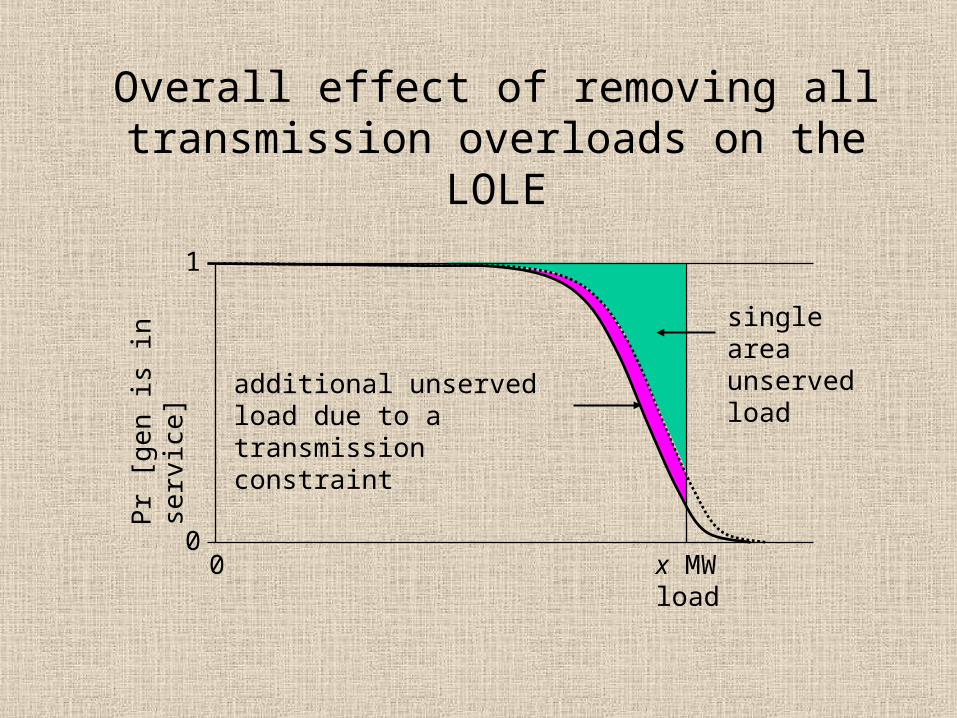
Overall effect of removing all transmission overloads on the LOLE
single area unserved load
00
1
x MW load
additional unserved load due to a transmission constraint
Pr
[ge
n is
in s
erv
ice]
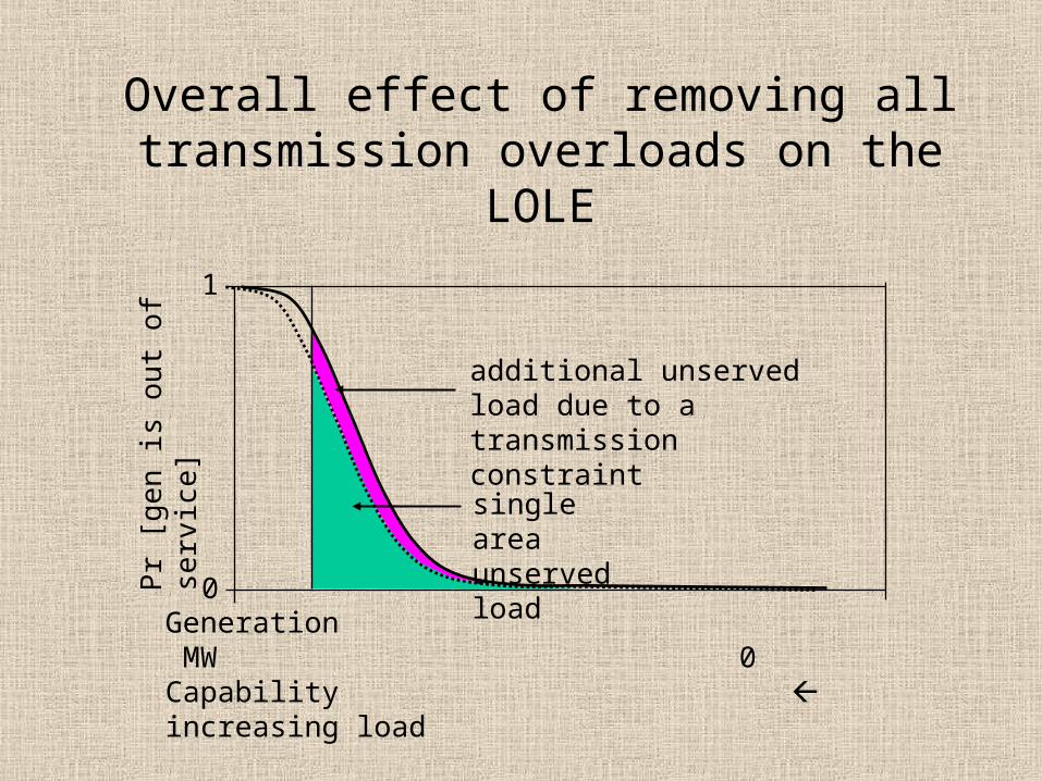
Overall effect of removing all transmission overloads on the LOLE
Pr
[ge
n is
ou
t of s
erv
ice
]
0
1
Generation MW 0Capability increasing load
single area unserved load
additional unserved load due to a transmission constraint
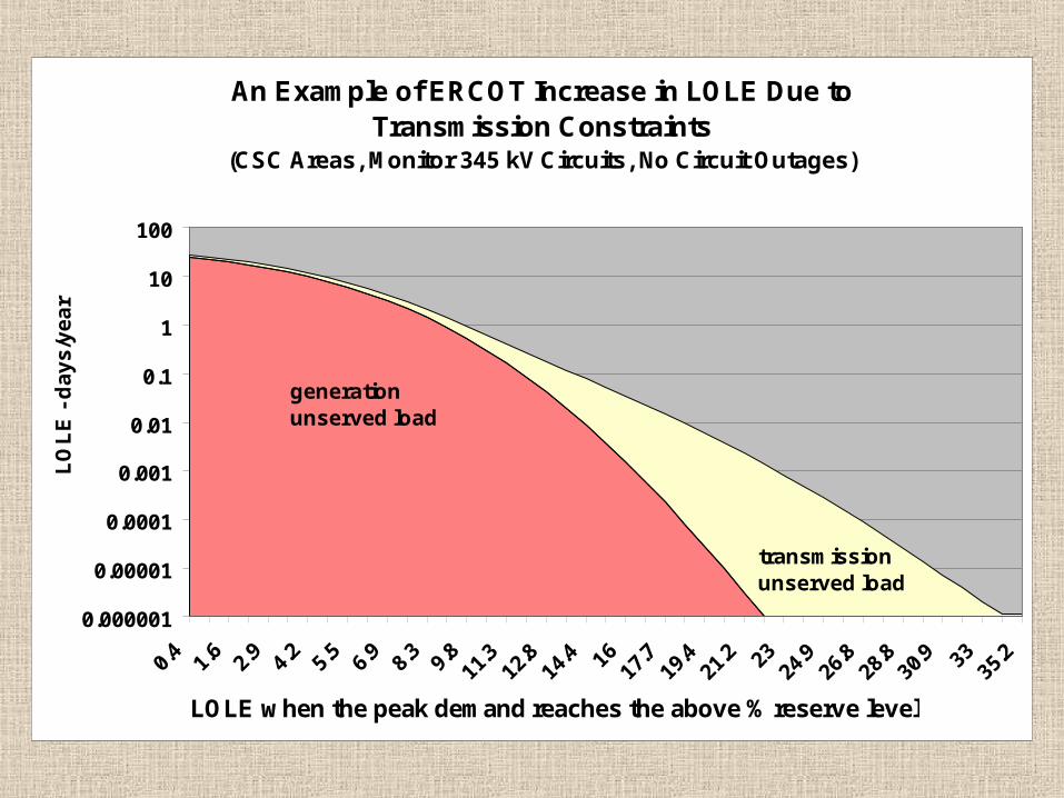
An Example of ERCOT Increase in LOLE Due to Transmission Constraints
(CSC Areas, Monitor 345 kV Circuits, No Circuit Outages)
0.000001
0.00001
0.0001
0.001
0.01
0.1
1
10
100
35.233
30.9
28.8
26.8
24.923
21.2
19.4
17.716
14.4
12.8
11.39.
88.
36.
95.
54.
22.
91.
60.
4
LOLE when the peak demand reaches the above % reserve level
LO
LE
- d
ay
s/y
ea
r
generation unserved load
transmission unserved load

See my dissertation on egpreston.com for more details.
The End