Oxford Robotics Research Group Seminar, 14 September 2007, Oxford, U.K. 1

Fundamental Matrix Computation: Theory and Practice

Kenichi Kanatani† and Yasuyuki Sugaya‡† Department of Computer Science, Okayama University, Okayama, Japan 700-8530

[email protected]‡ Department of Information and Computer Sciences, Toyohashi University of Technology,

Toyohashi, Aichi 441-8580 [email protected]

AbstractWe classify and review existing algorithms for computingthe fundamental matrix from point correspondences andpropose new effective schemes: 7-parameter Levenberg-Marquardt (LM) search, extended FNS, and EFNS-basedbundle adjustment. Doing experimental comparison, weshow that EFNS and the 7-parameter LM search exhibitthe best performance and that additional bundle adjustmentdoes not increase the accuracy to any noticeable degree.

1. Introduction

Computing the fundamental matrix from point corre-spondences is the first step of many vision applications in-cluding camera calibration, image rectification, structurefrom motion, and new view generation [7]. This problemhas attracted a special attention because of the followingtwo characteristics:

1. Feature points are extracted by an image processingoperation [8, 15, 18, 21]. As s result, the detected lo-cations invariably have uncertainty to some degree.

2. Detected points are matched by comparing surround-ing regions in respective images, using various mea-sures of similarity and correlation [13, 17, 24]. Hence,mismatches are unavoidable to some degree.

The first problem has been dealt with by statistical opti-mization [9]: we model the uncertainty as “noise” obeyinga certain probability distribution and compute a fundamen-tal matrix such that its deviation from the true value is assmall as possible in expectation. The second problem hasbeen coped with by robust estimation [19], which can beviewed as hypothesis testing: we compute a tentative fun-damental matrix as a hypothesis and check how many pointssupport it. Those points regarded as “abnormal” accordingto the hypothesis are called outliers, otherwise inliers, andwe look for a fundamental matrix that has as many inliersas possible.

Thus, the two problems are inseparably interwoven. Inthis paper, we focus on the first problem, assuming that all

corresponding points are inliers. Such a study is indispens-able for any robust estimation technique to work success-fully.

However, there is an additional compounding elementin doing statistical optimization of the fundamental ma-trix: it is constrained to have rank 2, i.e., its determinantis 0. This rank constraint has been incorporated in variousways. Here, we categorize them into the following threeapproaches:

A posteriori correction. The fundamental matrix is opti-mally computed without considering the rank con-straint and is modified in an optimal manner so thatthe constraint is satisfied (Fig. 1(a)).

Internal access. The fundamental matrix is minimally pa-rameterized so that the rank constraint is identicallysatisfied and is optimized in the reduced (“internal”)parameter space (Fig. 1(b)).

External access. We do iterations in the redundant (“ex-ternal”) parameter space in such a way that an optimalsolution that satisfies the rank constraint automaticallyresults (Fig. 1(c)).

The purpose of this paper is to review existing methodsin this framework and propose new improved methods. Inparticular, this paper contains the following three techni-cally new results:

1. We present a new internal access method 1.2. We present a new external access method 2.3. We present a new bundle adjustment algorithm3.

Then, we experimentally compare their performance, usingsimulated and real images.

In Sect. 2, we summarize the mathematical background.In Sect. 3, we study the a posteriori correction approach.We review two correction schemes (SVD correction andoptimal correction), three unconstrained optimization tech-niques (FNS, HEIV, projective Gauss-Newton iterations),

1A preliminary version was presented in our conference paper [22].2A preliminary version was presented in our conference paper [12].3This has not been presented anywhere else.

det F = 0SVD correctionoptimal correction

det F = 0 det F = 0

(a) (b) (c)

Figure 1. (a) A posteriori correction. (b) Internal access. (c) External access.

and two initialization methods (least squares (LS) and theTaubin method).

In Sect. 4, we focus on the internal access approachand present a new compact scheme for doing 7-parameterLevenberg-Marquardt (LM) search. In Sect. 5, we inves-tigate the external access approach and point out that theCFNS of Chojnacki et al. [4], a pioneering external accessmethod, does not necessarily converge to a correct solu-tion. To complement this, we present a new method, calledEFNS, and demonstrate that it always converges to an op-timal value; a mathematical justification is given to this. InSect. 6, we compare the accuracy of all the methods andconclude that our EFNS and the 7-parameter LM searchstarted from optimally corrected ML exhibit the best per-formance.

In Sect. 7, we study the bundle adjustment (Gold Stan-dard) approach and present a new efficient computationalscheme for it. In Sect. 8, we experimentally test the ef-fect of this approach and conclude that additional bundleadjustment does not increase the accuracy to any noticeabledegree. Sect. 9 concludes this paper.

2. Mathematical Fundamentals

Fundamental matrix. We are given two images of thesame scene. We take the image origin (0, 0) is at the framecenter. Suppose a point (x, y) in the first image and the cor-responding point (x′, y′) in the second. We represent themby 3-D vectors

x =

x/f0

y/f0

1

, x′ =

x′/f0

y′/f0

1

, (1)

where f0 is a scaling constant of the order of the imagesize4. Then, the following the epipolar equation is satisfied[7]:

(x, Fx′) = 0, (2)

where and throughout this paper we denote the inner prod-uct of vectors a and b by (a, b). The matrix F = (Fij)

4This is for stabilizing numerical computation [6]. In our experiments,we set f0 = 600 pixels.

in Eq. (2) is of rank 2 and called the fundamental matrix;it depends on the relative positions and orientations of thetwo cameras and their intrinsic parameters (e.g., their fo-cal lengths) but not on the scene or the choice of the corre-sponding points.

If we define5

u = (F11, F12, F13, F21, F22, F23, F31, F32, F33)>, (3)

ξ = (xx′, xy′, xf0, yx′, yy′, yf0, f0x′, f0y

′, f20 )>, (4)

Equation (2) can be rewritten as

(u, ξ) = 0. (5)

The magnitude of u is indeterminate, so we normalize it to‖u‖ = 1, which is equivalent to scaling F so that ‖F ‖ = 1.With a slight abuse of symbolism, we hereafter denote bydet u the determinant of the matrix F defined by u.

If we write N observed noisy correspondence pairs as9-D vectors {ξα} in the form of Eq. (4), our task is to esti-mate from {ξα} a 9-D vector u that satisfies Eq. (5) subjectto the constraints ‖u‖ = 1 and det u = 0.

Covariance matrices. Let us write ξα = ξα + ∆ξα, whereξα is the true value and ∆ξα the noise term. The covariancematrix of ξα is defined by

V [ξα] = E[∆ξα∆ξ>α ], (6)

where E[ · ] denotes expectation over the noise distribution.If the noise in the x- and y-coordinates is independent andof mean 0 and standard deviation σ, the covariance matrixof ξα has the form V [ξα] = σ2V0[ξα] up to O(σ4), where

V0[ξα] =

x2α + x′2

α x′αy′

α f0x′α xαyα

x′αy′

α x2α + y′2

α f0y′α 0

f0x′α f0y

′α f2

0 0xαyα 0 0 y2

α + x′2α

0 xαyα 0 x′αy′

α

0 0 0 f0x′α

f0xα 0 0 f0yα

0 f0xα 0 00 0 0 0

5The vector ξ is known as the “Kronecker product” of the vectors(x, y, f0)> and (x′, y′, f0)>.

2

O

u

u

P u U

T (U)u

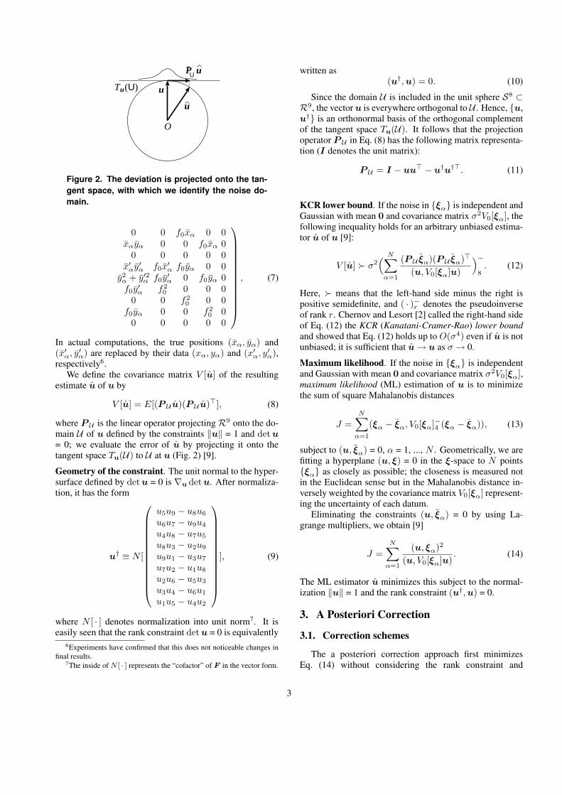
Figure 2. The deviation is projected onto the tan-gent space, with which we identify the noise do-main.

0 0 f0xα 0 0xαyα 0 0 f0xα 0

0 0 0 0 0x′

αy′α f0x

′α f0yα 0 0

y2α + y′2

α f0y′α 0 f0yα 0

f0y′α f2

0 0 0 00 0 f2

0 0 0f0yα 0 0 f2

0 00 0 0 0 0

, (7)

In actual computations, the true positions (xα, yα) and(x′

α, y′α) are replaced by their data (xα, yα) and (x′

α, y′α),

respectively6.We define the covariance matrix V [u] of the resulting

estimate u of u by

V [u] = E[(P U u)(P U u)>], (8)

where P U is the linear operator projecting R9 onto the do-main U of u defined by the constraints ‖u‖ = 1 and det u= 0; we evaluate the error of u by projecting it onto thetangent space Tu(U) to U at u (Fig. 2) [9].

Geometry of the constraint. The unit normal to the hyper-surface defined by det u = 0 is ∇u detu. After normaliza-tion, it has the form

u† ≡ N [

u5u9 − u8u6

u6u7 − u9u4

u4u8 − u7u5

u8u3 − u2u9

u9u1 − u3u7

u7u2 − u1u8

u2u6 − u5u3

u3u4 − u6u1

u1u5 − u4u2

], (9)

where N [ · ] denotes normalization into unit norm7. It iseasily seen that the rank constraint det u = 0 is equivalently

6Experiments have confirmed that this does not noticeable changes infinal results.

7The inside of N [ · ] represents the “cofactor” of F in the vector form.

written as(u†, u) = 0. (10)

Since the domain U is included in the unit sphere S8 ⊂R9, the vector u is everywhere orthogonal to U . Hence, {u,u†} is an orthonormal basis of the orthogonal complementof the tangent space Tu(U). It follows that the projectionoperator P U in Eq. (8) has the following matrix representa-tion (I denotes the unit matrix):

P U = I − uu> − u†u†>. (11)

KCR lower bound. If the noise in {ξα} is independent andGaussian with mean 0 and covariance matrix σ2V0[ξα], thefollowing inequality holds for an arbitrary unbiased estima-tor u of u [9]:

V [u] Â σ2( N∑

α=1

(P U ξα)(P U ξα)>

(u, V0[ξα]u)

)−

8. (12)

Here, Â means that the left-hand side minus the right ispositive semidefinite, and ( · )−r denotes the pseudoinverseof rank r. Chernov and Lesort [2] called the right-hand sideof Eq. (12) the KCR (Kanatani-Cramer-Rao) lower boundand showed that Eq. (12) holds up to O(σ4) even if u is notunbiased; it is sufficient that u → u as σ → 0.

Maximum likelihood. If the noise in {ξα} is independentand Gaussian with mean 0 and covariance matrix σ2V0[ξα],maximum likelihood (ML) estimation of u is to minimizethe sum of square Mahalanobis distances

J =N∑

α=1

(ξα − ξα, V0[ξα]−4 (ξα − ξα)), (13)

subject to (u, ξα) = 0, α = 1, ..., N . Geometrically, we arefitting a hyperplane (u, ξ) = 0 in the ξ-space to N points{ξα} as closely as possible; the closeness is measured notin the Euclidean sense but in the Mahalanobis distance in-versely weighted by the covariance matrix V0[ξα] represent-ing the uncertainty of each datum.

Eliminating the constraints (u, ξα) = 0 by using La-grange multipliers, we obtain [9]

J =N∑

α=1

(u, ξα)2

(u, V0[ξα]u). (14)

The ML estimator u minimizes this subject to the normal-ization ‖u‖ = 1 and the rank constraint (u†,u) = 0.

3. A Posteriori Correction

3.1. Correction schemes

The a posteriori correction approach first minimizesEq. (14) without considering the rank constraint and

3

then modifies the resulting solution u so as to satisfy it(Fig. 1(a)).

SVD correction. A naive idea is to compute the singularvalue decomposition (SVD) of the computed fundamentalmatrix and replace the smallest singular value by 0, result-ing in a matrix of rank 2 “closest” to the original one inFrobenius norm [6]. We call this SVD correction.

Optimal correction. A more sophisticated method is theoptimal correction [9, 16]. According to the statistical opti-mization theory [9], the covariance matrix V [u] of the rankunconstrained solution u can be evaluated, so u is movedin the direction of the mostly likely fluctuation implied byV [u] until it satisfies the rank constraint (Fig. 1(a)). Theprocedure goes as follows [9]:

1. Compute the following 9 × 9 matrix M :

M =N∑

α=1

ξαξ>α

(u, V0[ξα]u). (15)

2. Compute the matrix V0[u] as follows:

V0[u] = (P uMP u)−8 , (16)

whereP u = I − uu>. (17)

3. Update the solution u as follows (u† is defined byEq. (9) for u):

u ← N [u − 13

(u, u†)V0[u]u†

(u†, V0[u]u†)]. (18)

4. If (u, u†) ≈ 0, return u and stop. Else, update P u andV0[u] in the form

P u ← I − uu>, V0[u] ← P uV0[u]P u, (19)

and go back to Step 3.

Explanation. Since u is a unit vector, its endpoint is onthe unit sphere S8 in R9. Eq. (18) is essentially the New-ton iteration formula for displacing u in the direction in thetangent space Tu(S8) along which J is least increased sothat (u†, u) = 0 is satisfied. However, u deviates from S8

by a small distance of high order as it proceeds in Tu(S8),so we pull it back onto S8 using the operator N [ · ]. Fromthat point, the same procedure is repeated until (u†, u) = 0.However, the normalized covariance matrix V0[u] is definedin the tangent space Tu(S8), which changes as u moves.Eq. (19) corrects it so that V0[u] has the domain Tu(S8) atthe displaced point u.

3.2. Unconstrained ML

Before imposing the rank constraint, we need to solveunconstrained minimization of Eq. (14), for which manymethod exist including FNS [3], HEIV [14], and the pro-jective Gauss-Newton iterations [11]. Their convergenceproperties were studies in [11].

FNS. The FNS (Fundamental Numerical Scheme) of Cho-jnacki et al. [3] is based on the fact that the derivative ofEq. (14) with respect to u has the form

∇uJ = 2Xu, (20)

where X has the following form [3]:

X = M − L, (21)

M =N∑

α=1

ξαξ>α

(u, V0[ξα]u), L =

N∑α=1

(u, ξα)2V0[ξα](u, V0[ξα]u)2

.

(22)The FNS solves

Xu = 0. (23)

by the following iterations [3, 11]:

1. Initialize u.2. Compute the matrix X in Eq. (21).3. Solve the eigenvalue problem

Xu′ = λu′, (24)

and compute the unit eigenvector u′ for the smallesteigenvalue λ.

4. If u′ ≈ u up to sign, return u′ and stop. Else, let u ←u′ and go back to Step 2.

Originally, the eigenvalue closest to 0 was chosen [3] inStep 3. Later, Chojnacki, et al. [5] pointed out that thechoice of the smallest eigenvalue improves the convergence.This was also confirmed by the experiments of Kanatani andSugaya [11].

Whichever eigenvalue is chosen for λ, we have λ = 0after convergence. In fact, convergence means

Xu = λu (25)

for some u. Computing the inner product with u on bothsides, we have

(u, Xu) = λ, (26)

but from Eq. (30) we have the identity (u, Xu) = 0 in u.Hence, λ = 0, and u is the desired solution.

HEIV. Equation (23) is rewritten as

Mu = Lu. (27)

4

We introduce a new 8-D vector v, 8-D data vectors zα, andtheir 8 × 8 normalized covariance matrices V|0[zα] by

ξα =(

zα

f20

), u =

(v

F33

),

V0[ξα] =(

V0[zα] 00> 0

), (28)

and define 8 × 8 matrices

M =N∑

α=1

zαz>α

(v, V0[zα]v), L =

N∑α=1

(v, zα)2V0[zα](v, V0[zα]v)2

,

(29)where we put

zα = zα − z,

z =N∑

α=1

zα

(v, V0[zα]v)

/N∑

β=1

1(v, V0[zβ ]v)

. (30)

Then, Eq. (27) splits into the following two equations [5,14]:

Mv = Lv, (v, z) + f20 F33 = 0. (31)

Hence, if an 8-D vector v that satisfies the first equation iscomputed, the second equation gives F33, and we obtain

u = N[( v

F33

)]. (32)

The HEIV (Heteroscedastic Errors-in-Variable) of Leedanand Meer [14] computes the vector v that satisfies the firstof Eqs. (31) by the following iterations [5, 14]:

1. Initialize v.2. Compute the matrices M and L in Eqs. (29).3. Solve the generalized eigenvalue problem

Mv′ = λLv′, (33)

and compute the unit generalized eigenvector v′ for thesmallest generalized eigenvalue λ.

4. If v′ ≈ v except for sign, return v′ and stop. Else, letv ← v′ and go back to Step 2.

In order to reach the solution of Eqs. (31), it appears naturalto choose the generalized eigenvalue λ in Eq. (33) to be theone closest 1. However, Leedan and Meer [14] observedthat choosing the smallest one improves the convergenceperformance. This was also confirmed by the experimentsof Kanatani and Sugaya [11].

Whichever generalized eigenvalue is chosen for λ, wehave λ = 1 after convergence. In fact, convergence means

Mv = λLv (34)

for some v. Computing the inner product of both sides withv, we have

(v,Mv) = λ(v, Lv), (35)

but from Eqs. (29) we have the identity (v,Mv) = (v, Lv)in v. Hence, λ = 1, and u is the desired solution.

Projective Gauss-Newton iterations. Since the gradient∇uJ is given by Eq. (20), we can minimize the function Jby Newton iterations. If we evaluate the Hessian ∇2

uJ , theincrement ∆u in u is determined by solving

(∇2uJ)∆u = −∇uJ. (36)

However, ∇2uJ is singular, since J is constant in the direc-

tion of u (see Eq. (14)). Hence, the solution is indetermi-nate. However, if we use pseudoinverse and compute

∆u = −(∇2uJ)−8 ∇uJ, (37)

we obtain a solution orthogonal to u.Differentiating Eq. (20) and introducing Gauss-Newton

approximation (i.e., ignoring terms that contain (u, ξα)),we see that the Hessian is nothing but the matrix 2M inEqs. (22). We enforce M to have eigenvalue 0 for u, usingthe projection matrix

P u = I − uu> (38)

onto the direction orthogonal to u. The iteration proceduregoes as follows:

1. Initialize u.2. Compute

u′ = N [u − (P uMP u)−8 (M − L)u]. (39)

3. If u′ ≈ u, return u′ and stop. Else, let u ← u′ and goback to Step 2.

3.3. Initialization

The FNS, the HEIV, and the projective Gauss-Newtonare all iterative method, so they require initial values. Thebest known non-iterative procedures are the least squaresand the Taubin method.

Least squares (LS). This is the most popular method, alsoknown as the algebraic distance minimization or the 8-pointalgorithm [6]. Approximating the denominators in Eq. (14)by a constant, we minimize

JLS =N∑

α=1

(u, ξα)2 = (u,MLSu), (40)

where we define

MLS =N∑

α=1

ξαξ>α . (41)

5

Equation (40) is minimized by the unit eigenvalue u ofMLS for the smallest eigenvalue.

Taubin’s method. Replacing the denominators in Eq. (14)by their average, we minimize the following function8 [23]:

JTB =∑N

α=1(u, ξα)2∑Nα=1(u, V0[ξα]u)

=(u, MLSu)(u, NTBu)

. (42)

The matrix NTB has the form

NTB =N∑

α=1

V0[ξα]. (43)

Equation (42) is minimized by solving the generalizedeigenvalue problem

MLSu = λNTBu (44)

for the smallest generalized eigenvalue. However, we can-not directly solve this, because NTB is not positive defi-nite. So, we decompose ξα, u, and V0[ξα] in the form ofEqs. (28) and define 8 × 8 matrices MLS and NTB by

MLS =N∑

α=1

zαz>α , NLS =

N∑α=1

V0[zα], (45)

where

zα = zα − z, z =1N

N∑α=1

zα. (46)

Then, Eq. (44) splits into two equations

MLSv = λNTBv, (v, z) + f20 F33 = 0. (47)

We compute the unit generalized eigenvector v of the firstequation for the smallest generalized eigenvalue λ. Thesecond equation gives F33, and u is given in the form ofEq. (32). It has been shown that Taubin’s method producesa very accurate close to the unconstrained ML solution [11].

4. Internal Access

The fundamental matrix F has nine elements, on whichthe normalization ‖F ‖ = 1 and the rank constraint det u =0 are imposed. Hence, it has seven degrees of freedom. Theinternal access minimizes Eq. (14) by searching the reduced7-D parameter space (Fig. 1(b)).

Many types of 7-degree parameterizations have beenobtained, e.g., by algebraic elimination of the rank con-straint or by expressing the fundamental matrix in termsof epipoles [20, 25], but the resulting expressions are com-plicated, and the geometric meaning of the individual un-knowns are not clear. This was overcome by Bartoli and

8Taubin [23] did not take the covariance matrix into account. This is amodification of his method.

Sturm [1], who regarded the SVD of F as its parameter-ization. Their expression is compact, and each parameterhas its geometric meaning. However, they included, in ad-dition to F , the tentatively reconstructed 3-D positions ofthe observed feature points, the relative positions of thetwo cameras, and their intrinsic parameters as unknownsand minimized the reprojection error; such an approach isknown as bundle adjustment. Since the tentative 3-D recon-struction from two images is indeterminate, they chose theone for which the first camera matrix is in a particular form(“canonical form”).

Here, we point out that we can avoid this complication bydirectly minimizing Eq. (14) by the Levenberg-Marquardt(LM) method, using the parameterization of Bartoli andSturm [1] (a preliminary version was presented in our con-ference paper [22]).

The fundamental matrix F has rank 2, so its SVD hasthe form

F = Udiag(σ1, σ2, 0)V>, (48)

where U and V are orthogonal matrices, and σ1 and σ2

are the singular values. Since the normalization ‖F ‖2 = 1is equivalent to σ2

1 + σ22 = 1 (Appendix A), we adopt the

following parameterization9:

σ1 = cos θ, σ2 = sin θ. (49)

The orthogonal matrices U and V have three degrees offreedom each, so they and θ constitute the seven degreesof freedom. However, the analysis becomes complicated ifU and V are directly expressed in three parameters each(e.g., the Euler angles or the rotations around each coordi-nate axis). Following Bartoli and Sturm [1], we adopt the“Lie algebraic method”: we represent the “increment” in Uand V by three parameters each. Let ω1, ω2, and ω3 rep-resent the increment in U , and ω′

1, ω′2, and ω′

3 in V . Thederivatives of Eq. (14) with respect to them are as follows(Appendix A):

∇ωJ = 2F>UXu, ∇ω′J = 2F>

V Xu. (50)

Here, X is the matrix in Eq. (21), and F U , and F V aredefined by

F U =

0 F31 −F21

0 F32 −F22

0 F33 −F23

−F31 0 F11

−F32 0 F12

−F33 0 F13

F21 −F11 0F22 −F12 0F23 −F13 0

,

9Bartoli and Sturm [1] took the ratio γ = σ2/σ1 as a variable. Here,we adopt the angle θ for the symmetry. As is well known, it has the valueπ/4 (i.e., σ1 = σ2) if the principal point is at the origin (0, 0) and if thereare no image distortions [7, 9].

6

F V =

0 F13 −F12

−F13 0 F11

F12 −F11 00 F23 −F22

−F23 0 F21

F22 −F21 00 F33 −F32

−F33 0 F31

F32 −F31 0

. (51)

The derivative of Eq. (14) with respect to θ has the form(Appendix A)

∂J

∂θ= 2(uθ,Xu), (52)

where we define

uθ =

U12V12 cos θ − U11V11 sin θU12V22 cos θ − U11V21 sin θU12V32 cos θ − U11V31 sin θU22V12 cos θ − U21V11 sin θU22V22 cos θ − U21V21 sin θU22V32 cos θ − U21V31 sin θU32V12 cos θ − U31V11 sin θU32V22 cos θ − U31V21 sin θU32V32 cos θ − U31V31 sin θ

. (53)

Adopting Gauss-Newton approximation, which amounts toignoring terms involving (u, ξα), we obtain the secondderivatives as follows (Appendix A):

∇2ωJ = 2F>

UMF U , ∇2ω′J = 2F>

V MF V ,

∇ωω′J = 2F>UMF V , 2

∂J2

∂θ2= (uθ, Muθ),

∂∇ωJ

∂θ= 2F>

UMuθ,∂∇ω′J

∂θ= 2F>

V Muθ. (54)

The 7-parameter LM search goes as follows:

1. Initialize F = Udiag(cos θ, sin θ, 0)V>.2. Compute J in Eq. (14), and let c = 0.0001.3. Compute F U , F V , and uθ in Eqs. (51) and (53).4. Compute X in Eq. (21), the first derivatives in

Eqs. (50) an (52), and the second derivatives inEqs. (54).

5. Compute the following matrix H:

H =

∇2ωJ ∇ωω′J ∂∇ωJ/∂θ

(∇ωω′J)> ∇2ω′J ∂∇ω′J/∂θ

(∂∇ωJ/∂θ)> (∂∇ω′J/∂θ)> ∂J2/∂θ2

.

(55)6. Solve the 7-D simultaneous linear equations

(H + cD[H])

ωω′

∆θ

= −

∇ωJ∇ω′J∂J/∂θ

, (56)

for ω, ω′, and ∆θ, where D[ · ] denotes the diagonalmatrix obtained by taking out only the diagonal ele-ments.

7. Update U , V , and θ by

U ′ = R(ω)U , V ′ = R(ω′)V , θ′ = θ + ∆θ, (57)

where R(ω) denotes rotation around N [ω] by angle‖ω‖.

8. Update F as follows:

F ′ = U ′diag(cos θ′, sin θ′, 0)V ′>. (58)

9. Let J ′ be the value of Eq. (14) for F ′.10. Unless J ′ < J or J ′ ≈ J , let c ← 10c, and go back to

Step 6.11. If F ′ ≈ F , return F ′ and stop. Else, let F ← F ′, U

← U ′, V ← V ′, θ ← θ′, and c ← c/10, and go back toStep 3.

5. External Access

The external access approach does iterations in the 9-Du-space in such a way that an optimal solution satisfying therank constraint automatically results (Fig. 1(c)). The con-cept dates back to such heuristics as introducing penaltiesto the violation of the constraints or projecting the solutiononto the surface of the constraints in the course of iterations,but it is Chojnacki et al. [4] that first presented a systematicscheme, which they called CFNS.

Stationarity Condition. According to the variational prin-ciple, the necessary and sufficient condition for the functionJ to be stationary at a point u in S8 in R9 is that its gradient∇uJ is orthogonal to the hypersurface defined by det u =0 or by Eq. (10), and its surface normal is given by u† inEq. (9). However, ∇uJ = Xu is always tangent to S8, be-cause of the identity (u,∇uJ) = (u, Xu) = 0 in u. Hence,∇uJ should be parallel to u†. This means that if we definethe projection matrix

P u† = I − u†u†> (59)

onto the direction orthogonal to u†, the stationarity condi-tion is written as

P u†Xu = 0. (60)

The rank constraint of Eq. (10) is written as P u†u = u.Combined with Eq. (60), the desired solution should besuch that

Yu = 0, P u†u = u, (61)

where we define

Y = P u†XP u† . (62)

CFNS. Chojnacki et al. [4] showed that the stationarity con-dition of Eqs. (61) is written as a single equation in the form

Qu = 0, (63)

where Q is a rather complicated symmetric matrix. Theyproposed to solve this by iterations in the same form as theirFNS and called it CFNS (Constrained FNS):

7

1. Initialize u.2. Compute the matrix Q.3. Solve the eigenvalue problem

Qu′ = λu′, (64)

and compute the unit eigenvector u′ for the eigenvalueλ closest to 0.

4. If u′ ≈ u up to sign, return u′ and stop. Else, let u ←u′, and go back to Step 2.

Infinitely many candidates exist for the matrix Q withwhich the problem is written as Eq. (13), but not all of themallow the above iterations to converge. Chojnacki et al. [4]gave one (see Appendix B), but the derivation is not writtenin their paper. Later, we show that CFNS does not necessar-ily converge to a correct solution.

EFNS. We now present a new iterative scheme, which wecall EFNS (Extended FNS), for solving Eqs. (61) (a prelim-inary version was presented in a more abstract form in ourconference paper [12]). The procedure goes as follows:

1. Initialize u.2. Compute the matrix X in Eq. (21).3. Computer the projection matrix P u† (u† is defined by

Eq. (9)):P u† = I − u†u†>. (65)

4. Compute the matrix Y in Eq. (62).5. Solve the eigenvalue problem

Yv = λv, (66)

and compute the two unit eigenvectors v1 and v2 forthe smallest eigenvalues in absolute terms.

6. Compute the following vector u:

u = (u, v1)v1 + (u, v2)v2 (67)

7. Computeu′ = N [P u†u]. (68)

8. If u′ ≈ u, return u′ and stop. Else, let u ← N [u+u′]and go back to Step 2.

Justification. We first show that when the above itera-tions have converged, the eigenvectors v1 and v2 both haveeigenvalue 0. From the definition of Y in Eq. (62) and P u†

in Eq. (65), u† is always an eigenvector of Y with eigen-value 0 and is equal to u† up to sign. This means that ei-ther v1 or v2 has eigenvalue 0. Suppose one, say v1, hasnonzero eigenvalue λ ( 6= 0). Then, v2 = ±u†.

By construction, the vector u in Eq. (67) belongs to thelinear span of v1 and v2 (= ±u†) and the vector u′ inEq. (68) is a projection of u within that linear span onto thedirection orthogonal to u†. Hence, it coincides with ±v1.

Figure 3. Simulated images of planar grid sur-faces.

The iterations converge when u = u′ (= ±v1). Thus, v1 isan eigenvector of Y with eigenvalue λ. Hence, u also satis-fies Eq. (66). Computing the inner product with u on bothsides, we have

(u,Yu) = λ. (69)

On the other hand, u (= ±v1) is orthogonal to u† (= ±v2),so

P u†u = u. (70)

Hence,

(u, Yu) = (u,P u†XP u†u) = (u, Xu) = 0, (71)

since (u, Xu) = 0 is an identity in u (see Eqs. (30)).Eqs. (69) and (71) contradict our assumption that λ 6= 0.So, v1 is also an eigenvector of Y with eigenvalue 0. 2

It follows that both Xu = 0 and Eq. (70) hold, and thusu is the desired solution. Of course, this conclusion relieson the premise that the iterations converge. According toour experience, if we let u ← u′ in Step 9, the next valueof u′ computed in Step 8 often reverts to the former valueof u, falling in infinite looping. So, we update u to the“midpoint” (u′ + u)/2 and normalized it to a unit vectorN [u′ + u] in Step 9. By this, the iterations converged in allof our experiments.

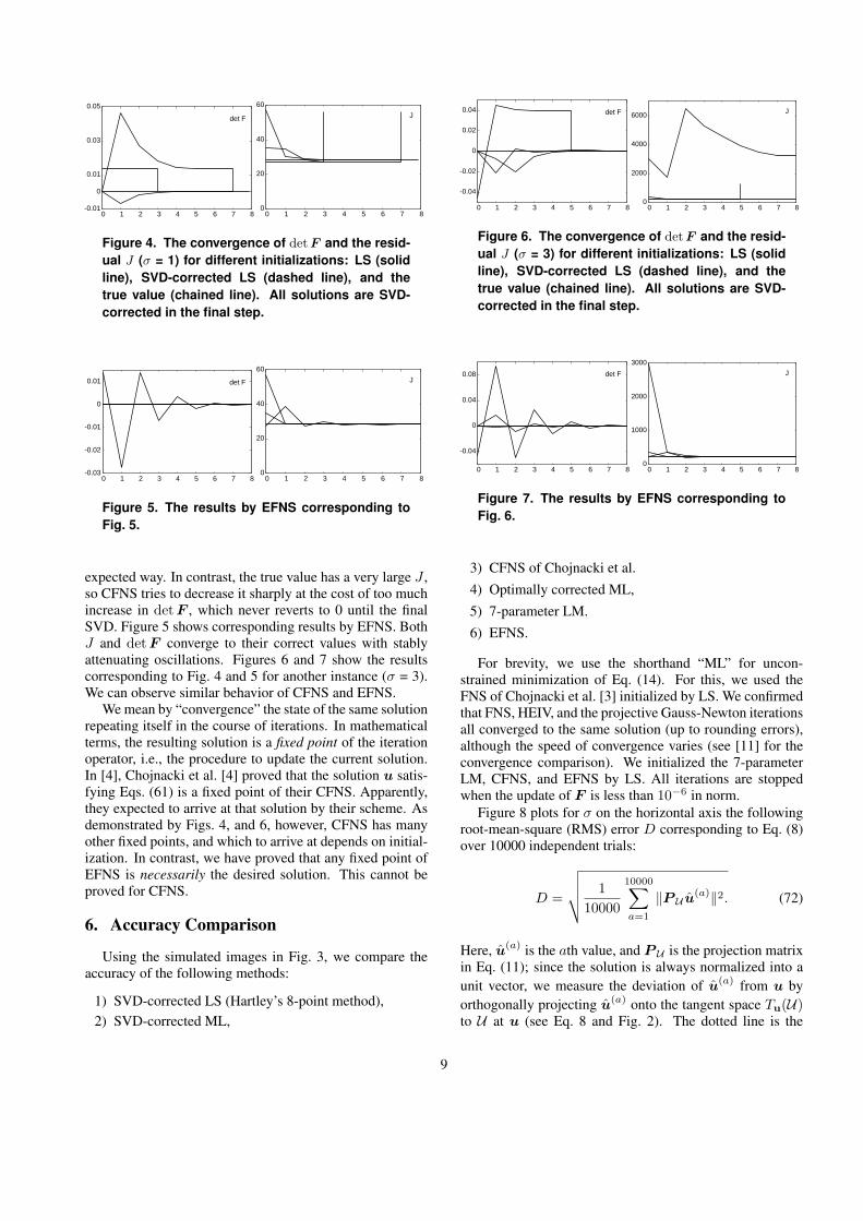
CFNS vs. EFNS. Figure 3 shows simulated images of twoplanar grid surfaces viewed from different angles. The im-age size is 600×600 pixels with 1200 pixel focal length. Weadded random Gaussian noise of mean 0 and standard devi-ation σ to the x- and y-coordinates of each grid point inde-pendently and from them computed the fundamental matrixby CFNS and EFNS.

Figure 4 shows a typical instance (σ = 1) of the con-vergence of the determinant det F and the residual J fromdifferent initial values. In the final step, detF is forced tobe 0 by SVD, as prescribed by Chojnacki et al. [4]. Thedotted lines show the values to be converged.

The LS solution has a very low residual J , since the rankconstraint det F = 0 is ignored. So, J needs to be increasedto achieve detF = 0, but CFNS fails to do so. As a result,det F remains nonzero and drops to 0 by the final SVD cor-rection, causing a sudden jump in J . If we start from SVD-corrected LS, the residual J first increases, making det Fnonzero, but in the end both J and det F converge in an

8

-0.01

0

0.01

0.03

0.05

0 1 2 3 4 5 6 7 8

det F

0

20

40

60

0 1 2 3 4 5 6 7 8

J

Figure 4. The convergence of det F and the resid-ual J (σ = 1) for different initializations: LS (solidline), SVD-corrected LS (dashed line), and thetrue value (chained line). All solutions are SVD-corrected in the final step.

-0.03

-0.02

-0.01

0

0.01

0 1 2 3 4 5 6 7 8

det F

0

20

40

60

0 1 2 3 4 5 6 7 8

J

Figure 5. The results by EFNS corresponding toFig. 5.

expected way. In contrast, the true value has a very large J ,so CFNS tries to decrease it sharply at the cost of too muchincrease in det F , which never reverts to 0 until the finalSVD. Figure 5 shows corresponding results by EFNS. BothJ and det F converge to their correct values with stablyattenuating oscillations. Figures 6 and 7 show the resultscorresponding to Fig. 4 and 5 for another instance (σ = 3).We can observe similar behavior of CFNS and EFNS.

We mean by “convergence” the state of the same solutionrepeating itself in the course of iterations. In mathematicalterms, the resulting solution is a fixed point of the iterationoperator, i.e., the procedure to update the current solution.In [4], Chojnacki et al. [4] proved that the solution u satis-fying Eqs. (61) is a fixed point of their CFNS. Apparently,they expected to arrive at that solution by their scheme. Asdemonstrated by Figs. 4, and 6, however, CFNS has manyother fixed points, and which to arrive at depends on initial-ization. In contrast, we have proved that any fixed point ofEFNS is necessarily the desired solution. This cannot beproved for CFNS.

6. Accuracy Comparison

Using the simulated images in Fig. 3, we compare theaccuracy of the following methods:

1) SVD-corrected LS (Hartley’s 8-point method),2) SVD-corrected ML,

-0.04

-0.02

0

0.02

0.04

0 1 2 3 4 5 6 7 8

det F

0

2000

4000

6000

0 1 2 3 4 5 6 7 8

J

Figure 6. The convergence of det F and the resid-ual J (σ = 3) for different initializations: LS (solidline), SVD-corrected LS (dashed line), and thetrue value (chained line). All solutions are SVD-corrected in the final step.

-0.04

0

0.04

0.08

0 1 2 3 4 5 6 7 8

det F

0

1000

2000

3000

0 1 2 3 4 5 6 7 8

J

Figure 7. The results by EFNS corresponding toFig. 6.

3) CFNS of Chojnacki et al.4) Optimally corrected ML,5) 7-parameter LM.6) EFNS.

For brevity, we use the shorthand “ML” for uncon-strained minimization of Eq. (14). For this, we used theFNS of Chojnacki et al. [3] initialized by LS. We confirmedthat FNS, HEIV, and the projective Gauss-Newton iterationsall converged to the same solution (up to rounding errors),although the speed of convergence varies (see [11] for theconvergence comparison). We initialized the 7-parameterLM, CFNS, and EFNS by LS. All iterations are stoppedwhen the update of F is less than 10−6 in norm.

Figure 8 plots for σ on the horizontal axis the followingroot-mean-square (RMS) error D corresponding to Eq. (8)over 10000 independent trials:

D =

√√√√ 110000

10000∑a=1

‖P U u(a)‖2. (72)

Here, u(a) is the ath value, and P U is the projection matrixin Eq. (11); since the solution is always normalized into aunit vector, we measure the deviation of u(a) from u byorthogonally projecting u(a) onto the tangent space Tu(U)to U at u (see Eq. 8 and Fig. 2). The dotted line is the

9

0

0.1

0.2

0 1 2 3 4σ

1

23

4 6

5

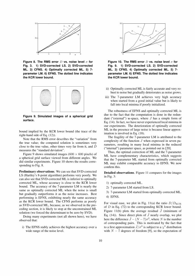
Figure 8. The RMS error D vs. noise level σ forFig. 3. 1) SVD-corrected LS. 2) SVD-correctedML. 3) CFNS. 4) Optimally corrected ML. 5) 7-parameter LM. 6) EFNS. The dotted line indicatesthe KCR lower bound.

Figure 9. Simulated images of a spherical gridsurface.

bound implied by the KCR lower bound (the trace of theright-hand side of Eq. (12)).

Note that the RMS error describes the “variation” fromthe true value; the computed solution is sometimes veryclose to the true value, other times very far from it, and Dmeasures the “standard deviation”.

Figure 9 shows simulated images (600 × 600 pixels) ofa spherical grid surface viewed from different angles. Wedid similar experiments. Figure 10 shows the results corre-sponding to Fig. 8.

Preliminary observations. We can see that SVD-correctedLS (Hartley’s 8-point algorithm) performs very poorly. Wecan also see that SVD-corrected ML is inferior to optimallycorrected ML, whose accuracy is close to the KCR lowerbound. The accuracy of the 7-parameter LM is nearly thesame as optimally corrected ML when the noise is smallbut gradually outperforms it as the noise increases. Bestperforming is EFNS, exhibiting nearly the same accuracyas the KCR lower bound. The CFNS performs as poorlyas SVD-corrected ML, because, as we observed in the pre-ceding section, it is likely to stop at the unconstrained MLsolution (we forced the determinant to be zero by SVD).

Doing many experiments (not all shown here), we haveobserved that:

i) The EFNS stably achieves the highest accuracy over awide range of the noise level.

0

0.1

0.2

0 1 2σ

1

2

3

4

5

6

Figure 10. The RMS error D vs. noise level σ forFig. 9. 1) SVD-corrected LS. 2) SVD-correctedML. 3) CFNS. 4) Optimally corrected ML. 5) 7-parameter LM. 6) EFNS. The dotted line indicatesthe KCR lower bound.

ii) Optimally corrected ML is fairly accurate and very ro-bust to noise but gradually deteriorates as noise grows.

iii) The 7-parameter LM achieves very high accuracywhen started from a good initial value but is likely tofall into local minima if poorly initialized.

The robustness of EFNS and optimally corrected ML isdue to the fact that the computation is done in the redun-dant (“external”) u-space, where J has a simple form ofEq. (14). In fact, we have never experienced local minima inour experiments. The deterioration of optimally correctedML in the presence of large noise is because linear approx-imation is involved in Eq. (18).

The fragility of the 7-parameter LM is attributed to thecomplexity of the function J when expressed in seven pa-rameters, resulting in many local minima in the reduced(“internal”) parameter space, as pointed out in [20].

Thus, the optimal correction of ML and the 7-parameterML have complementary characteristics, which suggeststhat the 7-parameter ML started from optimally correctedML may exhibit comparable accuracy to EFNS. We nowconfirm this.

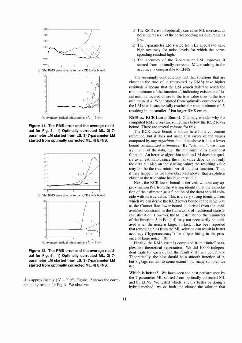
Detailed observations. Figure 11 compares for the imagesin Fig. 3:

1) optimally corrected ML.2) 7-parameter LM started from LS.3) 7-parameter LM started from optimally corrected ML.4) EFNS.

For visual ease, we plot in Fig. 11(a) the ratio D/DKCR

of D in Eq. (72) to the corresponding KCR lower bound.Figure 11(b) plots the average residual J (minimum ofEq. (14)). Since direct plots of J nearly overlap, we plothere the difference J − (N − 7)σ2, where N is the numberof corresponding pairs. This is motivated by the fact thatto a first approximation J/σ2 is subject to a χ2 distributionwith N − 7 degrees of freedom [9], so the expectation of

10

0.96

0.98

1

1.02

1.04

1.06

1.08

0 1 2 3 4σ

1

23

4

(a) The RMS error relative to the KCR lower bound.

-2

0

2

4

6

8

10

12

0 1 2 3 4σ

2

1 3

4

(b) Average residual minus minus (N − 7)σ2.

Figure 11. The RMS error and the average resid-ual for Fig. 3. 1) Optimally corrected ML. 2) 7-parameter LM started from LS. 3) 7-parameter LMstarted from optimally corrected ML. 4) EFNS.

0.9

1

1.1

1.2

1.3

1.4

1.5

1.6

1.7

1.8

0 1 2

1

2

3 4

σ

(a) The RMS error relative to the KCR lower bound.

-5

0

5

10

15

20

0 1 2

12

3 4

σ

(b) Average residual minus minus (N − 7)σ2.

Figure 12. The RMS error and the average resid-ual for Fig. 9. 1) Optimally corrected ML. 2) 7-parameter LM started from LS. 3) 7-parameter LMstarted from optimally corrected ML. 4) EFNS.

J is approximately (N − 7)σ2. Figure 12 shows the corre-sponding results for Fig. 9. We observe:

i) The RMS error of optimally corrected ML increases asnoise increases, yet the corresponding residual remainslow.

ii) The 7-parameter LM started from LS appears to havehigh accuracy for noise levels for which the corre-sponding residual high.

iii) The accuracy of the 7-parameter LM improves ifstarted from optimally corrected ML, resulting in theaccuracy is comparable to EFNS.

The seemingly contradictory fact that solutions that arecloser to the true value (measured by RMS) have higherresiduals J means that the LM search failed to reach thetrue minimum of the function J , indicating existence of lo-cal minima located closer to the true value than to the trueminimum of J . When started from optimally corrected ML,the LM search successfully reaches the true minimum of J ,resulting in the smaller J but larger RMS errors.

RMS vs. KCR Lower Bound. One may wonder why thecomputed RMS errors are sometimes below the KCR lowerbound. There are several reasons for this.

The KCR lower bound is shown here for a convenientreference, but it does not mean that errors of the valuescomputed by any algorithm should be above it; it is a lowerbound on unbiased estimators. By “estimator”, we meana function of the data, e.g., the minimizer of a given costfunction. An iterative algorithm such as LM does not qual-ify as an estimator, since the final value depends not onlythe data but also on the starting value; the resulting valuemay not be the true minimizer of the cost function. Thus,it may happen, as we have observed above, that a solutioncloser to the true value has higher residual.

Next, the KCR lower bound is derived, without any ap-proximation [9], from the starting identity that the expecta-tion of the estimator (as a function of the data) should coin-cide with its true value. This is a very strong identity, fromwhich we can derive the KCR lower bound in the same wayas the Cramer-Rao lower bound is derived from the unbi-asedness constraint in the framework of traditional statisti-cal estimation. However, the ML estimator or the minimizerof the function J in Eq. (14) may not necessarily be unbi-ased when the noise is large. In fact, it has been reportedthat removing bias from the ML solution can result in betteraccuracy (“hyperaccuracy”) for ellipse fitting in the pres-ence of large noise [10].

Finally, the RMS error is computed from “finite” sam-ples, not theoretical expectation. We did 10000 indepen-dent trials for each σ, but the result still has fluctuations.Theoretically, the plot should be a smooth function of σ,but zigzags remain to some extent how many samples weuse.

Which is better?. We have seen the best performance bythe 7-parameter ML started from optimally corrected MLand by EFNS. We tested which is really better by doing ahybrid method: we do both and choose the solution that

11

0

1

0 1 2 3 4

0.5

σ

Figure 13. The ratio of the solution being chosenfor Fig. 3. Solid line: 7-parameter LM started fromoptimally corrected ML. Dashed line: EFNS.

0

1

0 0.5 1 1.5 2

0.5

σ

Figure 14. The ratio of the solution being chosenfor Fig. 9. Solid line: 7-parameter LM started fromoptimally corrected ML. Dashed line: EFNS.

has a smaller value of J . Figure 13 plots the ratio of eachsolution being chosen for the images in Fig. 3; Figure 14plots the corresponding result for Fig. 9. As we can see,the two are completely even; there is no distinction betweenthem.

7. Bundle Adjustment (Gold Standard)

There is a subtle point to be clarified in the discussion ofSect. 2. The transition from Eq. (13) to Eq. (14) is exact;no approximation is involved. Although terms of O(σ4)are omitted and the true values are replaced by their data inEq. (7), it is numerically confirmed that these do not affectthe final results in any noticeable way.

However, although the “analysis” may be exact, the “in-terpretation” is not strict. Namely, despite the fact thatEq. (14) is the (squared) Mahalanobis distance in the ξ-space, its minimization can be ML only when the noise inthe ξ-space is Gaussian, because then and only then is thelikelihood proportional to e−J/constant. Strictly speaking,if the noise in the image plane is Gaussian, the transformednoise in the ξ-space is no longer Gaussian, so the provisothat “If the noise in {ξα} is ...” above Eq. (13) (and forthe KCR lower bound of Eq. (12), too) does not necessar-ily hold, and minimizing Eq. (14) is not strictly ML in theimage plane.

In order to test how much difference is incurred bythis, we minimize the Mahalanobis distance in the {x, x′}-space, called the reprojection error. This approach was en-dorsed by Hartley and Zisserman [7], who called it the GoldStandard.

This is usually done as search in a high-dimensional pa-rameter space, as done by Bartoli and Sturm [1], computingtentative 3-D reconstruction and adjusting the reconstructedshape, the camera positions, and the intrinsic parameters sothat the resulting projection images are as close to the inputimages as possible. Such a strategy is called bundle adjust-ment.

Here, we present a new numerical scheme for directlyminimizing the reprojection error without reference to anytentative 3-D reconstruction (this result has not been pre-sented anywhere else). Then, we compare its accuracy withthose methods we described so far.

Problem. We minimize the reprojection error

E =N∑

α=1

(‖xα − xα‖2 + ‖x′

α − x′α‖2

), (73)

with respect to xα, xα, α = 1, ..., N , and F (constrained tobe ‖F ‖ = 1 and detF = 0) subject to the epipolar constraint

(xα, F x′α) = 0, α = 1, ..., N. (74)

First approximation. Instead of estimating xα and x′α di-

rectly, we express them as

xα = xα − ∆xα, x′α = x′

α − ∆x′α, (75)

and estimate the correction terms ∆xα and ∆x′α. Substi-

tuting Eqs. (75) into Eq. (73), we have

E =N∑

α=1

(‖∆xα‖2 + ‖∆x′

α‖2). (76)

The epipolar equation of Eq. (74) becomes

(xα − ∆xα, F (x′α − ∆x′

α)) = 0. (77)

Ignoring the second order terms in the correction terms, weobtain to a first approximation

(Fx′α, ∆xα) + (F>xα, ∆x′

α) = (xα, Fx′α). (78)

Since the correction terms ∆xα and ∆x′α are constrained

to be in the image plane, we have the constraints

(k, ∆xα) = 0, (k, ∆x′α) = 0, (79)

where we define k ≡ (0, 0, 1)>. Introducing Lagrange mul-tipliers for Eqs. (75) and (79), we can easily determine ∆xα

and ∆x′α that minimize Eq. (76) as follows (Appendix C):

∆xα =(xα, Fx′

α)P kFx′α

(Fx′α, P kFx′

α) + (F>xα,P kF>xα),

∆x′α =

(xα,Fx′α)P kF>xα

(Fx′α, P kFx′

α) + (F>xα,P kF>xα). (80)

12

Here, we define

P k ≡ diag(1, 1, 0). (81)

Substituting Eq. (80) into Eq. (76), we obtain (Appendix C)

E =N∑

α=1

(xα,Fx′α)2

(Fx′α, P kFx′

α) + (F>xα, P kF>xα), (82)

which is known as the Sampson error [7]. Suppose we haveobtained the matrix F that minimizes this subject to ‖F ‖= 1 and det F = 0. Writing it as F and substituting it intoEq. (80), we obtain the solution

xα = xα − (xα, F x′α)P kF x′

α

(F x′α, P kF x′

α) + (F>

xα, P kF>

xα),

x′α = x′

α − (xα, F x′α)P kF

>xα

(F x′α, P kF x′

α) + (F>

xα, P kF>

xα).

(83)

Second approximation. Eqs. (83) give only a first approx-imation solution. So, we estimate the true solution by writ-ing, instead of Eqs. (75),

xα = xα − ∆xα, x′α = x′

α − ∆x′α, (84)

and by estimating the correction terms ∆xα and ∆x′α,

which are small quantities of higher order than the firstorder terms ∆xα and ∆x′

α in Eqs. (75). Substitution ofEqs. (84) into Eq. (75) yields

E =N∑

α=1

(‖xα + ∆xα‖2 + ‖x′

α + ∆x′α‖2

), (85)

where we define

xα = xα − xα, x′α = x′

α − x′α. (86)

The epipolar equation of Eq. (74) now becomes

(xα − ∆xα, F (x′α − ∆x′

α)) = 0. (87)

Ignoring second order terms of ∆xα and ∆x′α, which are

themselves of higher order, we have

(F x′α, ∆xα) + (F>xα,∆x′

α) = (xα, F x′α). (88)

This is a higher order approximation of Eq. (74) than thefirst order approximation in Eq. (78). Introducing Lagrangemultipliers to Eq. (88) and the constraints

(k, ∆xα) = 0, (k, ∆x′α) = 0 (89)

we can obtain ∆xα and ∆x′α that minimize Eq. (82) in the

following form (Appendix C):

∆xα =eαP kF x′

α

(F x′α, P kF x′

α) + (F>xα, P kF>xα)− xα,

∆x′α =

eαP kF>xα

(F x′α, P kF x′

α) + (F>xα, P kF>xα)− x′

α.

(90)

Here, we define

eα = (xα,F x′α) + (F x′

α, xα) + (F>xα, x′α). (91)

On substation of Eq. (90), Eq. (85) now has the followingform (Appendix C):

E =N∑

α=1

e2α

(F x′α, P kF x′

α) + (F>xα, P kF>xα). (92)

Suppose we have obtained the matrix F that minimizes this

subject to ‖F ‖ = 1 and det F = 0. Writing it as ˆF and

substituting it into Eq. (90), we obtain the solution

ˆxα = xα −ˆeαP k

ˆF x′

α

( ˆF x′

α, P kˆF x′

α) + ( ˆF

>xα, P k

ˆF

>xα)

,

ˆx′α = x′

α −ˆeαP k

ˆF

>xα

( ˆF x′

α, P kˆF x′

α) + ( ˆF

>xα, P k

ˆF

>xα)

,

(93)

where ˆeα is the value of Eq. (91) obtained by replacing F

in it by ˆF . The resulting solution { ˆxα, ˆx

′α} is a better ap-

proximation than the solution {xα, x′α} in Eqs. (83). We

rewriting { ˆxα, ˆx′α} as {xα, x′

α} and estimate yet bettersolution in the form of Eqs. (84). We repeat this until theiterations converge.

Fundamental matrix computation. The remaining prob-lem is to compute the matrix F that minimizes Eqs. (82)and (92) subject to ‖F ‖ = 1 and det F = 0. If we use therepresentation in Eqs. (3) and (4), we can write

(xα, Fx′α) =

(u, ξα)f20

, (94)

(Fx′α, P kFx′

α) + (F>xα, P kF>xα) =(u, V0[ξα]u)

f20

,

(95)where V0[ξα] is the matrix in Eq. (7). From Eqs. (94) and(95), Eq. (82) is rewritten in the form

E =1f20

N∑α=1

(u, ξα)2

(u, V0[ξα]u), (96)

which is Eq. (14) itself except the scale. Hence, the matrixF that minimizes this subject to ‖F ‖ = 1 and detF = 0 canbe determined by the methods described in Sect. 3–5.

13

If we define

ξα =

xαx′α + x′

αxα + xαx′α

xαy′α + y′

αxα + xαy′α

f0(xα + xα)yαx′

α + x′αyα + yαx′

α

yαy′α + y′

αyα + yαy′α

f0(yα + yα)f0(x′

α + x′α)

f0(y′α + y′

α)f20

, (97)

the expression eα in Eq. (91) is written as

eα =(u, ξα)

f20

. (98)

Hence, Eq. (92) is rewritten as

E =1f20

N∑α=1

(u, ξα)2

(u, V0[ξα]u), (99)

where V0[ξα] is the matrix in Eq. (7) obtained by replacingxα, yα, x′

α, and y′α by xα, y′

α, x′α, and y′

α, respectively.Since Eq. (99) again has the same for as Eq. (14) exceptthe scale, we can obtain the matrix F that minimizes thissubject to ‖F ‖ = 1 and detF = 0 can be determined by themethods in Sect. 3–5.

Procedure. Our bundle adjustment computation is summa-rized as follows.

1. Let u0 = 0.2. For α = 1, ..., N , let

xα = xα, yα = yα, x′α = x′

α, y′α = y′

α,

xα = yα = x′α = y′

α = 0. (100)

3. Compute the vector ξα, α = 1, ..., N , in Eq. (97).4. Compute the matrix V0[ξα], α = 1, ..., N , by replacing

xα, yα, x′α, and y′

α by xα, y′α, x′

α, and y′α, respectively

in Eq. (7).5. Compute the vector u that minimizes the following

function E subject to ‖u‖ = 1 and (u†, u) = 0:

E =N∑

α=1

(u, ξα)2

(u, V0[ξα]u). (101)

6. If u ≈ u0 up to sign, return u and stop. Else, updatexα, yα, x′

α, and y′α as follows:

xα←(u, ξα)P kF x′

α

(u, V0[ξα]u), x′

α←(u, ξα)P kF>xα

(u, V0[ξα]u).

(102)7. Go back to Step 3 after the following update:

u0 ← u, xα ← xα − xα, yα ← yα − yα,

x′α ← x′

α − x′α, y′

α ← y′α − y′

α. (103)

0

0.1

0.2

0.3

0.4

0 2 4 6 8 10σ

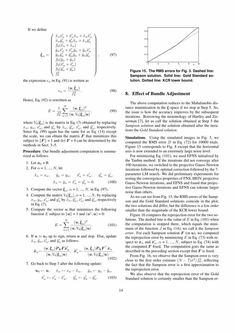
Figure 15. The RMS errors for Fig. 3. Dashed line:Sampson solution. Solid line: Gold Standard so-lution. Dotted line: KCR lower bound.

8. Effect of Bundle Adjustment

The above computation reduces to the Mahalanobis dis-tance minimization in the ξ-space if we stop at Step 5. So,the issue is how the accuracy improves by the subsequentiterations. Borrowing the terminology of Hartley and Zis-serman [7], let us call the solution obtained at Step 5 theSampson solution and the solution obtained after the itera-tions the Gold Standard solution.

Simulations. Using the simulated images in Fig. 3, wecomputed the RMS error D in Eq. (72) for 10000 trials.Figure 15 corresponds to Fig. 8 except that the horizontalaxis is now extended to an extremely large noise level.

For minimizing Eq. (101), we used EFNS initialized bythe Taubin method. If the iterations did not converge after100 iterations, we switched to the projective Gauss-Newtoniterations followed by optimal correction followed by the 7-parameter LM search. We did preliminary experiments fortesting the convergence properties of FNS, HEIV, projectiveGauss-Newton iterations, and EFNS and found that projec-tive Gauss-Newton iterations and EFNS can tolerate largernoise than others.

As we can see from Fig. 15, the RMS errors of the Samp-son and the Gold Standard solutions coincide in the plot;the two solutions did differ, but the difference is a few ordersmaller than the magnitude of the KCR lower bound.

Figure 16 compares the reprojection error for the two so-lutions. The dashed line is the value of E in Eq. (101) whenthe computation is stopped there, which equals the mini-mum of the function J in Eq. (14); we call it the Sampsonerror. For each Sampson solution F (or u), we computedthe reprojection error by minimizing E in Eq. (73) with re-spect to xα and x′

α, α = 1, ..., N , subject to Eq. (74) withthe computed F fixed. The computation goes the same asdescribed in the preceding section except that F is fixed.

From Fig. 16, we observe that the Sampson error is veryclose to the first order estimate (N − 7)σ2/f2

0 , reflectingthe fact that the Sampson error is a first approximation tothe reprojection error.

We also observe that the reprojection error of the GoldStandard solution is certainly smaller than the Sampson er-

14

0

0.001

0.002

0.003

0.004

0.005

0 2 4 6 8 10σ

Figure 16. The reprojection error for Fig. 3.Chained line: Sampson residual. Dashed line:Sampson solution. Solid line: Gold Standard so-lution. Dotted line: (N − 7)σ2/f2

0 .

0

0.1

0.2

0.3

0.4

0 1 2 3 4 5 6 7σ

Figure 17. The RMS errors for Fig. 9. Dashed line:Sampson solution. Solid line: Gold Standard so-lution. Dotted line: KCR lower bound.

0

0.01

0.02

0.03

0 1 2 3 4 5 6 7σ

Figure 18. The reprojection error for Fig. 9.Chained line: Sampson error. Dashed line: Samp-son solution. Solid line: Gold Standard solution.Dotted line: (N − 7)σ2/f2

0 .

ror if the noise level is above a certain level (about 6 pixelsin this case), yet the reprojection error is virtually identicalfor the Sampson and the Gold Standard solutions.

Figures 17 and 18 show the results corresponding toFigs. 15 and 16 for Fig. 9. Again, we observe similar be-havior.

Observations. From our experiments, we conclude that 1)the reprojection is smaller than the Sampson error if thenoise is very large, but that 2) the solution that minimizesthe Sampson error also minimizes the reprojection error,

Figure 19. Real images and 100 correspondingpoints.

Table 1. Residuals and execution times (sec).

method residual timeSVD-corrected LS 45.550 . 00052SVD-corrected ML 45.556 . 00652CFNS 45.556 . 01300opt. corrected ML 45.378 . 007647-LM from LS 45.378 . 011367-LM from opt. corrected ML 45.378 . 01748EFNS 45.379 . 01916bundle adjustment 45.379 . 02580

and vice versa.Let us call the computed fundamental matrix meaningful

if its relative error is less than 50%. Certainly, we cannot ex-pect meaningful applications of camera calibration or 3-Dreconstruction if the computed fundamental matrix has 50%or larger error. We can see that Figs. 15 and 17 nearly cov-ers the noise level range for which meaningful estimation ispossible (recall that the solution is normalized to unit norm,so the RMS error roughly corresponds to the relative error).

If the noise is very large, the objective function becomesvery flat around its minimum, so large deviations are in-evitable whatever computational method is used; the KCRlower bound exactly describes this situation. From sucha wide distribution, we may sometimes observe a solutionvery close to the true value and other times a very wrongone. So, the accuracy evaluation must be done with a largenumber of trials. In fact, we observed that the RMS errorplots of the Sampson and the Gold Standard solutions werevisibly different with 1000 trials for each σ. However, theycoincided after 10000 trials. In the past, a hasty conclusionwas often drawn after a few experiments. Doing many ex-periments, we failed to observe that the Gold Standard solu-tion is any better than the Sampson solution, quite contraryto the assertion by Hartley and Zisserman [7].

Real image example. We manually selected 100 pairs ofcorresponding points in the two images in Fig. 19 and com-puted the fundamental matrix from them. The final resid-ual J and the execution time (sec) are listed in Table 1.We used Core2Duo E6700 2.66GHz for the CPU with 4GBmain memory and Linux for the OS.

We can see that for this example optimally corrected

15

ML, 7-parameter LM (abbr. 7-LM) started from either LSor optimally corrected ML, EFNS, and bundle adjustmentall converged to the same solution, indicating that all areoptimal. For this solution, the reprojection error E numer-ically coincides with the residual J . We can also see thatSVD-corrected LS (Hartley’s 8-point method) and SVD-corrected ML have higher residual than the optimal solutionand that CFNS has as high a residual as SVD-corrected ML.

9. Conclusions

We categorized algorithms for computing the fundamen-tal matrix from point correspondences into “a posteriori cor-rection”, “internal access”, and “external access” and re-viewed existing methods in this framework. Then, we pro-posed new effective schemes10:

1. a new internal access method: 7-parameter LM search.

2. a new external access method: EFNS.

3. a new bundle adjustment algorithm using EFNS.

We conducted experimental comparison and observedthat the popular SVD-corrected LS (Hartley’s 8-point al-gorithm) has poor performance. We also observed that theCFNS of Chojnacki et al. [4], a pioneering external accessmethod, does not necessarily converge to a correct solution,while our EFNS always yields an optimal value; we gave amathematical justification to this.

After many experiments (not all shown here), we con-cluded that EFNS and the 7-parameter LM search startedfrom optimally corrected ML exhibited the best perfor-mance. We also observed that additional bundle adjustment(Gold Standard) does not increase the accuracy to any no-ticeable degree.

Acknowledgments: This work was done in part in collaborationwith Mitsubishi Precision, Co. Ldt., Japan. The authors thankMike Brooks, Wojciech Chojnacki, and Anton van den Hengelof the University Adelaide, Australia, for providing software andhelpful discussions. They also thank Nikolai Chernov of the Uni-versity of Alabama at Birmingham, U.S.A. for helpful discussions.

References[1] A. Bartoli and P. Sturm, Nonlinear estimation of fundamen-

tal matrix with minimal parameters, IEEE Trans. Patt. Anal.Mach. Intell., 26-3 (2004-3), 426–432.

[2] N. Chernov and C. Lesort, Statistical efficiency of curve fit-ting algorithms, Comput. Stat. Data Anal., 47-4 (2004-11),713–728.

[3] W. Chojnacki, M. J. Brooks, A. van den Hengel and D. Gaw-ley, On the fitting of surfaces to data with covariances, IEEETrans. Patt. Anal. Mach. Intell., 22-11 (2000-11), 1294–1303.

10Source codes are available athttp://www.iim.ics.tut.ac.jp/˜sugaya/public-e.html

[4] W. Chojnacki, M. J. Brooks, A. van den Hengel and D. Gaw-ley, A new constrained parameter estimator for computervision applications, Image Vision Comput., 22-2 (2004-2),85–91.

[5] W. Chojnacki, M.J. Brooks, A. van den Hengel, and D. Gaw-ley, FNS, CFNS and HEIV: A unifying approach, J. Math.Imaging Vision, 23-2 (2005-9), 175–183.

[6] R. I. Hartley, In defense of the eight-point algorithm, IEEETrans. Patt. Anal. Mach. Intell., 19-6 (1997-6), 580–593.

[7] R. Hartley and A. Zisserman, Multiple View Geometry inComputer Vision, Cambridge University Press, Cambridge,U.K., 2000.

[8] C. Harris and M. Stephens, A combined corner and edge de-tector, Proc. 4th Alvey Vision Conf., August 1988, Manch-ester, U.K., pp.147–151.

[9] K. Kanatani, Statistical Optimization for Geometric Compu-tation: Theory and Practice, Elsevier Science, Amsterdam,The Netherlands, 1996; Dover, New York, 2005.

[10] K. Kanatani, Ellipse fitting with hyperaccuracy, IEICETrans. Inf. & Sys.,, E89-D-10 (2006-10), 2653–2660.

[11] K. Kanatani and Y. Sugaya, High accuracy fundamentalmatrix computation and its performance evaluation, IEICETrans. Inf. & Syst., E90-D-2 (2007-2), 579–585.

[12] K. Kanatani and Y. Sugaya, Extended FNS for constrainedparameter estimation, Proc. 10th Meeting Image Recog. Un-derstand., July 2007, Hiroshima, Japan, pp. 219–226.

[13] Y. Kanazawa and K. Kanatani Robust image matching pre-serving global consistency, Proc. 6th Asian Conf. Comput.Vision, January 2004, Jeju Island, Korea, Vol. 2, pp. 1128–1133.

[14] Y. Leedan and P. Meer, Heteroscedastic regression in com-puter vision: Problems with bilinear constraint, Int. J. Com-put. Vision, 37-2 (2000-6), 127–150.

[15] D. G. Lowe, Distinctive image features from scale-invariantkeypoints, Int. J. Comput. Vision, 60-2 (2004-11), 91–110.

[16] J. Matei and P. Meer, Estimation of nonlinear errors-in-variables models for computer vision applications, IEEETrans. Patt. Anal. Mach. Intell., 28-10 (2006-10), 1537–1552.

[17] J. Matasu, O. Chum, M. Urban, and T. Pajdla, Robust wide-baseline stereo from maximally stable extremal regions, Im-age Vision Comput., 22-10 (2004-9), 761–767.

[18] K. Mikolajczyk and C. Schmidt, Scale and affine invariantinterest point detectors, Int. J. Comput. Vision, 60-1 (2004-10), 63–86.

[19] P. Meer, Robust techniques for computer vision, in G.Medioni and S. B. Kang (Eds.), Emerging Topics in Com-puter Vision, Prentice Hall, Upper Saddle River, NJ, U.S.A.,2004, pp. 107–190.

[20] T. Migita and T. Shakunaga, One-dimensional search for re-liable epipole estimation, Proc. IEEE Pacific Rim Symp. Im-age and Video Technology, December 2006, Hsinchu, Tai-wan, pp. 1215–1224.

[21] S. M. Smith and J. M. Brady, SUSAN—A new approachto low level image processing, Int. J. Comput. Vision, 23-1(1997-1), pp. 45–78.

[22] Y. Sugaya and K. Kanatani, High accuracy computationof rank-constrained fundamental matrix, Proc. 18th British

16

Machine Vision Conf., September 2007, Coventry, U.K.[23] G. Taubin, Estimation of planar curves, surfaces, and non-

planar space curves defined by implicit equations with appli-cations to edge and range image segmentation, IEEE Trans.Patt. Anal. Mach. Intell., 13-11 (1991-11), 1115–1138.

[24] Z. Zhang, R. Deriche, O. Faugeras and Q.-T. Luong, Arobust technique for matching two uncalibrated imagesthrough the recovery of the unknown epipolar geometry, Ar-tif. Intell., 78 (1995), 87–119.

[25] Z. Zhang and C. Loop, Estimating the fundamental matrixby transforming image points in projective space, Comput.Vision Image Understand., 82-2 (2001-5), 174–180.

Appendix

A. Derivation of the 6-parameter LM

First, note that if F has the form of Eq. (48), we have

‖F ‖2 =3∑

i,j=1

F 2ij = tr[FF>]

= tr[Udiag(σ1, σ2, 0)V>Vdiag(σ1, σ2, 0)U>]= tr[diag(σ2

1 , σ22 , 0)]

= σ21 + σ2

2 , (104)

where we have used the identity tr[AB] = tr[BA] for thematrix trace. Thus, the parameterization of Eqs. (49) en-sures the normalization ‖F ‖ = 1.

Suppose the orthogonal matrices U and V undergo asmall change into U + ∆U and V + ∆V , respectively. Ac-cording to the Lie group theory, there exist small vectors ωand ω′ such that the increments ∆U and ∆V are written as

∆U = ω × U , ∆V = ω′ × V (105)

to a first approximation, where the operator × meanscolumn-wise vector product. Hence, the increment ∆F inF is to a first approximation

∆F = ω × Udiag(cos θ, sin θ, 0)V>

+Udiag(− sin θ∆θ, cos θ∆θ, 0)V>

+Udiag(cos θ, sin θ, 0)(ω′ × V)>. (106)

Taking out the elements, we can rearrange this in the vectorform

∆u = F Uω + uθ∆θ + F V ω′, (107)

where F U and F V are the matrices in Eqs. (51) and uθ isdefined by Eq. (53). The resulting increment ∆J in J iswritten to a first approximation

∆J = (∇uJ,∆u) = (2Xu, F Uω + uθ∆θ + F V ω′)

= 2(F>Xu,ω) + 2(uθ, Xu)∆θ + 2(F V XuJ,ω′),(108)

which shows that the first derivatives of J are given byEqs. (50) and (52). If we further change u into u + ∆u

in the above expression, we have to a first approximation(i.e., up to the second order in ∆u),

∆2J = (∆u,∇2uJ∆u)

= (F Uω+uθ∆θ+F V ω′, 2M(F Uω+uθ∆θ+F V ω′))

= 2(ω, F>UMF Uω) + 2(ω′, F>

V MF V ω′)

+2(uθ, Muθ)∆θ2 + 4(ω, F>UMω′)

+4(ω, F>UMuθ)∆θ + 4(ω′, F>

V Muθ)∆θ, (109)

where we have used the Gauss-Newton approximation ∇2uJ

≈ 2M . From this, we obtain the second derivatives inEqs. (54).

B. Details of CFNS

According to Chojnacki et al. [4], the matrix Q used inEq. (63) is given, without any background reasoning, as fol-lows (their original symbols are somewhat altered to con-form to the use in this paper).

The gradient ∇uJ = (∂J/∂ui) and the Hessian ∇2uJ =

(∂2J/∂ui∂uj) of the function J in Eq. (14) are

∇uJ = 2(M − L)u, ∇2uJ = 2(M − L) − 8(S − T ),

(110)where M and L are the matrices in Eqs. (22), and we define

S =N∑

α=1

(u, ξα)S[ξα(V0[ξα]u)>](u, V0[ξα]u)2

,

T =N∑

α=1

(u, ξα)2(V0[ξα]u)(V0[ξα]u>)>

(u, V0[ξα]u)3. (111)

Here, S[ · ] is the symmetrization operator (S[A] = (A +A>)/2). Let

A = P u†(∇2uJ)(2uu> − I),

B =2

‖ detu‖

( 9∑i=1

S[((∇2u det u)ei)u†>](∇uJ)e>

i

−(u†,∇uJ)u†u†>∇2u det u

),

C = 3( detu

‖∇u detu‖2∇2

u det u

+u†u†>(I − 2 detu

‖∇u detu‖2∇2

u det u))

, (112)

where u† is the vector in Eq. (9), P u† is the projection ma-trix in Eq. (59), and ei is the ith coordinate basis vector(with 0 components except 1 in the ith position). The ma-trix Q is given by

Q = (A + B + C)(A + B + C)>. (113)

17

C. Details of bundle adjustment

Introducing Lagrange multipliers λα, µα, and µ′α for the

constraints of Eqs. (78), and (79) to Eq. (76), we let

L =N∑

α=1

(‖∆xα‖2 + ‖∆x′

α‖2)

−N∑

α=1

λα

((Fx′

α, ∆xα) + (F>xα,∆x′α)

)−

N∑α=1

µα(k, ∆xα) −N∑

α=1

µ′α(k, ∆x′

α). (114)

Putting the derivatives of L with respect to ∆xα and ∆x′α

to 0, we have

2∆xα − λαFx′α − µαk = 0,

2∆x′α − λαF>xα − µ′

αk = 0. (115)

Multiplying the projection matrix P k in Eq. (81) on bothsides from left and noting that P k∆xα = ∆xα, P k∆x′

α =∆x′

α, and P kk = 0, we have

2∆xα − λαP kFx′α = 0, 2∆x′

α − λαP kF>xα = 0.(116)

Hence, we obtain

∆xα =λα

2P kFx′

α, ∆x′α =

λα

2P kF>xα. (117)

Subsitituting these into Eq. (78), we have

(Fx′α,

λα

2P kFx′

α)+(F>xα,λα

2P kF>xα)=(xα,Fx′

α),(118)

and hence

λα

2=

(xα, Fx′α)

(Fx′α,P kFx′

α) + (F>xα, P kF>xα). (119)

Substituting this into Eq. (117), we obtain Eqs. (80). If wesubstitute Eqs. (80) into Eq. (76), we have

E =N∑

α=1

(∥∥∥∥ (xα, Fx′α)P kFx′

α

(x′α,F>P kFx′

α) + (xα, FP kF>xα)

∥∥∥∥2

+

∥∥∥∥∥ (xα, Fx′α)P kF>xα

(x′α, F>P kFx′

α) + (xα,FP kF>xα)

∥∥∥∥∥2)

=N∑

α=1

(xα, Fx′α)2(‖P kFx′

α‖2 + ‖P kF>xα‖2)((Fx′

α,P kFx′α) + (F>xα, P kF>xα)

)2

=N∑

α=1

(xα,Fx′α)2

(Fx′α,P kFx′

α)+(F>xα,P kF>xα), (120)

where we have noted due to the identity P 2k = P k that

‖P kFx′α‖2 = (P kFx′

α, P kFx′α) = (Fx′

α,P 2kFx′

α) =(Fx′

α, P kFx′α). Similarly, we have ‖P kF>xα‖2 =

(F>xα,P kF>xα).Introducing Lagrange multipliers λα, µα, and µ′

α for theconstraints of Eqs. (87), and (89) to Eq. (76), we let

L =N∑

α=1

(‖xα + ∆xα‖2 + ‖x′

α + ∆x′α‖2

)−

N∑α=1

λα

((F x′

α,∆xα) + (F>xα,∆x′α)

)−

N∑α=1

µα(k, ∆xα) −N∑

α=1

µ′α(k, ∆x′

α). (121)

Putting the derivatives of L with respect to ∆xα and ∆x′α

to 0, we have

2(xα + ∆xα) − λαF x′α − µαk = 0,

2(x′α + ∆x′

α) − λαF>xα − µ′αk = 0. (122)

Multiplying P k on both sides from left, we have

2xα + 2∆xα − λαP kF x′α = 0,

2xα + 2∆x′α − λαP kF>xα = 0. (123)

Substituting these into Eq. (88), we have

∆xα =λα

2P kF x′

α − xα, ∆x′α =

λα

2P kF>xα − x′

α.

(124)Subsitituting these into Eq. (88), we obtain

(F x′α,

λα

2P kF x′

α − xα)

+(F>xα,λα

2P kF>xα − x′

α) = (xα, F x′α), (125)

and hence

λα

2=

(xα,F x′α) + (F x′

α, xα) + (F>xα, x′α)

(F x′α,P kF x′

α) + (F>xα, P kF>xα). (126)

Subsitituting this into Eq. (124), we obtain Eq. (92). If wesubstitute Eq. (92) into Eq. (85), we have

E =N∑

α=1

(∥∥∥∥ eαP kF x′α

(F x′α, P kF x′

α) + (F>xα,P kF>xα)

∥∥∥∥2

+

∥∥∥∥∥ eαP kF>xα

(F x′α, P kF x′

α) + (F>xα, P kF>xα)

∥∥∥∥∥2)

=N∑

α=1

e2α(‖P kF x′

α‖2 + ‖P kF>xα‖2)((F x′

α, P kF x′α) + (F>xα, P kF>xα)

)2

=N∑

α=1

e2α

(F x′α, P kF x′

α) + (F>xα, P kF>xα). (127)

18