Optimal Partitioning for Parallel Matrix Computation on a Small Number of Abstract Heterogeneous Processors Ashley DeFlumere UCD Student Number: 10286438 This thesis is submitted to University College Dublin in fulfilment of the requirements for the degree of Doctor of Philosophy in Computer Science School of Computer Science and Informatics Head of School : P´adraig Cunningham Research Supervisor: Alexey Lastovetsky September 2014

Welcome message from author
This document is posted to help you gain knowledge. Please leave a comment to let me know what you think about it! Share it to your friends and learn new things together.
Transcript
Optimal Partitioning for Parallel MatrixComputation on a Small Number of Abstract
Heterogeneous Processors
Ashley DeFlumereUCD Student Number: 10286438
This thesis is submitted to University College Dublin infulfilment of the requirements for the degree of
Doctor of Philosophy in Computer Science
School of Computer Science and Informatics
Head of School : Padraig Cunningham
Research Supervisor: Alexey Lastovetsky
September 2014
Contents
1 Introduction to Heterogeneous Computing and Data Parti-tioning 11.1 Heterogeneous Computing . . . . . . . . . . . . . . . . . . . . 2
1.1.1 Types of Heterogeneous Systems . . . . . . . . . . . . 21.1.2 Benefits of Heterogeneity . . . . . . . . . . . . . . . . . 31.1.3 Issues in Heterogeneous Computing . . . . . . . . . . . 3
1.2 Dense Linear Algebra and Matrix Computation . . . . . . . . 41.3 Data Partitioning . . . . . . . . . . . . . . . . . . . . . . . . . 51.4 The Optimal Data Partition Shape Problem . . . . . . . . . . 6
1.4.1 Defining Optimality . . . . . . . . . . . . . . . . . . . . 61.4.2 Problem Formulation . . . . . . . . . . . . . . . . . . . 71.4.3 Roadmap to the Optimal Shape Solution . . . . . . . . 7
1.5 Contributions of this Thesis . . . . . . . . . . . . . . . . . . . 8
2 Background and Related Work 92.1 A Brief Review of Matrix Multiplication . . . . . . . . . . . . 9
2.1.1 Basic Matrix Multiplication . . . . . . . . . . . . . . . 92.1.2 Parallel Matrix Multiplication . . . . . . . . . . . . . . 10
2.2 Rectangular Data Partitioning . . . . . . . . . . . . . . . . . . 132.2.1 One-Dimensional Partitioning . . . . . . . . . . . . . . 132.2.2 Two-Dimensional Partitioning . . . . . . . . . . . . . . 142.2.3 Performance Model Based Partitioning . . . . . . . . . 16
2.3 Non-Rectangular Data Partitioning . . . . . . . . . . . . . . . 162.3.1 Two Processors . . . . . . . . . . . . . . . . . . . . . . 162.3.2 Three Processors . . . . . . . . . . . . . . . . . . . . . 17
2.4 Abstract Processors . . . . . . . . . . . . . . . . . . . . . . . . 18
3 Modelling Matrix Computation on Abstract Processors 203.1 Communication Modelling . . . . . . . . . . . . . . . . . . . . 21
3.1.1 Fully Connected Network Topology . . . . . . . . . . . 223.1.2 Star Network Topology . . . . . . . . . . . . . . . . . . 22
i
3.2 Computation Modelling . . . . . . . . . . . . . . . . . . . . . 233.3 Memory Modelling . . . . . . . . . . . . . . . . . . . . . . . . 243.4 Algorithm Description . . . . . . . . . . . . . . . . . . . . . . 25
3.4.1 Bulk Communication with Barrier Algorithms . . . . . 253.4.2 Communication/Computation Overlap Algorithms . . 27
4 The Push Technique 294.1 General Form . . . . . . . . . . . . . . . . . . . . . . . . . . . 294.2 Using the Push Technique to solve the Optimal Data Partition
Shape Problem . . . . . . . . . . . . . . . . . . . . . . . . . . 314.3 Application to Matrix Multiplication . . . . . . . . . . . . . . 324.4 Push Technique on a Two Processor System . . . . . . . . . . 32
4.4.1 Algorithmic Description . . . . . . . . . . . . . . . . . 334.4.2 Push: Lowering Communication Time for all Algorithms 344.4.3 Two Processor Optimal Candidates . . . . . . . . . . . 36
5 Two Processor Optimal Partition Shape 395.1 Optimal Candidates . . . . . . . . . . . . . . . . . . . . . . . 395.2 Applying the Abstract Processor Model . . . . . . . . . . . . . 415.3 Optimal Two Processor Data Partition . . . . . . . . . . . . . 475.4 Experimental Results . . . . . . . . . . . . . . . . . . . . . . . 52
5.4.1 Experimental Setup . . . . . . . . . . . . . . . . . . . . 525.4.2 Results by Algorithm . . . . . . . . . . . . . . . . . . . 53
6 The Push Technique Revisited: Three Processors 596.1 Additional Push Constraints . . . . . . . . . . . . . . . . . . . 596.2 Implementing the Push DFA . . . . . . . . . . . . . . . . . . . 61
6.2.1 Motivation . . . . . . . . . . . . . . . . . . . . . . . . . 616.2.2 Algorithmic Description . . . . . . . . . . . . . . . . . 626.2.3 End Conditions . . . . . . . . . . . . . . . . . . . . . . 63
6.3 Experimental Results with the Push DFA . . . . . . . . . . . 636.3.1 Experimental Setup . . . . . . . . . . . . . . . . . . . . 636.3.2 Description of Shape Archetypes . . . . . . . . . . . . 656.3.3 Reducing All Other Archetypes to Archetype A . . . . 67
6.4 Push Technique on Four or More Processors . . . . . . . . . . 72
7 Three Processor Optimal Partition Shape 747.1 Archetype A: Candidate Shapes . . . . . . . . . . . . . . . . . 74
7.1.1 Formal Definition of Candidate Shapes . . . . . . . . . 757.1.2 Finding the Canonical Version of each Shape . . . . . . 77
7.2 Network Topology Considerations . . . . . . . . . . . . . . . . 80
ii
7.3 Fully Connected Network Topology . . . . . . . . . . . . . . . 817.3.1 Pruning the Optimal Candidates . . . . . . . . . . . . 817.3.2 Optimal Three Processor FC Data Partition . . . . . . 847.3.3 Experimental Results . . . . . . . . . . . . . . . . . . . 95
7.4 Star Network Topology . . . . . . . . . . . . . . . . . . . . . . 987.4.1 Pruning the Optimal Candidates . . . . . . . . . . . . 987.4.2 Applying the Abstract Processor Model . . . . . . . . . 997.4.3 Optimal Three Processor ST Data Partition . . . . . . 105
7.5 Conclusion . . . . . . . . . . . . . . . . . . . . . . . . . . . . . 114
8 Local Search Optimisations 1158.1 Description of Local Search . . . . . . . . . . . . . . . . . . . 1158.2 Simulated Annealing . . . . . . . . . . . . . . . . . . . . . . . 115
8.2.1 Experimental Method for Matrix Partitioning . . . . . 1168.3 Conclusion . . . . . . . . . . . . . . . . . . . . . . . . . . . . . 117
9 The Push Technique and LU Factorisation 1199.1 A Brief Review of LU Factorisation . . . . . . . . . . . . . . . 119
9.1.1 Basic LU Factorisation . . . . . . . . . . . . . . . . . . 1199.1.2 Parallel LU Factorisation . . . . . . . . . . . . . . . . . 120
9.2 Background on Data Partitioning for LU Factorisation . . . . 1219.2.1 One-Dimensional Partitioning . . . . . . . . . . . . . . 1219.2.2 Two-Dimensional Partitioning . . . . . . . . . . . . . . 123
9.3 Applying Push to LU Factorisation . . . . . . . . . . . . . . . 1239.3.1 Special Considerations of LU Push . . . . . . . . . . . 1249.3.2 Methodology of LU Push . . . . . . . . . . . . . . . . . 1249.3.3 Two Processor Optimal Candidates . . . . . . . . . . . 125
10 Further Work 12710.1 Arbitrary Number of Processors . . . . . . . . . . . . . . . . . 12710.2 Increasing Complexity of Abstract Processor . . . . . . . . . . 128
10.2.1 Non-Symmetric Network Topology . . . . . . . . . . . 12810.2.2 Computational Performance Model . . . . . . . . . . . 12810.2.3 Memory Model . . . . . . . . . . . . . . . . . . . . . . 129
10.3 Push Technique and Other Matrix Computations . . . . . . . 129
11 Conclusions 13011.1 The Push Technique . . . . . . . . . . . . . . . . . . . . . . . 13011.2 Non-Rectangular Partitioning . . . . . . . . . . . . . . . . . . 131
11.2.1 The Square Corner Shape . . . . . . . . . . . . . . . . 13111.2.2 The Square Rectangle Shape . . . . . . . . . . . . . . . 132
iii
11.3 Pushing the Boundaries: Wider Applicability . . . . . . . . . . 133
A Two Processor Push Algorithmic Description 134A.1 Push Down . . . . . . . . . . . . . . . . . . . . . . . . . . . . 134A.2 Push Up . . . . . . . . . . . . . . . . . . . . . . . . . . . . . . 135A.3 Push Over . . . . . . . . . . . . . . . . . . . . . . . . . . . . . 136A.4 Push Back . . . . . . . . . . . . . . . . . . . . . . . . . . . . . 136
B Push Lowers Communication Time: Two Processor Proofs 138B.1 Serial Communication . . . . . . . . . . . . . . . . . . . . . . 138B.2 Parallel Communication . . . . . . . . . . . . . . . . . . . . . 139B.3 Canonical Forms . . . . . . . . . . . . . . . . . . . . . . . . . 141
C Push Lowers Execution Time: Three Processor Proofs 142C.1 Serial Communication with Barrier . . . . . . . . . . . . . . . 142C.2 Parallel Communication with Barrier . . . . . . . . . . . . . . 143C.3 Serial Communication with Bulk Overlap . . . . . . . . . . . . 143C.4 Parallel Communication with Overlap . . . . . . . . . . . . . . 144C.5 Parallel Interleaving Overlap . . . . . . . . . . . . . . . . . . . 144
D Three Processor Fully Connected Optimal Shape Proofs 145D.1 Serial Communication with Overlap . . . . . . . . . . . . . . . 145
D.1.1 Square Corner Description . . . . . . . . . . . . . . . . 145D.1.2 SCO Optimal Shape . . . . . . . . . . . . . . . . . . . 150
D.2 Parallel Communication with Overlap . . . . . . . . . . . . . . 152D.2.1 Square Corner . . . . . . . . . . . . . . . . . . . . . . . 152D.2.2 Square Rectangle . . . . . . . . . . . . . . . . . . . . . 154D.2.3 Block Rectangle . . . . . . . . . . . . . . . . . . . . . . 155D.2.4 PCO Optimal Shape . . . . . . . . . . . . . . . . . . . 155
iv
List of Figures
2.1 Basic Matrix Multiplication . . . . . . . . . . . . . . . . . . . 102.2 Parallel Matrix Multiplication . . . . . . . . . . . . . . . . . . 122.3 One Dimensional Partitions . . . . . . . . . . . . . . . . . . . 142.4 Grid and Cartesian Partitioning . . . . . . . . . . . . . . . . . 152.5 Column Based Partitioning . . . . . . . . . . . . . . . . . . . 152.6 Previous Two Processor Non-Rectangular Work . . . . . . . . 172.7 Previous Three Processor Non-Rectangular Work . . . . . . . 172.8 Example of Hybrid CPU/GPU System . . . . . . . . . . . . . 19
3.1 Fully Connected Network Topology . . . . . . . . . . . . . . . 233.2 Star Network Topology . . . . . . . . . . . . . . . . . . . . . . 233.3 Communication Pattern for Square Corner . . . . . . . . . . . 253.4 Serial and Parallel Communication with Barrier Algorithm
Description . . . . . . . . . . . . . . . . . . . . . . . . . . . . 263.5 Serial and Parallel Communication with Overlap Algorithm
Description . . . . . . . . . . . . . . . . . . . . . . . . . . . . 27
4.1 Example of Enclosing Rectangles . . . . . . . . . . . . . . . . 304.2 Example of Two Processor Push in all Directions . . . . . . . 344.3 Two Processor Push DFA Results . . . . . . . . . . . . . . . . 37
5.1 Two Processor MMM Optimal Candidates . . . . . . . . . . . 405.2 Communication Pattern for Square Corner . . . . . . . . . . . 415.3 Two Processor Square Corner portion for overlap . . . . . . . 425.4 Two Processor SCO Square Corner constituent functions of
Texe max . . . . . . . . . . . . . . . . . . . . . . . . . . . . . . 445.5 Two Processor PCO Square Corner constituent functions of
Texe max . . . . . . . . . . . . . . . . . . . . . . . . . . . . . . 465.6 Two Processor SCB Theoretical Curves . . . . . . . . . . . . . 535.7 Two Processor SCB Experimental Curves . . . . . . . . . . . 545.8 Two Processor PCB Theoretical Curves . . . . . . . . . . . . . 545.9 Two Processor PCB Experimental Curves . . . . . . . . . . . 55
v
5.10 Two Processor SCO Experimental Curves r < 3 . . . . . . . . 555.11 Two Processor SCO Experimental Curves r > 3 . . . . . . . . 565.12 Two Processor PCO Experimental Curves r < 3 . . . . . . . . 575.13 Two Processor PCO Experimental Curves r > 3 . . . . . . . . 575.14 Two Processor PIO Experimental Curves - Computation dom-
inant . . . . . . . . . . . . . . . . . . . . . . . . . . . . . . . . 585.15 Two Processor PIO Experimental Curves - Communication
dominant . . . . . . . . . . . . . . . . . . . . . . . . . . . . . 58
6.1 Push DFA State Diagram Example . . . . . . . . . . . . . . . 646.2 Three Processor DFA Results - All Archetypes . . . . . . . . . 666.3 Introduction to Corners . . . . . . . . . . . . . . . . . . . . . 686.4 Taxonomy of Corner Labels . . . . . . . . . . . . . . . . . . . 696.5 Three Processor Archetype B Shapes . . . . . . . . . . . . . . 70
7.1 Six Candidates of Archetype A - General Form . . . . . . . . . 757.2 Two Versions of Type One Partition . . . . . . . . . . . . . . 787.3 Three Processor Candidate Shapes - Canonical Form . . . . . 797.4 Three Processor Fully Connected Network Topology . . . . . . 807.5 Three Processor Star Network Topology . . . . . . . . . . . . 807.6 Three Processor Rectangle Corner and Block Rectangle Canon-
ical Form . . . . . . . . . . . . . . . . . . . . . . . . . . . . . 827.7 Three Processor L Rectangle Partition Shape Canonical Form 837.8 Three Processor SCB 3D Graph . . . . . . . . . . . . . . . . . 877.9 Three Processor PCB 3D Graph . . . . . . . . . . . . . . . . . 897.10 Three Processor SCO 3D Graph . . . . . . . . . . . . . . . . . 927.11 Three Processor PCO 3D Graph . . . . . . . . . . . . . . . . . 937.12 Three Processor SCB Experimental Results . . . . . . . . . . 967.13 Three Processor PCB Experimental Results . . . . . . . . . . 977.14 Three Processor Star Topology Candidate Shapes . . . . . . . 997.15 Three Processor Star Topology Variant One 3D Graph Serial
Communication . . . . . . . . . . . . . . . . . . . . . . . . . . 1077.16 Three Processor Star Topology Variant One 3D Graph Parallel
Communication . . . . . . . . . . . . . . . . . . . . . . . . . . 1087.17 Three Processor Star Topology Variant Two 3D Graph Serial
Communication . . . . . . . . . . . . . . . . . . . . . . . . . . 1107.18 Three Processor Star Topology Variant Two 3D Graph Paral-
lel Communication . . . . . . . . . . . . . . . . . . . . . . . . 1117.19 Three Processor Star Topology Variant Three 3D Graph Serial
Communication . . . . . . . . . . . . . . . . . . . . . . . . . . 112
vi
7.20 Three Processor Star Topology Variant Three 3D Graph Par-allel Communication . . . . . . . . . . . . . . . . . . . . . . . 113
8.1 Simulated Annealing Results Unpermuted . . . . . . . . . . . 1178.2 Simulated Annealing Results Permuted . . . . . . . . . . . . . 118
9.1 LU factorisation parallel algorithm . . . . . . . . . . . . . . . 1229.2 LU Factorisation One-Dimensional Partition Shape . . . . . . 1239.3 LU Factorisation Two-Dimensional Partition Shape . . . . . . 1249.4 Push for LU Factorisation . . . . . . . . . . . . . . . . . . . . 1259.5 Push for LU Factorisation . . . . . . . . . . . . . . . . . . . . 1269.6 Some LU Factorisation Candidates . . . . . . . . . . . . . . . 126
11.1 Square Corner Optimal Shape . . . . . . . . . . . . . . . . . . 13111.2 Square Rectangle Optimal Shape . . . . . . . . . . . . . . . . 132
D.1 Overlap Area of Square Corner for SCO and PCO Algorithms 146D.2 Three Processor SCO Square Corner . . . . . . . . . . . . . . 149
vii
Abstract
High Performance Computing (HPC) has grown to encompass many newarchitectures and algorithms. The Top500 list, which ranks the world’sfastest supercomputers every six months, shows this trend towards a va-riety of heterogeneous architectures - particularly multicores and generalpurpose Graphical Processing Units (GPUs). Heterogeneity, whether it isin computational power or communication interconnect, provides new chal-lenges in programming and algorithm development. The general trend hasbeen to adapt algorithms used on homogeneous parallel systems for use inthe new heterogeneous parallel systems. However, assumptions carried overfrom those homogeneous systems are not always applicable to heterogeneoussystems.
Linear algebra matrix operations are widely used in scientific computingand are an area of significant HPC study. To parallelise matrix operationsover many nodes in an HPC system, each processor is given a section of thematrix to compute. These sections are collectively called the data partition.Linear algebra operations, such as matrix matrix multiplication (MMM) andLU factorisation, use data partitioning based on the original homogeneousalgorithms. Specifically, each processor is assigned a rectangular sub matrix.The primary motivation of this work is to question whether the rectangulardata partitioning is optimal for heterogeneous systems.
This thesis will show the rectangular data partitioning is not universallyoptimal when applied to the heterogeneous case. The major contributionwill be a new method for creating optimal data partitions, called the PushTechnique. This method is used to make small, incremental changes to adata partition, while guaranteeing not to worsen it. The end result is a smallnumber of potentially optimal data partitions, called candidates. These can-didates are then analysed for differing numbers of processors and topologies.The validity of the Push Technique is verified analytically and experimen-tally.
The optimal data partition for matrix operations is found for systems oftwo and three heterogeneous processors, including differing communicationtopologies. A methodology is outlined for applying the Push Technique tomatrix computations other than MMM, such as LU Factorisation, and forlarger numbers of heterogeneous processors.

Statement of OriginalAuthorship
I hereby certify that the submitted work is my own work, was completedwhile registered as a candidate for the degree stated on the Title Page, and Ihave not obtained a degree elsewhere on the basis of the research presentedin this submitted work.
viii
Acknowledgements
First and foremost I must extend my utmost gratitude to my supervisor,Alexey Lastovetsky. I couldn’t imagine a better research advisor. Thankyou for teaching me so much about thinking and writing like a scientist, butmost importantly, thank you for teaching me how to balance work and lifeto become a happier person.
Thank you to my examiners, Umit Catalyurek and Neil Hurley, for theirhelpful corrections and support.
This thesis is the result of research conducted with the financial supportof Science Foundation Ireland under Grant Number 08/IN./I2054. Experi-ments were carried out on Grid’5000 developed under the INRIA ALADDINdevelopment action with support from CNRS, RENATER and several Uni-versities as well as other funding bodies (see https://www.grid5000.fr).
I am very grateful for the opportunity to travel to INRIA in Bordeaux,France to work with the wonderful Olivier Beaumont, which was fundedby COST Action IC0805 “Open European Network for High PerformanceComputing on Complex Environments”.
I owe a huge debt of gratitude to my eternal proof-reader and calculation-checker, my father, Michael DeFlumere.
Thank you to Sadaf Alam for introducing me to research at Oak Ridge,and encouraging me to pursue a graduate degree (and to consider doing sooutside the USA!). I would also like to thank the Department of ComputerScience at Mount Holyoke College, especially Barbara Lerner, Paul Dobosh,and Jim Teresco, for their unfailing encouragement during my time there.
Thank you to the members of the Heterogeneous Computing Lab, VladimirRychkov, David Clarke, Kiril Dichev, Ziming Zhong, Ken O’Brien, Tania Ma-lik, Khalid Hasanov, Oleg Girko, and Amani Al Onazi. A very special thanksto Brett Becker for getting me started on the Square Corner.
To my family, my friends, and all my teammates at Ireland Lacrosse,thank you for supporting me and my crazy dreams.
And finally, I would like thank my cat for tolerating a transatlantic jour-ney to be my constant companion and the keeper of my sanity.
ix

For Dr. Richard Edward Mulcahy(1913 - 2003)
x
Chapter 1
Introduction to HeterogeneousComputing and DataPartitioning
The world of High Performance Computing (HPC) has grown to encompassmany new architectures, algorithms, models and tools. Over the past fourdecades, HPC systems, comprised of increasingly complex and numerouscomponents, have grown by orders of magnitude in terms of computationalpower, as measured by the number of floating point operations per second(FLOPs).
As machines increased in size and parallelism, the teraFLOP barrier wasreached in 1996 by the ASCI Red supercomputer [1]. Just over a decadelater, the petaFLOP barrier was broken by the Roadrunner supercomputerin 2008 [2].
The Top5001 list [3], which ranks the world’s fastest computers everysix months, clearly shows a trend towards a variety of heterogeneous archi-tectures - particularly multicores and hardware accelerators such as GPUs(Graphical Processing Units)[4, 5]. As of the June 2014 list, 37 systemsaround the world had achieved petaFLOP speeds.
In the coming decade, a monumental effort will be made to achieve exas-cale (1000 petaFLOPs, or 1018 FLOPs) computing systems. The massivelyparallel nature of HPC has led to many new advancements in algorithms,models and tools, which strive to reach the exascale goal by utilising andworking with the latest computer hardware [6]. The software stack, e.g.compilers, message passing, and operating systems, is constantly being up-dated to reflect the new capabilities in performance of both the computation,
1http://www.top500.org
1
and the communication, of new chipsets. In general, as machines becomeheterogeneous in computation and communication the homogeneous parallelalgorithms are adapted for use in these newer systems. However, the impor-tant question remains, what if assumptions carried over from homogeneoussystems are no longer applicable when using a heterogeneous system?
1.1 Heterogeneous Computing
Heterogeneous (adj.) - “Diverse in character or content”-Oxford English Dictionary
In terms of computing, “heterogeneous” refers to non-uniformity in someaspect of the system, either by design or through ageing. In general terms,heterogeneity in computing manifests in three ways:
• differing amounts of computational power among subsystems
• differing amounts of bandwidth or latency within the communicationinterconnect
• some combination of the above two
This may occur naturally as systems age, and begin to be replaced piecemeal.This type of heterogeneity happens particularly in smaller clusters, wherefinancial considerations might preclude an older system from being removedentirely. Heterogeneity is increasingly intentional in HPC, however, withsystems that combine traditional multi-core processors with general purposeGPUs and other hardware accelerators and coprocessors.
1.1.1 Types of Heterogeneous Systems
The following is an incomplete list, but should serve as an example of themany types of heterogeneity in HPC.
• Compute nodes comprised of combinations of CPUs, GPUs, FPGAs(field programmable gate arrays), or coprocessors
• Compute nodes comprised of specialised cores, each tailored to a spe-cific function
• Communication networks with differing bandwidth or latency betweennodes, either symmetric or non-symmetric
2
• Clusters comprised of heterogeneous nodes, or several differing clustersof homogeneous nodes used in concert
• Groups of workstations, often of different computational power, clockfrequency, and system software, used in concert
Whatever the form, heterogeneous systems share the common thread ofnon-uniformity, which has both benefits and drawbacks [7]. These are dis-cussed in the following sections.
1.1.2 Benefits of Heterogeneity
Heterogeneous computing presents many benefits, the scale and scope ofwhich depend largely on the type of heterogeneity present.
The primary benefit of concern in this thesis is increased computationalpower, increasing the data throughput over traditional CPU only systems.GPUs, for instance, were first used to render images in video games, and so,are plentiful and inexpensive compared to other technology available for HPC[8, 9]. The relative computational power of the GPU, specifically for highlydata parallel computations, allows speedups in many scientific applications[10, 11].
Another example of increased computational power, is collection of net-worked workstations viewed as a single HPC system. These workstationsgroups are a network of vastly different computing resources being harnessedfor use on a single problem. This has also been shown to provide computa-tional speedup for linear algebra applications [12, 13].
Other types of heterogeneous systems, can be used to generate benefitsother than increased computational power. Nodes with heterogeneous spe-cialised cores, similar to what has long been used in mobile phones, can beused to increase power efficiency [14, 15]. A general purpose CPU must be ca-pable of a wide variety of tasks, but is not optimised for any of them. Instead,the idea is to orchestrate a variety of specialised heterogeneous resources toaccomplish the same tasks, in a faster and more efficient way [16].
1.1.3 Issues in Heterogeneous Computing
Despite the advantages, heterogeneous systems do present unique challengesin scalability, algorithm development, and programmability for parallel pro-cessing. A GPU, for instance, must be controlled by a CPU core, and haslimited bandwidth for communication and memory access [17].
3
Algorithms which have been carefully tuned for homogeneous parallelsystems must be rethought to provide the optimal performance on hetero-geneous systems, often to take advantage of the increased computationalpower. A large number of proposals have been made for algorithms [18, 19],models [20], and tools [21, 22, 23], to make up this gap in knowledge forheterogeneous systems.
Despite all this prior work, however, HPC systems can be large, complexand difficult to use in an optimal way. This is a rich and open researcharea; how to optimally model and program for these diverse, large scaleheterogeneous environments.
1.2 Dense Linear Algebra and Matrix Com-
putation
Linear algebra operations are widely used in scientific computing and arean important part of HPC. Software packages such as High PerformanceLinPACK (HPL) [24] and ScaLAPACK [25] provide linear algebra imple-mentations for HPC.
Dense linear algebra is essential to the computation of matrices used ina variety of scientific fields. Some fundamental linear algebra kernels, suchas LU factorisation and its underlying parallel computation, matrix multi-plication, are used to solve systems of linear equations with arbitrarily largenumbers of variables. In that way, any scientific field which can approximateits applications by linear equations, such as astronomy, meteorology, physics,and chemistry, can use HPC systems and the ScaLAPACK package to vastlyimprove the execution time of the domain code.
These linear algebra kernels are computationally intense, but often thiscomputational load may be parallelised over many compute nodes. However,this introduces the problem of communicating between the nodes to sharedata and synchronise calculations. As HPC continues to gain computationalpower, the effect of this communication time will grow proportionately [26].
Because of their usefulness in such a wide variety of applications bothmatrix multiplication and LU factorisation have been studied in great detail.Ways to model heterogeneous systems, and algorithms to improve utilisationof computation and communication resources, are being developed and im-proved upon. A full accounting of the advancements in parallel computationof matrix multiplication is given in Chapter 2.
4
1.3 Data Partitioning
A data partition defines the way in which the linear algebra matrices aredivided amongst the available processing resources. Data partitions are gen-erally designed in order to optimise some fundamental metric of the appli-cation, such as execution time, or power efficiency. This thesis will focus onthe former; the overall execution time of the matrix computation.
Data partitions endeavour to optimally distribute the computational loadof the problem matrices amongst the available processors. The speed at whichan individual processor can perform basic operations, like add and multiply,determines the proportion of the overall problem it will be assigned. In thisway, when computing in parallel, all processors will complete computationat the same time, and no processor will sit idle without work.
The other consideration of a data partition is its shape. The shape of adata partition is the location within the matrix of each processor’s assignedportion. In the case of matrix multiplication, the shape of the data parti-tion does not affect the volume of computation (although the cost may beadversely affected by physical constraints such as cache misses dependingon the data types used). However the partition shape does directly affectthe volume of communication. A processor may require data “owned” by asecond processor in order to compute its assigned portion.
In the case of LU factorisation, the layout of processor data within thepartition affects both computation and communication costs. As the fac-torisation proceeds, an increasing amount of the matrix is completed and nolonger used. If the data partition assigns a processor to a section completedearly on, then it will sit idle for the remainder of the execution time; this isclearly inefficient.
The communication time of a data partition is increasingly importantas HPC systems become ever more computationally efficient [26]. A vari-ety of advances have been made in minimising communication for matrixcomputations on heterogeneous systems [27]. The general shapes of thesepartitionings are, however, always rectangular. These are described in detailin Chapter 2.
However, these approaches are fundamentally limited by nature of the factthat they are based on algorithms and techniques developed for homogeneoussystems. To find an optimal solution to the data partition shape problem,one must consider not only rectangular shapes, but all shapes, i.e. non-rectangular.
5
1.4 The Optimal Data Partition Shape Prob-
lem
Despite all the previous study on data partitioning discussed in Chapter2, the problem of optimal data partitioning for heterogeneous processorshas yet to be solved. Finding simply the optimal rectangular shape is NP -complete [28], and research has focused almost exclusively on approximatingthe optimal rectangular solution. The previous work, discussed in Section2.3, studying non-traditional shapes was not concerned with optimality, butwith a direct comparison between one type of rectangular partition and onetype of non-rectangular partition.
The goal of this work is to define, and solve, the broader problem ofoptimality. It is this fundamental broadness that necessitates a focus onsmall numbers of heterogeneous processors. This is a natural starting placefor the larger problem of optimal data partitioning on arbitrary numbersof heterogeneous processors. The remainder of this section sets out the re-search questions and aims, and provides a roadmap of how the optimal datapartition shape problem will be solved.
1.4.1 Defining Optimality
Optimal (adj.) - “Best or most favourable; optimum”- Oxford English Dictionary
For the purposes of this thesis, the concept of optimality will need to beaddressed directly and with specific intent. It is the data partition shape,whatever it may look like, which will be said to be optimal or sub-optimal.This judgement must be made on the basis of an objective fact. This factwill be the execution time of the relevant matrix computation when usingthe data partition of that shape.
A great number of factors contribute to the execution time of a data parti-tion, both in the communication and computational subsystems. Therefore,it is only for a given set of these factors (i.e. processor computational powerratios or communication algorithm) that a partition shape can be said to beoptimal.
Finally, and most importantly, a shape cannot be said to be optimalunless it has been compared to all other possible shapes, including thoseshapes composed of random arrangements of elements among processors.Consider every possible way to distribute elements among processors ran-domly throughout the matrix; each permutation is a shape to be evaluated.
6
1.4.2 Problem Formulation
As non-rectangular partition shapes have never been seriously considered, itis possible that, even if only for certain systems, a non-rectangular shapecould be superior to the rectangular shape, or indeed even optimal in theentire solution space. The question remains of how to determine that ashape is optimal if it must be compared to all possible data partitions, inorder to confirm that it is indeed best (has the lowest execution time). It isnecessary to create a method which can state that a more manageable subsetof data partition shapes are guaranteed to be superior to all shapes whichare not included in the subset.
Beyond that, optimality requires specific data (the execution time) inorder to be deduced. Therefore, a processor, with computation and com-munication characteristics, must be defined in full; but what type of hetero-geneous processor to use? As previously discussed, heterogeneous systemscan be composed of processing elements of differing design and speed, at thesystem and node levels. The solution of the optimal partition shape shouldbe applicable to as wide a variety of these classes of heterogeneous processorsas practical. This will require defining the key performance metrics of someabstract heterogeneous processor.
Furthermore, there must be a way in which to model the performanceof the dense linear algebra application. Specifically, what type of algorithmwill the communication use? The linear algebra computation used also de-termines the necessary communication pattern characteristics of the model.
Finally, the fundamental question is, what is the optimal data partitioningshape for two or three heterogeneous processors? Is it non-rectangular?
1.4.3 Roadmap to the Optimal Shape Solution
The rest of this thesis is dedicated to answering these questions. First, thestage is set with a full mathematical model for an abstract processor, algo-rithms and performance metrics of a partition shape in Chapter 3. Thesewill provide the necessary language in order to determine the optimality ofa partition shape.
Next, the Push Technique is introduced, allowing all possible partitionshapes to be considered. A deterministic finite automaton is described toachieve this, and the practical implementation is also discussed in Chapter4. The technique produces several partition shapes, candidates, which willthen be analysed in the remaining chapters in order to determine the optimalshape for each set of factors.
For two heterogeneous processors, in Chapter 5, it will be shown that the
7
non-rectangular shape, called Square Corner, is optimal for defined ratiosof computational power. For three heterogeneous processors, in Chapter 7,it will be shown that there are two non-rectangular shapes, called SquareCorner and Square Rectangle, that are each optimal, for different levels ofheterogeneity in computational power ratios.
1.5 Contributions of this Thesis
In summary the major contributions of this thesis are,
• Proposal of the Push Technique for finding optimal data partitions
• Analysis of the Push Technique for two and three processors
• The optimal data partition shape for any power ratio of two and threeprocessors
• The introduction of a novel optimal non-rectangular data partitioningshape, the “Square Rectangle”
• Methodology to apply the Push Technique to any matrix computation
This thesis will show the rectangular data partitioning is not universallyoptimal when applied to the heterogeneous case. The major contribution isthe new method for analysing data partitions, called the Push Technique.This technique is shown to produce novel candidate shapes, which can beevaluated directly to determine optimality. The validity of the Push Tech-nique is verified analytically and experimentally.
The optimal data partition for matrix computations is found for systemsof two and three heterogeneous processors, including differing communicationtopologies. For both two and three processors, non-rectangular partitions areshown to be optimal for certain system characteristics.
One data partition, which will be referred to as the Square Rectangle dueto its shape, has never before been considered, and is shown to be an optimalthree processor shape.
A methodology is outlined for applying the Push Technique to matrixcomputations other than matrix multiplication, and for larger numbers ofheterogeneous processors. Specifically, it is shown how to apply the PushTechnique to LU factorisation, and some two processor candidate shapes aregiven.
8
Chapter 2
Background and Related Work
This chapter will explore the background of the concepts to be questionedand studied in this thesis. First, a review of state of the art algorithms usedto compute parallel matrix multiplication is given. Then, data partitioningis described, along with algorithms used to create the various existing rect-angular partition shapes. Finally, there is a review of the work to date innon-rectangular data partitioning.
2.1 A Brief Review of Matrix Multiplication
Matrix multiplication is a focus of this thesis, and it is described first as aserial linear algebra algorithm with advancements in the required volume ofcomputation. Then, several algorithms used to compute matrix multiplica-tion in parallel on multiple processors are explored, including the state of theart SUMMA algorithm [29].
2.1.1 Basic Matrix Multiplication
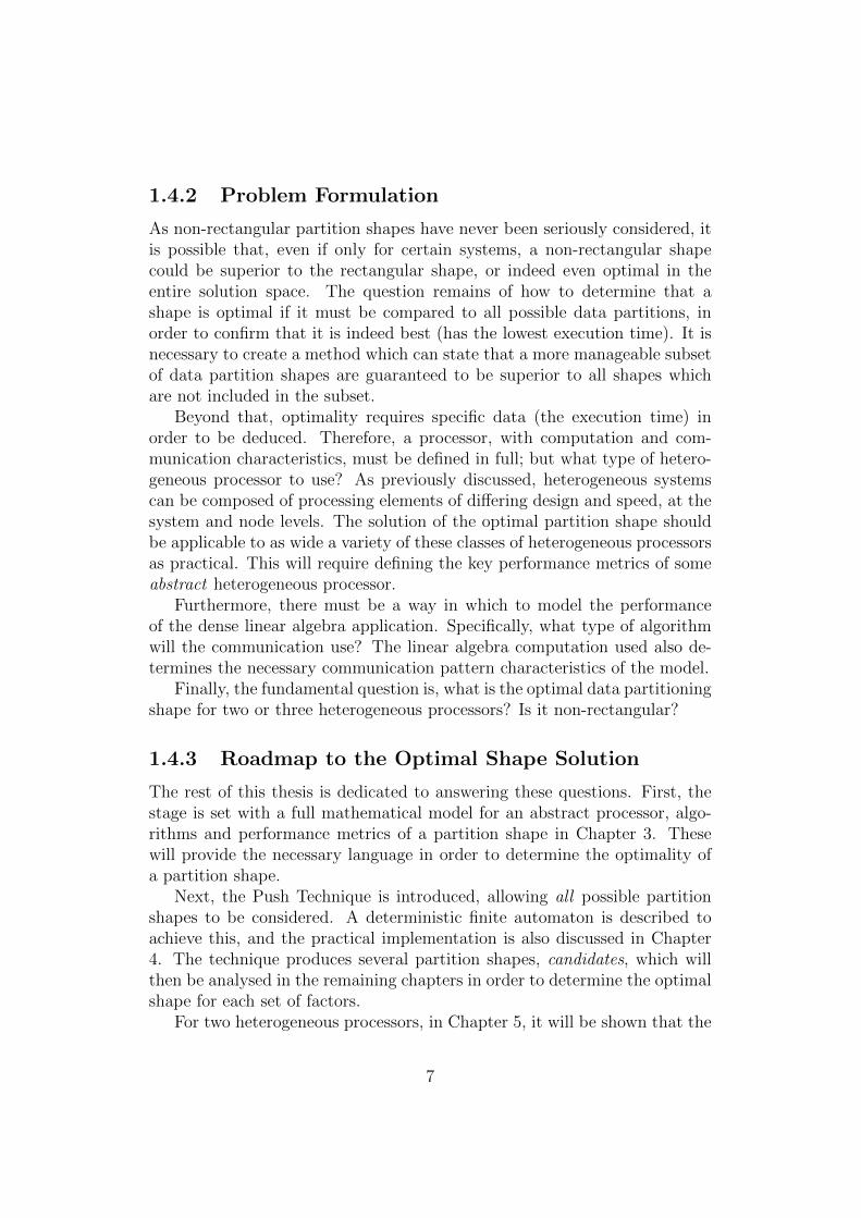
Matrix multiplication is a fundamental linear algebra operation. The generalconvention followed here is to name the square input matrices A and B,and the product matrix C. An element of matrix C is the product of thecorresponding row of matrix A and column of matrix B. Matrix A musthave N columns, and matrix B must have N rows. This calculation requiresN2 dot products, which each require N multiplications, thus, naively, matrixmultiplication is said to require N3 multiplications. Various algorithms havebeen shown to reduce this number, with the current minimum being N2.3727
[30].In the past, some of the simpler reductions, such as Strassen’s algorithm
9
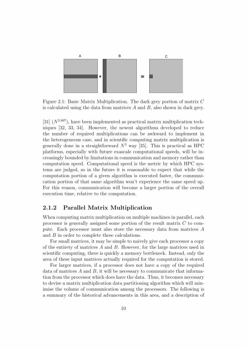
A B C
Figure 2.1: Basic Matrix Multiplication. The dark grey portion of matrix Cis calculated using the data from matrices A and B, also shown in dark grey.
[31] (N2.807), have been implemented as practical matrix multiplication tech-niques [32, 33, 34]. However, the newest algorithms developed to reducethe number of required multiplications can be awkward to implement inthe heterogeneous case, and in scientific computing matrix multiplication isgenerally done in a straightforward N3 way [35]. This is practical as HPCplatforms, especially with future exascale computational speeds, will be in-creasingly bounded by limitations in communication and memory rather thancomputation speed. Computational speed is the metric by which HPC sys-tems are judged, so in the future it is reasonable to expect that while thecomputation portion of a given algorithm is executed faster, the communi-cation portion of that same algorithm won’t experience the same speed up.For this reason, communication will become a larger portion of the overallexecution time, relative to the computation.
2.1.2 Parallel Matrix Multiplication
When computing matrix multiplication on multiple machines in parallel, eachprocessor is generally assigned some portion of the result matrix C to com-pute. Each processor must also store the necessary data from matrices Aand B in order to complete these calculations.
For small matrices, it may be simple to naively give each processor a copyof the entirety of matrices A and B. However, for the large matrices used inscientific computing, there is quickly a memory bottleneck. Instead, only thearea of these input matrices actually required for the computation is stored.
For larger matrices, if a processor does not have a copy of the requireddata of matrices A and B, it will be necessary to communicate that informa-tion from the processor which does have the data. Thus, it becomes necessaryto devise a matrix multiplication data partitioning algorithm which will min-imise the volume of communication among the processors. The following isa summary of the historical advancements in this area, and a description of
10
the current state of the art.
Cannon’s Algorithm and Fox’s Algorithm
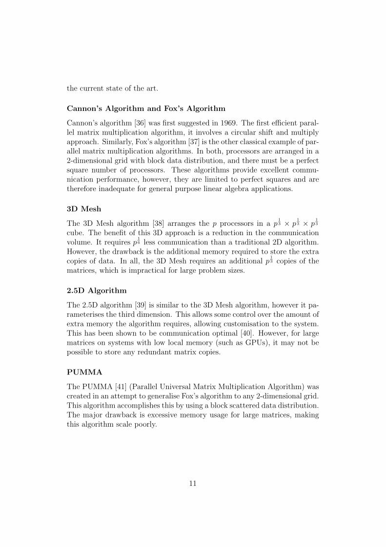
Cannon’s algorithm [36] was first suggested in 1969. The first efficient paral-lel matrix multiplication algorithm, it involves a circular shift and multiplyapproach. Similarly, Fox’s algorithm [37] is the other classical example of par-allel matrix multiplication algorithms. In both, processors are arranged in a2-dimensional grid with block data distribution, and there must be a perfectsquare number of processors. These algorithms provide excellent commu-nication performance, however, they are limited to perfect squares and aretherefore inadequate for general purpose linear algebra applications.
3D Mesh
The 3D Mesh algorithm [38] arranges the p processors in a p13 × p
13 × p
13
cube. The benefit of this 3D approach is a reduction in the communicationvolume. It requires p
16 less communication than a traditional 2D algorithm.
However, the drawback is the additional memory required to store the extracopies of data. In all, the 3D Mesh requires an additional p
13 copies of the
matrices, which is impractical for large problem sizes.
2.5D Algorithm
The 2.5D algorithm [39] is similar to the 3D Mesh algorithm, however it pa-rameterises the third dimension. This allows some control over the amount ofextra memory the algorithm requires, allowing customisation to the system.This has been shown to be communication optimal [40]. However, for largematrices on systems with low local memory (such as GPUs), it may not bepossible to store any redundant matrix copies.
PUMMA
The PUMMA [41] (Parallel Universal Matrix Multiplication Algorithm) wascreated in an attempt to generalise Fox’s algorithm to any 2-dimensional grid.This algorithm accomplishes this by using a block scattered data distribution.The major drawback is excessive memory usage for large matrices, makingthis algorithm scale poorly.
11
State of the Art: SUMMA
The SUMMA [29] (Scalable Universal Matrix Multiplication Algorithm) isan improvement of the PUMMA algorithm, looking to, as the name wouldsuggest, make the PUMMA algorithm scalable. The SUMMA algorithm,although nearly two decades old, is still considered to be a state of the artalgorithm. It is currently in use in popular linear algebra packages, such asScaLAPACK [25]. For this reason, it is discussed in more detail here thanthe other algorithms.
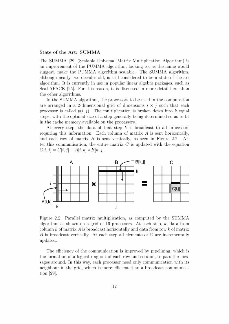
In the SUMMA algorithm, the processors to be used in the computationare arranged in a 2-dimensional grid of dimensions i × j such that eachprocessor is called p(i, j). The multiplication is broken down into k equalsteps, with the optimal size of a step generally being determined so as to fitin the cache memory available on the processors.
At every step, the data of that step k is broadcast to all processorsrequiring this information. Each column of matrix A is sent horizontally,and each row of matrix B is sent vertically, as seen in Figure 2.2. Af-ter this communication, the entire matrix C is updated with the equationC[i, j] = C[i, j] + A[i, k] ∗B[k, j].
i
k j
k
A B C
A[i,k]
C[i,j]
B[k,j]
Figure 2.2: Parallel matrix multiplication, as computed by the SUMMAalgorithm as shown on a grid of 16 processors. At each step, k, data fromcolumn k of matrix A is broadcast horizontally and data from row k of matrixB is broadcast vertically. At each step all elements of C are incrementallyupdated.
The efficiency of the communication is improved by pipelining, which isthe formation of a logical ring out of each row and column, to pass the mes-sages around. In this way, each processor need only communication with itsneighbour in the grid, which is more efficient than a broadcast communica-tion [29].
12
The overall cost of this algorithm is good for such a general solution. Itis computationally balanced, and achieves within log p of the communicationlower bound.
Recent Additions to SUMMA
Several algorithms have attempted to build on the SUMMA algorithmic de-sign. The SRUMMA [42] (Shared and Remote-memory based Universal Ma-trix Multiplication Algorithm) has a complexity comparable to Cannon’salgorithm, but uses shared memory and remote memory access instead ofmessage passing. This makes it appropriate for clusters and shared memorysystems.
The HSUMMA [19] (Hierarchical Scalable Universal Matrix Multiplica-tion Algorithm) is another recent extension of the SUMMA algorithm. Itadds a hierarchical, two dimensional decomposition to SUMMA in order toreduce the communication cost of the algorithm.
2.2 Rectangular Data Partitioning
This section includes a review of previous work in the area of data partition-ing for linear algebra applications. The problem of optimally partitioningheterogeneous processors in a general way is NP -complete [28, 43]. How-ever, a number of limited solutions have been created, and some commonsub-optimal rectangular partitioning schemes are presented here.
In all cases, the matrices are assumed to be identically partitioned acrossmatrices A,B, and C. As is found throughout the literature, especiallythose discussed below, a change in any partition shape will be reflected inthe partition shape for all matrices. For this reason, the partition shapeis displayed as a single matrix and it is understood to represent all threematrices.
2.2.1 One-Dimensional Partitioning
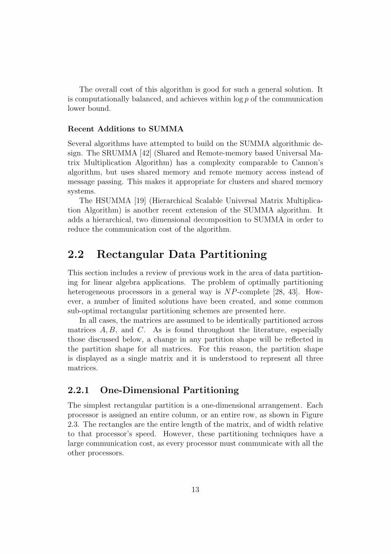
The simplest rectangular partition is a one-dimensional arrangement. Eachprocessor is assigned an entire column, or an entire row, as shown in Figure2.3. The rectangles are the entire length of the matrix, and of width relativeto that processor’s speed. However, these partitioning techniques have alarge communication cost, as every processor must communicate with all theother processors.
13
P0 P1 P2 P3
(a) 1D Columns
P0
P1
P2
P3
(b) 1D Rows
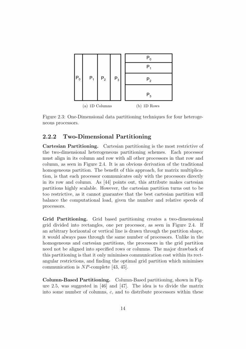
Figure 2.3: One-Dimensional data partitioning techniques for four heteroge-neous processors.
2.2.2 Two-Dimensional Partitioning
Cartesian Partitioning. Cartesian partitioning is the most restrictive ofthe two-dimensional heterogeneous partitioning schemes. Each processormust align in its column and row with all other processors in that row andcolumn, as seen in Figure 2.4. It is an obvious derivation of the traditionalhomogeneous partition. The benefit of this approach, for matrix multiplica-tion, is that each processor communicates only with the processors directlyin its row and column. As [44] points out, this attribute makes cartesianpartitions highly scalable. However, the cartesian partition turns out to betoo restrictive, as it cannot guarantee that the best cartesian partition willbalance the computational load, given the number and relative speeds ofprocessors.
Grid Partitioning. Grid based partitioning creates a two-dimensionalgrid divided into rectangles, one per processor, as seen in Figure 2.4. Ifan arbitrary horizontal or vertical line is drawn through the partition shape,it would always pass through the same number of processors. Unlike in thehomogeneous and cartesian partitions, the processors in the grid partitionneed not be aligned into specified rows or columns. The major drawback ofthis partitioning is that it only minimises communication cost within its rect-angular restrictions, and finding the optimal grid partition which minimisescommunication is NP -complete [43, 45].
Column-Based Partitioning. Column-Based partitioning, shown in Fig-ure 2.5, was suggested in [46] and [47]. The idea is to divide the matrixinto some number of columns, c, and to distribute processors within these
14
P11 P12 P13 P14
P21 P22 P23 P24
P31 P32 P33 P34
P41 P42 P43 P44
(a) Homogeneous
P11 P12 P13 P14
P21 P22 P23 P24
P31 P32 P33 P34
P41 P42 P43 P44
(b) Cartesian
P11 P12 P13 P14
P21 P22 P23 P24
P31 P32 P33 P34
P41 P42 P43 P44
(c) Grid
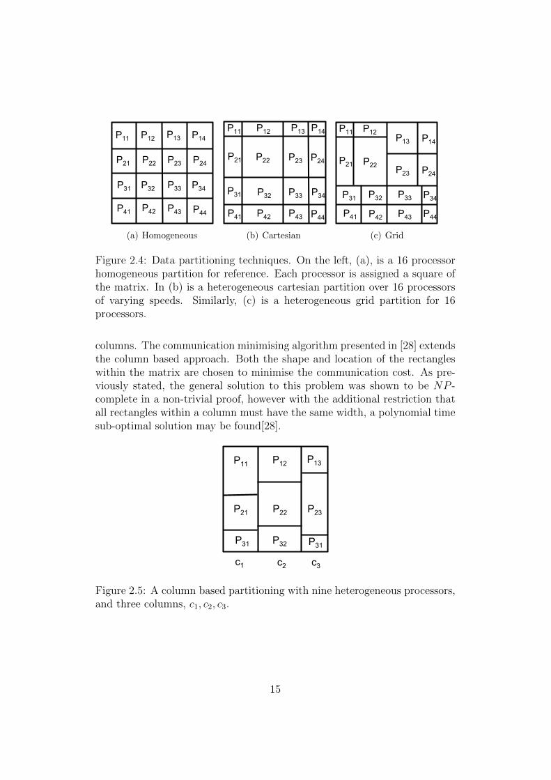
Figure 2.4: Data partitioning techniques. On the left, (a), is a 16 processorhomogeneous partition for reference. Each processor is assigned a square ofthe matrix. In (b) is a heterogeneous cartesian partition over 16 processorsof varying speeds. Similarly, (c) is a heterogeneous grid partition for 16processors.
columns. The communication minimising algorithm presented in [28] extendsthe column based approach. Both the shape and location of the rectangleswithin the matrix are chosen to minimise the communication cost. As pre-viously stated, the general solution to this problem was shown to be NP -complete in a non-trivial proof, however with the additional restriction thatall rectangles within a column must have the same width, a polynomial timesub-optimal solution may be found[28].
P11 P12 P13
P21 P22 P23
P31 P32 P31
c1 c2 c3
Figure 2.5: A column based partitioning with nine heterogeneous processors,and three columns, c1, c2, c3.
15
2.2.3 Performance Model Based Partitioning
The previously discussed partitioning algorithms all assumed a constant per-formance model for the processors. Each processor is assigned a constantpositive value to represent its speed in proportion to the rest of the proces-sors. The benefit of this technique is its simplicity, as well as it’s accuracyfor small to medium, or constant, sized problem domains. However, for largeor fluctuating problem sizes, it is possible that the performance will changeleading to inaccuracy in the model, which can cause a degradation in theperformance of the overall application.
Functional Performance Modelling. Functional performance modelling[48, 49, 50] takes into consideration the problem size when estimating thespeed of a given processor. This allows for accurate modelling of processorperformance if the processor throughput degrades with problem size. Mostoften, this occurs when some physical limit of the processor is met, such asthe filling of cache memory, and a sudden and marked deterioration in perfor-mance occurs. With this clear physical limitation in mind, these functionalperformance models have been used to find data partitions for linear algebraapplications such as parallel matrix multiplication [51].
2.3 Non-Rectangular Data Partitioning
This section provides a survey of previous work that examined non-rectangularpartitioning of matrices for matrix multiplication. These results focus oncomparing two shapes, rather than considering their optimality. They alsoconsider only communication, not execution time, and shapes are not com-pared for a wide variety of performance model algorithms.
2.3.1 Two Processors
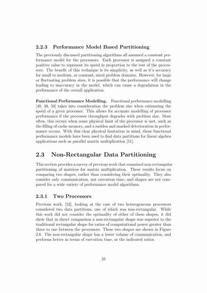
Previous work, [52], looking at the case of two heterogeneous processorsconsidered two data partitions, one of which was non-rectangular. Whilethis work did not consider the optimality of either of these shapes, it didshow that in direct comparison a non-rectangular shape was superior to thetraditional rectangular shape for ratios of computational power greater thanthree to one between the processors. These two shapes are shown in Figure2.6. The non-rectangular shape has a lower volume of communication, andperforms better in terms of execution time, at the indicated ratios.
16
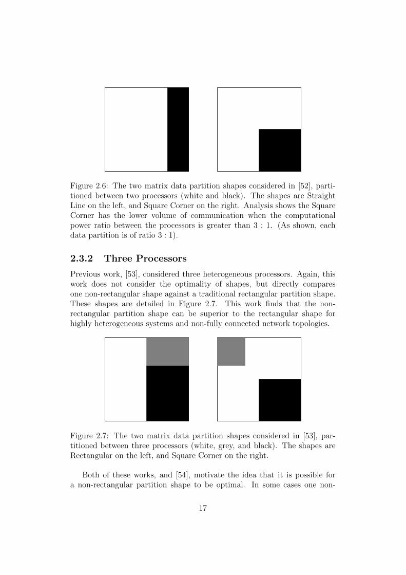
Figure 2.6: The two matrix data partition shapes considered in [52], parti-tioned between two processors (white and black). The shapes are StraightLine on the left, and Square Corner on the right. Analysis shows the SquareCorner has the lower volume of communication when the computationalpower ratio between the processors is greater than 3 : 1. (As shown, eachdata partition is of ratio 3 : 1).
2.3.2 Three Processors
Previous work, [53], considered three heterogeneous processors. Again, thiswork does not consider the optimality of shapes, but directly comparesone non-rectangular shape against a traditional rectangular partition shape.These shapes are detailed in Figure 2.7. This work finds that the non-rectangular partition shape can be superior to the rectangular shape forhighly heterogeneous systems and non-fully connected network topologies.
Figure 2.7: The two matrix data partition shapes considered in [53], par-titioned between three processors (white, grey, and black). The shapes areRectangular on the left, and Square Corner on the right.
Both of these works, and [54], motivate the idea that it is possible fora non-rectangular partition shape to be optimal. In some cases one non-
17
rectangular shape, the Square Corner, is superior to specific common rect-angular shapes. However, these previous works fail to address the concept ofoptimality or matrix computations other than matrix multiplication.
2.4 Abstract Processors
The notion of an abstract processor has previously been used to represent avariety of different real world heterogeneous systems.
In [55], the authors used abstract processor models to encapsulate multi-core processors. This approach was used to balance the computational loadfor matrix multiplication on multicore nodes of a heterogeneous multicorecluster.
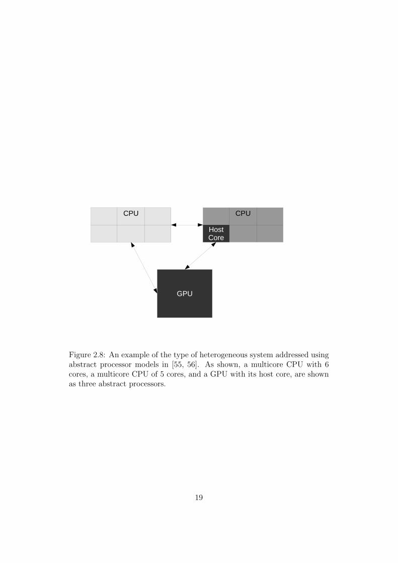
In [56], the authors extend this abstract processor model approach to beapplicable to both heterogeneous multicore and hybrid multicore CPU/GPUsystems, an example of which can be seen in Figure 2.8. Using this approach,they were able to accurately model the performance of different heteroge-neous configurations for scientific data parallel applications. These variousheterogeneous components were often described as systems of two or threeheterogeneous abstract processors. However, these works only considered tra-ditional, rectangular data partitions for these systems. The types of novel,non-rectangular data partition shapes presented in this thesis have neverbeen considered using this type of abstract processor model.
18
CPU CPU
Host Core
GPU
Figure 2.8: An example of the type of heterogeneous system addressed usingabstract processor models in [55, 56]. As shown, a multicore CPU with 6cores, a multicore CPU of 5 cores, and a GPU with its host core, are shownas three abstract processors.
19
Chapter 3
Modelling Matrix Computationon Abstract Processors
In this chapter, the complete performance model for the abstract heteroge-neous processor is presented. An abstract processor is any unit of processingpower which may receive, store, and compute data, and most importantly, isindependent. An independent processing unit is not affected by the compu-tational load placed on any other processing unit. For example, an indepen-dent processor is not affected by resource contention, as cores on the samedie would be. Examples of an independent processing unit include single andmulticore CPUs, a GPU and its host core, or an entire cluster.
The notion of an abstract processor, which focuses primarily on com-munication volume and computation volume, has been shown to accuratelypredict the experimental performance of a variety of processors and evenentire clusters for matrix computations [52, 53, 54, 57, 58]. Below, the com-munication, computation, and memory modelling of an abstract processor isdiscussed further in the context of matrix computations.
Data Partition Metrics
In order to effectively model the matrix computations, several assumptionsare made and partition metrics are devised.
• The matrices are square and of size N ×N elements
• The matrices are identically partitioned among p processors
• The number of elements assigned to each processor is factorable, i.e.may be made into a rectangle
20
Formally, a partition is an arrangement of elements amongst processorssuch that,
φ(i, j) =
0 Element (i, j) assigned to 1st Processor
1 Element (i, j) assigned to 2nd Processor
...
p− 1 Element (i, j) assigned to pth Processor
(3.1)
To determine whether a given row, i, contains elements that are assignedto a given processor, x,
r(φ, x, i) =
{0 if (i, ·) of φ is not assigned to Processor x
1 if some (i, ·) of φ is assigned to Processor x(3.2)
To determine whether a given column, j, contains elements that are as-signed to a given processor, x,
c(φ, x, j) =
{0 if (·, j) of φ is not assigned to Processor x
1 if some (·, j) of φ is assigned to Processor x(3.3)
Processor Naming Convention
The equations provided below are written in such a way to be applicable toany number of processors p, and correspondingly the xth processor is calledpx. However, for the small numbers of abstract processors studied in detail,it may be useful to call the processors by different letters, for clarity.
For two processors, the more powerful processor is known as Processor P ,and the less powerful as Processor S. The ratio between the computationalpower of these two processors is called r, and is normalised to be r : 1.
For three processors, the processors are called, in descending order ofcomputational power, Processor P , Processor R, and Processor S. The ratiobetween the computational power of these processors is Pr : Rr : Sr, and isnormalised to Pr : Rr : 1.
3.1 Communication Modelling
The communication of matrix multiplication may be modelled in a varietyof ways, depending on the level of specificity required. First is the questionof topology. Does a link exist between all processors? Then consider, are all
21
links between processors symmetrical? Are there significant startup costs insending an individual message?
When considering only small numbers of abstract processors, the possibletopologies are limited. For two processors, for instance, the only option isfully connected, or no communication would be possible. When consideringthree processors, the options are fully connected or a star topology, so theseare discussed in further detail below. Additionally, the focus is placed onsymmetric communications, and latency will be ignored due to its lessersignificance in the communication and computation volume in most of thealgorithms studied (specifically those which use bulk communication).
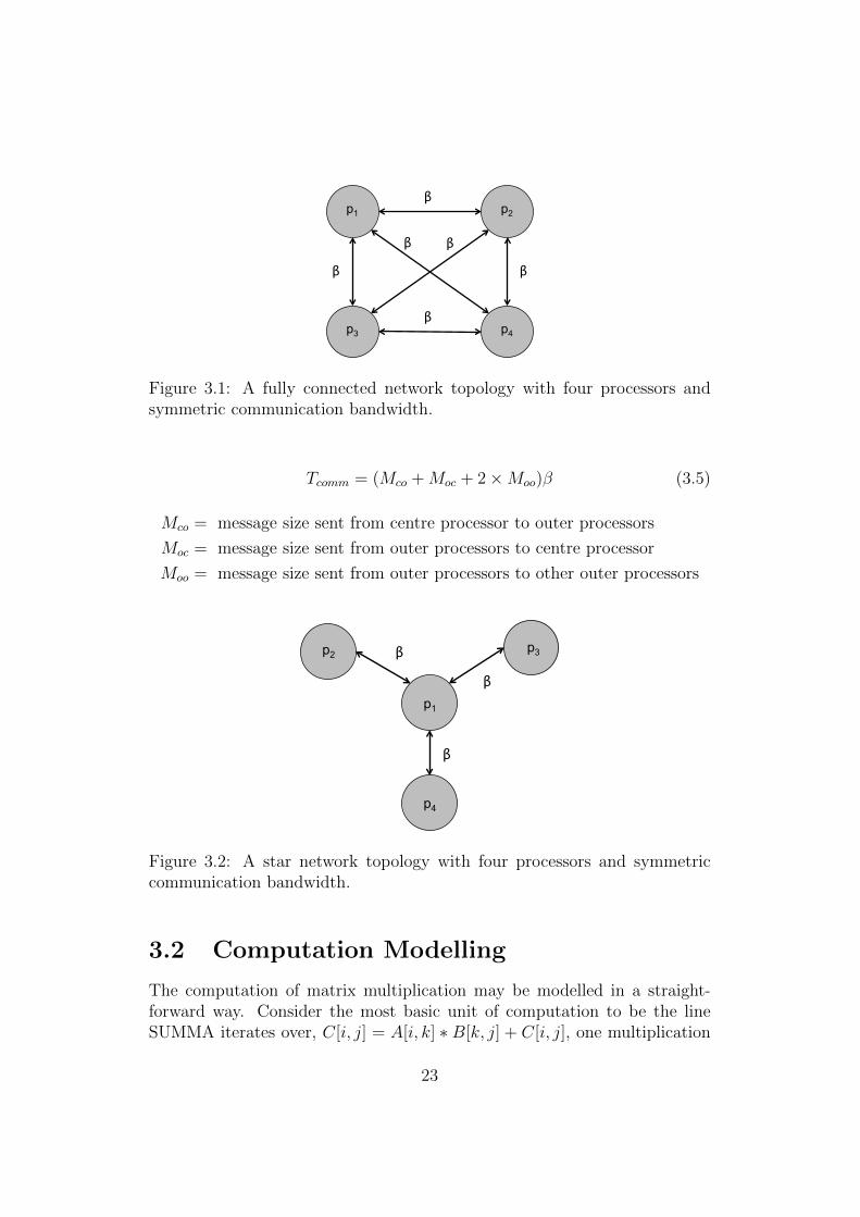
3.1.1 Fully Connected Network Topology
In the fully connected topology, each processor has a direct communicationlink to all p−1 other processors, as seen in Figure 3.1. The simplest model ofsymmetric communication is the Hockney Model [59]. This states the timeof communication is a factor of latency, bandwidth, and message size, and isgiven by,
Tcomm = α + βM (3.4)
α = 0 = the latency, overhead of sending one message in seconds
(which is insignificant compared to βM in this model, so set to zero)
β = the inverse of bandwidth, transfer time (in seconds) per element
(which for simplicity will be referred to as bandwidth throughout this thesis)
M = the message size, the number of elements to be sent
3.1.2 Star Network Topology
The star topology puts a single processor at the centre, with all other pro-cessors communicating through it, as seen in Figure 3.2. For most of thepartition shapes that will be found using the Push Technique, the data thatan outer processor sends to the centre processor is not the same data (i.e.it comes from a different location or matrix) as it sends to some other outerprocessor. For this reason, the outer-to-outer term in the communicationtime equation is doubled. This may be possible to improve upon, depend-ing on the partition shape, however this equation represents the worst casescenario.
22
p1 p2
p3 p4
β
β β
β β
β
Figure 3.1: A fully connected network topology with four processors andsymmetric communication bandwidth.
Tcomm = (Mco +Moc + 2×Moo)β (3.5)
Mco = message size sent from centre processor to outer processors
Moc = message size sent from outer processors to centre processor
Moo = message size sent from outer processors to other outer processors
p1
p3
p4
β
β
β p2
Figure 3.2: A star network topology with four processors and symmetriccommunication bandwidth.
3.2 Computation Modelling
The computation of matrix multiplication may be modelled in a straight-forward way. Consider the most basic unit of computation to be the lineSUMMA iterates over, C[i, j] = A[i, k] ∗ B[k, j] + C[i, j], one multiplication
23
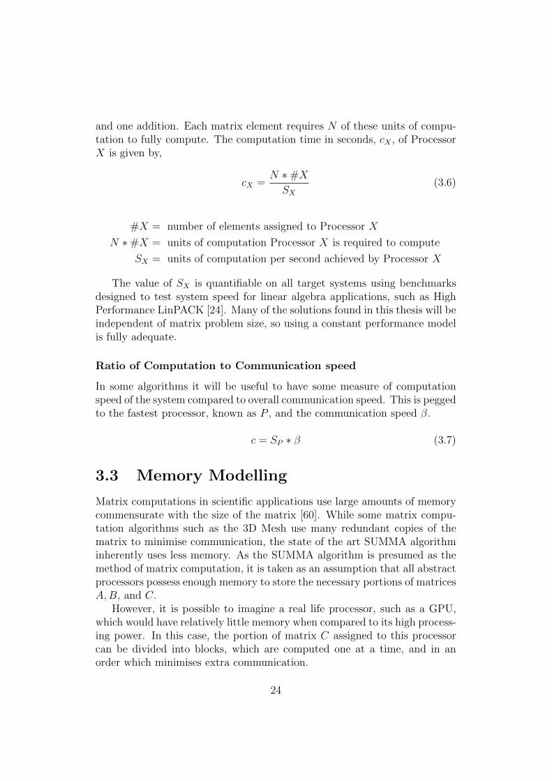
and one addition. Each matrix element requires N of these units of compu-tation to fully compute. The computation time in seconds, cX , of ProcessorX is given by,
cX =N ∗#X
SX(3.6)
#X = number of elements assigned to Processor X
N ∗#X = units of computation Processor X is required to compute
SX = units of computation per second achieved by Processor X
The value of SX is quantifiable on all target systems using benchmarksdesigned to test system speed for linear algebra applications, such as HighPerformance LinPACK [24]. Many of the solutions found in this thesis will beindependent of matrix problem size, so using a constant performance modelis fully adequate.
Ratio of Computation to Communication speed
In some algorithms it will be useful to have some measure of computationspeed of the system compared to overall communication speed. This is peggedto the fastest processor, known as P , and the communication speed β.
c = SP ∗ β (3.7)
3.3 Memory Modelling
Matrix computations in scientific applications use large amounts of memorycommensurate with the size of the matrix [60]. While some matrix compu-tation algorithms such as the 3D Mesh use many redundant copies of thematrix to minimise communication, the state of the art SUMMA algorithminherently uses less memory. As the SUMMA algorithm is presumed as themethod of matrix computation, it is taken as an assumption that all abstractprocessors possess enough memory to store the necessary portions of matricesA,B, and C.
However, it is possible to imagine a real life processor, such as a GPU,which would have relatively little memory when compared to its high process-ing power. In this case, the portion of matrix C assigned to this processorcan be divided into blocks, which are computed one at a time, and in anorder which minimises extra communication.
24
3.4 Algorithm Description
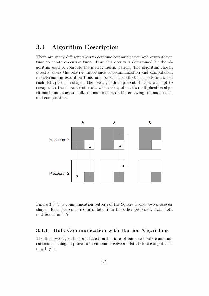
There are many different ways to combine communication and computationtime to create execution time. How this occurs is determined by the al-gorithm used to compute the matrix multiplication. The algorithm chosendirectly alters the relative importance of communication and computationin determining execution time, and so will also effect the performance ofeach data partition shape. The five algorithms presented below attempt toencapsulate the characteristics of a wide variety of matrix multiplication algo-rithms in use, such as bulk communication, and interleaving communicationand computation.
Figure 3.3: The communication pattern of the Square Corner two processorshape. Each processor requires data from the other processor, from bothmatrices A and B.
3.4.1 Bulk Communication with Barrier Algorithms
The first two algorithms are based on the idea of barriered bulk communi-cations, meaning all processors send and receive all data before computationmay begin.
25
(Execution Begins) P S
(Execution Complete)
P sends S sends
PCB Algorithm
(Barrier)
(Barrier)
P S
(Execution Complete)
P sends
S sends
SCB Algorithm
P computes S computes
P computes S computes
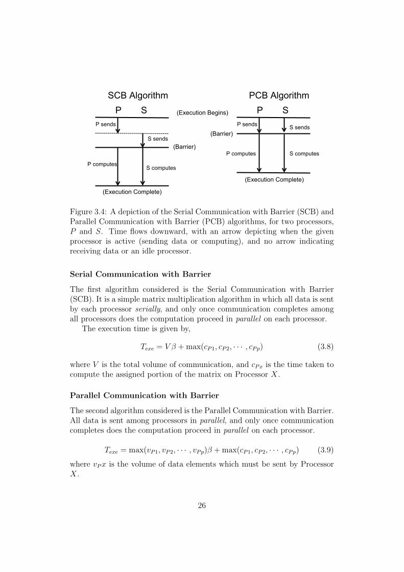
Figure 3.4: A depiction of the Serial Communication with Barrier (SCB) andParallel Communication with Barrier (PCB) algorithms, for two processors,P and S. Time flows downward, with an arrow depicting when the givenprocessor is active (sending data or computing), and no arrow indicatingreceiving data or an idle processor.
Serial Communication with Barrier
The first algorithm considered is the Serial Communication with Barrier(SCB). It is a simple matrix multiplication algorithm in which all data is sentby each processor serially, and only once communication completes amongall processors does the computation proceed in parallel on each processor.
The execution time is given by,
Texe = V β + max(cP1, cP2, · · · , cPp) (3.8)
where V is the total volume of communication, and cPx is the time taken tocompute the assigned portion of the matrix on Processor X.
Parallel Communication with Barrier
The second algorithm considered is the Parallel Communication with Barrier.All data is sent among processors in parallel, and only once communicationcompletes does the computation proceed in parallel on each processor.
Texe = max(vP1, vP2, · · · , vPp)β + max(cP1, cP2, · · · , cPp) (3.9)
where vPx is the volume of data elements which must be sent by ProcessorX.
26
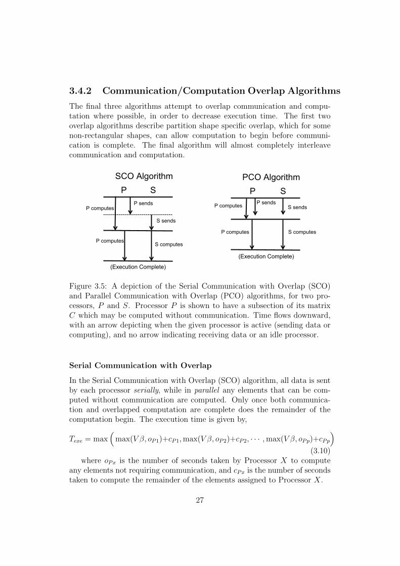
3.4.2 Communication/Computation Overlap Algorithms
The final three algorithms attempt to overlap communication and compu-tation where possible, in order to decrease execution time. The first twooverlap algorithms describe partition shape specific overlap, which for somenon-rectangular shapes, can allow computation to begin before communi-cation is complete. The final algorithm will almost completely interleavecommunication and computation.
P S
(Execution Complete)
P sends
S sends
SCO Algorithm
P computes S computes
P computes
P S
(Execution Complete)
P sends S sends
PCO Algorithm
P computes S computes
P computes
Figure 3.5: A depiction of the Serial Communication with Overlap (SCO)and Parallel Communication with Overlap (PCO) algorithms, for two pro-cessors, P and S. Processor P is shown to have a subsection of its matrixC which may be computed without communication. Time flows downward,with an arrow depicting when the given processor is active (sending data orcomputing), and no arrow indicating receiving data or an idle processor.
Serial Communication with Overlap
In the Serial Communication with Overlap (SCO) algorithm, all data is sentby each processor serially, while in parallel any elements that can be com-puted without communication are computed. Only once both communica-tion and overlapped computation are complete does the remainder of thecomputation begin. The execution time is given by,
Texe = max(
max(V β, oP1)+cP1,max(V β, oP2)+cP2, · · · ,max(V β, oPp)+cPp
)(3.10)
where oPx is the number of seconds taken by Processor X to computeany elements not requiring communication, and cPx is the number of secondstaken to compute the remainder of the elements assigned to Processor X.
27
Parallel Communication with Overlap
The Parallel Communication with Overlap (PCO) algorithm, completes allcommunication in parallel, while simultaneously computing any sections ofmatrix C which do not require interprocessor communication. Once thesehave finished, the remainder of the computation is carried out. The executiontime is given by,
Texe = max(
max(Tcomm, oP1) + cP1,max(Tcomm, oP2) + cP2, · · · ,
max(Tcomm, oPp) + cPp
)(3.11)
where Tcomm is the same as the PCB algorithm, oPx is the number ofseconds taken by Processor X to compute any elements not requiring com-munication, and cPx is the number of seconds taken to compute the remainderof the elements assigned to Processor X.
Parallel Interleaving Overlap
The Parallel Interleaving Overlap (PIO) algorithm, unlike the previous al-gorithms described, does not use bulk communication. At each step data issent, a row and a column (or k rows and columns) at a time, by the relevantprocessor(s) to all processor(s) requiring those elements, while, in parallel, allprocessors compute using the data sent in the previous step. The executiontime for this algorithm is given by,
Texe = Send k +
(N − 1) max(Vkβ,max
(kP1, kP2, · · · , kPp
))+ Compute (k + 1) (3.12)
where Vk is the number of elements sent at step k, and kX is the numberof seconds to compute step k on Processor X.
28
Chapter 4
The Push Technique
The central contribution of this thesis is the introduction of the Push Tech-nique. This novel method alters a matrix data partition, reassigning elementsamong processors, to lower the total volume of communication of the parti-tion shape. The goal of using this technique is to prove that some randomarrangement of elements is not the optimal shape. Instead, it allows theconsideration of a few discrete partition shapes which are superior to allother data partitions (by virtue of the fact that no Push operation can beperformed on them).
The Push Technique operates on an individual processor (although ona given Push any and all processors may be reassigned elements) and anindividual row or column. That row or column, k, is determined by the di-rection of the Push (Up, Down, Back, or Over) and the enclosing rectangleof the processor being Pushed. An enclosing rectangle is an imaginary rect-angle drawn around the elements of a given processor, which is strictly largeenough to encompass all such elements, as seen in Figure 4.1. The edgesof some Processor X’s enclosing rectangle are known in clockwise order asxtop, xright, xbottom, xleft.
4.1 General Form
When applying the Push Technique to a data partition shape containing anarbitrary number of processors,
• Choose one processor, X, to be Pushed (must not be the most powerfulprocessor)
• Choose the direction of Push, i.e. Up (↑), Down (↓), Back (←), Over(→)
29
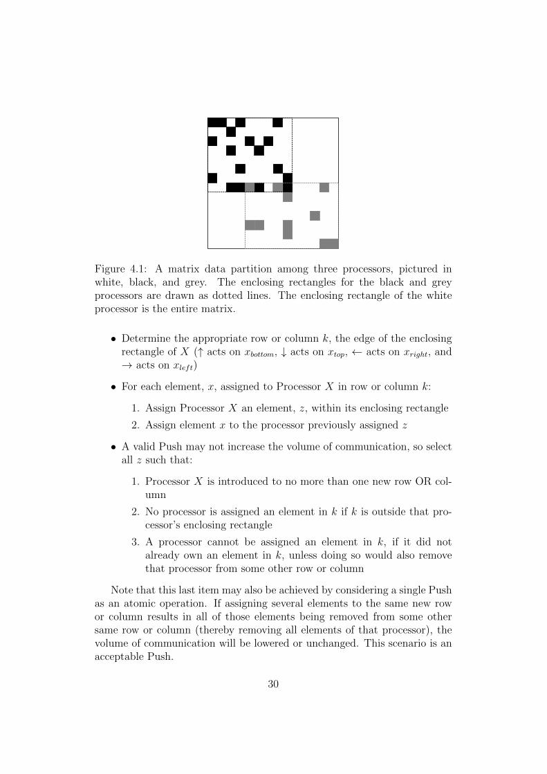
Figure 4.1: A matrix data partition among three processors, pictured inwhite, black, and grey. The enclosing rectangles for the black and greyprocessors are drawn as dotted lines. The enclosing rectangle of the whiteprocessor is the entire matrix.
• Determine the appropriate row or column k, the edge of the enclosingrectangle of X (↑ acts on xbottom, ↓ acts on xtop, ← acts on xright, and→ acts on xleft)
• For each element, x, assigned to Processor X in row or column k:
1. Assign Processor X an element, z, within its enclosing rectangle
2. Assign element x to the processor previously assigned z
• A valid Push may not increase the volume of communication, so selectall z such that:
1. Processor X is introduced to no more than one new row OR col-umn
2. No processor is assigned an element in k if k is outside that pro-cessor’s enclosing rectangle
3. A processor cannot be assigned an element in k, if it did notalready own an element in k, unless doing so would also removethat processor from some other row or column
Note that this last item may also be achieved by considering a single Pushas an atomic operation. If assigning several elements to the same new rowor column results in all of those elements being removed from some othersame row or column (thereby removing all elements of that processor), thevolume of communication will be lowered or unchanged. This scenario is anacceptable Push.
30
4.2 Using the Push Technique to solve the
Optimal Data Partition Shape Problem
The Push Technique may be applied iteratively to a data partition shape,incrementally improving it until a shape is reached on which no valid Pushoperations may be performed. Any such data partition, with no possible Pushoperations, is a candidate to be optimal and must be considered further.
In general, the Push Technique will be applied to some random startingpartition. Push operations are performed until some local minima is found,where no further Push operations are possible. Those final states are thecandidates considered throughout this thesis.
Consider a Deterministic Finite Automaton. This DFA is a 5-tuple(Q,Σ, δ, q0, F ) where
1. Q is the finite set of states, the possible data partitioning shapes
2. Σ is the finite set of the alphabet, the processors and the directionsthey can be Pushed
3. δ is Q× Σ→ Q the transition function, the Push operation
4. q0, the start state, chosen at random
5. F is F ⊆ Q, the accept states, candidate partitions to be the optimum
The finite set of states, Q, is every possible permutation of the elements,assigned to each processor, within the N ×N matrix. Therefore the numberof states in the DFA is dependent on the size of the matrix, the number ofprocessors and the relative processing speeds of those processors. The sizeof Q is given by
N2!
(#P1!)× (#P2!)× · · · × (#Pp!)(4.1)
where,#Px is the number of elements assigned to Processor X
The finite set, Σ, called the alphabet, is the information processed by thetransition function in order to move between states. Legal input symbolsare the active processor being Pushed, Processor X, and the direction theelements of Processor X are to be moved, i.e. Up, Down, Over or Back.
The transition function, δ, is the Push operation. This function processesthe input language Σ and moves the DFA from one state to the next, and
31
therefore the matrix from one partition shape to the next. The implementa-tion of the transition function is discussed further in the next section. If theelements of the specified processor cannot be moved in the specified directionthen the state is not changed, i.e. the transition arrow loops back onto thecurrent state for that input.
The start state of the DFA, q0, is chosen randomly.Finally, the accept states F are those fixed points in which no Processor
X may be Pushed in any direction. These states, and their correspondingpartition shapes, must be studied further.
4.3 Application to Matrix Multiplication
The Push Technique, as described above for any number of processors, willalso be detailed for specific applications of two and three processors, withfurther insight into how the Push can apply to four and more processors.This entire chapter is dedicated to the Push Technique as it applies to matrixmultiplication, so it is worth noting now which parts are constant, and whichchange when applying to other matrix computations.
The Push Technique, so far as it is a methodology for incrementally al-tering a matrix partition for the better, is applicable to nearly any matrixcomputation. The difference, and what makes the remainder of this chapterspecific to matrix multiply, is the performance model (volume of communi-cation) the Push is operating under. The rules of the Push could, therefore,be altered to prejudice for some other metric(s) and create different matrixpartitions for different computational needs.
Matrix multiplication is straightforward with easily parallelised compu-tation and simple communication patterns, and as such is the best startingpoint for applying the Push Technique. However, any matrix computationwhich can be decomposed into some quantifiable incremental changes, canbenefit from the Push Technique.
4.4 Push Technique on a Two Processor Sys-
tem
The two processor case is the simplest to which the Push Technique may beapplied. This provides an excellent base case for describing the basics of thePush, before moving on to the more complex issues of three, four, and moreprocessors.
32
This section first covers the algorithm used to carry out a single Pushoperation. The following section will show that continuous use of the Push,until no valid Push operations remain untaken, will result in a lower vol-ume of communication, and thereby lower execution time, for all five matrixmultiplication algorithms considered. Finally, the outcomes of these Pushoperations, the optimal candidates, are described.
4.4.1 Algorithmic Description
The algorithm used to accomplish the Push operation is given in more detailhere. Each direction is deterministic, and moves element in a typewriter-likefashion, i.e. left to right, and top to bottom.
Elements assigned to S in row k, (set to stop, in the example below), arereassigned to Processor P . Suitable elements are assigned to Processor S,from Processor P , from the rows below k and within the enclosing rectangleof Processor S. Assume S is the second processor, so φ(i, j) = 1 if element(i, j) is assigned to Processor S.
Push Down
Formally, Push ↓ (φ, k) = φ1 where,
Initialise φ1 ← φ(g, h) = (k + 1, sleft)for j = sleft → sright do{If element belongs Processor S, reassign it.}if φ(k, j) == 1 thenφ1(k, j) = 0;(g, h) = find(g, h); {Function defined below (finds new location).}φ1(g, h) = 1; {Assign new location to active processor.}
end ifj ← j + 1;
end for
find(g, h):
for g → sbottom dofor h→ sright do{If potential location belongs to other processor, hasn’t been reas-signed already, and is in a column already containing X.}if φ(g, h) == 0 && φ1(g, h) == 0 && c(φ, S, h) == 1 then
return (g, h);end if
33
end forg ← g + 1;h← sleft;
end forreturn φ1 = φ {Could not find location, Push not possible in this direc-tion.}It is important to note that if no suitable φ(g, h) can be found for each
element in the row being cleaned that requires rearrangement, then φ isconsidered fully condensed from the top and all further ↓ (φ, k) = φ.
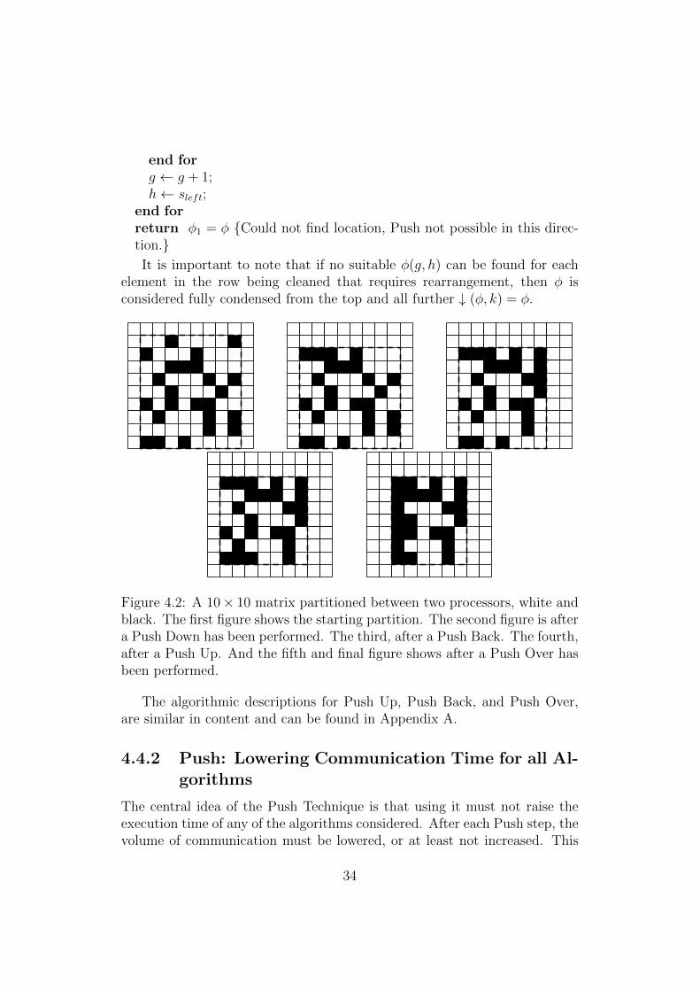
Figure 4.2: A 10× 10 matrix partitioned between two processors, white andblack. The first figure shows the starting partition. The second figure is aftera Push Down has been performed. The third, after a Push Back. The fourth,after a Push Up. And the fifth and final figure shows after a Push Over hasbeen performed.
The algorithmic descriptions for Push Up, Push Back, and Push Over,are similar in content and can be found in Appendix A.
4.4.2 Push: Lowering Communication Time for all Al-gorithms
The central idea of the Push Technique is that using it must not raise theexecution time of any of the algorithms considered. After each Push step, thevolume of communication must be lowered, or at least not increased. This
34
section demonstrates that the Push Technique will lower, or leave unchanged,the communication for each algorithm.
A data partition between two processors has a special metric,
‖ φ ‖x = # of rows containing elements of only one processor in φ
‖ φ ‖y = # of columns containing elements of only one processor in φ
Serial Communication.
Theorem 4.4.1 (Push). The Push Technique output partition, φ1, will havelower, or at worst equal, communication time as the input partition, φ.
Proof. First, observe several axioms related to the Push Technique.
Axiom 1. Push ↓ and Push ↑, create a row, k, with no elements belongingto the Pushed Processor X, and may introduce Processor X to at most onerow in φ1 in which there were no elements of Processor X in φ. No morethan one row can have elements of X introduced, as a row that was had noelements of X in φ will have enough suitable slots for all elements movedfrom the single row, k.
Axiom 2. Push ↓ and Push ↑ are defined to not add elements of Processor Xto a column in φ1 if there is no elements of X in that column of φ. However,these Push directions may create additional column(s) without X, if the rowk being Pushed contains elements that are the only elements of X in theircolumn, and there are sufficient suitable slots in other columns.
Axiom 3. Push → and Push ← create a column, k, with no elements be-longing to Processor X, and may create at most one column with X in φ1
that did not contain X in φ.
Axiom 4. Push→ and Push← will never add elements of X to a row in φ1
that did not contain elements of X in φ, but may create additional row(s)without X.
From (3.8) we observe as (‖ φ ‖x + ‖ φ ‖y) increases, Tcomm decreases.
35
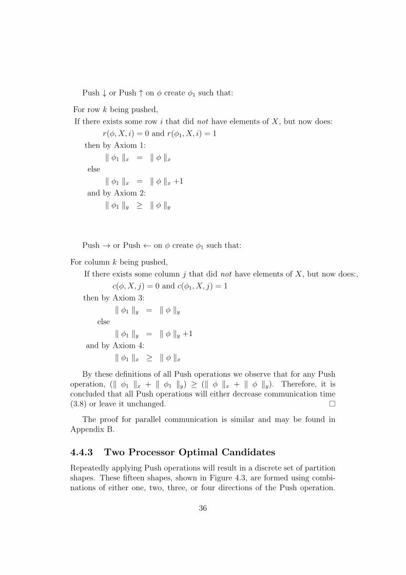
Push ↓ or Push ↑ on φ create φ1 such that:
For row k being pushed,
If there exists some row i that did not have elements of X, but now does:
r(φ,X, i) = 0 and r(φ1, X, i) = 1
then by Axiom 1:
‖ φ1 ‖x = ‖ φ ‖xelse
‖ φ1 ‖x = ‖ φ ‖x +1
and by Axiom 2:
‖ φ1 ‖y ≥ ‖ φ ‖y
Push → or Push ← on φ create φ1 such that:
For column k being pushed,
If there exists some column j that did not have elements of X, but now does:,
c(φ,X, j) = 0 and c(φ1, X, j) = 1
then by Axiom 3:
‖ φ1 ‖y = ‖ φ ‖yelse
‖ φ1 ‖y = ‖ φ ‖y +1
and by Axiom 4:
‖ φ1 ‖x ≥ ‖ φ ‖x
By these definitions of all Push operations we observe that for any Pushoperation, (‖ φ1 ‖x + ‖ φ1 ‖y) ≥ (‖ φ ‖x + ‖ φ ‖y). Therefore, it isconcluded that all Push operations will either decrease communication time(3.8) or leave it unchanged.
The proof for parallel communication is similar and may be found inAppendix B.
4.4.3 Two Processor Optimal Candidates
Repeatedly applying Push operations will result in a discrete set of partitionshapes. These fifteen shapes, shown in Figure 4.3, are formed using combi-nations of either one, two, three, or four directions of the Push operation.
36
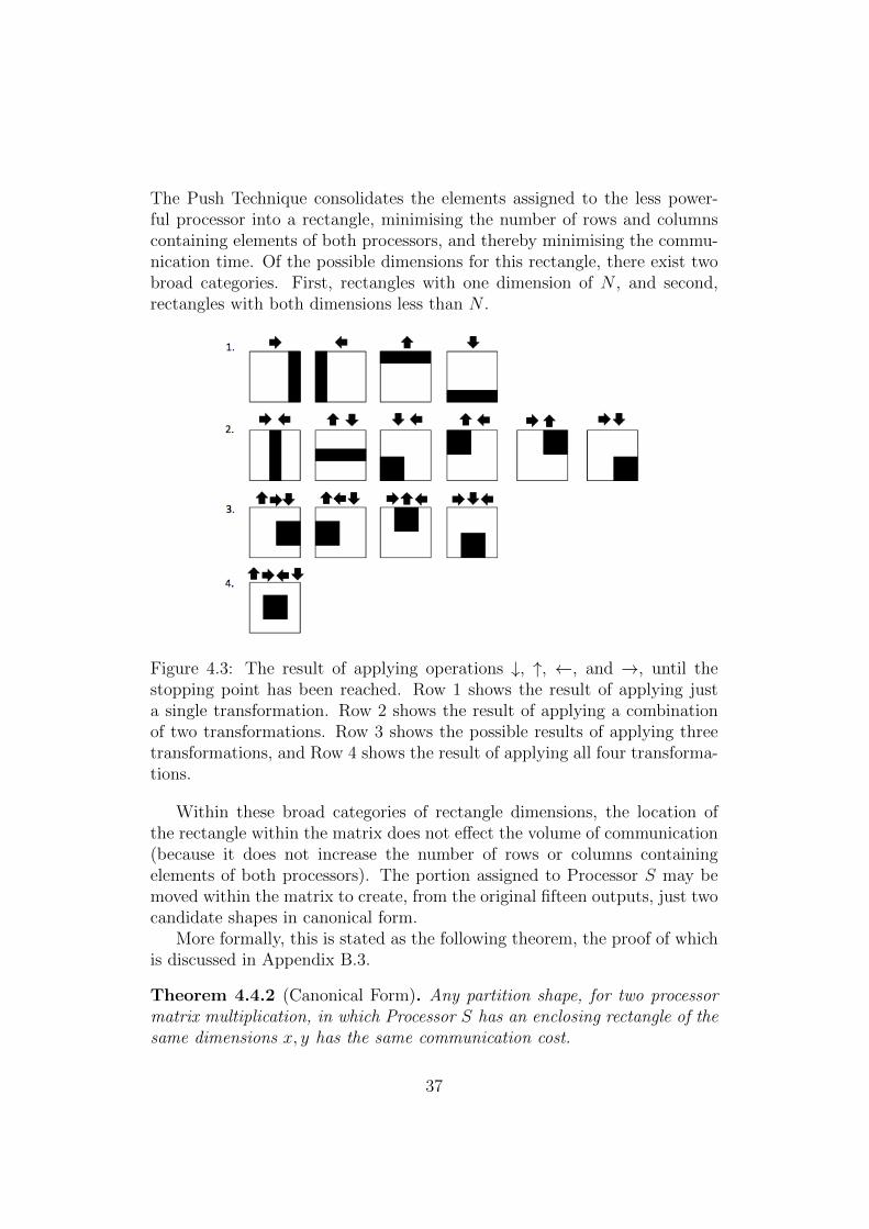
The Push Technique consolidates the elements assigned to the less power-ful processor into a rectangle, minimising the number of rows and columnscontaining elements of both processors, and thereby minimising the commu-nication time. Of the possible dimensions for this rectangle, there exist twobroad categories. First, rectangles with one dimension of N , and second,rectangles with both dimensions less than N .
Figure 4.3: The result of applying operations ↓, ↑, ←, and →, until thestopping point has been reached. Row 1 shows the result of applying justa single transformation. Row 2 shows the result of applying a combinationof two transformations. Row 3 shows the possible results of applying threetransformations, and Row 4 shows the result of applying all four transforma-tions.
Within these broad categories of rectangle dimensions, the location ofthe rectangle within the matrix does not effect the volume of communication(because it does not increase the number of rows or columns containingelements of both processors). The portion assigned to Processor S may bemoved within the matrix to create, from the original fifteen outputs, just twocandidate shapes in canonical form.
More formally, this is stated as the following theorem, the proof of whichis discussed in Appendix B.3.
Theorem 4.4.2 (Canonical Form). Any partition shape, for two processormatrix multiplication, in which Processor S has an enclosing rectangle of thesame dimensions x, y has the same communication cost.
37

The two canonical shapes are named as Straight Line and Square Cornerrespectively, and can be seen in Figure 5.1.
38
Chapter 5
Two Processor OptimalPartition Shape
The optimal partition shape for two abstract processors was a natural start-ing point for the Push Technique, which was used to create candidate optimalshapes in Chapter 4. The optimal candidates are known as Square Cornerand Straight Line.
In this chapter, the candidates are analysed to determine which is the op-timal shape. The Square Corner shape, which is non-rectangular, is shownto be optimal for a large range of ratios of processor computational power.Accordingly, the Straight Line shape, which is rectangular, is optimal for ho-mogeneous systems, and small amounts of heterogeneity in processor speed.
In the final section of this chapter, these theoretical results are confirmedexperimentally.
In order to determine which shape is optimal, first, the candidates areanalysed to determine the volume of communication each requires. Then,using the model of an abstract processor discussed in Chapter 3, perfor-mance models are built for both shapes, for each algorithm. Finally, theseperformance models are directly compared to prove mathematically whichcandidate is the optimal shape.
5.1 Optimal Candidates
Applying the Push Technique results in two potential shapes with elementsdivided between Processors P and S. In the first candidate shape ProcessorS is assigned a rectangle of length N to compute (Straight Line), and inthe second candidate shape Processor S is assigned a rectangle of less thanlength N to compute (Square Corner).
39
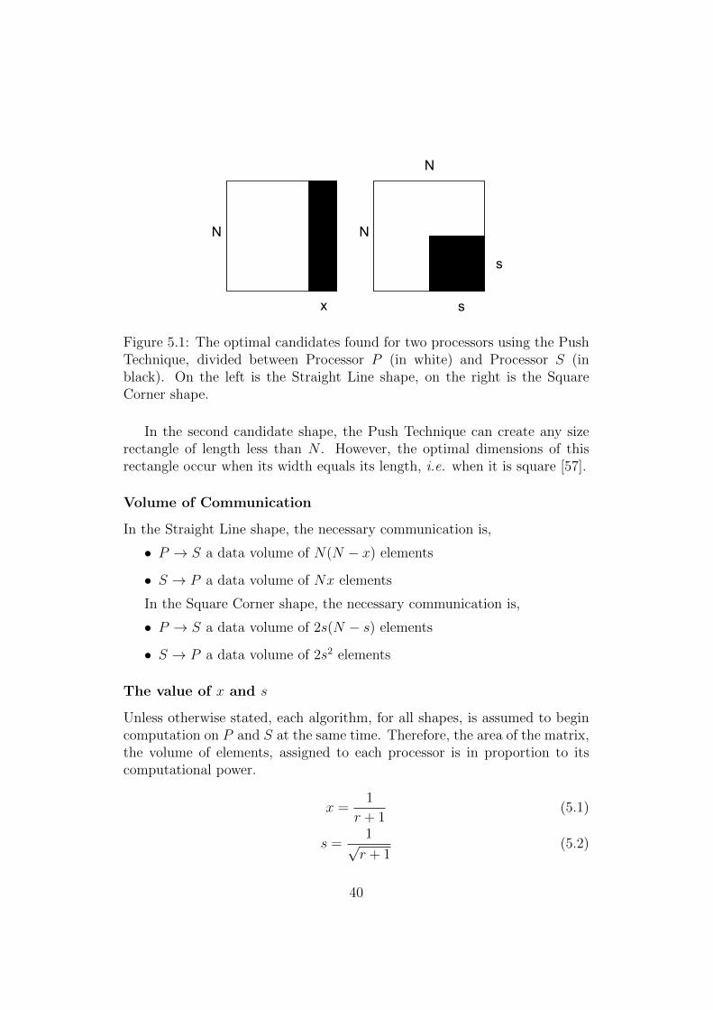
x
N
N
s
s
N
Figure 5.1: The optimal candidates found for two processors using the PushTechnique, divided between Processor P (in white) and Processor S (inblack). On the left is the Straight Line shape, on the right is the SquareCorner shape.
In the second candidate shape, the Push Technique can create any sizerectangle of length less than N . However, the optimal dimensions of thisrectangle occur when its width equals its length, i.e. when it is square [57].
Volume of Communication
In the Straight Line shape, the necessary communication is,
• P → S a data volume of N(N − x) elements
• S → P a data volume of Nx elements
In the Square Corner shape, the necessary communication is,
• P → S a data volume of 2s(N − s) elements
• S → P a data volume of 2s2 elements
The value of x and s
Unless otherwise stated, each algorithm, for all shapes, is assumed to begincomputation on P and S at the same time. Therefore, the area of the matrix,the volume of elements, assigned to each processor is in proportion to itscomputational power.
x =1
r + 1(5.1)
s =1√r + 1
(5.2)
40
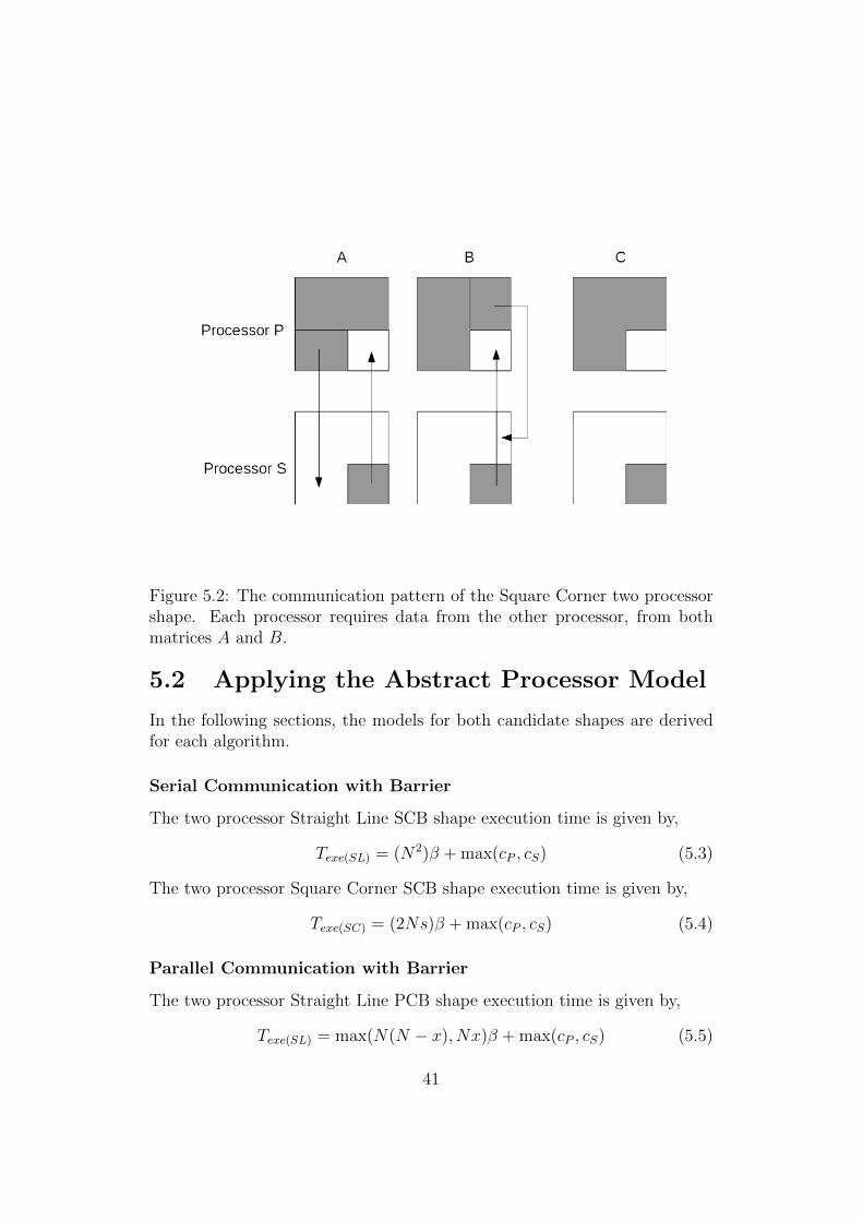
Figure 5.2: The communication pattern of the Square Corner two processorshape. Each processor requires data from the other processor, from bothmatrices A and B.
5.2 Applying the Abstract Processor Model
In the following sections, the models for both candidate shapes are derivedfor each algorithm.
Serial Communication with Barrier
The two processor Straight Line SCB shape execution time is given by,
Texe(SL) = (N2)β + max(cP , cS) (5.3)
The two processor Square Corner SCB shape execution time is given by,
Texe(SC) = (2Ns)β + max(cP , cS) (5.4)
Parallel Communication with Barrier
The two processor Straight Line PCB shape execution time is given by,
Texe(SL) = max(N(N − x), Nx)β + max(cP , cS) (5.5)
41
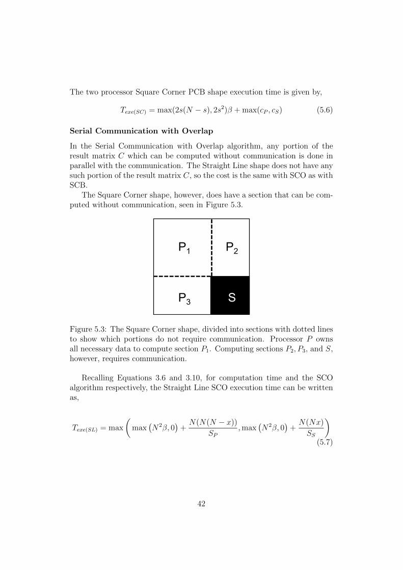
The two processor Square Corner PCB shape execution time is given by,
Texe(SC) = max(2s(N − s), 2s2)β + max(cP , cS) (5.6)
Serial Communication with Overlap
In the Serial Communication with Overlap algorithm, any portion of theresult matrix C which can be computed without communication is done inparallel with the communication. The Straight Line shape does not have anysuch portion of the result matrix C, so the cost is the same with SCO as withSCB.
The Square Corner shape, however, does have a section that can be com-puted without communication, seen in Figure 5.3.
P1 P2
P3 S
Figure 5.3: The Square Corner shape, divided into sections with dotted linesto show which portions do not require communication. Processor P ownsall necessary data to compute section P1. Computing sections P2, P3, and S,however, requires communication.
Recalling Equations 3.6 and 3.10, for computation time and the SCOalgorithm respectively, the Straight Line SCO execution time can be writtenas,
Texe(SL) = max
(max
(N2β, 0
)+N(N(N − x))
SP,max
(N2β, 0
)+N(Nx)
SS
)(5.7)
42
And the Square Corner execution time is given by,
Texe(SC) = max
(max
((2Ns)β,
N(N − s)2
SP
)+
2Ns(N − s)SP
,
max(
(2Ns)β, 0)
+N(s2)
SS
)(5.8)
These equations will be simpler to analyse after removing the constantcommon factor N3β, normalising s and x as a proportion of N so that s = s
N
and x = xN
, such that s is understood to be 0 < s < 1 (and x is understoodto be 0 < x < 1), and introducing the value c (given in Equation 3.7).
The Straight Line execution time is now (understanding the optimal sizeof x to still be 1
r+1),
Texe(SL)N3β
=1
N+
1− xc
(5.9)
The Square Corner execution is now,
Texe(SC)
N3β= max
(max
(2s
N,(1− s)2
c
)+
2(s− s2)c
,2s
N+s2r
c
)(5.10)
The Optimal Size of s for SCO. The optimal value of s is the minimum
of thisTexe(SC)
N3βon the interval of {0, 1}. However, since a value of s = 1
would indicate that Processor S has been assigned the entire matrix, theinterval of possible s values can be made more specific. The largest s will bewithout overlap is when r = 1 : 1, and therefore s = 1√
2. It has already been
established that overlap algorithms will decrease the area assigned to S, so
it can certainly be said that the optimal value of q is the minimum ofTexe(SC)
N3β
on the interval {0, 1√2}.
There are 3 functions that comprise theTexe(SC)
N3βequation. These functions
and what they represent are as follows,
y =2s
N+ 2
s− s2
c: Tcomm + (P2 + P3) (5.11)
y =(1− s)2
c+ 2
s− s2
c: P1 + (P2 + P3) (5.12)
y =2s
N+s2r
c: Tcomm + S (5.13)
The first observation is that (5.11) is always less than (5.12) on the in-terval {0, 1√
2}. Therefore, for possible values of s, it will never dominate the
maximum function and can be safely ignored. Focusing on (5.12) and (5.13),
43
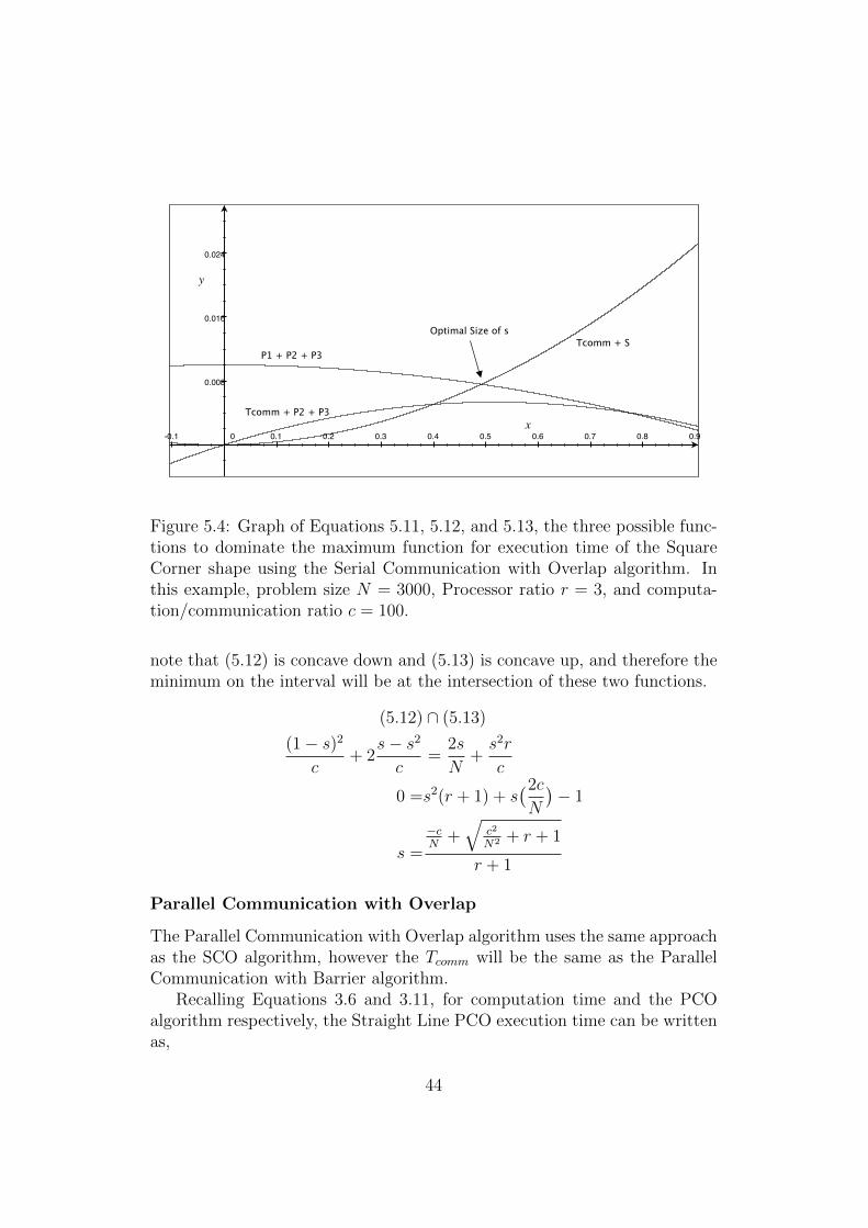
-0.1 0 0.1 0.2 0.3 0.4 0.5 0.6 0.7 0.8 0.9
0.008
0.016
0.024
Optimal Size of s
Tcomm + P2 + P3
P1 + P2 + P3Tcomm + S
Figure 5.4: Graph of Equations 5.11, 5.12, and 5.13, the three possible func-tions to dominate the maximum function for execution time of the SquareCorner shape using the Serial Communication with Overlap algorithm. Inthis example, problem size N = 3000, Processor ratio r = 3, and computa-tion/communication ratio c = 100.
note that (5.12) is concave down and (5.13) is concave up, and therefore theminimum on the interval will be at the intersection of these two functions.
(5.12) ∩ (5.13)
(1− s)2
c+ 2
s− s2
c=
2s
N+s2r
c
0 =s2(r + 1) + s(2c
N
)− 1
s =
−cN
+√
c2
N2 + r + 1
r + 1
Parallel Communication with Overlap
The Parallel Communication with Overlap algorithm uses the same approachas the SCO algorithm, however the Tcomm will be the same as the ParallelCommunication with Barrier algorithm.
Recalling Equations 3.6 and 3.11, for computation time and the PCOalgorithm respectively, the Straight Line PCO execution time can be writtenas,
44
Texe(SL) = max
(max
(max(N(N − x), Nx)β, 0
)+N(N(N − x))
SP,
max(
max(N(N − x), Nx)β, 0)
+N(Nx)
SS
)(5.14)
And the Square Corner execution time is given by,
Texe(SC) = max
(max
(max
(2s(N − s), 2s2
)β,N(N − s)2
SP
)+
2Ns(N − s)SP
,
max(
max(2s(N − s), 2s2
)β, 0)
+N(s2)
SS
)(5.15)
As with the SCO algorithm, remove the constant common factor N3β,normalise s and x as a proportion of N so that s = s
Nand x = x
N, and
introduce the value c given in Equation 3.7.The updated Straight Line execution time is given by,
Texe(SL)N3β
= max(1− x
N,x
N
)+ max
(1− xc
,rx
c
)(5.16)
And the updated Square Corner execution time is given by,
Texe(SC)
N3β= max
(max
(max
(2s− 2s2
N,2s2
N
),(1− s)2
c
)+
2(s− s2)c
,
max(2s− 2s2
N,2s2
N
)+s2r
c
)(5.17)
The Optimal Size of s for PCO. As with the SCO algorithm, theamount of the matrix assigned to Processor P in the Square Corner shape isincreased to account for the “jumpstart” that Processor P gets on computingits portion of the matrix. The optimal size to set the square of Processor S,s, is found by examining the five constituent functions which make up themaximum execution time function for this shape.
45
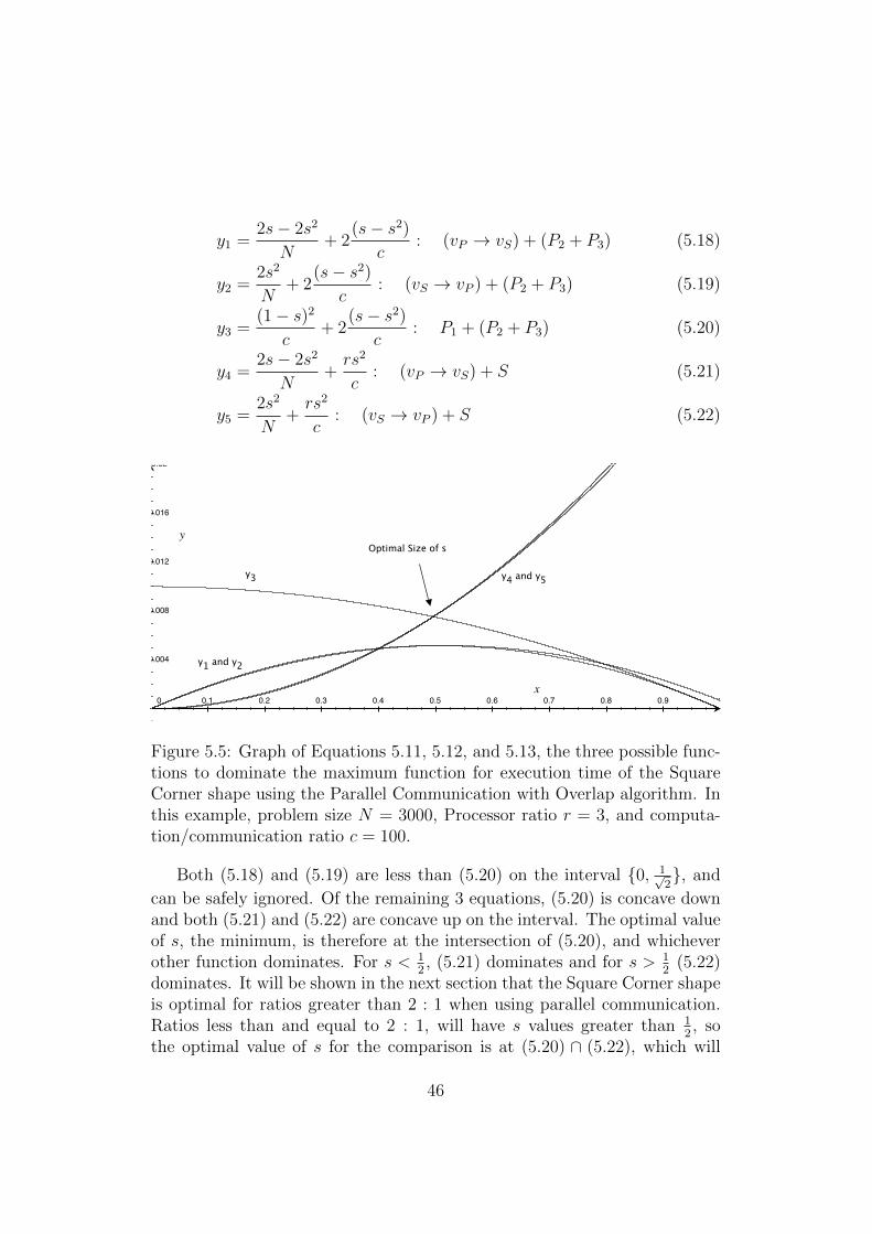
y1 =2s− 2s2
N+ 2
(s− s2)c
: (vP → vS) + (P2 + P3) (5.18)
y2 =2s2
N+ 2
(s− s2)c
: (vS → vP ) + (P2 + P3) (5.19)
y3 =(1− s)2
c+ 2
(s− s2)c
: P1 + (P2 + P3) (5.20)
y4 =2s− 2s2
N+rs2
c: (vP → vS) + S (5.21)
y5 =2s2
N+rs2
c: (vS → vP ) + S (5.22)
0 0.1 0.2 0.3 0.4 0.5 0.6 0.7 0.8 0.9 1
0.004
0.008
0.012
0.016
0.02
Optimal Size of s
y1 and y2
y3 y4 and y5
Figure 5.5: Graph of Equations 5.11, 5.12, and 5.13, the three possible func-tions to dominate the maximum function for execution time of the SquareCorner shape using the Parallel Communication with Overlap algorithm. Inthis example, problem size N = 3000, Processor ratio r = 3, and computa-tion/communication ratio c = 100.
Both (5.18) and (5.19) are less than (5.20) on the interval {0, 1√2}, and
can be safely ignored. Of the remaining 3 equations, (5.20) is concave downand both (5.21) and (5.22) are concave up on the interval. The optimal valueof s, the minimum, is therefore at the intersection of (5.20), and whicheverother function dominates. For s < 1
2, (5.21) dominates and for s > 1
2(5.22)
dominates. It will be shown in the next section that the Square Corner shapeis optimal for ratios greater than 2 : 1 when using parallel communication.Ratios less than and equal to 2 : 1, will have s values greater than 1
2, so
the optimal value of s for the comparison is at (5.20) ∩ (5.22), which will
46
give the Square Corner the optimal s value when facing the Straight Line onhomogeneous systems.
(5.20) ∩ (5.22)
(1− s)2
c+ 2
(s− s2)c
=2s2
N+rs2
c
s =1√
r + 1 + 2cN
Parallel Interleaving Overlap
For any given step k, the total amount of data being sent using this algorithmon a Square Corner partition will be s. The execution time of the SquareCorner partition is given by,
Texe(SC) = 2sβ + (N − 1) ∗max(
2sβ,N2 − s2
SP,s2
SS
)+ max
(N2 − s2
SP,s2
SS
)(5.23)
Similarly, we may use this algorithm for the Straight-Line partitioning,where the amount of data sent at each step k will be N . We define theexecution time of the Straight-Line partitioning to be given by,
Texe(SL) = Nβ+(N−1)∗max(Nβ,
N(N − x)
SP,Nx
SS
)+max
(N(N − x)
SP,Nx
SS
)(5.24)
5.3 Optimal Two Processor Data Partition
The optimal two processor matrix multiplication shape is the Square Cornerwhen the processor power ratio is
• greater than three to one (3 : 1) for SCB and PIO algorithms
• greater than two to one (2 : 1) for PCB algorithm
• for all ratios for SCO and PCO algorithms
For all other ratios the Straight Line shape is the optimal. These resultswere previously published in [57]. The proofs for these claims follow.
47
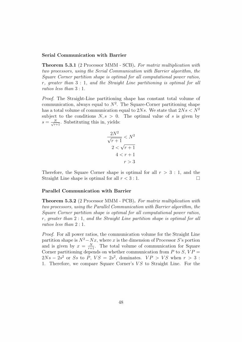
Serial Communication with Barrier
Theorem 5.3.1 (2 Processor MMM - SCB). For matrix multiplication withtwo processors, using the Serial Communication with Barrier algorithm, theSquare Corner partition shape is optimal for all computational power ratios,r, greater than 3 : 1, and the Straight Line partitioning is optimal for allratios less than 3 : 1.
Proof. The Straight-Line partitioning shape has constant total volume ofcommunication, always equal to N2. The Square-Corner partitioning shapehas a total volume of communication equal to 2Ns. We state that 2Ns < N2
subject to the conditions N, s > 0. The optimal value of s is given bys = N√
r+1. Substituting this in, yields:
2N2
√r + 1
< N2
2 <√r + 1
4 < r + 1
r > 3
Therefore, the Square Corner shape is optimal for all r > 3 : 1, and theStraight Line shape is optimal for all r < 3 : 1.
Parallel Communication with Barrier
Theorem 5.3.2 (2 Processor MMM - PCB). For matrix multiplication withtwo processors, using the Parallel Communication with Barrier algorithm, theSquare Corner partition shape is optimal for all computational power ratios,r, greater than 2 : 1, and the Straight Line partition shape is optimal for allratios less than 2 : 1.
Proof. For all power ratios, the communication volume for the Straight Linepartition shape is N2−Nx, where x is the dimension of Processor S’s portionand is given by x = N
r+1. The total volume of communication for Square
Corner partitioning depends on whether communication from P to S, V P =2Ns − 2s2 or Ss to P , V S = 2s2, dominates. V P > V S when r > 3 :1. Therefore, we compare Square Corner’s V S to Straight Line. For the
48
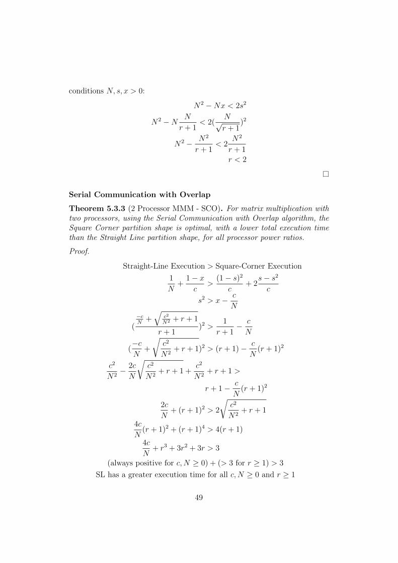
conditions N, s, x > 0:
N2 −Nx < 2s2
N2 −N N
r + 1< 2(
N√r + 1
)2
N2 − N2
r + 1< 2
N2
r + 1
r < 2
Serial Communication with Overlap
Theorem 5.3.3 (2 Processor MMM - SCO). For matrix multiplication withtwo processors, using the Serial Communication with Overlap algorithm, theSquare Corner partition shape is optimal, with a lower total execution timethan the Straight Line partition shape, for all processor power ratios.
Proof.
Straight-Line Execution > Square-Corner Execution
1
N+
1− xc
>(1− s)2
c+ 2
s− s2
c
s2 > x− c
N
(
−cN
+√
c2
N2 + r + 1
r + 1)2 >
1
r + 1− c
N
(−cN
+
√c2
N2+ r + 1)2 > (r + 1)− c
N(r + 1)2
c2
N2− 2c
N
√c2
N2+ r + 1 +
c2
N2+ r + 1 >
r + 1− c
N(r + 1)2
2c
N+ (r + 1)2 > 2
√c2
N2+ r + 1
4c
N(r + 1)2 + (r + 1)4 > 4(r + 1)
4c
N+ r3 + 3r2 + 3r > 3
(always positive for c,N ≥ 0) + (> 3 for r ≥ 1) > 3
SL has a greater execution time for all c,N ≥ 0 and r ≥ 1
49
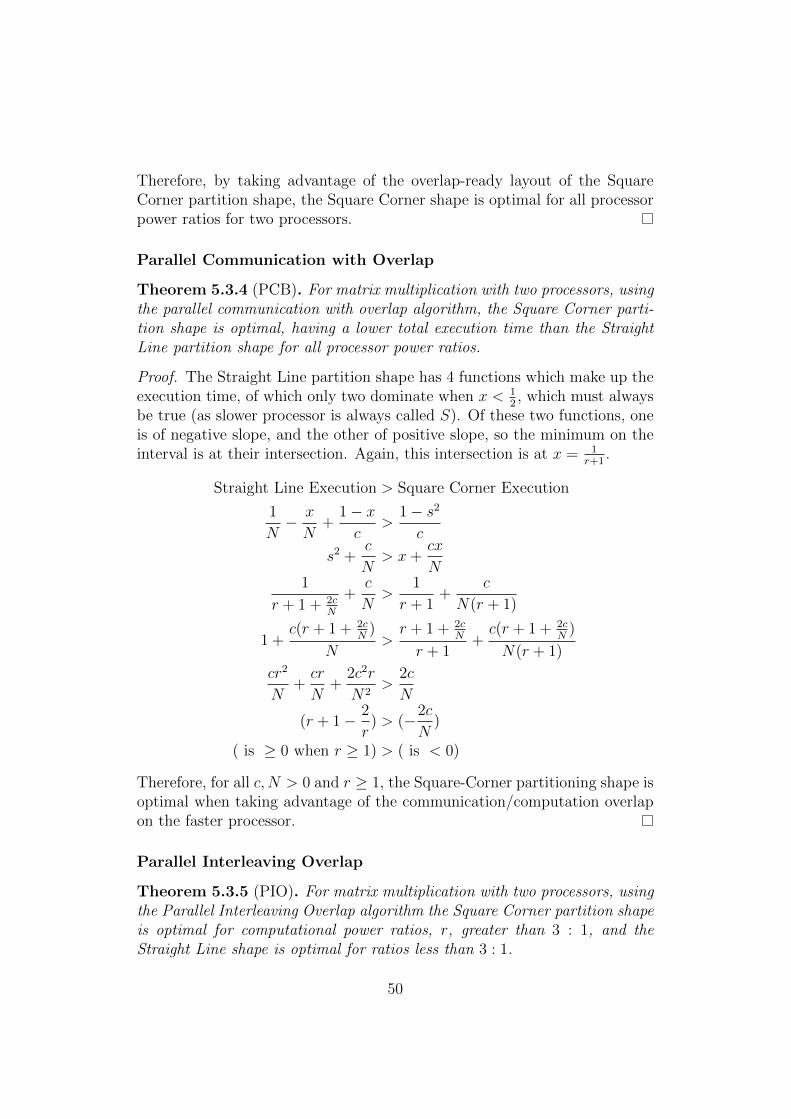
Therefore, by taking advantage of the overlap-ready layout of the SquareCorner partition shape, the Square Corner shape is optimal for all processorpower ratios for two processors.
Parallel Communication with Overlap
Theorem 5.3.4 (PCB). For matrix multiplication with two processors, usingthe parallel communication with overlap algorithm, the Square Corner parti-tion shape is optimal, having a lower total execution time than the StraightLine partition shape for all processor power ratios.
Proof. The Straight Line partition shape has 4 functions which make up theexecution time, of which only two dominate when x < 1
2, which must always
be true (as slower processor is always called S). Of these two functions, oneis of negative slope, and the other of positive slope, so the minimum on theinterval is at their intersection. Again, this intersection is at x = 1
r+1.
Straight Line Execution > Square Corner Execution
1
N− x
N+
1− xc
>1− s2
c
s2 +c
N> x+
cx
N1
r + 1 + 2cN
+c
N>
1
r + 1+
c
N(r + 1)
1 +c(r + 1 + 2c
N)
N>r + 1 + 2c
N
r + 1+c(r + 1 + 2c
N)
N(r + 1)
cr2
N+cr
N+
2c2r
N2>
2c
N
(r + 1− 2
r) > (−2c
N)
( is ≥ 0 when r ≥ 1) > ( is < 0)
Therefore, for all c,N > 0 and r ≥ 1, the Square-Corner partitioning shape isoptimal when taking advantage of the communication/computation overlapon the faster processor.
Parallel Interleaving Overlap
Theorem 5.3.5 (PIO). For matrix multiplication with two processors, usingthe Parallel Interleaving Overlap algorithm the Square Corner partition shapeis optimal for computational power ratios, r, greater than 3 : 1, and theStraight Line shape is optimal for ratios less than 3 : 1.
50
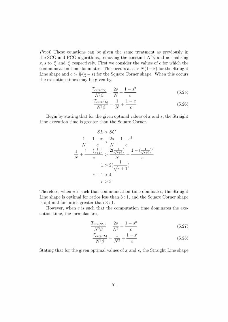
Proof. These equations can be given the same treatment as previously inthe SCO and PCO algorithms, removing the constant N3β and normalisingx, s to x
Nand s
Nrespectively. First we consider the values of c for which the
communication time dominates. This occurs at c > N(1−x) for the StraightLine shape and c > N
2(1s− s) for the Square Corner shape. When this occurs
the execution times may be given by,
Texe(SC)
N3β=
2s
N+
1− s2
c(5.25)
Texe(SL)N3β
=1
N+
1− xc
(5.26)
Begin by stating that for the given optimal values of x and s, the StraightLine execution time is greater than the Square Corner,
SL > SC
1
N+
1− xc
>2s
N+
1− s2
c
1
N+
1− ( 1r+1
)
c>
2( 1√r+1
)
N+
1− ( 1√r+1
)2
c
1 > 2(1√r + 1
)
r + 1 > 4
r > 3
Therefore, when c is such that communication time dominates, the StraightLine shape is optimal for ratios less than 3 : 1, and the Square Corner shapeis optimal for ratios greater than 3 : 1.
However, when c is such that the computation time dominates the exe-cution time, the formulas are,
Texe(SC)
N3β=
2s
N2+
1− s2
c(5.27)
Texe(SL)N3β
=1
N2+
1− xc
(5.28)
Stating that for the given optimal values of x and s, the Straight Line shape
51
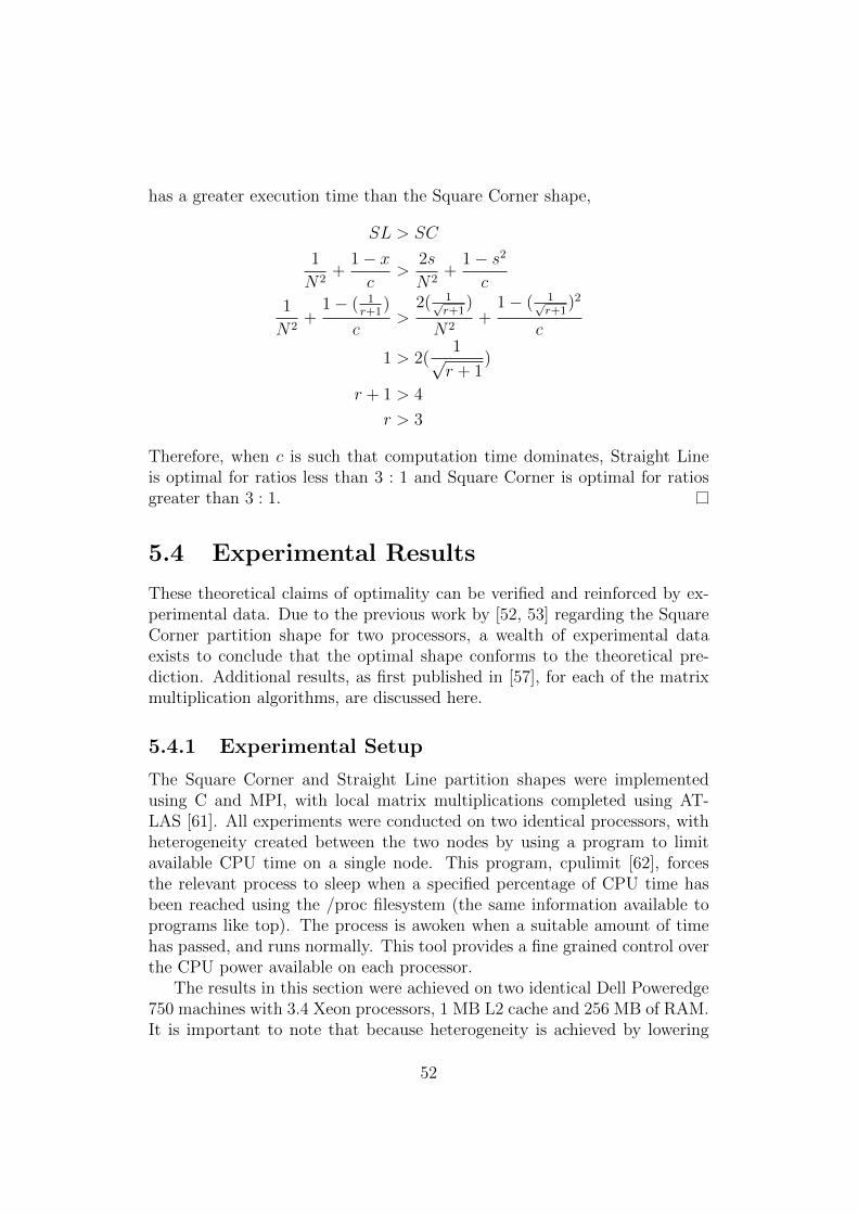
has a greater execution time than the Square Corner shape,
SL > SC
1
N2+
1− xc
>2s
N2+
1− s2
c
1
N2+
1− ( 1r+1
)
c>
2( 1√r+1
)
N2+
1− ( 1√r+1
)2
c
1 > 2(1√r + 1
)
r + 1 > 4
r > 3
Therefore, when c is such that computation time dominates, Straight Lineis optimal for ratios less than 3 : 1 and Square Corner is optimal for ratiosgreater than 3 : 1.
5.4 Experimental Results
These theoretical claims of optimality can be verified and reinforced by ex-perimental data. Due to the previous work by [52, 53] regarding the SquareCorner partition shape for two processors, a wealth of experimental dataexists to conclude that the optimal shape conforms to the theoretical pre-diction. Additional results, as first published in [57], for each of the matrixmultiplication algorithms, are discussed here.
5.4.1 Experimental Setup
The Square Corner and Straight Line partition shapes were implementedusing C and MPI, with local matrix multiplications completed using AT-LAS [61]. All experiments were conducted on two identical processors, withheterogeneity created between the two nodes by using a program to limitavailable CPU time on a single node. This program, cpulimit [62], forcesthe relevant process to sleep when a specified percentage of CPU time hasbeen reached using the /proc filesystem (the same information available toprograms like top). The process is awoken when a suitable amount of timehas passed, and runs normally. This tool provides a fine grained control overthe CPU power available on each processor.
The results in this section were achieved on two identical Dell Poweredge750 machines with 3.4 Xeon processors, 1 MB L2 cache and 256 MB of RAM.It is important to note that because heterogeneity is achieved by lowering
52
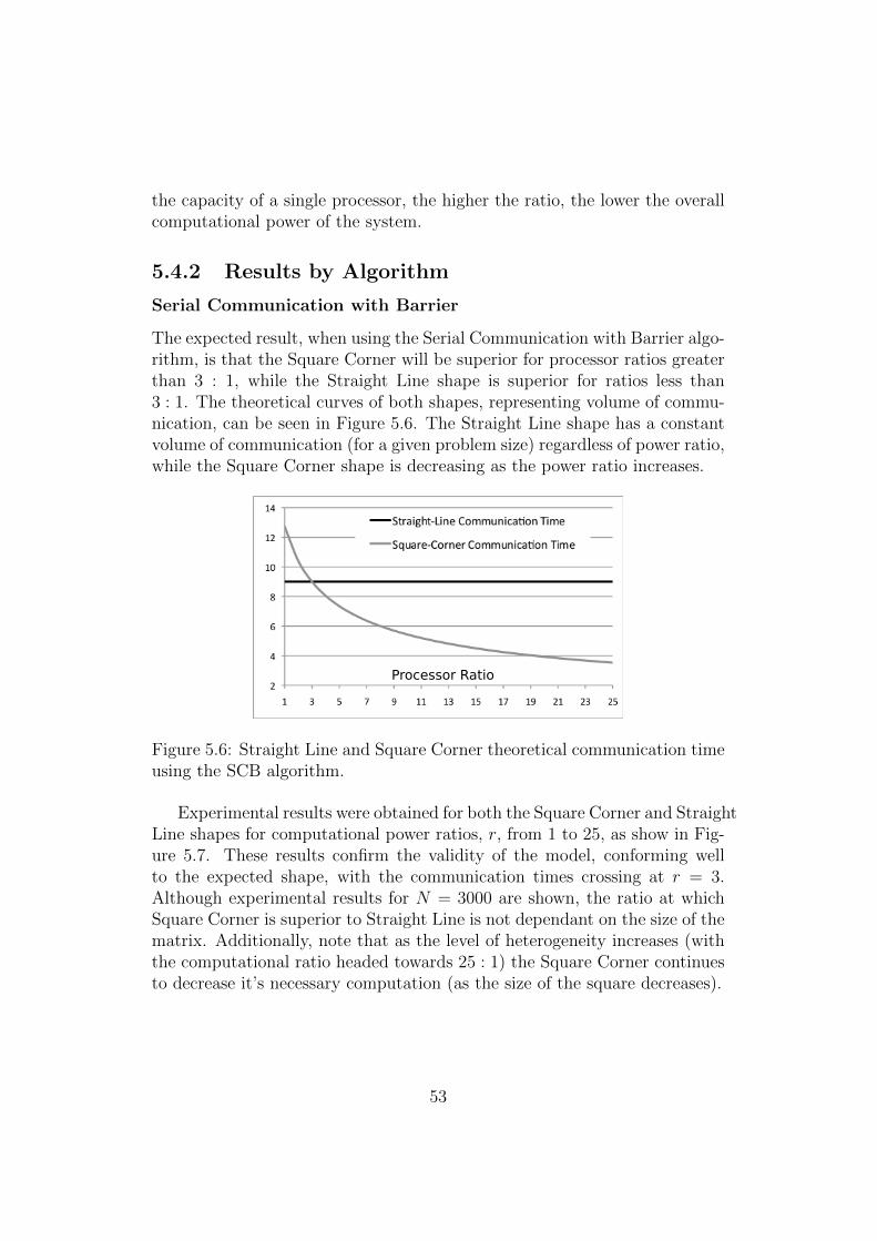
the capacity of a single processor, the higher the ratio, the lower the overallcomputational power of the system.
5.4.2 Results by Algorithm
Serial Communication with Barrier
The expected result, when using the Serial Communication with Barrier algo-rithm, is that the Square Corner will be superior for processor ratios greaterthan 3 : 1, while the Straight Line shape is superior for ratios less than3 : 1. The theoretical curves of both shapes, representing volume of commu-nication, can be seen in Figure 5.6. The Straight Line shape has a constantvolume of communication (for a given problem size) regardless of power ratio,while the Square Corner shape is decreasing as the power ratio increases.
Processor Ratio
Figure 5.6: Straight Line and Square Corner theoretical communication timeusing the SCB algorithm.
Experimental results were obtained for both the Square Corner and StraightLine shapes for computational power ratios, r, from 1 to 25, as show in Fig-ure 5.7. These results confirm the validity of the model, conforming wellto the expected shape, with the communication times crossing at r = 3.Although experimental results for N = 3000 are shown, the ratio at whichSquare Corner is superior to Straight Line is not dependant on the size of thematrix. Additionally, note that as the level of heterogeneity increases (withthe computational ratio headed towards 25 : 1) the Square Corner continuesto decrease it’s necessary computation (as the size of the square decreases).
53
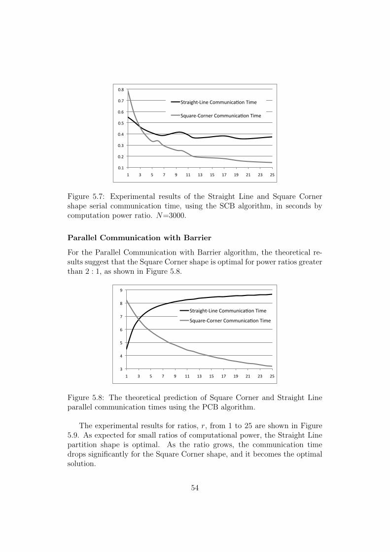
0.1
0.2
0.3
0.4
0.5
0.6
0.7
0.8
1 3 5 7 9 11 13 15 17 19 21 23 25
Straight‐LineCommunica=onTime
Square‐CornerCommunica=onTime
Figure 5.7: Experimental results of the Straight Line and Square Cornershape serial communication time, using the SCB algorithm, in seconds bycomputation power ratio. N=3000.
Parallel Communication with Barrier
For the Parallel Communication with Barrier algorithm, the theoretical re-sults suggest that the Square Corner shape is optimal for power ratios greaterthan 2 : 1, as shown in Figure 5.8.
3
4
5
6
7
8
9
1 3 5 7 9 11 13 15 17 19 21 23 25
Straight‐LineCommunica;onTime
Square‐CornerCommunica;onTime
Figure 5.8: The theoretical prediction of Square Corner and Straight Lineparallel communication times using the PCB algorithm.
The experimental results for ratios, r, from 1 to 25 are shown in Figure5.9. As expected for small ratios of computational power, the Straight Linepartition shape is optimal. As the ratio grows, the communication timedrops significantly for the Square Corner shape, and it becomes the optimalsolution.
54
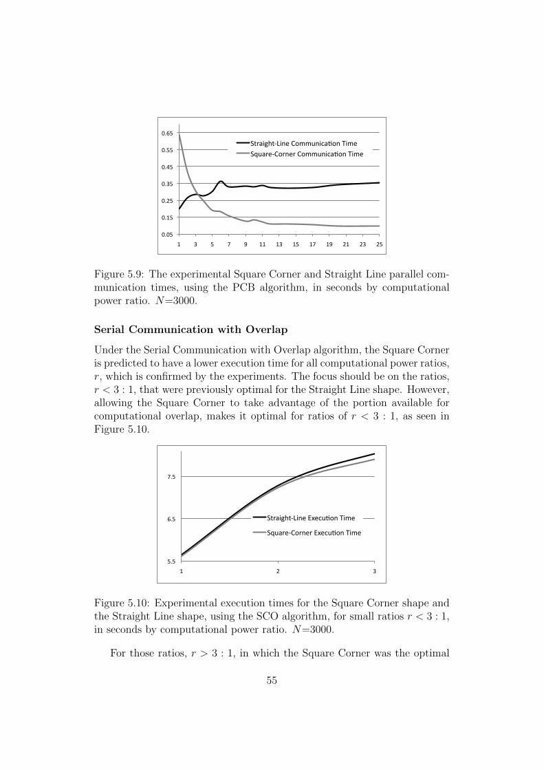
0.05
0.15
0.25
0.35
0.45
0.55
0.65
1 3 5 7 9 11 13 15 17 19 21 23 25
Straight‐LineCommunica<onTimeSquare‐CornerCommunica<onTime
Figure 5.9: The experimental Square Corner and Straight Line parallel com-munication times, using the PCB algorithm, in seconds by computationalpower ratio. N=3000.
Serial Communication with Overlap
Under the Serial Communication with Overlap algorithm, the Square Corneris predicted to have a lower execution time for all computational power ratios,r, which is confirmed by the experiments. The focus should be on the ratios,r < 3 : 1, that were previously optimal for the Straight Line shape. However,allowing the Square Corner to take advantage of the portion available forcomputational overlap, makes it optimal for ratios of r < 3 : 1, as seen inFigure 5.10.
5.5
6.5
7.5
1 2 3
Straight‐LineExecu8onTime
Square‐CornerExecu8onTime
Figure 5.10: Experimental execution times for the Square Corner shape andthe Straight Line shape, using the SCO algorithm, for small ratios r < 3 : 1,in seconds by computational power ratio. N=3000.
For those ratios, r > 3 : 1, in which the Square Corner was the optimal
55
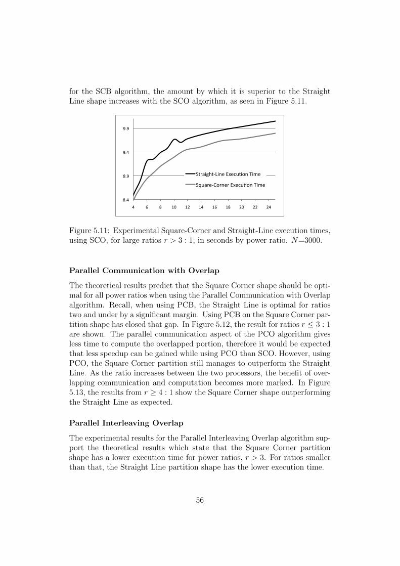
for the SCB algorithm, the amount by which it is superior to the StraightLine shape increases with the SCO algorithm, as seen in Figure 5.11.
8.4
8.9
9.4
9.9
4 6 8 10 12 14 16 18 20 22 24
Straight‐LineExecu9onTime
Square‐CornerExecu9onTime
Figure 5.11: Experimental Square-Corner and Straight-Line execution times,using SCO, for large ratios r > 3 : 1, in seconds by power ratio. N=3000.
Parallel Communication with Overlap
The theoretical results predict that the Square Corner shape should be opti-mal for all power ratios when using the Parallel Communication with Overlapalgorithm. Recall, when using PCB, the Straight Line is optimal for ratiostwo and under by a significant margin. Using PCB on the Square Corner par-tition shape has closed that gap. In Figure 5.12, the result for ratios r ≤ 3 : 1are shown. The parallel communication aspect of the PCO algorithm givesless time to compute the overlapped portion, therefore it would be expectedthat less speedup can be gained while using PCO than SCO. However, usingPCO, the Square Corner partition still manages to outperform the StraightLine. As the ratio increases between the two processors, the benefit of over-lapping communication and computation becomes more marked. In Figure5.13, the results from r ≥ 4 : 1 show the Square Corner shape outperformingthe Straight Line as expected.
Parallel Interleaving Overlap
The experimental results for the Parallel Interleaving Overlap algorithm sup-port the theoretical results which state that the Square Corner partitionshape has a lower execution time for power ratios, r > 3. For ratios smallerthan that, the Straight Line partition shape has the lower execution time.
56
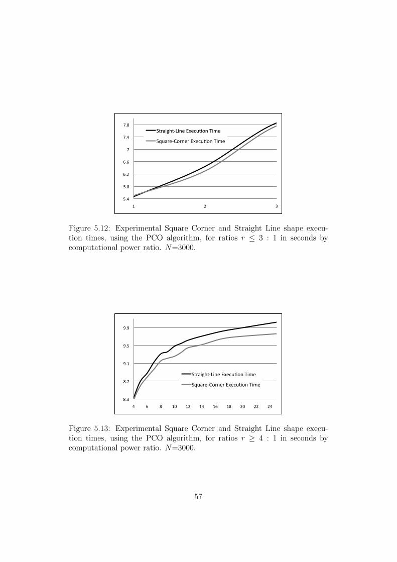
5.4
5.8
6.2
6.6
7
7.4
7.8
1 2 3
Straight‐LineExecu:onTime
Square‐CornerExecu:onTime
Figure 5.12: Experimental Square Corner and Straight Line shape execu-tion times, using the PCO algorithm, for ratios r ≤ 3 : 1 in seconds bycomputational power ratio. N=3000.
8.3
8.7
9.1
9.5
9.9
4 6 8 10 12 14 16 18 20 22 24
Straight‐LineExecu<onTime
Square‐CornerExecu<onTime
Figure 5.13: Experimental Square Corner and Straight Line shape execu-tion times, using the PCO algorithm, for ratios r ≥ 4 : 1 in seconds bycomputational power ratio. N=3000.
57
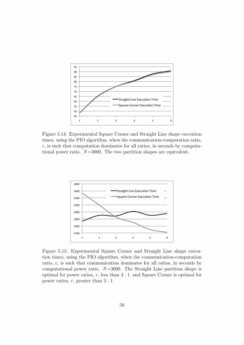
45
50
55
60
65
70
75
80
85
90
95
1 2 3 4 5 6
Straight‐LineExecu;onTime
Square‐CornerExecu;onTime
Figure 5.14: Experimental Square Corner and Straight Line shape executiontimes, using the PIO algorithm, when the communication-computation ratio,c, is such that computation dominates for all ratios, in seconds by computa-tional power ratio. N=3000. The two partition shapes are equivalent.
1400
1600
1800
2000
2200
2400
2600
2800
1 2 3 4 5 6
Straight‐LineExecu9onTime
Square‐CornerExecu9onTime
Figure 5.15: Experimental Square Corner and Straight Line shape execu-tion times, using the PIO algorithm, when the communication-computationratio, c, is such that communication dominates for all ratios, in seconds bycomputational power ratio. N=3000. The Straight Line partition shape isoptimal for power ratios, r, less than 3 : 1, and Square Corner is optimal forpower ratios, r, greater than 3 : 1.
58
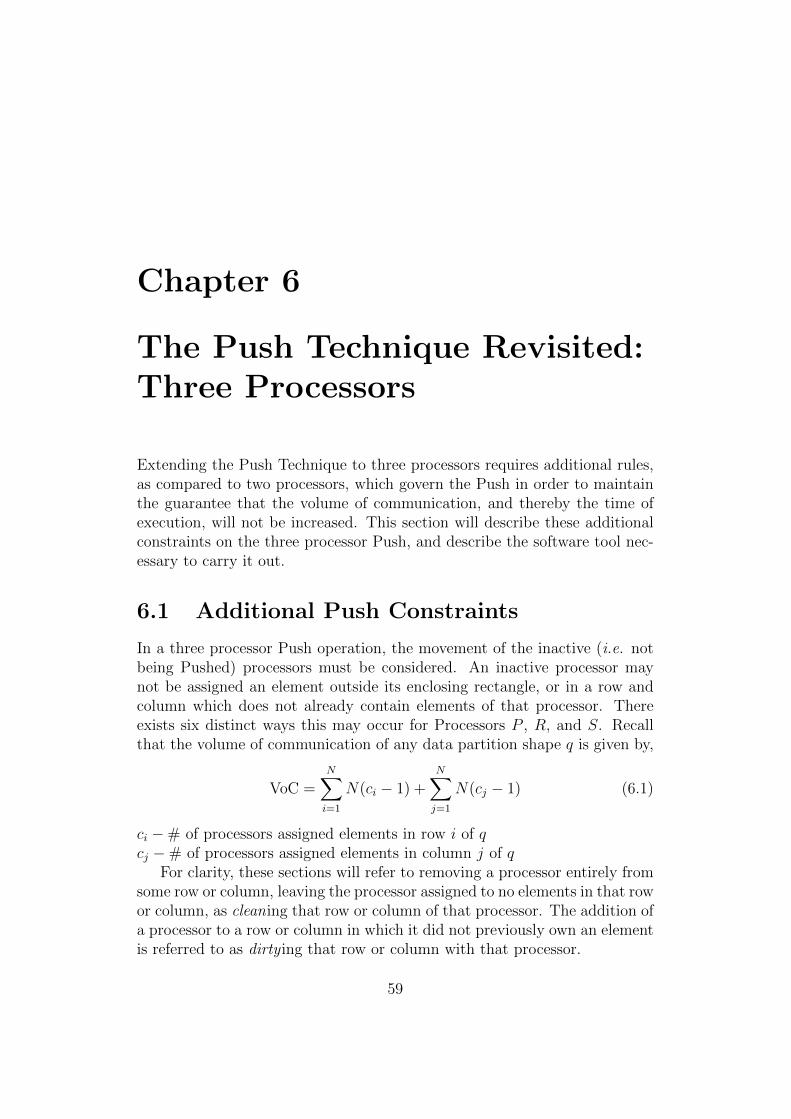
Chapter 6
The Push Technique Revisited:Three Processors
Extending the Push Technique to three processors requires additional rules,as compared to two processors, which govern the Push in order to maintainthe guarantee that the volume of communication, and thereby the time ofexecution, will not be increased. This section will describe these additionalconstraints on the three processor Push, and describe the software tool nec-essary to carry it out.
6.1 Additional Push Constraints
In a three processor Push operation, the movement of the inactive (i.e. notbeing Pushed) processors must be considered. An inactive processor maynot be assigned an element outside its enclosing rectangle, or in a row andcolumn which does not already contain elements of that processor. Thereexists six distinct ways this may occur for Processors P , R, and S. Recallthat the volume of communication of any data partition shape q is given by,
VoC =N∑i=1
N(ci − 1) +N∑j=1
N(cj − 1) (6.1)
ci −# of processors assigned elements in row i of qcj −# of processors assigned elements in column j of q
For clarity, these sections will refer to removing a processor entirely fromsome row or column, leaving the processor assigned to no elements in that rowor column, as cleaning that row or column of that processor. The addition ofa processor to a row or column in which it did not previously own an elementis referred to as dirty ing that row or column with that processor.
59
These descriptions assume the chosen input to the Push DFA is a PushDown (↓) on Processor R, but are similar for other directions and Pushoperations on Processor S.
Type One - Decreases Volume of Communication
For each element assigned to Processor R in rtop, Processor R is assignedan element in the below rows and columns already containing elements ofProcessor R.
For each element which has been reassigned to R, the Processor previouslyassigned that element is given some unassigned element (rtop, j). Prior to thePush, this Processor must have already had an element in row rtop and incolumn j.
Type Two - Decreases Volume of Communication
For each element assigned to Processor R in rtop, Processor R is assignedan element in the rows below. Elements may go to some number, l, of rowsand columns which did not already contain elements of Processor R, dirty ingthose rows and columns, if l or more rows and columns are also cleaned ofR.
For each element which has been reassigned to R, the Processor previouslyassigned that element is given some unassigned element (rtop, j). Prior to thePush, this processor must already have had an element in row rtop and incolumn j.
Type Three - Decreases Volume of Communication
For each element assigned to Processor R in rtop, Processor R is assignedan element in the rows and columns below that already contain elements ofProcessor R.
For each element which has been reassigned to R, the Processor previouslyassigned that element is given some unassigned element (rtop, j). Prior to thePush, it is not necessary for this Processor to have had an element in rtopor j, provided the number of rows and columns dirtied, l, is less than thenumber of rows and columns cleaned.
Type Four - Decreases Volume of Communication
For each element assigned to Processor R in rtop, Processor R is assigned anelement in the rows below. Elements may go to some number of rows andcolumns, l, which did not already contain elements of Processor R, dirtying
60
those rows and columns, if l or more rows and columns are also cleaned ofR.
For each element which has been reassigned to R, the Processor previouslyassigned that element is given some unassigned element (rtop, j). Prior to thePush, it is not necessary that this Processor have already had an element inrtop or j, provided the number of rows and columns dirtied, l, is less than thenumber of rows and columns cleaned.
Type Five - Unchanged Volume of Communication
For each element assigned to Processor R in rtop, Processor R is assigned anelement in the rows below. A single row or column not containing elementsof Processor R may be dirtied.
For each element which has been reassigned to R, the Processor previouslyassigned that element is given some unassigned element (rtop, j). Prior to thePush, this Processor must have been assigned an element in row rtop and incolumn j.
Type Six- Unchanged/Decrease Volume of Communication
For each element assigned to Processor R in rtop, Processor R is assigned anelement in the rows below. A single row or column not containing elementsof Processor R may be dirtied.
For each element which has been reassigned to R, the Processor previouslyassigned that element is given some unassigned element (rtop, j). Prior to thePush, it is not necessary that this Processor have had an element in rtop orj, provided the number of rows and columns dirtied, l, is less than or equalto the number of rows and columns cleaned.
6.2 Implementing the Push DFA
In order to show that the three processor Push always converges on somesmall set of candidates, the DFA was implemented as a software tool. Thissection describes the design and implementation of the tool, as well as thepractical outcomes of its use.
6.2.1 Motivation
Generally, when proving mathematical concepts, the grand idea is alreadyfixed in mind, and equations are tools used to convince others of the veracityof the big idea. The more complex nature of the three processor Push does
61
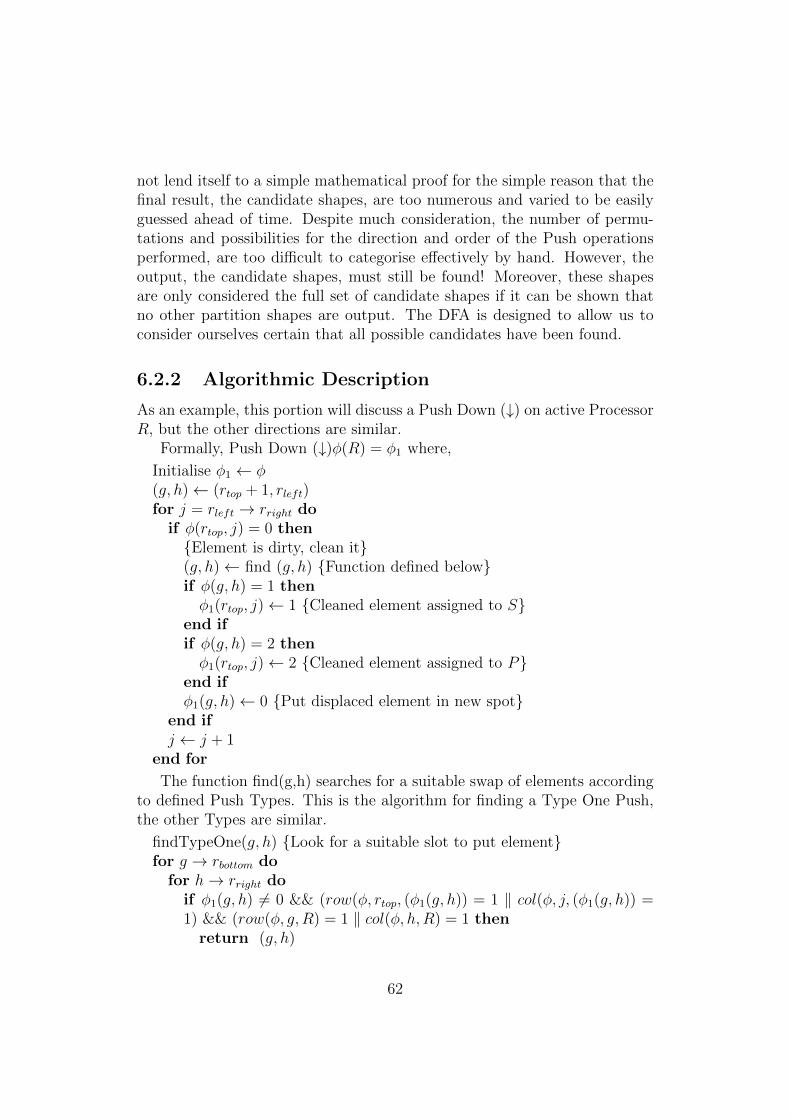
not lend itself to a simple mathematical proof for the simple reason that thefinal result, the candidate shapes, are too numerous and varied to be easilyguessed ahead of time. Despite much consideration, the number of permu-tations and possibilities for the direction and order of the Push operationsperformed, are too difficult to categorise effectively by hand. However, theoutput, the candidate shapes, must still be found! Moreover, these shapesare only considered the full set of candidate shapes if it can be shown thatno other partition shapes are output. The DFA is designed to allow us toconsider ourselves certain that all possible candidates have been found.
6.2.2 Algorithmic Description
As an example, this portion will discuss a Push Down (↓) on active ProcessorR, but the other directions are similar.
Formally, Push Down (↓)φ(R) = φ1 where,
Initialise φ1 ← φ(g, h)← (rtop + 1, rleft)for j = rleft → rright do
if φ(rtop, j) = 0 then{Element is dirty, clean it}(g, h)← find (g, h) {Function defined below}if φ(g, h) = 1 thenφ1(rtop, j)← 1 {Cleaned element assigned to S}
end ifif φ(g, h) = 2 thenφ1(rtop, j)← 2 {Cleaned element assigned to P}
end ifφ1(g, h)← 0 {Put displaced element in new spot}
end ifj ← j + 1
end for
The function find(g,h) searches for a suitable swap of elements accordingto defined Push Types. This is the algorithm for finding a Type One Push,the other Types are similar.
findTypeOne(g, h) {Look for a suitable slot to put element}for g → rbottom do
for h→ rright doif φ1(g, h) 6= 0 && (row(φ, rtop, (φ1(g, h)) = 1 ‖ col(φ, j, (φ1(g, h)) =1) && (row(φ, g, R) = 1 ‖ col(φ, h,R) = 1 then
return (g, h)
62
end ifh← h+ 1
end forh← kleftg ← g + 1
end forreturn φ1 = φ {No Type One Push↓ φ(R) possible}
6.2.3 End Conditions
In order to implement the Push, there must exist strictly defined conditionsunder which a partition is considered fully Pushed. In the theoretical Push,a partition is considered fully Pushed, or condensed, when the elements of noprocessors, except the largest processor, may be legally moved in any Pushdirection.
The implementation of the DFA program first determines the valid di-rections of Push for a given processor in a given run. A partition is fullycondensed if there are no available Push operations in those predetermineddirections.
6.3 Experimental Results with the Push DFA
This section describes the use of the Push DFA to collect all possible candi-date partition shapes for further analysis. The results of these experimentswere previously published in [63].
6.3.1 Experimental Setup
The size of the matrix chosen must be large enough to possess the granularityof elements required to form a variety of shapes, and be considered represen-tative of any value of N . However, the larger the matrix size N , the largerthe set of possible states, Q, and therefore more experimental runs are nec-essary to appropriately cover them all. To balance these two requirements,N = 1000 was chosen.
The processor ratios chosen for study were 2:1:1, 3:1:1, 4:1:1, 5:1:1, 10:1:1,10:5:1, 10:8:1 2:2:1, 3:2:1, 4:2:1, 5:2:1, 5:3:1, 5:4:1. For each ratio, the DFAimplementation was run approximately 10,000 times. The DFA is not a sim-ulation of actual matrix multiplication on parallel processors, but searchingfor partition shapes which cannot be improved using the Push operation,so it is designed to be run on a single processor. Multiple instances of the
63
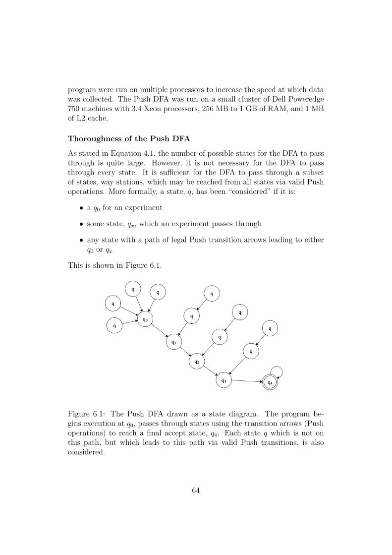
program were run on multiple processors to increase the speed at which datawas collected. The Push DFA was run on a small cluster of Dell Poweredge750 machines with 3.4 Xeon processors, 256 MB to 1 GB of RAM, and 1 MBof L2 cache.
Thoroughness of the Push DFA
As stated in Equation 4.1, the number of possible states for the DFA to passthrough is quite large. However, it is not necessary for the DFA to passthrough every state. It is sufficient for the DFA to pass through a subsetof states, way stations, which may be reached from all states via valid Pushoperations. More formally, a state, q, has been “considered” if it is:
• a q0 for an experiment
• some state, qx, which an experiment passes through
• any state with a path of legal Push transition arrows leading to eitherq0 or qx
This is shown in Figure 6.1.
Figure 6.1: The Push DFA drawn as a state diagram. The program be-gins execution at q0, passes through states using the transition arrows (Pushoperations) to reach a final accept state, q4. Each state q which is not onthis path, but which leads to this path via valid Push transitions, is alsoconsidered.
64
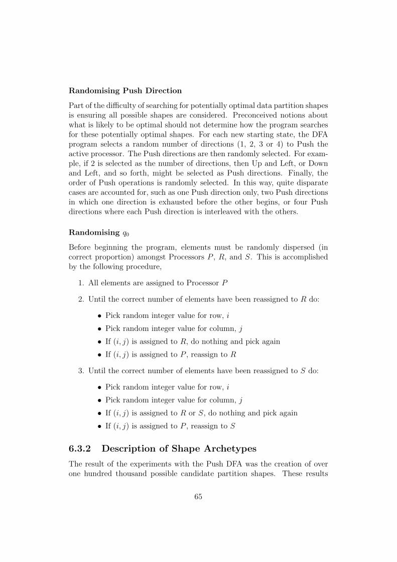
Randomising Push Direction
Part of the difficulty of searching for potentially optimal data partition shapesis ensuring all possible shapes are considered. Preconceived notions aboutwhat is likely to be optimal should not determine how the program searchesfor these potentially optimal shapes. For each new starting state, the DFAprogram selects a random number of directions (1, 2, 3 or 4) to Push theactive processor. The Push directions are then randomly selected. For exam-ple, if 2 is selected as the number of directions, then Up and Left, or Downand Left, and so forth, might be selected as Push directions. Finally, theorder of Push operations is randomly selected. In this way, quite disparatecases are accounted for, such as one Push direction only, two Push directionsin which one direction is exhausted before the other begins, or four Pushdirections where each Push direction is interleaved with the others.
Randomising q0
Before beginning the program, elements must be randomly dispersed (incorrect proportion) amongst Processors P , R, and S. This is accomplishedby the following procedure,
1. All elements are assigned to Processor P
2. Until the correct number of elements have been reassigned to R do:
• Pick random integer value for row, i
• Pick random integer value for column, j
• If (i, j) is assigned to R, do nothing and pick again
• If (i, j) is assigned to P , reassign to R
3. Until the correct number of elements have been reassigned to S do:
• Pick random integer value for row, i
• Pick random integer value for column, j
• If (i, j) is assigned to R or S, do nothing and pick again
• If (i, j) is assigned to P , reassign to S
6.3.2 Description of Shape Archetypes
The result of the experiments with the Push DFA was the creation of overone hundred thousand possible candidate partition shapes. These results
65
A B C D
Figure 6.2: The general partition shape archetypes found experimentally bythe Push DFA. Each shape archetype includes all possible shapes with thesame characteristics of overlap of enclosing rectangles, and number of cornerspresent.
were parsed and categorised according to two distinct metrics, the relativeposition of the enclosing rectangles, and the number of corners present ineach processor’s shape. This resulted in four broad categories, called ShapeArchetypes, in which all shapes output by the DFA fit. These archetypes,called A, B, C, and D, are shown in Figure 6.2.
Archetype A - No Overlap, Minimum Corners
In Archetype A partitions, the enclosing rectangles of Processors R and Sdo not overlap. Processors R and S are each rectangular, possessing theminimum number of corners (four). Processor P is assigned the remainderof the matrix. Depending on the dimension and location of Processors R andS, the matrix remainder assigned to Processor P may be either rectangularor non-rectangular.
If Processor P is rectangular, the entire partition shape, q, is rectangular.Otherwise, q is a non-traditional, non-rectangular shape. It is importantto note that although these two partition shape types seem disparate atfirst glance, they are similar in their description of enclosing rectangles andcorners, and so are grouped together.
Archetype B - Overlap, L Shape
In Archetype B partitions, the enclosing rectangles of Processors R and Spartially overlap. One processor, as shown in Figure 6.2, is rectangular,having four corners. The other processor has six corners, and is arranged inan “L” shape adjacent to the rectangle shape of the first Processor. ProcessorP is assigned the remainder of the matrix.
66
Archetype C - Overlap, Interlock
In Archetype C partitions, the enclosing rectangles of Processors R and Spartially overlap. Neither processor has a rectangular shape. Each processorhas a minimum of six corners. Processor P is assigned the remainder of thematrix, which may be rectangular or non-rectangular.
We note that in all experimentally found examples of Archetype C, if theshapes of Processors R and S were viewed as one processor, they would berectangular.
Archetype D - Overlap, Surround
In Archetype D partitions, the enclosing rectangle of one processor, shown inFigure 6.2 as Processor S, is entirely overlapped, or surrounded, by ProcessorR’s enclosing rectangle. Processor S has four corners, while Processor R haseight corners. Processor P is assigned the remainder of the matrix, whichmay be rectangular or non-rectangular.
6.3.3 Reducing All Other Archetypes to Archetype A
This section proves that all Archetypes may be reduced to Archetype Awithout increasing the volume of communication of any shapes within thatArchetype. To do this, first, the idea of corners previously alluded to will beformally defined.
Defining Corners. A single processor, in partition shape q, has a cornerat some point (x, y) if both:
• the constant coordinate (x or y), along that edge, changes after (x, y)
• the variable coordinate (x or y), along that edge, becomes constantafter (x, y)
Each shape has four edges to consider, even if parts of each edge lie ondifferent rows or columns. Consider the example illustrated in Figure 6.3.The sides of the matrix, beginning at the bottom and moving clockwise arenamed x, y, z, and w.
In this example, the location of each corner A through J is given incoordinate form by,
67
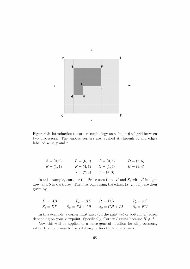
A B
C D
x
y
z
w
E F
JI
HG
Figure 6.3: Introduction to corner terminology on a simple 6×6 grid betweentwo processors. The various corners are labelled A through J, and edgeslabelled w, x, y and z.
A = (0, 0) B = (6, 0) C = (0, 6) D = (6, 6)
E = (1, 1) F = (4, 1) G = (1, 4) H = (2, 4)
I = (2, 3) J = (4, 3)
In this example, consider the Processors to be P and S, with P in lightgrey, and S in dark grey. The lines composing the edges, (x, y, z, w), are thengiven by,
Pz = AB Pw = BD Px = CD Py = AC
Sz = EF Sw = FJ + IH Sx = GH + IJ Sy = EG
In this example, a corner must exist (on the right (w) or bottom (x) edge,depending on your viewpoint. Specifically, Corner I exists because H 6= J .
Now this will be applied to a more general notation for all processors,rather than continue to use arbitrary letters to denote corners.
68
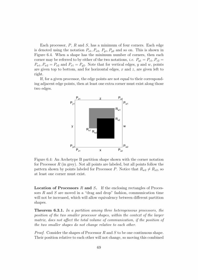
Each processor, P , R and S, has a minimum of four corners. Each edgeis denoted using the notation Px1, Px2, Py1, Py2 and so on. This is shown inFigure 6.4. When a shape has the minimum number of corners, then eachcorner may be referred to by either of the two notations, i.e. Py1 = Pz1, Pz2 =Pw1, Pw2 = Px2 and Px1 = Py2. Note that for vertical edges, y and w, pointsare given top to bottom, and for horizontal edges, x and z, are given left toright.
If, for a given processor, the edge points are not equal to their correspond-ing adjacent edge points, then at least one extra corner must exist along thosetwo edges.
y
x
z
w Rx1
Rx2
Rw2
Rw1
Px1 Px2
Py1
Py2
Pz1 Pz2 Pw1
Pw2
Figure 6.4: An Archetype B partition shape shown with the corner notationfor Processor R (in grey). Not all points are labeled, but all points follow thepattern shown by points labeled for Processor P . Notice that Rw2 6= Rx2, soat least one corner must exist.
Location of Processors R and S. If the enclosing rectangles of Proces-sors R and S are moved in a “drag and drop” fashion, communication timewill not be increased, which will allow equivalency between different partitionshapes.
Theorem 6.3.1. In a partition among three heterogeneous processors, theposition of the two smaller processor shapes, within the context of the largermatrix, does not affect the total volume of communication, if the position ofthe two smaller shapes do not change relative to each other.
Proof. Consider the shapes of Processor R and S to be one continuous shape.Their position relative to each other will not change, so moving this combined
69
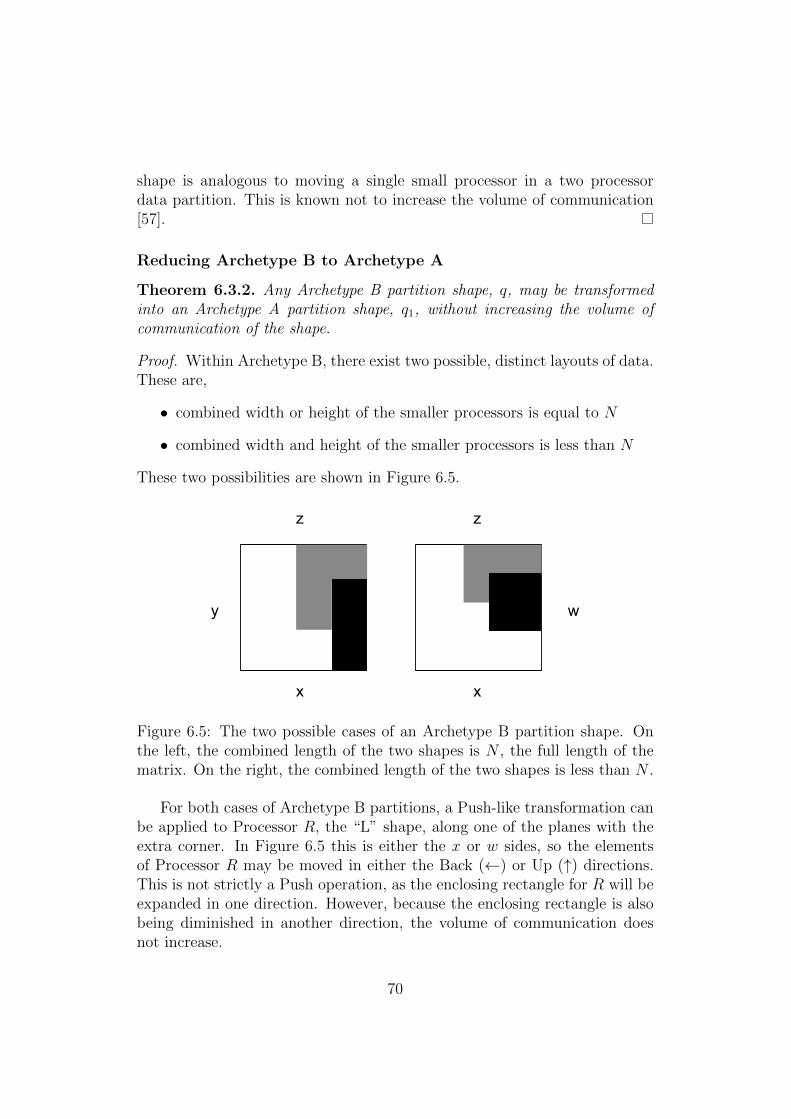
shape is analogous to moving a single small processor in a two processordata partition. This is known not to increase the volume of communication[57].
Reducing Archetype B to Archetype A
Theorem 6.3.2. Any Archetype B partition shape, q, may be transformedinto an Archetype A partition shape, q1, without increasing the volume ofcommunication of the shape.
Proof. Within Archetype B, there exist two possible, distinct layouts of data.These are,
• combined width or height of the smaller processors is equal to N
• combined width and height of the smaller processors is less than N
These two possibilities are shown in Figure 6.5.
x x
y w
z z
Figure 6.5: The two possible cases of an Archetype B partition shape. Onthe left, the combined length of the two shapes is N , the full length of thematrix. On the right, the combined length of the two shapes is less than N .
For both cases of Archetype B partitions, a Push-like transformation canbe applied to Processor R, the “L” shape, along one of the planes with theextra corner. In Figure 6.5 this is either the x or w sides, so the elementsof Processor R may be moved in either the Back (←) or Up (↑) directions.This is not strictly a Push operation, as the enclosing rectangle for R will beexpanded in one direction. However, because the enclosing rectangle is alsobeing diminished in another direction, the volume of communication doesnot increase.
70
In the first case, to move the elements of R, only one transformationdirection is available because the length N of the combined rectangles doesnot allow room for additional swaps. In the example of Figure 6.5 the onlyavailable direction is Back (←).
For each column transformed to remove elements of R, at most one col-umn previously not containing R will have elements of R introduced. Thisis assured, by definition, by virtue of the existence of the corner:
Rw1 → Rx2 < Ry1 → Ry2 (6.2)
where,
Rw1 → Rx2 = # of rows separating Rw1 and Rx2
Ry1 → Ry2 = # of rows separating Ry1 and Ry2
For the second case, the elements of R can be moved in either direction,as the combined length of both shapes is less than N , and therefore rowsand columns exist in either direction into which elements of R can be moved.The direction of the Push-like transformation is decided by choosing thatwhich requires the lower volume of elements to be moved. In example Figure6.5, first use Theorem 6.3.1 to move the entire shape of Processors R and Sdown in the matrix so that Sx2 = Px2, opening rows above Processor R soelements may be moved in the Up (↑) direction.
For each row transformed to remove elements of R, at most one rowpreviously not containing R will have elements of R introduced. This isassured by definition, by virtue of the existence of the corner:
Rx1 → Rw2 < Rz1 → Rz2 (6.3)
where,
Rx1 → Rw2 = # of rows separating Rx1 and Rw2
Rz1 → Rz2 = # of rows separating Rz1 and Rz2
For every row or column made dirty with R during these transformations,a row or column must have, by definition been made clean of R, so volumeof communication is constant or decreasing.
Archetype C to Archetype A
Theorem 6.3.3. Any Archetype C partition shape, q, may be transformedinto a Archetype A partition shape, q1, without increasing the volume of com-munication of the shape by applying the Push operation.
71
Proof. By definition of this shape, valid Push operations remain, which ifapplied will result in an Archetype A partition.
Archetype C is the only archetype formed by the DFA program on whichthere are valid Push operations remaining. These form as a result of therandomised Push direction algorithm, and is a necessary downside to trulyconsidering every possible partition shape without preconceived notions ofthe final shape. Transforming partition shapes of this archetype is a simplematter of applying the Push operation in the direction not selected by theprogram.
In the program, these cases are handled by a “beautify” function to returnrectangular or asymptotically rectangular shapes, however Archetype C isincluded here for comprehensiveness.
Archetype D to Archetype A
Theorem 6.3.4. Any Archetype D partition shape, q, may be transformedinto an Archetype A partition shape, q1, without increasing the volume ofcommunication of the shape
Proof. In [57] it was proven that for two processors, the location of the smallerprocessor within the context of the larger matrix, does not effect the totalvolume of communication.
Consider the surrounding processor, in figures Processor R, and the innerprocessor, Processor S, to be a two processor partition in a matrix the sizeof Processor R’s enclosing rectangle.
By [57] Theorem 3.4 Canonical Forms, move Processor S so that Rx2 =Sx2.
An Archetype B partition has now been created from an Archetype D,without increasing its volume of communication. By Theorem 6.3.2, it maybe further reduced to Archetype A.
6.4 Push Technique on Four or More Proces-
sors
The additional conditions introduced for Push on three processors are neces-sary and sufficient for using the Push Technique on four or more processors.Each inactive processor, including any arbitrarily large numbers of proces-sors, must not,
• have its enclosing rectangle enlarged
72
• make dirty a number of rows and columns, without cleaning an greateror equal amount of rows and columns
However, as the number of processors increases, so does the likelihoodthat some arbitrary shape will be found that cannot be improved upon bythe Push Technique. If the Push Technique were to regularly run into arbi-trary arrangements of elements which are not true candidates, but which aredead ends beyond which is cannot progress, would significantly hamper itsusefulness.
To accommodate this problem, a larger matrix size could be used to in-crease the granularity of the experimental runs. In this way, it is foreseeablethat the Push Technique can be experimentally expanded to six, eight, oreven ten abstract processors. And as an abstract processor can actually rep-resent myriad computing resources, if the Push Technique is used at varying,hierarchical levels, there should be no limit to the number of processors it canbe applied to. While this is outside the scope of this thesis, it does presentexciting possibilities which are discussed further in Chapter 10.
73
Chapter 7
Three Processor OptimalPartition Shape
The next step in using the Push Technique is to find the optimal data par-tition for three processors, building on the work done with two processors.The Push DFA provides motivation for this postulate:
Postulate 1 (Three Processor Push). There exists no arrangement of el-ements among three heterogeneous processors in an N × N matrix whichcannot be improved with the Push operation, except those arrangements ofshapes defined as Archetypes A, B, C, and D.
As it was shown in Chapter 4, the optimal shapes must lie within ArchetypeA, as all other Archetypes may be reduced to it without increasing commu-nication volume. This chapter will evaluate all the possible shapes withinthe Archetype A to determine the optimal partition shape for all compu-tational power ratios, four different network topologies, and the five matrixmultiplication algorithms.
7.1 Archetype A: Candidate Shapes
A wide variety of partition shapes exist within Archetype A. All of theseshapes may be further categorised into six partition shape types. The can-didate partition types included under Archetype A, found experimentally bythe Push DFA, are seen in Figure 7.1. In all six, Processors R and S are as-signed rectangular portions of the matrix to compute. These rectangles varyin length from, at the longest, N to, at the shortest,
√#X, i.e. the side of a
square containing all the elements of Processor X. Processor P is assigned arectangular portion in three of the shape types, and non-rectangular portionin the remaining three types.
74
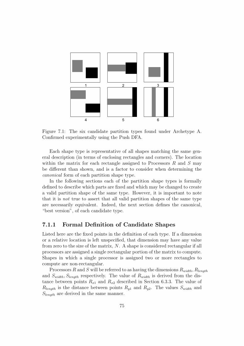
1 2 3
4 5 6
Figure 7.1: The six candidate partition types found under Archetype A.Confirmed experimentally using the Push DFA.
Each shape type is representative of all shapes matching the same gen-eral description (in terms of enclosing rectangles and corners). The locationwithin the matrix for each rectangle assigned to Processors R and S maybe different than shown, and is a factor to consider when determining thecanonical form of each partition shape type.
In the following sections each of the partition shape types is formallydefined to describe which parts are fixed and which may be changed to createa valid partition shape of the same type. However, it is important to notethat it is not true to assert that all valid partition shapes of the same typeare necessarily equivalent. Indeed, the next section defines the canonical,“best version”, of each candidate type.
7.1.1 Formal Definition of Candidate Shapes
Listed here are the fixed points in the definition of each type. If a dimensionor a relative location is left unspecified, that dimension may have any valuefrom zero to the size of the matrix, N . A shape is considered rectangular if allprocessors are assigned a single rectangular portion of the matrix to compute.Shapes in which a single processor is assigned two or more rectangles tocompute are non-rectangular.
ProcessorsR and S will be referred to as having the dimensionsRwidth, Rlength
and Swidth, Slength respectively. The value of Rwidth is derived from the dis-tance between points Rx1 and Rx2 described in Section 6.3.3. The value ofRlength is the distance between points Ry1 and Ry2. The values Swidth andSlength are derived in the same manner.
75
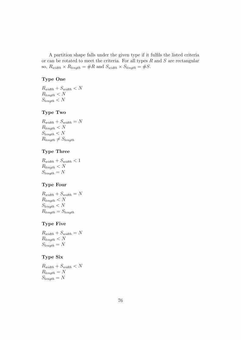
A partition shape falls under the given type if it fulfils the listed criteriaor can be rotated to meet the criteria. For all types R and S are rectangularso, Rwidth ×Rlength = #R and Swidth × Slength = #S.
Type One
Rwidth + Swidth < NRlength < NSlength < N
Type Two
Rwidth + Swidth = NRlength < NSlength < NRlength 6= Slength
Type Three
Rwidth + Swidth < 1Rlength < NSlength = N
Type Four
Rwidth + Swidth = NRlength < NSlength < NRlength = Slength
Type Five
Rwidth + Swidth = NRlength < NSlength = N
Type Six
Rwidth + Swidth < NRlength = NSlength = N
76
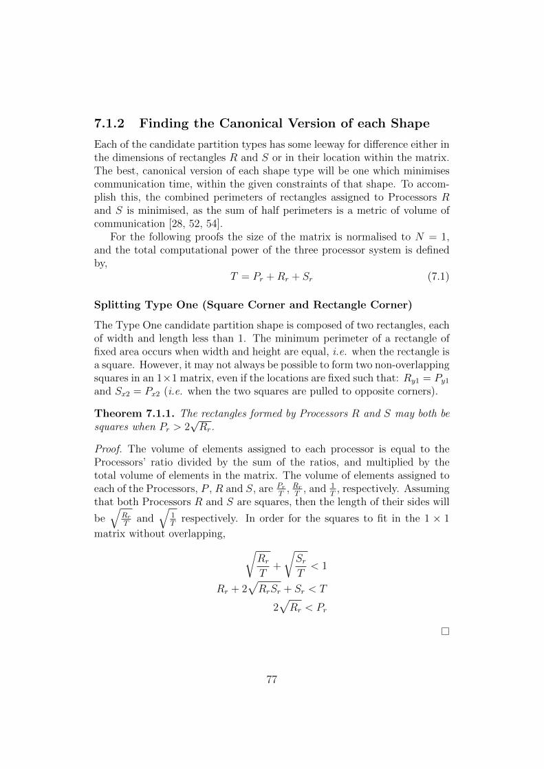
7.1.2 Finding the Canonical Version of each Shape
Each of the candidate partition types has some leeway for difference either inthe dimensions of rectangles R and S or in their location within the matrix.The best, canonical version of each shape type will be one which minimisescommunication time, within the given constraints of that shape. To accom-plish this, the combined perimeters of rectangles assigned to Processors Rand S is minimised, as the sum of half perimeters is a metric of volume ofcommunication [28, 52, 54].
For the following proofs the size of the matrix is normalised to N = 1,and the total computational power of the three processor system is definedby,
T = Pr +Rr + Sr (7.1)
Splitting Type One (Square Corner and Rectangle Corner)
The Type One candidate partition shape is composed of two rectangles, eachof width and length less than 1. The minimum perimeter of a rectangle offixed area occurs when width and height are equal, i.e. when the rectangle isa square. However, it may not always be possible to form two non-overlappingsquares in an 1×1 matrix, even if the locations are fixed such that: Ry1 = Py1and Sx2 = Px2 (i.e. when the two squares are pulled to opposite corners).
Theorem 7.1.1. The rectangles formed by Processors R and S may both besquares when Pr > 2
√Rr.
Proof. The volume of elements assigned to each processor is equal to theProcessors’ ratio divided by the sum of the ratios, and multiplied by thetotal volume of elements in the matrix. The volume of elements assigned toeach of the Processors, P , R and S, are Pr
T, Rr
T, and 1
T, respectively. Assuming
that both Processors R and S are squares, then the length of their sides will
be√
Rr
Tand
√1T
respectively. In order for the squares to fit in the 1 × 1
matrix without overlapping, √Rr
T+
√SrT< 1
Rr + 2√RrSr + Sr < T
2√Rr < Pr
77
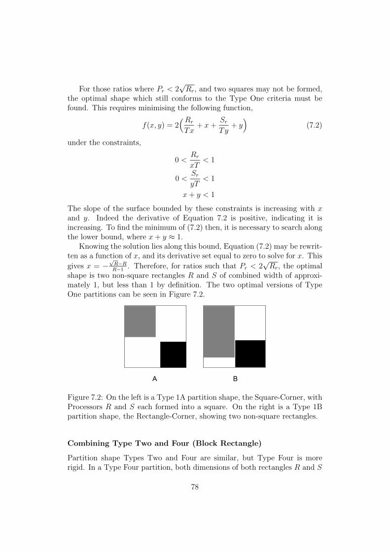
For those ratios where Pr < 2√Rr, and two squares may not be formed,
the optimal shape which still conforms to the Type One criteria must befound. This requires minimising the following function,
f(x, y) = 2(Rr
Tx+ x+
SrTy
+ y)
(7.2)
under the constraints,
0 <Rr
xT< 1
0 <SryT
< 1
x+ y < 1
The slope of the surface bounded by these constraints is increasing with xand y. Indeed the derivative of Equation 7.2 is positive, indicating it isincreasing. To find the minimum of (7.2) then, it is necessary to search alongthe lower bound, where x+ y ≈ 1.
Knowing the solution lies along this bound, Equation (7.2) may be rewrit-ten as a function of x, and its derivative set equal to zero to solve for x. This
gives x = −√R−RR−1 . Therefore, for ratios such that Pr < 2
√Rr, the optimal
shape is two non-square rectangles R and S of combined width of approxi-mately 1, but less than 1 by definition. The two optimal versions of TypeOne partitions can be seen in Figure 7.2.
A B
Figure 7.2: On the left is a Type 1A partition shape, the Square-Corner, withProcessors R and S each formed into a square. On the right is a Type 1Bpartition shape, the Rectangle-Corner, showing two non-square rectangles.
Combining Type Two and Four (Block Rectangle)
Partition shape Types Two and Four are similar, but Type Four is morerigid. In a Type Four partition, both dimensions of both rectangles R and S
78
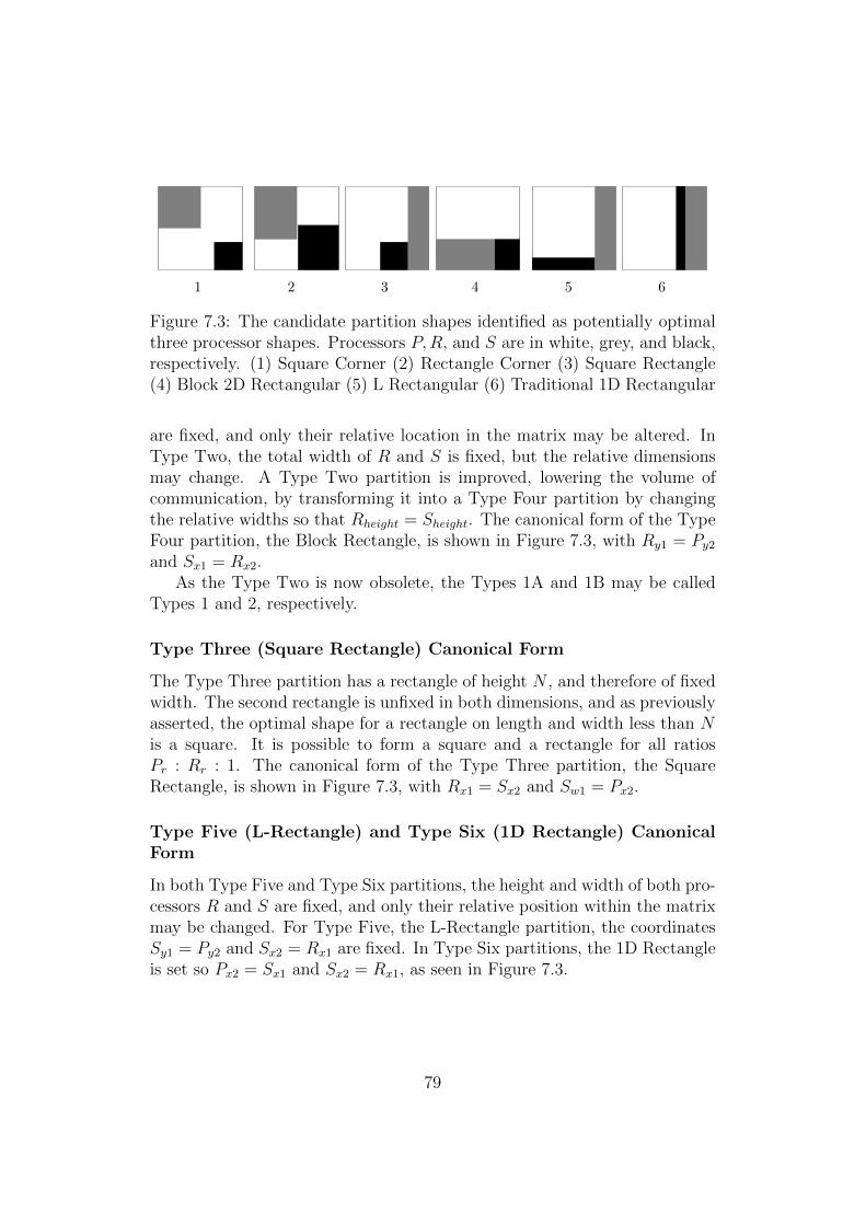
1 2 3 4 5 6
Figure 7.3: The candidate partition shapes identified as potentially optimalthree processor shapes. Processors P,R, and S are in white, grey, and black,respectively. (1) Square Corner (2) Rectangle Corner (3) Square Rectangle(4) Block 2D Rectangular (5) L Rectangular (6) Traditional 1D Rectangular
are fixed, and only their relative location in the matrix may be altered. InType Two, the total width of R and S is fixed, but the relative dimensionsmay change. A Type Two partition is improved, lowering the volume ofcommunication, by transforming it into a Type Four partition by changingthe relative widths so that Rheight = Sheight. The canonical form of the TypeFour partition, the Block Rectangle, is shown in Figure 7.3, with Ry1 = Py2and Sx1 = Rx2.
As the Type Two is now obsolete, the Types 1A and 1B may be calledTypes 1 and 2, respectively.
Type Three (Square Rectangle) Canonical Form
The Type Three partition has a rectangle of height N , and therefore of fixedwidth. The second rectangle is unfixed in both dimensions, and as previouslyasserted, the optimal shape for a rectangle on length and width less than Nis a square. It is possible to form a square and a rectangle for all ratiosPr : Rr : 1. The canonical form of the Type Three partition, the SquareRectangle, is shown in Figure 7.3, with Rx1 = Sx2 and Sw1 = Px2.
Type Five (L-Rectangle) and Type Six (1D Rectangle) CanonicalForm
In both Type Five and Type Six partitions, the height and width of both pro-cessors R and S are fixed, and only their relative position within the matrixmay be changed. For Type Five, the L-Rectangle partition, the coordinatesSy1 = Py2 and Sx2 = Rx1 are fixed. In Type Six partitions, the 1D Rectangleis set so Px2 = Sx1 and Sx2 = Rx1, as seen in Figure 7.3.
79
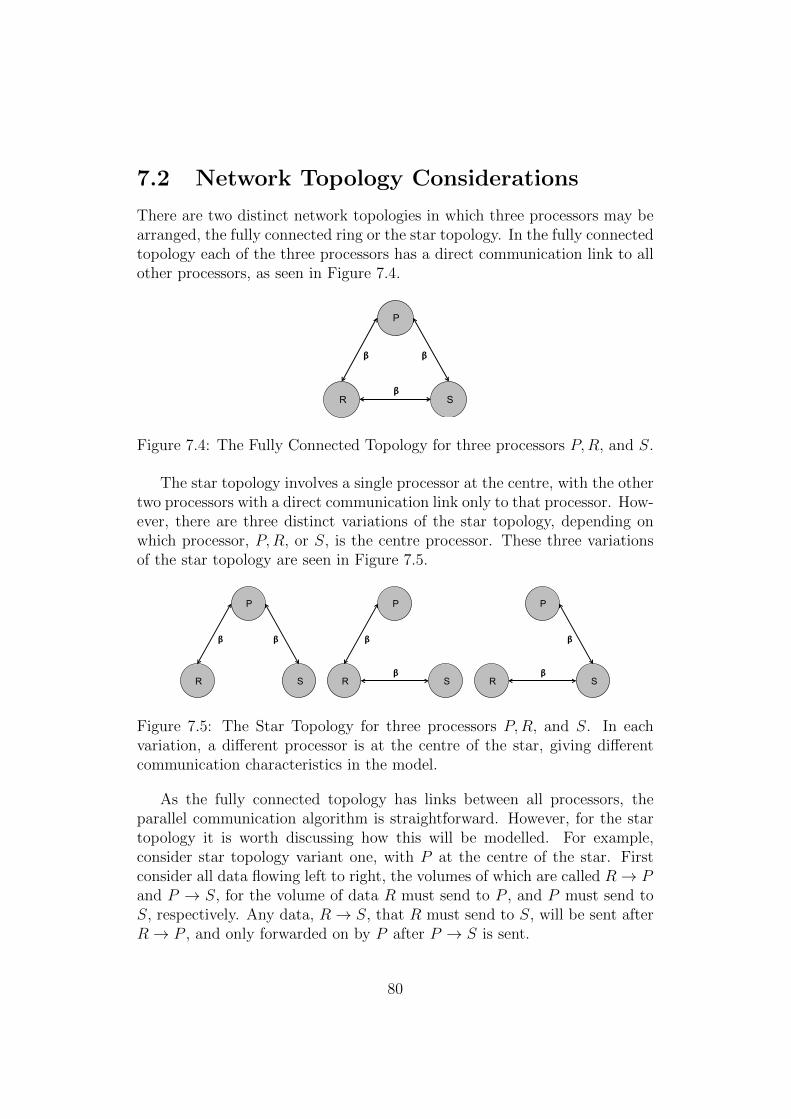
7.2 Network Topology Considerations
There are two distinct network topologies in which three processors may bearranged, the fully connected ring or the star topology. In the fully connectedtopology each of the three processors has a direct communication link to allother processors, as seen in Figure 7.4.
P
R S
β
β
β
Figure 7.4: The Fully Connected Topology for three processors P,R, and S.
The star topology involves a single processor at the centre, with the othertwo processors with a direct communication link only to that processor. How-ever, there are three distinct variations of the star topology, depending onwhich processor, P,R, or S, is the centre processor. These three variationsof the star topology are seen in Figure 7.5.
P
R S
β
β
P
R S
β β
P
R S β
β
Figure 7.5: The Star Topology for three processors P,R, and S. In eachvariation, a different processor is at the centre of the star, giving differentcommunication characteristics in the model.
As the fully connected topology has links between all processors, theparallel communication algorithm is straightforward. However, for the startopology it is worth discussing how this will be modelled. For example,consider star topology variant one, with P at the centre of the star. Firstconsider all data flowing left to right, the volumes of which are called R→ Pand P → S, for the volume of data R must send to P , and P must send toS, respectively. Any data, R→ S, that R must send to S, will be sent afterR→ P , and only forwarded on by P after P → S is sent.
80
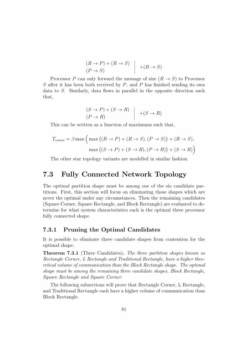
(R→ P ) + (R→ S)
(P → S)+(R→ S)
Processor P can only forward the message of size (R → S) to ProcessorS after it has been both received by P , and P has finished sending its owndata to S. Similarly, data flows in parallel in the opposite direction suchthat,
(S → P ) + (S → R)
(P → R)+(S → R)
This can be written as a function of maximums such that,
Tcomm = βmax(
max((R→ P ) + (R→ S), (P → S)
)+ (R→ S),
max((S → P ) + (S → R), (P → R)
)+ (S → R)
)The other star topology variants are modelled in similar fashion.
7.3 Fully Connected Network Topology
The optimal partition shape must be among one of the six candidate par-titions. First, this section will focus on eliminating those shapes which arenever the optimal under any circumstances. Then the remaining candidates(Square Corner, Square Rectangle, and Block Rectangle) are evaluated to de-termine for what system characteristics each is the optimal three processorfully connected shape.
7.3.1 Pruning the Optimal Candidates
It is possible to eliminate three candidate shapes from contention for theoptimal shape.
Theorem 7.3.1 (Three Candidates). The three partition shapes known asRectangle Corner, L Rectangle and Traditional Rectangle, have a higher theo-retical volume of communication than the Block Rectangle shape. The optimalshape must be among the remaining three candidate shapes, Block Rectangle,Square Rectangle and Square Corner.
The following subsections will prove that Rectangle Corner, L Rectangle,and Traditional Rectangle each have a higher volume of communication thanBlock Rectangle.
81
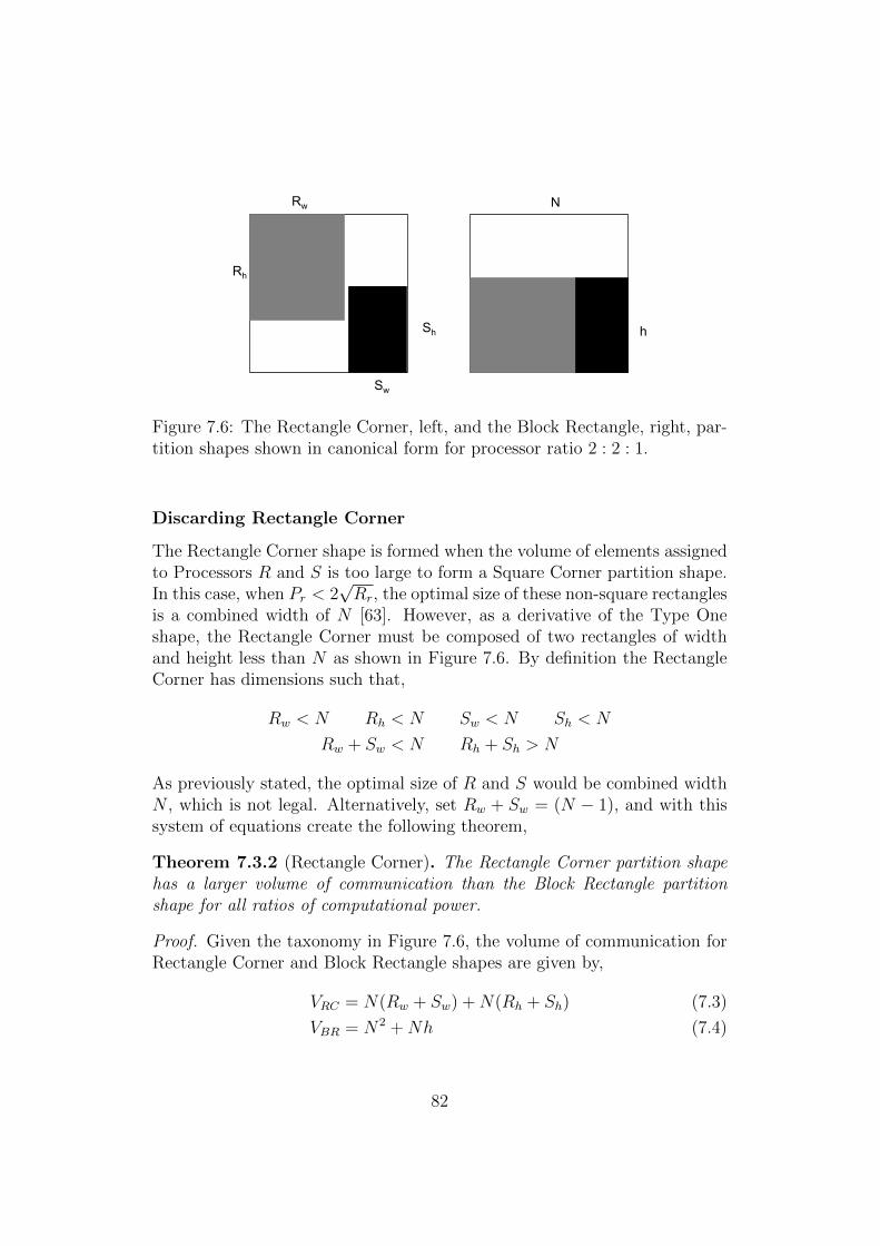
Rw
Rh
Sw
Sh h
N
Figure 7.6: The Rectangle Corner, left, and the Block Rectangle, right, par-tition shapes shown in canonical form for processor ratio 2 : 2 : 1.
Discarding Rectangle Corner
The Rectangle Corner shape is formed when the volume of elements assignedto Processors R and S is too large to form a Square Corner partition shape.In this case, when Pr < 2
√Rr, the optimal size of these non-square rectangles
is a combined width of N [63]. However, as a derivative of the Type Oneshape, the Rectangle Corner must be composed of two rectangles of widthand height less than N as shown in Figure 7.6. By definition the RectangleCorner has dimensions such that,
Rw < N Rh < N Sw < N Sh < N
Rw + Sw < N Rh + Sh > N
As previously stated, the optimal size of R and S would be combined widthN , which is not legal. Alternatively, set Rw + Sw = (N − 1), and with thissystem of equations create the following theorem,
Theorem 7.3.2 (Rectangle Corner). The Rectangle Corner partition shapehas a larger volume of communication than the Block Rectangle partitionshape for all ratios of computational power.
Proof. Given the taxonomy in Figure 7.6, the volume of communication forRectangle Corner and Block Rectangle shapes are given by,
VRC = N(Rw + Sw) +N(Rh + Sh) (7.3)
VBR = N2 +Nh (7.4)
82
N
Rw Sw
Sh
Figure 7.7: The canonical form of the L Rectangular partition shape withprocessor ratio 4 : 2 : 1.
Substitute Rw + Sw = (N − 1), and create the inequality given by,
BR < RC
N + h < N − 1 +Rh + Sh
h+ 1 < Rh + Sh
h ≤ Rh + Sh
By definition, Rh + Sh > N and h < N , so this is true.
Discarding L Rectangle
The L Rectangle partition shape, composed of an N height rectangle forProcessor R and a rectangle for Processor S such that the combined widthof S and R is N , can be seen in Figure 7.7. The width, Sw, of Processor Sis given in terms of the known fixed width of Processor R.
VLR = N2 +NSw (7.5)
Sw = N − RrN
T
Theorem 7.3.3 (L Rectangle). The L Rectangle partition shape has a vol-ume of communication larger than or equal to the Block Rectangle partitionshape for all processor ratios.
Proof. Note that h can be expressed as a function of the number of elementsassigned to Processor P such that, h = N − PrN
T. Begin by stating the
83
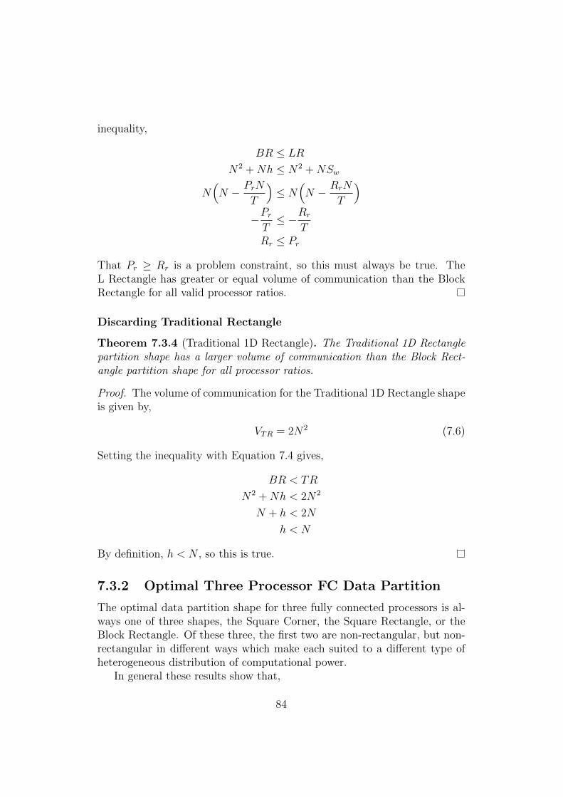
inequality,
BR ≤ LR
N2 +Nh ≤ N2 +NSw
N(N − PrN
T
)≤ N
(N − RrN
T
)−PrT≤ −Rr
TRr ≤ Pr
That Pr ≥ Rr is a problem constraint, so this must always be true. TheL Rectangle has greater or equal volume of communication than the BlockRectangle for all valid processor ratios.
Discarding Traditional Rectangle
Theorem 7.3.4 (Traditional 1D Rectangle). The Traditional 1D Rectanglepartition shape has a larger volume of communication than the Block Rect-angle partition shape for all processor ratios.
Proof. The volume of communication for the Traditional 1D Rectangle shapeis given by,
VTR = 2N2 (7.6)
Setting the inequality with Equation 7.4 gives,
BR < TR
N2 +Nh < 2N2
N + h < 2N
h < N
By definition, h < N , so this is true.
7.3.2 Optimal Three Processor FC Data Partition
The optimal data partition shape for three fully connected processors is al-ways one of three shapes, the Square Corner, the Square Rectangle, or theBlock Rectangle. Of these three, the first two are non-rectangular, but non-rectangular in different ways which make each suited to a different type ofheterogeneous distribution of computational power.
In general these results show that,
84
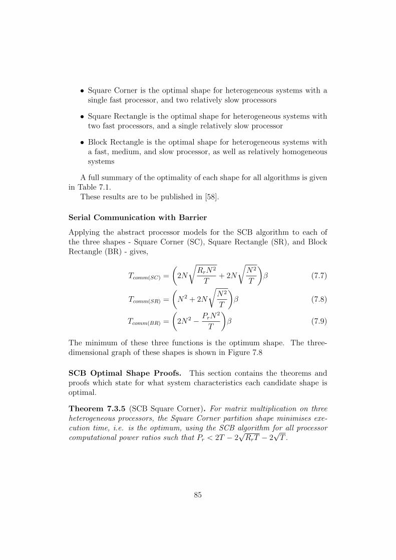
• Square Corner is the optimal shape for heterogeneous systems with asingle fast processor, and two relatively slow processors
• Square Rectangle is the optimal shape for heterogeneous systems withtwo fast processors, and a single relatively slow processor
• Block Rectangle is the optimal shape for heterogeneous systems witha fast, medium, and slow processor, as well as relatively homogeneoussystems
A full summary of the optimality of each shape for all algorithms is givenin Table 7.1.
These results are to be published in [58].
Serial Communication with Barrier
Applying the abstract processor models for the SCB algorithm to each ofthe three shapes - Square Corner (SC), Square Rectangle (SR), and BlockRectangle (BR) - gives,
Tcomm(SC) =
(2N
√RrN2
T+ 2N
√N2
T
)β (7.7)
Tcomm(SR) =
(N2 + 2N
√N2
T
)β (7.8)
Tcomm(BR) =
(2N2 − PrN
2
T
)β (7.9)
The minimum of these three functions is the optimum shape. The three-dimensional graph of these shapes is shown in Figure 7.8
SCB Optimal Shape Proofs. This section contains the theorems andproofs which state for what system characteristics each candidate shape isoptimal.
Theorem 7.3.5 (SCB Square Corner). For matrix multiplication on threeheterogeneous processors, the Square Corner partition shape minimises exe-cution time, i.e. is the optimum, using the SCB algorithm for all processorcomputational power ratios such that Pr < 2T − 2
√RrT − 2
√T .
85
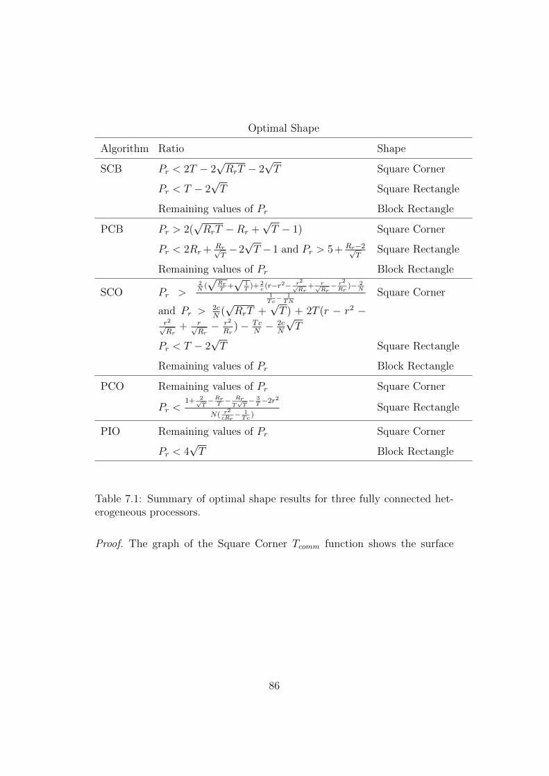
Optimal Shape
Algorithm Ratio Shape
SCB Pr < 2T − 2√RrT − 2
√T Square Corner
Pr < T − 2√T Square Rectangle
Remaining values of Pr Block Rectangle
PCB Pr > 2(√RrT −Rr +
√T − 1) Square Corner
Pr < 2Rr + Rr√T−2√T −1 and Pr > 5+ Rr−2√
TSquare Rectangle
Remaining values of Pr Block Rectangle
SCO Pr >2N(√
RrT
+√
1T)+ 2
c(r−r2− r2√
Rr+ r√
Rr− r2
Rr)− 2
N1Tc− 1
TN
and Pr >2cN
(√RrT +
√T ) + 2T (r − r2 −
r2√Rr
+ r√Rr− r2
Rr)− Tc
N− 2c
N
√T
Square Corner
Pr < T − 2√T Square Rectangle
Remaining values of Pr Block Rectangle
PCO Remaining values of Pr Square Corner
Pr <1+ 2√
T−Rr
T− Rr
T√T− 3
T−2r2
N( r2
cRr− 1
Tc)
Square Rectangle
PIO Remaining values of Pr Square Corner
Pr < 4√T Block Rectangle
Table 7.1: Summary of optimal shape results for three fully connected het-erogeneous processors.
Proof. The graph of the Square Corner Tcomm function shows the surface
86
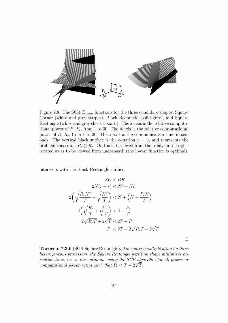
30
1
20 Pr Rr
Time (s)
Figure 7.8: The SCB Tcomm functions for the three candidate shapes, SquareCorner (white and grey stripes), Block Rectangle (solid grey), and SquareRectangle (white and grey checkerboard). The x-axis is the relative computa-tional power of P , Pr, from 1 to 30. The y-axis is the relative computationalpower of R, Rr, from 1 to 20. The z-axis is the communication time in sec-onds. The vertical black surface is the equation x = y, and represents theproblem constraint Pr ≥ Rr. On the left, viewed from the front, on the right,rotated so as to be viewed from underneath (the lowest function is optimal).
intersects with the Block Rectangle surface.
SC < BR
2N(r + s) < N2 +Nh
2
(√RrN2
T+
√N2
T
)< N +
(N − PrN
T
)2
(√Rr
T+
√1
T
)< 2− Pr
T
2√RrT + 2
√T < 2T − PrPr < 2T − 2
√RrT − 2
√T
Theorem 7.3.6 (SCB Square Rectangle). For matrix multiplication on threeheterogeneous processors, the Square Rectangle partition shape minimises ex-ecution time, i.e. is the optimum, using the SCB algorithm for all processorcomputational power ratios such that Pr < T − 2
√T .
87
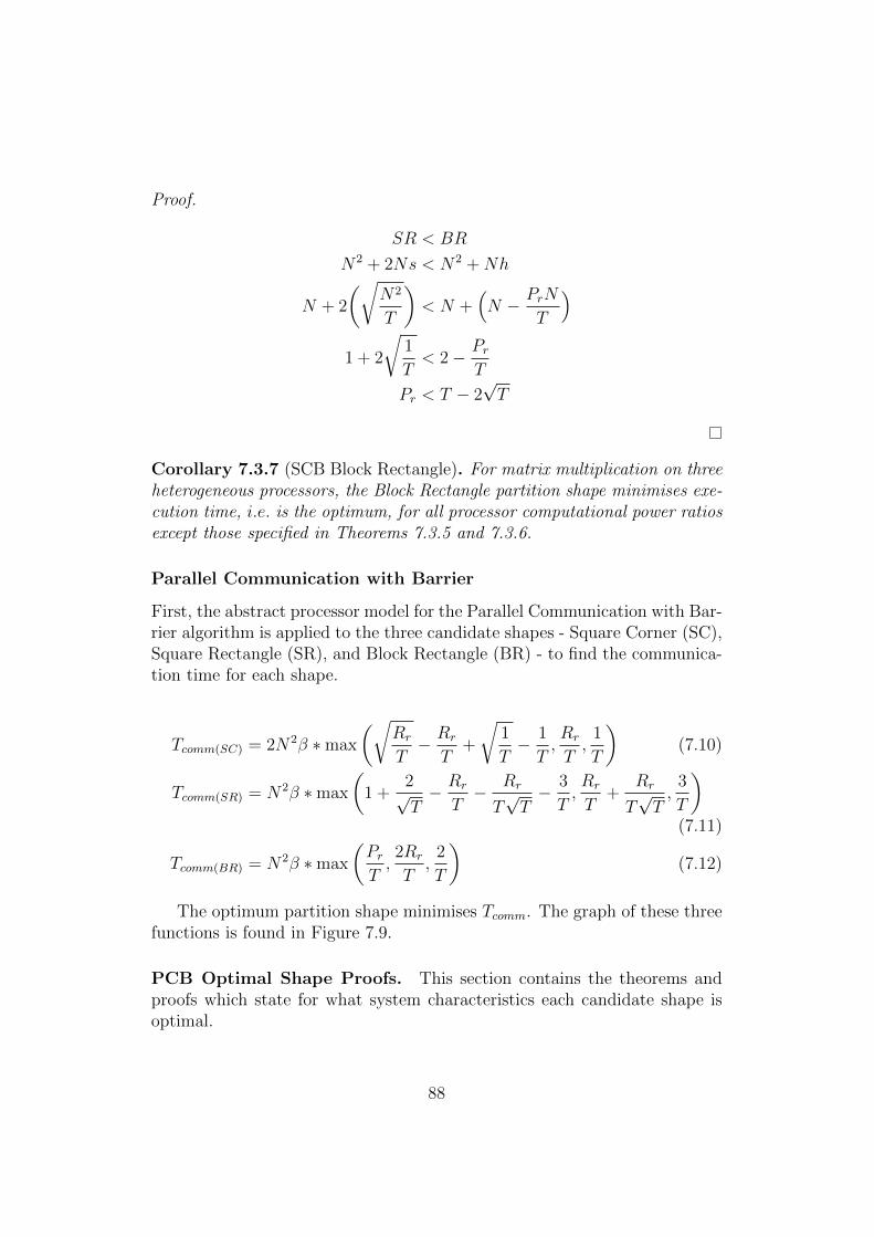
Proof.
SR < BR
N2 + 2Ns < N2 +Nh
N + 2
(√N2
T
)< N +
(N − PrN
T
)1 + 2
√1
T< 2− Pr
T
Pr < T − 2√T
Corollary 7.3.7 (SCB Block Rectangle). For matrix multiplication on threeheterogeneous processors, the Block Rectangle partition shape minimises exe-cution time, i.e. is the optimum, for all processor computational power ratiosexcept those specified in Theorems 7.3.5 and 7.3.6.
Parallel Communication with Barrier
First, the abstract processor model for the Parallel Communication with Bar-rier algorithm is applied to the three candidate shapes - Square Corner (SC),Square Rectangle (SR), and Block Rectangle (BR) - to find the communica-tion time for each shape.
Tcomm(SC) = 2N2β ∗max
(√Rr
T− Rr
T+
√1
T− 1
T,Rr
T,
1
T
)(7.10)
Tcomm(SR) = N2β ∗max
(1 +
2√T− Rr
T− Rr
T√T− 3
T,Rr
T+
Rr
T√T,
3
T
)(7.11)
Tcomm(BR) = N2β ∗max
(PrT,2Rr
T,
2
T
)(7.12)
The optimum partition shape minimises Tcomm. The graph of these threefunctions is found in Figure 7.9.
PCB Optimal Shape Proofs. This section contains the theorems andproofs which state for what system characteristics each candidate shape isoptimal.
88
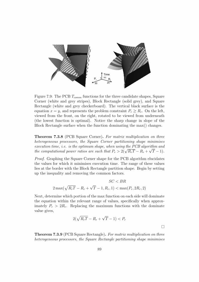
30
1
20 Pr Rr
Time (s)
Figure 7.9: The PCB Tcomm functions for the three candidate shapes, SquareCorner (white and grey stripes), Block Rectangle (solid grey), and SquareRectangle (white and grey checkerboard). The vertical black surface is theequation x = y, and represents the problem constraint Pr ≥ Rr. On the left,viewed from the front, on the right, rotated to be viewed from underneath(the lowest function is optimal). Notice the sharp change in slope of theBlock Rectangle surface when the function dominating the max() changes.
Theorem 7.3.8 (PCB Square Corner). For matrix multiplication on threeheterogeneous processors, the Square Corner partitioning shape minimisesexecution time, i.e. is the optimum shape, when using the PCB algorithm andthe computational power ratios are such that Pr > 2(
√RrT −Rr +
√T − 1).
Proof. Graphing the Square Corner shape for the PCB algorithm elucidatesthe values for which it minimises execution time. The range of these valueslies at the border with the Block Rectangle partition shape. Begin by settingup the inequality and removing the common factors.
SC < BR
2 max(√RrT −Rr +
√T − 1, Rr, 1) < max(Pr, 2Rr, 2)
Next, determine which portion of the max function on each side will dominatethe equation within the relevant range of values, specifically when approx-imately Pr > 2Rr. Replacing the maximum functions with the dominatevalue gives,
2(√RrT −Rr +
√T − 1) < Pr
Theorem 7.3.9 (PCB Square Rectangle). For matrix multiplication on threeheterogeneous processors, the Square Rectangle partitioning shape minimises
89
execution time, i.e. is the optimum shape, when using the PCB algorithmand the computational power ratios are such that Pr < 2Rr + Rr√
T− 2√T − 1
and Pr > 5 + Rr−2√T
.
Proof. Begin by stating the inequality and removing the common factors.
SR < BR
max(T + 2
√T −Rr −
Rr√T− 3, Rr +
Rr√T, 3)< max(Pr, 2Rr, 2)
It is clear from the graph that the problem space of 2Rr > Pr should be ex-amined more closely, to determine which functions dominate the maximumfunction for Square Rectangle and Block Rectangle for these ratios. Examin-ing SR, the graphs show that Pr > 5+ Rr−2√
Tmust be true before the first term
of the max function dominates the third term and the optimality inequalitybecomes,
T + 2√T −Rr −
Rr√T− 3 < 2Rr
Pr +Rr + 1 + 2√T −Rr −
Rr√T− 3 < 2Rr
Pr < 2Rr +Rr√T− 2√T − 1
Corollary 7.3.10 (PCB Block Rectangle). For matrix multiplication onthree heterogeneous processors, the Block Rectangle partition shape minimisesexecution time, i.e. is the optimum, for all processor computational powerratios except those specified in Theorems 7.3.8 and 7.3.9.
Serial Communication with Overlap
The Square Corner shape is the only partition shape which has an areawhich can be computed without communication. For the Square Rectangleand Block Rectangle shapes, the SCO algorithm is identical to the SerialCommunication with Barrier algorithm.
As with the two processor case for the Square Corner with the SCOalgorithm, it is necessary not only to apply the abstract processor model,but to determine the optimal volume of data to assign to Processors R andS. As the faster processor, Processor P , has a “jumpstart” on computation,it should be assigned a larger portion of the matrix in order to optimally
90
distribute the computational load. The optimal size of the square assignedto R (with the size assigned to S being in proportion) is,
r =2 + 2√
Rr
Pr
Rr+ 2√
Rr+ 2
Rr+ 2
(7.13)
And for those ratios of computational power at which the Square Cornerexecution time intersects with the execution times of Square Rectangle andBlock Rectangle (as seen in Figure 7.10), the execution time is given by,
Texe(SC)
N3β=
2
N
(√Rr
T+
√1
T
)+
2
c
(r − r2 − r2√
Rr
+r√Rr
− r2
Rr
)(7.14)
More information on the derivation of these results may be found in AppendixD.
Applying the abstract processor model to Square Rectangle and BlockRectangle gives the execution times as,
Texe(SR)
N3β=
1
N+
2
N
√1
T+ max
(PrTc,PrTc,PrTc
)Texe(BR)
N3β=
2
N− PrTN
+ max
(PrTc,PrTc,PrTc
)As with the two processor overlap algorithms, the constant factor of N3β
has been removed to facilitate the analysis of these equations.
SCO Optimal Shape Theorems. The proofs of the included theoremscan be found in Appendix D.
Theorem 7.3.11 (SCO Square Corner). For matrix multiplication on threeheterogeneous processors, the Square Corner partition shape minimises ex-ecution time, i.e. is the optimum shape, when using the SCO algorithm
for computational ratios such that Pr >2N(√
RrT
+√
1T)+ 2
c(r−r2− r2√
Rr+ r√
Rr− r2
Rr)− 2
N1Tc− 1
TN
and Pr >2cN
(√RrT +
√T )+2T (r− r2− r2√
Rr+ r√
Rr− r2
Rr)− Tc
N− 2c
N
√T , where
r is the optimal size of the square R, given in (7.13).
Theorem 7.3.12 (SCO Square Rectangle). For matrix multiplication onthree heterogeneous processors, the Square Rectangle partition shape min-imises execution time, i.e. is the optimum shape, when using the SCOalgorithm for computational ratios such that Pr < T − 2
√T and Pr <
2cN
(√RrT +
√T ) + 2T (r − r2 − r2√
Rr+ r√
Rr− r2
Rr)− Tc
N− 2c
N
√T
91
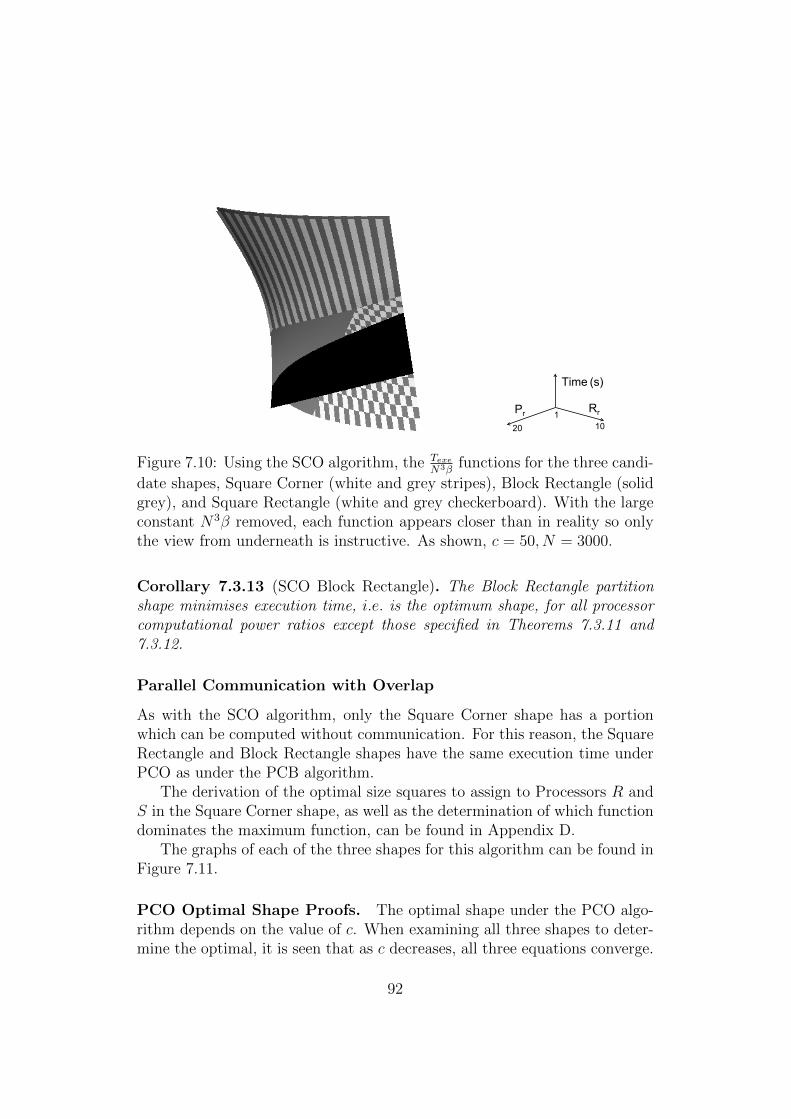
20 1
10
Pr Rr
Time (s)
Figure 7.10: Using the SCO algorithm, the TexeN3β
functions for the three candi-
date shapes, Square Corner (white and grey stripes), Block Rectangle (solidgrey), and Square Rectangle (white and grey checkerboard). With the largeconstant N3β removed, each function appears closer than in reality so onlythe view from underneath is instructive. As shown, c = 50, N = 3000.
Corollary 7.3.13 (SCO Block Rectangle). The Block Rectangle partitionshape minimises execution time, i.e. is the optimum shape, for all processorcomputational power ratios except those specified in Theorems 7.3.11 and7.3.12.
Parallel Communication with Overlap
As with the SCO algorithm, only the Square Corner shape has a portionwhich can be computed without communication. For this reason, the SquareRectangle and Block Rectangle shapes have the same execution time underPCO as under the PCB algorithm.
The derivation of the optimal size squares to assign to Processors R andS in the Square Corner shape, as well as the determination of which functiondominates the maximum function, can be found in Appendix D.
The graphs of each of the three shapes for this algorithm can be found inFigure 7.11.
PCO Optimal Shape Proofs. The optimal shape under the PCO algo-rithm depends on the value of c. When examining all three shapes to deter-mine the optimal, it is seen that as c decreases, all three equations converge.
92
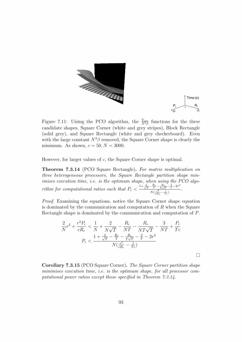
20 1
10
Pr Rr
Time (s)
Figure 7.11: Uising the PCO algorithm, the TexeN3β
functions for the three
candidate shapes, Square Corner (white and grey stripes), Block Rectangle(solid grey), and Square Rectangle (white and grey checkerboard). Evenwith the large constant N3β removed, the Square Corner shape is clearly theminimum. As shown, c = 50, N = 3000.
However, for larger values of c, the Square Corner shape is optimal.
Theorem 7.3.14 (PCO Square Rectangle). For matrix multiplication onthree heterogeneous processors, the Square Rectangle partition shape min-imises execution time, i.e. is the optimum shape, when using the PCO algo-
rithm for computational ratios such that Pr <1+ 2√
T−Rr
T− Rr
T√T− 3
T−2r2
N( r2
cRr− 1
Tc)
.
Proof. Examining the equations, notice the Square Corner shape equationis dominated by the communication and computation of R when the SquareRectangle shape is dominated by the communication and computation of P .
2
Nr2 +
r2PrcRr
<1
N+
2
N√T− Rr
NT− Rr
NT√T− 3
NT+PrTc
Pr <1 + 2√
T− Rr
T− Rr
T√T− 3
T− 2r2
N( r2
cRr− 1
Tc)
Corollary 7.3.15 (PCO Square Corner). The Square Corner partition shapeminimises execution time, i.e. is the optimum shape, for all processor com-putational power ratios except those specified in Theorem 7.3.14.
93
Parallel Interleaving Overlap
The Parallel Interleaving Overlap (PIO) algorithm, unlike the previous al-gorithms described, does not use bulk communication. At each step data issent, a row and a column (or k rows and columns) at a time, by the relevantprocessor(s) to all processor(s) requiring those elements, while, in parallel,all processors compute using the data sent in the previous step.
In the case of the PIO algorithm, the processors compute at the sametime, meaning the optimal distribution will be in proportion to their com-putational power. The optimal size of the r and s for the Square Corner is
therefore√
RrN2
Tand
√N2
T, respectively. In order to analyse the equations,
the constant factor N4β is removed and the focus placed on the dominantmiddle term which is multiplied by (N − 1).
Texe(SC)
N4β= max
(2
N2
(√Rr
T+
√1
T
),PrTc
)(7.15)
Texe(SR)
N4β= max
(2
N2
(1 + 2
√1
T
),PrTc
)(7.16)
Texe(BR)
N4β= max
(PrN2T
,PrTc
)(7.17)
PIO Optimal Shape Proofs.
Theorem 7.3.16 (PIO Block Rectangle). For matrix multiplication on threeheterogeneous processors, the Block Rectangle partition shape minimises ex-ecution time when using the PIO algorithm for computational power ratiossuch that Pr < 4
√T .
Proof. Either communication or computation will dominate the maximumfunction of all the potentially optimal partition shapes. If computation dom-inates, all shapes are equivalent. The communication will dominate the BlockRectangle partition shape when c > N2. In this case, the inequalities may
94
be set as follows.
BR < SC
PrN2T
<2
N2
(√Rr
T+
√1
T
)Pr < 2
√RrT + 2
√T
Pr < 4√T
BR < SR
PrN2T
<2
N2
(1 + 2
√1
T
)Pr < 2T + 2
√T Always true as by definition Pr < T
Corollary 7.3.17 (PIO Square Corner). The Square Corner partition shapeminimises execution time, i.e. is the optimum shape, for all processor com-putational power ratios except those specified in Theorem 7.3.16 when usingthe PIO algorithm.
7.3.3 Experimental Results
To validate the theoretical results of this paper experiments were undertakenon Grid’5000 in France using the Edel cluster at the Grenoble site. Each algo-rithm was tested using three nodes, comprised of 2 Intel Xeon E5520 2.2 GHzCPUs per node, with 4 cores per CPU. The communication interconnect isMPI over gigabit ethernet, and the computations use ATLAS. Heterogeneityin processing power was achieved using the cpulimit [62] program, an opensource code that limits the number of cycles a process may be active on theCPU to a percentage of the total.
Serial Communication with Barrier
The experimental results, for communication time, with the SCB algorithmcan be found in Figure 7.12. Note it is not possible to form a Square Cornershape at ratio 1 : 1 : 1. These experiments show that the theoretical optimumdoes indeed outperform the other possible shapes, which also perform inthe expected order. We did find, that while the Square Corner and Square
95
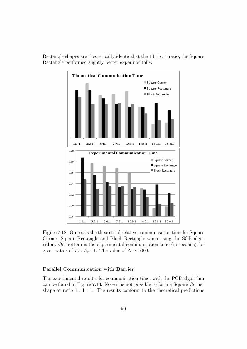
Rectangle shapes are theoretically identical at the 14 : 5 : 1 ratio, the SquareRectangle performed slightly better experimentally.
1:1:1 3:2:1 5:4:1 7:7:1 10:9:1 14:5:1 12:1:1 25:4:1
Theoretical Communication Time Square Corner
Square Rectangle
Block Rectangle
0.08
0.10
0.12
0.14
0.16
0.18
0.20
1:1:1 3:2:1 5:4:1 7:7:1 10:9:1 14:5:1 12:1:1 25:4:1
Experimental Communication Time
Square Corner Square Rectangle Block Rectangle
Figure 7.12: On top is the theoretical relative communication time for SquareCorner, Square Rectangle and Block Rectangle when using the SCB algo-rithm. On bottom is the experimental communication time (in seconds) forgiven ratios of Pr : Rr : 1. The value of N is 5000.
Parallel Communication with Barrier
The experimental results, for communication time, with the PCB algorithmcan be found in Figure 7.13. Note it is not possible to form a Square Cornershape at ratio 1 : 1 : 1. The results conform to the theoretical predictions
96
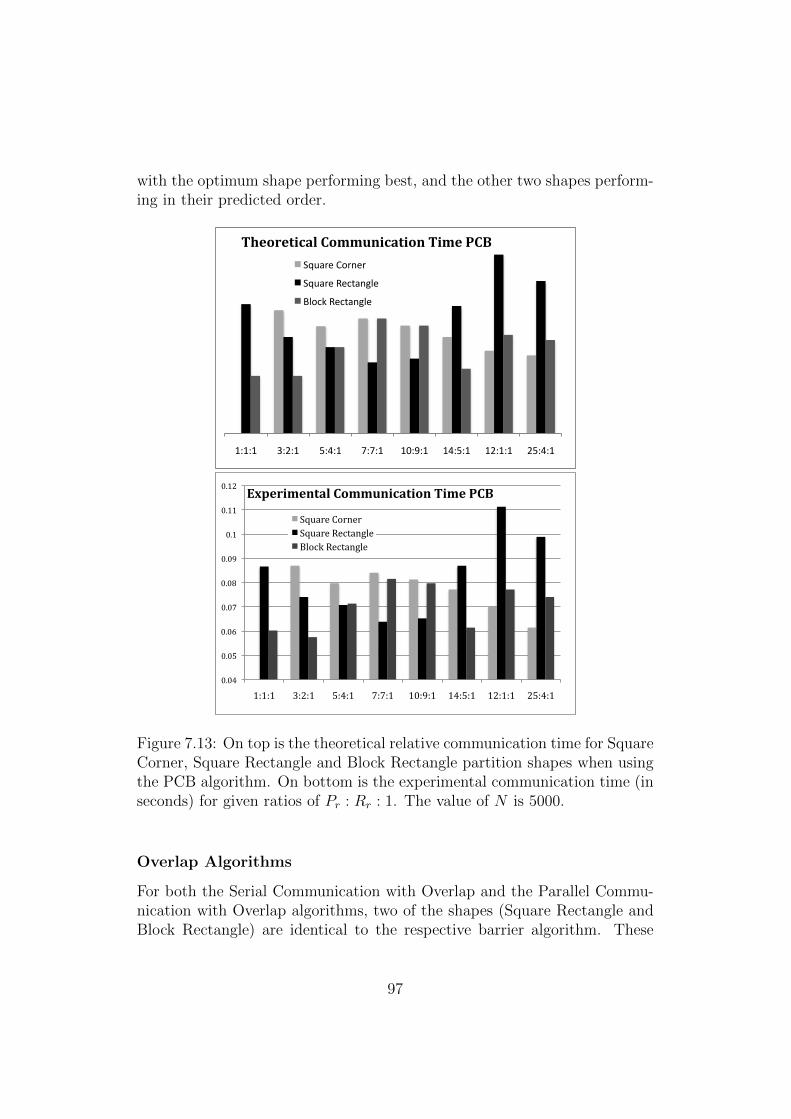
with the optimum shape performing best, and the other two shapes perform-ing in their predicted order.
1:1:1 3:2:1 5:4:1 7:7:1 10:9:1 14:5:1 12:1:1 25:4:1
Theoretical Communication Time PCB
Square Corner
Square Rectangle
Block Rectangle
0.04
0.05
0.06
0.07
0.08
0.09
0.1
0.11
0.12
1:1:1 3:2:1 5:4:1 7:7:1 10:9:1 14:5:1 12:1:1 25:4:1
Experimental Communication Time PCB
Square Corner Square Rectangle Block Rectangle
Figure 7.13: On top is the theoretical relative communication time for SquareCorner, Square Rectangle and Block Rectangle partition shapes when usingthe PCB algorithm. On bottom is the experimental communication time (inseconds) for given ratios of Pr : Rr : 1. The value of N is 5000.
Overlap Algorithms
For both the Serial Communication with Overlap and the Parallel Commu-nication with Overlap algorithms, two of the shapes (Square Rectangle andBlock Rectangle) are identical to the respective barrier algorithm. These
97
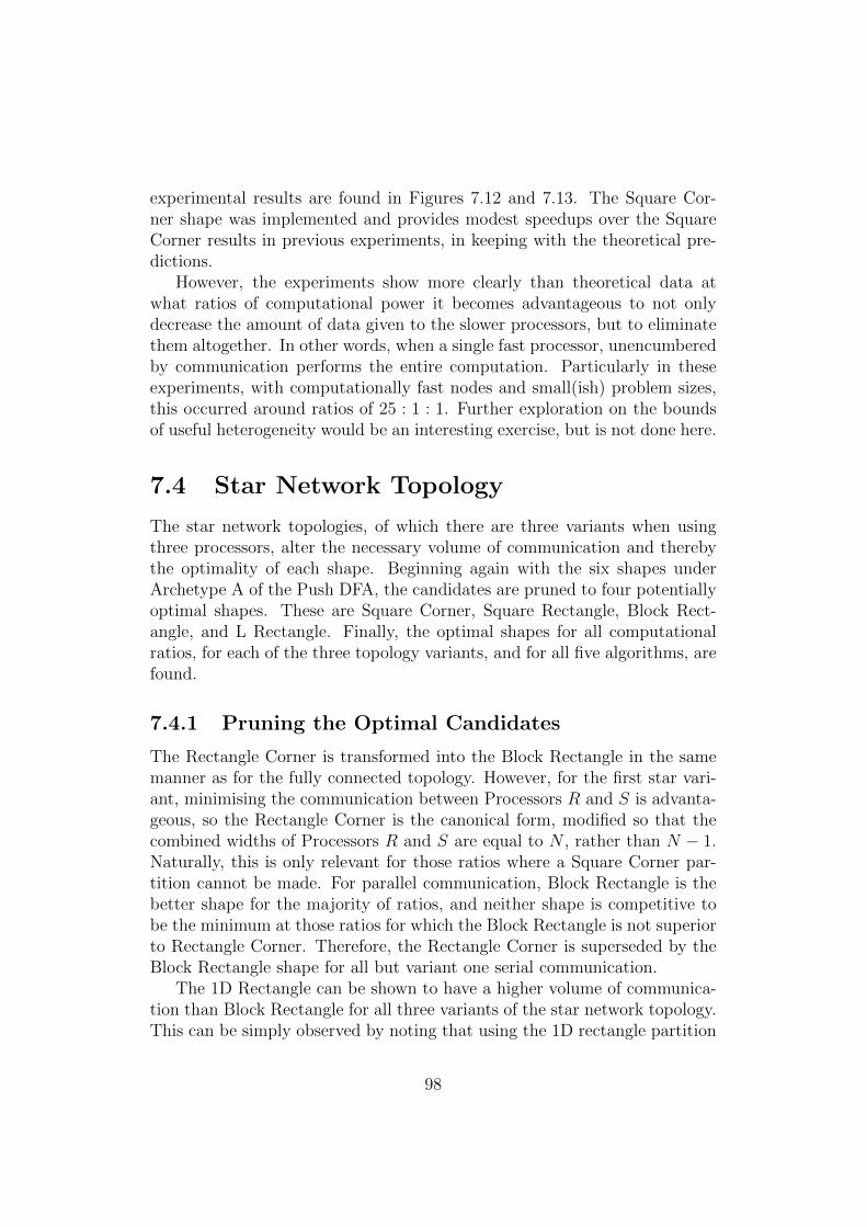
experimental results are found in Figures 7.12 and 7.13. The Square Cor-ner shape was implemented and provides modest speedups over the SquareCorner results in previous experiments, in keeping with the theoretical pre-dictions.
However, the experiments show more clearly than theoretical data atwhat ratios of computational power it becomes advantageous to not onlydecrease the amount of data given to the slower processors, but to eliminatethem altogether. In other words, when a single fast processor, unencumberedby communication performs the entire computation. Particularly in theseexperiments, with computationally fast nodes and small(ish) problem sizes,this occurred around ratios of 25 : 1 : 1. Further exploration on the boundsof useful heterogeneity would be an interesting exercise, but is not done here.
7.4 Star Network Topology
The star network topologies, of which there are three variants when usingthree processors, alter the necessary volume of communication and therebythe optimality of each shape. Beginning again with the six shapes underArchetype A of the Push DFA, the candidates are pruned to four potentiallyoptimal shapes. These are Square Corner, Square Rectangle, Block Rect-angle, and L Rectangle. Finally, the optimal shapes for all computationalratios, for each of the three topology variants, and for all five algorithms, arefound.
7.4.1 Pruning the Optimal Candidates
The Rectangle Corner is transformed into the Block Rectangle in the samemanner as for the fully connected topology. However, for the first star vari-ant, minimising the communication between Processors R and S is advanta-geous, so the Rectangle Corner is the canonical form, modified so that thecombined widths of Processors R and S are equal to N , rather than N − 1.Naturally, this is only relevant for those ratios where a Square Corner par-tition cannot be made. For parallel communication, Block Rectangle is thebetter shape for the majority of ratios, and neither shape is competitive tobe the minimum at those ratios for which the Block Rectangle is not superiorto Rectangle Corner. Therefore, the Rectangle Corner is superseded by theBlock Rectangle shape for all but variant one serial communication.
The 1D Rectangle can be shown to have a higher volume of communica-tion than Block Rectangle for all three variants of the star network topology.This can be simply observed by noting that using the 1D rectangle partition
98
shape requires each processor to send its entire volume of data to each otherprocessor. However, in the Block Rectangle, while Processors R and S dosend their entire volume to all processors, Processor P must only send aportion of it’s data to each other processor.
Therefore, the four candidate partition shapes to consider are SquareCorner, Square Rectangle, Block Rectangle (Rectangle Corner for variantone serial), and L Rectangle.
7.4.2 Applying the Abstract Processor Model
To apply the abstract processor model for each algorithm, first the necessaryvolume of data in each direction must be quantified for all four shapes.
r
r
s
s
a) Square Corner
N
s
s
Rw
b) Square Rectangle
h
Rw Sw
c-i) Block Rectangle
h
Rw
Sw
h
c-ii) Rectangle Corner
N
Sh Rw Sw
d) L Rectangle
Figure 7.14: The four candidate shapes for three heterogeneous processorswith a star network topology. The Block Rectangle canonical form is changedto Rectangle Corner for the first variant of the star topology only. Thelabels to the various dimensions allow the data volumes to be quantified forapplication of the abstract processor and algorithm models.
99
Volume of Communication
The total volume of communication, broken down by processor and directionis given for each candidate shape. However, note that while common namingconventions between shapes does not imply equal values, i.e. while Sw standsfor the width of Processor S in multiple shapes, the actual width of S in thoseshapes is not necessarily equivalent. Also note that if the entire volumeassigned to a given processor must be sent, it is given in the form of the ratiomultiplied by the number of elements in the matrix, e.g. PrN2
Tfor Processor
P .
Square Corner Volume of Communication. The Square Corner vol-ume of communication is derived using the naming scheme found in Figure7.14a. Processors R and S do not share any rows or columns, and thereforedo not need to communicate.
• P → R has data volume of 2r(N − r) elements
• P → S has data volume of 2s(N − s) elements
• R→ P has data volume of 2r2 elements
• R→ S has data volume of 0 elements, no communication necessary
• S → P has data volume of 2s2 elements
• S → R has data volume of 0 elements, no communication necessary
Square Rectangle Volume of Communication. The Square Rectanglevolume of communication is derived from Figure 7.14b.
• P → R has data volume of PrN2
Telements
• P → S has data volume of 2sN − 2s2 − sRw elements
• R→ P has data volume of RrN2
Telements
• R→ S has data volume of sRw elements
• S → P has data volume of 2s2 elements
• S → R has data volume of s2 elements
100
Block Rectangle Volume of Communication. The Block Rectanglevolume of communication is derived from Figure 7.14c-i. This is the canonicalshape for star topology variants two and three (when Processor R and S arethe centre of the star, respectively). It is also the canonical form for variantone type with parallel communication.
• P → R has data volume of Rw(N − h) elements
• P → S has data volume of Sw(N − h) elements
• R→ P has data volume of RrN2
Telements
• R→ S has data volume of RrN2
Telements
• S → P has data volume of N2
Telements
• S → R has data volume of N2
Telements
Rectangle Corner Volume of Communication. The Rectangle Cornervolume of communication is derived from Figure 7.14c-ii. This is the canoni-cal shape for star topology variant one, when Processor P is the centre of thestar, for serial communication. This decreases the communication betweenProcessors R and S, which is advantageous as no direct communication linkexists between these processors for this variant. For parallel communica-tion, there is a point at which the Block Rectangle is the better form, andRectangle Corner is never the minimum due to better performance by othershapes.
• P → R has data volume of PrN2
Telements
• P → S has data volume of PrN2
Telements
• R→ P has data volume of RrN2
T+Rw(N − h) elements
• R→ S has data volume of Rw(2h−N) elements
• S → P has data volume of N2
T+ Sw(N − h) elements
• S → R has data volume of Sw(2h−N) elements
101
L Rectangle Volume of Communication.
• P → R has data volume of PrN2
Telements
• P → S has data volume of PrN2
Telements
• R→ P has data volume of Rw(N − Sh) elements
• R→ S has data volume of RwSh elements
• S → P has data volume of N2
Telements
• S → R has data volume of N2
Telements
Model Equations by Shape, Variant, and Communication Algo-rithm
For each of the three variants of the star network topology, depicted in Figure7.5, the above communication volumes are translated into equations for bothserial and parallel communication. Note, in some places the equations havebeen simplified to increase readability. Particularly in the case of maximumfunctions, any terms which may be mathematically shown to never dominatethe maximum have been removed.
Variant One. The first variant of the star network topology puts ProcessorP at the centre of the star. Communication cost between Processor R andS is doubled, which is the worst case scenario.
The Variant One Serial Communication equations, for Square Corner,Square Rectangle, Rectangle Corner, and L Rectangle, are given respectivelyby,
Tcomm(SC)
N2= 2
√Rr
T+ 2
√1
T(7.18)
Tcomm(SR)
N2= 1 + 2
√1
T+Rr
T
√1
T+
1
T(7.19)
Tcomm(RC)
N2=
2PrT
+4Rr
T+
4
T− Rr
T − Pr− 1
T − Pr(7.20)
Tcomm(LR)
N2=
2PrT
+3
T+Rr
T+
Rr
T (T −Rr)(7.21)
The Variant One Parallel Communication equations, for Square Corner,Square Rectangle, Block Rectangle, and L Rectangle, are given respectively
102
by,
Tcomm(SC)
N2= max
(2
√Rr
T− 2Rr
T, 2
√1
T− 2
T,2Rr
T
)(7.22)
Tcomm(SR)
N2= max
(max
(PrT,
3
T
)+
1
T,
max(
2
√1
T− 2
T− Rr
T
√1
T,Rr
T+Rr
T
√1
T
)+Rr
T
√1
T
)(7.23)
Tcomm(BR)
N2= max
(max
( Rr
T − Pr− Rr
T,
2
T
)+
1
T,
max( 1
T − Pr− 1
T,2Rr
T
)+Rr
T
)(7.24)
Tcomm(LR)
N2= max
(max
(PrT,
2
T
)+
1
T,PrT
+Rr
T (T −Rr)
)(7.25)
Variant Two. The second variant of the star network topology puts Pro-cessor R at the centre of the star. Communication cost between ProcessorsP and S is doubled, which is the worst case scenario.
The Variant Two Serial Communication equations, for Square Corner,Square Rectangle, Block Rectangle, and L Rectangle, are given respectivelyby,
Tcomm(SC)
N2= 2
√Rr
T+ 4
√1
T(7.26)
Tcomm(SR)
N2= 1− Rr
T
√1
T+ 4
√1
T(7.27)
Tcomm(BR)
N2=
2Rr
T+
3
T+
Rr
Rr + 1
(1− Rr + 1
T
)+
2
Rr + 1
(1− Rr + 1
T
)(7.28)
Tcomm(LR)
N2=
3PrT
+3
T+Rr
T(7.29)
The Variant Two Parallel Communication equations, for Square Corner,Square Rectangle, Block Rectangle, and L Rectangle, are given respectively
103
by,
Tcomm(SC)
N2= max
(2Rr
T+
2
T, 2
√Rr
T− 2Rr
T+ 4
√1
T− 4
T
)(7.30)
Tcomm(SR)
N2= max
(max
(Rr
T,
3
T
)+
2
T,
max(PrT
+ 2
√1
T− 2
T− Rr
T
√1
T,Rr
T
√1
T
)+ 2
√1
T− 2
T− Rr
T
√1
T
)(7.31)
Tcomm(BR)
N2= max
(max
(Rr
T,
2
T
)+
1
T,
max( Rr
T − Pr− Rr
T+
1
T − Pr− 1
T,Rr
T
)+
1
T − Pr− 1
T
)(7.32)
Tcomm(LR)
N2= max
(max
(Rr
T− Rr
T (T −Rr),
2
T
)+
1
T,
max(2PrT,
Rr
T (T −Rr)
)+PrT
)(7.33)
Variant Three. The third variant of the star network topology puts Pro-cessor S at the centre of the star. Communication cost between ProcessorsP and R is doubled.
The Variant Three Serial Communication equations, for Square Corner,Square Rectangle, Block Rectangle, and L Rectangle, are given respectivelyby,
Tcomm(SC)
N2= 4
√Rr
T+ 2
√1
T(7.34)
Tcomm(SR)
N2= 2
PrT
+2Rr
T+ 2
√1
T+
1
T(7.35)
Tcomm(BR)
N2=PrT
+3Rr
T+
Rr
Rr + 1
(1− Rr + 1
T
)+
2
T(7.36)
Tcomm(LR)
N2=
3PrT
+2
T+Rr
T+Rr
T
(1− 1
T −Rr
)(7.37)
The Variant Three Parallel Communication equations, for Square Corner,Square Rectangle, Block Rectangle, and L Rectangle, are given respectivelyby,
104
Tcomm(SC)
N2= max
(4Rr
T, 2
√1
T− 2
T+ 4
√Rr
T− 4Rr
T
)(7.38)
Tcomm(SR)
N2= max
(max
(Rr
T
√1
T+Rr
T,
2
T
)+Rr
T,
max(
2
√1
T− 2
T− Rr
T
√1
T+PrT,
1
T
)+PrT
)(7.39)
Tcomm(BR)
N2= max
(3PrT,max
( Rr
T − Pr− Rr
T+
1
T − Pr− 1
T,
1
T
)+
Rr
T − Pr− Rr
T
)(7.40)
Tcomm(LR)
N2=
3PrT
(7.41)
7.4.3 Optimal Three Processor ST Data Partition
The exact system characteristics for which each candidate shape is optimaldepends on the variant of star network topology used, however, some generalobservations can be made.
• Square Corner is optimal for systems with a single fast processor, andtwo relatively slower processors
• Square Corner is particularly effective for variant one topology, due tonot requiring any communication along the non-existent link
• Square Rectangle is optimal for systems with two fast processors, anda single relatively slow processor
• Block Rectangle is optimal for systems with a fast, medium, and slowprocessor
• Block Rectangle is heavily affected by topology, depending on the vari-ant used, either being optimal for most ratios, or no ratios at all.
• L Rectangle is optimal for relatively homogeneous systems
Variant One
The optimal data partition shape for variant one star network topology (Pat centre, no link between R and S) is unsurprisingly favoured toward the
105
non-rectangular data partitions. The Square Corner shape especially has theadvantage of not requiring any message to be forwarded through Processor P .The L Rectangle, which was discarded as inferior when considering the fullyconnected network topology, emerges as optimal for relatively homogeneoussystems.
Serial Communication. For serial communication with variant one startopology, the optimal shape is always one of Square Corner, Square Rect-angle, and L Rectangle, as seen in Figure 7.15. The intersection of thesesurfaces gives the ratios at which each is the optimal shape.
The following theorems are created by solving for these surface intersec-tions.
Theorem 7.4.1 (Square Corner Serial Variant One). For matrix multipli-cation on three heterogeneous processors, with a variant one star networktopology, the Square Corner shape is the optimum, i.e. minimises execu-tion time, for ratios such that Pr > 2
√RrT − Rr − Rr√
T− 2 and Pr >
T√
Rr
T+ T
√1T− Rr
2(T−Rr)− Rr
2− 3
2.
Theorem 7.4.2 (Square Rectangle Serial Variant One). For matrix multi-plication on three heterogeneous processors, with a variant one star networktopology, the Square Rectangle shape is the optimum, i.e. minimises exe-cution time, for ratios such that Pr < 2
√RrT − Rr − Rr√
T− 2 and Pr >
2√T + Rr√
T− Rr
T−Rr− 1.
Corollary 7.4.3 (L Rectangle Serial Variant One). For matrix multiplicationon three heterogeneous processors, with a variant one star network topology,the L Rectangle shape is the optimum, i.e. minimises execution time, forratios not given in Theorems 7.4.1 and 7.4.2.
Parallel Communication. Using parallel communication for the variantone star network topology yields only two optimal data partition shapes,Square Corner and L Rectangle. As seen in Figure 7.16, each shape is theoptimal for approximately half of the problem domain, so to determine theexact ratio, we focus on the terms dominating the maximum function atapproximately Pr = 2Rr.
It is worth noting that around this area, the Square Rectangle shape isalso a very good shape and is asymptotically equal to the L Rectangle shapefor that brief time.
106
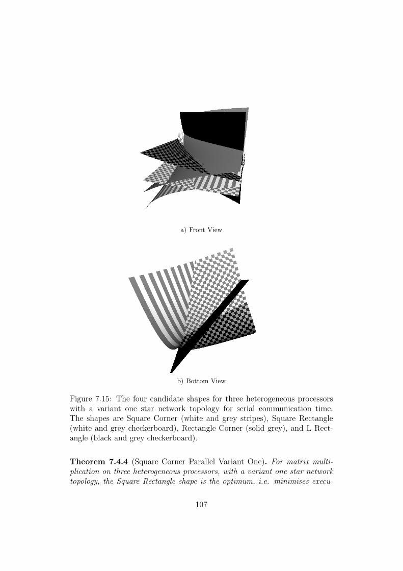
a) Front View
b) Bottom View
Figure 7.15: The four candidate shapes for three heterogeneous processorswith a variant one star network topology for serial communication time.The shapes are Square Corner (white and grey stripes), Square Rectangle(white and grey checkerboard), Rectangle Corner (solid grey), and L Rect-angle (black and grey checkerboard).
Theorem 7.4.4 (Square Corner Parallel Variant One). For matrix multi-plication on three heterogeneous processors, with a variant one star networktopology, the Square Rectangle shape is the optimum, i.e. minimises execu-
107
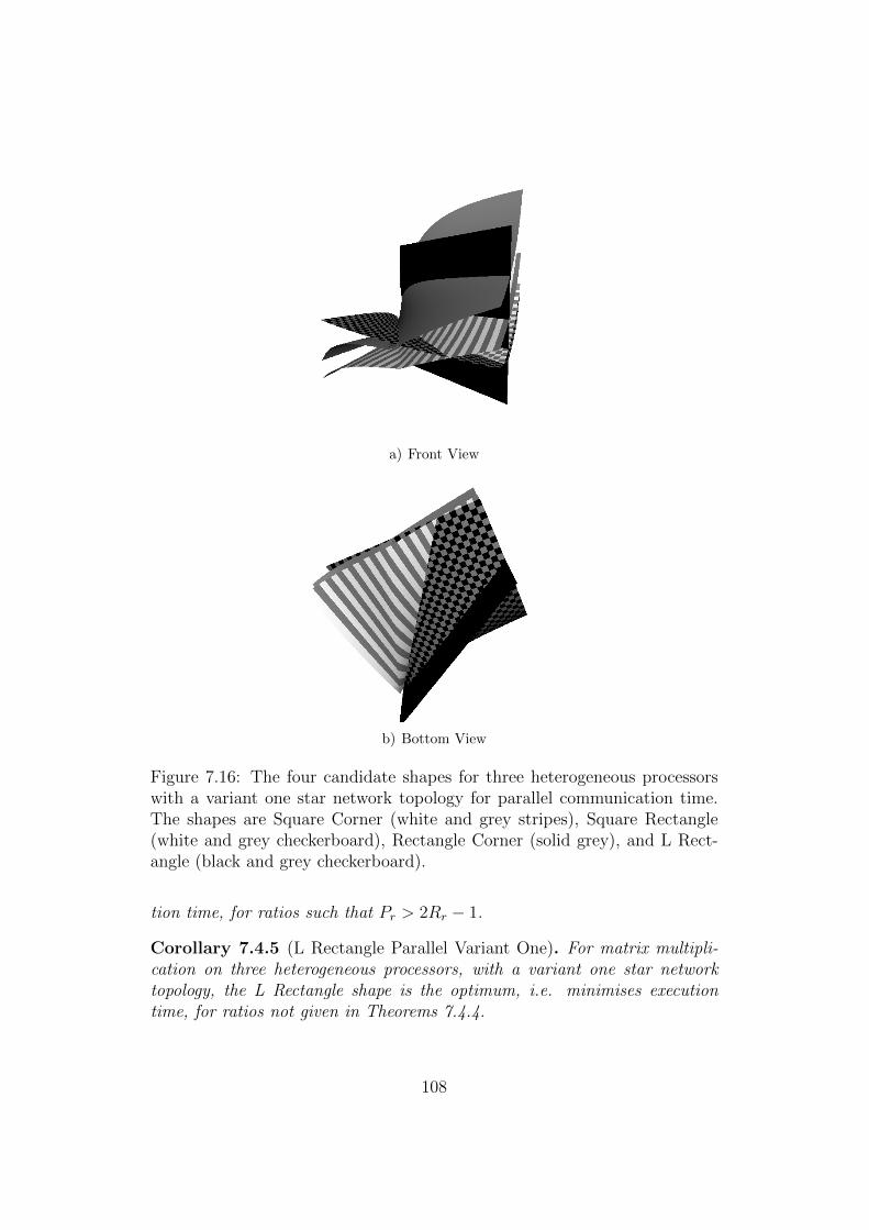
a) Front View
b) Bottom View
Figure 7.16: The four candidate shapes for three heterogeneous processorswith a variant one star network topology for parallel communication time.The shapes are Square Corner (white and grey stripes), Square Rectangle(white and grey checkerboard), Rectangle Corner (solid grey), and L Rect-angle (black and grey checkerboard).
tion time, for ratios such that Pr > 2Rr − 1.
Corollary 7.4.5 (L Rectangle Parallel Variant One). For matrix multipli-cation on three heterogeneous processors, with a variant one star networktopology, the L Rectangle shape is the optimum, i.e. minimises executiontime, for ratios not given in Theorems 7.4.4.
108
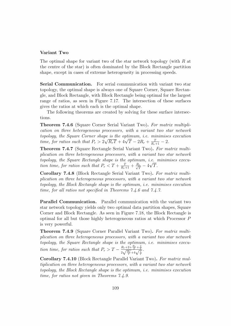
Variant Two
The optimal shape for variant two of the star network topology (with R atthe centre of the star) is often dominated by the Block Rectangle partitionshape, except in cases of extreme heterogeneity in processing speeds.
Serial Communication. For serial communication with variant two startopology, the optimal shape is always one of Square Corner, Square Rectan-gle, and Block Rectangle, with Block Rectangle being optimal for the largestrange of ratios, as seen in Figure 7.17. The intersection of these surfacesgives the ratios at which each is the optimal shape.
The following theorems are created by solving for these surface intersec-tions.
Theorem 7.4.6 (Square Corner Serial Variant Two). For matrix multipli-cation on three heterogeneous processors, with a variant two star networktopology, the Square Corner shape is the optimum, i.e. minimises executiontime, for ratios such that Pr > 2
√RrT + 4
√T − 2Rr + T
Rr+1− 2.
Theorem 7.4.7 (Square Rectangle Serial Variant Two). For matrix multi-plication on three heterogeneous processors, with a variant two star networktopology, the Square Rectangle shape is the optimum, i.e. minimises execu-tion time, for ratios such that Pr < T + T
Rr+1+ Rr√
T− 4√T .
Corollary 7.4.8 (Block Rectangle Serial Variant Two). For matrix multi-plication on three heterogeneous processors, with a variant two star networktopology, the Block Rectangle shape is the optimum, i.e. minimises executiontime, for all ratios not specified in Theorems 7.4.6 and 7.4.7.
Parallel Communication. Parallel communication with the variant twostar network topology yields only two optimal data partition shapes, SquareCorner and Block Rectangle. As seen in Figure 7.18, the Block Rectangle isoptimal for all but those highly heterogeneous ratios at which Processor Pis very powerful.
Theorem 7.4.9 (Square Corner Parallel Variant Two). For matrix multi-plication on three heterogeneous processors, with a variant two star networktopology, the Square Rectangle shape is the optimum, i.e. minimises execu-
tion time, for ratios such that Pr > T − Rr+2+RrT
+ 2T
2√
RrT
+4√
1T
.
Corollary 7.4.10 (Block Rectangle Parallel Variant Two). For matrix mul-tiplication on three heterogeneous processors, with a variant two star networktopology, the Block Rectangle shape is the optimum, i.e. minimises executiontime, for ratios not given in Theorems 7.4.9.
109
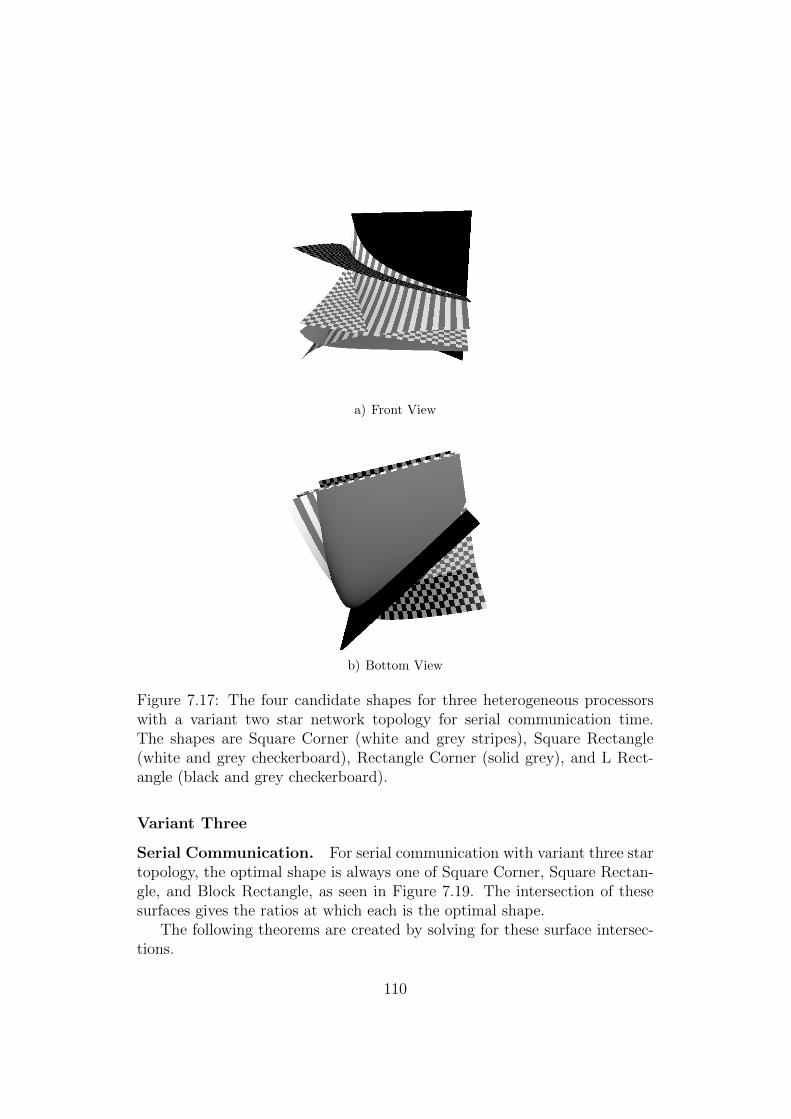
a) Front View
b) Bottom View
Figure 7.17: The four candidate shapes for three heterogeneous processorswith a variant two star network topology for serial communication time.The shapes are Square Corner (white and grey stripes), Square Rectangle(white and grey checkerboard), Rectangle Corner (solid grey), and L Rect-angle (black and grey checkerboard).
Variant Three
Serial Communication. For serial communication with variant three startopology, the optimal shape is always one of Square Corner, Square Rectan-gle, and Block Rectangle, as seen in Figure 7.19. The intersection of thesesurfaces gives the ratios at which each is the optimal shape.
The following theorems are created by solving for these surface intersec-tions.
110
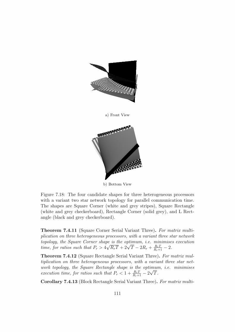
a) Front View
b) Bottom View
Figure 7.18: The four candidate shapes for three heterogeneous processorswith a variant two star network topology for parallel communication time.The shapes are Square Corner (white and grey stripes), Square Rectangle(white and grey checkerboard), Rectangle Corner (solid grey), and L Rect-angle (black and grey checkerboard).
Theorem 7.4.11 (Square Corner Serial Variant Three). For matrix multi-plication on three heterogeneous processors, with a variant three star networktopology, the Square Corner shape is the optimum, i.e. minimises executiontime, for ratios such that Pr > 4
√RrT + 2
√T − 2Rr + RrT
Rr+1− 2.
Theorem 7.4.12 (Square Rectangle Serial Variant Three). For matrix mul-tiplication on three heterogeneous processors, with a variant three star net-work topology, the Square Rectangle shape is the optimum, i.e. minimisesexecution time, for ratios such that Pr < 1 + RrT
Rr+1− 2√T .
Corollary 7.4.13 (Block Rectangle Serial Variant Three). For matrix multi-
111
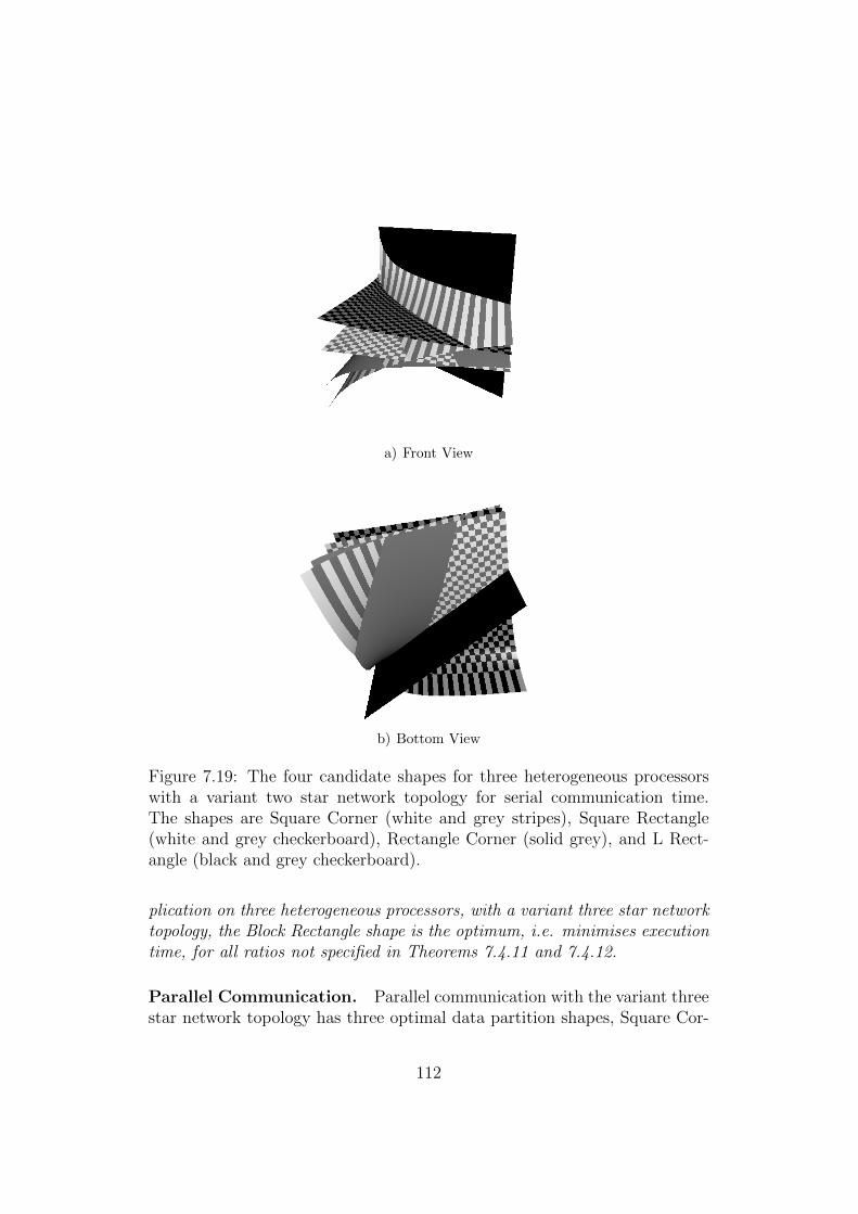
a) Front View
b) Bottom View
Figure 7.19: The four candidate shapes for three heterogeneous processorswith a variant two star network topology for serial communication time.The shapes are Square Corner (white and grey stripes), Square Rectangle(white and grey checkerboard), Rectangle Corner (solid grey), and L Rect-angle (black and grey checkerboard).
plication on three heterogeneous processors, with a variant three star networktopology, the Block Rectangle shape is the optimum, i.e. minimises executiontime, for all ratios not specified in Theorems 7.4.11 and 7.4.12.
Parallel Communication. Parallel communication with the variant threestar network topology has three optimal data partition shapes, Square Cor-
112
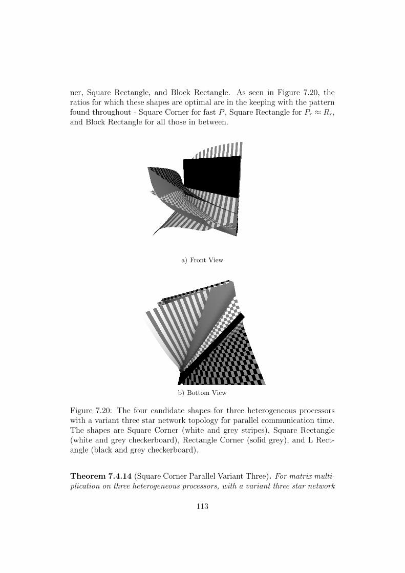
ner, Square Rectangle, and Block Rectangle. As seen in Figure 7.20, theratios for which these shapes are optimal are in the keeping with the patternfound throughout - Square Corner for fast P , Square Rectangle for Pr ≈ Rr,and Block Rectangle for all those in between.
a) Front View
b) Bottom View
Figure 7.20: The four candidate shapes for three heterogeneous processorswith a variant three star network topology for parallel communication time.The shapes are Square Corner (white and grey stripes), Square Rectangle(white and grey checkerboard), Rectangle Corner (solid grey), and L Rect-angle (black and grey checkerboard).
Theorem 7.4.14 (Square Corner Parallel Variant Three). For matrix multi-plication on three heterogeneous processors, with a variant three star network
113
topology, the Square Corner shape is the optimum, i.e. minimises executiontime, for ratios such that Pr > T − (2Rr+1)T
6Rr+1.
Theorem 7.4.15 (Square Rectangle Parallel Variant Three). For matrixmultiplication on three heterogeneous processors, with a variant three starnetwork topology, the Square Rectangle shape is the optimum, i.e. minimisesexecution time, for ratios such that Pr >
3Rr
2+ Rr
2√T−√T + 1.
Corollary 7.4.16 (Block Rectangle Parallel Variant Three). For matrixmultiplication on three heterogeneous processors, with a variant three starnetwork topology, the Block Rectangle shape is the optimum, i.e. minimisesexecution time, for ratios not given in Theorems 7.4.14 and 7.4.15.
7.5 Conclusion
The overwhelming conclusion when considering data partitioning shapes onthree heterogeneous processors is that while the traditional two dimensionalrectangular shape is the ubiquitous for good reason, the novel non-rectangularhave significant advantages, especially as the level of heterogeneity increases.
In the fully connected network topology, the three optimal shapes formedthe same pattern for all algorithms considered. The Square Corner is suitedto a single fast processor, the Square Rectangle to two fast processors, andthe Block Rectangle to everything in between.
More interestingly, the exploration of the star topologies gives insight intowhat happens when the complexity of the model is increased. Rather thanfavour the traditional 2D decomposition, new candidates began to vie foroptimality. This should only reinforce the contention that a single blanketpartition shape (Block Rectangle) is not adequate when considering the widevariability in system parameters in real life heterogeneous systems. Manyother shapes are superior to this, and for some variants in topology thetraditional Block Rectangle is not even a contender for the optimal shape.For each nuance in a given system, the Push Technique can be extended toprovide insight into the optimum shape.
114
Chapter 8
Local Search Optimisations
This chapter will compare and contrast the Push Technique with other localsearch methods, with a focus on simulated annealing. The Push Technique isof similar computational complexity, and produces all possible output datapartition shapes. Simulated annealing experimental results are given, whichreinforce the completeness of the Push Technique results.
8.1 Description of Local Search
Local search is a method for solving computationally intensive optimisationproblems. As previously discussed, the more limited problem of optimallypartitioning heterogeneous rectangles is NP -Complete.
In general, in local search each possible solution has some associatedcost, and the aim is to minimise this cost. Each solution is part of a local“neighbourhood”, which is the area searched for the local minima [64]. Theinitial solution is repeatedly replaced with a solution in the neighbourhoodwith a lower cost. At some point, no neighbouring solution has a lower costthan the one found, and this is the local minimum.
A variety of algorithms operate in this manner such as Hill Climbing,Simulated Annealing, Tabu Search, and Reactive Search.
8.2 Simulated Annealing
In the literature, simulated annealing is a popular choice for local searchalgorithms. It allows the discovery of a variety of local minima within a largesearch space. At the start of the process, an initial solution is swapped withneighbouring solutions, even if those solutions provide an increased cost. Asthe local search progresses, or “cools”, the swaps with neighbouring solutions
115
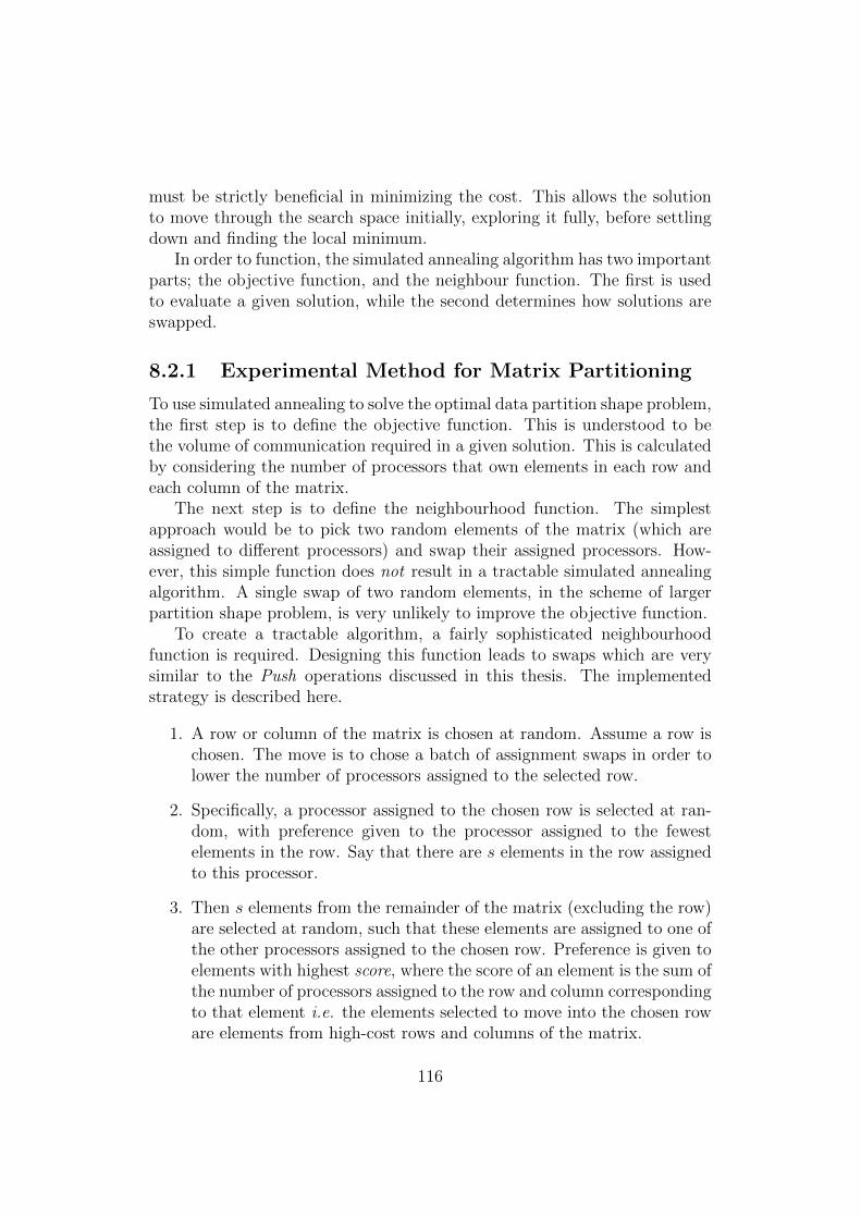
must be strictly beneficial in minimizing the cost. This allows the solutionto move through the search space initially, exploring it fully, before settlingdown and finding the local minimum.
In order to function, the simulated annealing algorithm has two importantparts; the objective function, and the neighbour function. The first is usedto evaluate a given solution, while the second determines how solutions areswapped.
8.2.1 Experimental Method for Matrix Partitioning
To use simulated annealing to solve the optimal data partition shape problem,the first step is to define the objective function. This is understood to bethe volume of communication required in a given solution. This is calculatedby considering the number of processors that own elements in each row andeach column of the matrix.
The next step is to define the neighbourhood function. The simplestapproach would be to pick two random elements of the matrix (which areassigned to different processors) and swap their assigned processors. How-ever, this simple function does not result in a tractable simulated annealingalgorithm. A single swap of two random elements, in the scheme of largerpartition shape problem, is very unlikely to improve the objective function.
To create a tractable algorithm, a fairly sophisticated neighbourhoodfunction is required. Designing this function leads to swaps which are verysimilar to the Push operations discussed in this thesis. The implementedstrategy is described here.
1. A row or column of the matrix is chosen at random. Assume a row ischosen. The move is to chose a batch of assignment swaps in order tolower the number of processors assigned to the selected row.
2. Specifically, a processor assigned to the chosen row is selected at ran-dom, with preference given to the processor assigned to the fewestelements in the row. Say that there are s elements in the row assignedto this processor.
3. Then s elements from the remainder of the matrix (excluding the row)are selected at random, such that these elements are assigned to one ofthe other processors assigned to the chosen row. Preference is given toelements with highest score, where the score of an element is the sum ofthe number of processors assigned to the row and column correspondingto that element i.e. the elements selected to move into the chosen roware elements from high-cost rows and columns of the matrix.
116
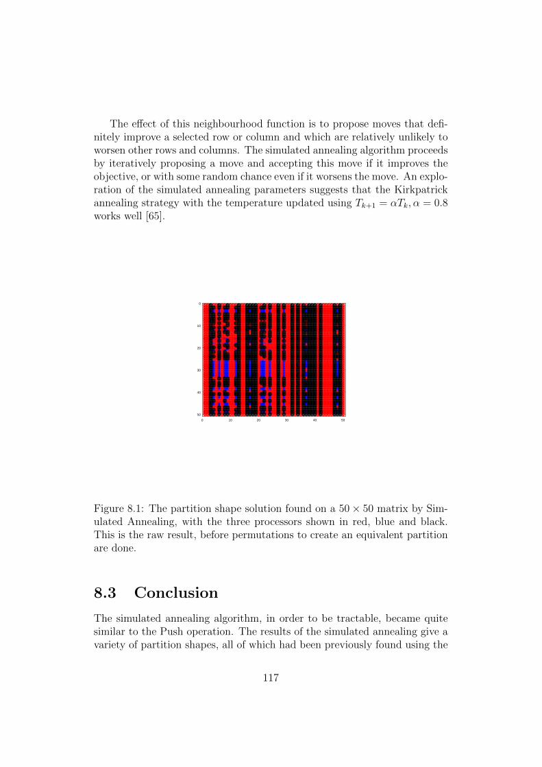
The effect of this neighbourhood function is to propose moves that defi-nitely improve a selected row or column and which are relatively unlikely toworsen other rows and columns. The simulated annealing algorithm proceedsby iteratively proposing a move and accepting this move if it improves theobjective, or with some random chance even if it worsens the move. An explo-ration of the simulated annealing parameters suggests that the Kirkpatrickannealing strategy with the temperature updated using Tk+1 = αTk, α = 0.8works well [65].
0 10 20 30 40 50
0
10
20
30
40
50
Figure 8.1: The partition shape solution found on a 50× 50 matrix by Sim-ulated Annealing, with the three processors shown in red, blue and black.This is the raw result, before permutations to create an equivalent partitionare done.
8.3 Conclusion
The simulated annealing algorithm, in order to be tractable, became quitesimilar to the Push operation. The results of the simulated annealing give avariety of partition shapes, all of which had been previously found using the
117
0 10 20 30 40 50
0
10
20
30
40
50
Figure 8.2: The solution found on a 50× 50 matrix by Simulated Annealing.This is the final result, after permutations to create an equivalent partitionare done. All rows and columns containing three processors are moved to thefar left/top, then all rows and columns containing two processors, and so on.
Push. For example, in Figures 8.1 and 8.2, the results of a single run of thesimulated annealing are given. At first, the results look unfamiliar, as thePush technique has a natural tendency towards a processor being assignedcontiguous elements. However, a simple permutation of the matrix givesa shape that is recognisable as being in the same archetype as the SquareRectangle. This permutation involves swapping rows or columns, and doesnot affect the cost of the solution found.
The Push Technique is similar to local search. It starts with a randomsolution, and moves between solutions according to a predetermined functionto arrive at some final result which is a local minimum. The Push Techniquefinds all possible local minima, also called candidates.
118
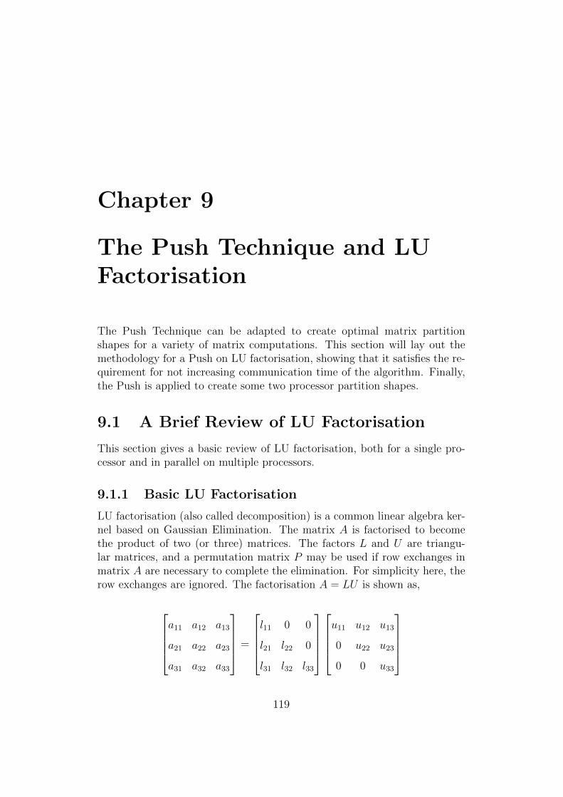
Chapter 9
The Push Technique and LUFactorisation
The Push Technique can be adapted to create optimal matrix partitionshapes for a variety of matrix computations. This section will lay out themethodology for a Push on LU factorisation, showing that it satisfies the re-quirement for not increasing communication time of the algorithm. Finally,the Push is applied to create some two processor partition shapes.
9.1 A Brief Review of LU Factorisation
This section gives a basic review of LU factorisation, both for a single pro-cessor and in parallel on multiple processors.
9.1.1 Basic LU Factorisation
LU factorisation (also called decomposition) is a common linear algebra ker-nel based on Gaussian Elimination. The matrix A is factorised to becomethe product of two (or three) matrices. The factors L and U are triangu-lar matrices, and a permutation matrix P may be used if row exchanges inmatrix A are necessary to complete the elimination. For simplicity here, therow exchanges are ignored. The factorisation A = LU is shown as,
a11 a12 a13
a21 a22 a23
a31 a32 a33
=
l11 0 0
l21 l22 0
l31 l32 l33
u11 u12 u13
0 u22 u23
0 0 u33
119
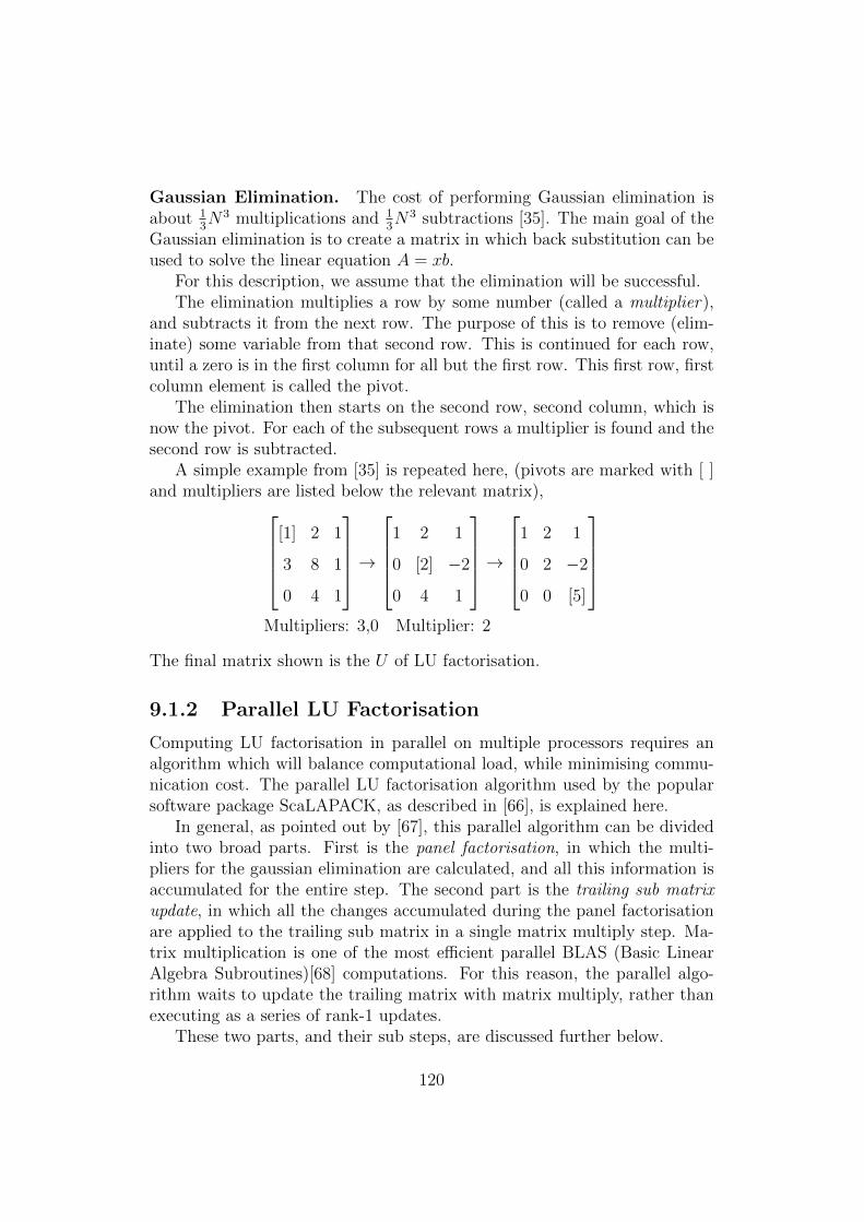
Gaussian Elimination. The cost of performing Gaussian elimination isabout 1
3N3 multiplications and 1
3N3 subtractions [35]. The main goal of the
Gaussian elimination is to create a matrix in which back substitution can beused to solve the linear equation A = xb.
For this description, we assume that the elimination will be successful.The elimination multiplies a row by some number (called a multiplier),
and subtracts it from the next row. The purpose of this is to remove (elim-inate) some variable from that second row. This is continued for each row,until a zero is in the first column for all but the first row. This first row, firstcolumn element is called the pivot.
The elimination then starts on the second row, second column, which isnow the pivot. For each of the subsequent rows a multiplier is found and thesecond row is subtracted.
A simple example from [35] is repeated here, (pivots are marked with [ ]and multipliers are listed below the relevant matrix),
[1] 2 1
3 8 1
0 4 1
→
1 2 1
0 [2] −2
0 4 1
→
1 2 1
0 2 −2
0 0 [5]
Multipliers: 3,0 Multiplier: 2
The final matrix shown is the U of LU factorisation.
9.1.2 Parallel LU Factorisation
Computing LU factorisation in parallel on multiple processors requires analgorithm which will balance computational load, while minimising commu-nication cost. The parallel LU factorisation algorithm used by the popularsoftware package ScaLAPACK, as described in [66], is explained here.
In general, as pointed out by [67], this parallel algorithm can be dividedinto two broad parts. First is the panel factorisation, in which the multi-pliers for the gaussian elimination are calculated, and all this information isaccumulated for the entire step. The second part is the trailing sub matrixupdate, in which all the changes accumulated during the panel factorisationare applied to the trailing sub matrix in a single matrix multiply step. Ma-trix multiplication is one of the most efficient parallel BLAS (Basic LinearAlgebra Subroutines)[68] computations. For this reason, the parallel algo-rithm waits to update the trailing matrix with matrix multiply, rather thanexecuting as a series of rank-1 updates.
These two parts, and their sub steps, are discussed further below.
120
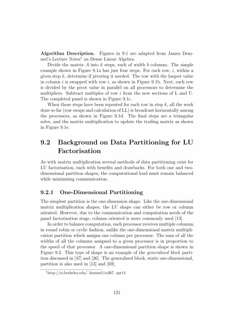
Algorithm Description. Figures in 9.1 are adapted from James Dem-mel’s Lecture Notes1 on Dense Linear Algebra.
Divide the matrix A into k steps, each of width b columns. The simpleexample shown in Figure 9.1a has just four steps. For each row, i, within agiven step k, determine if pivoting it needed. The row with the largest valuein column i is swapped with row i, as shown in Figure 9.1b. Next, each rowis divided by the pivot value in parallel on all processors to determine themultipliers. Subtract multiples of row i from the new sections of L and U.The completed panel is shown in Figure 9.1c.
When those steps have been repeated for each row in step k, all the workdone so far (row swaps and calculation of LL) is broadcast horizontally amongthe processors, as shown in Figure 9.1d. The final steps are a triangularsolve, and the matrix multiplication to update the trailing matrix as shownin Figure 9.1e.
9.2 Background on Data Partitioning for LU
Factorisation
As with matrix multiplication several methods of data partitioning exist forLU factorisation, each with benefits and drawbacks. For both one and two-dimensional partition shapes, the computational load must remain balancedwhile minimising communication.
9.2.1 One-Dimensional Partitioning
The simplest partition is the one-dimension shape. Like the one-dimensionalmatrix multiplication shapes, the LU shape can either be row or columnoriented. However, due to the communication and computation needs of thepanel factorisation stage, column oriented is more commonly used [13].
In order to balance computation, each processor receives multiple columns,in round robin or cyclic fashion, unlike the one-dimensional matrix multipli-cation partition which assigns one column per processor. The sum of all thewidths of all the columns assigned to a given processor is in proportion tothe speed of that processor. A one-dimensional partition shape is shown inFigure 9.2. This type of shape is an example of the generalised block parti-tion discussed in [47] and [26]. The generalised block, static one-dimensional,partition is also used in [13] and [69].
1http://cs.berkeley.edu/˜demmel/cs267 spr14
121
b
b
a) k = 4 steps
i
(i,i)
b) Search column for pivot and swap
c) Compute multipliers and sub-tract
d) Send LL horizontally and dotriangular solve
1
2
e) Matrix Multiply (Submatrix = Sub-matrix - (Matrx 1 * Matrix 2)
Figure 9.1: LU factorisation parallel algorithm. White is the current step,light grey the completed factorisation, and dark grey the trailing submatrixto be updated/factorised.
122
Figure 9.2: A one dimensional, column oriented, partition shape for LUfactorisation on three heterogeneous processors (shown in white, grey, andblack).
In addition to the generalised block, two other algorithms for one-dimensionalLU partitions exist. First is the Dynamic Programming [45, 70] method,which distributes column panels to processors for execution. This algorithmreturns an optimal solution, but does not scale well for non-constant perfor-mance models. The second is the Reverse Algorithm [71, 72]. This algorithmalso provides an optimal solution, at somewhat worse complexity, with thebenefit of an easier extension to non-constant performance models of proces-sor speed.
9.2.2 Two-Dimensional Partitioning
Two-dimensional partitioning for LU factorisation is not common amongtwo and three processor systems, due to the considerations of computationalload. However, the same two-dimensional partitions used for four and moreprocessors could be used to partition three heterogeneous processors.
A common one of these is the two-dimensional cyclic layout as shown inFigure 9.3.
9.3 Applying Push to LU Factorisation
This section will show how the Push Technique may be applied to LU factori-sation, specifically considering the issues of maintaining a balanced compu-tational load while minimising communication. To use the Push under theseconstraints involves a modified methodology, which is also described. Finally,
123
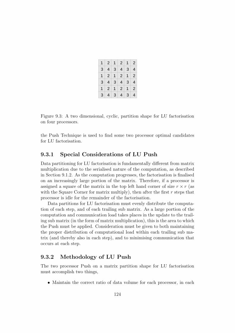
1 2
3 4
1 2
3 4
1 2
3 4
1 2
3 4
1 2
3 4
1 2
3 4
1 2
3 4
1 2
3 4
1 2
3 4
Figure 9.3: A two dimensional, cyclic, partition shape for LU factorisationon four processors.
the Push Technique is used to find some two processor optimal candidatesfor LU factorisation.
9.3.1 Special Considerations of LU Push
Data partitioning for LU factorisation is fundamentally different from matrixmultiplication due to the serialised nature of the computation, as describedin Section 9.1.2. As the computation progresses, the factorisation is finalisedon an increasingly large portion of the matrix. Therefore, if a processor isassigned a square of the matrix in the top left hand corner of size r × r (aswith the Square Corner for matrix multiply), then after the first r steps thatprocessor is idle for the remainder of the factorisation.
Data partitions for LU factorisation must evenly distribute the computa-tion of each step, and of each trailing sub matrix. As a large portion of thecomputation and communication load takes places in the update to the trail-ing sub matrix (in the form of matrix multiplication), this is the area to whichthe Push must be applied. Consideration must be given to both maintainingthe proper distribution of computational load within each trailing sub ma-trix (and thereby also in each step), and to minimising communication thatoccurs at each step.
9.3.2 Methodology of LU Push
The two processor Push on a matrix partition shape for LU factorisationmust accomplish two things,
• Maintain the correct ratio of data volume for each processor, in each
124
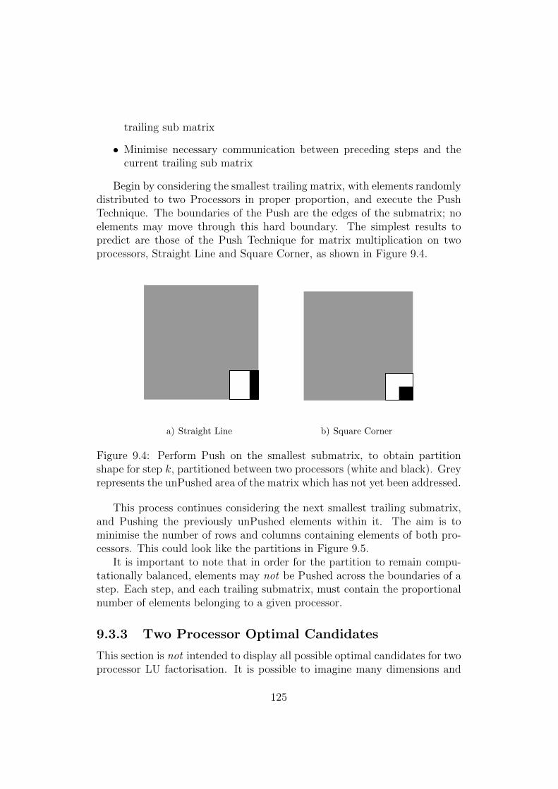
trailing sub matrix
• Minimise necessary communication between preceding steps and thecurrent trailing sub matrix
Begin by considering the smallest trailing matrix, with elements randomlydistributed to two Processors in proper proportion, and execute the PushTechnique. The boundaries of the Push are the edges of the submatrix; noelements may move through this hard boundary. The simplest results topredict are those of the Push Technique for matrix multiplication on twoprocessors, Straight Line and Square Corner, as shown in Figure 9.4.
a) Straight Line b) Square Corner
Figure 9.4: Perform Push on the smallest submatrix, to obtain partitionshape for step k, partitioned between two processors (white and black). Greyrepresents the unPushed area of the matrix which has not yet been addressed.
This process continues considering the next smallest trailing submatrix,and Pushing the previously unPushed elements within it. The aim is tominimise the number of rows and columns containing elements of both pro-cessors. This could look like the partitions in Figure 9.5.
It is important to note that in order for the partition to remain compu-tationally balanced, elements may not be Pushed across the boundaries of astep. Each step, and each trailing submatrix, must contain the proportionalnumber of elements belonging to a given processor.
9.3.3 Two Processor Optimal Candidates
This section is not intended to display all possible optimal candidates for twoprocessor LU factorisation. It is possible to imagine many dimensions and
125
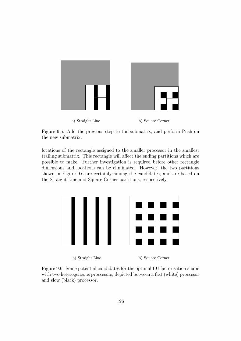
a) Straight Line b) Square Corner
Figure 9.5: Add the previous step to the submatrix, and perform Push onthe new submatrix.
locations of the rectangle assigned to the smaller processor in the smallesttrailing submatrix. This rectangle will affect the ending partitions which arepossible to make. Further investigation is required before other rectangledimensions and locations can be eliminated. However, the two partitionsshown in Figure 9.6 are certainly among the candidates, and are based onthe Straight Line and Square Corner partitions, respectively.
a) Straight Line b) Square Corner
Figure 9.6: Some potential candidates for the optimal LU factorisation shapewith two heterogeneous processors, depicted between a fast (white) processorand slow (black) processor.
126
Chapter 10
Further Work
While the work of the previous chapters has made significant progress de-termining optimal data partitioning shapes for matrix computations, thereare a variety of ways this work could be further expanded. First, the mostobvious addition to this work is to increase the number of processors to whichit is applicable. A general roadmap to using the Push Technique on four andmore processors has been provided, however, this section further expands onthe possibilities and challenges in this future work.
The concept of the abstract processor was strictly defined in a simplemanner, to provide a base case that might be applicable to the largest numbersystems possible. By increasing the number of metrics used to describe anabstract processor in terms of computation, communication, and memory,the boundaries at which each candidate becomes the optimal shape could befurther refined for particular system types.
Finally, the Push Technique itself is a powerful tool that, with somechanges to the performance model of the optimisation metric, can be appliedto matrix computations in general.
10.1 Arbitrary Number of Processors
This thesis does not exhaust the number of processors for which the PushTechnique is a useful tool. Using the Push DFA to implement an extensionto the software tool for four and more processors is underway. However, it isnot expected that the Push Technique be a feasible tool beyond some numberof processors, perhaps eight or ten.
To consider the question of an arbitrary number of processors, a formalmethod for using the Push Technique in a hierarchical way would need to bedeveloped. This method would describe the interaction of multiple layers of
127
processing power, and how a Push at one level in the hierarchy would effectthe optimal partition shape at other levels. For example, if at the highestlevel several clusters were used (and due to their computational speeds) theSquare Corner was chosen to distribute the data amongst them, any changein their underlying computational speed (due to change in the optimal datapartition at a lower, node level) could affect the distribution at the higherlevel. This process could be defined in fashion similar to that of the LUfactorisation Push, which starts at the base level and works up to somecomplete partition shape.
This leads naturally to the question of how would non-rectangular parti-tions be divided at the lower levels. The Push Technique should be extendedfor use on non-square matrices, so a non-rectangular matrix could potentiallybe considered two or more non-square rectangular matrices.
10.2 Increasing Complexity of Abstract Pro-
cessor
There are a variety of ways the abstract processor model could be extendedto increase the sensitivity of the model to diverse types of heterogeneousprocessors and networks.
10.2.1 Non-Symmetric Network Topology
The communication interconnect among processors can be widely varied inactual technology (Ethernet, InfiniBand), and in latency and bandwidth asa result of overall network congestion. Throughout this work, it has been as-sumed that communication is symmetric and can be represented by a singleconstant bandwidth, β. In future work, non-symmetric links could be repre-sented using a unique constant for each link (including a constant of zero fornon-existent links). If p processors are connected by nn−1
2links, then there
exist n(n−1) bandwidth variables labelled pi→j for communication travellingfrom Processor pi to Processor pj.
As with the optimal rectangle tiling problem, the optimal distributionof data on a heterogeneous network has also been shown to have cases ofNP -completeness [73].
10.2.2 Computational Performance Model
The abstract processor is currently modelled computationally as a singleinteger number, expressed in the form of a ratio in proportion to the total
128
power of the system. However, this constant performance model could bereplaced with a more complex functional performance model, based on theoverall problem size (matrix size). A functional model would account for thechanges that occur, as the matrix size grows, in the performance of differentprocessors. While the addition of a functional performance model would notchange the candidate shapes, it could alter the boundaries at which eachcandidate is the optimum.
Other options for growth in computational modelling include further pa-rameterising of the basic unit of computation, such as is necessary for othermatrix computations.
10.2.3 Memory Model
Related to the computational model, as it is often the reason for varyingcomputational performance, is the memory model. It is well known thatdifferent processor types possess significantly different amounts of memory,especially in comparison to their respective throughput in FLOPs.
10.3 Push Technique and Other Matrix Com-
putations
The Push Technique has been thoroughly investigated for matrix multipli-cation, and a methodology for use with LU factorisation has been given.However, other matrix computations pose some difficult challenges.
The key idea will be to identify those performance metrics of a givenmatrix computation which can be incrementally altered to achieve an op-timal ending shape. Some possibilities for extension lie in other commonlinear algebra kernels in ScaLAPACK such as QR factorisation and otherdecomposition problems.
However, it is worth mentioning that the work done in this thesis withmatrix multiplication could give insights into any matrix computation whichuses matrix multiply in its parallel algorithm for the BLAS-3 speedup (asLU factorisation does).
129
Chapter 11
Conclusions
This thesis has outlined a solution to a particularly thorny problem - theoptimal data partitioning for matrix computation for heterogeneous proces-sors. Candidates for the optimal shape were found using the new PushTechnique, which included unconventional non-rectangular shapes. Severalof these shapes are indeed optimal for certain system characteristics in re-gards to ratios of computational power and communication speed.
11.1 The Push Technique
The Push Technique is a simple but powerful method of obtaining partitionshapes. Using small, incremental changes to a data partition (each of whichimproves the partition metrics of communication time) the end result ofthe Push DFA is a finite set of candidate partition shapes. These candidateshapes may be compared directly, according to their performance models andalgorithms, to determine which of the candidates is indeed the optimum.
The Push has several distinct advantages over typical methods for findingthe partition shapes. The Push Technique:
• finds all candidate shapes, especially unexpected or novel shapes (suchas Square Rectangle)
• ensures that candidate shapes are potentially optimally (as opposed tosub-optimal by definition)
• needs only to be thoroughly used once for each number of processors(to find all possible candidates)
• complexity of the DFA scales well with problem size
130
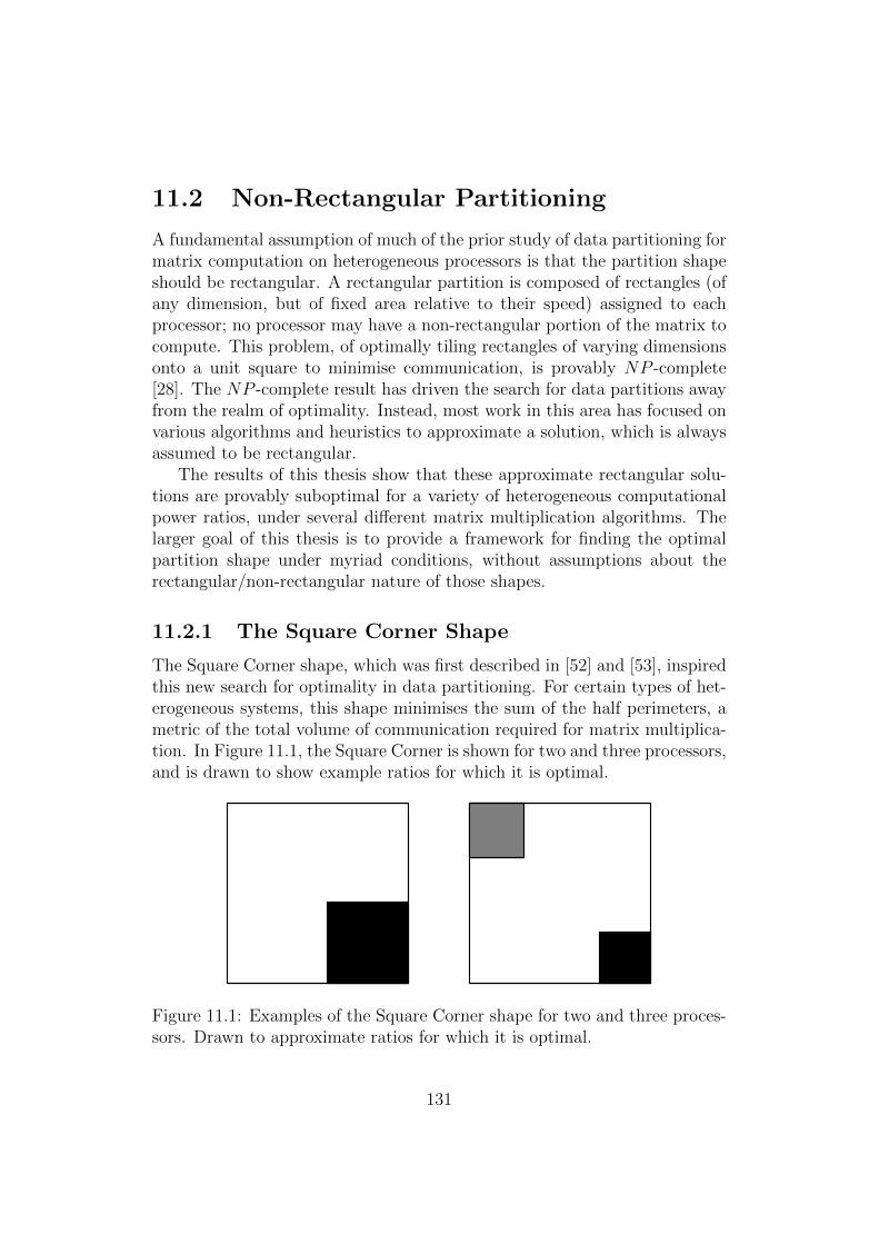
11.2 Non-Rectangular Partitioning
A fundamental assumption of much of the prior study of data partitioning formatrix computation on heterogeneous processors is that the partition shapeshould be rectangular. A rectangular partition is composed of rectangles (ofany dimension, but of fixed area relative to their speed) assigned to eachprocessor; no processor may have a non-rectangular portion of the matrix tocompute. This problem, of optimally tiling rectangles of varying dimensionsonto a unit square to minimise communication, is provably NP -complete[28]. The NP -complete result has driven the search for data partitions awayfrom the realm of optimality. Instead, most work in this area has focused onvarious algorithms and heuristics to approximate a solution, which is alwaysassumed to be rectangular.
The results of this thesis show that these approximate rectangular solu-tions are provably suboptimal for a variety of heterogeneous computationalpower ratios, under several different matrix multiplication algorithms. Thelarger goal of this thesis is to provide a framework for finding the optimalpartition shape under myriad conditions, without assumptions about therectangular/non-rectangular nature of those shapes.
11.2.1 The Square Corner Shape
The Square Corner shape, which was first described in [52] and [53], inspiredthis new search for optimality in data partitioning. For certain types of het-erogeneous systems, this shape minimises the sum of the half perimeters, ametric of the total volume of communication required for matrix multiplica-tion. In Figure 11.1, the Square Corner is shown for two and three processors,and is drawn to show example ratios for which it is optimal.
Figure 11.1: Examples of the Square Corner shape for two and three proces-sors. Drawn to approximate ratios for which it is optimal.
131
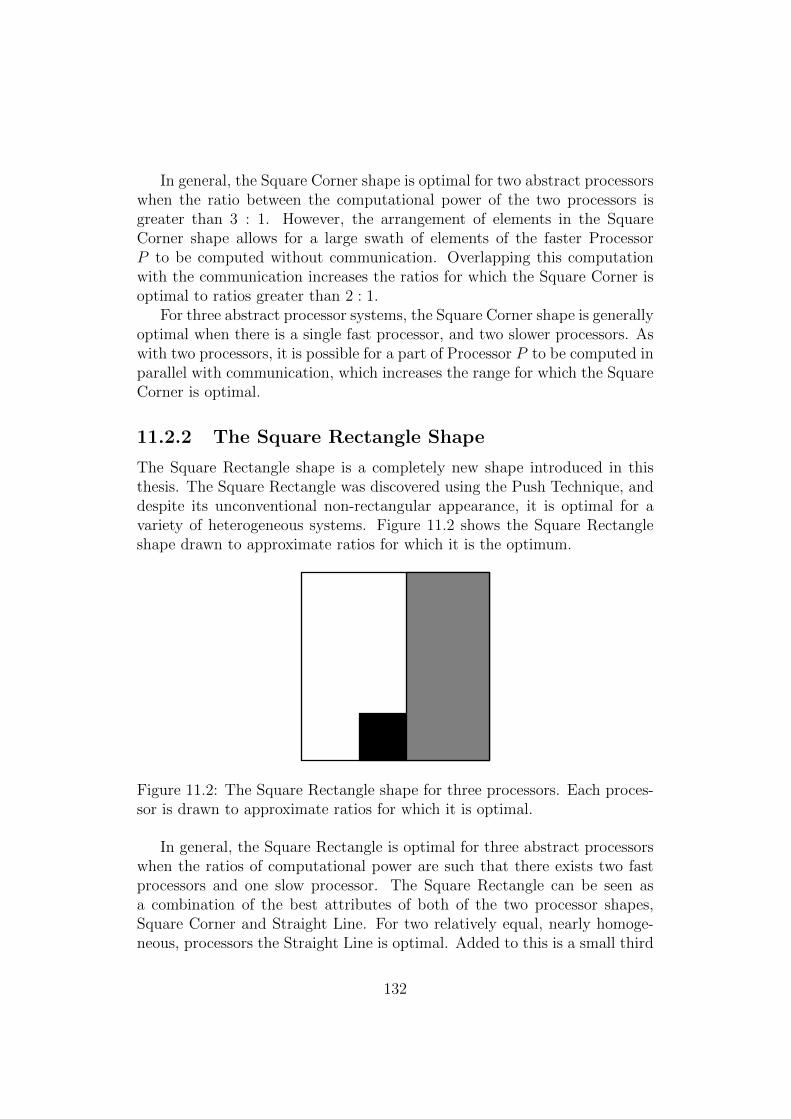
In general, the Square Corner shape is optimal for two abstract processorswhen the ratio between the computational power of the two processors isgreater than 3 : 1. However, the arrangement of elements in the SquareCorner shape allows for a large swath of elements of the faster ProcessorP to be computed without communication. Overlapping this computationwith the communication increases the ratios for which the Square Corner isoptimal to ratios greater than 2 : 1.
For three abstract processor systems, the Square Corner shape is generallyoptimal when there is a single fast processor, and two slower processors. Aswith two processors, it is possible for a part of Processor P to be computed inparallel with communication, which increases the range for which the SquareCorner is optimal.
11.2.2 The Square Rectangle Shape
The Square Rectangle shape is a completely new shape introduced in thisthesis. The Square Rectangle was discovered using the Push Technique, anddespite its unconventional non-rectangular appearance, it is optimal for avariety of heterogeneous systems. Figure 11.2 shows the Square Rectangleshape drawn to approximate ratios for which it is the optimum.
Figure 11.2: The Square Rectangle shape for three processors. Each proces-sor is drawn to approximate ratios for which it is optimal.
In general, the Square Rectangle is optimal for three abstract processorswhen the ratios of computational power are such that there exists two fastprocessors and one slow processor. The Square Rectangle can be seen asa combination of the best attributes of both of the two processor shapes,Square Corner and Straight Line. For two relatively equal, nearly homoge-neous, processors the Straight Line is optimal. Added to this is a small third
132
processor, in the shape of a square to minimise communication with the restof the matrix.
11.3 Pushing the Boundaries: Wider Appli-
cability
While Chapter 10 outlined the limitations of this thesis in terms of numberof processors used (two or three rather than many) and abstract processormodel (basic rather than complex), the overall theme of this thesis is one ofgenerality. The Push Technique, incrementally improving a partition shapeaccording to some metric, was applied to both matrix multiplication and LUfactorisation with good results. To increase the complexity of the abstractprocessor would not change this fundamental result.
Similarly, the three processor case shows the wider applicability of thePush Technique to any arbitrary number of processors. It appears that forany reasonable number of processors, say less than ten, the Push Techniquecould create candidate partitions for sufficiently large enough problem sizes(to allow greater granularity in element movement). Furthermore, the candi-dates created using the Push Technique can be utilised in a hierarchical way,so as to minimise communication for any number of processors.
133
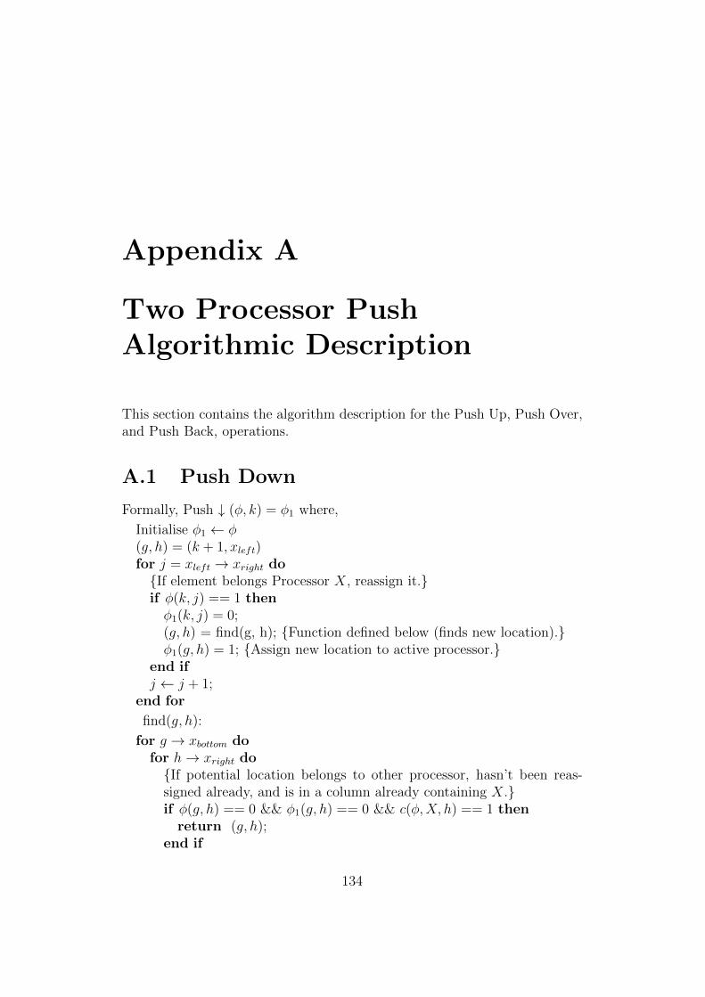
Appendix A
Two Processor PushAlgorithmic Description
This section contains the algorithm description for the Push Up, Push Over,and Push Back, operations.
A.1 Push Down
Formally, Push ↓ (φ, k) = φ1 where,
Initialise φ1 ← φ(g, h) = (k + 1, xleft)for j = xleft → xright do{If element belongs Processor X, reassign it.}if φ(k, j) == 1 thenφ1(k, j) = 0;(g, h) = find(g, h); {Function defined below (finds new location).}φ1(g, h) = 1; {Assign new location to active processor.}
end ifj ← j + 1;
end for
find(g, h):
for g → xbottom dofor h→ xright do{If potential location belongs to other processor, hasn’t been reas-signed already, and is in a column already containing X.}if φ(g, h) == 0 && φ1(g, h) == 0 && c(φ,X, h) == 1 then
return (g, h);end if
134
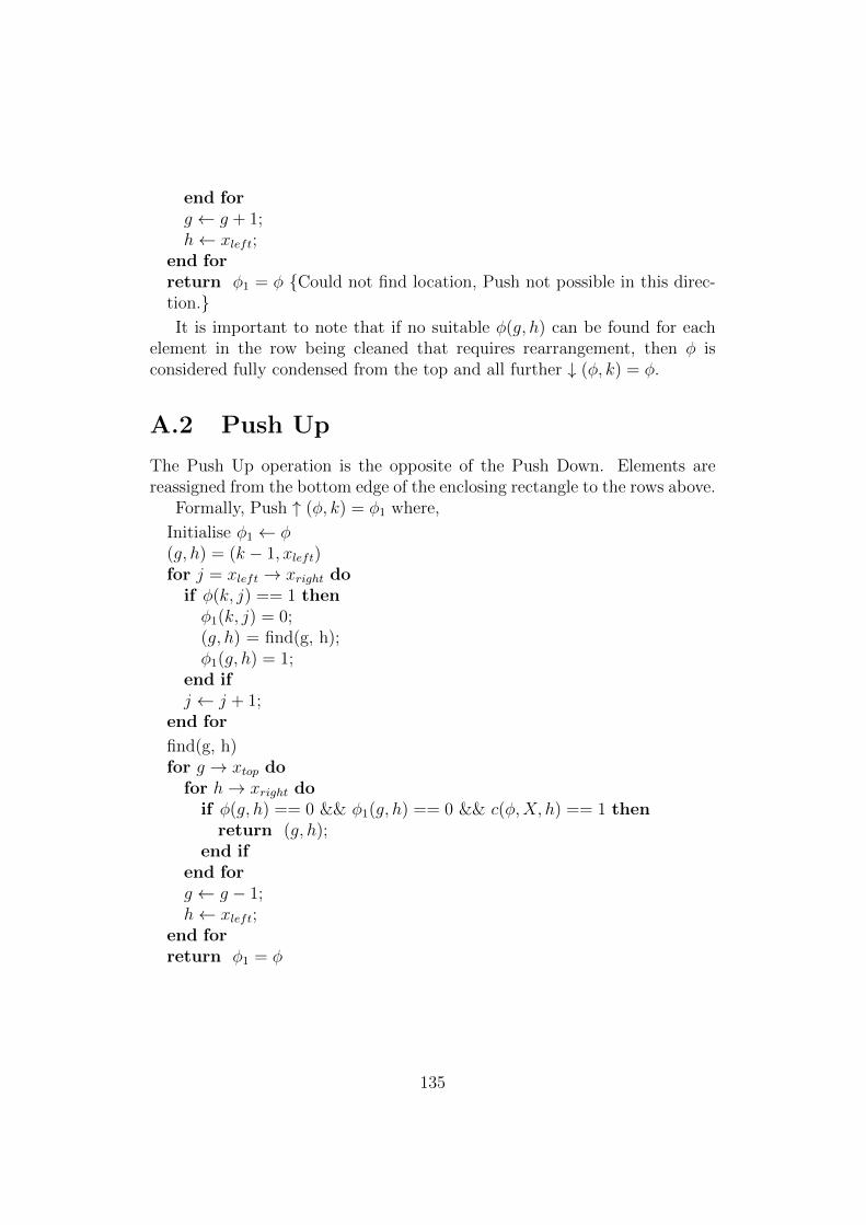
end forg ← g + 1;h← xleft;
end forreturn φ1 = φ {Could not find location, Push not possible in this direc-tion.}It is important to note that if no suitable φ(g, h) can be found for each
element in the row being cleaned that requires rearrangement, then φ isconsidered fully condensed from the top and all further ↓ (φ, k) = φ.
A.2 Push Up
The Push Up operation is the opposite of the Push Down. Elements arereassigned from the bottom edge of the enclosing rectangle to the rows above.
Formally, Push ↑ (φ, k) = φ1 where,
Initialise φ1 ← φ(g, h) = (k − 1, xleft)for j = xleft → xright do
if φ(k, j) == 1 thenφ1(k, j) = 0;(g, h) = find(g, h);φ1(g, h) = 1;
end ifj ← j + 1;
end for
find(g, h)for g → xtop do
for h→ xright doif φ(g, h) == 0 && φ1(g, h) == 0 && c(φ,X, h) == 1 then
return (g, h);end if
end forg ← g − 1;h← xleft;
end forreturn φ1 = φ
135
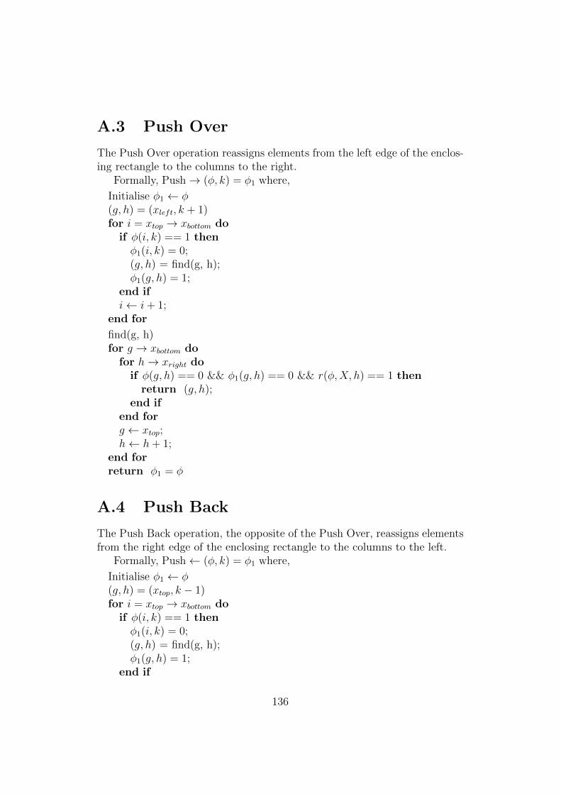
A.3 Push Over
The Push Over operation reassigns elements from the left edge of the enclos-ing rectangle to the columns to the right.
Formally, Push→ (φ, k) = φ1 where,
Initialise φ1 ← φ(g, h) = (xleft, k + 1)for i = xtop → xbottom do
if φ(i, k) == 1 thenφ1(i, k) = 0;(g, h) = find(g, h);φ1(g, h) = 1;
end ifi← i+ 1;
end for
find(g, h)for g → xbottom do
for h→ xright doif φ(g, h) == 0 && φ1(g, h) == 0 && r(φ,X, h) == 1 then
return (g, h);end if
end forg ← xtop;h← h+ 1;
end forreturn φ1 = φ
A.4 Push Back
The Push Back operation, the opposite of the Push Over, reassigns elementsfrom the right edge of the enclosing rectangle to the columns to the left.
Formally, Push← (φ, k) = φ1 where,
Initialise φ1 ← φ(g, h) = (xtop, k − 1)for i = xtop → xbottom do
if φ(i, k) == 1 thenφ1(i, k) = 0;(g, h) = find(g, h);φ1(g, h) = 1;
end if
136
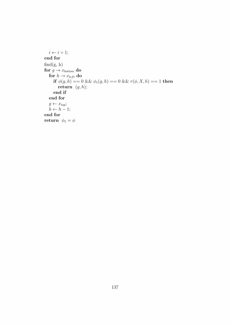
i← i+ 1;end for
find(g, h)for g → xbottom do
for h→ xleft doif φ(g, h) == 0 && φ1(g, h) == 0 && r(φ,X, h) == 1 then
return (g, h);end if
end forg ← xtop;h← h− 1;
end forreturn φ1 = φ
137
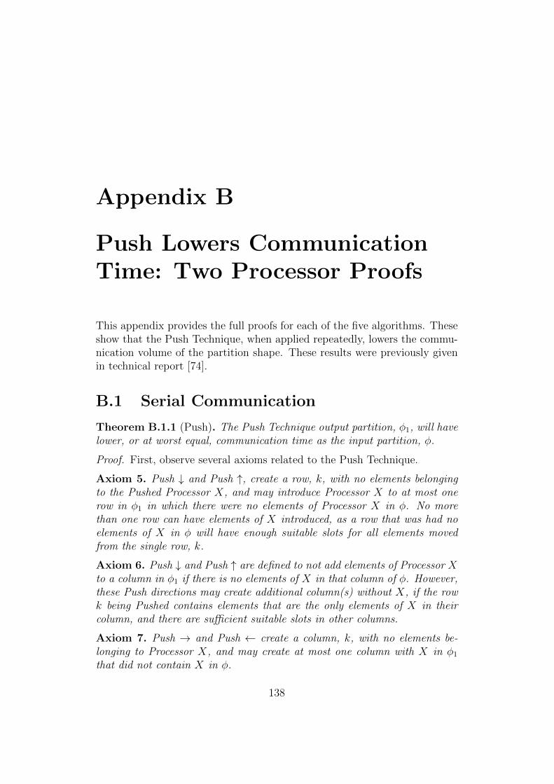
Appendix B
Push Lowers CommunicationTime: Two Processor Proofs
This appendix provides the full proofs for each of the five algorithms. Theseshow that the Push Technique, when applied repeatedly, lowers the commu-nication volume of the partition shape. These results were previously givenin technical report [74].
B.1 Serial Communication
Theorem B.1.1 (Push). The Push Technique output partition, φ1, will havelower, or at worst equal, communication time as the input partition, φ.
Proof. First, observe several axioms related to the Push Technique.
Axiom 5. Push ↓ and Push ↑, create a row, k, with no elements belongingto the Pushed Processor X, and may introduce Processor X to at most onerow in φ1 in which there were no elements of Processor X in φ. No morethan one row can have elements of X introduced, as a row that was had noelements of X in φ will have enough suitable slots for all elements movedfrom the single row, k.
Axiom 6. Push ↓ and Push ↑ are defined to not add elements of Processor Xto a column in φ1 if there is no elements of X in that column of φ. However,these Push directions may create additional column(s) without X, if the rowk being Pushed contains elements that are the only elements of X in theircolumn, and there are sufficient suitable slots in other columns.
Axiom 7. Push → and Push ← create a column, k, with no elements be-longing to Processor X, and may create at most one column with X in φ1
that did not contain X in φ.
138
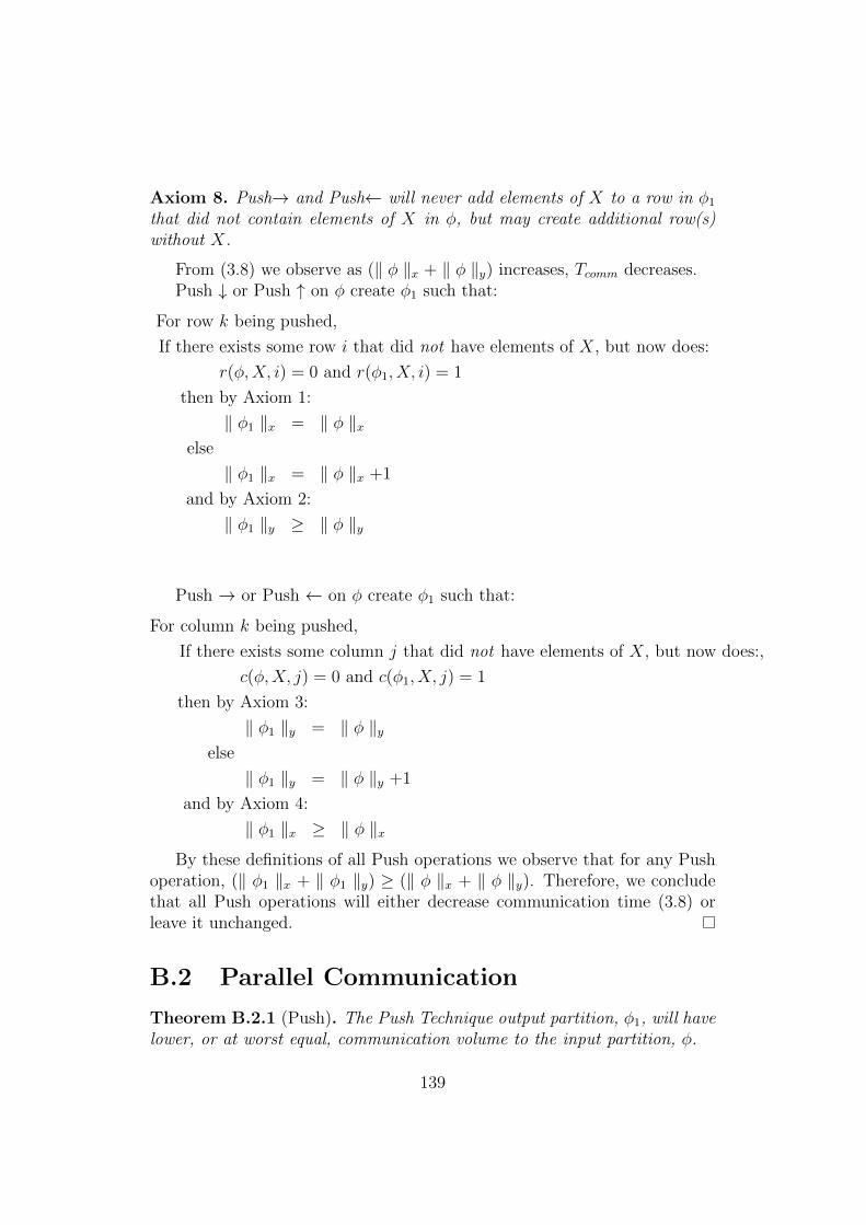
Axiom 8. Push→ and Push← will never add elements of X to a row in φ1
that did not contain elements of X in φ, but may create additional row(s)without X.
From (3.8) we observe as (‖ φ ‖x + ‖ φ ‖y) increases, Tcomm decreases.Push ↓ or Push ↑ on φ create φ1 such that:
For row k being pushed,
If there exists some row i that did not have elements of X, but now does:
r(φ,X, i) = 0 and r(φ1, X, i) = 1
then by Axiom 1:
‖ φ1 ‖x = ‖ φ ‖xelse
‖ φ1 ‖x = ‖ φ ‖x +1
and by Axiom 2:
‖ φ1 ‖y ≥ ‖ φ ‖y
Push → or Push ← on φ create φ1 such that:
For column k being pushed,
If there exists some column j that did not have elements of X, but now does:,
c(φ,X, j) = 0 and c(φ1, X, j) = 1
then by Axiom 3:
‖ φ1 ‖y = ‖ φ ‖yelse
‖ φ1 ‖y = ‖ φ ‖y +1
and by Axiom 4:
‖ φ1 ‖x ≥ ‖ φ ‖xBy these definitions of all Push operations we observe that for any Push
operation, (‖ φ1 ‖x + ‖ φ1 ‖y) ≥ (‖ φ ‖x + ‖ φ ‖y). Therefore, we concludethat all Push operations will either decrease communication time (3.8) orleave it unchanged.
B.2 Parallel Communication
Theorem B.2.1 (Push). The Push Technique output partition, φ1, will havelower, or at worst equal, communication volume to the input partition, φ.
139
Proof. From the definition of the maximum function of execution time, andthe definition of Tcomm, for the PCB algorithm, the following observationsmay be made:
1. Tcomm decreases as the volume of vP decreases, if vP > vS
2. Tcomm remains constant as V P decreases if V Q > V P
3. Tcomm remains constant as V Q increases if V P > V Q
VP will decrease or remain constant for all push operations on partition φ.
A push is defined to keep constant the number of elements in #P and #Q.From this fact and from the long form of the definition of Tcomm, parallel,we observe Lemma 1: V P decreases as (‖ φ ‖0x + ‖ φ ‖0y) increases.
push ↑ and ↓ of φ are defined to create φ1 such that:
For some k, r(φ, k) = 1 and r(φ1, k) = 0
By axiom 1,
If there exists some i such that r(φ, i) = 0 and r(φ1, i) = 1 then
‖ φ1 ‖0x = ‖ φ ‖0xElse,
‖ φ1 ‖0x = ‖ φ ‖0x +1
By axiom 2,
‖ φ1 ‖0y ≥ ‖ φ ‖0y
push → and ← of φ are defined to create φ1 such that:
For some k, c(φ, k) = 1 and c(φ1, k) = 0
By axiom 3,
If there exists some j such that c(φ, j) = 0 and c(φ1, j) = 1 then
‖ φ1 ‖0y = ‖ φ ‖0yElse,
‖ φ1 ‖0y = ‖ φ ‖0y +1
By axiom 4,
‖ φ1 ‖0x ≥ ‖ φ ‖0x
140
From these definitions we observe Lemma 2: For all push operations,(‖ φ1 ‖0x + ‖ φ1 ‖0y) ≥ (‖ φ ‖0x + ‖ φ ‖0y). By Lemmas 1 and 2, we concludethat V P decreases or remains constant for any push operation.
B.3 Canonical Forms
The location within the larger matrix of the rectangle assigned to ProcessorS does not affect the overall communication time because it does not changethe number of rows and columns containing elements of both Processors Pand S.
Theorem B.3.1. Any partition shape, for two processor matrix multiplica-tion, with an enclosing rectangle of Processor S of some dimensions x, y hasthe same communication cost.
Proof. Consider a partition shape, q, divided between two Processors P andS. Processor S is of equal or lesser computational power of P and is assigneda rectangle of some dimensions x, y to compute. Processor P may be assigneda rectangular or non-rectangular portion to compute.
Volume of communication, the communication cost, is given by
VoC =N∑i=1
N(ci − 1) +N∑j=1
N(cj − 1) (B.1)
ci −# of processors assigned elements in row i of qcj −# of processors assigned elements in column j of q
Regardless of the location, the rectangle assigned to S may only occupyy rows and x columns. So all shapes with identical dimensions of ProcessorS are equivalent.
141
Appendix C
Push Lowers Execution Time:Three Processor Proofs
This section contains the performance models of each of the five algorithms,specific to three processors. It is asserted that each of these models willdecrease the execution time, or at least not increase it, for each of thesealgorithms. These results were previously published in technical report [75].
C.1 Serial Communication with Barrier
Texe =Tcomm + Tcomp (C.1)
Tcomm =( N∑i=1
N(pi − 1) +N∑j=1
N(pj − 1))× Tsend (C.2)
where,
pi = # of processors assigned elements in row i
pj = # of processors assigned elements in column j
Tsend = # of seconds to send one element of data
As Push is designed to clean a row or column of a given processor, it will de-crease pi and pj, lowering communication time, and thereby execution time.At worst, it will leave pi and pj unchanged.
142
C.2 Parallel Communication with Barrier
Texe = Tcomm + Tcomp (C.3)
Tcomm = max(dP , dR, dS) (C.4)
Here, dX is the time taken, in seconds, to send all data by Processor X andis formally defined below.
dX =((N × iX +N × jX)−#X
)× Tsend (C.5)
where,
iX = # of rows containing elements of Processor X
jX = # of columns containing elements of Processor X
#X = # of elements assigned to Processor X
Each Push operation is guaranteed, by definition, to decrease or leave un-changed, either iX or jX , or both.
C.3 Serial Communication with Bulk Over-
lap
Texe = max(dP + dR + dS,max(oP , oR, oS)
)+ max(cP , cR, cS) (C.6)
where,
oX =# of seconds to compute the overlapped computation
on Processor X
cX =# of seconds to compute the remainder of the data on
Processor X
Each Push operation is guaranteed, by definition, to decrease or leave un-changed, iX and jX of dX for the active processor. It also, by definition, willnot increase dX for either inactive processor.
143
C.4 Parallel Communication with Overlap
Texe = max(
max(dX , dR, dS),max(oP , oR, oS))
+ max(cP , cR, cS) (C.7)
Each Push operation is guaranteed, by definition, to decrease or leave un-changed, iX and jX of dX for the active processor. It also, by definition, willnot increase dX for either inactive processor.
C.5 Parallel Interleaving Overlap
Texe = Send k+
N∑i,j,k=1
max
((N ×
((pi − 1) + (pj − 1)
))× Tsend,
max(kP , kR, kS)
)+ Compute(k + 1) (C.8)
where,
pi = # of processors assigned elements in row i
pj = # of processors assigned elements in column j
kX = # of seconds to compute step k on Processor X
Again, Push is designed to clean a row or column of a given processor, itwill decrease pi and pj, lowering communication time, and thereby executiontime. At worst, it will leave pi and pj unchanged.
144
Appendix D
Three Processor FullyConnected Optimal ShapeProofs
D.1 Serial Communication with Overlap
In the Serial Communication with Bulk Overlap (SCO) algorithm, all datais sent by each processor serially, while in parallel any elements that can becomputed without communication are computed. Only once both communi-cation and overlapped computation are complete does the remainder of thecomputation begin. The execution time is given by,
Texe = max(
max(Tcomm, oP )+cP ,max(Tcomm, oR)+cR,max(Tcomm, oS)+cS
)where Tcomm is the same as that of the SCB algorithm, oX is the number
of seconds taken by Processor X to compute any elements not requiring com-munication, and cX is the number of seconds taken to compute the remainderof the elements assigned to Processor X.
D.1.1 Square Corner Description
Of the three candidate partitions, only the Square Corner has an oX termwhich is not equal to zero, i.e. it contains elements which may be computedwithout any communication amongst processors. The overlap-able area maybe seen Figure D.1. The addition of the non-zero oP term implies that cPwill no longer be equal to cR and cS if we continue to naively assign thevolume of elements as N2Pr
T. As Processor P is getting a head start on its
145
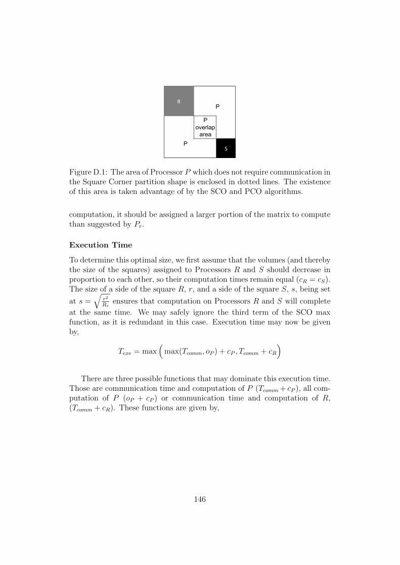
S
R
P overlap
area
P
P
Figure D.1: The area of Processor P which does not require communication inthe Square Corner partition shape is enclosed in dotted lines. The existenceof this area is taken advantage of by the SCO and PCO algorithms.
computation, it should be assigned a larger portion of the matrix to computethan suggested by Pr.
Execution Time
To determine this optimal size, we first assume that the volumes (and therebythe size of the squares) assigned to Processors R and S should decrease inproportion to each other, so their computation times remain equal (cR = cS).The size of a side of the square R, r, and a side of the square S, s, being set
at s =√
r2
Rrensures that computation on Processors R and S will complete
at the same time. We may safely ignore the third term of the SCO maxfunction, as it is redundant in this case. Execution time may now be givenby,
Texe = max(
max(Tcomm, oP ) + cP , Tcomm + cR
)There are three possible functions that may dominate this execution time.
Those are communication time and computation of P (Tcomm + cP ), all com-putation of P (oP + cP ) or communication time and computation of R,(Tcomm + cR). These functions are given by,
146
Texe(1)(Tcomm + cP ) = 2N2
(√Rr
T+
√1
T
)β+
2N
Sp
(Nr − r2 − r2√
Rr
+Nr√Rr
− r2
Rr
)Texe(2)(oP + cP ) =
N
Sp
(N2 − r2
Rr
− r2)
Texe(3)(Tcomm + cR) = 2N2
(√Rr
T+
√1
T
)β + r2
N
Sr
where SpN
is the number of elements computed per second by ProcessorP , and Sr
Nis the number of elements computed per second by Processor R.
In order to make the execution time equations easier to analyse, the con-stant factor N3β has been removed. This introduces a new variable c = Spβ,which represents a ratio between computation and communication speeds.The size of N and r have been normalised, so that r
Nbecomes r, and r is
understood to be 0 ≤ r < 1.
Texe(1)N3β
(Tcomm + cP ) =2
N
(√Rr
T+
√1
T
)+
2
c
(r − r2 − r2√
Rr
+r√Rr
− r2
Rr
)Texe(2)N3β
(oP + cP ) =(1− r2
Rr− r2)
c
Texe(3)N3β
(Tcomm + cR) =2
N
(√Rr
T+
√1
T
)+r2PrcRr
Lemma 1 (SCO Texe(1)). The completion time of the communication and thecomputation of the remainder of Processor P ’s elements will dominate themaximum function and determine the execution time of the Square Corner
partition shape for the SCO algorithm when T −Rr− 2cN
(√
Rr
T+√
1T
) + r(r+
2r−2√Rr
+ rRr− 2) < Pr <
2Rr
r− 2Rr − 2
√Rr + 2
√Rr
r− 2.
147
Proof. Directly compare each of the Texe functions, beginning with,
Texe(1) > Texe(2)
2
N
(√Rr
T+
√1
T
)+
2
c
(r − r2 − r2√
Rr
+r√Rr
− r2
Rr
)>
(1− r2
Rr− r2)
c
2c
N
(√Rr
T+
√1
T
)+ 2r − r2 − 2r2√
Rr
+2r√Rr
− r2
Rr
> 1
2c
N
(√Rr
T+
√1
T
)+ 2r − r2 − 2r2√
Rr
+2r√Rr
− r2
Rr
− T > 1− Pr −Rr − Sr
T −Rr −2c
N
(√Rr
T+
√1
T
)+ r(r +
2r − 2√Rr
+r
Rr
− 2)< Pr
And then comparing,
Texe(1) > Texe(3)
2
N
(√Rr
T+
√1
T
)+
2
c
(r − r2 − r2√
Rr
+r√Rr
− r2
Rr
)>
2
N
(√Rr
T+
√1
T
)+r2PrcRr
2
c
(r − r2 − r2√
Rr
+r√Rr
− r2
Rr
)>r2PrcRr
2Rr
r− 2Rr − 2
√Rr +
2√Rr
r− 2 > Pr
Lemma 2 (SCO Texe(2)). The computation of all elements assigned to Pro-cessor P will dominate the maximum function and determine the execu-tion time of the Square Corner partition shape for the SCO algorithm when
Pr < T − Rr − 2cN
(√
Rr
T+√
1T
) + r(r + 2r−2√Rr
+ rRr− 2) and when Pr <
Rr
r2− 1−Rr − 2cRr
r2N
(√Rr
T+√
1T
).
Proof. The comparison of Texe(1) and Texe(2) may be found in the proof ofLemma 1. The second comparison is given by,
Texe(2) > Texe(3)
(1− r2
Rr− r2)
c>
2
N
(√Rr
T+
√1
T
)+r2PrcRr
1− r2
Rr
− r2 − 2c
N
(√Rr
T+
√1
T
)>r2PrRr
Rr
r2− 1−Rr −
2cRr
r2N
(√Rr
T+
√1
T
)> Pr
148
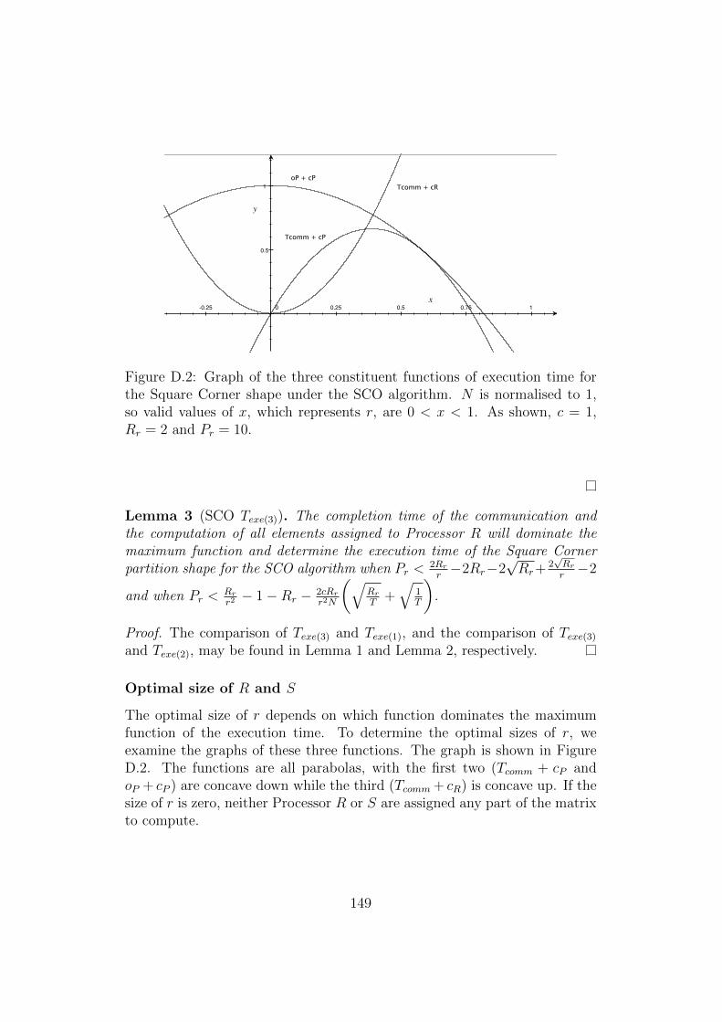
-0.25 0 0.25 0.5 0.75 1
0.5
1
Tcomm + cP
oP + cPTcomm + cR
Figure D.2: Graph of the three constituent functions of execution time forthe Square Corner shape under the SCO algorithm. N is normalised to 1,so valid values of x, which represents r, are 0 < x < 1. As shown, c = 1,Rr = 2 and Pr = 10.
Lemma 3 (SCO Texe(3)). The completion time of the communication andthe computation of all elements assigned to Processor R will dominate themaximum function and determine the execution time of the Square Cornerpartition shape for the SCO algorithm when Pr <
2Rr
r−2Rr−2
√Rr+
2√Rr
r−2
and when Pr <Rr
r2− 1−Rr − 2cRr
r2N
(√Rr
T+√
1T
).
Proof. The comparison of Texe(3) and Texe(1), and the comparison of Texe(3)and Texe(2), may be found in Lemma 1 and Lemma 2, respectively.
Optimal size of R and S
The optimal size of r depends on which function dominates the maximumfunction of the execution time. To determine the optimal sizes of r, weexamine the graphs of these three functions. The graph is shown in FigureD.2. The functions are all parabolas, with the first two (Tcomm + cP andoP + cP ) are concave down while the third (Tcomm + cR) is concave up. If thesize of r is zero, neither Processor R or S are assigned any part of the matrixto compute.
149
(1 ∩ 2) r =Rr +
√Rr −
√(2cRr
N)(1 +Rr + 2
√Rr)(
√Rr
T+√
1T
)
1 +Rr + 2√Rr
(D.1)
(2 ∩ 3) r =
√−( Pr
Rr+ 1 + 1
Rr)(2cN
√Rr
T+ 2c
N
√1T− 1)
( Pr
Rr+ 1 + 1
Rr)
(D.2)
(1 ∩ 3) r =2 + 2√
Rr
Pr
Rr+ 2√
Rr+ 2
Rr+ 2
(D.3)
D.1.2 SCO Optimal Shape
Theorem D.1.1 (SCO Square Corner). The Square Corner partition shapeminimizes execution time, i.e. is the optimum shape, when using the SCOMMM algorithm for computational ratios such that
Pr >2N(√
RrT
+√
1T)+ 2
c(r−r2− r2√
Rr+ r√
Rr− r2
Rr)− 2
N1Tc− 1
TN
and Pr >2cN
(√RrT+
√T )+2T (r−
r2− r2√Rr
+ r√Rr− r2
Rr)− Tc
N− 2c
N
√T , where r is the optimal size of the square
R, given in (D.3).
Proof. The Square Corner shape, as seen in graph 7.10, minimises executiontime along the highly heterogeneous processor ratios, intersecting with theBlock Rectangle and the Square Rectangle shape surfaces as the ratio ap-proaches Pr = Rr. To compare the Square Corner shape, we first determinewhich constituent function of the max will dominate the execution time atthose ratios. As heterogeneity decreases, and the intersections with SquareRectangle and Block Rectangle shapes are approached, it becomes increas-ingly vital to performance that powerful processors (R and S) not be leftidle. In these cases, for the ratios at which each function of the maximumintersects with these other shapes, by Lemma 1, the maximum function willbe dominated by the first function, Texe(1) = Tcomm + cP .
It is now possible to compare each shape directly.
150
SC < BR
2
N(
√Rr
T+
√1
T) +
2
c(r − r2 − r2√
Rr
+r√Rr
− r2
Rr
) <
2
N− PrTN
+ max
(PrTc,PrTc,PrTc
)2N
(√
Rr
T+√
1T
) + 2c(r − r2 − r2√
Rr+ r√
Rr− r2
Rr)− 2
N
1Tc− 1
TN
< Pr
SC < SR
2
N(
√Rr
T+
√1
T) +
2
c(r − r2 − r2√
Rr
+r√Rr
− r2
Rr
) <
1
N− 2
N
√1
T+ max
(PrTc,PrTc,PrTc
)2c
N(√RrT +
√T ) + 2T (r − r2 − r2√
Rr
+r√Rr
− r2
Rr
)− Tc
N− 2c
N
√T < Pr
Theorem D.1.2 (SCO Square Rectangle). The Square Rectangle partitionshape minimises execution time, i.e. is the optimum shape, when using theSCO MMM algorithm for computational ratios such that Pr < T − 2
√T and
Pr <2cN
(√RrT +
√T ) + 2T (r − r2 − r2√
Rr+ r√
Rr− r2
Rr)− Tc
N− 2c
N
√T
Proof. The ratios of intersection of the Square Rectangle and the SquareCorner shapes is found in the proof of Theorem 7.3.11 above. The comparisonof the Square Rectangle and Block Rectangles shapes gives,
SR < BR
1
N− 2
N
√1
T+ max
(PrTc,PrTc,PrTc
)<
2
N− PrTN
+ max
(PrTc,PrTc,PrTc
)1
N− 2
N
√1
T<
2
N− PrTN
Pr < T − 2√T
151
Corollary D.1.3 (SCO Block Rectangle). The Block Rectangle partitionshape minimises execution time, i.e. is the optimum shape, for all proces-sor computational power ratios except those specified in Theorems D.1.1 andD.1.2.
D.2 Parallel Communication with Overlap
In the Parallel Communication with Bulk Overlap (PCO) algorithm all datais sent among processors in parallel, while in parallel any elements that can becomputed without communication are computed. Once both communicationand overlapped computation are complete, the remainder of the computationbegins. The execution time for this algorithm is given by,
Texe = max(
max(Tcomm, oP )+cP ,max(Tcomm, oR)+cR,max(Tcomm, oS)+cS
)where Tcomm is the same as that of the PCB algorithm, oX is the num-
ber of seconds taken to compute any elements not requiring communication,by Processor X, and cX is the number of seconds taken to compute theremainder of the elements assigned to Processor X.
D.2.1 Square Corner
In the PCO algorithm, the Square Corner shape has a portion assigned toProcessor P , oP , which may be overlapped with the communication. Proces-sor P begins computation before Processors R and S, meaning that ProcessorP should be assigned more elements to compute. This will decrease the sizeof the squares assigned to Processor R and S, which we assert should bedecreased in proportion to each other such that cR = cS. In this section, wedetermine the optimal size of square assigned to Processors R and S. We fixthe size of the square of Processor S to be s = r√
Rr. The general form of the
execution time equation will then be,
Texe = max(
max(Tcomm, oP ) + cP , Tcomm + cR
)Execution Time
There exist three functions which may dominate the execution time functionfor this partition shape, Tcomm + cP , oP + cP , and Tcomm + cR. These aregiven by,
152
Texe(1)(Tcomm + cP ) = max(2rN − 2r2 + 2sN − 2s2, 2r2, 2s2)β
+2r(N − r) + 2s(N − r − s)
SpN
Texe(2)(oP + cP ) =N2 − r2 − s2
SpN
Texe(3)(Tcomm + cR) = max(2rN − 2r2 + 2sN − 2s2, 2r2, 2s2)β +r2
SrN
To simplify these equations, we substitute s, remove the constant N3βand normalize r
Nto r. As r and s are no longer independent variables,
the third term of Tcomm is redundant, and is ignored. The execution timefunctions may now be given by,
Texe(1)N3β
(Tcomm + cP ) =2
Nmax(r − r2 +
r√Rr
− r2
Rr
, r2)
+ 2r − r2 + r√
Rr− r2√
Rr− r2
Rr
c
Texe(2)N3β
(oP + cP ) =1− r2 − r2
Rr
c
Texe(3)N3β
(Tcomm + cR) =2
Nmax(r − r2 +
r√Rr
− r2
Rr
, r2) +r2PrcRr
Value of Tcomm
The Tcomm function may be dominated by either the communication time ofthe data sent by Processor P or the data sent by Processor R.
Theorem D.2.1 (PCO SC Tcomm). The Tcomm function of the Square Cornershape, under the PCO algorithm, will be dominated by the communicationtime of Processor P (the first term) when Pr < T − 1 +
√Rr− 2rRr− r, and
by the communication time of Processor R otherwise
153
Proof. Begin by stating,
VP > VR
r − r2 +r√Rr
− r2
Rr
> r2
1− r +1√Rr
− r
Rr
> r
Rr +√Rr > 2rRr + r
T +√Rr − 1 + r(2Rr + 1) < Pr
Optimal Size of R and S
The optimal size of r is found by examining the graphs of the constituentfunctions Texe(SC). The minimum will be found at the intersection of theconcave up and concave down parabolas, such that
r =−(2c
N+ 2c
N√Rr
) +√
(2cN
+ 2cN√Rr
)2 + 4( Pr
Rr− 2c
NRr− 2c
N+ 1
Rr+ 1)
2( Pr
Rr− 2c
NRr− 2c
N+ 1
Rr+ 1)
(D.4)
D.2.2 Square Rectangle
As with the SCO algorithm, the Square Rectangle shape does not have aportion which may be overlapped with communication under PCO. The timeof execution, as with PCB model, is given by,
Texe(SR)
N3β= max
( 1
N+
2
N√T− Rr
NT− Rr
NT√T− 3
NT,Rr
NT+
Rr
NT√T,
3
NT
)+ max
(PrTc,PrTc,PrTc
)Value of Tcomm
The Tcomm function may be dominated by the communication time of thedata sent by Processor P or S.
Theorem D.2.2 (PCO SR Tcomm). The Tcomm function of the RectangleCorner shape, under the PCO algorithm, will be dominated by the communi-cation time of Processor P (the first term) when Pr > 5 − 2
√T + Rr√
T, and
by the communication time of Processor S otherwise
154
Proof. First, the intersection of the equations of communication time forProcessors P and R lies at Pr = Rr+
2Rr√T−2√T+2. However, this intersection
may be show to lie outside the problem domain of Pr ≥ Rr. Instead, weconsider the intersection of Processor P and Processor S’s communicationtime. Begin by stating,
1
N+
2
N√T− Rr
NT− Rr
NT√T− 3
NT>
3
NT
Pr > 5− 2√T +
Rr√T
D.2.3 Block Rectangle
Texe(BR)
N3β= max
(PrNT
,2Rr
NT,
2
NT
)+ max
(PrTc,PrTc,PrTc
)Value of Tcomm
The Tcomm function may be dominated by either the communication time ofthe data sent by Processor P or the data sent by Processor R.
Theorem D.2.3 (PCO SC Tcomm). The Tcomm function of the Block Rectan-gle shape, under the PCO algorithm, will be dominated by the communicationtime of Processor P (the first term) when Pr > 2Rr, and by the communica-tion time of Processor R otherwise
Proof. The communication time of Processor R will always be equal to orlarger than the communication time of Processor S, 2Rr ≥ 2, as by definitionRr ≥ 1. Therefore, when communication of Processor P does not dominate,that of Processor R will.
D.2.4 PCO Optimal Shape
The optimal shape under the PCO algorithm depends on the value of c.When examining all three shapes to determine the optimal, we see that as cdecreases, all three equations converge. However, for larger values of c, theSquare Corner shape is optimal.
Theorem D.2.4 (PCO Square Rectangle). The Square Rectangle partitionshape minimises execution time, i.e. is the optimum shape, when using the
155
PCO MMM algorithm for computational ratios such that
Pr <1+ 2√
T−Rr
T− Rr
T√T− 3
T−2r2
N( r2
cRr− 1
Tc)
.
Proof. Examining the equations, we see that the Square Corner shape equa-tion is dominated by the communication and computation of R when theSquare Rectangle shape is dominated by the communication and computa-tion of P .
2
Nr2 +
r2PrcRr
<1
N+
2
N√T− Rr
NT− Rr
NT√T− 3
NT+PrTc
Pr <1 + 2√
T− Rr
T− Rr
T√T− 3
T− 2r2
N( r2
cRr− 1
Tc)
Corollary D.2.5 (PCO Square Corner). The Square Corner partition shapeminimises execution time, i.e. is the optimum shape, for all processor com-putational power ratios except those specified in TheoremD.2.4.
156
Bibliography
[1] T. G. Mattson, D. Scott, and S. Wheat, “A teraflop supercomputer in1996: the asci tflop system,” in Parallel Processing Symposium, 1996.,Proceedings of IPPS’96, The 10th International, pp. 84–93, IEEE, 1996.
[2] K. J. Barker, K. Davis, A. Hoisie, D. J. Kerbyson, M. Lang, S. Pakin,and J. C. Sancho, “Entering the petaflop era: the architecture and per-formance of roadrunner,” in Proceedings of the 2008 ACM/IEEE con-ference on Supercomputing, p. 1, IEEE Press, 2008.
[3] J. J. Dongarra, H. W. Meuer, and E. Strohmaier, “Top500 supercom-puter sites,” Supercomputer, vol. 13, pp. 89–111, 1997.
[4] H. W. Meuer, “The top500 project. looking back over 15 years of super-computing experience,” PIK-Praxis der Informationsverarbeitung undKommunikation, vol. 31, no. 2, pp. 122–132, 2008.
[5] E. Strohmaier, H. Simon, J. Dongarra, and M. Meuer, “Highlights ofthe 43rd top500 list.” http://www.top500.org/lists/2014/06/highlights/,June 2014.
[6] G. Shainer, T. Wilde, P. Lui, T. Liu, M. Kagan, M. Dubman, Y. Sha-har, R. Graham, P. Shamis, and S. Poole, “The co-design architecturefor exascale systems, a novel approach for scalable designs,” ComputerScience-Research and Development, vol. 28, no. 2-3, pp. 119–125, 2013.
[7] H. J. Siegel, L. Wang, V. P. Roychowdhury, and M. Tan, “Computingwith heterogeneous parallel machines: advantages and challenges,” inParallel Architectures, Algorithms, and Networks, 1996. Proceedings.,Second International Symposium on, pp. 368–374, IEEE, 1996.
[8] C. J. Thompson, S. Hahn, and M. Oskin, “Using modern graphics ar-chitectures for general-purpose computing: a framework and analysis,”in Proceedings of the 35th annual ACM/IEEE international symposiumon Microarchitecture, pp. 306–317, IEEE Computer Society Press, 2002.
157
[9] X. Xue, A. Cheryauka, and D. Tubbs, “Acceleration of fluoro-ct recon-struction for a mobile c-arm on gpu and fpga hardware: a simulationstudy,” in Medical Imaging, pp. 61424L–61424L, International Societyfor Optics and Photonics, 2006.
[10] V. W. Lee, C. Kim, J. Chhugani, M. Deisher, D. Kim, A. D. Nguyen,N. Satish, M. Smelyanskiy, S. Chennupaty, P. Hammarlund, et al., “De-bunking the 100x gpu vs. cpu myth: an evaluation of throughput com-puting on cpu and gpu,” in ACM SIGARCH Computer ArchitectureNews, vol. 38, pp. 451–460, ACM, 2010.
[11] F. Song and J. Dongarra, “A scalable approach to solving dense linearalgebra problems on hybrid cpu-gpu systems,” Concurrency and Com-putation: Practice and Experience, pp. 2–35, 2014.
[12] F. Tinetti, A. Quijano, A. De Giusti, and E. Luque, “Heterogeneous net-works of workstations and the parallel matrix multiplication,” in RecentAdvances in Parallel Virtual Machine and Message Passing Interface,pp. 296–303, Springer, 2001.
[13] J. Barbosa, J. Tavares, and A. J. Padilha, “Linear algebra algorithmsin a heterogeneous cluster of personal computers,” in HeterogeneousComputing Workshop, 2000.(HCW 2000) Proceedings. 9th, pp. 147–159,IEEE, 2000.
[14] Y. Wu, S. Hu, E. Borin, and C. Wang, “A hw/sw co-designed hetero-geneous multi-core virtual machine for energy-efficient general purposecomputing,” in Code Generation and Optimization (CGO), 2011 9thAnnual IEEE/ACM International Symposium on, pp. 236–245, IEEE,2011.
[15] C. Van Berkel, “Multi-core for mobile phones,” in Proceedings of theConference on Design, Automation and Test in Europe, pp. 1260–1265,European Design and Automation Association, 2009.
[16] R. Kumar, D. M. Tullsen, and N. P. Jouppi, “Core architecture opti-mization for heterogeneous chip multiprocessors,” in Proceedings of the15th international conference on Parallel architectures and compilationtechniques, pp. 23–32, ACM, 2006.
[17] A. R. Brodtkorb, C. Dyken, T. R. Hagen, J. M. Hjelmervik, and O. O.Storaasli, “State-of-the-art in heterogeneous computing,” Scientific Pro-gramming, vol. 18, no. 1, pp. 1–33, 2010.
158
[18] V. Boudet, F. Rastello, and Y. Robert, “Algorithmic issues for (dis-tributed) heterogeneous computing platforms,” in In Rajkumar Buyyaand Toni Cortes, editors, Cluster Computing Technologies, Environ-ments, and Applications (CC-TEA’99). CSREA, Citeseer, 1999.
[19] J.-N. Quintin, K. Hasanov, and A. Lastovetsky, “Hierarchical paral-lel matrix multiplication on large-scale distributed memory platforms,”in Parallel Processing (ICPP), 2013 42nd International Conference on,pp. 754–762, IEEE, 2013.
[20] D. Clarke, Z. Zhong, V. Rychkov, and A. Lastovetsky, “Fupermod: Aframework for optimal data partitioning for parallel scientific applica-tions on dedicated heterogeneous hpc platforms,” in Parallel ComputingTechnologies, pp. 182–196, Springer, 2013.
[21] L.-C. Canon, E. Jeannot, et al., “Wrekavoc: a tool for emulating het-erogeneity.,” in IPDPS, 2006.
[22] C. Augonnet, S. Thibault, R. Namyst, and P.-A. Wacrenier, “Starpu:a unified platform for task scheduling on heterogeneous multicore ar-chitectures,” Concurrency and Computation: Practice and Experience,vol. 23, no. 2, pp. 187–198, 2011.
[23] F. Song and J. Dongarra, “A scalable framework for heterogeneous gpu-based clusters,” in Proceedinbgs of the 24th ACM symposium on Paral-lelism in algorithms and architectures, pp. 91–100, ACM, 2012.
[24] A. Petitet, R. C. Whaley, J. Dongarra, and A. Cleary,HPL - A Portable Implementation of the High-performanceLinpack Benchmark For Distributed-memory Computers.http://www.netlib.org/benchmark/hpl/, 2008.
[25] L. S. Blackford, J. Choi, A. Cleary, E. D’Azevedo, J. Demmel, I. Dhillon,J. Dongarra, S. Hammarling, G. Henry, A. Petitet, et al., ScaLAPACKusers’ guide, vol. 4. siam, 1997.
[26] J. Dongarra and A. Lastovetsky, High performance heterogeneous com-puting, vol. 78. John Wiley & Sons, 2009.
[27] O. Beaumont, V. Boudet, A. Legrand, F. Rastello, and Y. Robert, “Het-erogeneity considered harmful to algorithm designers,” in 2000 IEEEInternational Conference on Cluster Computing (CLUSTER), pp. 403–403, IEEE Computer Society, 2000.
159
[28] O. Beaumont, V. Boudet, F. Rastello, and Y. Robert, “Matrix multipli-cation on heterogeneous platforms,” Parallel and Distributed Systems,IEEE Transactions on, vol. 12, no. 10, pp. 1033–1051, 2001.
[29] R. A. Van De Geijn and J. Watts, “Summa: Scalable universal matrixmultiplication algorithm,” Concurrency-Practice and Experience, vol. 9,no. 4, pp. 255–274, 1997.
[30] V. V. Williams, “Multiplying matrices faster than coppersmith-winograd,” in Proceedings of the forty-fourth annual ACM symposiumon Theory of computing, pp. 887–898, ACM, 2012.
[31] V. Strassen, “Gaussian elimination is not optimal,” Numerische Math-ematik, vol. 13, no. 4, pp. 354–356, 1969.
[32] B. Grayson and R. Van De Geijn, “A high performance parallel strassenimplementation,” Parallel Processing Letters, vol. 6, no. 01, pp. 3–12,1996.
[33] Y. Ohtaki, D. Takahashi, T. Boku, and M. Sato, “Parallel implemen-tation of strassen’s matrix multiplication algorithm for heterogeneousclusters,” in Parallel and Distributed Processing Symposium, 2004. Pro-ceedings. 18th International, p. 112, IEEE, 2004.
[34] G. Ballard, J. Demmel, O. Holtz, B. Lipshitz, and O. Schwartz,“Communication-optimal parallel algorithm for strassen’s matrix multi-plication,” in Proceedinbgs of the 24th ACM symposium on Parallelismin algorithms and architectures, pp. 193–204, ACM, 2012.
[35] G. Strang, “Introduction to linear algebra,” Cambridge Publication,2009.
[36] L. E. Cannon, “A cellular computer to implement the kalman filteralgorithm.,” tech. rep., DTIC Document, 1969.
[37] G. C. Fox, S. W. Otto, and A. J. Hey, “Matrix algorithms on a hypercubei: Matrix multiplication,” Parallel computing, vol. 4, no. 1, pp. 17–31,1987.
[38] R. C. Agarwal, S. M. Balle, F. G. Gustavson, M. Joshi, and P. Palkar,“A three-dimensional approach to parallel matrix multiplication,” IBMJournal of Research and Development, vol. 39, no. 5, pp. 575–582, 1995.
160
[39] E. Solomonik and J. Demmel, “Communication-optimal parallel 2.5 dmatrix multiplication and lu factorization algorithms,” in Euro-Par 2011Parallel Processing, pp. 90–109, Springer, 2011.
[40] D. Irony, S. Toledo, and A. Tiskin, “Communication lower bounds fordistributed-memory matrix multiplication,” Journal of Parallel and Dis-tributed Computing, vol. 64, no. 9, pp. 1017–1026, 2004.
[41] J. Choi, D. W. Walker, and J. J. Dongarra, “Pumma: Parallel uni-versal matrix multiplication algorithms on distributed memory concur-rent computers,” Concurrency: Practice and Experience, vol. 6, no. 7,pp. 543–570, 1994.
[42] M. Krishnan and J. Nieplocha, “Srumma: a matrix multiplication al-gorithm suitable for clusters and scalable shared memory systems,” inParallel and Distributed Processing Symposium, 2004. Proceedings. 18thInternational, p. 70, IEEE, 2004.
[43] O. Beaumont, V. Boudet, A. Legrand, F. Rastello, and Y. Robert, “Het-erogeneous matrix-matrix multiplication or partitioning a square intorectangles: Np-completeness and approximation algorithms,” in Par-allel and Distributed Processing, 2001. Proceedings. Ninth EuromicroWorkshop on, pp. 298–305, IEEE, 2001.
[44] A. L. Lastovetsky, “On grid-based matrix partitioning for heterogeneousprocessors.,” in ISPDC, pp. 383–390, 2007.
[45] O. Beaumont, V. Boudet, A. Petitet, F. Rastello, and Y. Robert, “Aproposal for a heterogeneous cluster scalapack (dense linear solvers),”Computers, IEEE Transactions on, vol. 50, no. 10, pp. 1052–1070, 2001.
[46] A. Kalinov and A. Lastovetsky, “Heterogeneous distribution of compu-tations solving linear algebra problems on networks of heterogeneouscomputers,” in High-Performance Computing and Networking, pp. 189–200, Springer, 1999.
[47] A. Kalinov and A. Lastovetsky, “Heterogeneous distribution of computa-tions solving linear algebra problems on networks of heterogeneous com-puters,” Journal of Parallel and Distributed Computing, vol. 61, no. 4,pp. 520–535, 2001.
[48] A. Lastovetsky and R. Reddy, “Data partitioning with a functional per-formance model of heterogeneous processors,” International Journal of
161
High Performance Computing Applications, vol. 21, no. 1, pp. 76–90,2007.
[49] D. Clarke, A. Lastovetsky, and V. Rychkov, “Column-based matrix par-titioning for parallel matrix multiplication on heterogeneous processorsbased on functional performance models,” in Euro-Par 2011: ParallelProcessing Workshops, pp. 450–459, Springer, 2012.
[50] D. Clarke, Design and Implementation of Parallel Algorithms for Mod-ern Heterogeneous Platforms Based on the Functional PerformanceModel. PhD thesis, University College Dublin, 2014.
[51] D. Clarke, A. Ilic, A. Lastovetsky, V. Rychkov, L. Sousa, and Z. Zhong,“Design and optimization of scientific applications for highly hetero-geneous and hierarchical hpc platforms using functional computationperformance models,” High-Performance Computing on Complex Envi-ronments, pp. 235–260, 2013.
[52] B. A. Becker and A. Lastovetsky, “Matrix multiplication on two inter-connected processors,” in Cluster Computing, 2006 IEEE InternationalConference on, pp. 1–9, IEEE, 2006.
[53] B. A. Becker and A. Lastovetsky, “Towards data partitioning for par-allel computing on three interconnected clusters,” in Parallel and Dis-tributed Computing, 2007. ISPDC’07. Sixth International Symposiumon, pp. 39–39, IEEE, 2007.
[54] B. A. Becker, High-level data partitioning for parallel computing on het-erogeneous hierarchical computational platforms. PhD thesis, UniversityCollege Dublin, 2010.
[55] Z. Zhong, V. Rychkov, and A. Lastovetsky, “Data partitioning on het-erogeneous multicore platforms,” in Cluster Computing (CLUSTER),2011 IEEE International Conference on, pp. 580–584, IEEE, 2011.
[56] Z. Zhong, V. Rychkov, and A. Lastovetsky, “Data partitioning onheterogeneous multicore and multi-gpu systems using functional per-formance models of data-parallel applications,” in Cluster Computing(CLUSTER), 2012 IEEE International Conference on, pp. 191–199,IEEE, 2012.
[57] A. DeFlumere, A. Lastovetsky, and B. A. Becker, “Partitioning for par-allel matrix-matrix multiplication with heterogeneous processors: Theoptimal solution,” in Parallel and Distributed Processing Symposium
162
Workshops & PhD Forum (IPDPSW), 2012 IEEE 26th International,pp. 125–139, IEEE, 2012.
[58] A. DeFlumere and A. Lastovetsky, “Optimal data partitioning shapefor matrix multiplication on three fully connected heterogeneous pro-cessors,” in Euro-Par 2014WS, HeteroPar 2014 - Twelfth InternationalWorkshop on Algorithms, Models and Tools for Parallel Computing onHeterogeneous Platforms, 2014, in press.
[59] R. W. Hockney, “The communication challenge for mpp: Intel paragonand meiko cs-2,” Parallel computing, vol. 20, no. 3, pp. 389–398, 1994.
[60] A. Lastovetsky and R. Reddy, “Data partitioning for multiprocessorswith memory heterogeneity and memory constraints,” Scientific Pro-gramming, vol. 13, no. 2, pp. 93–112, 2005.
[61] R. C. Whaley and J. J. Dongarra, “Automatically tuned linear algebrasoftware,” in Proceedings of the 1998 ACM/IEEE conference on Super-computing, pp. 1–27, IEEE Computer Society, 1998.
[62] A. Marletta, “Cpulimit.” https://github.com/opsengine/cpulimit, 2012.
[63] A. DeFlumere and A. Lastovetsky, “Searching for the optimal data parti-tioning shape for parallel matrix matrix multiplication on 3 heterogenousprocessors,” in Parallel and Distributed Processing Symposium Work-shops & PhD Forum (IPDPSW), 2014 IEEE 28th International, IEEEComputer Society, 2014.
[64] D. S. Johnson, C. H. Papadimitriou, and M. Yannakakis, “How easy islocal search?,” Journal of computer and system sciences, vol. 37, no. 1,pp. 79–100, 1988.
[65] S. Kirkpatrick, C. D. Gelatt, M. P. Vecchi, et al., “Optimization bysimmulated annealing,” science, vol. 220, no. 4598, pp. 671–680, 1983.
[66] J. Choi, J. J. Dongarra, L. S. Ostrouchov, A. P. Petitet, D. W. Walker,and R. C. Whaley, “Design and implementation of the scalapack lu,qr, and cholesky factorization routines,” Scientific Programming, vol. 5,no. 3, pp. 173–184, 1996.
[67] A. Buttari, J. Langou, J. Kurzak, and J. Dongarra, “A class of paral-lel tiled linear algebra algorithms for multicore architectures,” ParallelComputing, vol. 35, no. 1, pp. 38–53, 2009.
163
[68] J. Choi, J. Dongarra, S. Ostrouchov, A. Petitet, D. Walker, and R. C.Whaley, “A proposal for a set of parallel basic linear algebra subpro-grams,” in Applied Parallel Computing Computations in Physics, Chem-istry and Engineering Science, pp. 107–114, Springer, 1996.
[69] J. Barbosa, C. Morais, and A. J. Padilha, “Simulation of data distri-bution strategies for lu factorization on heterogeneous machines,” inParallel and Distributed Processing Symposium, 2003. Proceedings. In-ternational, pp. 8–pp, IEEE, 2003.
[70] P. Boulet, J. Dongarra, F. Rastello, Y. Robert, and F. Vivien, “Algorith-mic issues on heterogeneous computing platforms,” Parallel processingletters, vol. 9, no. 02, pp. 197–213, 1999.
[71] A. Lastovetsky and R. Reddy, “A novel algorithm of optimal matrix par-titioning for parallel dense factorization on heterogeneous processors,”in Parallel Computing Technologies, pp. 261–275, Springer, 2007.
[72] A. Lastovetsky and R. Reddy, “Data distribution for dense factorizationon computers with memory heterogeneity,” Parallel Computing, vol. 33,no. 12, pp. 757–779, 2007.
[73] O. Beaumont, A. Legrand, Y. Robert, et al., “Data allocation strategiesfor dense linear algebra on two-dimensional grids with heterogeneouscommunication links,” Tech. Rep. 4165, INRIA, 2001.
[74] A. DeFlumere and A. Lastovetsky, “Theoretical results on optimal par-titioning for matrix-matrix multiplication with two processors,” Tech.Rep. UCD-CSI-2011-09, School of Computer Science and Informatics,University College Dublin, 2011.
[75] A. DeFlumere and A. Lastovetsky, “Theoretical results for data parti-tioning for parallel matrix multiplication on three fully connected hetero-geneous processors,” Tech. Rep. UCD-CSI-2014-01, School of ComputerScience and Informatics, University College Dublin, 2014.
164
Related Documents


