Working Paper Series
Why Are the Inventory Estimates of Shoppers So Biased?
Reference, Size, and Salience Biases in Household Inventory Estimations
by
Pierre Chandon
and
Brian Wansink
2005/77/MKT
(Revised version of 2005/47/MKT)
Faculty & Research

1
Why Are the Inventory Estimates of Shoppers So Biased?
Reference, Size, and Salience Biases in Household Inventory Estimations
Pierre Chandon
INSEAD
Brian Wansink* Cornell
December 12, 2005
Under Second-Round Review at Journal of Marketing * Pierre Chandon is Assistant Professor of Marketing at INSEAD, Boulevard de Constance,
77300 Fontainebleau, France; +33 1 60 72 49 87 (phone), +33 1 60 74 61 84 (fax),
[email protected]. Brian Wansink is the John S. Dyson Chair of Applied Economics
and Management, of Marketing, and of Nutritional Science at Cornell University, 110 Warren
Hall, Ithaca, NY 14853-7801; [email protected].

2
Why Are the Inventory Estimates of Shoppers So Biased?
Reference, Size, and Salience Biases in Household Inventory Estimations
Abstract
Biases in estimating the level of product inventory in one’s household can lead to
overstocking and waste or to stockouts and unfulfilled demand. To understand the origin of
these biases, the authors develop a psychophysical model of inventory estimation. This model
argues that consumers anchor their estimations on their average inventory and that
adjustments from the anchor follow an inelastic power function, leading to overestimations of
low levels of inventory and underestimations of high levels. Two laboratory experiments and
two field studies involving 29 product categories confirm this, and show that inventory
estimates are less accurate for product categories that are bought on impulse, difficult to
stockpile, and that have a low promotional elasticity. Importantly, the results also show that it
is inventory estimates—not actual inventory levels—that drive subsequent purchase
incidence. In a final simulation, the authors examine the implications for consumers (in terms
of waste and unfulfilled demand) and for retailers (in terms of promotion targeting) of their
finding that inventory estimations biases are driven by perceptual factors and not fear of
overstocking or of stockouts.

3
“I buy lots of things and then go back to the house and see the fridge is full of all the stuff I’ve just bought.”
—Prince William, Heir of the British Throne, (BBC News 2003).
Biases in inventory estimations can lead to overstocking and stockout in one’s household.
Overstocking contributes to households wasting an estimated 14% of their meat, grain, fruit,
and vegetables purchases (Jones et al. 2003). Stockouts contribute to unfulfilled demand,
which represents a wasted opportunity for consumers as well as for retailers and
manufacturers. For example, the success of the “Got Milk?” advertising campaign is primarily
attributed to the fact that it reduced the frequency of milk stockouts in consumers’
refrigerators (Manning 1999). Improving our understanding of why consumers’ inventory
estimations are so biased that they lead to seemingly unavoidable reoccurrences of
overstocking and stockouts is important for the welfare of budget-pressured and time-
pressured consumers.
Understanding consumers’ inventory biases is also an important issue for managers and
researchers because these biases influence stockpiling, consumption, and repurchase
decisions, and therefore affect promotional elasticity (Ailawadi and Neslin 1998; Chandon
and Wansink 2002; Meyer and Assunçao 1990; Neslin and Schneider 1996; Sun 2005).
Importantly, biased inventory estimations also imply that the models and policy
recommendations of purchase and consumption models may be biased, since these models
typically assume that consumers know how much of the product is in their pantry. For
example, biased inventory estimations may explain why the primary demand portion of
integrated choice, quantity, and incidence models “typically generates the least reliable
parameter estimates and the poorest model fits” (Bell, Chiang, and Padmanabhan 1999, p.
513).
A recent surge of interest in estimation biases underscores the importance of understanding
consumers’ inventory estimation biases. Researchers have shown that reference levels,

4
stimulus size, and salience influence consumers’ estimations of product volume (Krider,
Raghubir, and Krishna 2001; Raghubir and Greenleaf 2005; Raghubir and Krishna 1999),
numerosity (Krishna and Raghubir 1997; Pelham, Sumarta, and Myaskovsky 1994), as well
estimations of purchase or consumption frequency and duration (Collopy 1996; Lee, Hu, and
Toh 2000; Menon, Raghubir, and Schwarz 1995; Nunes 2000). Still, no research has directly
examined whether household inventory estimations are accurate and whether they are biased
by the reference inventory, by inventory size, and by inventory salience.
This research addresses four unanswered questions regarding consumers’ inventory
estimations that are of interest to consumers, marketers, and researchers: 1) How do
consumers estimate how much of the product they have in inventory? 2) How accurate are
these estimations? 3) Do inventory estimations predict purchase incidence better than actual
inventory? 4) What is the relationship between inventory estimation biases and key category
characteristics, such as the degree of impulse buying, the ease of stockpiling, and the average
promotional elasticity?
To answer these questions, we build upon psychophysics research on magnitude estimation
and develop a model of consumer inventory estimates which incorporates reference, size, and
salience effects. We then test the predictions of the model in two laboratory experiments, in
which we manipulate internal and external reference levels, the actual size of the inventory,
and its salience. We further test the model in two field studies involving 29 product
categories. These studies demonstrate the robustness of the model predictions, they show that
estimated inventory levels predict repurchase decisions better than actual inventory levels do,
and that inventory estimation biases are related to key category characteristics. In the general
discussion, we show how this model can account for seemingly inconclusive findings in other
quantity estimation tasks, and we then outline the implications for consumers, researchers,

5
and marketers of our finding that inventory estimations are not influenced by fear of
overstocking or of stockouts, but are driven by perceptual biases.
A MODEL OF CONSUMERS’ INVENTORY ESTIMATIONS
Building on psychophysical research on magnitude estimations and spatial judgments, we
build a model of how consumers estimate the quantity of a product that they have in
inventory, and we show how its predictions can be tested. The key features of the model are:
(1) that consumers anchor their estimations on internal or external reference levels and
insufficiently adjust for the actual inventory level, (2) that the adjustment is inelastic (it
increases more slowly than the true deviation from the reference level, and hence its quality
worsens as the deviation increases), and (3) that the adjustment is more elastic (and accurate)
when inventory is perceptually salient. We now show how each prediction can be derived
from the literature.
Reference Effects
Inventory estimations either involve judgments of numerosity (such as “How many eggs do
I have left?”) or judgments of volume (such as “How many ounces of coffee do I have left?”).
Many studies have shown that consumers anchor numerosity and volume estimations on
salient internal or external reference levels and fail to adjust sufficiently for deviations from
the reference level. For example, Krishna and Raghubir (1997) showed that consumers’
estimation of the number of dots in a line is higher when the dots are in multiple clusters (high
reference anchor condition) than when they are all together in one uninterrupted line (low
reference anchor condition). Raghubir and Krishna (1999) and Wansink and Van Ittersum
(2003) showed that volume estimations are anchored on the elongation of the container.
Finally, Krider, Raghubir, and Krishna (2001) showed that consumers anchor area estimations
on the most salient dimension, where salience is context dependent. For example, they

6
showed that the orientation of a square influences whether the diagonal or a side is used as an
anchor when estimating its surface (see also Pelham, Sumarta, and Myaskovsky 1994).
In the context of inventory estimations, we expect that the default anchor is the average
category inventory level for each consumer. This is a reasonable assumption because in the
absence of other information on actual inventory, the average inventory level is the best
estimator of actual inventory if inventory follows a normal or a uniform distribution.
However, consistent with Krider, Raghubir, and Krishna’s (2001) results, we expect that
consumers will use external anchors if they are made contextually salient (for example, by
asking consumers to explicitly judge whether an inventory level is above or below some
number). In summary, we expect that consumers anchor their inventory estimations on their
average inventory, except when external reference levels are made salient (in which case,
these reference levels serve as anchors).
Size Effects
Recent research on anchoring effects has shown that, once individuals have selected a
reference as an anchor, they insufficiently adjust for the difference between the reference and
the actual value of the magnitude to be estimated (Epley and Gilovich 2001). For example,
Epley and Gilovich (2004) showed that people estimate the number of days taken by Mars or
Neptune to orbit the sun by using the number of days taken by the Earth as an anchor (365
days). As a result, they adjust more for Neptune (mean estimated answer is 3,447 days) than
for Mars (mean estimated answer is 574 days) because they know that Neptune is further
away from the Sun than Mars, but they still fall short of the truth (60,225 days for Neptune
and 869 days for Mars).
Our model contributes to the research on anchoring and adjustment by further predicting
that the adjustment is inelastic to actual deviations in inventory size, with adjustment to actual
size following a compressive power function (i.e., EST = a*(ACT)b, where b < 1, EST is the

7
estimated inventory, and ACT is the actual inventory). The inelasticity of adjustment is
caused by the well-known “size effect,” which is that the percentage change in estimations is
lower than the percentage change in actual inventory size (Stevens 1986; Teghtsoonian 1965).
As a result, adjustments become less effective as the deviation between the reference level and
the actual inventory level increases.
As reviewed by Krueger (1989), there is considerable evidence that magnitude estimations
follow a compressive power function of actual magnitudes. For example, Teghtsoonian
(1965) found that the exponent of the power function is about 0.7 when estimating three-
dimensional objects. Frayman and Dawson (1981) examined exponents of power functions for
different shapes (cubes, spheres, octahedrons, cylinders, tetrahedrons), and found that they
were all around 0.6. For perceived numerosity judgments, Krueger (1984; 1982) found a
power exponent between .80 and .82. Overall, there is strong support in the literature for our
prediction that not only do consumers fail to adjust sufficiently for the deviation from the
reference level, but that such adjustments are inelastic and therefore increase at a lower rate
than the true difference between the reference level and the actual inventory level.
Salience Effects
It is a known fact that the power exponent, which measures the elasticity of estimations to
actual changes in the magnitude of the stimuli, is influenced by the perceptual salience of the
different dimensions of the stimulus. For example, Krider, Raghubir and Krishna (2001)
found that the power exponent of area estimations for two-dimensional objects is greater
when the salience of secondary dimensions (those which are not used as anchors) is increased.
For example, because people anchor area estimations of circles on the length of their
horizontal diameters, area estimations and willingness to pay for round pizzas are more
sensitive to the actual size of the circle when the vertical diameter is made salient. More
8
generally, many studies have found that the salience of a physical magnitude is positively
correlated with the accuracy of its estimations (Kang, Herr, and Page 2003).
Building on these results, we predict that the elasticity of adjustment improves with the
perceptual salience of the product in inventory (and hence that the power exponent is greater
when inventory is salient than when it is not). Following Krider, Raghubir, and Krishna
(2001), we define salience as the ability of the product’s inventory to attract attention. For
example, the salience of a product’s inventory increases if the product is stored in a visible
place or if it is purchased or consumed frequently, because these factors increase attention to
the actual inventory level. When inventory is salient, consumers are more likely to know
whether the reference level that they anchor on is wrong and should be adjusted. In the
extreme case, consumers may have encoded salient inventory so well that they do not need to
rely on the reference level at all. When inventory is not salient, however, consumers may not
even know whether actual inventory is above or below the reference level, and will therefore
rely mostly on the reference anchor. We therefore expect that inventory estimations are
adjusted slightly when inventory is not salient and are adjusted more strongly when inventory
is salient. In other words, we expect that inventory estimations are more sensitive to actual
inventory—and thus more accurate—when inventory is salient than when it is not.
Modeling Reference, Size, and Salience Effects
We now provide an overview of how we test whether inventory estimations are influenced
by internal and external reference levels, the actual size of the inventory, and its salience. At
its core, our method consists of estimating a series of power models in different conditions
(e.g., when salience is low or high, when anchors are low or high). The power models are as
follows:
(1) EST = a*(ACT)b,

9
where EST is estimated inventory, ACT is actual inventory, and a and b are parameters
estimated via regression.
We use power models because they are consistent with psychophysical research on
magnitude estimation and because of their many desirable properties. First, the model
intercept (a) captures systematic differences between estimated and actual inventory,
regardless of inventory level. Changes in the intercepts shift the power curve up or down but
leave the shape of the curve unchanged. We can therefore test our prediction that internal or
external anchors shift estimations toward the reference level by examining the value of the
intercept (a) across anchor conditions. Second, the power exponent (b) measures the elasticity
of estimations and influences the shape of the power curve. If b = 1, estimations increase at
the same rate as actual inventory. If b < 1, the power function is compressive and estimations
are inelastic (i.e., the percentage change in estimations is lower than the percentage change in
actual inventory or, stated differently, estimations increase at a slower rate than actual
inventory. For example, if b = .5 and actual inventory increases by 50% (i.e., by a factor of
1.5), estimations increase by a factor of (1.5).5 = 1.225 (i.e., 22.5%). If b > 1, the power
function is expansive, estimations are elastic (they increases at a faster rate than actual
inventory). We can therefore test our prediction that inventory estimations are inelastic by
verifying that b is lower than 1. Third, we can use the power model to compute the crossover
inventory level at which estimations are accurate (ACT* = a1/(1-b)). Inventory levels below
ACT* tend to be overestimated and inventory levels above ACT* tend to be underestimated.
We can then compare ACT* with the hypothesized reference level (e.g., the individual’s
average inventory). Fourth, the power function treats positive and negative deviations from
the crossover level similarly (i.e., the power exponent is the same, regardless of inventory
level: there is no asymmetry between “gains” and “losses”). Note however, that the symmetry
in the power model leads to asymmetry when using conventional measures of accuracy, such

10
as absolute error (|estimated – actual|) or percentage absolute error (|estimated –actual|/actual).
In fact, a positive deviation from the crossover inventory level always leads to a smaller
percentage absolute error (but to a larger absolute error) than a similar-size negative deviation
from the crossover inventory level.1
To test the hypothesized reference and salience effects, we estimate a different power
model for each reference and salience condition. We illustrate how salience effects can be
incorporated, but the approach is exactly the same when examining the effects of reference
levels:
(2) EST = a*(ACT)b when salience is low,
EST = a’*(ACT)b’ when salience is high.
To facilitate the statistical estimation of these power models, we linearized them as
follows:2
(3) ln(EST) = ln(a) + b*ln(ACT), when salience is low,
ln(EST) = ln(a’) + b’*ln(ACT), when salience is high.
In order to test whether a is statistically different from a’ and whether b is statistically
different from b’, we estimate the following moderated regression:
(4) ln(EST) = α + β*SAL + δ*ln(ACT) + γ*ln(ACT)*SAL + ε,
where SAL is a binary variable coded as –½ when salience is low and as ½ when salience is
high, ε is the error term, and α, β, δ, and γ are estimated via OLS. These parameters are
1 For example, if EST = 3*ACT.5, ACT* = 9 units. The absolute error (AE) and percentage absolute error (PAE) when inventory is above the crossover level by 6 units (ACT = 15 units) are: AE = 3.38 units and PAE = 23%. When inventory is below the crossover level by 6 units (ACT = 3 units), AE = 2.2 units and PAE = 73%. 2 The linearization prevents the model from being estimated when either EST or ACT is zero. To overcome this limitation, it is possible to estimate the following nonlinear model with the Levenberg-
Marquardt least-square algorithm: EST = α* βSAL*(ACT)δ*(γ)SAL, where α = (a*a’)½ is the geometric mean of the intercepts across the low and high salience conditions; β = a’/a measures the ratio of two intercepts; δ = (b*b’)½ is the geometric mean of the power exponent across the low and high salience conditions and γ = b’/b is the ratio of the two power exponents. In all our analyses, both methods provide very similar estimates, and we therefore use the Levenberg-Marquardt least-square
11
interpreted as follows: α is a measure of the average intercept across the two salience
conditions (eα = (a*a’)½ and is therefore the geometric mean of the two intercepts), β
measures the main effect of salience on the intercepts (eβ = a’/a), δ is a measure of the average
power exponent across the two salience conditions (δ = (b + b’)/2), and γ measures the effects
of salience on the power exponent, that is, the interaction between salience and actual
inventory (γ = b’– b). If, as predicted, salience improves the accuracy of estimations by
reducing the degree of compression, we would expect γ to be positive and statistically
different from 0. We use this general method to simultaneously test for reference, size, and
salience effects in inventory estimations in two laboratory experiments and two field studies.
EXPERIMENT 1: HOW INVENTORY SIZE AND EXTERNAL ANCHORS
INFLUENCE INVENTORY ESTIMATIONS
Procedure
The objective of Experiment 1 is to test how external anchors and inventory size influence
inventory estimations (the effects of internal anchors and of inventory salience are tested in
Experiment 2). To achieve this objective, Experiment 1 used a mixed design with one within-
subject factor with four levels (1, 3, 7, or 9 units in inventory), one between-subject factor
with three levels (no external anchor, low external anchor, or high external anchor) and two
replications (two different products) for each level of inventory.
Participants first examined a color picture of a pantry containing eight target products and
thirteen other products in different quantities. The pantry contained one unit of two target
products, three units of two other target products, seven units of two other target products, and
nine units of the last two target products. In each picture, the mean inventory level across the
twenty-one target products was four units. Participants were later asked to recall the inventory
level of the eight target products (Coca-Cola cans, Lifesavers candy, Smucker’s jam,
algorithm only when the number of observations is small enough to make incorporating zeroes desirable.

12
Campbell’s soup, Charmin toilet tissue, Crest toothpaste, Carr’s crackers, and Heinz tomato
sauce). The products were rotated across the four inventory level conditions following a
Latin-square design. The inventory levels of the target products were selected based on a pre-
study indicating that this range (1 to 9) would straddle the average inventory of these products
for almost all respondents (the typical average inventory for these products is 3 or 4 units).
The participants were 216 undergraduate students who had been awarded extra credit
participation points for a course they were attending. They were told that the aim of the study
was to measure their liking of different types of teas. Consistent with this, we first asked them
to evaluate the three brands of tea that were present in the pantry. To direct their attention
toward the other products in the pantry (including the eight target products), we asked the
participants to estimate the overall quality of the brands displayed and to indicate whether
some of these products should be stored in a refrigerator rather than in a pantry. We then
asked each participant to return the first booklet containing the pantry picture. After a brief
distracter task, we gave them a second booklet containing a typical anchoring manipulation.
Participants in the high external anchor condition (low external anchor condition) were asked
to indicate whether the number of units of each of the eight target products was above or
below nine (one). They were then asked to estimate the number of units of the target products.
Participants in the control condition were simply asked to estimate the number of units of the
target products. Finally, all the participants were asked to write down how they had estimated
the inventory levels for these products.
Results
Consider first the estimations made in the control (no external anchor) condition. Figure 1
shows that the mean estimated inventory was well below reality when there were 7 or 9 units
in inventory, close to reality when there were 3 products in inventory, and slightly above
13
reality when only 1 product was in inventory. To formally test size effects in the control
condition, we estimated the following linear regression via OLS:
(5) ln(ESTij) = ln(a) + b*ln(ACTij) + ∑cj*CATj + ε,
where ESTij is the estimated inventory of product j by participant i, ACTij is the actual
inventory, CATj are seven binary variables accounting for product differences (j = {1, … 7}),
and ε is the error term.
--- Insert Figure1 about here ---
As expected, the power exponent was statistically below 1 (b = .43, t-test of difference
from 1 = –9.1, p < .001) and the intercept was statistically above 0 (ln(a) = .58, t = 11.8, p <
.001), which indicates that the intercept of the power model (a = 1.79) is statistically larger
than 1. Five of the seven product-specific intercepts were statistically significant. In addition,
we compared the fit of the power model with that of an alternative linear model (ESTij = a +
b* ACTij + ∑cj*CATj + ε). As expected, the R² was stronger for the power model (R² = .36)
than for the linear model (R² = .33) and the mean average percentage error was lower for the
power model (MAPE = .58) than for the linear model (MAPE = .74, paired t-test = 21.3, p <
.001). All these results show that, as predicted, consumer inventory estimations in the control
condition follow a compressive power function of actual inventory.
We now turn to the analysis of the anchoring manipulation. As a manipulation check, we
asked two coders, unaware of the objective of the experiment, to classify consumers’
retrospective protocols into three categories. Protocols mentioning how much participants
usually had of the product in their own inventory or how much they normally consumed of
these products were classified in the “internal anchor” category. Protocols mentioning
recalling the picture of the pantry or the space and shape of the pile of products in that picture
were classified in a “visual memory” category. Other statements, such as “I just guessed”,
were classified in an “other” category. Consistent with the anchoring literature, which shows

14
that people are unaware of the effects of external anchors (Mussweiler, Strack, and Pfeiffer
2000), no protocol mentioned the anchoring manipulation. An analysis of the 166 useable
protocols shows that the frequency of protocols mentioning internal anchors was higher in the
control condition (M = 22.1%) than in the two external anchor conditions (M = 7.1%, χ² = 7.8,
p < .01). This suggests that, as predicted in the model, consumers use internal anchors in the
control condition and external anchors when they are made contextually salient.
Figure 1 shows that the anchoring manipulation systematically shifted inventory
estimations toward the anchor but did not influence the relationship between estimated and
actual inventory (the power curves are parallel). To formally test anchoring effects, we
estimated the following regression:
(6) ln(ESTij) = α + β*ln(ACTij) + δ*EXTANCH1i + γ*EXTANCH9i
+ λ*EXTANCH1i*ln(ACTij) + θ* EXTANCH9i*ln(ACTij) + ∑cj*CATj + εij,
where ESTij is the estimated inventory for product j by participant i, ACTij is the (geometric)
mean-centered3 actual inventory for product j and participant i, EXTANCH1i is a binary
variable taking the value of ⅔ if participant i was in the low external anchor condition (anchor
= 1) and –⅓ otherwise, EXTANCH9i is a binary variable taking the value of ⅔ if participant i
was in the high external anchor condition (anchor = 9) and –⅓ otherwise, and CATj are seven
binary variables accounting for product differences (j = {1, … 7}). The simple effects of both
external anchors were statistically significant and in the expected direction (δ = –.07, t = –2.0,
p < .05 for the anchor on 1 unit and γ = .27, t = 7.8, p < .01 for the anchor on 9 units),
indicating that inventory estimations were assimilated toward the anchors. Consistent with the
model, the interaction parameters were not statistically significant (λ = .03, t = .6, p = .52 and
3 In practice, we divide actual inventory by its mean across inventory conditions (5 units). In a moderated regression, mean-centering the variables involved in an interaction allows us to estimate the main effects of the variables involved in an interaction when the other variables involved in the interaction are at their mean. For example, it allows us to estimate the effects of anchoring on inventory estimations when inventory level is at its average level (5 units). We use geometric mean-
15
θ = .2, t =.4, p = .68), indicating that the degree of compression of inventory estimations was
the same across the three conditions. Finally, the intercept was statistically different from 0, (α
= 1.21, t = 78, p < .01), indicating significant overestimation when actual inventory was one
unit (in the control condition) and four of the product-specific intercepts were statistically
significant.
Discussion
Experiment 1 shows that consumers’ inventory estimations are assimilated toward external
anchors and are adjusted for the actual inventory level through a nonlinear compressive power
function. Experiment 1 also shows that the rate of adjustment for the actual size of the
inventory remains constant, regardless of which reference levels serve as anchors. In other
words, external anchors do not influence the exponent of the power function, and hence do
not influence the quality of adjustments from the reference level. Finally, the protocols
provide indirect evidence that consumers rely on internal anchors when external anchors are
not salient. However, because we did not measure the value of these internal anchors, we
cannot test the effects of internal anchors or determine whether an average home inventory
can serve as one. Experiment 2 further tests the model by examining the effects of internal
anchors and by directly manipulating product salience.
EXPERIMENT 2: HOW INTERNAL ANCHORS, INVENTORY SALIENCE, AND
INVENTORY SIZE INFLUENCE INVENTORY ESTIMATIONS
Procedure
Experiment 2 used the same procedure and stimuli as Experiment 1, but with three
important differences. First, we did not manipulate external anchors but asked each participant
to indicate the average inventory of the eight target products in their own house (the
hypothesized internal anchor). Second, we manipulated the perceptual salience of the target
centering rather than arithmetic mean centering to be consistent with the power functional form and to prevent negative values whose logs cannot be computed.
16
products in three combined ways. Salient products were located on the top or middle shelf of
the pantry (as opposed to the bottom shelf), separate from other products (rather than being
crowded together with them), and were given multiple facings when available in more than
one unit (rather than being stacked together in an overlapping fashion). Each of the eight
target products was assigned to one of the eight conditions created by the two (high or low
salience) by four (1, 3, 7 or 9 units) design. As in Experiment 1, the products were rotated
across the eight inventory size and salience conditions following a Latin-square design. The
third difference was that we asked participants to rate how visible each product was in the
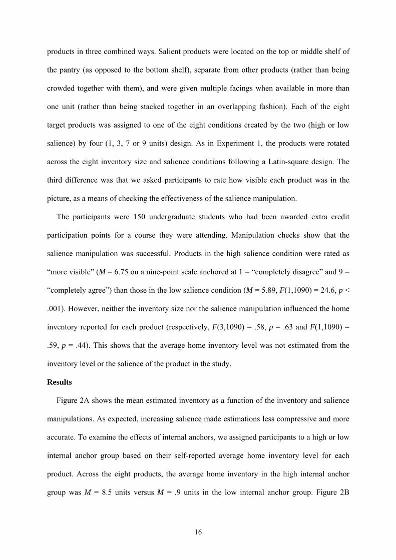
picture, as a means of checking the effectiveness of the salience manipulation.
The participants were 150 undergraduate students who had been awarded extra credit
participation points for a course they were attending. Manipulation checks show that the
salience manipulation was successful. Products in the high salience condition were rated as
“more visible” (M = 6.75 on a nine-point scale anchored at 1 = “completely disagree” and 9 =
“completely agree”) than those in the low salience condition (M = 5.89, F(1,1090) = 24.6, p <
.001). However, neither the inventory size nor the salience manipulation influenced the home
inventory reported for each product (respectively, F(3,1090) = .58, p = .63 and F(1,1090) =
.59, p = .44). This shows that the average home inventory level was not estimated from the
inventory level or the salience of the product in the study.
Results
Figure 2A shows the mean estimated inventory as a function of the inventory and salience
manipulations. As expected, increasing salience made estimations less compressive and more
accurate. To examine the effects of internal anchors, we assigned participants to a high or low
internal anchor group based on their self-reported average home inventory level for each
product. Across the eight products, the average home inventory in the high internal anchor
group was M = 8.5 units versus M = .9 units in the low internal anchor group. Figure 2B

17
shows mean estimated inventory as a function of actual inventory for both internal anchor
groups. As expected, estimations in the high internal anchor condition were higher than those
in the low internal anchor condition, regardless of inventory level, but the two estimation
curves remained parallel, suggesting that internal anchors (unlike the salience manipulation)
did not influence the elasticity of adjustments.
--- Insert Figure 2 about here ---
To directly test our predictions that salience reduces the degree of compression of
inventory estimations and that inventory estimations shift toward internal reference levels, we
estimated the following regression:
(7) ln(ESTij) = α + β*ln(ACTij) + δ*INTANCHij + γ*SALij
+ λ*INTANCHij*ln(ACTij) + θ*SALij*ln(ACTij) + ∑cj*CATj + εij,
where ESTij is the estimated inventory for product j by participant i, ACTij is the geometric
mean-centered actual inventory for product j and participant i, INTANCHij is a binary
variable taking the value of ½ if the home inventory of participant i for product j is in the top
50% of the distribution for this product and –½ otherwise, SALij is a binary variable taking
the value of ½ if product j is in the high salience condition for participant i and –½ otherwise,
and CATj are seven binary variables accounting for product differences (j = {1, … 7}).
As in Experiment 1, the power exponent was statistically below 1 (β = .41, t-test of
difference from 1 = –28.9, p < .001), indicating that the rate of adjustment increases more
slowly than the actual inventory size. The coefficient capturing the simple effect of the
internal anchor was positive and statistically significant (δ = .09, t = 2.3, p < .05), and its
interaction with the actual inventory level was not statistically significant (λ = .02, t = .5, p =
.61). This shows that inventory estimations were assimilated toward the average home
inventory for that product, but that this internal anchor did not change the rate at which
estimations were adjusted for the actual inventory level. The main effect of the salience

18
manipulation was positive and statistically significant (γ = .22, t = 6.5, p < .01), and its
interaction with the actual inventory level was also positive and statistically significant (θ =
.15, t = 3.7, p < .01). Because of the significant interaction between the actual inventory level
and salience, the effects of salience are not statistically significant when the inventory level is
low (1 or 3 units). This shows that adjustments are more sensitive when inventory is salient
than when it is not. Finally, the intercept was statistically different from 0 (α = 1.23, t = 71.3,
p < .01), and four of the seven product-specific intercepts were statistically significant,
replicating the results of Experiment 1.
Discussion
Experiment 2 shows that internal anchors, like external ones, shift estimations toward the
reference level but do not change the rate at which estimations are adjusted for the actual
inventory level. Experiment 2 also shows that the salience of the product in the pantry
increases the rate of adjustment. Estimations of less salient products are almost entirely driven
by the reference inventory (the power curve is almost flat). In contrast, estimations of salient
products are significantly influenced by the actual inventory level (the slope of the curve is
close to one).
Taken together, Experiments 1 and 2 provide strong evidence supporting the model of
inventory estimations. Yet, while judgment and estimation biases are often found in a
laboratory setting, they can be less apparent, or even negated, in the field where there is less
variation in inventory size, reference levels, and salience, and where consumers may have
greater experience with the estimation task. In a first field study, we investigate the robustness
of these effects by measuring actual and estimated inventory and product salience in six
categories. We also study whether estimated inventory is a better predictor of category
purchase incidence than actual inventory. In a second field study, we test the robustness of the
model in 23 new categories, and examine whether the degree of compression of a given

19
category is associated with the degree of impulse buying, the ease of stockpiling, and the
promotional elasticity of that category.
FIELD STUDY 1: INVENTORY SALIENCE AND ESTIMATION ACCURACY
Procedure
Over two periods of five days each, we intercepted 121 adult consumers in four different
central Illinois supermarket parking lots as they were exiting the supermarket, and we asked
them to estimate their current inventory of six product categories in exchange for $9. After
completing their estimates, participants were given a pre-addressed, stamped envelope and a
brief questionnaire asking them to check their actual inventory levels for these categories
when they returned home the same day. The same questionnaire also asked them to rate the
visibility of each category in their homes by indicating their agreement with the following
sentence: “These [category name] are stored in a very visible place” on a nine-point scale
anchored from 1 “strongly disagree” to 9 “strongly agree”. Finally, participants indicated
whether they had purchased any products from these six categories during their latest
shopping trip.
The six categories (apples, canned tuna, hot dogs, potatoes, tea bags, and tomatoes) were
chosen based on a pre-test showing that consumers were familiar with them, estimated their
inventory using discrete package units (as opposed to continuous measures such as ounces),
and that there was enough variance in the way different households stored them to reasonably
expect salience effects (for example, some consumers keep tomatoes in a salient container on
the kitchen counter whereas others store them in the refrigerator where they are less visible).
To verify the quality of the measures of actual inventory levels, we visited 16 households the
day after they sent us their pantry checks and measured the number of units for these six
categories ourselves. We found 100% accuracy with the pantry checks (excluding partial units
and what they had consumed since mailing their pantry checks to us). Out of the 121

20
consumers intercepted, 90 (74.4%) returned their questionnaire within one week and were
included in the analysis.
Results
Purchase incidence. Part of our motivation for studying biases in inventory estimations is
the assumption that estimations, and not actual inventory, drive important decisions such as
whether or not to repurchase from a given category during a supermarket shopping trip. Field
Study 1 enables us to test this assumption by comparing the association between category
purchase incidence on the one hand, and estimated or actual inventory on the other.
We measured purchase incidence using a variable (REFILLij) that took the value of 1 if at
least one purchase was made from category j by participant i during the supermarket shopping
trip that occurred just before the estimation, and 0 otherwise. As expected, the correlation
between purchase incidence and estimated inventory was negative and statistically significant
(r(REFILLij, ESTij) = –.10, p < .05), whereas the correlation between purchase incidence and
actual inventory was not statistically different from zero (r(REFILLij, ACTij) = –.03, p = .52).
In order to test whether the predictive power of estimated and actual inventory are statistically
different, we used a repeated-measures ANOVA with ESTij and ACTij as the within-subject
measures and REFILLij as the between-subject factors. As expected, the interaction between
REFILLij and the within-subject factor (estimated vs. actual inventory) was statistically
significant (F(1,441) = 3.8, p < .05).4 This shows that purchase incidence is more strongly
associated with estimated inventory than with actual inventory.
Inventory estimation biases. We found that the mean estimated inventory was within 10%
of the mean actual inventory level for the six categories. This aggregate accuracy, however, is
not a result of consumers being accurate. It is, rather, a result of underestimations
4 The main effect of the within-subject factor was not statistically significant (F(1,441) = 1.6, p = .20), indicating that mean estimated inventory is similar to mean actual inventory. The main effect of REFILLij was not statistically significant either (F(1,441) = 2.0, p = .16), which is not surprising,

21
compensating for overestimations. Across the six categories, only 49% of inventory
estimations were accurate, while 28% were underestimations and 23% were overestimations.
For example, Figure 3 shows that mean inventory estimation of tea bags and tomatoes slightly
overestimates reality for the two lowest quartiles of the actual inventory but strongly
underestimates reality for the two highest quartiles. Figure 3 also shows that estimations were
less compressive and thus more accurate when tomatoes and tea bags were highly salient than
when they were not.
--- Insert Figure 3 about here ---
To directly test the size and salience effects, we estimated the following regression:
(8) ln(ESTij) = α + β*ln(ACTij) + δ*SALij + γ* SALij*ln(ACTij) + ∑cj*CATj + εij,
where ESTij is the estimated inventory for category j by participant i, ACTij is the actual
inventory for category j and participant i (it is not mean-centered so as to be able to test the
intercept when the actual inventory is equal to 1), SALij is a mean-centered binary variable
measuring the visibility of category j in the pantry of participant i (it is categorized via a
median split but the results are unchanged if we use the original continuous measure), and
CATj are five binary variables accounting for product differences (j = {1, … 5}). As expected,
the intercept is statistically larger than zero (α = .39, t = 6.2, p < .01), indicating that the
intercept of the power model is larger than 1 (a = eα = 1.48). Consistent with the hypothesized
size effects, the exponent is statistically lower than 1 (b = β = .77, t-test of difference from 1 =
–7.5, p < .01), indicating that inventory estimations are also compressive in the field. The
main effect of salience was not statistically significant (δ = –.09, t = –.9, p = .36), which
means that, as in Experiment 2, salience did not influence estimations when there was only
one unit in inventory. Consistent with the hypothesized salience effects, the interaction
between salience and actual inventory was positive and statistically significant (γ = .08, t =
given that it measures the average effect of a nonsignificant association (between REFILLij and ACTij) and of a significant but weak association (between REFILLij and ESTij).

22
2.0, p < .05). As in Experiment 2, inventory estimations were more compressive when the
category was not very visible in the pantry, and they were more accurate when the category
was visible in the pantry.
Discussion
Field Study 1 makes two contributions. First, it shows that estimated inventory is more
strongly associated than actual inventory with category purchase incidence. It therefore
provides empirical support for one of the motivations for studying inventory estimations.
Importantly, this result cannot be explained by mere-measurement effects because inventory
estimations were measured as consumers were exiting the store, after their purchases had been
made. In addition, our decision to measure purchase incidence based on the second
questionnaire (completed at home) and not during the parking lot interview, when inventory
estimations were collected, reduces the likelihood that these results are driven by self-
presentation biases (that is, that consumers reported inventory estimations consistent with
their purchase decisions).
Second, Field Study 1 supports the experimental results by showing that inventory
estimations follow a compressive function of actual inventory levels even when they are made
by adult consumers regarding products that they have just bought. In addition, it shows that
consumers adjust for actual inventory levels more when the products are salient (stored in a
visible place) than when they are less salient.
One limitation of Field Study 1 is that it did not measure the average product inventory for
each household. Its findings should therefore be interpreted as showing that respondents with
lower actual inventory tend to overestimate their inventory, whereas respondents with higher
inventory levels tend to underestimate them. Naturally, the average inventory across
respondents may not be representative of the average inventory of either very light or very
heavy buyers. Note, however, that this heterogeneity in average inventory level reduces the

23
likelihood of detecting inventory biases in the population (since extreme inventory levels are
actually average levels for these extreme consumers).
Study 1 raises three further questions: 1) Are these results generalizable to non-food
products? 2) Do average inventory levels serve as estimation anchors in the field? and 3) Is
the degree of compression of inventory estimations related to managerially-important
category characteristics? We address the first question by conducting a large-scale field study
in which we measured estimated and actual inventory for 23 new food and nonfood
categories. We address the second question by incorporating data on average inventory level
(rather than on current actual inventory level) collected from an additional survey. Finally, we
address the third question by studying the association between the power exponent measuring
the degree of compression in each category and three category characteristics obtained from
secondary data: the degree of impulse buying in the product category, the ease of stockpiling
the product, and the average promotional brand elasticity of the brands in the product
category.
FIELD STUDY 2: HOW INVENTORY ESTIMATION BIASES VARY ACROSS
PRODUCTS
Procedure
Field Study 2 used the same procedure as Field Study 1 to measure biases in inventory
estimations. In Field Study 2, however, we measured inventory levels in ounces rather than
units for seven products (soft drinks, coffee, shampoo, mayonnaise, laundry detergent,
dishwashing detergent, and ketchup) for which inventory levels are typically measured in
ounces because of the large variations in package sizes. Inventory levels for the other eight
products (soap, canned soup, spaghetti, vacuum cleaner bags, yogurt, toothpaste, frozen meat,
eggs, frozen vegetables, butter sticks, canned fruit, pasta sauce, cookies, toilet tissue, salad

24
dressing, and breakfast cereals) were measured in units. Another difference is that we did not
measure inventory salience.
To avoid respondent fatigue, we surveyed participants on five to eight products. To verify
the accuracy of the actual inventory measures, we asked a sub-group of consumers to phone
one of the researchers immediately after they had checked their actual inventory levels. We
called those consumers who had not phoned by 7:30 that evening and reminded them to check
their inventory. There were no systematic differences between the results of participants who
had phoned us, the results of those participants who had needed to be reminded, and the rest
of the participants who were not contacted. To further check accuracy, we told a further sub-
group of consumers to keep their questionnaire because we would pick them up the next day.
During the pick-up round, we requested permission to inspect their actual inventory. With
these households, there were no full-unit discrepancies with the self-reported inventory. Out
of the 461 consumers who participated in Field Study 2, 317 (68.7%) returned their
questionnaire in a timely manner. Together with data obtained in Field Study 1, we have a
total of 2,185 estimations on 29 products (an average of 75 observations per category).
To avoid common method biases, we obtained data on impulse buying, ease of stockpiling,
and promotional response from two independent sources. For impulse buying and ease of
stockpiling, we used the survey of 108 product categories conducted by Narasimhan, Neslin,
and Sen and published in the Journal of Marketing (1996).5 This survey measured impulse
buying by asking 100 consumers to rate their agreement with these two statements: “I often
buy the product on a whim when I pass by it in the store,” and “I typically like to buy this
product when the urge strikes me.” Ease of stockpiling was measured by asking the same
consumers to rate their agreement with these two statements: “It is easy to store extra
quantities of this product in my home” and “I like to stock up on this product when I can.” For
5 These data were generously provided by Scott Neslin, the Albert Wesley Frey Professor of Marketing at the Tuck School of Business, Dartmouth College.

25
promotional elasticity, we used data from the “Infoscan Topical Marketing Report,” generated
by IRI, and published in the P-O-P Times (1991). This report provides an estimate of the
average percentage brand sales increase in response to a 15% price cut for 164 product
categories based on the results of IRI’s PromotionScan model (Abraham and Lodish 1993)
estimated on the checkout data of 2,400 grocery stores. The category definitions of the
Narasimhan et al. (1996) survey and of the Infoscan Report matched ours in 25 of the 29
product categories. We used data from categories closest to the remaining four (such as frozen
side dishes for frozen vegetables).
Results
1. Are these results generalizable to non-food products? As in Field Study 1, we found that
the mean estimated inventory is quite similar to the mean actual inventory. With four
exceptions (crackers, ketchup, tomatoes and potatoes), the mean estimations are all within
20% of the mean actual inventory for the 29 products (the 6 products surveyed in Field Study
1 and the 23 surveyed in Field Study 2). As in Field Study 1, this aggregate accuracy does not
indicate that consumers are accurate at the individual level; instead, it indicates that
overestimations compensate for underestimations. Across the 29 products, only 41% of
inventory estimations are accurate (within one unit or one ounce of the actual inventory),
while 31% are underestimations and 25% are overestimations.
In order to test the model predictions, we estimated the power model shown in Equation 1
for each of the 29 categories. Because of the low number of observations for some categories,
we used the nonlinear Levenberg-Marquardt least-square algorithm, which allows us to
incorporate observations with a zero estimated or actual inventory level (very similar results
were obtained when estimating, via OLS, a linearized model on nonzero observations).
--- Insert Table 1 about here ---

26
Table 1 shows that the power model fits the inventory estimation data well (the mean R² is
54%). All power exponents are below 1, and the variance from 1 is statistically significant at
the 5% level for all 29 products. All power intercepts are above 1, and the difference is
statistically significant at the 5% level for 22 of the 29 products, and statistically significant at
the 10% level for 3 other products. In addition, the fit of the power model was superior to the
fit of a linear model (EST = a + b*ACT) for almost all the products. Specifically, the R-
squared of the power model was higher than the R-squared of the linear model in 23 of the 29
products, and the average fit improvement was 3%. Similarly, the mean average percentage
error was lower for the power model than for the linear model in 28 of the 29 products, and
was statistically lower for the power model than for the linear model across all observations
(MAPE(power) = .44 vs. MAPE(linear) = .61, paired t = 10.5, p < .001). All these results
support our prediction that inventory estimations for these 29 products follow a compressive
power function of actual inventory level.
Using the estimated model parameters, we computed the crossover inventory level (eα/(1-β))
for each product. As expected, the crossover inventory level was within the range of observed
actual inventory levels for all 29 products. Excluding one outlier (tea bags, which has high
inventory levels when measured in units), we found that low inventory levels tended to be
overestimated but that, as actual inventory reached 4 to 6 units or 24-42 ounces, estimations
tended to become accurate. However, when actual inventory levels were above these average
levels, they tended to be strongly underestimated.
2. Do average inventory levels serve as anchors in field estimations? We asked 37 adult
consumers, similar to those involved in Field Studies 1 and 2, to estimate their average
inventory level (as opposed to their current inventory level) for these 29 products. We then
estimated the following constrained model:
(9) ESTij/AVGj = a*(ACTij/AVGj)b,

27
where ESTij is the estimated inventory for product j by participant i at the time of the study,
ACTij is the actual inventory, and AVGj is the average inventory for product j measured in the
additional survey. This model is a simple rewriting of the basic power model shown in
Equation 1, in which estimated and actual inventory are expressed as a proportion of the
average inventory of the product rather than being expressed in the original units. This
transformation influences the intercept but leaves the power exponent and the model fit
unchanged from the values shown in Table 1.
If people use the average inventory level as an anchor, inventory estimations are unbiased
when actual inventory is at its average level, and the mean estimated inventory is therefore
equal to the mean actual inventory level when actual inventory is at its average level. In
Equation 9, this occurs only if the intercept (a) is equal to 1 (because then, if ACTij = AVGj,
ESTij = AVGj = ACTij). As expected, we found that the intercept of this new model was not
statistically different from 1 in 25 of the 29 categories. Similar results were obtained when
using the mean actual inventory level, computed across participants in Field Studies 1 and 2
as the category average inventory rather than the mean obtained from the new survey. Overall,
these results are consistent with the hypothesis that average inventory levels serve as internal
anchors in the absence of salient external anchors.
3) Is the degree of compression of inventory estimations related to managerially-important
category characteristics? As shown in Table 1 and Figure 3, some products, such as yogurt,
exhibit very strong compression, and are therefore somewhat inelastic to actual changes in
inventory. For example, given that the power exponent of yogurt is .42, if its inventory
increases by 50%, estimations increase by only 19% (see Figure 3). Figure 3 also shows that
other products, such as toilet paper, exhibit little compression and are therefore relatively
accurate at all levels of inventory. Since the power exponent of toilet paper is .81, if its
inventory increases by 50%, estimations increase by almost the same percentage (39%). We

28
expect that these category differences in the rate of adjustment to actual inventory are linked
to three key category characteristics: 1) the likelihood of impulse buying, 2) the ability to
stockpile, and 3) the average brand promotional elasticity in that category.
The actual inventory of product likely to be bought on impulse is apt to fluctuate more, and
in a less predictable way, than the actual inventory of products whose purchases are planned.
As a result, we expect estimations to be more compressive and therefore less accurate for
products with a high degree of impulse purchasing. In contrast, the actual inventory of
products that are easy to stockpile should be easier to monitor than the inventory of products
that are difficult to stockpile. We also expect estimations to be less compressive for products
that are easy to stockpile. Finally, consumers are more likely to switch to another brand or to
stockpile in response to a promotion when they have an accurate understanding of their
inventory than when they do not know how much of the product is left in their inventory, and
therefore hesitate to buy the promoted brand. Consumers who have no idea about how much
of the product they have in inventory are more likely to pass a promotion and follow their
habitual purchasing pattern for fear of overstocking. Consequently, we expect estimations to
be more compressive for categories with a high average promotional elasticity.
As expected, we found that the correlation between the power exponent (measuring the
degree of compression) and the impulse buying score of the category is negative and
statistically significant (r = –.63, one-tailed p < .001), indicating more compressive (less
accurate) estimations for categories bought on impulse. The correlation between the power
exponent and the ease of stockpiling score was positive and statistically significant (r = .32,
one-tailed p < .05), indicating less compressive (more accurate) estimations for categories that
are easy to stockpile. The correlation between the power exponent and the average
promotional elasticity was positive but only marginally statistically significant (r = .28, one-
tailed p = .07), indicating somewhat lower compression (higher accuracy) for categories with

29
high average promotional elasticity. Of course, the low reliability of this last result must be
interpreted in the light of the low number of observations (n = 29) available for these analyses
of category differences.
GENERAL DISCUSSION
The objective of this paper was to examine how reference levels, inventory size, and
inventory salience bias consumers’ inventory estimations. To achieve this objective, we
developed a model of how consumers estimate the amount of product that they have in
inventory. This model predicts that: (1) unless an external reference level is salient,
consumers anchor their estimations on their average inventory level and insufficiently adjust
for the actual inventory level, (2) the adjustment is inelastic with respect to actual changes in
inventory, and (3) the adjustment is more elastic (i.e., accurate) when inventory is
perceptually salient. We tested the predictions of the model for eight products in two
laboratory experiments and for 29 products in two field studies.
The key results of the studies are as follows. First, consumers’ inventory estimations are a
better predictor of category purchase than the actual level of inventory. Second, although
individual inventory estimations are seldom accurate, the mean estimated inventory of a
product category is a valid estimation of its mean actual inventory because underestimations
tend to compensate overestimations. Third, in the absence of salient external reference levels,
consumers anchor their inventory estimations on their average inventory level and adjust
insufficiently for the actual size of the inventory. Fourth, adjustments are inelastic (their
quality deteriorates as the inventory deviates from the reference level). As a result of the third
and fourth results, below-average inventory levels are slightly underestimated, average
inventory levels are accurately estimated, and above-average inventory levels are strongly
underestimated. Fifth, inventory estimations are more elastic (more sensitive to actual changes
in inventory)—and thus more accurate—when inventory is salient than when it is not. Sixth,

30
the least elastic—and thus least accurate—estimations are those of product categories that are
bought on impulse, are difficult to stockpile, and have a low promotional elasticity.
Implications for Future Research
By identifying three possible sources of biases, our model contributes to the literature on
estimations, which has primarily focused on documenting biases, such as the underestimation
of past and future durations, rather than on explaining why these biases occur and what factors
moderate them. For example, there is considerable evidence that people underestimate the
duration of past and future events, except when the duration of these events is less than 5
minutes (e.g., Lee, Hu, and Toh 2000). In a recent review paper, Roy, Christenfeld, and
McKenzie (2005, p. 742) attribute the difference between short and long durations to the fact
that short events tend to be uninterrupted. They note, however, that there are “no differences
between estimations of solid events and events that contained intervening events.” In contrast,
these results can be readily explained by two features of our model: 1) people anchor
estimations on average duration and 2) adjustments for deviations from the average are
inelastic. Our model can also make predictions regarding boundary conditions of duration
estimation biases. For example, it would predict that duration estimations are more elastic,
and thus more accurate, when the event is salient and when average levels are used as anchors
than when the event is non salient or when external reference levels are used as anchors.
Our finding that inventory estimations follow a compressive power function of actual
inventory is consistent with psychophysics research and with a great deal of accumulated
evidence on magnitude estimation studies. Interestingly, these findings are the exact opposite
of what signal detection theory would predict. A key feature of signal detection theory is its
assumption that people take into account the relative costs of over- and under-estimations
(Green and Swets 1988). For inventory estimations, overestimations are more costly when
inventory is low and when stockouts are likely to occur. In contrast, underestimations are

31
more costly when inventory is high and when overstocking is likely. As a result, signal
detection theory would predict that consumers underestimate low inventory levels (to avoid
costly overestimations) and overestimate high inventory levels (to avoid costly
underestimations). One explanation for our finding opposite results is that, in our studies, the
cost/benefit payoff of the estimations were constant across inventory levels. Further research
could try to reconcile the psychophysics and signal-detection predictions by manipulating the
costs of over- and underestimations (for example, by measuring or manipulating the
opportunity costs of having too much or too little). Another explanation is that wishful
thinking led consumers to optimistically bias their estimations in the direction of what they
hoped they would be, rather than toward the direction that would help them avoid
overstocking and stockouts. Collecting process data, especially over time, may help in teasing
out these explanations and further advancing our understanding of the origins of inventory
estimation biases.
Finally, our findings have key implications for the interpretation of the results of
quantitative models of the effects of inventory on purchase, storage, or consumption
(Ailawadi and Neslin 1998; Bell, Chiang, and Padmanabhan 1999; Gupta 1988; Sun 2005).
As indicated earlier, these models do not distinguish between actual inventory and consumers’
estimations, thereby they implicitly assume that consumers have accurate, or at least unbiased,
knowledge of how much of a given product they have in inventory. In addition, these models
are estimated on scanner panel data, which contain no information on inventory. They
therefore estimate inventory from the individual’s purchase timing data. Recall our finding
that estimated inventory better predicts repurchase decisions than actual inventory. This
suggests that the inventory estimated by these models may be what consumers estimate the
inventory to be, and not what it really is. This further suggests that these models measure the
effects on purchases of consumers’ inventory estimations rather than the effects of their actual

32
inventory. Our finding that inventory estimations are inelastic therefore suggests that these
models overestimate the real effects of actual inventory level. In other words, larger changes
in actual inventory (and thus deeper price cuts) may be necessary to achieve the effect sizes
reported in these studies.
Implications for Managers and Consumers
Our results show that inventory estimations are biased. But, because no-one expects that
consumers have perfect inventory knowledge, the important questions are: What are the
material consequences of these biases for the consumer? and What should consumers and
managers do differently, once they become knowledgeable about these biases? To help
answer these questions, we simulated the weekly category purchase decisions of consumers
for a perishable product with stochastic demand and examined how biased inventory
estimations can lead to increased waste (because of overstocking) and unmet demand
(because of stockouts) at the household level.
Consider a consumer who has to decide whether or not to buy a dozen eggs during the
weekly shopping trip, but who does not know what the demand will be over the next week.
Imagine that each of the three family members has an independent 50% probability of
wanting an egg for breakfast each day. On any given day, demand can be zero (with a
probability of 1/8), one egg (p = 3/8), two eggs (p = 3/8), or three eggs (p = 1/8). For the sake
of simplicity, we consider two different types of households. The first segment consists of
households who keep their eggs for a relatively long time (e.g., 14 days, because they are
consuming them hard-boiled). The simulation shows that the optimal purchasing rule for this
segment is to buy a dozen eggs if their inventory on the day of their weekly shopping trip falls
below 12 eggs. These households use a high purchasing threshold because they keep their
eggs for a long time and therefore do not mind overstocking to the point of stockouts. The
second segment consists of households who discard their eggs after only 9 days (e.g., because

33
they consume their eggs soft boiled and are afraid of bacteria). The optimal purchasing rule
for this segment is to buy a dozen eggs if their inventory falls below 6 eggs. These households
use a low purchasing threshold because they cannot keep their eggs for a long time, and are
therefore averse to overstocking.
--- Insert Table 2, Figure 4, and Figure 5 about here ---
The simulation allows us to examine the effects of inventory biases on the magnitude of
waste and unmet demand for households who are either averse to stockouts (with a discard
threshold (DT) of 14 days and a purchasing threshold (PT) of 12 eggs) or to overstocking (DT
= 9 days, PT = 6 eggs). Using the results of Field Study 2, we assume that inventory
estimations for eggs follow a compressive power function with parameters a = 3 and b = .5.
Consider stockout-averse consumers first. Because of the underestimation of high inventory
levels, their actual purchase threshold is 16 eggs, not 12 (because when ACT = 16, EST =
3*(16).5 = 12). Table 2 shows that inventory biases increase purchase frequency (purchases
increase by 7% or 36 units during the whole year), slightly reduce unmet demand (–33% or 2
units), but strongly increase waste (+225% or 27 units). For example, Figure 4 shows that
biased stockout-averse households buy 12 eggs at the end of week 6 because they estimate
that they only have 12 eggs left (when, in fact, they have 16 eggs left) and, as a result, end up
with more waste than they would have if their inventory estimations were unbiased.
Consider now overstocking-averse consumers. Because of the overestimation of low
inventory levels, the actual repurchase threshold is 4 eggs, not 6 (because when ACT = 6,
EST = 3*(6).5 = 4). Table 2 shows that inventory biases decrease purchase frequency
(purchases decrease by 9% or 48 units), reduce waste a little (23% or 12 units), but strongly
increase unmet demand (118% or 52 units). For example, Figure 5 shows that biased
overstocking-averse households fail to repurchase 12 eggs at the end of week 1 because they
think that they have 7 eggs left (when, in fact, they only have 6 eggs left) and, as a result, end

34
up with more unmet demand than they would have if their inventory estimations were
unbiased.
Overall, the simulation shows that compressive inventory estimations can significantly
increase waste if households use a high purchase inventory threshold (which underestimates
actual inventory) and can significantly increase unmet demand if households use a low
purchasing inventory threshold (which overestimates actual inventory). Table 2 also shows
that biased inventory estimations increase the variance of inventory and reduce total
inefficiencies (the sum of waste and unmet demand) for all households. In addition, this
simplified simulation assumes that consumption rates are constant. In reality, the increased
stockpiling among stockout-averse consumers, caused by biased inventory estimations, is also
likely to accelerate consumption since stockpiling typically increases consumption for such
products (Ailawadi and Neslin 1998; Chandon and Wansink 2002) and may therefore
contribute to the obesity epidemic.
The simulation results also have implications for managers. First, they show that retailers
or manufacturers should try to improve the accuracy of the inventory estimations of
overstocking-averse consumers, as this would lead them to purchase more often. For eggs,
this could be done by switching to transparent plastic containers, for example. Second, the
results show that retailers should target price reductions to overstocking-averse consumers,
who use lower (more stringent) purchasing thresholds than stockout-averse consumers. In
fact, further simulation results show that a price reduction that would lower purchase
thresholds by two units for both segments would increase purchases by 12% among
overstocking-averse consumers, but would increase purchases by only 6% among stockout-
averse consumers. In addition, these figures do not take into account the consumption
acceleration and lower post-promotion “dip” that would occur because of stockpiling-induced
consumption acceleration. Although identifying the purchase thresholds of consumer

35
segments would require special data collection, the same reasoning would apply to category
differences, suggesting that retailers should promote more in overstocking-averse categories
than in stockout-averse categories.
Finally, these results raise the question of what can be done to improve inventory
estimations. Our protocol data suggest a lack of self-knowledge about estimation strategies
and about important factors influencing inventory estimations. The robustness of the biases
exhibited in the field studies also shows that the feedback from running out of stock or from
wasting overstocked products may not be strong enough to produce learning. (This, in itself,
is surprising because it raises the issue as to whether consumers reduce the negative
consequences of estimation errors by adapting their consumption.) Rather, our model and
findings suggest that inventory estimations could be improved by helping consumers
recognize instances when their estimations are likely to be particularly inaccurate (such as
when their inventory is lower or higher than usual). In particular, our findings would
recommend that consumers increase the extremity of their estimations in order to compensate
for the inelasticity of their intuitive estimates. Finally, a more general solution would be to
raise the perceptual salience of inventory levels. This could be done by changing where and
how a product is stored, by usage-related advertising, or by package designs which facilitate
the monitoring of inventory (such as transparent packaging). All these procedures could help
consumers make better shopping decisions and reduce the waste caused by excess inventory
and the unmet demand caused by stockouts.

36
TABLE 1
Field Studies 1 and 2: Category-Level Power Regression Results (Estimates, Standard Errors, Fit, and Predicted Crossover Inventory Level)
Category Intercept Exponent r(EST,
ACT) N ACT*
Apples 1.23** (.13) .83** (.04) .93 89 3.4 Butter sticks 2.03* (.68) .63** (.14) .63 51 6.8 Canned fruit 1.52** (.25) .71** (.08) .86 52 4.2 Canned soup 1.81** (.22) .69** (.06) .78 155 6.8 Canned tuna 1.61** (.22) .66** (.07) .78 98 4.1 Cereals 1.35** (.16) .77** (.06) .88 53 3.7 Coffeea 2.61** (.92) .73** (.09) .71 56 34.9 Cookies 1.46** (.13) .42** (.06) .75 53 2.0 Dishwashing detergenta 3.40* (1.60) .61** (.11) .60 55 23.1 Eggs 3.08** (1.09) .54** (.14) .61 33 11.5 Frozen meat 2.34** (.71) .53** (.13) .61 39 6.1 Frozen vegetables 1.74** (.28) .61** (.08) .80 52 4.1 Hotdogs 2.45** (.72) .57** (.09) .68 87 8.0 Ketchupa 3.08** (.91) .57** (.08) .69 55 13.7 Laundry detergenta 3.51* (1.71) .71** (.09) .67 54 75.9 Mayonnaisea 3.75** (1.27) .60** (.09) .73 56 27.2 Pasta sauce 1.14 (.12) .84** (.08) .85 53 2.3 Potatoes 1.52 (.47) .78** (.10) .74 88 6.7 Salad dressing 1.36** (.23) .66** (.11) .70 53 2.5 Shampooa 4.87** (2.13) .55** (.11) .55 57 33.7 Soap 1.79** (.21) .68** (.06) .74 147 6.2 Soft drinksa 14.36 (11.64) .41** (.16) .50 55 91.5 Spaghetti 1.43** (.11) .53** (.05) .69 159 2.1 Tea bags 2.07** (.61) .82** (.05) .83 85 56.9 Toilet paper 1.57** (.24) .81** (.05) .91 52 10.7 Tomatoes 1.35 (.29) .69** (.10) .71 85 2.6 Toothpaste 1.36** (.12) .75** (.06) .89 42 3.4 Vacuum cleaning bags 1.78** (.26) .59** (.06) .66 140 4.1 Yogurt 3.29** (.60) .42** (.07) .66 131 7.8 Notes: a inventory measured in ounces; ** statistically different from 1 at the 5% level (one-tailed); * statistically different from 1 at the 10% level (one-tailed). EST = estimated inventory, ACT = actual inventory, ACT* = crossover inventory (level at which estimations are unbiased).

37
TABLE 2
Simulation Results: How Inventory Estimation Biases Influence Average Inventory, Purchase Quantity, Unmet Demand, and Waste
Stockout-Averse Households
(DT = 14 days; PT(E) = 12 eggs)
Overstocking-Averse Households
(DT = 9 days; PT(E) = 6 eggs) Inventory estimations
Unbiased
PT(A) = 12
Biased
PT(A) = 16
Difference
Unbiased PT(A) = 6
Biased
PT(A) = 4
Difference
Demand (per year) 539 539 0 539 539 0
Daily inventory (mean) 11.1 14.0 27% 7.9 6.6 –16%
Daily inventory (std. deviation) 4.8 5.4 13% 4.1 4.3 4%
Purchases (per year) 552 588 7% 552 504 –9%
Waste (per year) 12 39 225% 53 41 –23%
Unmet demand (per year) 6 4 –33% 44 96 118%
Total (waste + unmet demand) 18 43 139% 97 137 41%
Note: DT = Discard Threshold (maximum number of day until eggs are discarded); PT(E) = Purchase Threshold relative to estimated inventory: Maximum estimated inventory triggering the purchase of a dozen eggs; PT(A) = Purchase threshold relative to actual inventory: Maximum actual inventory triggering the purchase of a dozen eggs.

38
FIGURE 1
Experiment 1: Effects of External Anchors on Inventory Estimations (Geometric Means, Confidence Intervals, and Model Predictions)
2.3
3.5
5.7
6.2
1.8
2.9
4.24.5
1.6
2.5
4.04.2
0
1
2
3
4
5
6
7
8
9
10
0 1 2 3 4 5 6 7 8 9 10
Actual inventory (units)
Est
imat
ed in
vent
ory
(uni
ts)
High external anchor (observed)
High external anchor (model)
No external anchor (observed)
No external anchor (model)
Low external anchor (observed)
Low external anchor (model)

39
FIGURE 2
Experiment 2: Effects of Perceptual Salience (Panel A) and Internal Anchors (Panel B) on Inventory Estimations (Geometric Means, Confidence Intervals, and Model
Predictions)
A 3.1
2.0
5.6
5.2
4.13.7
2.8
0
1
2
3
4
5
6
7
8
9
10
0 1 2 3 4 5 6 7 8 9 10
Actual inventory (units)
Est
imat
ed in
vent
ory
(uni
ts)
High salience (observed)
High salience (model)
Low salience (observed)
Low salience (model)
B
2.62.2
5.5
4.9
3.6
1.9
4.34.2
0
1
2
3
4
5
6
7
8
9
10
0 1 2 3 4 5 6 7 8 9 10
Actual inventory (units)
Est
imat
ed in
vent
ory
(uni
ts)
High internal anchor (observed)
High internal anchor (model)
Low internal anchor (observed)
Low internal anchor (model)

40
FIGURE 3
Field Studies 1 and 2: Estimated and Actual Inventory For Selected Product Categories (Geometric Means, Confidence Intervals, and Model Predictions)
0
1
2
3
4
5
6
7
8
9
10
11
0 1 2 3 4 5 6 7 8 9 10 11
Actual inventory (units)
Estim
ated
inve
ntor
y (u
nits
)
High salience (observed)
High Salience (model)
Low salience (observed)
Low salience (model)
Tomatoes
0102030405060708090
100110120130140150160170180190200
0 10 20 30 40 50 60 70 80 90 100110120130140150160170180190200
Actual inventory (units)
Est
imat
ed in
vent
ory
(uni
ts)
High salience (observed)
High Salience (model)
Low salience (observed)
Low salience (model)
Tea Bags
0123456789
101112131415161718
0 1 2 3 4 5 6 7 8 9 10 11 12 13 14 15 16 17 18
Actual inventory (units)
Est
imat
ed in
vent
ory
(uni
ts)
ObservedModel
Yogurts
Percentile (across 29 categories) Compression of estimations: 96% Impulsive purchasing: 86% Stockpilability: 14% Average promotional elasticity: 3%
0123456789
1011121314151617181920
0 1 2 3 4 5 6 7 8 9 10 11 12 13 14 15 16 17 18 19 20
Actual inventory (units)
Est
imat
ed in
vent
ory
(uni
ts)
ObservedModel
Toilet paper
Percentile (across 29 categories) Compression of estimations: 10% Impulsive purchasing: 21% Stockpilability: 93% Average promotional elasticity: 100%
Note: The degree of compression of inventory estimations of the product category is based on the estimated power exponent in the psychophysical equation EST = a*(ACT)b, the degree of impulse purchasing and the stockpilability of the category are based on (Narasimhan, Neslin, and Sen 1996), and the average promotional elasticity was measured by IRI (P-O-P Times 1991).

41
FIGURE 4
Simulation Results: Daily Inventory, Waste, and Unmet Demand for Unbiased (Panel A) and Biased (Panel B) Stockout-Averse Households
A
Stockout-Averse Households (DT = 14 Days, PT(E) = 12 Eggs) With Unbiased Inventory Estimates (b = 1)
-2
0
2
4
6
8
10
12
14
16
18
20
22
24
26
28
1 2 3 4 5 6 7 1 2 3 4 5 6 7 1 2 3 4 5 6 7 1 2 3 4 5 6 7 1 2 3 4 5 6 7 1 2 3 4 5 6 7 1 2 3 4 5 6 7 1 2 3 4 5 6 7 1 2 3 4 5 6 7 1 2 3 4 5 6 7
1 2 3 4 5 6 7 8 9 10
Week (day)
Inventory Waste Unmet demand
Units
B
Stockout-Averse Households (DT = 14 Days, PT(E) = 12 Eggs) With Compressive Inventory Estimates (b = .5)
-2
0
2
4
6
8
10
12
14
16
18
20
22
24
26
28
1 2 3 4 5 6 7 1 2 3 4 5 6 7 1 2 3 4 5 6 7 1 2 3 4 5 6 7 1 2 3 4 5 6 7 1 2 3 4 5 6 7 1 2 3 4 5 6 7 1 2 3 4 5 6 7 1 2 3 4 5 6 7 1 2 3 4 5 6 7
1 2 3 4 5 6 7 8 9 10
Week (day)
Inventory Waste Unmet demand
Units
Actual inventory Estimation
bias

42
FIGURE 5
Simulation Results: Daily Inventory, Waste, and Unmet Demand for Unbiased (Panel A) and Biased (Panel B) Overstocking-Averse Households
A
Overstocking-Averse Households (DT = 9 Days, PT(E) = 6 Eggs)With Unbiased Inventory Estimates (b = 1)
-3
0
3
6
9
12
15
18
1 2 3 4 5 6 7 1 2 3 4 5 6 7 1 2 3 4 5 6 7 1 2 3 4 5 6 7 1 2 3 4 5 6 7 1 2 3 4 5 6 7 1 2 3 4 5 6 7 1 2 3 4 5 6 7 1 2 3 4 5 6 7 1 2 3 4 5 6 7
1 2 3 4 5 6 7 8 9 10
Week (day)
Inventory Waste Unmet demand
Units
B
Overstocking-Averse Households (DT = 9 Days, PT(E) = 6 Eggs) With Compressive Inventory Estimates (b = .5)
-3
0
3
6
9
12
15
18
1 2 3 4 5 6 7 1 2 3 4 5 6 7 1 2 3 4 5 6 7 1 2 3 4 5 6 7 1 2 3 4 5 6 7 1 2 3 4 5 6 7 1 2 3 4 5 6 7 1 2 3 4 5 6 7 1 2 3 4 5 6 7 1 2 3 4 5 6 7
1 2 3 4 5 6 7 8 9 10
Week (day)
Inventory Waste Unmet demand
Units

43
REFERENCES
Abraham, Magid M. and Leonard M. Lodish (1993), "An Implemented System for Improving
Promotion Productivity Using Store Scanner Data," Marketing Science, 12 (3), 248-169.
Ailawadi, Kusum and Scott A. Neslin (1998), "The Effect of Promotion on Consumption:
Buying More and Consuming It Faster," Journal of Marketing Research, 35 (August),
390-98.
BBC News (2003), "William's praise for St Andrews," BBC NEWS / UK, May 30.
Bell, David R., Jeongwen Chiang, and V. Padmanabhan (1999), "The Decomposition of
Promotional Response: An Empirical Generalization," Marketing Science, 18 (4), 504-26.
Chandon, Pierre and Brian Wansink (2002), "When Are Stockpiled Products Consumed Faster?
A Convenience-Salience Framework of Post-purchase Consumption Incidence and
Quantity," Journal of Marketing Research, 39 (August), 321-35.
Collopy, Fred (1996), "Biases in retrospective self-reports of time use: An empirical study of
computer users," Management Science, 42 (5), 758.
Epley, Nicholas and Thomas Gilovich (2004), "Are Adjustments Insufficient?," Personality and
Social Psychology Bulletin, 30 (4), 447-60.
---- (2001), "Putting Adjustment Back in the Anchoring and Adjustment Heuristic,"
Psychological Science, 12, 391-96.
Frayman, Bruce J. and William E. Dawson (1981), "The Effect of Object Shape and Mode of
Presentation on Judgments of Apparent Volume," Perception and Psychophysics, 29 (1),
56-62.
Green, David. M. and John A. Swets (1988), Signal detection theory and psychophysics. New
York: Peninsula.
Gupta, Sunil (1988), "Impact of Sales Promotions on When, What and How Much to Buy,"
Journal of Marketing Research, 25 (4), 342-55.
Jones, Timothy, Andrew Bockhorst, Brian McKee, and Aida Ndiaye (2003), "Percentage of Food
Loss in the Household," in Report to the United States Department of Agriculture,

44
Economics Research Service: Bureau of Applied Research in Anthropology, University
of Arizona.
Kang, Yong-Soon, Paul M. Herr, and Christine M. Page (2003), "Time and Distance:
Asymmetries in Consumer Trip Knowledge and Judgments," Journal of Consumer
Research, 30 (3), 420-29.
Krider, Robert E., Priya Raghubir, and Aradhna Krishna (2001), "Pizzas: Pi or Square?
Psychophysical Biases in Area Comparisons," Marketing Science, 20 (4), 405.
Krishna, Aradhna and Priya Raghubir (1997), "The Effect of Line Configuration on Perceived
Numerosity of Dotted Lines," Memory & Cognition, 25 (4), 492.
Krueger, Lester E. (1984), "Perceived Numerosity: A Comparison of Magnitude Production,
Magnitude Estimation, and Discrimination Judgments," Perception & Psychophysics, 35,
536-42.
---- (1989), "Reconciling Fechner and Stevens: Toward a Unified Psychophysical Law,"
Behavioral and Brain Sciences, 12, 251-320.
---- (1982), "Single judgments of numerosity," Perception & Psychophysics, 31 (2), 175-82.
Lee, Eunkyu, Michael Y. Hu, and Rex S. Toh (2000), "Are Consumer Survey Results Distorted?
Systematic Impact of Behavioral Frequency and Duration on Survey Response Errors,"
Journal of Marketing Research, 37 (1), 125-33.
Manning, Jeff (1999), Got milk? : the book: Prima Lifestyles.
Menon, Geeta, Priya Raghubir, and Norbert Schwarz (1995), "Behavioral Frequency Judgments:
An Accessibility-Diagnosticity Framework," Journal of Consumer Research, 22 (2), 212-
28.
Meyer, Robert J. and Joao Assunçao (1990), "The Optimality of Consumer Stockpiling
Strategies," Marketing Science, 9 (1), 18-41.
Mussweiler, Thomas, Fritz Strack, and Tim Pfeiffer (2000), "Overcoming the Inevitable
Anchoring Effect: Considering the Opposite Compensates for Selective Accessibility,"
Personality and Social Psychology Bulletin, 26 (9), 1142-50.

45
Narasimhan, Chakravarthi, Scott A. Neslin, and Subrata Sen (1996), "Promotional Elasticities
and Category Characteristics," Journal of Marketing, 60 (April), 17-30.
Neslin, Scott A. and Linda G. Schneider (1996), "Consumer Inventory Sensitivity and the Post-
Promotion "Dip"," Marketing Letters, 7 (January), 77-94.
Nunes, Joseph C (2000), "A cognitive model of people's usage estimations," Journal of
Marketing Research, 37 (4), 397-409.
Pelham, Brett W., Tin Tin Sumarta, and Laura Myaskovsky (1994), "The Easy Path from Many
to Much: The Numerosity Heuristic," Cognitive Psychology, 26 (103-133).
P-O-P Times (1991), "Latest IRI Data Confirm the Effectiveness of P-O-P," (July/August), 37-
42.
Raghubir, Priya and Eric A. Greenleaf (2005), "Ratios in Proportion: What Should be the Shape
of the Package?," Journal of Marketing, forthcoming.
Raghubir, Priya and Aradhna Krishna (1999), "Vital Dimensions in Volume Perception: Can the
Eye Fool the Stomach?," Journal of Marketing Research, 36 (3), 313-26.
Roy, Michael M., Nicholas J. S. Christenfeld, and Craig R. M. McKenzie (2005),
"Underestimating the Duration of Future Events: Memory Incorrectly Used or Memory
Bias?," Psychological Bulletin, 131 (5), 738-156.
Stevens, Stanley Smith (1986), Psychophysics: Introduction to its Perceptual, Neural, and Social
Prospects. Oxford, UK: Transaction Books.
Sun, Baohong (2005), "The Promotion Effect on Endogenous Consumption," Marketing Science,
24 (3), 430-43.
Teghtsoonian, Martha (1965), "The Judgment of Size," American Journal of Psychology, 78 (3),
392.
Wansink, Brian and Koert Van Ittersum (2003), "Bottoms Up! The Influence of Elongation on
Pouring and Consumption Volume," Journal of Consumer Research, 30 (3), 455-63.