International Research Journal of Social Sciences______________________________________ ISSN 2319–3565
Vol. 4(6), 52-63, June (2015) Int. Res. J. Social Sci.
International Science Congress Association 52
Estimation of Life Expectancy from Infant Mortality Rate at Districts Level Kesarwani Ranjana
Public Health Foundation of India, Fifth Floor, Plot No. 47, Sector 44, Institutional Area Gurgaon -122002 Haryana, INDIA
Available online at: www.isca.in Received 7th April 2015, revised 14th May 2015, accepted 7th June 2015
Abstract
Monitoring the districts life expectancies is necessary for health policies and planning but it is difficult to get direct
estimates because of the inaccessibility of age-specific death rates at the district level. Thus, the present study meets the
challenges for the estimation of district level life expectancy. In this paper, I focused on the generation of mortality model
for estimation of life expectancy at district level up to age 100+ and hence further to compute the abridged life table. For
the development of the model, study exploited the age-specific death rate data from Sample Registration System for the
period 1971-2010. It has been found that the linear regression model is the best fit method. The Study generated the
regression model for India and all states by sex and then applied to districts of those states. The Study created the model by
taking the only input as Infant mortality rate because at district level only the information on Infant and Child mortality is
available, complete death information is unavailable. This study presents the life expectancies for districts of major states
of India for the census year 2001. Examination for district variation reveals that life expectancy at birth is highest for
district Udupi of state Karnataka and lowest for Kargil of Jammu and Kashmir. For themale, highest LEB is observed in
Pune and Sangli of Maharashtra; for female, it is in Udupi of Karnataka. Thus, the study noted significant variation in life
expectancy values across gender and district as well. At the same time, it has also brought out the extent of variation
across districts within and between states in the country. Hence, results clearly affirm that the united approach of health
interventions and policies will not work properly and henceforth may not help in reducing mortality differentials among
districts. So, study recommends for health policies at small area level.
Keywords: Mortality, life expectancy, life table, regression, districts.
Introduction
Life expectancy at birth (LEB) and adult ages have been used
as an indicator of health status and level of mortality
experienced by any population for very long time. Life
Expectancy is known as the summary measure of mortality for
all ages that permit us to compare the longevity of the
population between geographical areas over the period. The
main advantage of estimating the life expectancy over the
methods of measuring mortality is that itneitherreflects the
effects of the age distribution of the actual population
norrequires the adoption of a standard population for
comparing the levels of mortality among different
populations1. Although there are several alternative methods to
derive the life expectancy, the most reliable means suggest the
construction of life tables.
The construction of a life table requires reliable data on the
age-specific death rates (ASDRs) calculated from information
on deaths by age and sex (from vital registration system) and
population by age and sex (from population censuses). In most
of the world, especially Africa, parts of Asia and Latin
America, there are pertinent either of the two problem relating
to data. One, the basic data do not exist due to lack of
functioning vital registration systems. Two, the basic data are
unusable because of incompleteness of coverage or errors in
reporting2. However in India, national and state level ASDRs
data is available, but no data for a smaller area unit like the
district is existing. There are many studies providing the
abridged life tables for India and states using different
techniques3-6
but very few focus on smaller area like district
level.
Millennium Development Goals (MDGs) endorsed by the
Government of India also necessitates for precise estimates of
the development indicators such as life expectancy at birth
(LEB), infant mortality rate (IMR) and under-five mortality
rates (U5MR) at below the state level for effective monitoring
andevaluation of various human development programs
including health, demographic changes at the district and
lower levels. Decentralized district based health planning is
essential in India because of the large inter-district variations.
However, in the absence of vital and demographic data at the
district level, the state level estimates are being employed for
developing the district level plans and policies. In this process,
we often used the state average for districts7.
Presently, none of the survey or report provides an estimate of
vital statistics as fertility and mortality indicators in India at
the district level. However, District Level Household and
Facility survey (DLHS) conducted with an emphasis on the
maternal and child health indicators; along with this Annual
International Research Journal of Social Sciences____________________________________________________ISSN 2319–3565
Vol. 4(6), 52-63, June (2015) Int. Res. J. Social Sci.
International Science Congress Association 53
Health Survey (AHS) was performed to monitor the
performance and outcome of various health interventions of
Government of India those under the National Rural Health
Mission (NRHM). AHS has been designed to present the
benchmark of the vital and health indicators at the district
level, but it covers only nine states (Assam, Bihar, Jharkhand,
Madhya Pradesh, Chhattisgarh, Uttar Pradesh, Uttarakhand
and Odisha) of India, it does not cover the entire states and
henceforthentire districts of India. Therefore, in this context
there is a growingneed, as observed in many governments and
non-government organizations, to develop an appropriate
mortality databases, to examine the differentials among the
districts and to provide mortality indicators for effective
monitoring and evaluation of various human development
programs including health, demographic changes at district
and lower levels. Thus, the present study is trying to provide a
proper mortality database for districts of major states of India
using the life table approach.
Methodology
Data Sources: The Study used two sets of data source,
namely, Census of India and Sample Registration System
(SRS).
Census of India: It is conducted by the Office of Registrar
General and Census Commissioner, India under the Ministry
of Home Affairs, Government of India. The Census covers
various aspects such as population, economy, socio-cultural
aspects, migration area and village profile, etc. This study used
the information on IMR from Census 2001. The information
on IMR is collected from the publication of the Office of the
Registrar General of India “District Level Estimates of Child
Mortality in India based on Census 2001 data". In this report,
IMR is indirectly estimated by using Brass technique that
requires the children ever born and children surviving data
from the census8.
Sample Registration System (SRS): Another source of data
is Sample Registration System (SRS). The system was
initiated by Office of Registrar General, India during 1967
with the objective of producing a reliable and continuous data
on demographic indicators. This study used the information on
ASDRs from SRS (1971-2010) for developing a model to
estimate the life expectancy at district level9. This study also
made some adjustment in the data set. First, SRS provide the
ASDRs up to age 70+ for the period 1971 to 1995; however
from 1996 onwards death rates are extended up to age 85+.
Therefore, to maintain the uniformity in the death rates data,
the death rates of the period 1971 to 1995 up to age 85+ are
expanded using the regression method on the basis of
mortality experience from 1996 onwards. Second, Death rate
information for age group 0-1 and 1-4 is available from 1996
onwards and before 1996, SRS is allowing for age group 0-4
which is a combination of 0-1 and 1-4. Therefore, for the
period previous to 1996, study split the death rates of age
group 0-4 into 0-1 and 1-4.
Moreover, to estimate the life expectancy for entire districts of
major states of India, study assume that all the districts of a
particular state are following the same fertility and mortality
pattern like the state.
Methods: Least Square Estimate of Expectation of Life: To
estimate the life expectancy at the district level, study used the
life table approach. Ideally, model life table system should
have some essential characteristics. First, the system should be
parsimonious and call for only one or few parameters to
generate a full life table. Second, it should sufficiently and
adequately capture the broad range of mortality age pattern
observed in the actual population and must imply high
predictive validity. Last, it should render an acceptable
estimate of age-specific death rates for countries having high
levels of mortality also. Thus, model life table system should
generate age-specific mortality apparently valid time trend and
the partial derivative of entry parameter should be positive
with respect to age-specific mortality rate10
. The first attempt
to compute the mortality in countries with inadequate vital
statistics by exploiting only the infant mortality rate is made
by the Population Branch of the United Nations, Department
of Social Affairs. The United Nations method was based on
the analysis of 158 observed life tables for several countries
over the different periods. These observed mortality rates were
analyzed by fitting the second degree least square
polynomials. The method assumes that the mortality rate of
each age group is associated with the preceding age group.
Life expectancy was calculated from Infant mortality rate (1q0)
applying the usual procedure to obtain the abridged life
tables11
. In the same direction, very recently some
contributions have been made by many researchers to develop
model life tables (MLTs) using the only information on either
infant or child mortality or life expectancy at age x, LE(x),
values12-15. Following the idea, the study developed a
regression model by taking input as infant mortality rate
(IMR) for India and states by sex and then applied to districts
of those states. The study generated the model by taking the
only input IMR as the district level only the information on
Infant Mortality and Child mortality estimates are available
and complete age-specific death rate data is not available.
The regression model is constructed separately for each sex as
well as both sex combined with the help of 414 observed life
table for male, 414 for female and 414 for a total population
available in Sample Registration System (SRS) published
regularly by the Registrar General of India over the period
1971-2010. Each regression model consisting of 19 set of the
regression equation corresponding to each age group 0-1, 1-4,
5-9,……,80-84 and 85+. The coefficients of determination
(R2) values are also supplied next to each regression equation
that explains the admissibility of the model. Initially, life
expectancy at birth are estimated by using least square
International Research Journal of Social Sciences____________________________________________________ISSN 2319–3565
Vol. 4(6), 52-63, June (2015) Int. Res. J. Social Sci.
International Science Congress Association 54
regression of the natural logarithmic value of LEB (0
0e ) on
IMR (1q0). From the scatter diagram, we found that the linear
regression is the best fit method. Thus, regression model has
the following form:
Ln(LEB) = a + b*IMR
(1)
Alternatively, LEB = exp[a + b*IMR]
(2)
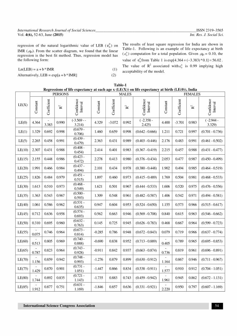
The results of least square regression for India are shown in
Table-1. Following is an example of life expectancy at birth
( 0
0e ) computation for a total population. Given 1q0 = 0.10, the
value of 0
0e from Table 1 is 4.364 ( 3.383)*0.1exp[ ] 56.02+ − = .
The value of R2
associated with 0
0e is 0.99 implying high
acceptability of the model.
Table-1
Regressions of life expectancy at each age x (LE(X)) on life expectancy at birth (LE(0)), India
LE(X)
PERSONS MALES FEMALES
Const
ant
Coef
fici
ent
R2
Conf
iden
ce
Inte
rval
Const
ant
Coef
fici
ent
R2
Conf
iden
ce
Inte
rval
Const
ant
Coef
fici
ent
R2
Conf
iden
ce
Inte
rval
LE(0) 4.364 -
3.383 0.990
(-3.569 - -
3.214) 4.329 -3.072 0.992
( -2.358 -
2.425) 4.400 -3.701 0.983
( -2.944 -
3.329)
LE(1) 1.329 0.692 0.998 (0.679 -
0.706) 1.460 0.659 0.998 (0.642 - 0.666) 1.211 0.721 0.997 (0.701 - 0.736)
LE(5) 2.265 0.458 0.991 (0.439 -
0.479) 2.363 0.431 0.989 (0.403 - 0.446) 2.176 0.483 0.991 (0.461 - 0.502)
LE(10) 2.307 0.431 0.988 (0.408 -
0.454) 2.414 0.401 0.983 (0.367 - 0.419) 2.215 0.457 0.988 (0.431 - 0.477)
LE(15) 2.155 0.448 0.986 (0.423 -
0.472) 2.278 0.413 0.980 (0.376 - 0.434) 2.053 0.477 0.987 (0.450 - 0.499)
LE(20) 1.991 0.466 0.984 (0.437 -
0.494) 2.101 0.434 0.978 (0.380 - 0.448) 1.902 0.494 0.985 (0.464 - 0.519)
LE(25) 1.826 0.484 0.979 (0.451 -
0.515) 1.897 0.460 0.973 (0.415 - 0.489) 1.769 0.504 0.981 (0.468 - 0.533)
LE(30) 1.613 0.510 0.973 (0.468 -
0.549) 1.621 0.501 0.967 (0.444 - 0.533) 1.606 0.520 0.975 (0.476 - 0.556)
LE(35) 1.363 0.543 0.967 (0.500 -
0.593) 1.309 0.548 0.961 (0.482 - 0.587) 1.406 0.542 0.971 (0.494 - 0.581)
LE(40) 1.061 0.586 0.962 (0.531 -
0.635) 0.947 0.604 0.953 (0.524 - 0.650) 1.155 0.573 0.966 (0.515 - 0.617)
LE(45) 0.712 0.636 0.958 (0.574 -
0.693) 0.562 0.663 0.946 (0.569 - 0.708) 0.840 0.615 0.963 (0.546 - 0.662)
LE(50) 0.310 0.695 0.960 (0.632 -
0.763) 0.145 0.725 0.945 (0.626 - 0.783) 0.468 0.667 0.964 (0.599 - 0.723)
LE(55) -
0.075 0.746 0.964
(0.673 -
0.814) -0.285 0.786 0.948 (0.672 - 0.843) 0.079 0.719 0.966 (0.637 - 0.774)
LE(60) -
0.513 0.805 0.969
(0.740 -
0.888) -0.690 0.838 0.952 (0.713 - 0.889)
-
0.405 0.789 0.965 (0.695 - 0.853)
LE(65) -
0.787 0.823 0.964
(0.743 -
0.928) -0.911 0.842 0.937 (0.663 - 0.874)
-
0.736 0.819 0.961 (0.696 - 0.891)
LE(70) -
1.156 0.859 0.942
(0.748 -
0.993) -1.276 0.879 0.899 (0.630 - 0.912)
-
1.164 0.867 0.946 (0.711 - 0.967)
LE(75) -
1.429 0.870 0.901
(0.731 -
1.051) -1.447 0.866 0.834 (0.538 - 0.911)
-
1.577 0.910 0.912 (0.704 - 1.051)
LE(80) -
1.744 0.892 0.835
(0.721 -
1.143) -1.735 0.883 0.743 (0.459 - 0.942)
-
1.961 0.945 0.862 (0.672 - 1.131)
LE(85) -
1.912 0.877 0.751
(0.631 -
1.169) -1.846 0.857 0.636 (0.331 - 0.921)
-
2.220 0.950 0.797 (0.607 - 1.169)
International Research Journal of Social Sciences____________________________________________________ISSN 2319–3565
Vol. 4(6), 52-63, June (2015) Int. Res. J. Social Sci.
International Science Congress Association 55
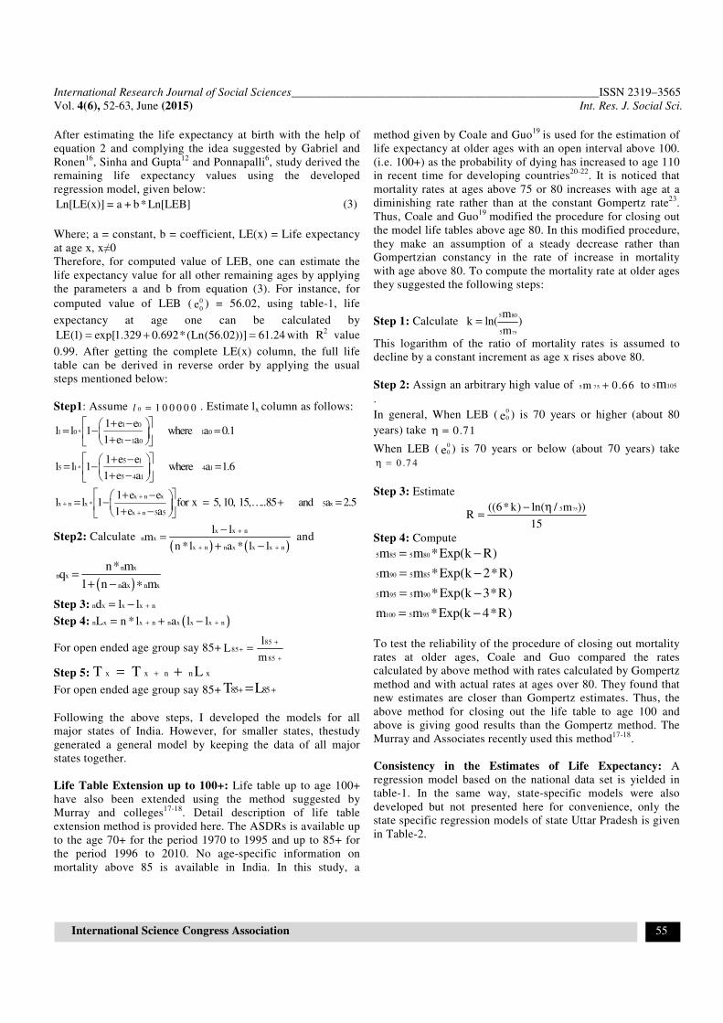
After estimating the life expectancy at birth with the help of
equation 2 and complying the idea suggested by Gabriel and
Ronen16
, Sinha and Gupta12
and Ponnapalli6, study derived the
remaining life expectancy values using the developed
regression model, given below:
Ln[LE(x)] = a + b*Ln[LEB]
(3)
Where; a = constant, b = coefficient, LE(x) = Life expectancy
at age x, x≠0
Therefore, for computed value of LEB, one can estimate the
life expectancy value for all other remaining ages by applying
the parameters a and b from equation (3). For instance, for
computed value of LEB ( 0
0e ) = 56.02, using table-1, life
expectancy at age one can be calculated by
1.329 0.692*(Ln(56.0LE( 2))1) exp[ ] 61.24+= = with R2
value
0.99. After getting the complete LE(x) column, the full life
table can be derived in reverse order by applying the usual
steps mentioned below:
Step1: Assume 0 1 0 0 0 0 0l = . Estimate lx column as follows:
1 01 0 * 1 0
1 1 0
5 15 1* 4 1
5 4 1
x n xx 5 xn x *
x n 5 5
1 e el l 1 where a 0.1
1 e a
1 e el l 1 where a 1.6
1 e a
1 e el for x 5, 10l 1
1 e a, 15, ..85 and a 2.5
++
+
+ − = − =
+ −
+ − = − =
+ −
+ − = −
+ − + =
= …
Step2: Calculate ( ) ( )
x x nn x
x n n x x x n
l lm
n *l a * l l
+
+ +
−=
+ − and
( )
n xn x
n x n x
n* mq
1 n a m=
+ − ∗
Step 3: n x x x nd l l += −
Step 4: ( )n x x n n x x x nL n * l a l l+ += + −
For open ended age group say 85+85
85
85
lL
m
++
+
=
Step 5: x x n n xT T L+= +
For open ended age group say 85+ 85 85T L+ +=
Following the above steps, I developed the models for all
major states of India. However, for smaller states, thestudy
generated a general model by keeping the data of all major
states together.
Life Table Extension up to 100+: Life table up to age 100+
have also been extended using the method suggested by
Murray and colleges17-18
. Detail description of life table
extension method is provided here. The ASDRs is available up
to the age 70+ for the period 1970 to 1995 and up to 85+ for
the period 1996 to 2010. No age-specific information on
mortality above 85 is available in India. In this study, a
method given by Coale and Guo19
is used for the estimation of
life expectancy at older ages with an open interval above 100.
(i.e. 100+) as the probability of dying has increased to age 110
in recent time for developing countries20-22
. It is noticed that
mortality rates at ages above 75 or 80 increases with age at a
diminishing rate rather than at the constant Gompertz rate23
.
Thus, Coale and Guo19
modified the procedure for closing out
the model life tables above age 80. In this modified procedure,
they make an assumption of a steady decrease rather than
Gompertzian constancy in the rate of increase in mortality
with age above 80. To compute the mortality rate at older ages
they suggested the following steps:
Step 1: Calculate 75
5 80
5
mk ln( )
m=
This logarithm of the ratio of mortality rates is assumed to
decline by a constant increment as age x rises above 80.
Step 2: Assign an arbitrary high value of 5 75m 0.66+ to 5 105m.
In general, When LEB (0
0e ) is 70 years or higher (about 80
years) take 0.71η =
When LEB ( 0
0e ) is 70 years or below (about 70 years) take
0 .7 4η =
Step 3: Estimate
755((6*k) ln( / m ))R
15
− η=
Step 4: Compute
5 85 5 80
5 90 5 85
5 95 5 90
100 5 95
m m *Exp(k R)
m m *Exp(k 2*R)
m m *Exp(k 3*R)
m m *Exp(k 4*R)
= −
= −
= −
= −
To test the reliability of the procedure of closing out mortality
rates at older ages, Coale and Guo compared the rates
calculated by above method with rates calculated by Gompertz
method and with actual rates at ages over 80. They found that
new estimates are closer than Gompertz estimates. Thus, the
above method for closing out the life table to age 100 and
above is giving good results than the Gompertz method. The
Murray and Associates recently used this method17-18
.
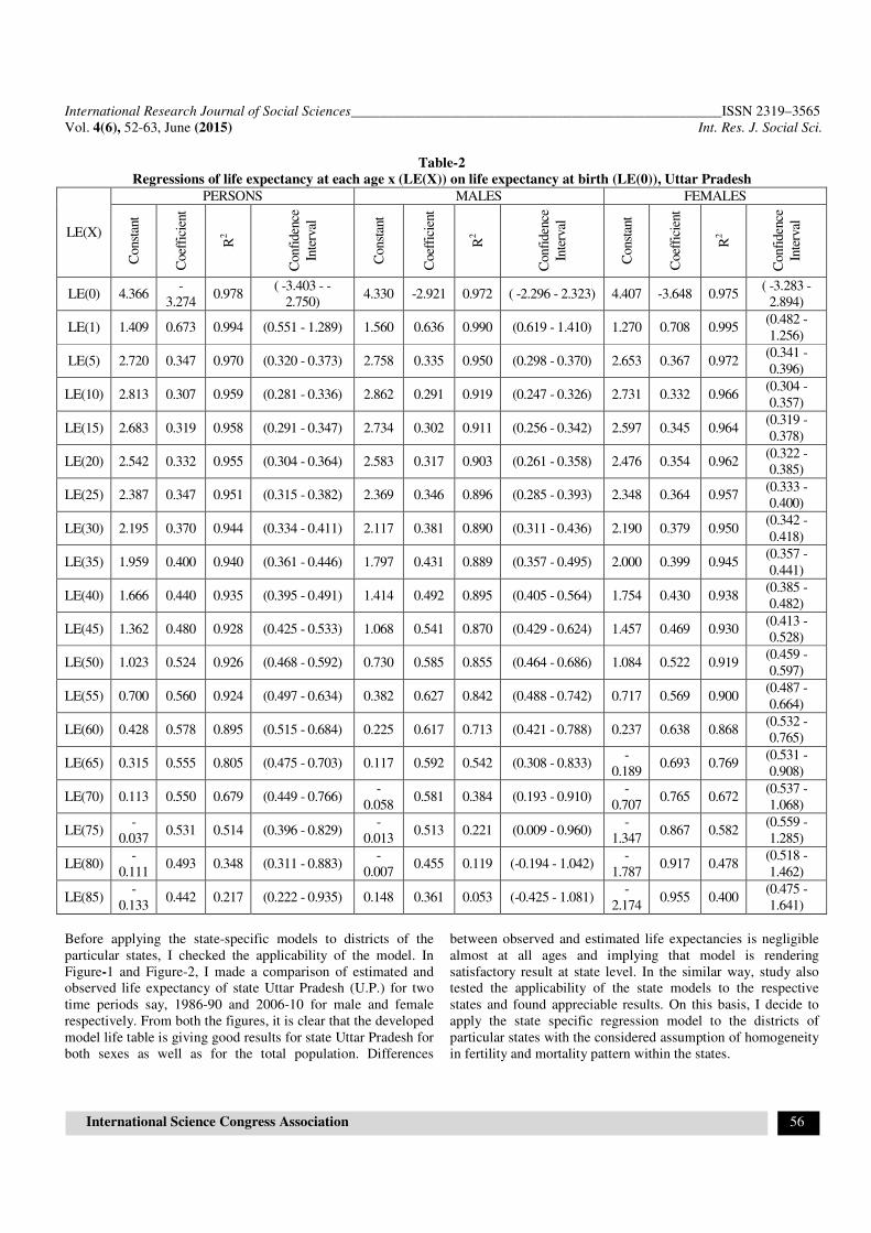
Consistency in the Estimates of Life Expectancy: A
regression model based on the national data set is yielded in
table-1. In the same way, state-specific models were also
developed but not presented here for convenience, only the
state specific regression models of state Uttar Pradesh is given
in Table-2.
International Research Journal of Social Sciences____________________________________________________ISSN 2319–3565
Vol. 4(6), 52-63, June (2015) Int. Res. J. Social Sci.
International Science Congress Association 56
Table-2
Regressions of life expectancy at each age x (LE(X)) on life expectancy at birth (LE(0)), Uttar Pradesh
LE(X)
PERSONS MALES FEMALES
Const
ant
Coef
fici
ent
R2
Confi
den
ce
Inte
rval
Const
ant
Coef
fici
ent
R2
Confi
den
ce
Inte
rval
Const
ant
Coef
fici
ent
R2
Confi
den
ce
Inte
rval
LE(0) 4.366 -
3.274 0.978
( -3.403 - -
2.750) 4.330 -2.921 0.972 ( -2.296 - 2.323) 4.407 -3.648 0.975
( -3.283 -
2.894)
LE(1) 1.409 0.673 0.994 (0.551 - 1.289) 1.560 0.636 0.990 (0.619 - 1.410) 1.270 0.708 0.995 (0.482 -
1.256)
LE(5) 2.720 0.347 0.970 (0.320 - 0.373) 2.758 0.335 0.950 (0.298 - 0.370) 2.653 0.367 0.972 (0.341 -
0.396)
LE(10) 2.813 0.307 0.959 (0.281 - 0.336) 2.862 0.291 0.919 (0.247 - 0.326) 2.731 0.332 0.966 (0.304 -
0.357)
LE(15) 2.683 0.319 0.958 (0.291 - 0.347) 2.734 0.302 0.911 (0.256 - 0.342) 2.597 0.345 0.964 (0.319 -
0.378)
LE(20) 2.542 0.332 0.955 (0.304 - 0.364) 2.583 0.317 0.903 (0.261 - 0.358) 2.476 0.354 0.962 (0.322 -
0.385)
LE(25) 2.387 0.347 0.951 (0.315 - 0.382) 2.369 0.346 0.896 (0.285 - 0.393) 2.348 0.364 0.957 (0.333 -
0.400)
LE(30) 2.195 0.370 0.944 (0.334 - 0.411) 2.117 0.381 0.890 (0.311 - 0.436) 2.190 0.379 0.950 (0.342 -
0.418)
LE(35) 1.959 0.400 0.940 (0.361 - 0.446) 1.797 0.431 0.889 (0.357 - 0.495) 2.000 0.399 0.945 (0.357 -
0.441)
LE(40) 1.666 0.440 0.935 (0.395 - 0.491) 1.414 0.492 0.895 (0.405 - 0.564) 1.754 0.430 0.938 (0.385 -
0.482)
LE(45) 1.362 0.480 0.928 (0.425 - 0.533) 1.068 0.541 0.870 (0.429 - 0.624) 1.457 0.469 0.930 (0.413 -
0.528)
LE(50) 1.023 0.524 0.926 (0.468 - 0.592) 0.730 0.585 0.855 (0.464 - 0.686) 1.084 0.522 0.919 (0.459 -
0.597)
LE(55) 0.700 0.560 0.924 (0.497 - 0.634) 0.382 0.627 0.842 (0.488 - 0.742) 0.717 0.569 0.900 (0.487 -
0.664)
LE(60) 0.428 0.578 0.895 (0.515 - 0.684) 0.225 0.617 0.713 (0.421 - 0.788) 0.237 0.638 0.868 (0.532 -
0.765)
LE(65) 0.315 0.555 0.805 (0.475 - 0.703) 0.117 0.592 0.542 (0.308 - 0.833) -
0.189 0.693 0.769
(0.531 -
0.908)
LE(70) 0.113 0.550 0.679 (0.449 - 0.766) -
0.058 0.581 0.384 (0.193 - 0.910)
-
0.707 0.765 0.672
(0.537 -
1.068)
LE(75) -
0.037 0.531 0.514 (0.396 - 0.829)
-
0.013 0.513 0.221 (0.009 - 0.960)
-
1.347 0.867 0.582
(0.559 -
1.285)
LE(80) -
0.111 0.493 0.348 (0.311 - 0.883)
-
0.007 0.455 0.119 (-0.194 - 1.042)
-
1.787 0.917 0.478
(0.518 -
1.462)
LE(85) -
0.133 0.442 0.217 (0.222 - 0.935) 0.148 0.361 0.053 (-0.425 - 1.081)
-
2.174 0.955 0.400
(0.475 -
1.641)
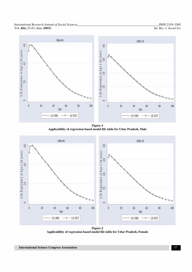
Before applying the state-specific models to districts of the
particular states, I checked the applicability of the model. In
Figure-1 and Figure-2, I made a comparison of estimated and
observed life expectancy of state Uttar Pradesh (U.P.) for two
time periods say, 1986-90 and 2006-10 for male and female
respectively. From both the figures, it is clear that the developed
model life table is giving good results for state Uttar Pradesh for
both sexes as well as for the total population. Differences
between observed and estimated life expectancies is negligible
almost at all ages and implying that model is rendering
satisfactory result at state level. In the similar way, study also
tested the applicability of the state models to the respective
states and found appreciable results. On this basis, I decide to
apply the state specific regression model to the districts of
particular states with the considered assumption of homogeneity
in fertility and mortality pattern within the states.
International Research Journal of Social Sciences____________________________________________________ISSN 2319–3565
Vol. 4(6), 52-63, June (2015) Int. Res. J. Social Sci.
International Science Congress Association 57
Figure-1
Applicability of regression based model life table for Uttar Pradesh, Male
Figure-2
Applicability of regression based model life table for Uttar Pradesh, Female
02
04
06
0L
ife
Ex
pec
tan
cy a
t A
ge
x (
in y
ears
)
0 20 40 60 80 100Age
LE OBS LE EST
1986-90
02
04
06
08
0L
ife
Ex
pec
tan
cy a
t A
ge
x (
in y
ears
)
0 20 40 60 80 100Age
LE OBS LE EST
2006-10
02
04
06
0L
ife
Ex
pec
tan
cy a
t A
ge
x (
in y
ears
)
0 20 40 60 80 100Age
LE OBS LE EST
1986-90
02
04
06
08
0L
ife
Ex
pec
tan
cy a
t A
ge
x (
in y
ears
)
0 20 40 60 80 100Age
LE OBS LE EST
2006-10

International Research Journal of Social Sciences____________________________________________________ISSN 2319–3565
Vol. 4(6), 52-63, June (2015) Int. Res. J. Social Sci.
International Science Congress Association 58
Results and Discussions
To demonstrate the results in a compact manner, I created
figures for life expectancy estimates at different ages using the
software ARCGIS version 1024
. Since, it is not possible to
explain the differentials at each age mortality values among all
districts, so I choose the life expectancy at age 0, 15 and 60 to
explain differentials as these ages have prominent changes in
life expectancy values.
District level variation in Life Expectancy at Birth by Sex:
Life expectancy at birth (LEB) is one of the most desirable
indicators in demographic and health analysis. It manifests the
average number of years that a newborn is expected to survive
under the current schedule of mortality. Life expectancy at birth is
viewed as a proxy measure for various dimensions of nutrition,
good health, education, etc. Besides, it is used in the construction
of the human development index (HDI). Therefore, LEB is of
importance in formulating the population policies at national and
sub-national level. However, the heterogeneity in health and
development within the country leads the different mortality
conditions and henceforth contribute the variation in life
expectancy value at the district level.
In the present section, the study discussed the district level
variation in life expectancy at birth value for India for total,
male, and female population as well. Figure 3 to 5 show the
distribution of life expectancy at birth among the districts of
India for the census year 2001 for total, male and female
population respectively. Life expectancy at birth for both sex
combined is ranging between 45.9 years to 70.2. However, the
range for males is 46.2 to 69.0 years and for a female it is 44.4
to 71.2 years. Examination for district variation reveals that
life expectancy at birth (LEB) is highest for district Udupi of
state Karnataka followed by Mahe of Pondicherry. The lowest
LEB for both sex combined is noticed in district East Kameng
of Arunachal Pradesh. For the male, highest LEB is observed
in Pune of state Maharashtra and for female in Udupi. One
salient feature in district pattern of mortality is the very low
value of male and female LEB for districts Kargil of Jammu
and Kashmir and East Kameng of Arunachal Pradesh. The
study observed a significant variation in life expectancy values
across gender and district as well. The highest gender
difference in LEB is observed in Sheohar district of state
Bihar. In Sheohar, male have 6.3 years more LEB than female.
Figure-3
Distribution of Life Expectancy at Birth in India, 2001, Total

International Research Journal of Social Sciences____________________________________________________ISSN 2319–3565
Vol. 4(6), 52-63, June (2015) Int. Res. J. Social Sci.
International Science Congress Association 59
Figure-4
Distribution of Life Expectancy at Birth in India, 2001, Male
Figure-5
Distribution of Life Expectancy at Birth in India, 2001, Female
International Research Journal of Social Sciences____________________________________________________ISSN 2319–3565
Vol. 4(6), 52-63, June (2015) Int. Res. J. Social Sci.
International Science Congress Association 60
According to Census 2001, the overall literacy rate in district Udupi
was 81.3 percent that is much greater than the national average
(64.8 percent)25
. The health facility and accessibility are found good
in Udupi. Moreover, Udupi is considered in the better performing
district of state Karnataka in terms of safe delivery, live births, a
high level of full vaccination coverage, receiving the BCG
vaccination. In addition, 99 percent women got the minimum three
Antenatal Care (ANC)26
. All these factors lead the lowinfant deaths
and hence resulting in high level of LEB in district Udupi. In the
same way, Mahe is one of the important districts of Union Territory
Pondicherry. It is primarily urban and having overall literacy rate
above 95 percent. The prevalence of women having minimum three
ANC is about 99 percent. The high coverage of BCG and other
vaccination are leaving the better health outcome26
. East Kameng is
primarily rural area. Only 46 percent of currently married women
received any ANC and 20 percent institutional deliveries were
observed. Only 7 percent of women were aware of danger signs of
pneumonia26
. Thus, insufficient utilization of health services are
affecting the child health and hence turning out with a lower life
expectancy at birth.
District level variation in Life Expectancy at age 15 by Sex: In
the last two decades, most of the developing countries are
experiencing an increase in longevity and decline in infant and
child mortality. However, this could not be extending to an infinite
length of life. It is associated with the less premature mortality,
higher life expectancy and healthy and disease free life. Presently
India is experiencing the double burden of disease. While the
reduction of infant and child mortality due to infectious disease is
still incomplete, the increment in non-communicable disease is
observed among adults. Thus, the prevention of deaths among
children and adults is significant public health goal at this moment.
However, there exist a very considerable diversity both within and
among countries/states/districts about mortality experience of
adults. This diversity has been well captured and described in
numerous studies at national, as well as state level but did not
explain at the district level. So, the present section deals with
explaining the variation in young adult mortality by considering the
life expectancy at age 15 as an indicator of young adult mortality.
Figure 6 to 8 show the distribution of life expectancy at age 15 by
districts of India for the census year 2001 for total, male and female
population respectively. For a total population, life expectancy at
age 15 (LE(15)) lies between 43.5 to 58.9 years. The lowest LE(15)
is observed for Kargil (43.5 years) of state Jammu and Kashmir and
highest is noticed for Rupnagar (58.9 years) of state Punjab. For the
male, minimum life expectancy at age 15 is found in Kargil and
highest for Hanumangarh (56.9 years) of Rajasthan. Unlike the
male, for female lowest LE(15) is remarked for Kargil (41.6 years).
The highest LE(15) for female (61.0 years) is detected in district
Rupnagar. The variation in life expectancy at adult ages can be
explained through lifestyle factors (like overeating, obesity,
physical activity, etc.), health behavior (like smoking, alcohol, diet,
etc.), health condition (self-reported status) and physiological
influences (height, weight, stress, Genetic, etc.). It is observed that
the other leading cause of variation in adult mortality is certain
infectious and parasitic diseases like tuberculosis, disease of the
respiratory system27
.
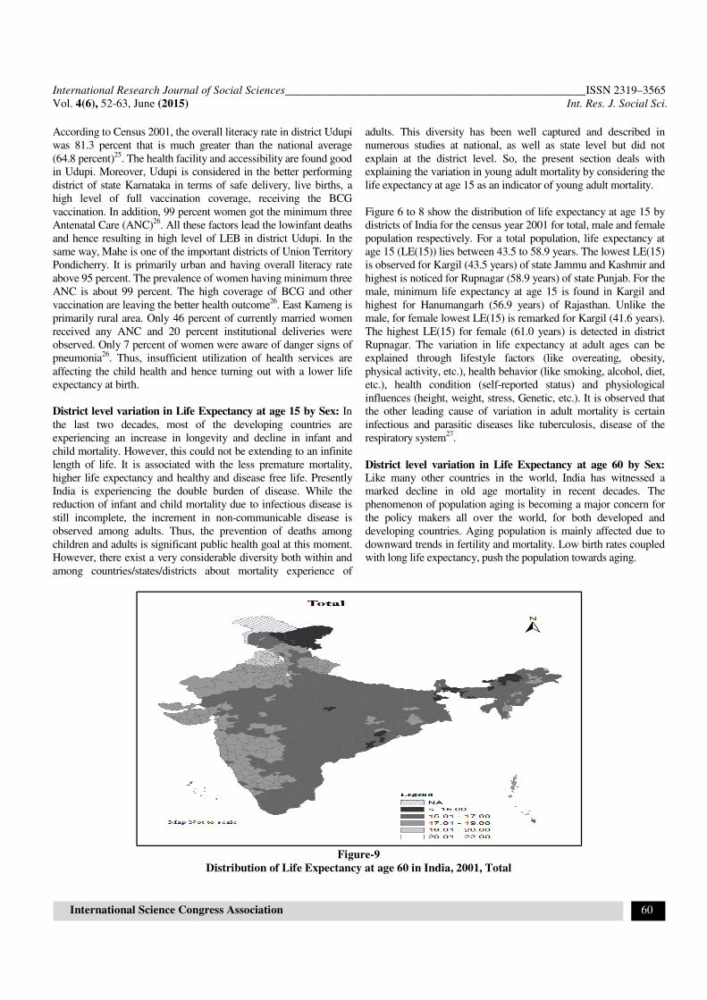
District level variation in Life Expectancy at age 60 by Sex:
Like many other countries in the world, India has witnessed a
marked decline in old age mortality in recent decades. The
phenomenon of population aging is becoming a major concern for
the policy makers all over the world, for both developed and
developing countries. Aging population is mainly affected due to
downward trends in fertility and mortality. Low birth rates coupled
with long life expectancy, push the population towards aging.
Figure-9
Distribution of Life Expectancy at age 60 in India, 2001, Total

International Research Journal of Social Sciences____________________________________________________ISSN 2319–3565
Vol. 4(6), 52-63, June (2015) Int. Res. J. Social Sci.
International Science Congress Association 61
Figure-10
Distribution of Life Expectancy at age 60 in India, 2001, Male
Figure-11
Distribution of Life Expectancy at age 60 in India, 2001, Female
International Research Journal of Social Sciences____________________________________________________ISSN 2319–3565
Vol. 4(6), 52-63, June (2015) Int. Res. J. Social Sci.
International Science Congress Association 62
Figure 9 to 10 deliver the distribution of life expectancy at 60
(LE(60)) for districts of India for total, male and female
population respectively. Among males and female, lowest
LE(60) is detected for district Kargil (11.2 years and 11.8 years
respectively) of state Jammu and Kashmir; whereas highest is
observed for Rupnagar (18.8 years and 21.1 years respectively)
of Punjab. The highest gender difference in LE(60) value is
noticed in districts Bhatinda (2.5 years) and Mansa (2.5 years)
of state Punjab.
Conclusion
The primary objective of the United Nations study had been “to
render a technique with the support of which the mortality level
and its probable age variation can be estimated approximately”
using basic information on infant mortality rates. However, the
indefiniteness of this technique has made it hard to determine
what the most suitable statistical method of obtaining this
procedure might be16
. Thus, more specifically, the aim of this
paper is to supply the best linear regression estimates; best in
the sense of high value of the coefficient of determination (R2)
by using the least square procedure.The study has suggested that
there is only a slight variation between the computed and
observed estimates. Hence, the use of regression technique also
gives very satisfactory estimates of life expectancy value. To
furnish the separate results for each sex, different regression
equation are derived and yielded in the results.
The present study also made an attempt to develop a mortality
database at small area level like district using the information
only on infant mortality rate by applying state-level regression
equations. The database comprises of information on life
expectancy and hence other mortality indicators like number of
survivors; total person-years lived, etc. can be derived with the
help of life expectancy estimate. This mortality database can be
considered as the latest information at the district level. The
analysis is done for all districts of major states of India for
Census year 2001.
Examination for district variation reveals that life expectancy at
birth (LEB) is highest (70.2 years) for district Udupi of state
Karnataka followed by Pune (69.7 years) of Maharashtra.
However, for male highest (69.0 years) LEB is observed in Pune
and Sangli of Maharashtra and for female (71.2 years) in Udupi
of Karnataka. The study found significant variation in life
expectancy values across gender and district as well. An
important finding is that the district has high LEB, also have a
high level of life expectancy at age 15 and 60 and vice versa.
Finding shows that different age group mortality is correlated.
At the same time, it has also brought out the extent of mortality
variation across districts within and between states in the
country. Thus, results clearly affirm that the united approach of
health interventions and policies will not work properly and
henceforth will not help in reducing mortality at the smaller area
level. So, the study recommends for different health
interventions at district and lower level. From a policy point of
view, information linked to mortality rates are needed
continuously not only for prioritizing action but also for
tracking progress in these indicators. Despite the
implementation of decentralization in India, it is very difficult to
get a direct estimate at the district level. One has to rely on the
decennial information from the census by employing an indirect
approach to estimating the district indicators. Indirect estimation
always involves some assumptions; thus, there is a need to
improve and regularize the administrative data system
particularly at the smaller area level.
Though, the study has addressed a number of technical issues
related to mortality estimation at the smaller area, the study,
however, has some limitations related to data and measures that
need to be mentioned. First, the study used the age-specific
death rates provided by SRS. Bhatt28
has doubted the
completeness of India’s SRS data. Nevertheless in a study,
Mahapatra29
re-examined the quality of SRS and remarked that
completeness of the data during 1980s but worsen during 1990s
and after that. Therefore, the study assumes that SRS is the
reliable and trusted the source of mortality data in India. The
study focused on the short period (1971-2010), as the mortality
data is available only for this period. The life expectancy
estimation could be done with more significantly unlike the
developed countries, where mortality data is quite reliable and
accurate and available for longer period. In addition, the main
emphasis of the study is the generation of the district level
mortality databasethat required the age-specific death rates as an
input for each district, but it is not available. So, the study
exploited the available information of infant mortality rate only.
Moreover, research work generated the regression model, for
the development of district level model life, which is based on
the data for the period 1971-2010. There is a possibility that the
model would not work appropriately outside this time range. So
it needs to update the model by time. Along with this, the study
assumes that homogeneity in mortality and fertility pattern
within the state which is not possible in practice.
References
1. Bravo J.M. and Malta J., Estimating life expectancy in
small population areas, Presented in Conference of
European Statistics (2010)
2. Murray C.J.L., Ahmad O.B., Lopez A.D. and Salomon J.A.,
WHO System of Model Life Tables. Geneva, World Health
Organization (GPE Discussion Paper No. 8) (2001)
3. Parasuraman S., An Expanded Component Projection
Method with its Application to India, Ph.D. Thesis,
International Institute for Population Sciences, Mumbai,
India (1984)
4. Roy T.K. and Lahiri S., Recent Levels and Trends in
Mortality in India and its major states: An analysis based on
SRS data. In: Srinivasan K et.al., editors, Dynamics of
Population and Famliy Welfare, Himalaya Publishing
House Mumbai(1987)
International Research Journal of Social Sciences____________________________________________________ISSN 2319–3565
Vol. 4(6), 52-63, June (2015) Int. Res. J. Social Sci.
International Science Congress Association 63
5. Malaker C.R. and Roy G.S., Reconstruction of Indian Life
Tables for 1901-1981 and Projection for 1981-2001,
Sankhya: The Indian Journal of Statistics, 52(B), 271-286
(1990)
6. Ponnapalli K.M. and Kambampati P.K., Age Structure of
Mortality in India and its bigger states: A data base for
cross-sectional and time series research, New Delhi: Serials
Publications (2010)
7. RGI (Registrar General of India), SRS Bulletin Sample
Registration System 2010 Vol. 46(1), Office of Registrar
General of India, Ministry of Home Affairs, GOI, New
Delhi (2011)
8. RGI (Registrar General of India) District level estimates of
child mortality in India based on the 2001 census data,
Office of Registrar General of India, Ministry of Home
Affairs, GOI, New Delhi (2009)
9. RGI (Registrar General of India), Sample Registration
System: 1970-2010, Office of Registrar General of India,
Ministry of Home Affairs, GOI, New Delhi (1971-2010)
10. Wang H., Lopez A.D. and Murray C.J.L., Estimating age
specific mortality: a new model life table system with
flexible standard mortality schedules, Paper presented at
XXVII IUSSP International Population Conference, Busan
Korea, 26-31 August, (2013)
11. United Nations, Age and Sex Patterns of Mortality: Model
Life Tables for Under Developed Countries, Population
Studies22, New York, NY: United Nations (1955)
12. Sinha U.P. and Gupta R.B., Model life tables for India.
Mumbai: IIPS (1979)
13. Ponnapalli K.M., Construction of Model Life tables for
India: using SRS based abridged life tables. Poster
presented at Population Association of America (PAA),
Dallas, Texas, 2010 (2010a)
14. Ponnapalli K.M., A Re-Representation of UN Model Life
tables in their simplest format, (2010b)
15. Wilmoth J.R., Canudas R.V., Zureick S. and Sawyer
C.C.A., flexible two-dimensional mortality model for use in
indirect estimation, Annual Meeting of the population
Association of America (PAA), Detroit. MI., Population
Association of America (2009)
16. Gabriel K.R. and Ronen I., Estimates of mortality from
infant mortality rates, Population Studies, 12(2), 164-169
(1958)
17. Murray C.J.L., Ahmad O.B., Lopez A.D. and Salomon
J.A.WHO System of Model Life tables, GPE discussion
Paper series no. 8. WHO Geneva, (2003)
18. Murray C.J.L., Ferguson B.D., Lopez A.D., Guillot M. and
Salomon J.A. et. al., Modified logit life table system:
principles, empirical validation, and application,
Population Studies, 57(2), 165-182 (2003)
19. Coale A.J. and Guo G., Revised regional model life tables
at very low levels of Mortality. Population Index, 55(4),
613-643 (1989)
20. Vaupel J.W., Carey J.R., Christensen K., Johnson T.E. and
Yashin A.I. et.al., Biodemographic Trajectories of
Longevity. Science, 280(5365), 855-860 (1998)
21. Candus R.V., The Model age at Death and shifting
Mortality Hypothesis, Demographic Research, 19(30),
1179-1204, (2008)
22. Kannisto V., Measuring the Compression of Mortality,
Demographic Research, 3(6) (2000)
23. Perks W., On some experiments in the graduation of
mortality statistics, Journal of the Institute of Actuaries, 63,
12-57 (1932)
24. ESRI, ArcGIS Desktop: Release 10. Redlands, CA:
Environmental Systems Research Institute, (2011)
25. ORGI (Office of Registrar General of India), “Census of
India, 2011”, Ministry of Home Affairs Government of
India, New Delhi, India. Weblink http://www.
census2011.co.in/census/district/268-udupi.html (Accessed
on June 26, 2014), (2011a)
26. IIPS (International Institute for Population Sciences),
District Level Household and Facility Survey (DLHS-2),
2004-05, Udupi Report (2006)
27. ORGI (Office of Registrar General of India), Medical
Certification of Cause of Death 2001. Ministry of Home
Affairs, New Delhi, India, (2007)
28. Bhatt P.N.M., Completeness of India’s Sample Registration
System: An Assessment using the General Growth Balance
Method, Population Studies, 56(2),119-134(2001)
29. Mahapatra P., An overview of Sample Registration System
in India. Paper presented at Prince Mahidol Award
conference and Global Health Information forum, at
Bangkok, Thailand, 27-30 January 2010. Retrieved from
http://unstats.un.org/unsd/vitalstatkb/Attachment476.aspx
(Accessed on March 10, 2014), (2010)