Direct Simulation of Interfacial Waves in a High Viscosity Ratio
and Axisymmetric Core Annular Flow
By Runyuan Bai1, Kanchan Kelkar2 and Daniel D. Joseph1
1 Department of Aerospace Engineering and Mechanics, University of Minnesota,Minneapolis, MN 55455, USA
2 Innovative Research, Inc., 2800 University Ave. SE., Minneapolis, MN 55414, USA
Abstract
A direct numerical simulation of spatially periodic wavy core flows is carried out
under the assumption that the densities of the two fluids are identical and that the viscosity
of the oil core is so large that it moves as a rigid solid which may nevertheless be deformed
by pressure forces in the water. The waves which develop are asymmetric with steep
slopes in the high pressure region at the front face of the wave crest and shallower slopes at
low pressure region at lee side of the crest. The simulation gives excellent agreement with
the experiments of Bai et al.[1992] on up flow in vertical core flow where axisymmetric
bamboo waves are observed. We find a threshold Reynolds number; the pressure force of
the water on the core relative to a fixed reference pressure is negative for Reynolds
numbers below the threshold and is positive above. The wave length increases with the
holdup ratio when the Reynolds number is smaller than a second threshold and decreases
for larger Reynolds numbers. We verify that very high pressures are generated at
stagnation points on the wave front. It is suggested that the positive pressure force is
required to levitate the core off the wall when the densities are not matched and to center the
core when they are. A further conjecture is that the principal features which govern wavy
core flows cannot be obtained from any theory in which inertia is neglected.
2
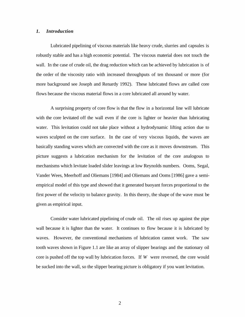
1. Introduction
Lubricated pipelining of viscous materials like heavy crude, slurries and capsules is
robustly stable and has a high economic potential. The viscous material does not touch the
wall. In the case of crude oil, the drag reduction which can be achieved by lubrication is of
the order of the viscosity ratio with increased throughputs of ten thousand or more (for
more background see Joseph and Renardy 1992). These lubricated flows are called core
flows because the viscous material flows in a core lubricated all around by water.
A surprising property of core flow is that the flow in a horizontal line will lubricate
with the core levitated off the wall even if the core is lighter or heavier than lubricating
water. This levitation could not take place without a hydrodynamic lifting action due to
waves sculpted on the core surface. In the case of very viscous liquids, the waves are
basically standing waves which are convected with the core as it moves downstream. This
picture suggests a lubrication mechanism for the levitation of the core analogous to
mechanisms which levitate loaded slider leavings at low Reynolds numbers. Ooms, Segal,
Vander Wees, Meerhoff and Oliemans [1984] and Oliemans and Ooms [1986] gave a semi-
empirical model of this type and showed that it generated buoyant forces proportional to the
first power of the velocity to balance gravity. In this theory, the shape of the wave must be
given as empirical input.
Consider water lubricated pipelining of crude oil. The oil rises up against the pipe
wall because it is lighter than the water. It continues to flow because it is lubricated by
waves. However, the conventional mechanisms of lubrication cannot work. The saw
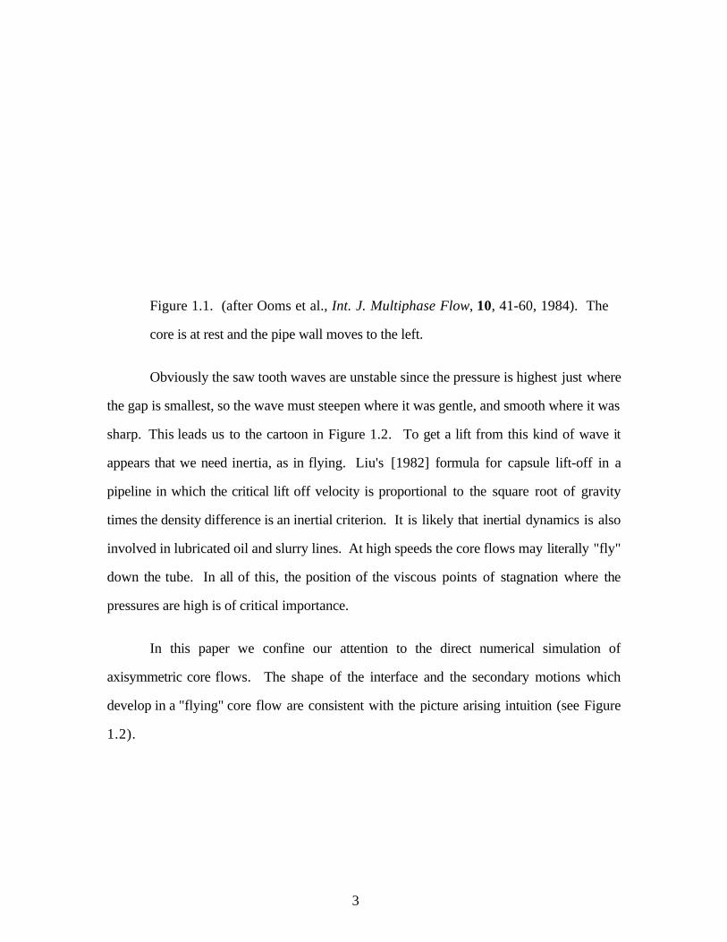
tooth waves shown in Figure 1.1 are like an array of slipper bearings and the stationary oil
core is pushed off the top wall by lubrication forces. If W were reversed, the core would
be sucked into the wall, so the slipper bearing picture is obligatory if you want levitation.
3
Figure 1.1. (after Ooms et al., Int. J. Multiphase Flow, 10, 41-60, 1984). The
core is at rest and the pipe wall moves to the left.
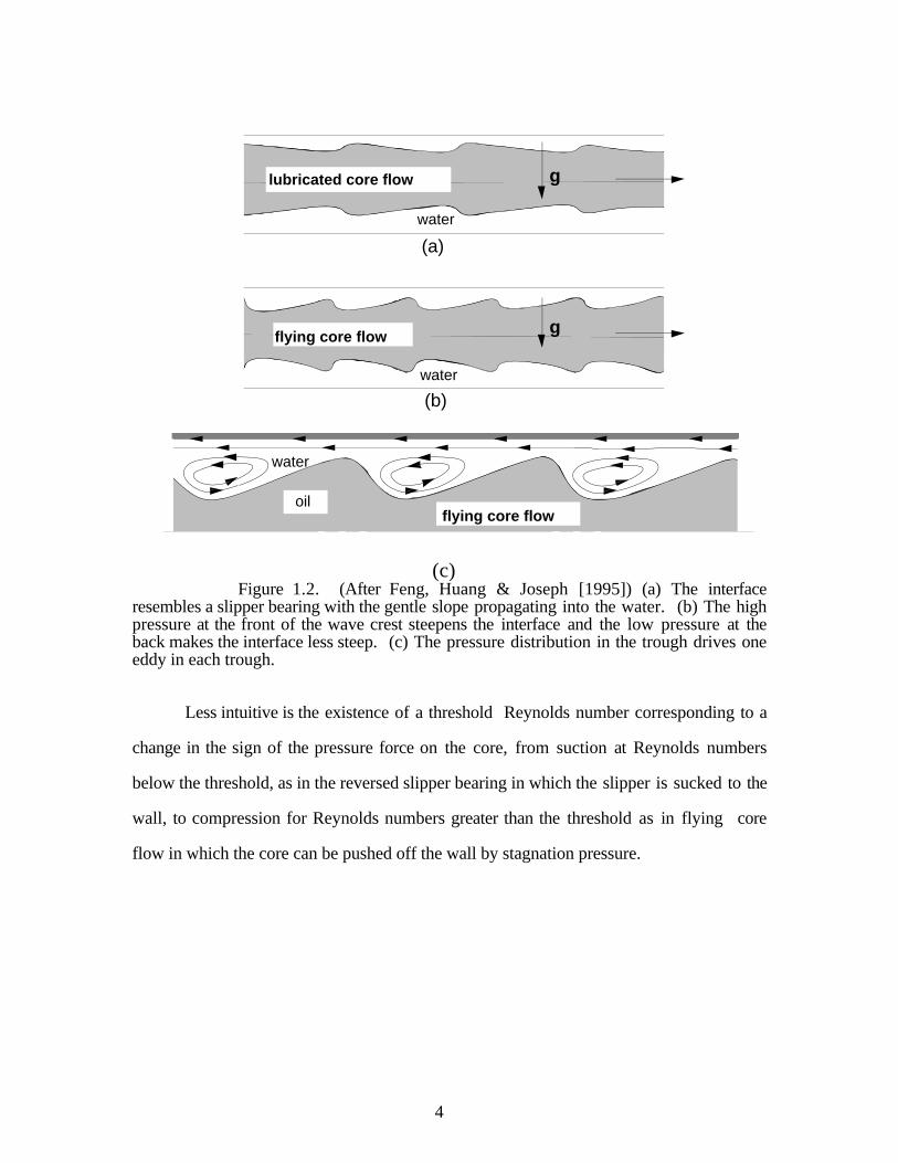
Obviously the saw tooth waves are unstable since the pressure is highest just where
the gap is smallest, so the wave must steepen where it was gentle, and smooth where it was
sharp. This leads us to the cartoon in Figure 1.2. To get a lift from this kind of wave it
appears that we need inertia, as in flying. Liu's [1982] formula for capsule lift-off in a
pipeline in which the critical lift off velocity is proportional to the square root of gravity
times the density difference is an inertial criterion. It is likely that inertial dynamics is also
involved in lubricated oil and slurry lines. At high speeds the core flows may literally "fly"
down the tube. In all of this, the position of the viscous points of stagnation where the
pressures are high is of critical importance.
In this paper we confine our attention to the direct numerical simulation of
axisymmetric core flows. The shape of the interface and the secondary motions which
develop in a "flying" core flow are consistent with the picture arising intuition (see Figure
1.2).
4
(a)
(b)
water
water
lubricated core flow g
gflying core flow
oil
water
flying core flow
(c)Figure 1.2. (After Feng, Huang & Joseph [1995]) (a) The interface
resembles a slipper bearing with the gentle slope propagating into the water. (b) The highpressure at the front of the wave crest steepens the interface and the low pressure at theback makes the interface less steep. (c) The pressure distribution in the trough drives oneeddy in each trough.
Less intuitive is the existence of a threshold Reynolds number corresponding to a
change in the sign of the pressure force on the core, from suction at Reynolds numbers
below the threshold, as in the reversed slipper bearing in which the slipper is sucked to the
wall, to compression for Reynolds numbers greater than the threshold as in flying core
flow in which the core can be pushed off the wall by stagnation pressure.
5
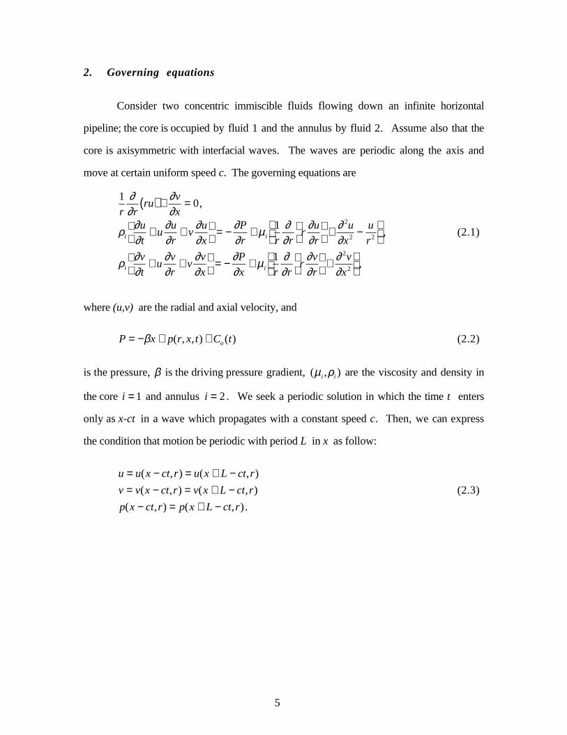
2. Governing equations
Consider two concentric immiscible fluids flowing down an infinite horizontal
pipeline; the core is occupied by fluid 1 and the annulus by fluid 2. Assume also that the
core is axisymmetric with interfacial waves. The waves are periodic along the axis and
move at certain uniform speed c. The governing equations are
1r
∂∂r
ru( ) + ∂v
∂x= 0,
ρi
∂u
∂t+ u
∂u
∂r+ v
∂u
∂x
= − ∂P
∂r+ µ i
1r
∂∂r
r∂u
∂r
+ ∂ 2u
∂x2 − u
r2
, (2.1)
ρi
∂v
∂t+ u
∂v
∂r+ v
∂v
∂x
= − ∂P
∂x+ µ i
1r
∂∂r
r∂v
∂r
+ ∂ 2v
∂x2
,
where (u,v) are the radial and axial velocity, and
P = −βx + p(r, x,t) + Co(t) (2.2)
is the pressure, β is the driving pressure gradient, (µ i ,ρi ) are the viscosity and density in
the core i = 1 and annulus i = 2 . We seek a periodic solution in which the time t enters
only as x-ct in a wave which propagates with a constant speed c. Then, we can express
the condition that motion be periodic with period L in x as follow:
u = u(x − ct,r) = u(x + L − ct,r)
v = v(x − ct,r) = v(x + L − ct,r) (2.3)
p(x − ct,r) = p(x + L − ct,r) .
6
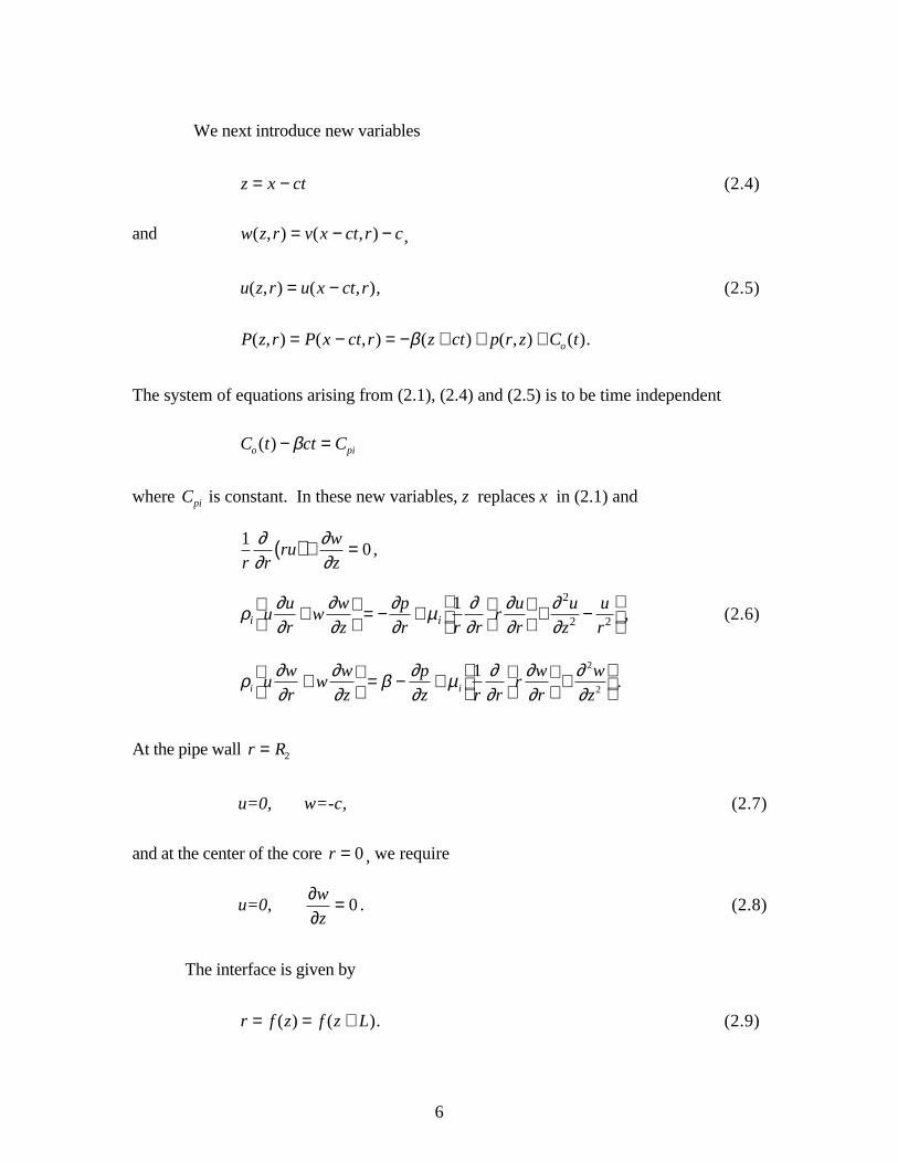
We next introduce new variables
z = x − ct (2.4)
and w(z,r) = v(x − ct,r) − c,
u(z,r) = u(x − ct,r), (2.5)
P(z,r) = P(x − ct,r) = −β(z + ct) + p(r, z) + Co(t).
The system of equations arising from (2.1), (2.4) and (2.5) is to be time independent
Co(t) − βct = Cpi
where Cpi is constant. In these new variables, z replaces x in (2.1) and
1r
∂∂r
ru( ) + ∂w
∂z= 0 ,
ρi u∂u
∂r+ w
∂w
∂z
= − ∂p
∂r+ µ i
1r
∂∂r
r∂u
∂r
+ ∂ 2u
∂z2 − u
r2
, (2.6)
ρi u∂w
∂r+ w
∂w
∂z
= β − ∂p
∂z+ µ i
1r
∂∂r
r∂w
∂r
+ ∂ 2w
∂z2
.
At the pipe wall r = R2
u=0, w=-c, (2.7)
and at the center of the core r = 0 , we require
u=0, ∂w
∂z= 0 . (2.8)
The interface is given by
r = f (z) = f (z + L). (2.9)
7
Here, between the water and oil, the kinematics condition is
u = dfdt
= ∂f∂t
+ v ∂f∂x
= w ∂f∂z
, (2.10)
and the velocity condition is [[U]] = 0 , where [[•]] = (•)1 − (•)2 and
U = (u,w). (2.11)
The normal stress condition is
−[[P]] + 2Hσ( ) + n •[[2µD U[ ]]]• n = 0 , (2.12)
and the shear stress condition is
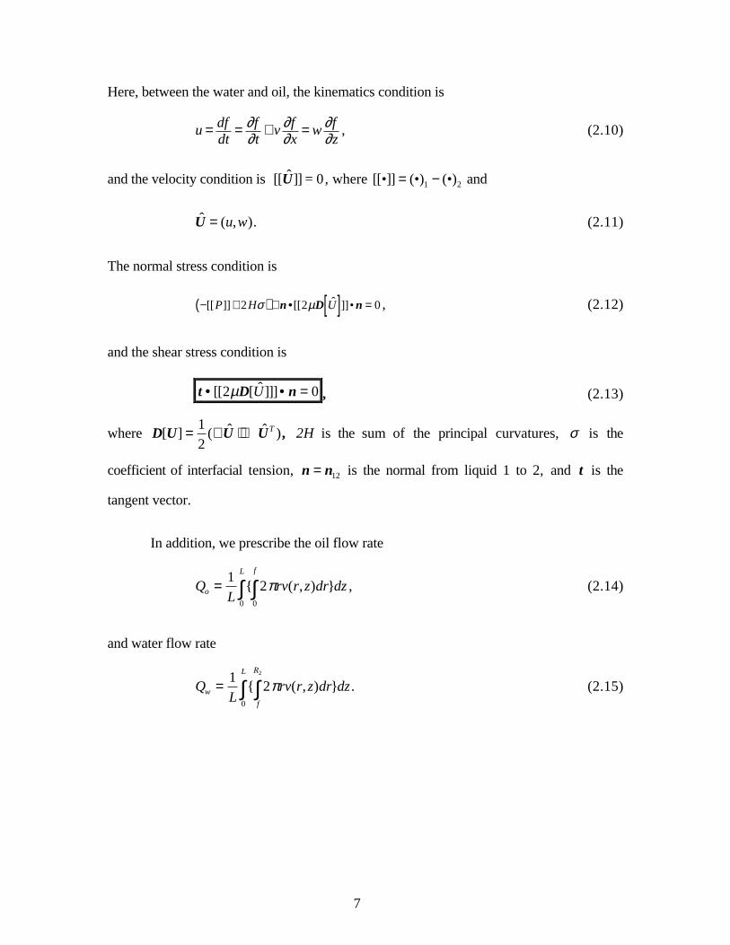
t • [[2µD[U]]]• n = 0 , (2.13)
where D[U] = 12
(∇U + ∇UT ), 2H is the sum of the principal curvatures, σ is the
coefficient of interfacial tension, n = n12 is the normal from liquid 1 to 2, and t is the
tangent vector.
In addition, we prescribe the oil flow rate
Qo = 1L
{ 2πrv(r, z)dr}dz0
f
∫0
L
∫ , (2.14)
and water flow rate
Qw = 1L
{0
L
∫ 2πrv(r, z)dr}dzf
R2
∫ . (2.15)
8
3. Rigid Deformable Core flow
In many situations, the viscosity of the oil is much greater than the viscosity of
water. We shall assume that the core is solid with standing waves on the interface. A
consequence of this assumption is that non-rigid motions of the core may be neglected. In
this rigid deformable core model, the core is stationary (U1 = 0 ) and water moves. The
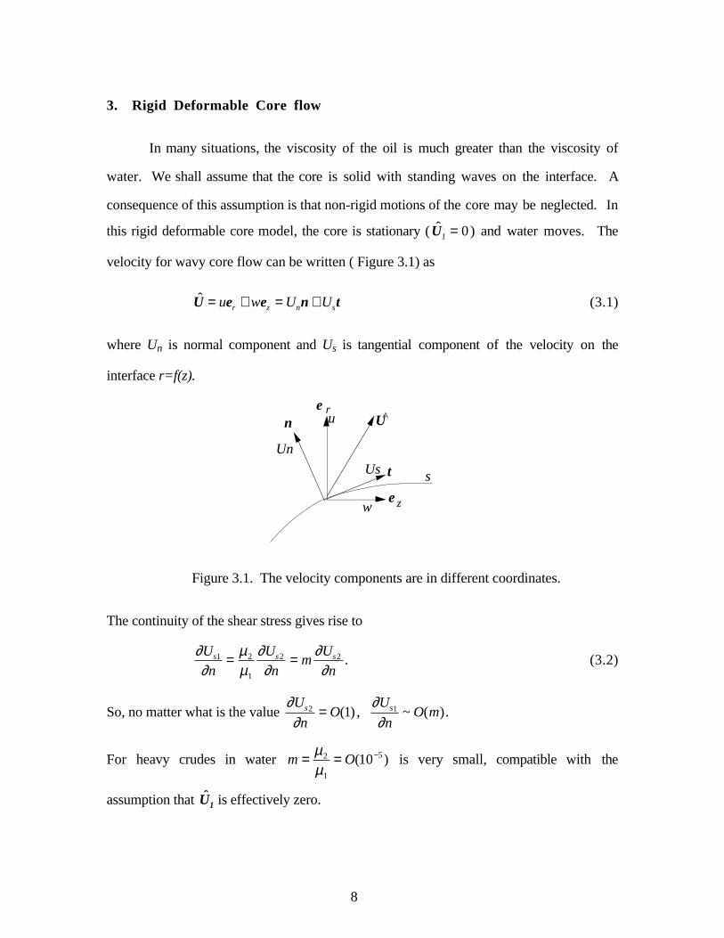
velocity for wavy core flow can be written ( Figure 3.1) as
U = uer + wez = Unn + Ust (3.1)
where Un is normal component and Us is tangential component of the velocity on the
interface r=f(z).
Uu
w
Us
Un
s
ne
e
r
z
^
t
Figure 3.1. The velocity components are in different coordinates.
The continuity of the shear stress gives rise to
∂Us1
∂n= µ2
µ1
∂Us2
∂n= m
∂Us2
∂n. (3.2)
So, no matter what is the value ∂Us2
∂n= O(1) ,
∂Us1
∂n~ O(m).
For heavy crudes in water m = µ2
µ1
= O(10−5 ) is very small, compatible with the
assumption that U1 is effectively zero.
9
From continuity of velocity on the interface, [[U]] = 0, we also obtain that the water
velocity is zero on the interface. Since the relative velocity in the solid core vanishes, the
speed c of the advected wave, in coordinates in which the wall is stationary, is exactly the
core velocity c=w(r,z) which is constant, independent of r and z when r ≤ f (z). In this
case (2.14) reduces to
Qo = πR12c , (3.3)
and R12 = 1
Lf 2 (z)dz
0
L
∫ . (3.4)
The viscous part of the normal stress on the interface vanishes:
n • [[2µD[U]]] • n = 2µ1
∂Un1
∂n− 2µ2
∂Un2
∂n= 0 (3.5)
since∂Us
∂s+ ∂Un
∂n= 0
and on the interface
∂US
∂s= 0 . (3.6)
Therefore, the normal stress balance (2.12) reduces to
[[P]] = 2Hσ . (3.7)
Although the core is assumed to be a deformable rigid body, there is a mass flow of
oil in the pipeline, which is driven by pressure βz . The pressure in the core is
P1 = −βz + Cp1 , (3.8)
while the pressure in the annulus is
P2 = −βz + p(r, z) + Cp2 . (3.9)
10
Since the pressure level is indeterminate we may, without loss of generality, put
Cp2 = 0 . (3.10)
In the water, f ≤ r ≤ R2 , we have
1r
∂∂r
ru( ) + ∂w
∂z= 0
ρ2 u∂u
∂r+ w
∂u
∂z
= − ∂p
∂r+ µ2
1r
∂∂r
r∂u
∂r
+ ∂ 2u
∂z2 − u
r2
(3.11)
ρ2 u∂w
∂r+ w
∂w
∂z
= β − ∂p
∂z+ µ2
1r
∂∂r
r∂w
∂r
+ ∂ 2w
∂z2
.
And in the oil core, 0 < r < f
dP1
dz= −β .
The normal stress balance at r = f which is given by (3.8), then becomes
σ
f 1+ dfdz
2−
σ d2 fdz2
1+ dfdz
2
3/2 = [[P]] = P1 − P2 = C − p . (3.12)
To solve our problem we must prescribe β , and compute c, or we may give c and
compute β . Since the momentum change in one wavelength is zero, we may relate c and
β by the force balance shown in Figure 3.2 and expressed as
AβL = Fz = 2π f (nP2 + tτ) • ezds0
SL
∫ = 2π (nP2 + tτ) • ez f 1 + (df dz)2 dz0
L
∫ ,
= 2π (P2sinθ + τcosθ ) f 1 + (df dz)2 dz0
L
∫ (3.14)
where tanθ = df
dz, (3.15)
11
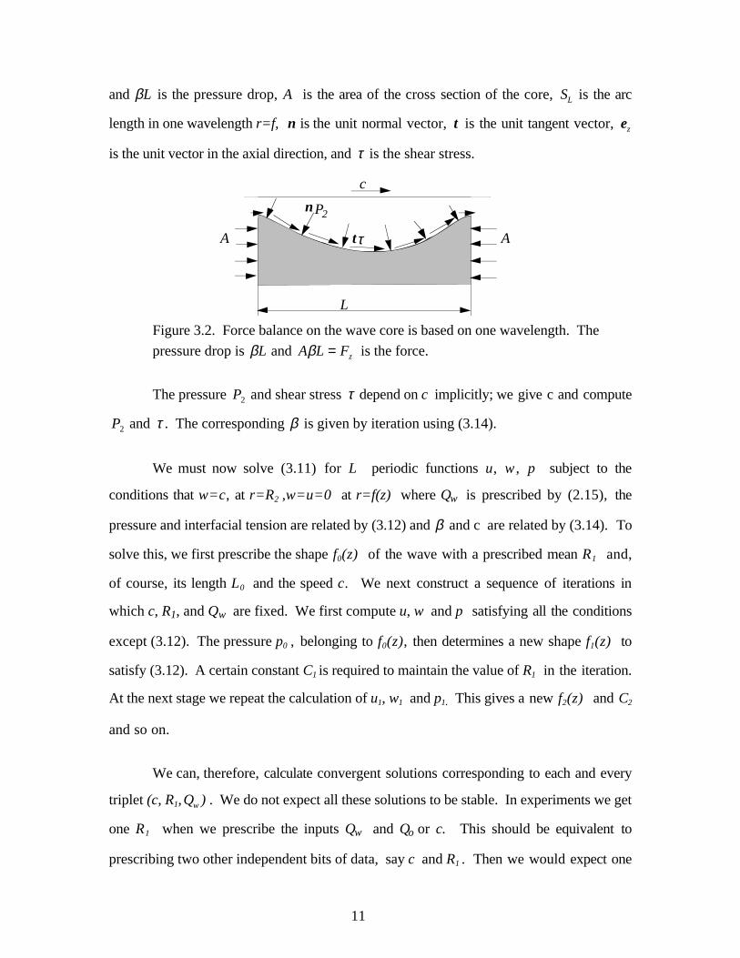
and βL is the pressure drop, A is the area of the cross section of the core, SL is the arc
length in one wavelength r=f, n is the unit normal vector, t is the unit tangent vector, ez
is the unit vector in the axial direction, and τ is the shear stress.
c
L
A A
P2
τ
n
t
Figure 3.2. Force balance on the wave core is based on one wavelength. The
pressure drop is βL and AβL = Fz is the force.
The pressure P2 and shear stress τ depend on c implicitly; we give c and compute
P2 and τ . The corresponding β is given by iteration using (3.14).
We must now solve (3.11) for L periodic functions u, w , p subject to the
conditions that w=c, at r=R2 ,w=u=0 at r=f(z) where Qw is prescribed by (2.15), the
pressure and interfacial tension are related by (3.12) and β and c are related by (3.14). To
solve this, we first prescribe the shape f0(z) of the wave with a prescribed mean R1 and,
of course, its length L0 and the speed c. We next construct a sequence of iterations in
which c, R1, and Qw are fixed. We first compute u, w and p satisfying all the conditions
except (3.12). The pressure p0 , belonging to f0(z), then determines a new shape f1(z) to
satisfy (3.12). A certain constant C1 is required to maintain the value of R1 in the iteration.
At the next stage we repeat the calculation of u1, w1 and p1. This gives a new f2(z) and C2
and so on.
We can, therefore, calculate convergent solutions corresponding to each and every
triplet (c, R1,Qw ) . We do not expect all these solutions to be stable. In experiments we get
one R1 when we prescribe the inputs Qw and Qo or c. This should be equivalent to
prescribing two other independent bits of data, say c and R1 . Then we would expect one
12
Qw for each c and R1 to appear in experiments, but we calculate a family of solutions for
the given c and R1 and any Qw . When the parameters are taken for perfect core flow, we
get perfect core flow from our simulation; most of these perfect core flows are actually
unstable. Our simulation then can be regarded as giving rise to a one parameter family of
wavy core flows whose stability is yet to be tested.
13
4. The holdup ratio in wavy core flow
The holdup ratio h is the ratio Qo/Qw of volume flow rates to the ratio Vo/Vw of
volume in the pipe:
h = Qo / Qw
Vo / Vw
= Qo Qw
R12 (R2
2 − R12 )
, (4.1)
The holdup ratio depends on the fluid properties and flow parameters but is most strongly
influenced by flow type. Equation (4.1) can be represented as the ratio of superficial
velocities
h = Qo πR12
Qw π(R22 − R1
2 )= c0
cw
, (4.2)
where co = Qo
πR12 , (4.3)
cw = Qw
π(R22 − R1
2 ), (4.4)
and c=co for rigid core flow.
Here, we consider the holdup ratio in perfect core flow and wavy core flow. A
perfect core annular flow has a perfectly cylindrical interface of uniform radius without
waves and is perfectly centered on the pipe axis with an annulus of lubricating water all
around. The velocity W and flow rate Q of a perfect core flow is
Wo (r) = β4µ1
R12 − r2( ) + β
4µ2R2
2 − R12( ) , (4.5)
Ww (r) = β4µ2
R22 − r2( ) , (4.6)
Qo = 2π rWo
0
R1
∫ dr = 2π β16µ1
R14 + β
8µ2(R2
2R12 − R1
4 )
, (4.7)
14
Qw = 2π rWw (r)dr
R1
R2
∫ = 2π β16µ2
R22 − R1
2( )2
. (4.8)
(4.7) and (4.8) can be written as
Qo = − βπR14
8µ2m + 2 a2 −1( )( ), (4.9)
and Qw = − βπR14
8µ2a2 −1( )2
. (4.10)
The ratio of the flow rates, the input ratio, is
γ = Qo
Qw
= m + 2(a2 − 1)(a2 − 1)2 , (4.11)
where m = µ2
µ1
, a = R2
R1
= 1 + 1γ
(1 + 1 + mγ ) .
The oil fraction is given by
η2 = R1
R2
2
= 1a2 = 1
1 + 1γ
1 + 1 + mγ( ), (4.12)
while the water fraction is given by
1 − η2 = 1 − 1
1 + 1γ
1 + 1 + mγ( )=
1 + 1 + mγγ + 1 + 1 + mγ
. (4.13)
The volume ratio is proportional to the fraction ratio. Hence
V0
Vw
= η2
1 − η2 = γ1 + 1 + mγ
. (4.14)
The equation for the holdup ratio is therefore
15
h = Qo / Qw
Vo / Vw
= γγ
1 + 1 + mγ
= 1 + 1 + mγ . (4.15)
For very viscous oil, m ≈ 0, and h ≈ 2.
Now let us consider the holdup ratio for wavy core flow in the system of
coordinates in which the wall is stationary. Given a periodic function f(x-ct) =f(z) with
wave length L, the average diameter of the oil core is R1, where
1L
f 2 (z)dz0
L
∫ = R12 . (4.16)
The input rate for a rigid core is related to the wave speed by
Qo = πR12c = cπ
Lf 2 z( )dz
0
L
∫ (4.17)
Since both water and oil flow rates are specified, the total flow rate at each cross section is
constant:
Qtotal = Qo + Qw = πf 2 (z)c + 2π rv r, z( )drf (z )
R2
∫ (4.18)
where v(r, z) = 0 r = R2
c r = f (z)
and the flow inputs Qo and Qw are independent of z.
Then, the water input can be written as
Qw = Qtotal − Qo = πc f 2 (z) − R12[ ] + 2π rv(r, z)dr
f (z )
R2
∫ (4.19)
independent of z .
Equation (4.19) gives an interesting z dependent decomposition of the constant
water input Qw. We may write (4.19) as
16
Qw = Φ(z) + Ψ (z), (4.20)
where Φ = πC f 2 (z) − R12[ ] (4.21)
and Ψ (z) = 2π rv(r, z)drf (z )
R2
∫ . (4.22)
Suppose that a wave crest at z=0 just touches the pipe wall, f(z)=R2 . In this case, the
water flow Qw is entirely due to the forward motion of the water trapped in troughs and
Ψ (z) = 0 , Φ(0) = πc[R22 − R1
2 ]
so that Φ(z) can be said to represent the trapped water. On the other hand, for perfect core
flow Φ = 0 for all z.
When Qo and Qw are given, the wave speed c and the average diameter of the oil
core depends on the wave shape f (z) . The holdup ratio for wavy core flow is then given
by
h = Qo Qw
R12 (R2
2 − R12 )
= πcR12
πc f 2 − R12[ ] + 2π rvdr
f
R2
∫
R22 − R1
2
R12 . (4.23)
For perfect core annular flow, the flow rate of trapped water is zero since the core
radius is uniform f 2 = R12 . Using W from (4.8) we get h=2 . Let us focus on the flow
rates at the cross section of the wave crest, where f = f max and assume that f max = R2 .
Then the integral in (4.23) vanishes and the holdup ratio is 1. Therefore, the holdup ratio
for wavy core flow is between 1 and 2.
In the transition from a perfect core flow to a wavy core flow, the wave troughs
will carry extra water even if the average diameter of the oil core is unchanged; this
increases the water flow rate. However, when the water flow rate is fixed, the system can
not increase the water flow rate. Therefore, the average diameter of the core will increase,

17
reducing the water flow rate. In the wavy flow, more oil is in the pipe than in perfect core
flow, and the holdup ratio is less than 2. Of course, the speed of the core must decrease
when there is more oil and oil flow rate is fixed.
The pressure gradient β is related to the difference in area of the core at a crest and
average area, this is measured by
d = πc[ f 2 (0) − R12 ]. (4.24)
The gap between the pipe wall and wave crest is smaller when d is larger, provided that the
volume of oil in the pipe is fixed. Smaller gaps imply high friction and large values of the
pressure gradient.
5. Comparison with experiments
Our simulations are for the case in which the density of oil and water are the same;
when they are not the same and the pipe in horizontal, the oil core will rise or sink. Some
representative wave shapes, which look like those in experiments, are for density matched
flows in Figure 5.1.
a
0 1 2 3 4 5
18
b
0 1 2 3 4 5
c
0 1 2 3 4 5
d
0 1 2 3 4 5
e
0 1 2 3 4 5
f
0 1 2 3 4 5
g
0 1 2 3 4 5
h
0 1 2 3 4 5

19
i
0 1 2 3 4 5
Figure 5.1. Selected wave shapes for water lubricated axisymmetric flow of oil and
water with the same density ρ=1.0g/cm3, µ2=0.01 poise and σ=26dyne/cm for oil and
water. The pipe diameter is R2=1.0cm. Qo and Qw are in cm3/sec. The data for each
frame is given as the triplet (R1, Qo, Qw), a (0.37, 4.30, 2.73), b (0.37, 8.6, 5.47 ), c
(0.37, 17.2, 10.93), d (0.41, 10.56, 3.67), e (0.41, 18.48, 6.43), f (0.41, 26.41, 9.19),
g (0.43, 34.85, 8.76), h (0.43, 43.57, 10.96) and i (0.43, 69.71, 17.53). The core is
stationary and the wall moves to the right.
Bai, Chen and Joseph [1992] did experiments and calculated stability results for
vertical axisymmetric core flow in the case when the buoyant force and pressure force on
the oil are both against gravity (up flow). They observed "bamboo" waves for their oil
ρo=0.905g/cm3 and µo=6.01 poise in water with ρw=0.995g/cm3 and µw=0.01 poise. We
have simulated the same flow, with the same parameters except that our core is infinitely
viscous. The results show that µo=6.01 is not yet asymptotically infinitely viscous, but
nevertheless the agreements are satisfactory.
The equations that we used for our simulation are follow. In the water, we have
1r
∂∂r
ru( ) + ∂w
∂z= 0
,
ρ2 u∂u
∂r+ w
∂u
∂z
= − ∂p
∂r+ µ2
1r
∂∂r
r∂u
∂r
+ ∂ 2u
∂z2 − u
r2
, (5.1)
ρ2 u
∂w
∂r+ w
∂w
∂z
= β + ρcg − ∂p
∂z− ρ2g + µ2
1r
∂∂r
r∂w
∂r
+ ∂ 2w
∂z2
.
20
The pressure in the water is
P2 (r, z) = −βz + p(r, z) − ρcgz + C2 (5.2)
while the pressure in the core is
P1 = −βz − ρcgz + C1 (5.3)
where g is gravity and ρc is the composite density of the mixture
ρc = ρ1η2 + (1 − η2 )ρ2, (5.4)
and η = R1
R2
.
We compared wavelengths, wave speeds and wave shapes from our computation
with experiments and the linear theory of stability in Bai, Chen & Joseph [1992]. In our
comparison, the flow parameters are based on the experimental information, such as flow
rates of oil and water, oil volume ratio and holdup ratio. In Bai, Chen and Joseph [1992],
the holdup ratio is a constant 1.39 and the volume ratio of the oil yields the following
formula:
R12
R22 = 1 − 1
1 + 0.72 Qo Qw( ) . (5.5)

21
The results are given in Table 5.1.
input flowrate computations experiments I II no. Q o Q w L (cm) c (cm/s) L (cm) c (cm/s) L (cm) c (cm/s) L (cm) c (cm/s)
1 25.38 13.17 1.32 55.59 1.21 57.7 0.82 79.84 0.79 52.02
2 18.19 13.17 1.66 46.45 1.31 43.28 0.92 80.21 0.96 42.54
3 11.01 13.17 1.70 37.30 1.41 35.65 1.22 79.76 1.22 33.51
4 7.42 13.17 1.33 32.73 1.22 27.81 1.65 77.00 1.33 29.42
5 7.42 6.46 1.77 20.88 1.374 19.16 1.56 58.91 1.25 17.94
6 11.01 6.46 1.66 25.45 1.79 22.90 1.23 58.12 1.16 22.17
7 14.60 6.46 1.39 3 0.02 1.34 28.22 1.05 54.80 1.02 26.68
8 18.19 6.46 1.15 34.59 1.17 31.06 0.95 50.85 0.87 31.33
9 21.78 6.46 0.96 39.17 0.90 36.25 0.86 49.38 0.79 35.71
Table 5.1. Comparison of computed and measured values of the wave speed c and
wave length L with theory of stability. In column I and II, data from Bai, Chen & Joseph
[1992] were computed by linear theory of stability. In column I, the computations werecarried out for the values of Qo and Qw prescribed in the experiments. In column II, the
calculations were done the prescribed Qo and measured value of R1 corresponding to the
observed holdup ratio h=1.39.
The comparison of computed and measured values of the wave speed and
wavelength of bamboo waves is given in Table 5.1. The computed values are slightly
larger than the measured values, due to the fact that motion in the core is neglected with
better agreement for faster flow.
Computed wave shapes and the observed shapes of bamboo waves are compared in
Figure 5.2-5.3. The pictures were taken in a vertical pipeline with motor oil
(ρo = 0.905gm / cm3,µo = 6.01poise) and water (ρw = 0.995gm / cm3,µw = 0.01poise).
Both water and oil flow against gravity. The water flow rate is fixed at 200 cm3/min
while oil flow rate is 429, 825 and 1216 cm3/min respectively.
22
a b
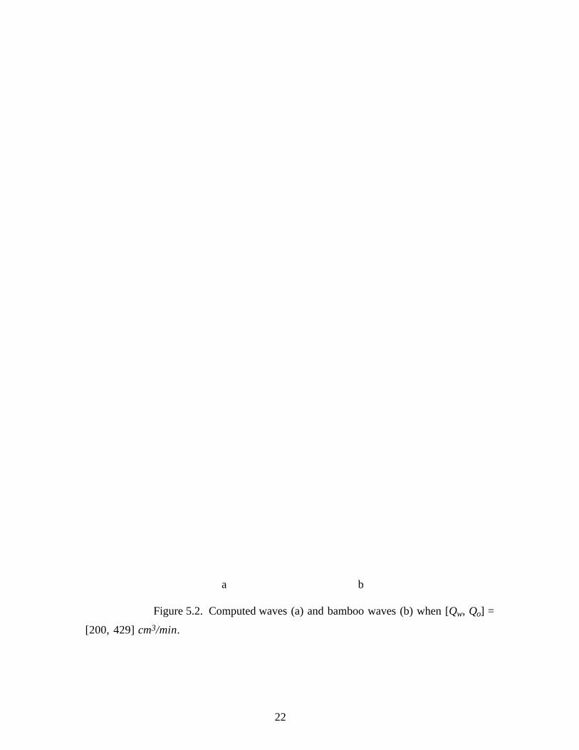
Figure 5.2. Computed waves (a) and bamboo waves (b) when [Qw, Qo] =
[200, 429] cm3/min.
23
a b
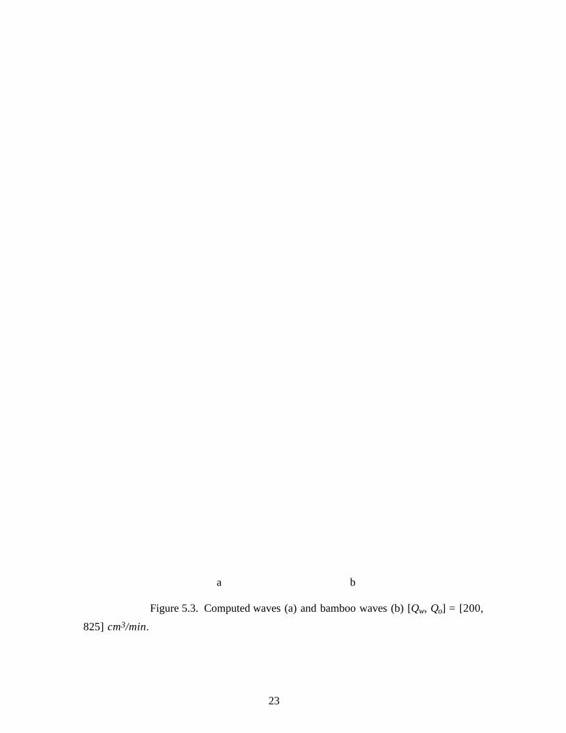
Figure 5.3. Computed waves (a) and bamboo waves (b) [Qw, Qo] = [200,
825] cm3/min.

24
a b
Figure 5.4. Computed waves (a) and bamboo waves (b) [Qw, Qo] = [200,
1216] cm3/min.
25
The computed and observed shapes are alike. In fast flow, the velocity in the oil
core is small compared with the velocity in the annulus and the oil core can be considered to
be a rigid deformable body. In slower flow (Figure 5.2), the flow inside the core is not so
much smaller than the flow in annulus and the stems of the waves are more readily
stretched by buoyancy. Even in this case the agreements are satisfactory.
6. Dimensionless equations
Analysis of this simulation is most useful when carried out in terms of
dimensionless variables. In the dimensional equations, we used following parameters:
(R2, R1, µ2, ρ2 , σ , Qo, Qw ).
In the dimensionless formulation, the lengths are scaled with the pipe radius R2, pressures
are scaled by ρ2U2 , and velocities are scaled with U. Therefore
u = Uu (6.1)
w = Uw (6.2)
r, z, f , L = R2r , R2z, R2 f , R2 L , (6.3)
R12 = 1
Lf 2dz
0
L
∫ = R22
Lf 2dz
0
L
∫ (6.4)
η2 = R12
R22 = 1
Lf 2dz
0
L
∫ . (6.5)
Then (3.11) becomes
1r
∂∂r
ru( ) + ∂w
∂z= 0
26
u∂u
∂r+ w
∂u
∂z= − ∂p
∂r+ 1
R
1r
∂∂r
r∂u
∂r
+ ∂ 2u
∂z 2− u
r 2
(6.6)
u∂w
∂r+ w
∂w
∂z= β − ∂p
∂z+
1
R
1r
∂∂r
r∂w
∂r
+ ∂ 2w
∂z 2
where R = ρ2 R2U
µ2
. (6.7)
We prefer the Reynolds number
R =def ρ2 (R2 − R1)c
µ2
, (6.8)
hence; the relationship between U and c is
c = UR2
(R2 − R1)= U
1 − η, (6.9)
and a dimensionless wall speed is
c = c
U= 1
1 − η. (6.10)
At the boundary
u = w = 0 at r = f , (6.11)
u = 0, w = 11 − η
at r = 1. (6.12)
The normal stress balance equation becomes
[[P ]] = S
1+ dfdz
2−
S d2 fdz 2
1+ dfdz
3/2 (6.14)
where S = σρ2U
2R2
= J
R2 , (6.15)

27
and J = ρ2 R2σµ2
2 . (6.16)
The dimensionless oil flow rate
Q0 = Q0
UR22 = πc
Lf 2dz
0
L
∫ = πcη2 = πη2
1 − η, (6.17)
is determined if η is given.
The dimensionless water flow rate may be expressed by the holdup ratio h using (4.2)
Qw = Qw
R22U
= 1R2
2U2πrcwdr =
R1
R2
∫ 1h
2πcrdr = π(1 − η2 )(1 − η)h
= π(1 + η)hη
1
∫ . (6.19)
Therefore, only four parameters are required for a complete description of our
problem:
R, η , J and h .
All possible problems of scale up can be solved in this set of parameters.
7. Variation of the flow properties with parameters
Now we shall show how wavelength, pressure gradients, pressure distributions on
the interface and wave shape vary with R, η, h, J.
We have already established that for a highly viscous core in which the oil moves as
a rigid body, the holdup ratio varies between h=2 for perfect core flow and h=1 for the
“waviest” possible core flow. In experiments, a single unique h is selected when the flow
inputs are prescribed so that all but one of the family of solutions for 1<h<2 are apparently
unstable. The stable flow selects a certain h = h and a certain wave length L = L(Qo ,Qw , h).
This wavelength appears to be associated to a degree with the length of wave that leads to
28
the maximum rate of growth of small disturbances perturbing perfect core annular flow (see
Table 6.1). The holdup ratio for the bamboo waves which appear in up flow in the vertical
pipeline studied in the experiments of Bai, Chen and Joseph [1992] was about 1.39
independent of the inputs Qw and Qo and the same h=1.39 is attained in down flow at large
Reynolds numbers. These observations have motivated us to compute many results for
h=1.4.
In our computation we choose J=13x104 corresponding to the actual physical
parameters in wavy core flow in water in which µ2=0.01 poise ρ=1 g/cm3, σ=26 dyne/cm,
in a pipe of a 1cm diameter. A value of η=0.8 is fairly typical of experiments. The
definition of the dimensionless parameter p* and gradient β* are
p* = p( f (z),z) − P2 ( f (0),0)µ 2 ρR2
2 ,
and β* = ρR22
µ 2 β .
We remind the reader that the overall pressure as such as to make p*=0 at the crest of the
wave.
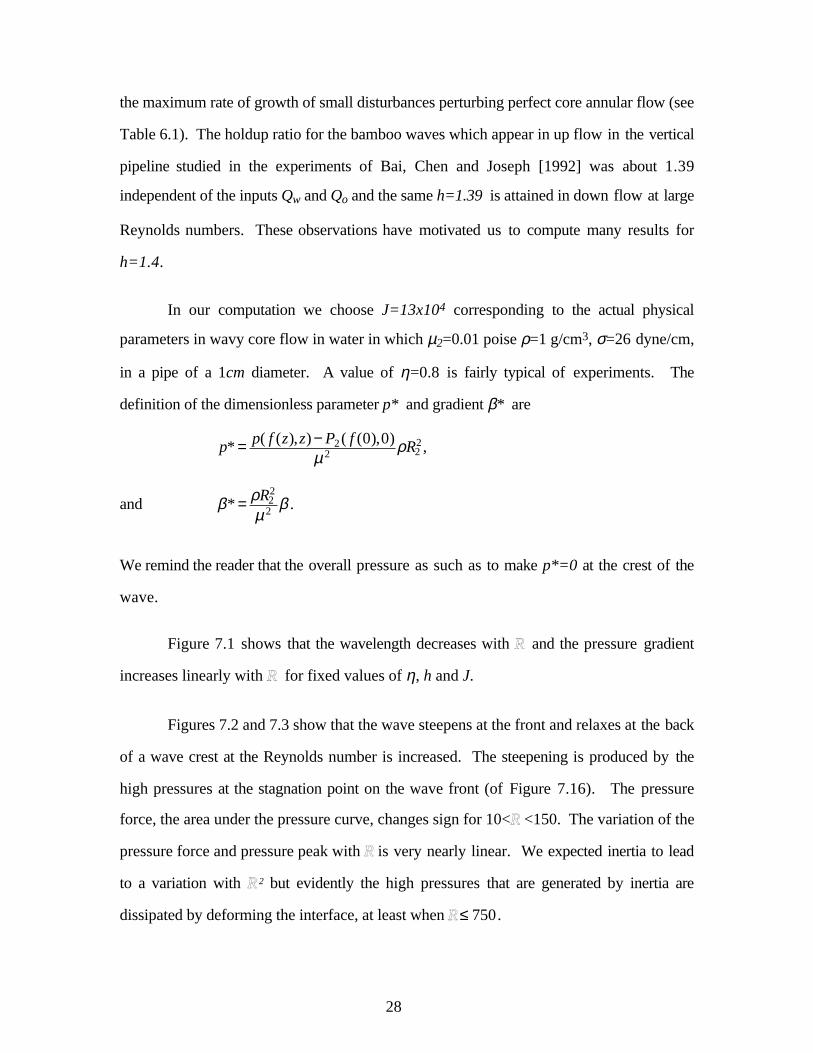
Figure 7.1 shows that the wavelength decreases with R and the pressure gradient
increases linearly with R for fixed values of η, h and J.
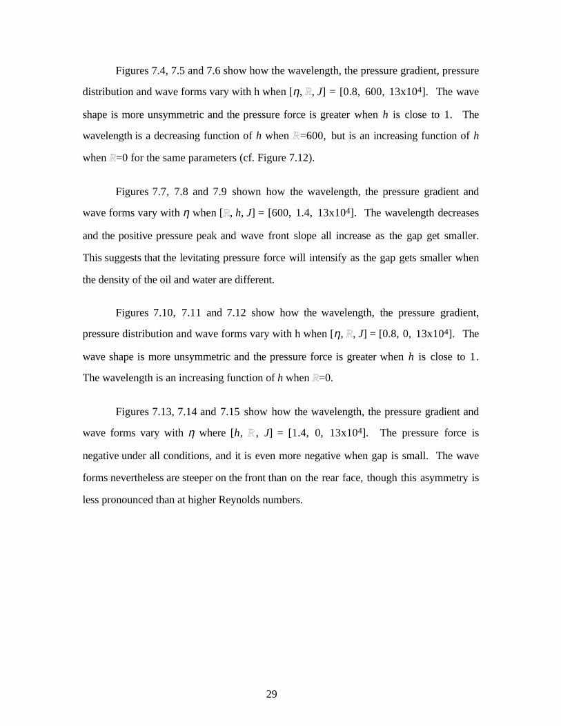
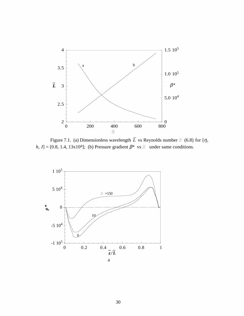
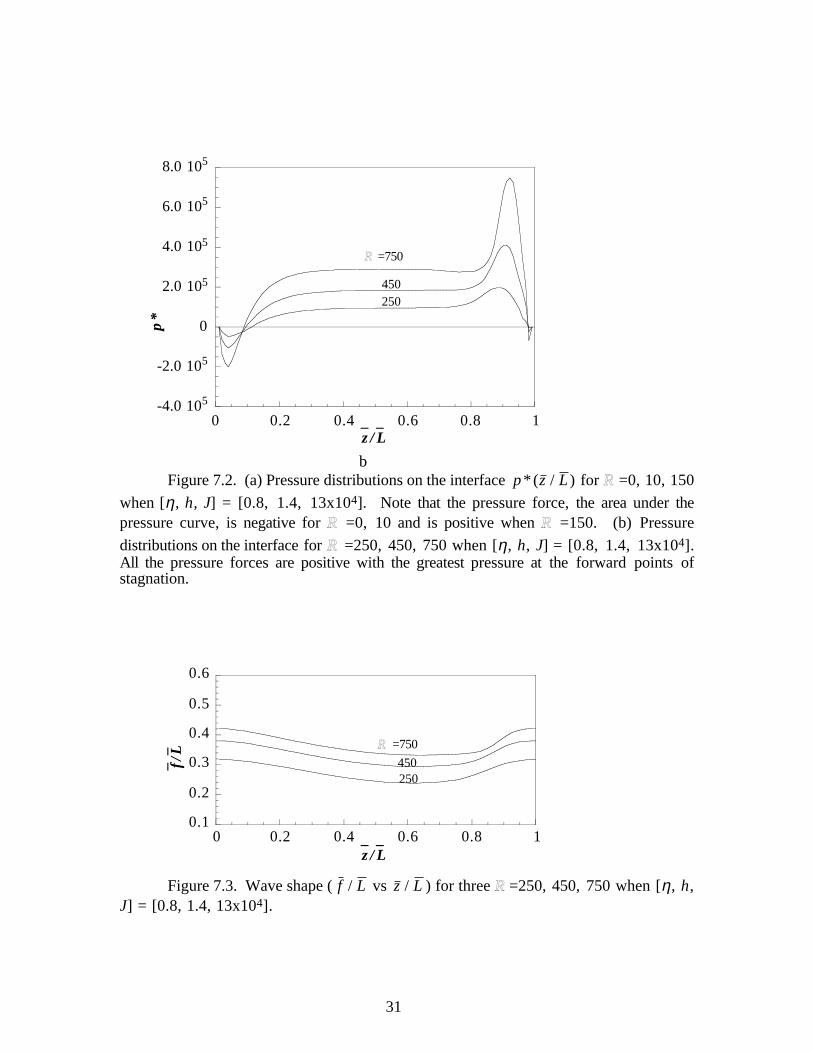
Figures 7.2 and 7.3 show that the wave steepens at the front and relaxes at the back
of a wave crest at the Reynolds number is increased. The steepening is produced by the
high pressures at the stagnation point on the wave front (of Figure 7.16). The pressure
force, the area under the pressure curve, changes sign for 10<R <150. The variation of the
pressure force and pressure peak with R is very nearly linear. We expected inertia to lead
to a variation with R 2 but evidently the high pressures that are generated by inertia are
dissipated by deforming the interface, at least when R≤ 750 .
29
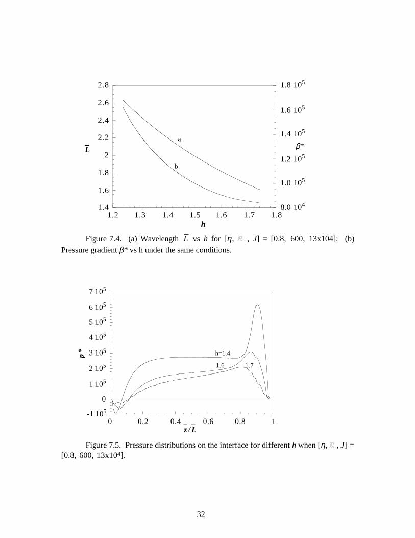
Figures 7.4, 7.5 and 7.6 show how the wavelength, the pressure gradient, pressure
distribution and wave forms vary with h when [η, R, J] = [0.8, 600, 13x104]. The wave
shape is more unsymmetric and the pressure force is greater when h is close to 1. The
wavelength is a decreasing function of h when R=600, but is an increasing function of h
when R=0 for the same parameters (cf. Figure 7.12).
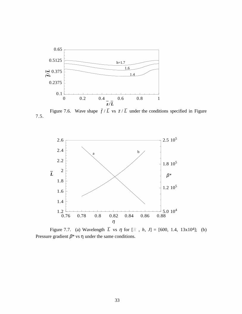
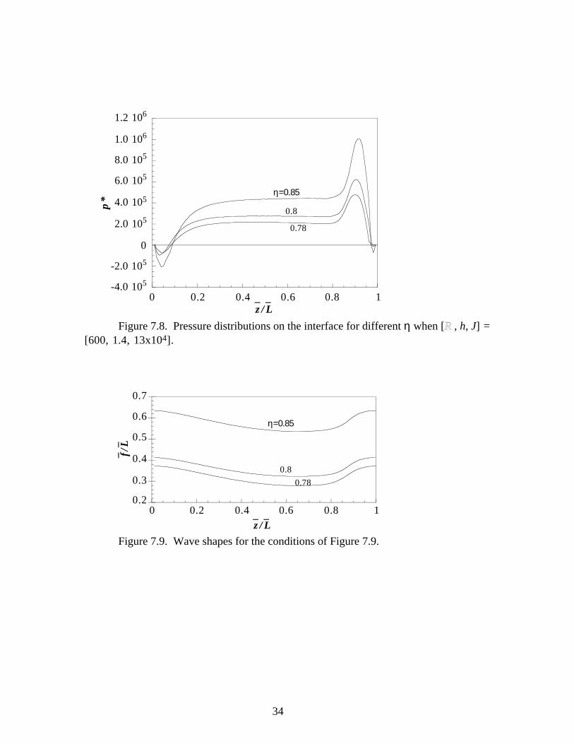
Figures 7.7, 7.8 and 7.9 shown how the wavelength, the pressure gradient and
wave forms vary with η when [R, h, J] = [600, 1.4, 13x104]. The wavelength decreases
and the positive pressure peak and wave front slope all increase as the gap get smaller.
This suggests that the levitating pressure force will intensify as the gap gets smaller when
the density of the oil and water are different.
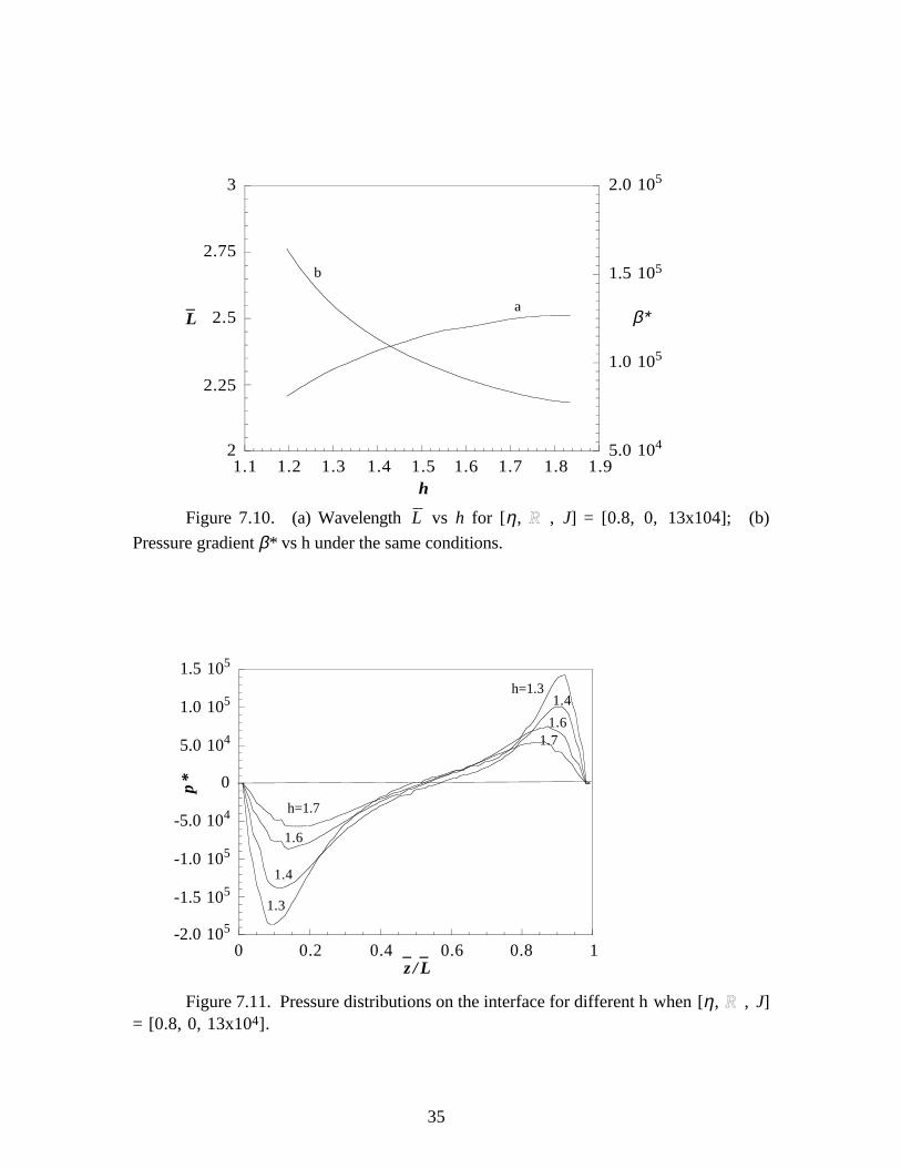
Figures 7.10, 7.11 and 7.12 show how the wavelength, the pressure gradient,
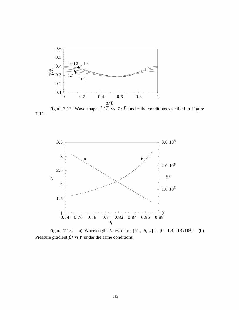
pressure distribution and wave forms vary with h when [η, R, J] = [0.8, 0, 13x104]. The
wave shape is more unsymmetric and the pressure force is greater when h is close to 1.
The wavelength is an increasing function of h when R=0.
Figures 7.13, 7.14 and 7.15 show how the wavelength, the pressure gradient and
wave forms vary with η where [h, R , J] = [1.4, 0, 13x104]. The pressure force is
negative under all conditions, and it is even more negative when gap is small. The wave
forms nevertheless are steeper on the front than on the rear face, though this asymmetry is
less pronounced than at higher Reynolds numbers.
30
2
2.5
3
3.5
4
_L β∗
0
5.0 104
1.0 105
1.5 105
0 200 400 600 800R
a b
Figure 7.1. (a) Dimensionless wavelength L vs Reynolds number R (6.8) for [η ,
h, J] = [0.8, 1.4, 13x104]; (b) Pressure gradient β* vs R under same conditions.
-1 105
-5 104
0
5 104
1 105
0 0.2
p*
0.4 0.6 0.8 1_ _z / L
R =150
10
0
a
31
-4.0 105
-2.0 105
0
2.0 105
4.0 105
6.0 105
8.0 105p
*
0 0.2 0.4 0.6 0.8 1_ _z / L
R =750
450250
bFigure 7.2. (a) Pressure distributions on the interface p *(z / L ) for R =0, 10, 150
when [η, h, J] = [0.8, 1.4, 13x104]. Note that the pressure force, the area under thepressure curve, is negative for R =0, 10 and is positive when R =150. (b) Pressure
distributions on the interface for R =250, 450, 750 when [η, h, J] = [0.8, 1.4, 13x104].All the pressure forces are positive with the greatest pressure at the forward points ofstagnation.
0.1
0.2
0.3
0.4
0.5
0.6
_ _
f/L
0 0.2 0.4 0.6 0.8 1_ _z / L
R =750
450250
Figure 7.3. Wave shape ( f / L vs z / L ) for three R =250, 450, 750 when [η, h,J] = [0.8, 1.4, 13x104].
32
1.4
1.6
1.8
2
2.2
2.4
2.6
2.8
_L β∗
8.0 104
1.0 105
1.2 105
1.4 105
1.6 105
1.8 105
1.2 1.3 1.4 1.5 1.6 1.7 1.8h
a
b
Figure 7.4. (a) Wavelength L vs h for [η, R , J] = [0.8, 600, 13x104]; (b)
Pressure gradient β* vs h under the same conditions.
-1 105
0
1 105
2 105
3 105
4 105
5 105
6 105
7 105
p*
0 0.2 0.4 0.6 0.8 1_ _z / L
h=1.4
1.6 1.7
Figure 7.5. Pressure distributions on the interface for different h when [η, R , J] =[0.8, 600, 13x104].
33
0.1
0.2375
0.375
0.5125
0.65
0
_ _
f/L
0.2 0.4 0.6 0.8 1_ _z / L
h=1.7
1.6
1.4
Figure 7.6. Wave shape f / L vs z / L under the conditions specified in Figure7.5.
1.2
1.4
1.6
1.8
2
2.2
2.4
2.6
_L β∗
5.0 104
1.2 105
1.8 105
2.5 105
0.76 0.78 0.8 0.82 0.84 0.86 0.88
a b
η
Figure 7.7. (a) Wavelength L vs η for [R , h, J] = [600, 1.4, 13x104]; (b)
Pressure gradient β* vs η under the same conditions.
34
-4.0 105
-2.0 105
0
2.0 105
4.0 105
6.0 105
8.0 105
1.0 106
1.2 106p
*
0 0.2 0.4 0.6 0.8 1_ _z / L
η=0.85
0.8
0.78
Figure 7.8. Pressure distributions on the interface for different η when [R , h, J] =[600, 1.4, 13x104].
0.2
0.3
0.4
0.5
0.6
0.7
0 0.2 0.4
_ _
f/L
0.6 0.8 1_ _z / L
η=0.85
0.8
0.78
Figure 7.9. Wave shapes for the conditions of Figure 7.9.
35
2
2.25
2.5
2.75
3
5.0 104
1.0 105
1.5 105
_L β∗
2.0 105
1.1 1.2 1.3 1.4 1.5 1.6 1.7 1.8 1.9
a
b
h
Figure 7.10. (a) Wavelength L vs h for [η, R , J] = [0.8, 0, 13x104]; (b)
Pressure gradient β* vs h under the same conditions.
-2.0 105
-1.5 105
-1.0 105
-5.0 104
0
5.0 104
1.0 105
1.5 105
p*
0 0.2 0.4 0.6 0.8 1_ _z / L
h=1.7
h=1.31.4
1.6
1.7
1.3
1.6
1.4
Figure 7.11. Pressure distributions on the interface for different h when [η, R , J]= [0.8, 0, 13x104].
36
0.1
0.2
0.3
0.4
0.5
0.6
0 0.2
_ _
f/L
0.4 0.6 0.8 1
h=1.3 1.4
_ _z / L
1.61.7
Figure 7.12 Wave shape f / L vs z / L under the conditions specified in Figure7.11.
1
1.5
2
2.5
3
3.5
_L β∗
0
1.0 105
2.0 105
3.0 105
0.74 0.76 0.78 0.8 0.82 0.84 0.86 0.88
a b
η
Figure 7.13. (a) Wavelength L vs η for [R , h, J] = [0, 1.4, 13x104]; (b)
Pressure gradient β* vs η under the same conditions.
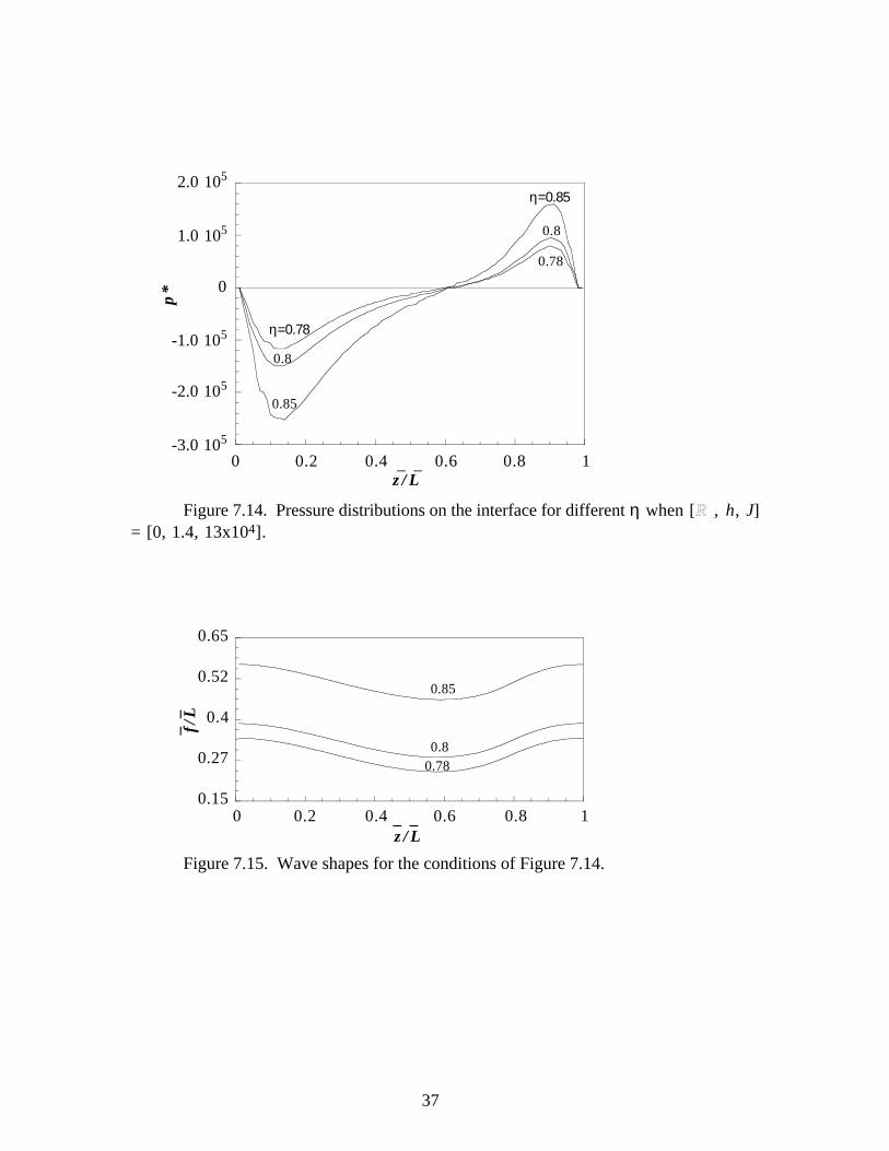
37
-3.0 105
-2.0 105
-1.0 105
0
1.0 105
2.0 105p
*
0 0.2 0.4 0.6 0.8 1z / L
η=0.78
0.8
0.85
_ _
η=0.85
0.8
0.78
Figure 7.14. Pressure distributions on the interface for different η when [R , h, J]= [0, 1.4, 13x104].
0.15
0.27
0.4
0.52
0.65
0 0.2 0.4 0.6
_ _
f/L
0.8 1
0.780.8
_ _z / L
0.85
Figure 7.15. Wave shapes for the conditions of Figure 7.14.

38
39
a
b
c
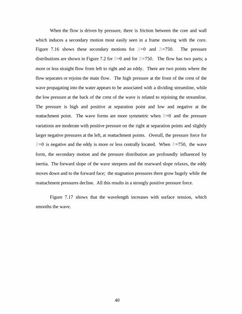
dFigure 7.16. Secondary motions for (a) [R , η , h, J] = [0, 0.8, 1.4, 13x104], (b)
[R, η , h, J] = [750, 0.8, 1.4, 13x104]; The pressure at the stagnation point on the steepslope at the right corresponds to the pressure maximum shown in Figure 7.2(b), (c) theeddies for Stokes flow as the same condition of (a), (d) the eddies as the same condition of(b).
40
When the flow is driven by pressure, there is friction between the core and wall
which induces a secondary motion most easily seen in a frame moving with the core.
Figure 7.16 shows these secondary motions for R=0 and R=750. The pressure
distributions are shown in Figure 7.2 for R=0 and for R=750. The flow has two parts; a
more or less straight flow from left to right and an eddy. There are two points where the
flow separates or rejoins the main flow. The high pressure at the front of the crest of the
wave propagating into the water appears to be associated with a dividing streamline, while
the low pressure at the back of the crest of the wave is related to rejoining the streamline.
The pressure is high and positive at separation point and low and negative at the
reattachment point. The wave forms are more symmetric when R=0 and the pressure
variations are moderate with positive pressure on the right at separation points and slightly
larger negative pressures at the left, at reattachment points. Overall, the pressure force for
R=0 is negative and the eddy is more or less centrally located. When R=750, the wave
form, the secondary motion and the pressure distribution are profoundly influenced by
inertia. The forward slope of the wave steepens and the rearward slope relaxes, the eddy
moves down and to the forward face; the stagnation pressures there grow hugely while the
reattachment pressures decline. All this results in a strongly positive pressure force.
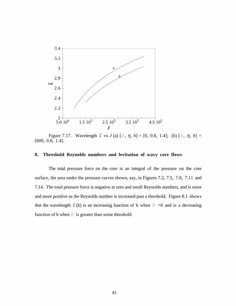
Figure 7.17 shows that the wavelength increases with surface tension, which
smooths the wave.
41
2
2.2
2.4
2.6
2.8
3
3.2
_ L3.4
5.0 104 1.5 105 2.5 105 3.5 105 4.5 105
a
b
J
Figure 7.17. Wavelength L vs J (a) [R , η , h] = [0, 0.8, 1.4]; (b) [R , η , h] =[600, 0.8, 1.4].
8. Threshold Reynolds numbers and levitation of wavy core flows
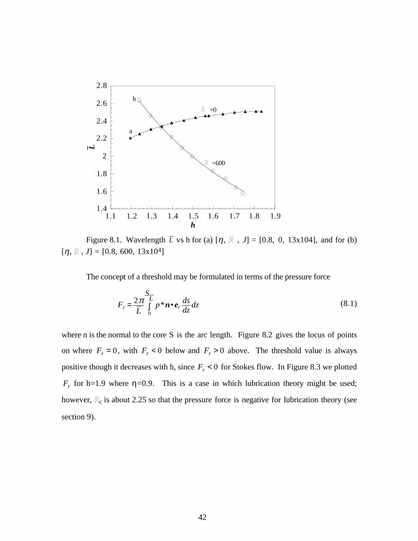
The total pressure force on the core is an integral of the pressure on the core
surface, the area under the pressure curves shown, say, in Figures 7.2, 7.5, 7.8, 7.11 and
7.14. The total pressure force is negative at zero and small Reynolds numbers, and is more
and more positive as the Reynolds number is increased past a threshold. Figure 8.1 shows
that the wavelength L (h) is an increasing function of h when R =0 and is a decreasing
function of h when R is greater than some threshold.
42
1.4
1.6
1.8
2
2.2
2.4
2.6
2.8_ L
1.1 1.2 1.3 1.4 1.5 1.6 1.7 1.8 1.9h
R
R
=600
=0
b
a
Figure 8.1. Wavelength L vs h for (a) [η, R , J] = [0.8, 0, 13x104], and for (b)
[η , R , J] = [0.8, 600, 13x104]
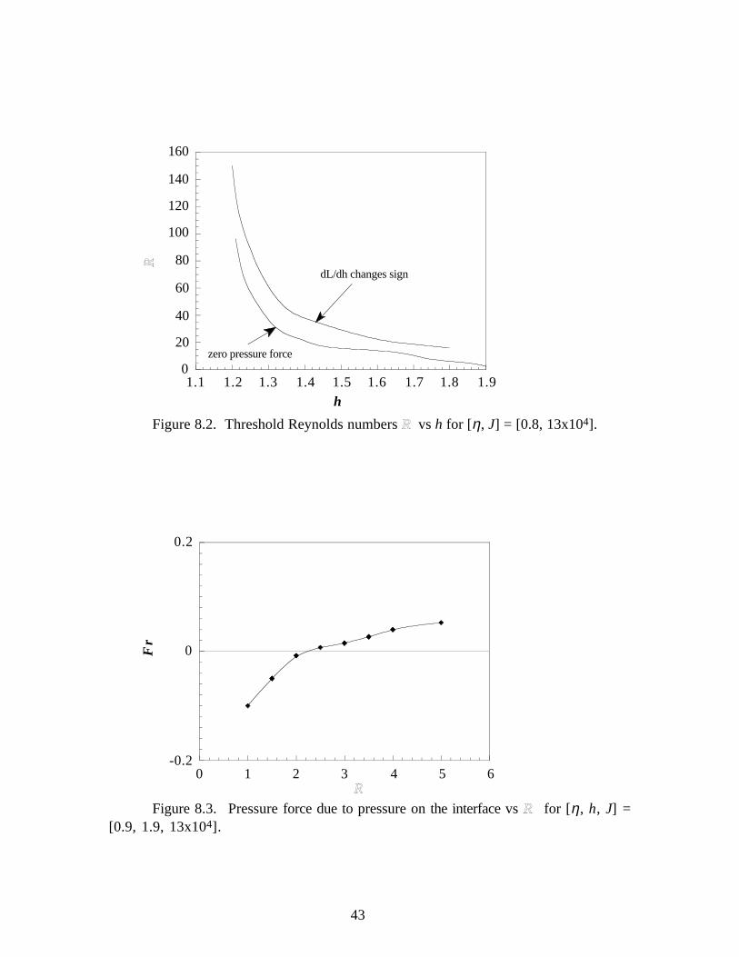
The concept of a threshold may be formulated in terms of the pressure force
Fr = 2πL
p*n•erdsdz
dz0
SL∫ (8.1)
where n is the normal to the core S is the arc length. Figure 8.2 gives the locus of points
on where Fr = 0 , with Fr < 0 below and Fr > 0 above. The threshold value is always
positive though it decreases with h, since Fr < 0 for Stokes flow. In Figure 8.3 we plotted
Fr for h=1.9 where η=0.9. This is a case in which lubrication theory might be used;
however, Rc is about 2.25 so that the pressure force is negative for lubrication theory (see
section 9).
43
0
20
40
60
80
100
120
140
160R
1.1 1.2 1.3 1.4 1.5 1.6h
1.7 1.8 1.9
zero pressure force
dL/dh changes sign
Figure 8.2. Threshold Reynolds numbers R vs h for [η, J] = [0.8, 13x104].
-0.2
0
0.2
0 1 2
Fr
3 4 5 6R
Figure 8.3. Pressure force due to pressure on the interface vs R for [η, h, J] =[0.9, 1.9, 13x104].

44
3
3.2
3.4
3.6
3.8
4
1.1 1.2
_ L
1.3 1.4 1.5 1.6 1.7h
Figure 8.4. The slope dL/dh of the wavelength changes with holdup ratio for [η ,R, J]=[0.8, 100, 13x104].
We may argue that a positive levitation of a lighter or a heavier than water core flow
requires a positive pressure force to push the core away from wall. The pressure forces are
associated with the form of waves that they generate. Waves also develop in Stokes flow,
but the pressure forces associated with these waves are negative like those on the reversed
slipper bearing which pull the slipper to the wall. When the Reynolds number is higher
than the threshold, high positive pressures are generated, especially at the stagnation point
on the steep part of the wave front (Figure 7.16).
In the axisymmetric problem with matched density considered here, lateral motions
of the core off center are not generated by pressure forces, whether they be positive or
negative, because the same pressure acts all around the core. We may consider what might
happen if the core moved to a slightly eccentric position due to a small difference in
density. The pressure distribution in the narrow part of gap would intensify and the
pressure in the wide part of the gap would relax according to the predicted variation of
45
pressure with η shown in Figure 7.8. In this case a more positive pressure would be
generated in the narrow gap which would levitate the core. The equilibrium position of the
core would then be determined by a balance between buoyancy and levitation by pressure
forces which, in the case of matched densities, would center the core. In eccentric
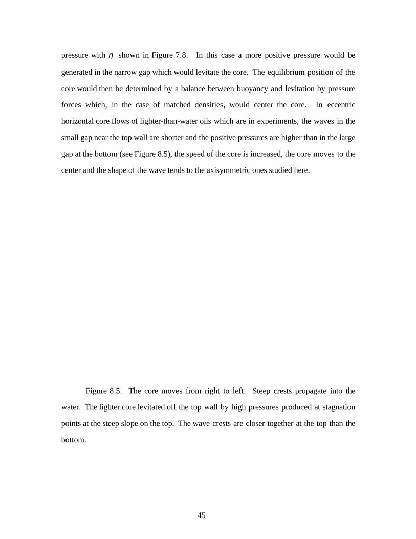
horizontal core flows of lighter-than-water oils which are in experiments, the waves in the
small gap near the top wall are shorter and the positive pressures are higher than in the large
gap at the bottom (see Figure 8.5), the speed of the core is increased, the core moves to the
center and the shape of the wave tends to the axisymmetric ones studied here.
Figure 8.5. The core moves from right to left. Steep crests propagate into the
water. The lighter core levitated off the top wall by high pressures produced at stagnation
points at the steep slope on the top. The wave crests are closer together at the top than the
bottom.
46
9. Lubrication theory
Lubrication theory is valid when inertia is neglected (Stokes flow), when the wave
amplitude is small and the radial velocity u and ∂w ∂z are negligible. The last conditions
imply that secondary motions are not present or are very weak. The required conditions
can be achieved in the limit in which R and 2-h tend to zero, in Stokes flows which perturb
perfect core flows. Small gaps are one way to achieve small R , but other possibilities are
compatible with lubrication theory. It is of value to examine the lubrication theory in bright
light since it is very popular with applied mathematicians and has played an historically
important role in the development of the theory of core flows.
After applying the assumptions of lubrication theory, the governing equations
(3.11) reduce to
0 = β − ∂p
∂z+ µ2
1r
∂∂r
r∂w
∂r
. (9.1)
where w=0 at r=f(z) and w=-c at r=R2. Hence
w(r) = 14µ
dP2
dz(r2 − f 2 (z)) −
c + 14µ
dP2
dz(R2 − f 2 (z))
lnR2
f
lnr
f
, (9.2)
where P2 = −βz + p(z) + P2 (0) , (9.3)
and P2 (0) − P2 (L)
L= β . (9.4)
The pressure difference is opposed by the integral of the shear stress on the wall,
βL • πR22 = 2πR2 µ2
dw(r)dr
0
L
∫ r = R2dx (9.5)
After combining (9.2) and (9.5), we relate the wave speed c to the pressure gradient
47
c = − 14µ2
dP
dz(R2
2 − f 2 ). (9.6)
This equation can be also obtained from (4.5) with µ1 → ∞ . For a given speed c, the
pressure gradient is determined by the shape of the core.
dP2
dz= −β + dp
dz= − 4µc
R22 − f 2 (z) . (9.7)
Since p is a periodic function, the driving pressure gradient is given by
β = P2 (0) − P2 (L)L
= 1L
4µc
R22 − f 2 (z)
dz0
L
∫ . (9.8)
The periodic pressure, a functional of f(z), is
p(z) − P2 (0) = βz − 4µc
R22 − f 2 (z)
dz0
z
∫ . (9.9)
In the perfect core annular flow f(z)=R1 is uniform and (9.8) and (9.9) show that p(z)-
P2(0)=0 and pressure gradient will be constant.
We carried out an analysis of these equation by assuming f(z) and computing p(z).
Of course, the normal stress balance is not satisfied by the assumed shape but we could
iterate all of the assumed shapes to a unique one which satisfies the reduced normal stress
balance (3.12)
P1 − P2 = σf 1 + f ' 2
− σf "(1 + f ' 2 )3/ 2 . (9.10)
Here
P1 = −βz + P1(0) (9.11)
in the core and (9.7) implies that
P2 = − 4µc
R22 − f 2 (z)
dz0
x
∫ − P2 (0) (9.12)
48
in the annulus. The pressure jump across the interface is then
P1 − P2 = −βz + 4µ2c
R22 − f 2 (z)
0
z
∫ dz + Cp , (9.13)
where Cp = P1(0) − P2 (0) .
Our iteration starts with any trial wave, say f1(z). Then we compute
P1 − P2 = −βz + 4µ2c
R22 − f1
2 (z)0
z
∫ dz + Cp
and carry out the first iteration using the normal stress balance to compute f2(z):
−βz + 4µ2c
R22 − f1
2 (z)0
z
∫ dz + Cp = σf 2 1 + f 2'
2− σf 2"
(1 + f 2'2 )3/ 2
.
We then compute
P1 − P2 = −βz + 4µ2c
R22 − f 2
2 (z)0
z
∫ dz + Cp
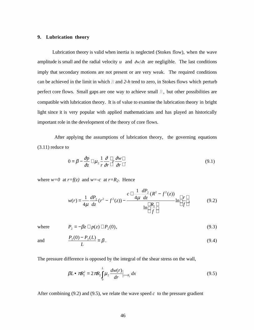
and so on. This iteration converges to the unique solution shown in Figure 9.1 for each of
three very different guesses for f1(z).
0.7
0.75
0.8
0.85_ _
f/L
p*0.9
0.95
1
-2.0 104
-1.5 104
-1.0 104
-5.0 103
0
5.0 103
1.0 104
_ _z / L
0 0.2 0.4 0.6 0.8 1
Figure 9.1. Pressure distribution and wave shape from lubrication theorywhen [η, h, J]= [0.8, 1.9, 13x104].
49
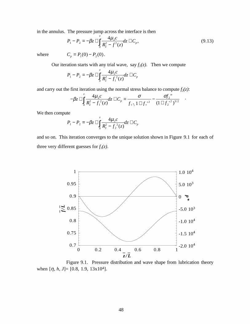
The wave is nearly symmetric, but the pressure force is slightly negative. Figure
9.2 compares the pressure distribution from lubrication theory and Stokes flow; in both
cases the area under the pressure curve is negative. To use lubrication theory as a
predictive tool, it is necessary at least to study the stability of the flow with h near 2, in
most cases they will be unstable. Stable flows may be unstable to off-center perturbations
of the type considered by Huang and Joseph [1994] at small but finite Reynolds numbers
since the unbalanced core could possibly be sucked to the wall by the negative pressure
force.
-1.000 104
0
1.000 104
0 0.5 1
lubrication theory
p*
Stokes flow
_ _z / L
Figure 9.2. Comparison of pressure distributions when [η, h, J]= [0.8, 1.9,13x104].
10. Conclusions
Core annular flows of liquids with the same density and a high viscosity ratio were
computed in a direct numerical simulation. It was assumed that flow is axisymmetric and
the core is solid with adveceted periodic standing interfacial waves fixed on the moving
core. These assumptions reduce the number of parameters defining the problem to four :
50
Reynolds number, radius ratio, holdup ratio and surface tension parameter. In dimensional
terms, for given material parameters, we get solutions when the volume flow rates of oil,
water and the holdup ratio are prescribed. Only the flow rates are given in experiments and
the holdup is then determined by stability, so we are computing a family of the solutions
most of which are unstable.
The numerical solutions have the properties predicted by Joseph in Feng et al. ; the
high pressures on the forward facing slope of the wave, where the water enters into a
converging gap, steepen the wave and reduction of the pressure on the lee side smooths the
wave. This leads to unsymmetric waves unlike those which levitate a slipper bearing. The
problem of levitation does not arise in the density matched core, but the pressure
distributions which actually develop in this case seem to be such as to center a slightly
displaced core only when the Reynolds number is greater than a threshold value which
depends on the parameters but in all cases is strictly positive. Levitation of core flow by
inertia is a new and potentially interesting idea which has been given an explicit predictable
form by the analysis of this paper.
Acknowledgments
This work was supported by the Department of Energy, Office of Basic Energy
Science; the National Science Foundation; and the Minnesota Supercomputer Institute. The
authors wish to thank Mr. J. Feng, Adam Huang, Peter Huang, Terrence Liao and Walter
Wang for their help and helpful discussions.
Appendix – Computational Solution of the Core Annular Flow
The axisymmetric core annular flow with the deformable oil core is governed by
Eq. (3.11) subject to the normal stress condition specified in Eq. (3.12) and the force
balance on the oil core described in Eq. (3.14). For each given value of the parameter triplet
(c, R1, h), computational solution of these equation is carried out to determine the flow of
51
water, the shape and location of the free surface of the oil core, and the wavelength. This
calculation involves an iterative solution between the calculation of the flow filed of water
and the calculation of the free surface shape. In the following discussion, important details
of these two steps and the overall solution algorithm are described.
Computation of the Flow Field of Water
The velocity and the pressure field involve solution of momentum and continuity
equation (Eq. (3.11)) for the specified wave speed c and the available free surface shape
and wavelength. Relevant details of the discretization method and the solution technique
and the procedure for the determination of the pressure gradient β are now described.
Discretization Method and Solution Technique – The control volume based
computational method of Patankar (1980) is used for the solution of the Navier-Stokes
equations governing the flow of water. In this method, the domain of interest is divided
into a set of control volumes. Values of scalar unknowns including pressure are stored at
the main grid points. A staggered grid is used for storing the velocity components to avoid
the occurrence of checker boarding of the pressure field. Thus, a normal velocity
component is stored on each control volume face. This gives rise to momentum control
volumes in the z- or r-directions to be displaced in the z- or r-directions respectively. The
discretization equations for z- or r-direction velocity components are constructed by
integrating the z- and r-direction momentum equations over the control volumes staggered
in z- and r-directions respectively. The continuity equation is discretized over the main
control volume. The convective-diffusive fluxes over the control volume faces are
computed using the Power-law scheme (Patankar, 1980). The resulting discretization
method expresses perfect conservation over individual control volumes and the entire
domain.
52
Two important issues need to be addressed in the application of this discretization
method for predicting the flow field of water – the representation of the free surface and the
treatment of the periodicity conditions. In the present study, an axisymmetric cylindrical
grid is used to discretize the entire domain (0 ≤ r ≤ R2, 0 ≤ x ≤ L). The rigid core is
represented by imposing a zero velocity on the control volumes that lie in the oil core
through the use of a high viscosity. This procedure approximates the wavy interface using
a stepped grid. A grid independence study was carried out to determine the size of the grid
necessary for accurate prediction of the water flow and the interface shape using increase
number of grid points until the accuracy of the pressure distribution no significant change.
The prediction of the core annular flow is carried assuming that the deformation of the
wavy interface is spatially periodic. This enables prediction of flow over segment of the
pipe corresponding to one wavelength. Thus, all variables in Eq. (3.11) are periodic at z =
0 and L. During discretization, the control volume faces at z = 0 and L are treated as
topologically coincident to incorporate this periodicity condition (Patankar, Liu, and
Sparrow, 1977).
The discretized momentum and continuity equations are solved using the SIMPLER
algorithm (Patankar, 1980) that addresses the velocity-pressure coupling effectively. The
algorithm involves sequential solution of the pressure, momentum, and pressure-correction
equations. The line-by-line method is used for the solution of the discretization equations
for each variable. The circular Tri-Diagonal-Matrix-Algorithm (TDMA) is used for solution
of the discretization equations along lines in the periodic direction.
Determination of the Pressure Gradient β – Since we have chosen to
specify the wave speed c, the corresponding pressure gradient β in Eq. (3.11) has to be
calculated. The condition of force balance on the oil core expressed in Eq. (3.14) provides
a natural method for its determination. Thus, in each iteration of the SIMPLER procedure
for calculating the water flow field, the value of β is updated according to Eq. (3.14) based
53
on the available pressure P2 and the shear stress τ on the free surface of the oil core. At
convergence of the internal iterations for the calculation of the water flow field, the value of
β is determined for the specified wave speed c and the available free surface shape.
Determination of the Free Surface Shape
Computational prediction of the free surface shape involves discretization and
solution of the normal stress equation with an iterative adjustment of the surface shape for
obtaining the prescribed average core radius R1 and the holdup ratio h. Important details of
these steps are now described.
Discretization and Solution of the Normal Stress Condition – The shape
of the interface is governed by the normal stress and pressure jump condition reproduced
below.
d 2 f
dz2 −1 + df
dz
2
f+ 1
σ1 + df
dz
2
3
2
Cp − p(z)( ) = 0 (A.1)
The solution of this equation is sought for the available pressure variation p(z) on the free
surface that is determined from calculation of the water flow field. The unknown shape f(z)
is represented by discrete values of f at the same locations in z-direction used in the
calculation of the flow field of water. The equations for these values of f(z) are constructed
by integrating the above equation over the main control volumes in the z-direction. The last
term in the equation is treated explicitly as a source term and is assumed to be constant over
the control volume. The resulting discretization equation has the following form.

54
ai f i = bi f i+1 + ci f i−1 + S∆zi (A.2)
where bi = 1zi+1 − zi
, ci = 1zi − zi−1
, ai = bi + ci +1 + df *i
dz
2
f *i2
∆zi ,
Si = 1σ
1 + df *i
dz
2
3
2
Cp − pi **( ),
and ∆zi = (zi+1 − zi−1) 2 .
Similar to the flow field calculation, the periodicity of fi values is accounted for in the
above equations by recognizing that in the equation for fN, the fi+1 is replace by f1 while in
the equations for f1, the fi-1 is replaced by fN. The single * in Eq. (A.2) represent available
values that are updated within the inner iteration for determining the free surface shape
while the **s on pi denote that these values are kept constant during the free surface
calculation and updated only in the outer iteration.
Adjustment for Fixed R1 and h – The unknown pressure jump Cp and the
wavelength L provide the two degrees of freedom necessary to determine the free surface
shape consistent with the specified values of the average plug radius R1 and the holdup
ratio h. After each iteration during calculation of the fi values, the value of Cp is increased
or decreased according to whether the available fi values imply a value of R1 larger or
smaller than that desired. Similarly, the wavelength L is increased or decreased if the
current value of the holdup ratio h is larger or smaller than its prescribed value. The amount
of adjustment in the values of Cp and L is determined using the secant method. It uses the
predictions from the last two iterations to determine the sensitivity of R1 and h to changes
in Cp and L. The sensitivity coefficients are then used for inferring the changes in Cp and L
to be made in the next iteration. At convergence, this procedure provides a free surface
shape and location having the desired R1 and h for the surface pressure variation
determined from the flow field calculation.
55
Overall Solution Algorithm
The overall solution method involves an outer iteration between the flow field
calculation for water and the determination of the free surface and is outlined below.
1. Prescribe the values of wave speed c, average core radius R1, and the holdup ratio h.
2. Assume a free surface shape. Calculate the velocity and pressure fields in the water
region for the specified wave speed c. During each iteration of the flow field calculation,
the pressure gradient β is adjusted to satisfy the force balance on the oil plug.
3. The shape of the free surface is determined by solving the equation describing the
normal stress condition for the surface pressure determined from step 2. The wavelength
and the pressure jump are adjusted in each iteration so that at convergence the free surface
shape is determined for the prescribed average core radius R1 and holdup ratio h.
4. The new free surface is now used in determining the flow field in step 2. Thus, steps 2
and 3 are repeated till convergence to obtain a self-consistent flow field of water and free
surface shape of the oil core for the prescribed values of the parameter triplet (c, R1, h).
The overall solution method correctly predicted the perfect core flow. Further, it
predicted the same free surface shape in the flow field of water irrespective of the initial
guess surface. This constituted a rigorous test for the correctness of the computational
technique. Consequently, the above method was applied for computing the details of the
wavy core flow for a range of the parameter triplet (c, R1, h).
Reference
Bai, R., Chen, K., Joseph, D. D. 1992 Lubricated pipelining: Stability of core-annular
flow. Part 5: Experiments and comparison with theory. J. Fluid Mech. 240, (1992), 97-
142.
56
Charles, M. E. 1963 The pipeline flow of capsules. Part 2: theoretical analysis of the
concentric flow of cylindrical forms. Can. J. Chem. Engng. April 1963, 46
Charles, M. E. Govier, G. W. & Hodgson, G. W. 1961 The horizontal pipeline flow of
equal density of oil-water mixtures. Can. J. Chem. Engng. 39, 17-36
Chen, K. , Bai, R. & Joseph, D. D. 1990 Lubricated pipelining. Part 3. Stability of core-
annular flow in vertical pipes. J. Fluid Mech. 214, 251-286
Chen, K. & Joseph, D. D. 1990 Lubricated pipelining: stability of core-annular flow. Part
4. Ginzburg-Landau equations. J. Fluid Mech. 227, 226-260
Feng, J., Huang, P. Y., Joseph, D. D. 1995 Daynamic simulation of the motion of capsuls
in pipelines. J. Fluid Mech. 286, 201-227
Hasson, D. Mann, U. & Nir, A. 1970 Annular flow of two immiscible liquids. I.
Mechanisms. Can. J. Chem. Engng. 48, 514
Hu, H. & Joseph, D. D. 1989a Lubricated pipelining: stability of core-annular flow. Part
2. J. Fluid Mech. 205, 359-396
Hu, H. & Joseph, D. D. 1989b Stability of core-annular flow in a rotating pipe. Phys.
Fluids A1(10), 1677-1685
Huang, A. & Joseph, D. D. 1995 Stability of eccentric core annular flow. J. Fluid
Mech. 282, 233-245
Joseph, D. D., Nguyen, K. & Beavers, G. S. 1984 Non-uniqueness and stability of the
configuration of flow of immiscible fluids with different viscosities. J. Fluid Mech. 141 ,
319-345
57
Joseph, D. D., Renardy, Y. Y. 1993 Fundamentals of two-fluid dynamics. Spring-Verlag
New York, Inc.
Joseph, D. D., Renardy, Y. & Renardy, M. 1984 Instability of the flow of immiscible
liquids with different viscosities in a pipe. J. Fluid Mech. 141, 309-317
Joseph, D. D., Singh, P. & Chen, K. 1989 Couette flows, rollers, emulsions, tall Taylor
cells, phase separation and inversion, and a chaotic bubble in Taylor-Couette flow of two
immiscible liquids. in Nonlinear Evolution of Spatio-temporal Structures in
Dissipative Continuous Systems (ed. F. H. Busse & L. Kramer), Plenum Press, New
York. (in the press).
Liu, H 1982 A theory of capsule lift-off in pipeline. J. Pipelines 2, 23-33
Oliemans, R. V. A. 1986 The lubricating film model for core-annular flow. Delft
University Press. [(v1) 5, 338; (v2) 1, 195-196, 200]
Oliemans, R. V. A. & Ooms, G. 1986 Core-annular flow of oil and water through a
pipeline. Multiphase Science and Technology. 2, eds. Hewitt, G. F., Delhaye, J. M. &
Zuber, N., Hemisphere Publishing Corporation. [(v1) 4, 5; (v2) 1, 19]
Ooms, G., Segal, A., Van der Wees, A. J., Meerhoff, R. & Oliemans, R. V. A. 1984 A
theoretical model for core-annular flow of a very viscous oil core and a water annulus
through a horizontal pipe. Int. J. Multiphase Flow 10, 41. [(v1) 338; (v2) 10]
Patankar, S. V., Liu, C. H., & Sparrow, E. M. 1977 Fully developed flow and heat
transfer in ducts having streamwise-periodic variations of cross-section area. J.Heat
transfer. 99, 180.
Preziosi, L. Chen, K. & Joseph, D. D. 1989 Lubricated pipelining: stability of core-
annular flow. J. Fluid Mech. 201, 323-356
58
Russell, T. W. F. & Charles, M. E. 1959 The effect of the less viscous liquid in the
laminar flow of two immiscible liquids. Can. J. Chem. Engng. 39, 18-24
Than, P., Rosso, F. & Joseph, D. D. 1987 Instability of Poiseuille flow of two
immiscible liquids with different viscosities in a channel. Int. J. Engng. Sci. 25, 189
Tipman, E. & Hodgson, G. W. 1956 Sedimentation in emulsions of water in petroleum.
J. Petroleum Tech. September, 91-93