Rochester Institute of Technology Rochester Institute of Technology

RIT Scholar Works RIT Scholar Works

Theses

1-2014

Design for Implementation of Image Processing Algorithms Design for Implementation of Image Processing Algorithms

Jamison D. Whitesell

Follow this and additional works at: https://scholarworks.rit.edu/theses

Recommended Citation Recommended Citation Whitesell, Jamison D., "Design for Implementation of Image Processing Algorithms" (2014). Thesis. Rochester Institute of Technology. Accessed from

This Thesis is brought to you for free and open access by RIT Scholar Works. It has been accepted for inclusion in Theses by an authorized administrator of RIT Scholar Works. For more information, please contact [email protected].

Design for Implementation of Image Processing Algorithms

by

Jamison D. Whitesell

A Thesis Submitted in Partial Fulfillment of the Requirements for the Degree of

Master of Science in Electrical Engineering

Supervised by

Dr. Dorin Patru

Department of Electrical and Microelectronic Engineering

Kate Gleason College of Engineering

Rochester Institute of Technology

Rochester, NY

January 2014

Approved By:

Dr. Dorin Patru

Associate Professor – R.I.T. Dept. of Electrical and Microelectronic Engineering

Dr. Eli Saber

Professor – R.I.T. Dept. of Electrical and Microelectronic Engineering

Dr. Mehran Kermani

Assistant Professor – R.I.T. Dept. of Electrical and Microelectronic Engineering

Dr. Sohail Dianat

Department Head – R.I.T. Dept. of Electrical and Microelectronic Engineering

ii

Dedication

To my family,

without whom none of my success would be possible.

iii

Acknowledgements

I would like to thank:

Dr. Dorin Patru for giving me the opportunity to be a part of this research and for

guidance throughout the thesis process;

Brad Larson, Gene Roylance, and Kurt Bengston for their insight and continued support;

Ryan Toukatly and Alex Mykyta for their research efforts which lay the technical

groundwork for this project;

James Mazza, Sankaranaryanan Primayanagam, and Osborn de Lima for providing

valuable suggestions during the course of this work;

and my committee members, Dr. Eli Saber and Dr. Mehran Kermani;

iv

Abstract

Color image processing algorithms are first developed using a high-level

mathematical modeling language. Current integrated development environments offer

libraries of intrinsic functions, which on one hand enable faster development, but on the

other hand hide the use of fundamental operations. The latter have to be detailed for an

efficient hardware and/or software physical implementation. Based on the experience

accumulated in the process of implementing a segmentation algorithm, this thesis outlines

a design for implementation methodology comprised of a development flow and associated

guidelines.

The methodology enables algorithm developers to iteratively optimize their

algorithms while maintaining the level of image integrity required by their application.

Furthermore, it does not require algorithm developers to change their current development

process. Rather, the design for implementation methodology is best suited for optimizing

a functionally correct algorithm, thus appending to an algorithm developer’s design process

of choice.

The application of this methodology to four segmentation algorithm steps produced

measured results with 2-D correlation coefficients (CORR2) better than 0.99, peak-signal-

to-noise-ratio (PSNR) better than 70 dB, and structural-similarity-index (SSIM) better than

0.98, for a majority of test cases.

v

Table of Contents

Dedication .......................................................................................................................... ii

Acknowledgements .......................................................................................................... iii

Abstract ............................................................................................................................. iv

Table of Contents ...............................................................................................................v

List of Figures .................................................................................................................. vii

List of Symbols ...................................................................................................................x

Glossary ........................................................................................................................... xii

Chapter 1: Introduction ..............................................................................................1

Chapter 2: Background ...............................................................................................5

2.1 Related Work .....................................................................................................5

2.2 Prior Research Leading to the Multichannel Framework ..................................8

2.3 The GSEG Algorithm as a Test Vehicle .........................................................10

Chapter 3: Algorithm Modifications........................................................................13

3.1 Design for Implementation Test Vehicle .........................................................13

3.2 Modifications to the MCF Instruction Set .......................................................20

Chapter 4: Design for Implementation ....................................................................24

4.1 Design for Implementation Flow .....................................................................24

4.2 Design for Implementation Guidelines ............................................................26

4.3 General Applicability of the Proposed Methodology ......................................29

Chapter 5: Implementation of the Test Vehicle ......................................................31

5.1 Conversions between Programming Languages ..............................................31

5.2 Image Quality Metrics and Validation ............................................................35

5.3 Test Setup ........................................................................................................38

vi

Chapter 6: Results and Discussions .........................................................................39

6.1 Validation of Algorithm Modifications ...........................................................39

6.2 Cases of Significant Degradation ....................................................................42

6.3 Logic Utilization, Power Consumption, and Execution Time.........................47

Chapter 7: Conclusion ...............................................................................................55

References .........................................................................................................................57

Appendix A: Hardware and Software Used ..................................................................59

Hardware .....................................................................................................................59

Software ......................................................................................................................59

Appendix B: Color Images ..............................................................................................60

Appendix C: MATLAB Code for Recording Execution Times ...................................62

vii

List of Figures

Figure 2.1: R. Toukatly’s Dual-Pipe PR CSC Engine, Reproduced from [2]. ................... 9

Figure 2.2: A. Mykyta’s Multichannel Framework, Reproduced from [3]. ..................... 10

Figure 2.3: Block diagram of GSEG algorithm, Reproduced from [4]. ........................... 11

Figure 3.1: A. Mykyta’s Generic Instruction Word Format, Reproduced from [3]. ........ 21

Figure 3.2: Packet Format, Modified from [3]. ................................................................ 23

Figure 4.1: The Design for Implementation Iterative Flow. ............................................. 25

Figure 6.1: Two-dimensional correlation coefficients for all modified stages of the GSEG

algorithm. The right-hand side shows an enhanced view of the range from 0.99 to 1.00. 40

Figure 6.2: Peak signal-to-noise ratios for all modified stages of the GSEG algorithm. . 41

Figure 6.3: Structural similarity indices for all modified stages of the GSEG algorithm. 42

Figure 6.4 (LEFT): The GSEG result in the CIE L*a*b* color space. ............................ 43

Figure 6.5 (RIGHT): The MCF result in the CIE L*a*b* color space. ............................ 43

Figure 6.6 (LEFT): The GSEG result in the CIE L*a*b* color space. ............................ 44

Figure 6.7 (RIGHT): The MCF result in the CIE L*a*b* color space. ............................ 44

Figure 6.8: Block Diagram of the MCF with all GSEG Modules, Modified from [3]. .... 45

Figure 6.9 (LEFT): The Edge Map generated by the GSEG algorithm in MATLAB. ..... 46

Figure 6.10 (RIGHT): The Edge Map generated from successive modules in the MCF. 46

Figure 6.11 (LEFT): The Edge Map generated by the GSEG algorithm in MATLAB. ... 47

Figure 6.12 (RIGHT): The Edge Map generated from successive modules in the MCF. 47

Figure 6.13: Block Diagram of the MCF with five channels utilized, Modified from [3].

........................................................................................................................................... 48

Figure 7.1 (LEFT): The GSEG result in the CIE L*a*b* color space. ............................ 60

viii

Figure 7.2 (RIGHT): The MCF result in the CIE L*a*b* color space. ........................... 60

Figure 7.3 (LEFT): The GSEG result in the CIE L*a*b* color space. ............................ 60

Figure 7.4 (RIGHT): The MCF result in the CIE L*a*b* color space. ............................ 61

ix

List of Tables

Table 3.1: Supported Instruction Word Opcodes, modified from [3]............................... 22

Table 6.1: FPGA Resource Utilization, MCF & PCIe taken with permission from [3]. .. 49

Table 6.2: Logic Utilization for MCF Configurations with multiple active channels. ..... 50

Table 6.3: Power Consumption Estimates. ....................................................................... 52

Table 6.4: Comparison of Execution Times. .................................................................... 53

x

List of Symbols

R’8-bit Red pixel value in the Standard RGB color space

G’8-bit Green pixel value in the Standard RGB color space

B’8-bit Blue pixel value in the Standard RGB color space

R’sRGB Red pixel value normalized in the sRGB color space

G’sRGB Green pixel value normalized in the sRGB color space

B’sRGB Blue pixel value normalized in the sRGB color space

RsRGB Red pixel value in the Linearized sRGB color space

GsRGB Green pixel value in the Linearized sRGB color space

BsRGB Blue pixel value in the Linearized sRGB color space

X X pixel value represented in the CIE 1931 XYZ color space

Y Y pixel value represented in the CIE 1931 XYZ color space

Z Z pixel value represented in the CIE 1931 XYZ color space

Xn X component of the CIE XYZ tri-stimulus reference white point

Yn Y component of the CIE XYZ tri-stimulus reference white point

Zn Z component of the CIE XYZ tri-stimulus reference white point

L* Luminance pixel value represented in the CIE 1976 L*a*b* color space

a* First color pixel value represented in the CIE 1976 L*a*b* color space

b* Second color pixel value represented in the CIE 1976 L*a*b* color space

x Variable representing an X, Y, or Z pixel value in a function

L*’ Luminance pixel value denoted with a prime to avoid redundancy

a*’ Color pixel value denoted with a prime to avoid redundancy

b*’ Color pixel value denoted with a prime to avoid redundancy

m Total number of rows of pixels in a given image

n Total number of columns of pixels in a given image

k Total number of pixels in an arbitrary dimension of an image

xi

i Present row in a matrix of pixels

j Present column in a matrix of pixels

t Present time (i.e., in a series of sequential operations)

p Pixel value at location given by i and j or by t

gx(i,j) Vector gradient calculated in the x direction of an image

gy(i,j) Vector gradient calculated in the y direction of an image

g(i,j) Vector gradient calculated in an arbitrary direction based on k

f Known good image for comparing result images against

g Result image being compared against a known good image

r(f,g) Two-dimensional correlation coefficient

� ̅ Mean of known good image

�̅ Mean of result image

b Number of bits used to represent a pixel value � ��� Alternate symbol for the vector gradient in the x direction

� ��� Alternate symbol for the vector gradient in the y direction

xii

Glossary

ASIC Application-Specific Integrated Circuit

CIE International Commission on Illumination

(Commission Internationale de l'éclairage)

CMYK Cyan-Magenta-Yellow-Key

CORDIC Coordinate Rotation Digital Computer (Square-rooting Algorithm)

CORR2 Two-Dimensional Correlation Coefficient

CSC Color Space Conversion

DFI Design for Implementation

DPR Dynamic Partial Reconfiguration

DSP Digital Signal Processing

FIFO First-In-First-Out Buffer

FPGA Field Programmable Gate Array

GSEG Gradient-Based Segmentation

HDL Hardware Description Language

HP Hewlett Packard

ICAP Internal Configuration Access Point

IP Intellectual Property

L*a*b* The 1976 CIE L*a*b* Color Space

MCF Multichannel Framework

MEX MATLAB Executable

MRI Magnetic Resonance Imaging

PC Personal Computer

PCI Peripheral Component Interconnect

PCIe PCI-Express

PR Partial Reconfiguration

xiii

PRR Partially Reconfigurable Region

PSNR Peak Signal to Noise Ratio

Reg-bus CSC Register Bus

RGB Red-Green-Blue

RR Reconfigurable Region

RTL Register Transfer Level

sRGB Standard Red-Green-Blue (HP & Microsoft Collaborative Color Space)

SSIM Structural Similarity Index

SRAM Static Random-Access Memory

TRD Targeted Reference Design

Verilog Verify-Logic Hardware Description Language

VHDL Very-high-speed integrated circuits Hardware Description Language

XYZ The 1931 CIE XYZ Color Space

1

Chapter 1: Introduction

Most often the same individual or group of individuals does not perform both: the

design of the high-level model of an algorithm and its implementation. Algorithm

development typically focuses on achieving functional correctness, which comes at the

expense of high computational resources. The goal of implementation, on the other hand,

is to achieve maximum efficiency. This means minimal computational resources, low

power, and high execution speed. When algorithms are tailored for efficiency, precision is

often sacrificed, creating a dichotomy. The lack of cross-disciplinary expertise may result

in valuable optimization opportunities to be missed. During the implementation phase of

multi-step image processing algorithms, hardware/software engineers may be reluctant to

modify the high-level model of the algorithm to improve efficiency, due to their limited

imaging science background. For these reasons, this work argues that the selection of

implementation-efficient operations and optimal number representations, among other

algorithm optimizations, should be performed during the high-level modeling of the

algorithm.

Once an image processing algorithm has been passed from the algorithm

development phase to the hardware implementation phase, a number of techniques exist

for enabling hardware/software engineers to achieve optimal implementations in terms of

speed, area, and power consumption [1]. The sequential portions of an algorithm can be

pipelined to increase throughput, while other portions that are fundamentally concurrent

2

can be computed in parallel. Other methods such as selective reset strategies and resource

sharing can reduce overall resource utilization and congestion. As the well-known

Amdahl’s Law can be adapted to this matter, these hardware-centric optimization

techniques are theoretically limited by the inherent nature of the algorithm being

implemented. In order to maximize the number of possible optimizations, modifications

for efficiency should be taken into consideration during the initial development process of

the algorithm.

Image processing algorithms are typically developed using a high-level modeling

software suite such as MATLAB, Mathcad, or MAPLE. However, these tools don’t lend

well to creating code that can be considered implementation-efficient or “friendly.” An

algorithm whose operations can be mapped directly to a Hardware Description Language

(HDL) and/or in some cases C-code is considered implementation-friendly. In an effort to

bridge the gap between disciplines, much work has been done to facilitate algorithm-

hardware co-design, as will be discussed in the next chapter. Algorithms developed in the

aforementioned high-level programming languages often use intrinsic function calls that

buffer the algorithm developer from the detailed calculations, but result in dead-ends for

hardware/software designers attempting to identify fundamental operations. Direct

translations of these high-level models into implementations result in overly complex and

generally inefficient designs. By taking advantage of the optimization opportunities

present during the development process of the algorithm, as well as applying proper

techniques for efficient hardware realization, a maximally efficient implementation can be

reached.

3

As the continuation of a sponsored research project for Hewlett Packard (HP), the

original goal of this work was to further evaluate the use of Field Programmable Gate

Arrays (FPGAs) as viable alternatives to Application Specific Integrated Circuits (ASICs).

The emergence of Dynamic Partial Reconfiguration (DPR) for FPGAs created the

possibility for image processing modules to be effectively swapped with modules of a

different functionality at run-time. By foreseeing the potential gains of masking dynamic

reconfiguration with active processing, R. Toukatly et al. and A. Mykyta et al. [2, 3]

developed a multichannel framework (MCF). A color space conversion (CSC) engine

provided by HP was used to initially evaluate this framework. A variety of image

processing modules was needed to further evaluate its viability.

A high-level model of a gradient-based segmentation (GSEG) algorithm [4], also

provided by HP, was chosen to evaluate the framework due to the number of different

image processing techniques inherent in the automatic segmentation of a color image.

During the process of converting this GSEG algorithm into an implementation, numerous

difficulties were experienced which led to the proposal of a design methodology for

algorithm implementation. Rather than just implement the algorithm directly for the

purpose of evaluating the framework, it was used as a test vehicle to take advantage of the

optimization opportunities inherent in the development phase of the algorithm. As a result,

this work presents a set of guidelines that, when followed during the algorithm

development phase, result in implementation-efficient and friendly algorithms. When

paired with a corresponding design flow, a methodology is formed that is coined Design

for Implementation (DFI).

4

This thesis demonstrates the DFI design methodology using the GSEG algorithm

as a test vehicle and leverages the resulting image processing modules to further evaluate

the multichannel framework. In the following chapter, the background of this work

presented, as well as several other research works that involve methods for realizing

efficient implementations. In Chapter 3, the algorithm modifications that lead to the

development of the DFI methodology are presented in significant detail. Chapter 4

describes the proposed methodology in two parts: the design flow and the accompanying

guidelines. With the methodology defined, Chapter 5 describes the development process

and the test setup used for implementing and evaluating the image processing modules.

Chapter 6 presents and discusses the results obtained from the image processing modules

and, also, the results from their use as an image processing pipeline. Finally, Chapter 7

concludes the research and also presents potential future work.

5

Chapter 2: Background

2.1 Related Work

The goal of achieving an efficient design implementation is paramount to drive cost

down. This requires design parameters such as execution time, silicon area, and power

consumption to be reduced. A number of methods for optimizing these parameters for

FPGA based implementations of algorithms have been used over recent years [1].

Exploring optimization at an even higher level of abstraction, the functional partitioning of

a design has yielded improvements compared to structural partitioning [5]. Additionally,

partitioning, while leveraging the dynamic partial reconfiguration feature, has been shown

to increase speedup [3]. These techniques, however, are all limited by the optimizations

inherent within the algorithm presented to the hardware/software engineer.

The corollary is that the algorithm be tailored for hardware before being presented

to the engineer who is responsible for implementation. This requires that the algorithm be

optimized by an experienced developer or an automated tool – such as a compiler. D.

Bailey and C. Johnston presented eleven algorithm transformations for obtaining efficient

hardware architectures [6]. While a number of these techniques such as loop unrolling,

strip mining, and pipelining could be handled by compilers, other practices such as

operation substitution and algorithm rearrangement require a human developer with

extensive knowledge of a given algorithm.

6

An automated compiler for generating optimized HDL from MATLAB was

developed by M. Haldar et al. [7]. By using the automated compiler to optimize the

MATLAB code, improvements in implementation parameters were shown as reductions in

resource utilization, execution time, and design time. Although in some cases the

execution time was longer, the authors argued that the compiler significantly reduced the

design time. It could be further argued that an engineer would spend less time optimizing

the generated HDL than if he were starting from scratch. Regardless, numerous gains were

reported and were even increased with the integration of available Intellectual Property

(IP) cores, which are typically provided by the FPGA manufacturer in the synthesis tools.

These IP cores are capable of targeting specific structures within an FPGA, leading to

optimal use of resources.

In the case of image processing algorithms, the major design constraint is the

tradeoff between parameters such as speed, area, and power consumption on one hand, and

image quality on the other hand. The automated HDL from [7] produced identical results

to that of the original MATLAB algorithm, in terms of image quality. While this result is

ideal, it suggests that there are further optimizations that could be made, since many

applications exist that do not require perfect image quality. Other research by G.

Karakonstantis et al. [8] proposes a design methodology which enables iterative

degradation in image quality – namely, Peak Signal to Noise Ratio (PSNR) – while

undergoing voltage scaling and extreme process variations. By defining an acceptable

level of image quality and identifying the portions of the algorithm that contribute most

significantly to the quality metric, the voltage supply can be scaled and process variations

7

can be simulated until the acceptable image quality threshold is reached. Theoretically, the

iterative approach ensures that an optimal design for the application is obtained.

It is apparent that additional gains can be made if cross-disciplinary collaboration

can be facilitated. Bridging the gap between algorithm developers and hardware/software

engineers to enable co-design is not a new idea. In fact, considerable research has been

done to enable collaborative design based on task dependency graphs. Research by K.

Vallerio and N. Jha [9] created an automated tool to extract task dependency graphs from

standard C-code, therefore supporting hardware/software co-synthesis. Vallerio and Jha

argued that large gains could be made in system quality at the highest levels of design

abstraction, where major design decisions can have major performance implications [9].

The use of these task dependency graphs to generate synthesizable HDL was

explored by S. Gupta et al. [10]. In this work, the SPARK high-level synthesis framework

was developed to create task graphs and data flow graphs from standard C, with the

ultimate result being synthesizable Register Transfer Level (RTL) HDL code. In addition

to generating a hardware description, code motion techniques and dynamic variable

renaming are used to work toward an optimal solution [10]. Another hardware/software

co-design methodology and tool, coined ColSpace after the “collaborative space” shared

between hardware and algorithm designers, was developed by J. Huang and J. Lach [11].

By using task dependency graphs to describe both the algorithm, and the hardware system,

the tool acts as an interface for co-optimization. This work also presents an automated

process for evaluating image quality compromised by transforms and the subsequent

tradeoff between utilization and performance [11].

8

2.2 Prior Research Leading to the Multichannel Framework

Previous generations of this research project evaluated several different dynamic

partial reconfiguration (PR) techniques in FPGAs using a CSC engine provided by HP.

The CSC engine is a multi-stage, pipelined architecture capable of converting color images

to a desired color space via pre-computed look-up tables. Originally, two main conversion

stages – one for three-dimensional inputs and one for four-dimensional inputs – existed

sequentially in the pipeline. This architecture lent well to DPR as only one module was

needed based on the number of dimensions presented at the input. As a result, a PR region

was defined within the engine such that it could be reconfigured for 3D or 4D processing,

as seen in Figure 2.1. Here, 3D processing would be resulting in a color space such as

RGB, whereas 4D processing would result in a color space such as Cyan-Magenta-Yellow-

Key (CMYK).

R. Toukatly et al. first investigated different techniques capable of hiding the delays

associated with the configuration operation [2]. By pairing the FPGA with a host processor

via a PCI-Express (PCIe) interconnect, the capability of high throughput image processing

was added to the CSC engine. In one of the implementations from this work, see Figure

2.1, two separate CSC engines were instantiated enabling the overlapping of processing

and reconfiguration. However, since the configuration times were negligible compared to

the processing times for larger images, only minimal speedups were achieved. The best

case speedups were shown as configuration time and processing time converged to similar

9

durations. This research laid the groundwork for the development of the multichannel

framework.

Figure 2.1: R. Toukatly’s Dual-Pipe PR CSC Engine, Reproduced from [2].

Using the dual-pipeline latency hiding method from Figure 2.1 as a starting point,

A. Mykyta et al. developed a generic framework allowing for multiple processing instances

to operate simultaneously [3]. To facilitate concurrent and independent processing as well

as reconfiguration, five logically isolated channels were defined. In addition to creating an

instruction word format, the authors created an input/output abstraction layer to allow data

to be fed-to and read-from each processing channel within a 20 ns period. These additions

to the dual-pipeline design led to major improvements by allowing more than one channel

to perform image processing operations at a time. Both the PR and processing operations

were scheduled using a custom text file format that explicitly called out which operations

were to be performed and by which channels. These scripts were coined MCF job scripts

by the authors.

10

The multichannel framework is presented in Figure 2.2, and shows the numerous

changes made to the dual-pipeline design [3]. Namely, the CSC Register Bus (Reg-bus)

was eliminated from the design, allowing for data to be multiplexed into the various

channels. Another important aspect is that only one Internal Configuration Access Port

(ICAP), which controls the bit-streams used for reconfiguring the modules, is available for

a PR operation at any time.

Figure 2.2: A. Mykyta’s Multichannel Framework, Reproduced from [3].

2.3 The GSEG Algorithm as a Test Vehicle

Mentioned previously in the Introduction, a color image segmentation algorithm

was chosen to evaluate and validate the framework. This algorithm was therefore used to

as a test vehicle for the DFI design methodology. The GSEG algorithm is comprised of a

number of steps, some of which exhibit concurrency and others which are iterative. A

11

high-level block diagram of the GSEG algorithm is shown below in Figure 2.3, but does

not show the iterative nature of the region growth and region merging processes.

Figure 2.3: Block diagram of GSEG algorithm, Reproduced from [4].

The segmentation algorithm begins with a color space conversion from the sRGB

color space to the 1976 CIE L*a*b* color space. This conversion is necessary because the

CIE L*a*b* color space models more closely the human visual perception [4] than the

sRGB color space – which was designed as a device-independent color definition with low

overhead [12]. The use of the CIE L*a*b* space as the basis for creating the edge map

produces segmentation maps that more closely resemble those generated by humans [4].

This color space conversion can be partitioned into three smaller steps. The first two steps

convert the 8-bit sRGB pixels into linearized sRGB values, followed by the conversion to

CIE XYZ values. Finally, the CIE XYZ values transformed into 8-bit CIE L*a*b* values.

The conversion from linear sRGB to CIE XYZ uses constants derived from a Bradford

chromatic adaptation [13]. These transforms are presented in detail in the next chapter.

The vector gradients are calculated next based on the CIE L*a*b* color image.

Each color plane has two corresponding gradients, one in the x direction and another one

in the y direction. An edge map is created by combining all six vector gradients into one

edge map. The edge map is used to generate adaptive thresholds and to seed the initial

12

regions of the image. The region growth and region merging processes are iterative, but

the number of iterations to be performed is adjustable via segmentation parameters. The

final region map is merged with a texture model – based on local entropy filtering – to

produce a segmentation result. The segmentation map consists of clusters of similar

pixels, deemed so based upon color, texture, and spatial locale relative to edges.

The overall process of automatic image segmentation has a variety of applications,

including video surveillance and medical imaging analysis [4]. Two specific examples of

these applications, respectively, would be the identification of a camouflaged object on the

ground in an aerial photograph and the identification of potentially cancerous tissue in a

magnetic resonance imaging (MRI) scan. This thesis presents modifications to the color

space conversion and vector gradient steps of the segmentation algorithm as test-beds for

the development and validation of the DFI methodology.

13

Chapter 3: Algorithm Modifications

3.1 Design for Implementation Test Vehicle

Before any modifications are made to the algorithm, all high-level intrinsic

functions must be recoded, i.e. replaced with explicit known fundamental operations. This

step is essential for an implementation-friendly design, and for one that can be translated

to any implementation platform. There may be cases where high-level function calls can

map directly to a specific intellectual property (IP) core of a given synthesis tool, however

the number of these cases is most likely small. It is, however, expected that basic arithmetic

operations are readily available as IP cores for a variety of synthesis tools. For the

modifications to our GSEG algorithm, the knowledge of available IP cores within the

Xilinx software suite was critical [14]. In this chapter, we present the modifications to the

GSEG algorithm in “low-level” MATLAB code, which means that all high-level intrinsic

functions have been recoded.

Our algorithm begins with a device-independent color definition of an image in the

sRGB color space [12]. Each pixel consists of three 8-bit color values – red, green, and

blue values. The first step in converting between color spaces is to normalize these pixel

values. This is done by dividing each color value by the maximum possible value in the

range, as seen in the group of Equations 3.1a. This step results in values between zero and

one, which require either floating-point or fixed-point representation. Since the floating-

point representation of numbers is more complex than the fixed-point representation, and

14

requires special floating-point units for processing, fixed-point representation is chosen.

As a result and as shown in Equations 3.1b, normalization can be removed.

��� = ����� ÷ 255.0

��� = ����� ÷ 255.0

��� = ����� ÷ 255.0

(3.1a)

��� = ������ ÷ 255.0�256.0 ≅ �����

��� = ������ ÷ 255.0�256.0 ≅ �����

��� = ������ ÷ 255.0�256.0 ≅ �����

(3.1b)

In the original algorithm, a piecewise-wise transform follows the normalization

step which results in linear sRGB values. Note that in Equations 3.2a the normalized pixel

values are compared to a fractional number less than one. The pixel values in our modified

algorithm are 8-bit integers at this stage, and must be compared to a value on the same

scale. In Equations 3.2b, the fractional number 0.03928 has been scaled up by 28 in order

to make a valid comparison. In the first alternative of the if-clause described in Equations

3.2a, a division is required. Regardless of how this division is implemented – whether by

repeated subtraction or by successive right shifts while checking that the remainder is larger

than the divisor – it is a time consuming step. Knowing that a bit shift to the right by one

place is effectively a division by two, this stage can also be removed by accepting an

approximation. If the constant 12.92 is rounded to 16.0, the division can be replaced by

four successive shifts to the right. With the division step removed completely, the second

case of the piece-wise function becomes our focus.

15

In the second case of the if-clause, the exponent of 2.4 can be distributed to the

numerator and denominator by using basic algebraic manipulation and exponentiation

identities. To raise a number to the exponent of 2.4 is not a standard operation and requires

a relatively large amount of custom design time. By approximating this exponent with 2.5

and using another exponentiation identity, raising an arbitrary number to the exponent of

2.5 becomes the product of the number’s square and square root. Squaring a number is

effectively a multiplication with itself and square rooting can be implemented via the

available CORDIC IP core [14]. Looking at the denominator, the division by a constant

can be replaced with a multiplication by the inverse of the constant. Since the inverse of

the constant is less than one, it is scaled up by 28 so that integer multiplication can be

performed. Finally, focusing on the numerator, the constant being added must be scaled

by 28 to match the scaling already applied to the 8-bit sRGB values. The piece-wise

function after the application of these modifications is shown in Equations 3.2b.

�� ��� , ��� , ��� ≤ 0.03928

��� = ��� ÷ 12.92

��� = ��� ÷ 12.92

��� = ��� ÷ 12.92 &'(& )� ��� , ��� , ��� > 0.03928

��� = +,��� + 0.055. 1.055/ 01.2

��� = +,��� + 0.055. 1.055/ 01.2

(3.2a)

16

��� = +,��� + 0.055. 1.055/ 01.2

�� ��� , ��� , ��� ≤ 10 ��� = ��� ≫ 4

��� = ��� ≫ 4

��� = ��� ≫ 4 &'(& )� ��� , ��� , ��� > 10 ��� = ,���

+ 14.1 5,��� + 14. �56.0�

��� = ,��� + 14.1 5,��� + 14. �56.0�

��� = ,��� + 14.1 5,��� + 14. �56.0�

(3.2b)

With the first transform in the color conversion process modified, the conversion

from the linear sRGB color space to the CIE XYZ color space follows next [12]. As shown

in Equation 3.3a, the RGB values are arranged as a column vector and pre-multiplied by a

3x3 matrix of constants. In order to facilitate integer arithmetic, all elements of the constant

matrix are scaled by a factor of 212. With additional down scaling implied in Equation

3.3b, the results of this transform are comparable to the original algorithm with a scaling

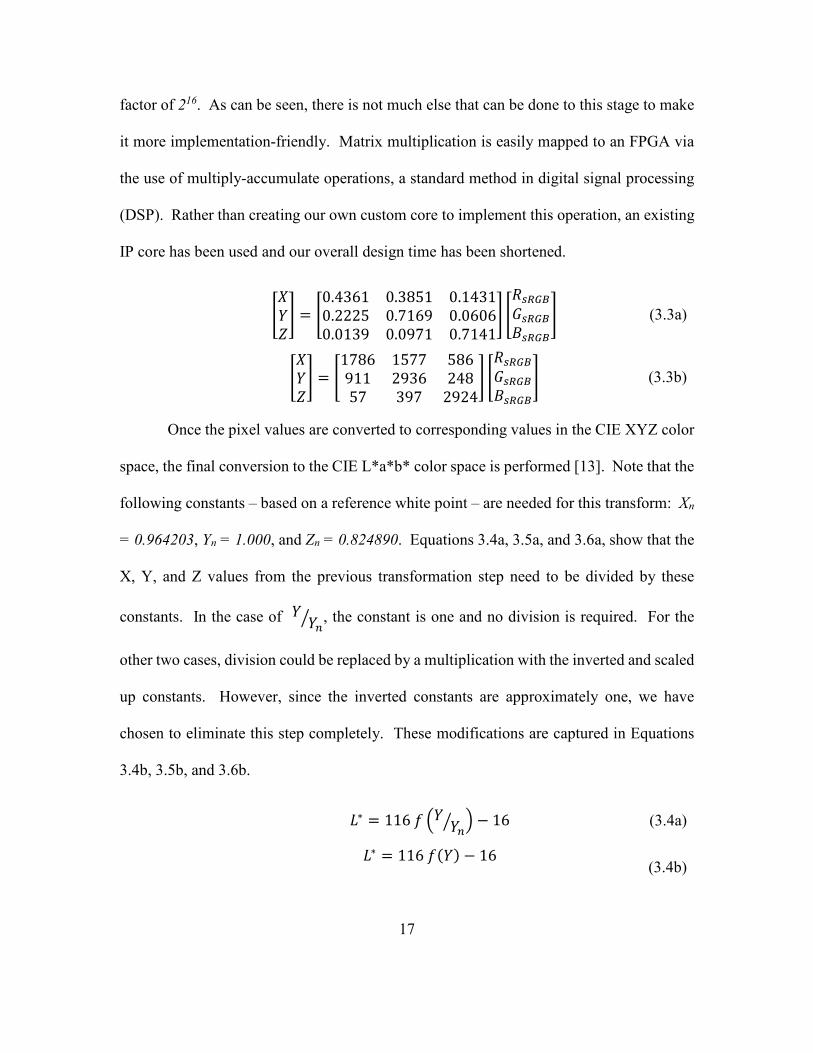
17

factor of 216. As can be seen, there is not much else that can be done to this stage to make

it more implementation-friendly. Matrix multiplication is easily mapped to an FPGA via

the use of multiply-accumulate operations, a standard method in digital signal processing

(DSP). Rather than creating our own custom core to implement this operation, an existing

IP core has been used and our overall design time has been shortened.

6789: = 60.4361 0.3851 0.14310.2225 0.7169 0.06060.0139 0.0971 0.7141: 6���������: (3.3a)

6789: = 61786 1577 586911 2936 24857 397 2924: 6���������: (3.3b)

Once the pixel values are converted to corresponding values in the CIE XYZ color

space, the final conversion to the CIE L*a*b* color space is performed [13]. Note that the

following constants – based on a reference white point – are needed for this transform: Xn

= 0.964203, Yn = 1.000, and Zn = 0.824890. Equations 3.4a, 3.5a, and 3.6a, show that the

X, Y, and Z values from the previous transformation step need to be divided by these

constants. In the case of 8 8<� , the constant is one and no division is required. For the

other two cases, division could be replaced by a multiplication with the inverted and scaled

up constants. However, since the inverted constants are approximately one, we have

chosen to eliminate this step completely. These modifications are captured in Equations

3.4b, 3.5b, and 3.6b.

=∗ = 116 � ,8 8<� . − 16 (3.4a)

=∗ = 116 ��8� − 16

(3.4b)

18

@∗ = 500 A� ,7 7<� . − � ,8 8<� .B (3.5a)

@∗ = 500 C��7� − ��8�D

(3.5b)

E∗ = 200 A� ,8 8<� . − � ,9 9<� .B (3.6a)

E∗ = 200 C��8� − ��9�D (3.6b)

Function f(x) is a piece-wise function [13] and is given in Equation 3.7a. Since the

input values to this step are scaled by a factor of 216, the constant value that the input values

are compared against must also be scaled by the same factor – which is a similar

modification to the one performed in Equations 3.2a. In the first case of Equation 3.7a, a

cube root operation is required. To create a custom core to perform this operation would

be time consuming and there are no pre-existing Xilinx IP cores for this operation. Using

a set of basic algebraic manipulations, the cube root operation can be replaced by the

product of multiple square root iterations, as shown in Equation 3.7b. To handle the second

case of Equation 3.7a the constant 7.787 can be rounded to 8.0, which effectively replaces

the multiplication with a three bit-shifts to the left. The addition of a constant value must

be scaled by 216 in order to match the scaling already applied to the input value. These

changes are shown in Equation 3.7b.

���� = F���G H� , )� > 0.0088567.787��� + 16 116� , )� ≤ 0.008856 (3.7a)

���� = I���G 2� ���G GJ� , )� > 580�� ≫ 3� + 9040, )� ≤ 580 (3.7b)

19

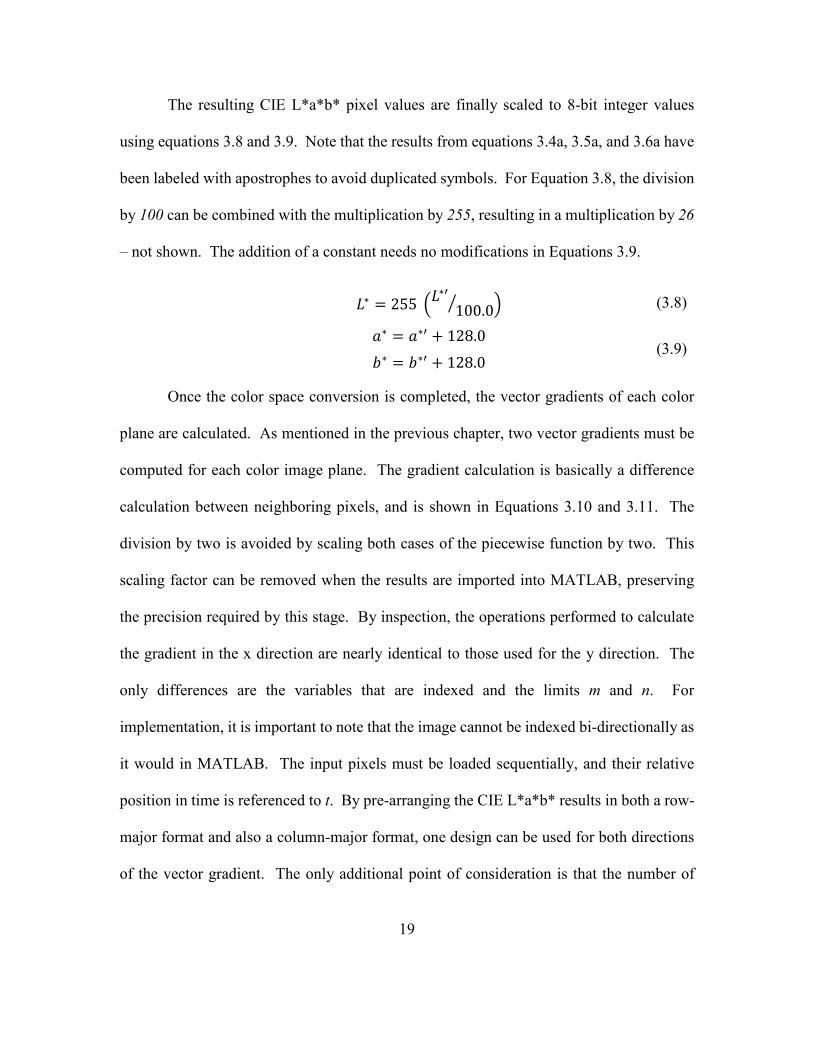
The resulting CIE L*a*b* pixel values are finally scaled to 8-bit integer values

using equations 3.8 and 3.9. Note that the results from equations 3.4a, 3.5a, and 3.6a have

been labeled with apostrophes to avoid duplicated symbols. For Equation 3.8, the division

by 100 can be combined with the multiplication by 255, resulting in a multiplication by 26

– not shown. The addition of a constant needs no modifications in Equations 3.9.

=∗ = 255 ,= ∗ 100.0� . (3.8)

@∗ = @∗ + 128.0 E∗ = E∗ + 128.0 (3.9)

Once the color space conversion is completed, the vector gradients of each color

plane are calculated. As mentioned in the previous chapter, two vector gradients must be

computed for each color image plane. The gradient calculation is basically a difference

calculation between neighboring pixels, and is shown in Equations 3.10 and 3.11. The

division by two is avoided by scaling both cases of the piecewise function by two. This

scaling factor can be removed when the results are imported into MATLAB, preserving

the precision required by this stage. By inspection, the operations performed to calculate

the gradient in the x direction are nearly identical to those used for the y direction. The

only differences are the variables that are indexed and the limits m and n. For

implementation, it is important to note that the image cannot be indexed bi-directionally as

it would in MATLAB. The input pixels must be loaded sequentially, and their relative

position in time is referenced to t. By pre-arranging the CIE L*a*b* results in both a row-

major format and also a column-major format, one design can be used for both directions

of the vector gradient. The only additional point of consideration is that the number of

20

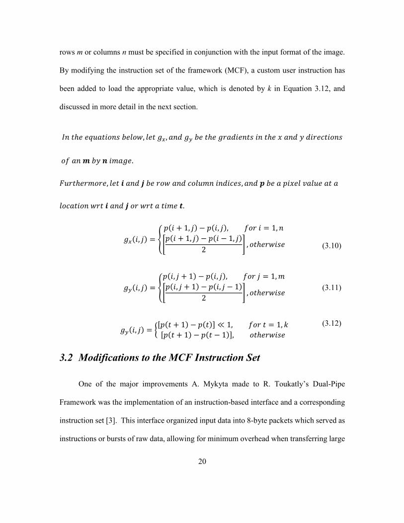
rows m or columns n must be specified in conjunction with the input format of the image.

By modifying the instruction set of the framework (MCF), a custom user instruction has

been added to load the appropriate value, which is denoted by k in Equation 3.12, and

discussed in more detail in the next section.

�K Lℎ& &NO@L)PK( E&'PQ, '&L �R, @K� �S E& Lℎ& �T@�)&KL( )K Lℎ& � @K� � �)T&UL)PK(

P� @K V E� W )X@�&. YOTLℎ&TXPT&, '&L Z @K� [ E& TPQ @K� UP'OXK )K�)U&(, @K� \ E& @ ])�&' ^@'O& @L @ 'PU@L)PK QTL Z @K� [ PT QTL @ L)X& _.

�R�), `� = a ]�) + 1, `� − ]�), `�, �PT ) = 1, Kb]�) + 1, `� − ]�) − 1, `�2 c , PLℎ&TQ)(&

(3.10)

�S�), `� = a]�), ` + 1� − ]�), `�, �PT ` = 1, Xb]�), ` + 1� − ]�), ` − 1�2 c , PLℎ&TQ)(& (3.11)

�S�), `� = dC]�L + 1� − ]�L�D ≪ 1, �PT L = 1, fC]�L + 1� − ]�L − 1�D, PLℎ&TQ)(& (3.12)

3.2 Modifications to the MCF Instruction Set

One of the major improvements A. Mykyta made to R. Toukatly’s Dual-Pipe

Framework was the implementation of an instruction-based interface and a corresponding

instruction set [3]. This interface organized input data into 8-byte packets which served as

instructions or bursts of raw data, allowing for minimum overhead when transferring large

21

amounts of data. The generic instruction word format, seen in Figure 3.1, was built to meet

requirements for PR and the HP CSC engine, while also allowing for custom user actions

to be added in the future.

Figure 3.1: A. Mykyta’s Generic Instruction Word Format, Reproduced from [3].

Leveraging the flexibility of the instruction word format, a new instruction word

was created for the vector gradient modules. The custom user instruction Ld Gradient

Counter is automatically sent after the Flush MCF and Channel Sync commands when the

vector gradient processing module is specified in the MCF job script. This command loads

a register in the custom user circuit with the height or width, in pixels, of the image being

processed. This value was denoted by k in the previous section and is required to trigger

special cases of subtraction when the edges of the image are being processed. By

modifying the instruction set to add this capability to the user circuit, one vector gradient

module was able to be used for both the x direction and y direction gradients.

The various operations built into the instruction set were separated into non-

processing commands and CSC commands. The instruction added during the course of

this work has been classified as a custom command, as it does not pertain to HP’s CSC

engine, a PR operation, or other routine channel control operations. A summary of all

22

current MCF instructions is presented in Table 3.1, with the custom command appended to

the instruction words from the work of A. Mykyta et al..

Bit Position 63 62 61 60 ... 56

User

Instruction

Burst

Start

PR

Instruction Operation Resulting

Opcode

Non-Processing Commands:

No Operation 0 0 0 0x0 0x00

Start PR Burst Data 0 1 1 0x1 0x61

Flush MCF 0 0 0 0x2 0x02

Channel Sync 0 0 0 0x8 0x08

CSC Commands:

Reg-Bus Write 1 0 0 0x1 0x81

Start Pixel Burst 1 1 0 0x2 0xC2

Custom Commands:

Ld Gradient Counter 1 1 0 0x5 0x85

Table 3.1: Supported Instruction Word Opcodes, modified from [3].

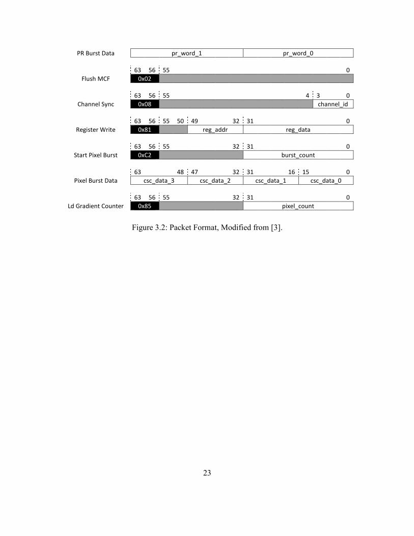
The corresponding packet format for the Ld Gradient Counter custom instruction

word is shown in Figure 3.2. The packet format is very similar to a Start PR Data Burst

instruction or a Start Pixel Burst Instruction. The similar format allowed for a very quick

and effortless implementation of the new instruction. The modified packet format diagram

is included for completeness and shows how all 8-bytes are used for each instruction. Note

that gray areas in the figure represent bits that are unused.

63 56 55 0

No Operation 0x00

63 56 55 32 31 0

Start PR Data Burst 0x61 burst_count

63 32 31 0

23

PR Burst Data pr_word_1 pr_word_0

63 56 55 0

Flush MCF 0x02

63 56 55 4 3 0

Channel Sync 0x08 channel_id

63 56 55 50 49 32 31 0

Register Write 0x81 reg_addr reg_data

63 56 55 32 31 0

Start Pixel Burst 0xC2 burst_count

63 48 47 32 31 16 15 0

Pixel Burst Data csc_data_3 csc_data_2 csc_data_1 csc_data_0

63 56 55 32 31 0

Ld Gradient Counter 0x85 pixel_count

Figure 3.2: Packet Format, Modified from [3].

24

Chapter 4: Design for Implementation

In the previous chapter, the first steps of the GSEG algorithm were modified to

achieve an efficient implementation in an FPGA. The design flow used during this process

was documented and a set of design guidelines were generated from observations. The

design flow and guidelines have been paired to develop a general methodology for tailoring

algorithms for implementation. In this chapter, the Design for Implementation (DFI)

methodology is presented in detail.

4.1 Design for Implementation Flow

In order to justify or validate the algorithm modifications presented in the previous

chapter, a metric is needed to observe and evaluate changes in the resulting image. With a

metric selected, a threshold is chosen based on what is considered acceptable image

degradation for the given application. The selection of image quality metrics and the

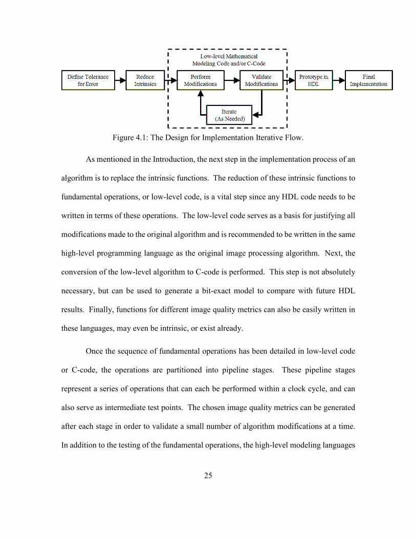
definition of tolerable error serve as the initial step in the DFI flow, which is illustrated in

Figure 4.1. The image quality metrics used to evaluate the GSEG algorithm modifications

are discussed in more detail in the next chapter.

25

Figure 4.1: The Design for Implementation Iterative Flow.

As mentioned in the Introduction, the next step in the implementation process of an

algorithm is to replace the intrinsic functions. The reduction of these intrinsic functions to

fundamental operations, or low-level code, is a vital step since any HDL code needs to be

written in terms of these operations. The low-level code serves as a basis for justifying all

modifications made to the original algorithm and is recommended to be written in the same

high-level programming language as the original image processing algorithm. Next, the

conversion of the low-level algorithm to C-code is performed. This step is not absolutely

necessary, but can be used to generate a bit-exact model to compare with future HDL

results. Finally, functions for different image quality metrics can also be easily written in

these languages, may even be intrinsic, or exist already.

Once the sequence of fundamental operations has been detailed in low-level code

or C-code, the operations are partitioned into pipeline stages. These pipeline stages

represent a series of operations that can each be performed within a clock cycle, and can

also serve as intermediate test points. The chosen image quality metrics can be generated

after each stage in order to validate a small number of algorithm modifications at a time.

In addition to the testing of the fundamental operations, the high-level modeling languages

26

lend well to the generation of test vectors that are necessary to validate any C and HDL

code. After laying out the pipeline stages, the design is prototyped using an HDL such as

Verilog or VHDL. Again, the results generated from the HDL, whether from a test bench

or emulation, can be verified using the same high-level programming language as before.

4.2 Design for Implementation Guidelines

As presented in Chapter 3 and validated by the results in Chapter 6, during the

design for implementation process of the GSEG algorithm, it was discovered that a number

of changes made to the original algorithm resulted in a more efficient implementation.

These were compiled into a set of guidelines that, when coupled with the design flow, form

the DFI methodology.

At the present time, the DFI guidelines are:

• Selecting an appropriate image quality metric and defining a tolerable amount of

degradation.

The tolerance for error in the overall result of the algorithm is a valuable parameter

as it will be used to validate all modifications made to the original algorithm. Once it has

been defined, it serves as the basis for evaluating the results of the remaining guidelines.

This prevents striving for functional correctness at a higher precision than is required by

an application, a practice which should be avoided as much as possible.

• Using minimal operand representation ranges.

27

In high-level models of algorithms, standard operand sizes are often used. This is

perfectly acceptable for achieving functional correctness, but implementing a 64-bit

floating-point number is very costly, especially if only eight to sixteen bits are required.

Selecting efficient representation ranges for operands is an easy way to reduce resource

utilization and congestion during implementation.

• Using scale factors to represent fractional numbers as fixed-point integers.

o Subsequently, using integer arithmetic units whenever possible.

The use of floating-point numbers also requires the use of floating-point arithmetic

units. This can be avoided by using large constant multipliers as scale factors. By scaling

fractional numbers up to integers, any required amount of precision can be preserved. This

allows for the use of standard integer arithmetic units, which require fewer resources than

floating-point units.

• Rounding constant multipliers/divisors to powers of two.

When the second operand of a multiplication or division is a constant that can be

reasonably rounded to a power of two, the operation can be effectively eliminated. The

determination of “reasonably” is left to the expertise of the algorithm developer and his

definition of tolerable degradation. If this method of rounding is not acceptable, round

constants to the nearest integer and try to apply the next guideline.

• Avoiding division at all costs.

As was mentioned in the previous chapter, division can be performed in a variety

of ways, any of which are costly. In the cases where the divisor is a constant, division can

28

always be replaced by multiplication. The constant can be inverted, and if a fractional

portion remains, another scale factor can be applied to facilitate integer multiplication. For

cases where the divisor is not a constant and no simplifications exist, then action should be

taken to use a division algorithm that is most efficient for the application. This may require

weighing a tradeoff between execution time and resource utilization.

• Using pre-existing IP cores whenever possible.

Chances are that most of the operations required by an algorithm have already been

implemented as IP cores or even custom cores. Having a working knowledge of the cores

available to the hardware designer should influence the operations chosen by the algorithm

developer when the DFI methodology is applied.

• Accepting an approximate operation.

For cases where no pre-existing cores are applicable, an approximate operation may

be required (e.g., approximation of the cube root presented in Chapter 3). Consider suitable

replacement operations and evaluate their effects based on metrics or subjective evaluation

of the resulting image. A custom core or adaptation of an existing core may ultimately be

necessary if the approximation is not tolerable.

• Applying the DFI process iteratively.

With a tolerable level of image degradation already defined, multiple iterations of

the DFI process can be performed until a maximally efficient design is achieved. As G.

Karakonstantis et al. noted in [8], different portions of a given algorithm can contribute

different amounts to overall image quality. Numerous combinations of different

29

modifications could result in reaching the threshold of image quality; however, some may

be more efficient than others in terms of standard implementation parameters. That is, the

tolerable level of image degradation may be reached solely by maximally reducing the

representation range of the operands and data buses. On the other hand, the same level of

image degradation could be achieved by balancing a reduction in representation range and

also an approximation of an operation. These tradeoffs should be considered by the

designer in order to achieve a truly efficient algorithm implementation for their given

application.

4.3 General Applicability of the Proposed Methodology

The major benefit of the DFI methodology is that it is ultimately flexible in nature.

As algorithm developers likely have their own design process based upon experience, it

was imperative to propose a design methodology that could be used as an addendum to

their current processes. This allows the methodology to be applied to algorithms that have

already been designed, as well as algorithms that are currently in development. Once a

developer has been introduced to the concepts of designing for implementation, it is likely

that many of the guidelines will be taken into account as supplemental procedures during

their own design process.

An additional benefit of the methodology is that it is inherently an iterative process,

meaning that multiple iterations of its application to an algorithm will eventually converge

to an optimal solution. This concept, however, also presents a potential pitfall. As has

been mentioned previously in this work, different aspects of an image processing algorithm

30

can contribute differently to overall image quality [8], but also impact other design

parameters. Elaborating further, an inexperienced developer could spend the majority of

their time attempting to optimize a portion of the algorithm that won’t result in a noticeable

reduction in execution time, logic utilization, or power consumption. For this reason, a

method of analyzing the savings attributed to the different guidelines presented in the

previous section would be useful. This could be done with a type of cost-table solution for

different transforms and guidelines, but such an addition would be done as future research

and would require the application of this methodology on a variety of image processing

algorithms.

The flexibility of this methodology provides potential for it to be applied in other

areas of digital implementation. Although the proposed methodology was designed with

image processing algorithms in mind, a majority of the concepts presented in the guidelines

are applicable to any type of digital processing algorithm that needs to be implemented in

hardware, such as any DSP algorithms. Before it could be applied to other fields, however,

a tolerance for error would need to be defined specific to the application desired. That is,

a parameter that is analogous to image quality in this work would need to be identified.

31

Chapter 5: Implementation of the Test

Vehicle

In the previous two chapters, an example of designing an algorithm for

implementation and a design for implementation methodology were shown. The DFI

methodology can transform high-level MATLAB code into synthesizable HDL code,

according to the design flow presented in Chapter 4. In this chapter, the overall process of

implementing the various modules from MATLAB code is described in detail. More

specifically, the conversions between different programming languages and programming

levels are discussed.

5.1 Conversions between Programming Languages

As was introduced earlier in this work, algorithms are often developed using high-

level modeling languages such as MALAB or MAPLE. While these languages are well

suited for fine-tuning parameters and quickly testing an algorithm, they do not discretely

call out hardware resources. For this reason, the first step leading to synthesizable HDL is

to dissect the algorithm within the high-level modeling language. By dissecting the

algorithm, the fundamental operations can be identified and used to replace any intrinsic

functions that have been called. This is a crucial step for targeting hardware and for even

writing C-code, as MATLAB functions (for an example) do not always directly translate

to functions in C.

32

Converting the high-level model of the algorithm into a low-level model, using the

same programming language, is a relatively quick way to verify that the fundamental

operations and representation ranges identified were correct. Once the low-level model is

written in terms basic operations or functions for which the details are known, a C-code

version can be written. In principal, a C-code model could be written directly from the

high-level model of the algorithm, however it would not be as easy to verify the operations.

Regardless of whether or not a low-level model is created as an intermediate step, the

conversion from a high-level modeling language to C-code presents a number of

difficulties. Using MATLAB as an example language for a starting point, the

complications experienced from a conversion to C-code are presented here.

The first problem encountered was the ability for an intrinsic function to have other

intrinsic functions called as the input. The nesting of multiple functions as the input of a

function presents two kinds of challenges. One challenge is that this piece of code is much

longer and more complex than it seems at first glance. The dissection of one of these lines

of code, depending upon the level of nesting involved, can take considerably longer than

expected resulting in poor estimations of overall development time requirements. A

second challenge arising from this coding style is that the code becomes much more

difficult to navigate and step through in the debugger. One must take careful consideration

to track which function they are actually stepping through. The representation ranges and

variable types being used may change throughout these nested functions and must also be

taken into consideration.

33

This leads directly into the next difficulty experienced with such a conversion

between languages. Most MATLAB functions have multiple options for a given operation

based on the input type, since the input types aren’t known until execution time.

Additionally, input parameters can be added to certain intrinsic functions or defaults will

be used if none are specified. These make a conversion to C-code more difficult, as some

functions may change based upon input type. One example of this is the basic histogram

function. Without going into great detail, one can see that the creation of an 8-bit histogram

is slightly different than that of a 16-bit histogram. Again, this would likely not be

considered when writing the high-level model in MATLAB, however, when writing a C-

code model these details need to be known.

Other complications are the special operators that are intrinsic within MATLAB.

Operators such as [ ], ‘, and (:) are specifically matrix declarations and matrix math

operations. The [ ] operator is used to declare arrays and matrices in-line, and the (:)

operator is used to denote an entire row of an array. The special operator ‘ denotes a matrix

transposition, which would require a number of for-loops to implement in C-code.

Additionally, the matrix mathematic versions of multiplication and division require

multiple for-loops to implement. There are number of other special operators that do not

map directly to a C function, adding complexity to the conversion between languages.

As mentioned earlier in this section, the input types are not known to the function

until execution. To add to this complication, the sizes are not known either. Take the

following lines of MATLAB code as an example:

%%Sample MATLAB Code:

34

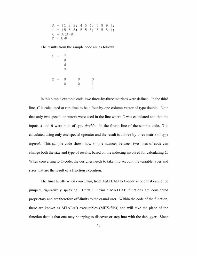
A = [1 2 3; 4 5 6; 7 8 9;]; B = [5 5 5; 5 5 5; 5 5 5;]; C = A(A>B) D = A>B

The results from the sample code are as follows: C = 7

8 6 9

D = 0 0 0 0 0 1 1 1 1

In this simple example code, two three-by-three matrices were defined. In the third

line, C is calculated at run-time to be a four-by-one column vector of type double. Note

that only two special operators were used in the line where C was calculated and that the

inputs A and B were both of type double. In the fourth line of the sample code, D is

calculated using only one special operator and the result is a three-by-three matrix of type

logical. This sample code shows how simple nuances between two lines of code can

change both the size and type of results, based on the indexing involved for calculating C.

When converting to C-code, the designer needs to take into account the variable types and

sizes that are the result of a function execution.

The final hurdle when converting from MATLAB to C-code is one that cannot be

jumped, figuratively speaking. Certain intrinsic MATLAB functions are considered

proprietary and are therefore off-limits to the casual user. Within the code of the function,

these are known as MTALAB executables (MEX-files) and will take the place of the

function details that one may be trying to discover or step-into with the debugger. Since

35

these functions don’t give the user any insight as to what calculations are taking place, the

only way around them is to research similar functions. Once a number of possible functions

are found from literature, they can be modeled in MATLAB and the results can be

compared. In some cases, the algorithms found during this research may have results that

match MATLAB’s results exactly. Other times, an approximation can be found and the

results have to be deemed acceptable for the application in order to move forward.

In fact, for almost all algorithm steps presented in Chapter 3, the results were

reproduced exactly with the low-level model (without modifications). For the conversion

from sRGB to linear sRGB, an approximate function is being used. The color space

conversion function implemented by MATLAB uses curve-fitting procedures that were

deemed inefficient for the hardware implementation in this work. A review of literature

regarding color space conversions found an alternative piecewise function for the

operation, which was shown in Chapter 3. The results produced by the low-level model of

the alternative function were deemed to be acceptable for the application when compared

to the intrinsic MATLAB function’s results.

5.2 Image Quality Metrics and Validation

Since the original GSEG algorithm is written using MATLAB, it is natural to use

MATLAB to create the low-level model of the GSEG algorithm and therefore to validate

its results. The first step in applying the DFI methodology, as was presented in Chapter 4,

is to identify a metric, or a number of metrics, to be used for evaluating algorithm

modifications. In order to validate the algorithm modifications made in Chapter 3, Section

36

1, test images and image quality metrics are selected. The same images database used for

evaluating the GSEG algorithm [15] is selected to evaluate the DFI methodology. By using

this database, any degradation or effects on the overall segmentation maps can be assessed

by comparison with original GSEG results.

Next, the image quality metrics are selected. Those chosen include: the 2-

dimensional correlation coefficient [16] (CORR2), the peak signal-to-noise ratio [17]

(PSNR), and the structural similarity index [18] (SSIM). Each of the metrics selected can

only compare two two-dimensional image planes, which are represented by variables f and

g in the equations presented in this section. Thus, if an RGB image is being compared to

a known good image, three CORR2 results would be calculated, one for each red, green,

and blue plane.

The 2D correlation coefficient is selected for its ease of use, as it is an intrinsic

MATLAB function. Another advantage is that it produces a single result, between zero

and one, as opposed to a matrix of results for the image plane being validated. The CORR2

function shows the linear dependence, or lack thereof, between the two planes by way of

Equation 5.1, and the result is denoted by r.

T��, �� = ∑ ∑ h�i,< − �j̅h�i,< − �̅j<i

5,∑ ∑ h�i,< − �j̅1<i . ,∑ ∑ h�i,< − �̅j1<i . (5.1)

The next two image quality metrics are chosen based on a literature review of

industry standard methods for comparing the likeness of two images, the first of which is

the Peak Signal to Noise Ratio. Calculating the PSNR is a two part process, beginning

37

with the Mean Squared Error (MSE) in Equation 5.2a. The PSNR is then calculated in

decibels using the MSE and the total number of bits used to represent a pixel’s value,

denoted as b in Equation 5.2b.

klm��, �� = ∑ ∑ h�i,< − �i,<j1<i XK (5.2a)

nlo� = 'P�Gp �2� − 1�1klm �� (5.2b)

The structural similarity index (SSIM) is the final metric selected to evaluate the

modifications made to the GSEG algorithm. The SSIM method is chosen in addition to

the PSNR method, since it has been shown that specific cases of image degradation are not

reflected by the PSNR [18]. Namely, when the MSE is equal to zero the PSNR does not

reflect the difference in image quality. Although the SSIM equations are not presented

here in detail, they can be found in their original publication [18]. The authors also

provided a MATLAB function for calculating the SSIM index, which is used in this work

[19].

Since one of the image quality metrics is an intrinsic MATLAB function and

another is provided in MATLAB from [19], it is again natural to validate the modifications

using MATLAB. To reduce the overhead of testing for future images, a number of

MATLAB scripts were written to automate the process. The loading of known good

images, reorganization of pixels, scaling, and displaying of results are just some of the

functions handled by the scripts. These scripts are used to evaluate the images at every

step throughout the DFI design flow such as low-level MATLAB code results, C-code

results from the host PC, Verilog test bench results, and MCF emulation results. The

38

repetitive use of the scripts ensured that there were no discrepancies or user errors between

tests.

5.3 Test Setup

This section describes the software and hardware used throughout this work. The

high-level programming language used was MATLAB version 7.11.0, release name

R2010b. All low-level code was written in MATLAB, as well as functions for generating

image quality metrics, when not provided. For generating HDL, Xilinx ISE Design Suite

14.5 was used. Plan Ahead version 14.5, with a Partial Reconfiguration license, was used

for generating bit-streams while iMPACT was used for programming. The FPGA targeted

was a Virtex-6, as part of the Xilinx ML605 XC6VLX240T-1FFG1156 evaluation board.

All programming of the FPGA was performed via JTAG over USB.

All software tools were used on a Windows 7 PC (x86, SP1) with an Intel Core 2 Duo

CPU (2.4 GHz) and 3 GB of RAM. For C-code generation and testing, a separate PC was

used running Linux Fedora 10 (2.6.27.5 Kernel version) which also had an Intel Core 2

Duo (2.4 GHz) CPU. This PC is commonly referred to as the host PC throughout this thesis

and had 2 GB of RAM. The PCIe slot was populated with the ML605 FPGA card. Code

was written and modified using gedit, and compiled with the GNU C compiler and GNU

make. All of this information is presented in list form as Appendix A, located after the

References.

39

Chapter 6: Results and Discussions

In this chapter, the results from emulating the first steps of the GSEG algorithm are

presented and discussed. First, the algorithm modifications made in Chapter 3 are validated

using the image quality metrics presented in Chapter 5. Next, some emulation result

images are shown in comparison to the known good images. Finally, design parameters of

interest are presented. These include logic utilization, power consumption, and execution

time for each processing module.

6.1 Validation of Algorithm Modifications

The following results represent different image quality metrics for each stage of the

algorithm. Two images were selected from the database, one of which was of two deer

(321 pixels by 481 pixels) and another of which was two officers in front of a clock tower

(481 pixels by 321 pixels). The test points compare original algorithm results generated in

MATLAB with the modified algorithm results generated from implementation within the

FPGA. In the presentation of the vector gradient results, for a given image plane gradients

corresponding to the x direction are denoted by � �� � . Likewise, gradients corresponding

to the y direction are denoted by � �� � . It is important to note that these results represent

each stage tested independently from one another, meaning that results from each stage of

the original, unmodified algorithm are used as test inputs. This ensures that any

degradation from a previous stage does not affect the outcome of the stage being evaluated.

In this paper, the modifications of each stage are evaluated individually. Future work will

40

evaluate the degradation from all stages sequentially and the overall effects of this

processing on the segmentation map.

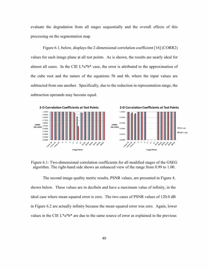
Figure 6.1, below, displays the 2-dimensional correlation coefficient [16] (CORR2)

values for each image plane at all test points. As is shown, the results are nearly ideal for

almost all cases. In the CIE L*a*b* case, the error is attributed to the approximation of

the cube root and the nature of the equations 5b and 6b, where the input values are

subtracted from one another. Specifically, due to the reduction in representation range, the

subtraction operands may become equal.

Figure 6.1: Two-dimensional correlation coefficients for all modified stages of the GSEG

algorithm. The right-hand side shows an enhanced view of the range from 0.99 to 1.00.

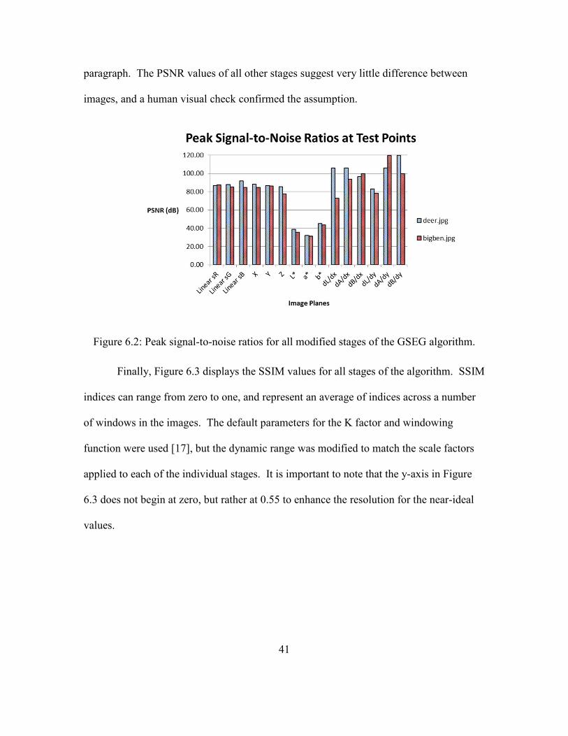
The second image quality metric results, PSNR values, are presented in Figure 4,

shown below. These values are in decibels and have a maximum value of infinity, in the

ideal case where mean squared error is zero. The two cases of PSNR values of 120.0 dB

in Figure 6.2 are actually infinity because the mean squared error was zero. Again, lower

values in the CIE L*a*b* are due to the same source of error as explained in the previous

41

paragraph. The PSNR values of all other stages suggest very little difference between

images, and a human visual check confirmed the assumption.

Figure 6.2: Peak signal-to-noise ratios for all modified stages of the GSEG algorithm.

Finally, Figure 6.3 displays the SSIM values for all stages of the algorithm. SSIM

indices can range from zero to one, and represent an average of indices across a number

of windows in the images. The default parameters for the K factor and windowing

function were used [17], but the dynamic range was modified to match the scale factors

applied to each of the individual stages. It is important to note that the y-axis in Figure

6.3 does not begin at zero, but rather at 0.55 to enhance the resolution for the near-ideal

values.

42

Figure 6.3: Structural similarity indices for all modified stages of the GSEG algorithm.

The results presented in this paper suggest that modifications can be made to an

algorithm design with minimal effects on image quality. All image planes are subject a

human visual check in addition to the image quality metrics. This ensures that there are

no cases of image degradation that were missed by the metrics.

6.2 Cases of Significant Degradation

The image quality data presented in the previous section suggests that the first two

GSEG modules implemented produced ideal results. Since there was negligible image

degradation, the linear sRGB results and CIE XYZ results are not discussed in this section.

The CIE XYZ to CIE L*a*b* conversion, which featured the approximation of the cube

root via successive iterations of a square root and a multiplication, was expected to be the

most compromising implementation in terms of image quality. The results from the

43

previous section confirmed this hypothesis. Degradation was visible for this module and

two separate cases are shown in the next paragraph.

The first case shown is for the picture of two deer, referred to as deer.jpg in the

previous three figures. Two images are shown for comparison in Figure 6.4 and Figure 6.5

of the known good image and the MCF emulation result, respectively. Although they are

shown in black and white here, color versions are provided in Appendix B, at the end of

this thesis. The degradation is more easily seen as “fuzziness” in a blown up version of

the image on the right, however, at this size one would struggle to find any major

discrepancies.

Figure 6.4 (LEFT): The GSEG result in the CIE L*a*b* color space.

Figure 6.5 (RIGHT): The MCF result in the CIE L*a*b* color space.

The second case shown is for the picture of two officers standing in front of the Big

Ben clock tower, referred to as bigben.jpg in the image quality bar graphs. Two images are

shown for comparison in Figure 6.6 and Figure 6.7 of the known good image and the MCF

emulation result, respectively. Again, black and white versions of the images are shown,

but the color versions can be found in Appendix B. In this case, the degradation is much

44

more visible in the form of striations in the sky of the picture. This is a good example of

the content of the image may react differently to the modifications made in the algorithm.

On one hand, the image of the deer would appear to be almost identical, but on the other

hand the image of the two officers might be considered unacceptable. Such is not the case

for our GSEG algorithm, as features such as texture modeling can be tuned to avoid

segmenting the striations. These results confirm that different applications can tolerate

different amounts of degradation.

Figure 6.6 (LEFT): The GSEG result in the CIE L*a*b* color space.

Figure 6.7 (RIGHT): The MCF result in the CIE L*a*b* color space.

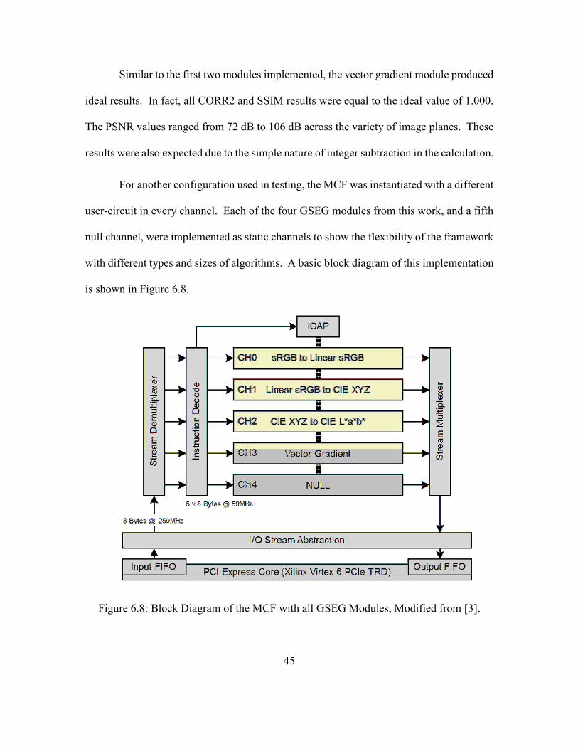
45

Similar to the first two modules implemented, the vector gradient module produced

ideal results. In fact, all CORR2 and SSIM results were equal to the ideal value of 1.000.

The PSNR values ranged from 72 dB to 106 dB across the variety of image planes. These

results were also expected due to the simple nature of integer subtraction in the calculation.

For another configuration used in testing, the MCF was instantiated with a different

user-circuit in every channel. Each of the four GSEG modules from this work, and a fifth

null channel, were implemented as static channels to show the flexibility of the framework

with different types and sizes of algorithms. A basic block diagram of this implementation

is shown in Figure 6.8.

Figure 6.8: Block Diagram of the MCF with all GSEG Modules, Modified from [3].

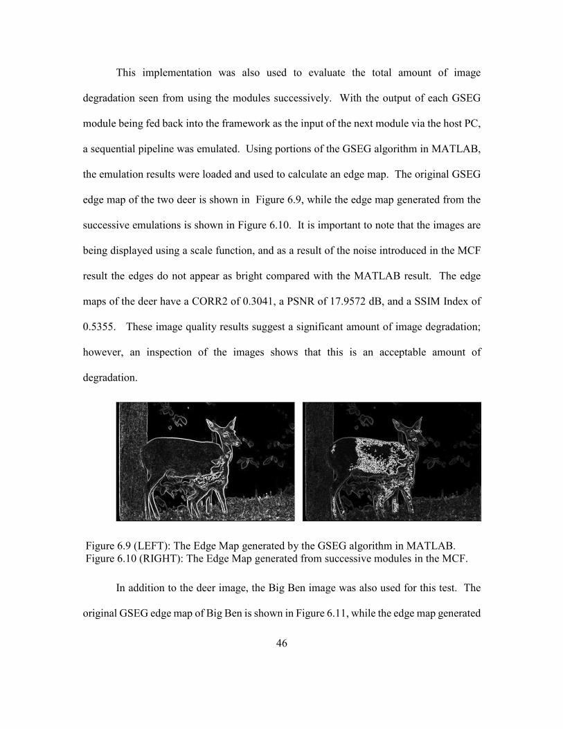
46

This implementation was also used to evaluate the total amount of image

degradation seen from using the modules successively. With the output of each GSEG

module being fed back into the framework as the input of the next module via the host PC,

a sequential pipeline was emulated. Using portions of the GSEG algorithm in MATLAB,

the emulation results were loaded and used to calculate an edge map. The original GSEG

edge map of the two deer is shown in Figure 6.9, while the edge map generated from the

successive emulations is shown in Figure 6.10. It is important to note that the images are

being displayed using a scale function, and as a result of the noise introduced in the MCF

result the edges do not appear as bright compared with the MATLAB result. The edge

maps of the deer have a CORR2 of 0.3041, a PSNR of 17.9572 dB, and a SSIM Index of

0.5355. These image quality results suggest a significant amount of image degradation;

however, an inspection of the images shows that this is an acceptable amount of

degradation.

Figure 6.9 (LEFT): The Edge Map generated by the GSEG algorithm in MATLAB.

Figure 6.10 (RIGHT): The Edge Map generated from successive modules in the MCF.

In addition to the deer image, the Big Ben image was also used for this test. The

original GSEG edge map of Big Ben is shown in Figure 6.11, while the edge map generated

47

from the successive emulations is shown in Figure 6.12. Again, scaling is applied to

display the images. The two edge maps of Big Ben have a CORR2 of 0.5833, a PSNR of

18.5982 dB, and an SSIM Index of 0.4070. Similar to the case of the deer image, the image

quality results suggest significant image degradation. A visual inspection shows that this

is an acceptable edge map, with the majority of the degradation seen in the windows of the

clock tower and as striations in the sky.

Figure 6.11 (LEFT): The Edge Map generated by the GSEG algorithm in MATLAB.

Figure 6.12 (RIGHT): The Edge Map generated from successive modules in the MCF.

6.3 Logic Utilization, Power Consumption, and Execution Time

Before presenting the logic utilization and power consumption results, it is important

to note the final configuration of the framework used for testing purposes. Seen in Figure

6.13, the MCF is instantiated with all four GSEG modules and the 3D HP CSC engine.

This configuration provides results for analyzing how resource utilization scales as

different modules are instantiated within the framework. It also shows that the

48

implementation of the GSEG modules in the other channels do not hinder the operation of

the HP CSC engine in the final channel, which continued produced known good results

under testing.

Figure 6.13: Block Diagram of the MCF with five channels utilized, Modified from [3].

Four modules were implemented in the Virtex-6 FPGA as a result of partitioning the

beginning portions of the GSEG algorithm. The logic utilization numbers for each of the

individual modules is presented in Table 6.1. This table also includes the logic utilization

numbers for the multichannel framework and PCIe interface. As one can see by inspection,

the modules were not large. Although a verbatim implementation of the GSEG algorithm

does not exist for comparison, savings can be inferred based upon the modifications

presented in Chapter 3. By reducing the representation ranges to the absolute minimum

49

for each module, fewer resources are used for routing and therefore the problem of

congestion is alleviated. Other modifications removed entire steps completely or

substituted IP cores to efficiently use DSP48 slices instead of Look-Up-Tables and Flip-

Flops, surely reducing logic utilization.

Slices FFs LUTs BRAM DSP48 BUFG BUFR MMCM

MCF 2,546 1,857 2,447 0 0 0 0 0

7% 1% 2% 0% 0% 0% 0% 0%

PCIe 12,094 26,721 20,568 75 0 11 2 2

32% 9% 14% 18% 0% 34% 6% 17%

GSEG Modules:

sRGB to Lin sRGB 91 137 243 0 9 2 0 0

0.24% 0.05% 0.16% 0% 1% 6% 0% 0%

Lin sRGB to XYZ 51 158 79 0 3 2 0 0

0.14% 0.05% 0.05% 0% 0% 6% 0% 0%

XYZ to L*a*b* 652 679 1973 0 2 1 0 0

1.7% 0.23% 1.3% 0% 0% 3% 0% 0%

Vector Gradient 116 201 234 0 0 2 0 0

0.31% 0.07% 0.16% 0% 0% 6% 0% 0%

Available in xc6vlx240t:

37,680 301,440 150,720 416 768 32 36 12

Table 6.1: FPGA Resource Utilization1, MCF & PCIe taken with permission from [3].

The individual module logic utilization numbers presented in Table 6.1 can be used

to predict the utilization numbers for implementing all four GSEG modules within the

framework. To predict utilization, all resource types except the BUFG (global buffer) can

be summed. The global clock buffers are associated with the interface to the PC, thus to

predict the BUFG usage for the configuration with four channels only the PCIe is

1 The utilization reported for each GSEG module does not include the MCF or PCIe logic.

50

considered. The logic utilization numbers for the two configurations previously mentioned

are presented in Table 6.2.

The first row of data corresponds to the prediction of resource usage suggested by

summing the individual module usage statistics. These numbers can be compared directly

to the second row, which is reported logic utilization for the corresponding implementation.

In only case did the logic usage actually decrease, which is likely due to the variations seen

between place and route operations. In the third and final row, the full five-channel

implementation utilization numbers are reported. As expected, the inclusion of the HP

CSC engine has caused an increase in most types of resources. The buffers (BUFG and

BUFR) and mixed mode clock managers (MMCM) were not expected to increase, as they

are associated with the PCIe interface only.

Slices FFs LUTs BRAM DSP48 BUFG BUFR MMCM

MCF 4-Channels

Suggested Utilization

15,550 29,753 25,544 75 14 11 2 2

41% 10% 17% 18% 2% 34% 6% 17%

MCF 4-Channels

(GSEG & Null)

13,135 30,430 28,190 75 14 11 2 2

35% 10% 19% 18% 2% 34% 6% 17%

MCF 5-Channels

(GSEG & CSC)

16,240 34,278 36,783 135 30 11 2 2

43% 11% 24% 32% 4% 34% 6% 17%

Available in xc6vlx240t:

37,680 301,440 150,720 416 768 32 36 12

Table 6.2: Logic Utilization for MCF Configurations with multiple active channels.

Once the modules were implemented within the framework, the XPower Analyzer

can be used to generate post-implementation power consumption estimations of each

design. As A. Mykyta et al. noted, the tool uses Xilinx’s own heuristics and activity factors

to calculate these estimates [3], which are shown in Table 6.3. It is important to note that

51

these power consumption numbers do not represent each module alone, but one instance

of the module along with the MCF and PCIe supporting hardware. The final two rows of

data correspond to the configurations with multiple active channels. All power

consumption statistics are estimated based on each channel operating at a frequency of 50

MHz and the PCIe interface operating at a frequency of 250 MHz.

A. Mykyta’s work showed that the MCF and PCIe logic contributed 2599 mW

toward dynamic power consumption [3]. Based on the numbers shown in Table 6.3, the

GSEG modules themselves consume an insignificant amount of power. This was

suggested by the low logic utilization parameters presented in Table 6.1. An interesting

result is that the power consumption estimate decreased for the implementation with four

GSEG modules when compared with each individual GSEG implementation. This is due

to the variations within the implementation process and the estimates based on

implementation results, which vary between runs.

Configuration mW

sRGB to Lin sRGB

Dynamic Power 2646

Quiescent Power 6388

Total 9034

Lin sRGB to XYZ

Dynamic Power 2648

Quiescent Power 6388

Total 9036

XYZ to L*a*b*

Dynamic Power 2649

Quiescent Power 6388

Total 9037

Vector Gradient

Dynamic Power 2651

Quiescent Power 6388

Total 9039

52

MCF 4-Channels (GSEG & Null)

Dynamic Power 2622

Quiescent Power 6387

Total 9009

MCF 5-Channels (GSEG & CSC)

Dynamic Power 2643

Quiescent Power 6388

Total 9031

Table 6.3: Power Consumption Estimates2.

Finally, the execution time for each module can be inferred due to the deterministic

nature of the image processing pipelines. Based on the clock frequency controlling the

advancement of data throughout the pipeline, the number of stages in each pipeline, the

number of bytes of data being processed, and the number of stages in input/output

abstraction layer developed in [3], the execution time for each module can be calculated.

These execution times are presented in Table 6.4, along with the original MATLAB

algorithm execution times. The first module has a latency of five 50 MHz clock cycles.

The Linear sRGB to CIE XYZ stage has a sub-pipeline operating at a clock frequency of

250 MHz, allowing the stage to have a latency of one 50 MHz clock cycle. In the case of

the CIE XYZ to CIE L*a*b* conversion, the pipeline has a latency of twelve 50 MHz clock

cycles, causing the execution time to be longer due the extra cycles required to fill and

empty the pipeline. The vector gradient module, on the other hand, has a latency of three

50 MHz clock cycles.

GSEG Module Execution Time (ms)

2 For the results shown in Table 6.3, each module has been instantiated as a single channel within

the MCF. The estimated power consumption of each module includes the MCF and PCIe logic.

53

MCF MATLAB

sRGB to Lin sRGB 3.08818

283.321 Lin sRGB to XYZ 3.08808

XYZ to L*a*b* 3.08830

Vector Gradient 6.1761 98.363

Table 6.4: Comparison of Execution Times3.

As Table 6.4 shows, the emulation of the algorithm stages in hardware produces a

considerable speedup. Even in the case where the color space conversion from sRGB to

CIE L*a*b* has been partitioned into three separate modules, each requiring data to be fed

via the PCIe link. By adding the first three execution times and comparing with the

MATLAB GSEG-CSC results, a speedup of 30.5 is observed. In the case of the vector

gradient module, two separate images must be fed to the module to produce the six

necessary results. The MATLAB GSEG vector gradient is executed via three sequential

function calls, each calculating the gradient in both the x and the y directions for each

image plane. Again, a considerable speedup of 15.9 has been achieved. The MATLAB

code used to generate the execution times is provided in Appendix C.

Although the power consumption estimates need to be evaluated more detailed tools,

the results presented within this section are enough to support A. Mykyta’s claims that

FPGAs are viable alternatives to ASICs [3]. The advantages of ASIC designs are well

3 It is important to note that the execution times reported under MCF are calculated from the

latencies of each individual module, and the supporting PCIe and framework hardware. One result is given

for the MATLAB GSEG-CSC because the entire conversion is performed at once.

54

known: completely customizable and relatively low costs at high quantities. On the other

hand, FPGAs are well suited for prototyping designs and applications with quick times-to-

market, due to their flexibility and the capability for reprogramming in the field.

Additionally, FPGAs do not have the same overhead engineering costs associated with

startup, as an ASIC would [3]. An advantage of ASIC designs has historically been their

lower power consumption, as they are directly designed to meet power specifications.

FPGAs can implement the same functionality as an ASIC, but it is done using memory

cells (e.g., SRAM & LUTs), which are costly in terms of power. However, by applying

the DFI Methodology to an algorithm or verbatim implementation, the power consumption

(and other design parameters) can be reduced. By shortening this power consumption gap,

the FPGA can become an even more viable alternative to an ASIC design. Depending

upon the requirements of a given project, targeting an FPGA may already be a solution.

55

Chapter 7: Conclusion

In this thesis, a methodology of designing algorithms for efficient implementation

is presented and evaluated. A design flow and a list of guidelines are proposed which,

when applied, result in more efficient physical implementations. The color space

conversion and vector gradient portions of an image segmentation algorithm are used as

test vehicles to evaluate the proposed design for implementation methodology. Applying

this methodology in a step-by-step example shows that a number of steps in the calculations

can be simplified, approximated, or in some cases removed completely without drastically

affecting overall image quality.

Two test images were used to measure the effects of the modified algorithm

implemented in an FPGA. A variety of image quality metrics and a human visual check

of suggest that these modifications do not unacceptably affect image quality for the

individual stages of the algorithm. Additionally, the two test images were processed

through all implemented modules successively, allowing the degradation introduced by

each module to compound into a total amount of degradation. Although the image quality

metrics for these results were relatively poor compared to those from the individual stages,

the results were considered to acceptable based on the strength of the edges in the edge

map.

Many possibilities exist for future research. From the algorithm design standpoint,

a variety of different algorithms could be tailored for implementation using the proposed

methodology. Such usage would provide further results to validate the methodology and

56

could potentially extend the current DFI guidelines. Additionally, an already implemented

algorithm could be used as test vehicle for applying the methodology in an effort to

quantify savings or gains in terms of standard design parameters (e.g., logic utilization,

power consumption, execution time, maximum operating frequency).

Leaning more toward the hardware aspect of this research, there are many potential

areas for future research. First, the algorithm stages implemented in this work could target

Xilinx’s ZYNQ platform, which combines reconfigurable FPGA fabric along with a dual

core ARM Cortex CPU on the same silicon die. This would allow for different portions of

the algorithms to be processed using the ARM CPUs while other portions could target the

FPGA fabric. A potential area of interest would be to evaluate the usage of the CPUs to

perform the processing that must maintain a high precision while the fabric could be used

to accelerate the less important operations.

Another area of investigation would be that of implementing the ability to feed

different channel outputs directly to the inputs of other channels, thus avoiding the transfer

of data from the framework to the host pc and back to the framework. By bypassing this

transfer, a very large multi-stage pipeline could be implemented with the ability to

reconfigure earlier stages that are no longer being used. In theory, if the processing times

for each stage were greater than or equal to the reconfiguration time of one channel then

processing would not need to stop until it was completed. Such a design would allow for

the implementation of a pipeline than is actually larger than the FPGA resources available,

while also avoiding the latencies associated with the host pc.

57

References

[1] S. M. Qasim, S. A. Abbasi, and B. Almashary, "A review of FPGA-based design

methodology and optimization techniques for efficient hardware realization of

computation intensive algorithms," in Proc. IEEE Int. Conf. Multimedia, Signal

Processing and Communication Technologies, Aligarh, 2009, pp. 313-316.

[2] R. Toukatly, "Dynamic partial reconfiguration for pipelined digital systems: a case

study using a color space conversion engine," M.S. thesis, Dept. Elect. Eng.,

Rochester Inst. of Technology, Rochester, NY, 2011.

[3] A. Mykyta, "Reconfigurable framework for high-bandwidth stream-oriented data

processing," M.S. thesis, Dept. Elect. Eng., Rochester Inst. of Technology,

Rochester, NY, 2012.

[4] L.G. Ugarriza et al., “Automatic image segmentation by dynamic region growth

and multiresolution merging,” IEEE Trans. Image Process., vol. 18 , no. 10, pp.

275-2288, Oct., 2009.

[5] F. Vahid et al., "A comparison of functional and structural partitioning," in Proc.

9th Int. Symp. on System Synthesis, La Jolla, CA, 1996, pp. 121-126.

[6] D. G. Bailey and C. T. Johnston, "Algorithm transformation for FPGA

implementation," in Proc. 5th IEEE Int. Symp. Electronic Design, Test and

Application, Ho Chi Minh City, Vietnam, 2010, pp. 77–81.

[7] M. Haldar et al., "A system for synthesizing optimized FPGA hardware from

Matlab(R)," in Proc. Int. Conf. Computer-Aided Design, San Jose, CA, 2001, pp.

314-319.

[8] G. Karakonstantis et al., "Design methodology to trade off power, output quality

and error resiliency: application to color interpolation filtering," in Proc. Int. Conf.

Computer-Aided Design, San Jose, CA, 2007, pp. 199-204.

[9] K. S. Vallerio and N. K. Jha, "Task graph extraction for embedded system

synthesis," in Proc. 16th IEEE Int. Conf. VLSI Design, 2003, pp. 480-486.

[10] S. Gupta et al., "SPARK: a high-level synthesis framework for applying

parallelizing compiler transformations," in Proc. 16th IEEE Int. Conf. VLSI Design,

2003, pp. 461-466.

[11] J. Huang and J. Lach, "ColSpace: Towards algorithm/implementation co-

optimization," in Proc. IEEE Int. Conf. Computer Design, Lake Tahoe, CA, 2009,

pp. 404-411.

[12] M. Stokes et al., “A standard default color space for the internet – sRGB,” in Proc.

4th Color Imaging Conf.: Color Science, Systems, and Applications, 1996, pp. 238-

245.

58

[13] G. Sharma, Ed., "Digital color imaging handbook", New York: CRC Press, 2003,

pp. 158-162, pp. 327-328.

[14] “Intellectual Property”, ed: Xilinx Inc., June, 2013,

<http://www.xilinx.com/products/intellectual-property/>.

[15] D. Martin et al., “A database of human segmented natural images and its application

to evaluating segmentation algorithms and measuring ecological statistics,” Proc.

8th IEEE Int. Conf. Computer Vision, Vancouver, BC, 2001, pp. 416-423.

[16] A. Papoulis and S. U. Pillai, Probability, Random Variables and Stochastic

Processes, New York: McGraw-Hill, 2002, pp. 210.

[17] A. Horé and D. Ziou, “Image Quality Metrics: PSNR vs. SSIM,” Proc. 20th IEEE

Int. Conf. Pattern Recognition, Instanbul, 2010, pp. 2366-2369.

[18] Z. Wang et al., “Image Quality Assessment: From Error Visibility to Structural

Similarity,” IEEE Trans. Image Process., vol. 13, no. 4, pp. 600-612, Apr., 2004.

[19] Z. Wang et al., (2012, January 20). ssim_index.m [MATLAB Script]. Available:

https://ece.uwaterloo.ca/~z70wang/research/ssim/

59

Appendix A:

Hardware and Software Used

Hardware

• FPGA Development Board

o Xilinx ML605

o FPGA Family: Virtex-6 LXT

o Device: xc6vlx240t-1ff1156-1

o Programming Interface: JTAG over USB

o Debugging Interface: UART over USB

• Development and Implementation PC:

o OS: Microsoft Windows 7 (x86, SP1)

o CPU: Intel Core 2 Duo, 2.66 GHz

o RAM: 3 GB

• Testing PC:

o OS: Linux Fedora 10 (2.6.27.5 Kernel version)

o CPU: Intel Core 2 Duo, 2.40 GHz

o RAM: 2 GB

o PCI-Express slot populated with ML605 FPGA card.

Software

• Windows 7 Development PC:

o Xilinx ISE Design Suite: 14.5 System Edition

o ISE Project Navigator

o PlanAhead (incl. PR license)

o iMPACT

• Linux Fedora Testing PC:

o GNU C Compiler

o GNU Make

60

Appendix B: Color Images

Figure 7.1 (LEFT): The GSEG result in the CIE L*a*b* color space.

Figure 7.2 (RIGHT): The MCF result in the CIE L*a*b* color space.

Figure 7.3 (LEFT): The GSEG result in the CIE L*a*b* color space.

61

Figure 7.4 (RIGHT): The MCF result in the CIE L*a*b* color space.

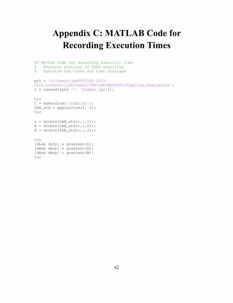
62

Appendix C: MATLAB Code for

Recording Execution Times

%% MATLAB Code for Recording Execution Time % Features portions of GSEG algorithm % Executed ten times and then averaged pth = 'C:\Users\jdw3970\HP-2012- 2013_svnroot\J_Whitesell\MATLAB(MASTER)\Pipeline_Si mulation' ; I = imread([pth '\' 'bigben.jpg' ]); tic C = makecform( 'srgb2lab' ); LAB_std = applycform(I, C); toc L = double(LAB_std(:,:,1)); A = double(LAB_std(:,:,2)); B = double(LAB_std(:,:,3)); tic [dLdx dLdy] = gradient(L); [dAdx dAdy] = gradient(A); [dBdx dBdy] = gradient(B); toc