1
The Courage of Misguided Convictions:The Trading Behavior of Individual Investors
Brad M. Barber∗[email protected]
www.gsm.ucdavis.edu/~bmbarber
Terrance Odean*[email protected]
www.gsm.ucdavis.edu/~odean
Graduate School of ManagementUniversity of California, Davis
Davis, CA, 95616-8609
July 1999
* We would like to thank Peter Klein, Hayne Leland, Richard Lyons, David Modest, John Nofsinger,James Poterba, Mark Rubinstein, Paul Ruud, Richard Sansing, Richard Thaler, Brett Trueman, andparticipants at the Berkeley Program in Finance, the NBER behavioral finance meetings, the Conference onHousehold Financial Decision Making and Asset Allocation at the Wharton School, the Western FinanceAssociation meetings, the Financial Management Association Conference, the Russell Sage Institute forBehavioral Economics, and seminar participants at UC Berkeley, the Yale School of Management, UCDavis, the University of Southern California, the University of North Carolina, Duke University, theWharton School, Stanford University, the University of Oregon, Harvard University, the MassachusettsInstitute of Technology, the Amos Tuck School, the University of Chicago, the University of BritishColumbia, Northwestern University, the University of Texas, UCLA, the University of Michigan, andColumbia University for helpful comments. We would also like to thank Jeremy Evnine and the discountbrokerage house which provided the data necessary for this study. Financial support from the NasdaqFoundation and the American Association of Individual Investors is gratefully acknowledged.

2
The Courage of Misguided Convictions:The Trading Behavior of Individual Investors
Modern financial economics assumes that we behave with extreme rationality; but, we do
not. Furthermore, our deviations from rationality are often systematic. Behavioral
finance relaxes the traditional assumptions of financial economics by incorporating these
observable, systematic, and very human departures from rationality into standard models
of financial markets. This paper highlights two common mistakes investors make; they
tend to disproportionately hold onto their losing investments while selling their winners
and they trade excessively. We argue that these systematic biases have their origins in
human psychology. The human desire to avoid regret causes investors to sell their
winners, while holding their losers; the tendency for human beings to be overconfident
prompts them to trade excessively.

1
There is one important caveat to the notion that we live in a new economy,
and that is human psychology… which appears essentially immutable.
Alan Greenspan
September 4, 1998
People do not always behave rationally. While departures from rationality are
sometimes random, often they are systematic. For example, far more people
overestimate, rather than underestimate, their driving ability (Svenson (1981)).
Behavioral models of financial markets consider not only how people should act, but how
they do act. Consideration for the observed traits of economic agents is not entirely new.
In 1738, Daniel Bernoulli noted that people behave as if they are risk-averse. Prior to
Bernoulli most scholars considered it normative behavior to value a gamble at its
expected value. Today economists usually assume people are risk-averse. Nineteenth
century economists believed that, ideally, the present and the future should be treated
equally; yet they observed that generally people value present consumption more highly
than future (Loewenstein (1992)). Today, economists usually assume that people discount
the utility of future consumption. In reality people are not always risk-averse nor do they
always discount the future. Millions of people engage in regular risk-seeking activity,
such as buying lottery tickets; others “bite the bullet” to get unpleasant experiences,
which they might otherwise delay, over with. However, risk-aversion and discounting
future consumption are sufficiently pervasive behaviors that they are standard
assumptions in economic models.
In recent years psychologists have identified ways in which people systematically
depart from optimal judgment and decision making. Behavioral finance enriches our
economic understanding by incorporating what we know about human nature into
financial models. Doing so is consistent with economic tradition, if not practice in
financial economics over the last several decades. Behavioral theories, like traditional
theories, provide formal hypotheses and predictions, which can be empirically tested.
This paper describes empirical tests of the predictions of two behavioral finance

2
theories. Shefrin and Statman (1985) extend the prospect theory of Kahneman and
Tversky (1979) to predict that investors will tend to hold their losing investments too
long and to sell their winners too soon; they label this tendency the disposition effect.
Odean (1998b) predicts that, due to their overconfidence, investors will trade too
frequently, thus reducing their returns. Many of the results presented here were first
reported in Odean (1998a), Odean (1999), and Barber and Odean (1999a, 1999b).
The next section describes the primary data for the tests reported in Sections 2 and
3. These data where first obtained for the purpose of testing the disposition effect. Section
2 reports the tests of the disposition effect. Section 3 reports tests of overconfidence and
excessive trading. In Section 4, we discuss more generally the motivations for the buying
and selling decisions of individual investors. We make concluding remarks in Section 5.
I. The DataA national discount brokerage house provided the data for the studies we
summarize. The primary dataset that we discuss is 10,000 randomly selected accounts
that were active in 1987 (those with at least one transaction). The data include trading and
position records for these accounts from January 1987 through December 1993. 162,948
trades are reported. Each record includes an account identifier, a buy-sell indicator, the
number of shares traded, the commission paid, and the principal amount.
Price and returns data are from the 1993 Center for Research in Security Prices
daily stock file for NYSE, AMEX, and Nasdaq stocks. The tests are limited to stocks for
which this information is available. Of the 10,000 accounts, 6,380 make 97,483 common
stock trades: 49,948 purchases and 47,535 sales. 62,516,332 shares are traded:
31,495,296 shares, with a market value of $530,719,264, are purchased and 31,021,036
shares, with a market value of $579,871,104 are sold. Average monthly turnover is 6.5
percent.1 The average size decile of a purchase is 8.65 and of a sale is 8.68, 10 being the
decile of the companies with the largest capitalization.
1 Turnover is estimated as one half the average monthly equity value of all trades (purchases and sales)divided by the average equity value of all monthly position statements.
3
II. The Disposition EffectThe disposition effect is one implication of extending Kahneman and Tversky's
(1979) prospect theory to investments. Under prospect theory, when faced with choices
involving simple two and three outcome lotteries, people behave as if maximizing an
“S”-shaped value function (see Figure 1). This value function is similar to a standard
utility function except that it is defined on gains and losses rather than on levels of
wealth. The function is concave in the domain of gains and convex in the domain of
losses. It is also steeper for losses than for gains, which implies that people are generally
risk-averse. Critical to this value function is the reference point from which gains and
losses are measured. Usually the status quo is taken as the reference point; however,
“there are situations in which gains and losses are coded relative to an expectation or
aspiration level that differs from the status quo.... A person who has not made peace with
his losses is likely to accept gambles that would be unacceptable to him otherwise”
(Kahneman and Tversky (1979)).
For example, suppose an investor purchases a stock that she believes to have an
expected return high enough to justify its risk. If the stock appreciates and the investor
continues to use the purchase price as a reference point, the stock price will then be in a
more concave, more risk-averse, part of the investor's value function. It may be that the
stock's expected return continues to justify its risk. However, if the investor somewhat
lowers her expectation of the stock's return, she will be likely to sell the stock. What if,
instead of appreciating, the stock declines? Then its price is in the convex, risk-seeking,
part of the value function. Here the investor will continue to hold the stock even if its
expected return falls lower than would have been necessary for her to justify its original
purchase. Thus the investor's belief about expected return must fall further to motivate
the sale of a stock that has already declined than one that has appreciated. Similarly,
consider an investor who holds two stocks. One is up; the other is down. If she is faced
with a liquidity demand, and has no new information about either stock, she is more
likely to sell the stock that is up.
Throughout this study, investors' reference points are assumed to be their
4
purchase prices. Though the results presented here appear to vindicate that choice, it is
likely that for some investments, particularly those held for a long time over a wide range
of prices, the purchase price may be only one determinant of the reference point. The
price path may also affect the level of the reference point. For example, a homeowner
who bought her home for $100,000 just before a real-estate boom and had the home
appraised for $200,000 after the boom, may no longer feel she is “breaking even” if she
sells her home for $100,000 plus commissions. If purchase price is a major component,
though not the sole component, of reference point, it may serve as a noisy proxy for the
true reference point. Using the proxy in place of the true reference point will make a case
for the disposition effect more difficult to prove. It seems likely that if the true reference
point were available the evidence reported here would be even stronger.
A. TaxesInvestors' reluctance to realize losses is at odds with optimal tax-loss selling for
taxable investments. For tax purposes investors should postpone taxable gains by
continuing to hold their profitable investments. They should capture tax losses by selling
their losing investments, though not necessarily at a constant rate. Constantinides (1984)
shows that when there are transactions costs, and no distinction is made between the
short-term and long-term tax rates (as is approximately the case from 1987 to 1993 for
U.S. federal taxes2), investors should gradually increase their tax-loss selling from
January to December. Dyl (1977), Lakonishok and Smidt (1986), and Badrinath and
Lewellen (1991) report evidence that investors do sell more losing investments near the
end of the year.
Shefrin and Statman (1985) propose that investors choose to sell their losers in
December as a self-control measure. They reason that investors are reluctant to sell for a
loss but recognize the tax benefits of doing so. The end of the year is the deadline for
2 Prior to 1987 long-term capital gains tax rates were 40 percent of the short-term capital gains tax rates;from 1987 to 1993 long-term and short-term gains were taxed at the same marginal rates for lower incometaxpayers. The maximum short-term rate at times exceeded the maximum long-term rate. In 1987 themaximum short-term rate was 38.5 percent and the maximum long-term rate was 28 percent. From 1988 to1990 the highest income taxpayers paid a marginal rate of 28 percent on both long-term and short-termgains. In 1991 and 1992 the maximum long-term and short term-rates were 28 percent and 31 percent. In1993 the maximum long-term and short-term rates were 28 percent and 39.6 percent.

5
realizing these losses. So each year, investors postpone realizing losses until December
when they require themselves to sell losers before the deadline passes.
B. MethodologyTo determine whether investors sell winners more readily than losers, it is not
sufficient to look at the number of securities sold for gains versus the number sold for
losses. Suppose investors are indifferent to selling winners or losers. Then in an upward-
moving market they will have more winners in their portfolios and will tend to sell more
winners than losers even though they had no preference for doing so. To test whether
investors are disposed to selling winners and holding losers, we must look at the
frequency with which they sell winners and losers relative to their opportunities to sell
each.
By going through each account's trading records in chronological order, a
portfolio of securities is constructed for which the purchase date and price are known.
Clearly this portfolio represents only part of each investor's total portfolio. In most
accounts there will be securities that were purchased before January 1987 for which the
purchase price is not available, and investors may also have other accounts that are not
part of the data set. Though the portfolios constructed from the data set are only part of
each investor's total portfolio, it is unlikely that the selection process will bias these
partial portfolios toward stocks for which investors have unusual preferences for realizing
gains or losses.
Each day that a sale takes place in a portfolio of two or more stocks, the selling
price for each stock sold is compared to its average purchase price to determine whether
that stock is sold for a gain or a loss. Each stock that is in that portfolio at the beginning
of that day, but is not sold, is considered to be a paper (unrealized) gain or loss (or
neither). Whether it is a paper gain or loss is determined by comparing its high and low
price for that day (as obtained from CRSP) to its average purchase price. If both its daily
high and low are above its average purchase price it is counted as a paper gain; if they are
both below its average purchase price it is counted as a paper loss; if its average purchase
price lies between the high and the low, neither a gain nor loss is counted. On days when

6
no sales take place in an account, no gains or losses, realized or paper, are counted.
In Table I we consider two investors: Randy and Naomi. Randy has five stocks in
his portfolio: A, B, C, D, and E. A and B are worth more than he paid for them; C, D, and
E are worth less. Another investor, Naomi, has three stocks in her portfolio: F, G, and H.
F and G are worth more than she paid for them; H is worth less. On Monday, Randy sells
shares of A and of C. Wednesday, Naomi sells shares of F. Randy's sale of A and
Naomi's sale of F are counted as realized gains. Randy's sale of C is a realized loss. Since
B and G could have been sold for a profit but weren't, they are counted as paper gains. D,
E, and G are paper losses. So, for these two investors over these two days, two realized
gains, one realized loss, two paper gains, and three paper losses are counted. Realized
gains, paper gains, realized losses, and paper losses are summed for each account and
across accounts. Then two ratios are calculated:
Proportion of Gains Realized (PGR) = Realized Gains
Realized Gains + Paper Gains
Proportion of Losses Realized (PLR) = Realized Losses
Realized Losses + Paper Losses
In the example of Randy and Naomi, PGR = 1/2 and PLR = 1/4. A large difference in the
proportion of gains realized (PGR) and the proportion of losses realized (PLR) indicates
that investors are more willing to realize either gains or losses.
Any test of the disposition effect is a joint test of the hypothesis that people sell
gains more readily than losses and of the specification of the reference point from which
gains and losses are determined. Some possible choices of a reference point for stocks are
the average purchase price, the highest purchase price, the first purchase price, or the
most recent purchase price. The findings of this study are essentially the same for each
choice; results are reported for average purchase price. Commissions and dividends may
or may not be considered when determining reference points, and profits and losses.
Although investors may not consider commissions when they remember what they paid
for a stock, commissions do affect capital gains and losses. And because the normative
7
standard to which the disposition effect is being contrasted is optimal tax-motivated
selling, commissions are added to the purchase price and deducted from the sales price in
this study except where otherwise noted. Dividends are not included when determining
which sales are profitable because they do not affect capital gains and losses for tax
purposes. The primary finding of these tests, that investors are reluctant to sell their losers
and prefer to sell winners, is unaffected by the inclusion or exclusion of commissions or
dividends. In determining whether the stocks that are not sold on a particular day could
have been sold for a gain or a loss, the commission for the potential sale is assumed to be
the average commission per share paid when the stock was purchased.3 All gains and
losses are calculated after adjusting for splits.
C. ResultsFigure 2 reports PGR and PLR for the entire year, for January through November,
and for December. We see that for the entire year investors do sell a higher proportion of
their winners than of their losers.
Suppose investors frequently realize small gains and less frequently take large
losses. It is then possible that they are selling similar proportions of the values of their
gains and losses, though realizing gains at a higher rate on a trade-counted basis. This is,
however, not the case. The average PGR and PLR per account can be calculated by
measuring losses, gains, potential losses, and potential gains in terms of dollars rather
than shares or trades. The dollar-based PGR (averaged across accounts) is 0.58 and the
average dollar-based PLR (averaged across accounts) is 0.42.4
In Figure 2 the ratio of PGR to PLR for the entire year is a little over 1.5,
indicating that a stock that is up in value is over 50 percent more likely to be sold from
day to day than a stock that is down. In Weber and Camerer's (1995) experimental studies
of the disposition effect, a stock that is up is also about 50 percent more likely to be sold
3 If, for potential sales, the commission is instead assumed to be the same percentage of principal as paidwhen the stock was purchased, the results do not significantly change.4 It should be noted that the PGR and the PLR measures are dependent on the average size of the portfoliosfrom which they are calculated. When the portfolio sizes are small and when average account proportions,rather than aggregate sample proportions are calculated, both of these proportions tend to be larger.

8
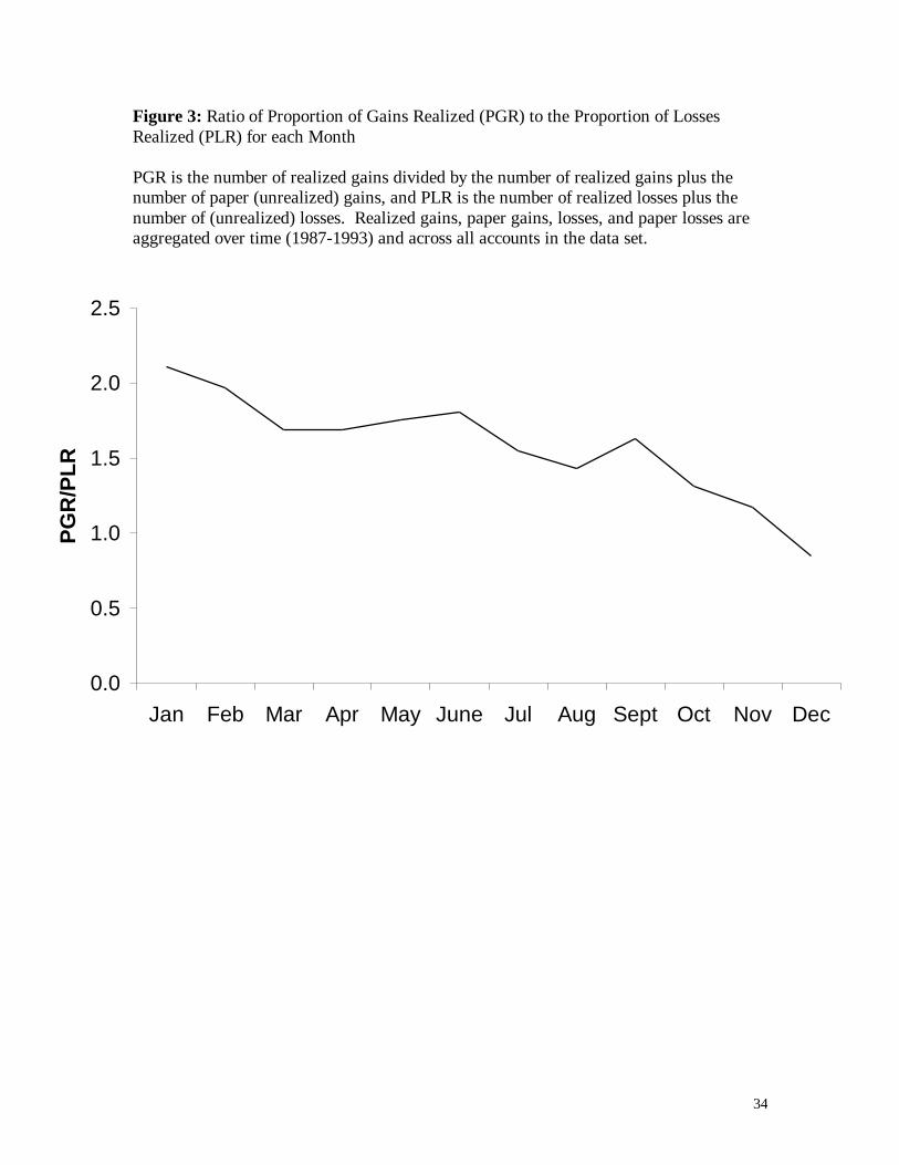
than one that is down. Figure 3 charts the ratio of PGR to PLR for each month. This ratio
declines from 2.1 in January to 0.85 in December. This decline is consistent with
Constantinides' tax-loss selling model and suggests that at least some investors pay
attention to tax-motivated selling throughout the year. From January through November,
however, the observed ratio of PGR to PLR is reliably greater than 1.5
It is worth emphasizing that the results described here hold up to a classic
principle of scientific inquiry; they are robust to out-of-sample testing. Specifically,
subsequent to Odean (1998a), we obtained trading records for 78,000 households from
1991 to 1996 from the same discount brokerage house. (These data are described in more
detail in Section IV.D.) For this new dataset, the PGR measure is 0.1442 and the PLR
measure is 0.0863. During this sample period, stocks that had increased in value were
approximately 65 percent more likely to be sold than stocks that had declined in value.
D. Alternative Reasons to Hold Losers and Sell WinnersPrevious research6 offers some support for the hypothesis that investors sell
winners more readily than losers, but this research is generally unable to distinguish
among various motivations investors might have for doing so. Recent studies have found
5 In the reported PLR and PGR calculations, realized and unrealized losses are tabulated on days that salestook place in portfolios of two or more stocks. One objection to this formulation is that for portfolios thathold only winners or only losers an investor cannot choose whether to sell a winner or to sell a loser, butonly which winner or loser to sell. Another objection is that if an investor has net capital losses of morethan $3,000 for the current year (in non-tax-deferred accounts) if may be normative for that investor tochoose to sell a winner rather than a loser. The analyses reported in the tables were repeated subject to theadditional constraints that there be at least one winner and one loser in a portfolio on the day of a sale forthat day to be counted and that the net realized capital losses for the year to date in the portfolio be less than$3,000. When these constraints are imposed, the difference in PGR and PLR is, for each analysis, greater.For example, for the entire sample and the entire year (as in Figure 2) there are 10,111 realized gains,71,817 paper gains, 5,977 realized losses, and 94,419 paper losses. Thus the PLR is 0.060; the PGR is0.123; their difference is 0.063; and the t-statistic for the difference in proportions is 47.6 Starr-McCluer (1995) finds that 15 percent of the stock-owning households interviewed in the 1989 and1992 Surveys of Consumer Finances have paper losses of 20 percent or more. She estimates that in themajority of cases the tax advantages of realizing these losses would more than offset the trading costs andtime costs of doing so. Heisler (1994) documents loss aversion in a small sample of futures speculators. Ina study of individual federal tax returns, Poterba (1987) finds that although many investors do offset theircapital gains with losses, more than 60 percent of the investors with gains or losses realized only gains.Weber and Camerer (1995) report experimental evidence of the disposition effect. Lakonishok and Smidt(1986) and Ferris, Haugen, and Makhija (1988) find a positive correlation between price change andvolume. Bremer and Kato (1996) find the same correlation for Japanese stocks. Such a correlation could becaused by investors who prefer to sell winners and hold losers, but it could also be the result of buyers'trading preferences.

9
evidence of the disposition effect in the exercise of company stock options (Heath,
Huddart, and Lang (1999)), residential housing (Genesove and Mayer (1999)),
professional futures traders (Locke and Mann (1999)), and Finnish investors (Grinblatt
and Keloharju (1999)). We believe the disposition effect best explains the tendency for
investors to hold losers and sell winners. In this section, we present evidence that allow
us to discount competing explanations for this investor behavior.
D.1. Anticipation of Changes in Tax LawOne reason investors might choose to sell winners rather than losers is that they
anticipate a change in the tax law under which capital gains rates will rise. The tax law of
1986 made such a change. If investors sold off winners in anticipation of higher tax rates,
they might have entered 1987 with a larger percentage of losers in their portfolio than
usual. Because such stocks are purchased prior to 1987 they would not show up in the
portfolios reconstructed here. It is possible therefore that the rate at which winners are
being realized relative to losers is lower in the investors' total portfolio than in the partial
reconstructed portfolios. As old stocks are sold and new ones purchased the partial
portfolios become more and more representative of the total portfolio. We would expect
that if a sell-off of winners in anticipation of the 1986 tax law affects the observed rate at
which gains and losses are realized in the partial portfolios, that effect would be greater in
the first part of the sample period than in the last part. However the ratio PGR/PLR is
virtually the same for the periods 1987 to 1990 and 1991 to 1993.
D.2. Desire to RebalanceLakonishok and Smidt (1986) suggest that investors might sell winners and hold
on to losers in an effort to rebalance their portfolios. Investors who sell winners for the
purpose of rebalancing their portfolios are likely to make new purchases. To eliminate
trades that may be motivated by a desire to rebalance, PGR and PLR are calculated using
only sales and dates for which there is no new purchase into a portfolio on the sale date or
during the following three weeks. When sales motivated by a desire to rebalance are
eliminated in this way, investors continue to prefer to sell winners. Once again, investors
realize losses at a higher rate than gains in December.

10
D.3. Belief that One's Losers Will Bounce BackAnother reason investors might sell winners and hold losers is that they expect
their losers to outperform their winners in the future. An investor who buys a stock
because of favorable information may sell that stock when it goes up because she
believes her information is now reflected in the price. On the other hand, if the stock goes
down she may continue to hold it, believing that the market has not yet come to
appreciate her information. Investors could also choose to sell winners and hold losers
simply because they believe prices mean revert. It is possible to test whether such beliefs
are justified, ex post.
To test whether losing stocks investors continue to hold outperform winners that
they sell, Odean (1998a) calculates market-adjusted returns for losing stocks held and
winning stocks sold subsequent to each sales date. For winners that were sold, he
calculates market-adjusted returns (the average return in excess of the CRSP value
weighted index) starting the day after the transaction for the next 84 trading days (four
months), 252 trading days (one year), and 504 trading days (two years). For the same
horizons, he calculates market-adjusted returns subsequent to paper losses. That is, for
stocks held for a loss in portfolios on which sales did take place, market-adjusted returns
are calculated starting the day after the sale for the next 84, 252, and 504 trading days.
For winners that are sold, the average excess return over the following year is a highly
statistically significant 3.4 percent more than it is for losers that are not sold.7 (Winners
sold subsequently outperform paper losses by 1.03 percent over the following four
months and 3.58 percent of the following two years.) Investors who sell winners and hold
losers because they expect the losers to outperform the winners in the future are, on
average, mistaken. The superior returns to former winners noted here are consistent with
Jegadeesh and Titman's (1993) finding of price momentum in security returns at horizons
of up to eighteen months.8
7 Here and in Section 3, statistical significance is determined using a bootstrapping technique similar tothose discussed in Brock, Lakonishok, and LeBaron (1992), Ikenberry, Lakonishok, and Vermaelen (1995),and Lyon, Barber, and Tsai(1999). This procedure described in greater detail in Odean (1998a) and Odean(1999).8 At the time of this study CRSP data were available through 1994. For this reason two-year subsequentreturns are not calculated for sales dates in 1993.

11
D.4. Attempt to Limit Transaction CostsHarris (1988) suggests that investors' reticence to sell losers may be due to their
sensitivity to higher trading costs at lower stock prices. To contrast the hypothesis that
losses are realized more slowly due to the higher transactions costs with the disposition
effect, we can look at the rates at which investors purchase additional shares of stocks
they already own. If investors are avoiding the sale of losing investments because of the
higher transaction costs associated with selling low price stocks, we would also expect
them to avoid purchasing additional shares of these losing investments. In fact, this is not
the case; investors are more inclined to purchase additional shares of their losing
investments than additional shares of their winning investments. In this sample, investors
are almost one and one half times as likely to purchase additional shares of any losing
position they already hold than any winning position.
D.5. Belief that All Stocks Mean RevertThe results presented so far are not able to distinguish prospect theory and the
mistaken belief that losers will bounce back to outperform current winners. Both prospect
theory and a belief in mean reversion predict that investors will hold their losers too long
and sell their winners too soon. Both predict that investors will purchase more additional
shares of losers than of winners. However a belief in mean reversion should apply to
stocks that an investor does not already own as well as those she does, but prospect
theory applies only to the stocks one owns. Thus a belief in mean reversion implies that
investors will tend to buy stocks that had previously declined even if they don't already
own these stocks, while prospect theory makes no prediction in this case. Odean (1999)
finds that this same group of investors tends to buy stocks that have, on average,
outperformed the CRSP value-weighted index by about 25 percent over the previous two
years. This would appear inconsistent with a pervasive belief in mean reversion.
III. Overconfidence and Excessive TradingIt is difficult to reconcile the volume of trading observed in equity markets with
the trading needs of rational investors. Rational investors make periodic contributions and
withdrawals from their investment portfolios, rebalance their portfolios, and trade to
minimize their taxes. Those possessed of superior information may trade speculatively,
though rational speculative traders will generally not choose to trade with each other. It is
12
unlikely that rational trading needs account for a turnover rate of 76 percent on the New
York Stock Exchange in 1998.
We believe there is a simple and powerful explanation for high levels of trading
on financial markets: overconfidence. Human beings are overconfident about their
abilities, their knowledge, and their future prospects. Odean (1998) shows that
overconfident investors trade more than rational investors and that doing so lowers their
expected utilities. Greater overconfidence leads to greater trading and to lower expected
utility.
Overconfidence increases trading activity because it causes investors to be too
certain about their own opinions and to not consider sufficiently the opinions of others.
This increases the heterogeneity of investors beliefs -- the source of most trading.
Overconfident investors also perceive their actions to be less risky than generally proves
to be the case.
The study reported in this section tests whether a particular class of investors,
those with accounts at discount brokerages, trade excessively in the sense that their
trading profits are insufficient to cover their trading costs. The surprising finding is that,
not only do the securities that these investors buy not outperform the securities they sell
by enough to cover trading costs, but on average the securities they buy underperform
those they sell. This is the case even when trading is not apparently motivated by
liquidity demands, tax-loss selling, portfolio rebalancing, or a move to lower-risk
securities. While investors' overconfidence in the precision of their information may
contribute to this finding, it is not sufficient to explain it. These investors must be
systematically misinterpreting information available to them. They do not simply
misconstrue the precision of their information, but its very meaning.
A. OverconfidenceStudies of the calibration of subjective probabilities find that people tend to
overestimate the precision of their knowledge (Alpert and Raiffa (1982), Fischhoff,
Slovic and Lichtenstein (1977); see Lichtenstein, Fischhoff, and Phillips (1982) for a
13
review of the calibration literature). Such overconfidence has been observed in many
professional fields. Clinical psychologists (Oskamp (1965)), physicians and nurses,
(Christensen-Szalanski and Bushyhead (1981), Baumann, Deber, and Thompson (1991)),
investment bankers (Staël von Holstein (1972)), engineers (Kidd (1970)), entrepreneurs
(Cooper, Woo, and Dunkelberg (1988)), lawyers (Wagenaar and Keren (1986)),
negotiators (Neale and Bazerman (1990)), and managers (Russo and Schoemaker (1992))
have all been observed to exhibit overconfidence in their judgments. (For further
discussion, see Lichtenstein, Fischhoff, and Phillips (1982) and Yates (1990).)
Miscalibration is only one manifestation of overconfidence. Researchers also find
that people overestimate their ability to do well on tasks and these overestimates increase
with the personal importance of the task (Frank (1935)). People are also unrealistically
optimistic about future events. They expect good things to happen to them more often
than to their peers (Weinstein (1980); Kunda (1987)). They are even unrealistically
optimistic about pure chance events (Marks (1951), Irwin (1953), Langer and Roth
(1975)).
People have unrealistically positive self-evaluations (Greenwald (1980)). Most
individuals see themselves as better than the average person and most individuals see
themselves better than others see them (Taylor and Brown (1988)). They rate their
abilities and their prospects higher than those of their peers. For example, when a sample
of U.S. students -- average age 22 -- assessed their own driving safety, 82 percent judged
themselves to be in the top 30 percent of the group (Svenson (1981)). And 81 percent of
2994 new business owners thought their business had a 70 percent or better chance of
succeeding but only 39 percent thought that any business like theirs would be this likely
to succeed (Cooper, Woo, and Dunkelberg (1988)). People overestimate their own
contributions to past positive outcomes, recalling information related to their successes
more easily than that related to their failures. Fischhoff (1982) writes that “they even
misremember their own predictions so as to exaggerate in hindsight what they knew in
foresight.” And when people expect a certain outcome and the outcome then occurs, they
often overestimate the degree to which they were instrumental in bringing it about (Miller

14
and Ross (1975)). Taylor and Brown (1988) argue that exaggerated beliefs in one's
abilities and unrealistic optimism may lead to “higher motivation, greater persistence,
more effective performance, and ultimately, greater success.” These beliefs can also lead
to biased judgments.
B. Overconfidence in Financial MarketsIn a market with transaction costs we would expect rational informed traders who
trade for the purpose of increasing returns to increase returns, on average, by at least
enough to cover transaction costs. That is, over the appropriate horizon, the securities
these traders buy will outperform the ones they sell by at least enough to pay the costs of
trading. If speculative traders are informed, but overestimate the precision of their
information (one form of overconfidence), the securities they buy will, on average,
outperform those they sell, but possibly not by enough to cover trading costs. If these
traders believe they have information, but actually have none, the securities they buy will,
on average, perform about the same as those they sell before factoring in trading costs.
Overconfidence in only the precision of unbiased information will not, in and of itself,
cause expected trading losses beyond the loss of transactions costs.
If in addition to being overconfident about the precision of their information,
investors are overconfident about their ability to interpret information, they may incur
average trading losses beyond transactions costs. Suppose investors receive useful
information but are systematically biased in their interpretation of that information; that
is, the investors hold mistaken beliefs about the mean, instead of (or in addition to) the
precision of the distribution of their information. If they unwittingly misinterpret
information, they may choose to buy or sell securities which they would not have
otherwise bought or sold. They may even buy securities that, on average and before
transaction costs, underperform the ones they sell.
C. MethodologyTo test for overconfidence in the precision of information, it is determined
whether the securities investors in this dataset buy outperform those they sell by enough
to cover the costs of trading. To test for biased interpretation of information, it is
15
determined whether the securities they buy underperform those they sell when trading
costs are ignored. Return horizons of four months (84 trading days), one year (252
trading days), and two years (504 trading days) following each transaction are examined.9
Returns are calculated from the CRSP daily return files.
To calculate the average return to securities bought (sold) in these accounts over
the T (T=84, 252, or 504) trading days subsequent to the purchase (sale), each purchase
(sale) transaction is indexed with a subscript i, i=1 to N. Each transaction consists of a
security, ji, and a date, ti. If the same security is bought (sold) in different accounts on the
same day, each purchase (sale) is treated as a separate transaction. Market-adjusted
returns are calculated as the security return less the return on the CRSP value-weighted
index. The market-adjusted return for the securities bought over the T trading days
subsequent to the purchase is:
RN
R RP T j t
T
VW t
T
i
N
i i i, , ,= + − +FHG
IKJ+
=+
==∏ ∏∑1
1 11 11
ττ
ττ
d i d iWhere Rj,t is the CRSP daily return for security j on date t and RVW,t is the daily return for
the CRSP value-weighted index on date t. Note that return calculations begin the day
after a purchase or a sale so as to avoid incorporating the bid-ask spread into returns.
In this dataset, the (equally weighted) average commission paid when a security is
purchased is 2.23 percent of the purchase price. The average commission on a sale is 2.76
percent of the sale price.10 Thus if one security is sold and the sale proceeds are used to
buy another security the total commissions for the sale and purchase average about 5
percent. The average effective bid-ask spread is 0.94 percent.11 Thus the average total
cost of a round-trip trade is about 5.9 percent. An investor who sells securities and buys
others because he expects the securities he is buying to outperform the ones he is selling, 9 Investment horizons will vary among investors and investments. Benartzi and Thaler (1995) estimate theaverage investor's investment horizon to be one year, and, during this period, NYSE securities turned overabout once every two years. At the time of this analysis CRSP data was available through 1994. For thisreason two year subsequent returns are not calculated for transactions dates in 1993.10 Weighting each trade by its equity value, rather than equally, the average commission for a purchase(sale) is 0.9 (0.8) percent.
16
will have to realize, on average and weighting trades equally, a return nearly 6 percent
higher on the security he buys just to cover trading costs.
The first hypothesis tested here is that, over horizons of four months, one year,
and two years, the average returns to securities bought minus the average returns to
securities sold are less than the average round-trip trading costs of 5.9 percent. This is
what we expect if investors are sufficiently overconfident about the precision of their
information. The null hypothesis (N1) is that this difference in returns is greater than or
equal to 5.9 percent. The null is consistent with rationality. The second hypothesis is that
over these same horizons the average returns to securities bought are less than those to
securities sold, ignoring trading costs. This hypothesis implies that investors must
actually misinterpret useful information. The null hypothesis (N2) is that average returns
to securities bought are greater than or equal to those sold.
D. ResultsTable II, Panel A reports results for all purchases and all sales of stocks in the
database. For all three follow-up periods the average subsequent market-adjusted returns
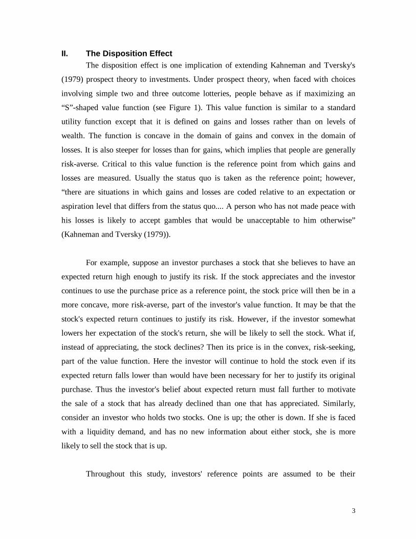
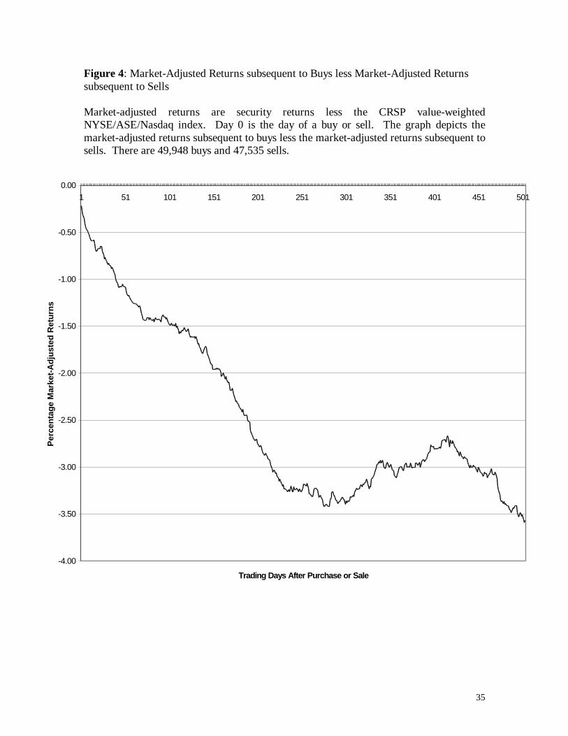
to stocks which were bought is less than that to stocks which were sold. Figure 4
provides a graph of the difference between the market-adjusted returns to stocks that
were bought and the market-adjusted returns to stocks that were sold. Regardless of the
horizon, the stocks that investors bought underperformed the stocks that they sold. (This
is also true when actual returns are calculated instead of market-adjusted returns). Not
only do the investors pay transactions costs to switch stocks, but the stocks they buy
underperform the ones they sell. For example, for the entire sample over a one year
horizon the average market-adjusted return on a purchased stock is 3.2 percent lower than
the average market-adjusted return on a stock sold.
The null hypothesis that the expected returns to stocks purchased are 5.9 percent
(the average cost of a round trip trade) or more greater than the expected returns to stocks
sold is comfortably rejected (p < 0.001). The second null hypothesis, that the expected 11 Barber and Odean (1999a) estimate the bid-ask spread of 1.00 percent for individual investors from 1991to 1996. Carhart (1997) estimates trading costs of 0.21 per cent for purchases and 0.63 per cent for sales

17
returns to stocks purchased are greater than or equal to those of stocks sold (ignoring
transactions costs), is also comfortably rejected (p-values less then 0.002 depending on
the horizon).
These investors are not making profitable trades. Of course investors trade for
reasons other than to increase profit. They trade to meet liquidity demands. They trade to
move to more, or to less, risky investments. They trade to realize tax-losses. And they
trade to rebalance; for example if one stock in her portfolio appreciates considerably, an
investor may sell part of her holding in that stock and buy others to rebalance her
portfolio. Panel B examines trades for which these alternative motivations to trades have
been largely eliminated. This panel examines only sales and purchases where a purchase
was made within three weeks of a sale; such transactions are unlikely to be liquidity
motivated since investors who need cash for three weeks or less can borrow more cheaply
(e.g. using credit cards) than the cost of selling and later buying stocks. All of the sales in
this panel were for a profit; so these stocks were not sold in order to realize tax-losses
(and they were not short sales). These sales were of an investor's complete holding in the
stock sold; so most of these sales were not motivated by a desire to rebalance the
holdings of an appreciated stock. Also this panel examines only sales and purchases
where the purchased stock is from the same size decile as the stock sold or it is from a
smaller size decile (CRSP size deciles for the year of the transaction); since size has been
shown to be highly correlated with risk, this restriction is intended to eliminate most
instances where an investor intentionally buys a stock of lower expected return than the
one he sells because he is hoping to reduce his risk.
We see in Panel B that when all of these alternative motivations for trading are
eliminated, investors actually perform worse over all three evaluation periods; over a one
year horizon the stocks these investors sell underperform those they buy by about 5
percent. Sample size is, however, greatly reduced and statistical significance slightly
lower. Nonetheless, both null hypotheses can still be comfortably rejected.
made by open-end mutual funds from 1966 to 1993.

18
As was the case for the tests of the disposition effect, we have been able to
replicate these results out-of-sample. Subsequent to Odean (1999), we obtained trading
records for 78,000 households from 1991 to 1996 from the same discount brokerage
house. (These data are described in more detail in Section IV.E.) On average, the
1,082,106 stocks that these households buy reliably underperform (p<0.001) the 887,638
they sell by 2.35 percent over the 252 trading days subsequent to each transaction.
Overconfidence alone cannot explain these results. These investors appear to have
some ability to distinguish stocks that will subsequently perform better and worse.
Unfortunately, somehow they get the relationship wrong. In part, this may lie in the
differences in how they choose which stocks to buy and which to sell.
E. Additional Tests of Overconfidence
E.1. Turnover and PerformanceOdean (1998b) predicts that the more overconfident investors are the more they
will trade and the more they will thereby lower their expected utilities. If overconfidence
is an important motivation for investor trading, then we would expect that, on average,
those investors who trade most actively will most reduce their returns through trading. As
reported in Barber and Odean (1999a), we find that this is the case.
We examine trading and position records for 78,000 households with accounts at
the same discount brokerage house as supplied the data described above. The records are
from January 1991 through December 1996 and include all accounts at this brokerage for
each household. (See Barber and Odean (1999a) for a detailed description of these data.)
Of the 78,000 sampled households, 66,465 had positions in common stocks during at
least one month; the remaining accounts either held cash or investments in other than
individual common stocks. Roughly 60 percent of the market value in the accounts was
held in common stocks. There were over 3 million trades in all securities; common
stocks accounted for slightly more than 60 percent of all trades. In December 1996, these
households held more than $4.5 billion in common stock. In addition to trade and
position records, for much of our sample, our dataset identifies demographic

19
characteristics such as age, gender, marital status, and income.
We partition the households into quintiles on the basis of the average monthly
turnover of their common stock portfolios. Mean monthly turnover for these quintiles
ranges from 0.19 percent (low turnover quintile) to 21.49 percent (high turnover quintile).
Households that trade frequently (high turnover quintile) earn a net annualized geometric
mean return of 11.4 percent, while those that trade infrequently (low turnover quintile)
earn 18.5 percent. Because the households in each quintile may (and do) vary in their
average risk characteristics of their portfolios, we compare the annual net return earned
by each household to the annual net return that would have been earned had the
household's beginning of the year portfolio been held for a year without any trading. This
is a reasonable measure of the impact of trading on returns. The quintile of households
that trade most infrequently underperform their “buy-and-hold” portfolios, on average, by
a mere 0.25 percent annually, while the quintile of households that trade most frequently
underperform their “buy-and-hold” portfolios, on average, by 7.04 percent annually.
Our finding that the more investors trade the more they reduce their expected
returns is consistent with the prediction that more overconfident traders will trade more
actively and earn less. However, we still haven't tested directly whether overconfidence is
motivating trading. To do so, we partition our data into two groups which psychologists
have shown to differ in their tendency to overconfidence: men and women.
E.2. Gender, Overconfidence and PerformanceWhile both men and women exhibit overconfidence, men are generally more
overconfident than women (Lundeberg, Fox, and Puncochar (1994)).12 Gender
differences in overconfidence are highly task dependent (Lundeberg, Fox, and Puncochar
(1994)). Deaux and Ferris (1977) write “Overall, men claim more ability than do women,
but this difference emerges most strongly on … masculine task[s].” Several studies
confirm that differences in confidence are greatest for tasks perceived to be in the
masculine domain (Deaux and Emswiller (1994), Lenney (1977), Beyer and Bowden

20
(1997)). Men are inclined to feel more competent than women do in financial matters
(Prince (1993)). Indeed, casual observation reveals that men are disproportionately
represented in the financial industry. We expect, therefore, that men will generally be
more overconfident about their ability to make financial decisions than women.
Additionally, Lenney (1977) reports that gender differences in self-confidence
depend on the lack of clear and unambiguous feedback. When feedback is “unequivocal
and immediately available, women do not make lower ability estimates than men.
However, when such feedback is absent or ambiguous, women seem to have lower
opinions of their abilities and often do underestimate relative to men.” The stock market
does not generally provide clear unambiguous feedback. All the more reason to expect
men to be more confident than women about their ability to make common stock
investments.
Our prediction, then, is clear: we expect men, the more overconfident group, to
trade more actively than women and, in doing so, to detract from their net return
performance more. As reported in Barber and Odean (1999b), we find that this prediction
holds true. Men trade 45 percent more actively than do women (76.9 percent turnover
annually versus 52.8 percent). And men reduce their net annual returns through trading
by 0.94 percent more than do women. (Men underperform their “buy-and-hold”
portfolios by 2.652 percent annually; women underperform their “buy-and-hold”
portfolios by 1.716 percent annually.) The differences in the turnover and performance of
men and women are highly statistically significant and robust to the introduction of other
demographic variables such as marital status, age, and income.
IV. Buying vs. SellingOur analysis of the trading behavior of individual investors reveals that most
investors treat the decision to buy a security quite differently from the decision to sell. On
the one hand, consider the selling behavior of individual investors. Since most investors
don't short -- less than 1 percent of the sales in the datasets are short sales -- those seeking 12 While Lichtenstein and Fishhoff (1981) do not find gender differences in calibration of generalknowledge, Lundeberg, Fox, and Puncochar (1994) argue that this is because gender differences in
21
a security to sell need only consider the ones they already own. This is usually a
manageable handful; in both datasets the average number of securities, including bonds,
mutual funds, and options as well as stocks, per account is less than 7. Investors can
carefully consider selling each security they own regardless of the attention given it in the
media.
Though the search for securities to sell is simple, in other respects the decision to
sell a security is more complex than the decision to buy. When choosing securities to
buy, an investor only needs to form expectations about the future performance of those
securities. When choosing securities to sell, the investor will consider past as well as
future performance. If the investor is rational he will want to balance the advantages or
disadvantages of any tax losses or gains he realizes from a sale against future returns he
expects a security to earn. If an investor is psychologically motivated he may wish to
avoid realizing losses and prefer to sell his winners, as do the majority of the investors
studied here, and this psychological motivation for sales generally dominates tax-
motivated sales. Thus, ceterus paribus, securities that have appreciated in value become
candidates for a sale.
On the other hand, consider the buying behavior of individual investors. Investors
face a formidable challenge when looking for a security to buy. There are well over
10,000 securities to be considered. These investors do not have a retail broker available to
suggest purchase prospects. While the search for potential purchases can be simplified by
confining it to a subset of all securities (e.g., the S&P 500) even then, the task of
evaluating and comparing each security is beyond what most non-professionals are
equipped to do. Unable to evaluate each security, investors are likely to consider
purchasing securities to which their attention has been drawn. Investors may think about
buying securities they have recently read about in the paper or heard about on the news.
Securities that have performed unusually well or poorly are more likely to be discussed in
the media, more likely to be considered by individual investors, and ultimately, more
likely to be purchased. Odean (1999) finds that these investors tend to buy stocks with
calibration are strongest for topics in the masculine domain.

22
recent returns of greater absolute value than the stocks they sell.
Once their attention has been directed to potential purchases, investors vary in
their propensity to buy previous winners or previous losers.13 It may be that those who
buy previous winners believe that securities follow trends, while those who buy previous
losers believe they revert. The investors who believe in trend may buy previous winners
to which their attention has been directed, while those who believe in reversion buy
previous losers to which their attention has been directed. If investors were as willing to
sell securities short as to buy, we might expect them to actively sell as well as to actively
buy securities to which their attention was directed. But, for the most part, these investors
do not sell short.
V. ConclusionOne of the major contributions of behavioral finance is that it provides insights
into investor behavior where such behavior cannot be understood using traditional
theories. In this paper we test two behavioral finance theories. As predicted, we find that
investors tend to sell their winning stocks and to hold on to their losers and that, as a
result of overconfidence, investors trade too much. These behaviors reduce investor
welfare. Understanding these behaviors is therefore important for investors and for those
who advise them.
But the welfare consequences of investor behavior extend beyond individual
investors and their advisors. Modern financial markets depend on trading volume for
their very existence. It is trading -- commissions and spreads -- that pays for the brokers
and market-makers without whom these markets would not exist. Traditional models of
financial markets give us very little insight into why people trade as much as they do. In
some models investors hardly trade, or don't trade at all (e.g., Grossman (1976)). Other
models simply stipulate a class of investors -- noise or liquidity traders -- that are
required to trade (e.g., Kyle (1985)). Harris and Raviv (1993) and Varian (1989) point out
that heterogeneous beliefs are needed to generate significant trading. But it is behavioral
13 Odean (1999) rejects the hypothesis that the probability of buying previous winners (or losers) is thesame for all investors in the dataset described above.
23
finance that gives us insights into why and when investors form heterogeneous beliefs.
Both of the behavioral theories tested in this paper offer insights into trading
volume. The disposition effect says that investors will generally trade less actively when
their investments have lost money. The overconfidence theory suggests that investors will
trade more actively when their overconfidence is high. Psychologists find that people
tend to give themselves too much credit for their own success and do not attribute enough
of that success to chance or outside circumstance. Gervais and Odean (1999) show that
this bias leads successful investors to become overconfident. And, in a market where
most investors are successful (e.g., a long bull market), aggregate overconfidence and
consequent trading rise. Statman and Thorley (1999) find that over even short horizons,
such as a month, current market returns predict subsequent trading volume.
In the last two decades researchers have discovered many anomalies that
apparently contradict established finance theories.14 New theories, both behavioral (e.g.,
(Barberis, Shleifer, and Vishny (1997), Daniel, Hirshleifer, and Subrahmanyam (1998))
and rational (e.g., Berk (1995)) have been devised to explain anomalies in asset prices. It
is not yet clear what contribution behavioral finance will make to asset pricing theory.
The investor behaviors discussed in this paper have the potential to influence asset
prices. The tendency to refrain from selling losing investments may, for example, slow
the rate at which negative news is impacted into price. The tendency to buy stocks with
recent extreme performance could cause recent winners to overshoot. For biases to
influence asset prices, investors must be sufficiently systematic in their biases and
sufficiently willing to act on them.15
Our common psychological heritage insures that we systematically share biases.
Overconfidence provides the will to act. It gives us the courage of our misguided
convictions.
14 See, for example, Thaler's (1992) collection of “Anomalies” articles originally published in the Journalof Economic Perspectives.15 Of course, there must also be limits to arbitrage (see Shleifer and Vishny (1998)).
24
References
Alpert, Marc, and Howard Raiffa, 1982, A progress report on the training of probabilityassessors, in Daniel Kahneman, Paul Slovic, and Amos Tversky, eds.: JudgmentUnder Uncertainty: Heuristics and Biases, (Cambridge University Press,Cambridge and New York).
Badrinath, S., Lewellen, Wilber., 1991, Evidence on tax-motivated securities tradingbehavior, Journal of Finance, 46, 369-382.
Barber, Brad M., and Terrance Odean, 1999a, Trading is hazardous to your wealth: Thecommon stock investment performance of individual investors, forthcomingJournal of Finance.
Barber, Brad M., and Terrance Odean, 1999b, Boys will be boys: Gender,overconfidence, and common stock investment, Working paper, University ofCalifornia, Davis.
Barberis, Nicholas, Andre, Shleifer, and Robert Vishny, 1996, A model of investorsentiment with both underreaction and overreaction, Working paper, University ofChicago.
Baumann, Andrea O., Raisa B. Deber, and Gail G. Thompson, 1991, Overconfidenceamong physicians and nurses: The “Micro-Certainty, Macro-Uncertainty”Phenomenon, Social Science \& Medicine, 32, 167-174.
Benartzi, Shlomo, and Richard Thaler, 1995, Myopic loss aversion and the equitypremium puzzle, Quarterly Journal of Economics, 110, 73-92.
Berk, Jonathan, 1995, A critique of size related anomalies, Review of Financial Studies,,8, 275-286.
Bremer, Marc, and Kato Kiyoshi, 1996, Trading volume for winners and losers on theTokyo Exchange, Journal of Financial and Quantitative Analysis, 31, 127-142.
Beyer, Sylvia, and Edward M.Bowden, 1997, Gender differences in self-perceptions:Convergent evidence from three measures of accuracy and bias, Personality andSocial Psychology Bulletin, 23, 157-172.
Brock, William, Josef Lakonishok, and Blake LeBaron, 1992, Simple technical tradingrules and the stochastic properties of stock returns, Journal of Finance, 47, 1731-1764.
Carhart, Mark M., 1997, On persistence in mutual fund performance, Journal of Finance,52, 57-82.

25
Christensen-Szalanski, Jay J., and James B. Bushyhead, 1981, Physicians' use ofprobabilistic information in a real clinical setting, Journal of ExperimentalPsychology: Human Perception and Performance, 7, 928-935.
Constantinides, George, 1984, Optimal stock trading with personal taxes: Implicationsfor prices and the abnormal January returns, Journal of Financial Economics, 13,65-69.
Cooper, Arnold C., Carolyn Y. Woo, and William C. Dunkelberg, 1988, Entrepreneurs'perceived chances for success, Journal of Business Venturing, 3, 97-108.
Deaux, Kay, and Tim Emswiller, 1974, Explanations of successful performance on sex-linked tasks: What is skill for the male is luck for the female, Journal ofPersonality and Social Psychology, 29, 80-85.
Deaux, Kay, and Elizabeth Farris, 1977, Attributing causes for one's own performance:The effects of sex, norms, and outcome, Journal of Research in Personality, 11,59-72.
Daniel, Kent, David Hirshleifer, and Avanidhar Subrahmanyam, 1998, A Theory ofOverconfidence, Self-Attribution, and Security Market Under- and Over-Reactions, Journal of Finance, 53, 1839-1886.
Dyl, Edward, 1977, Capital gains taxation and the year-end stock market behavior,Journal of Finance, 32, 165-175.
Ferris, Stephen, Robert Haugen, and Anil Makhija, 1988, Predicting contemporaryvolume with historic volume at differential price levels: Evidence supporting thedisposition effect, Journal of Finance, 43, 677-697.
Fischhoff, Baruch, 1982, For those condemned to study the past: Heuristics and biases inhindsight, in Daniel Kahneman, Paul Slovic, and Amos Tversky, eds.: JudgmentUnder Uncertainty: Heuristics and Biases, (Cambridge University Press,Cambridge and New York).
Fischhoff, Baruch, Paul Slovic, and Sarah Lichtenstein, 1977, Knowing with certainty:The appropriateness of extreme confidence, Journal of Experimental Psychology,3, 552-564.
Frank, Jerome D., 1935, Some psychological determinants of the level of aspiration,American Journal of Psychology, 47, 285-293.
Genesove, David, and Chris Mayer, 1999, Nominal Loss Aversion and Seller Behavior:Evidence from the Housing Market, Working Paper, Hebrew University.

26
Gervais, Simon, and Terrance Odean, 1999, Learning to be overconfident, Workingpaper, University of Pennsylvania.
Greenwald, Anthony G., 1980, The totalitarian ego: Fabrication and revision of personalhistory, American Psychologist, 35, 603-618.
Grinblatt, Mark, and Matti Keloharju, 1999, What makes investors trade?, Workingpaper, UCLA.
Grossman, Sanford J., 1976, On the efficiency of competitive stock markets wheretraders have diverse information, Journal of Finance, 31, 573-585.
Harris, Lawrence, 1988, discussion of Predicting contemporary volume with historicvolume at differential price levels: Evidence supporting the disposition effect,Journal of Finance, 43, 698-699.
Harris, Milton, and Artur Raviv, 1993, Differences of opinion make a horse race, Reviewof Financial Studies, 6, 473-506.
Heath, Chip, Steven Huddart, and Mark Lang, 1999, Psychological Factors and SecurityOption Exercise, Quarterly Journal of Economics, 114, 601-627.
Heisler, Jeffrey, 1994, Loss Aversion in a Futures Market: An Empirical Test, Review ofFutures Markets, 13, 793-822.
Ikenberry, David, Josef Lakonishok, and Theo Vermaelen, 1995, Market underreaction toopen market share repurchases, Journal of Financial Economics, 39, 181-208.
Irwin, Francis W., 1953, Stated expectations as functions of probability and desirabilityof outcomes, Journal of Personality, 21, 329-335.
Jegadeesh, Narasimhan, and Sheridan Titman, 1993, Returns to buying winners andselling losers: Implications for stock market efficiency, Journal of Finance, 48,65-91.
Kahneman, Daniel, and Amos Tversky, 1979, Prospect Theory: An analysis of decisionunder risk, Econometrica, 46, 171-185.
Kidd, John B., 1970, The utilization of subjective probabilities in production planning,Acta Psychologica, 34, 338-347.
Kunda, Ziva, 1987, Motivated inference: Self-serving generation and evaluation of causaltheories, Journal of Personality and Social Psychology, 53, 636-647.
Kyle, Albert S., 1985, Continuous auctions and insider trading, Econometrica, 53, 1315-1335.

27
Lakonishok, Josef, and Seymour Smidt, 1986, Volume for winners and losers: Taxationand other motives for stock trading, Journal of Finance, 41, 951-974.
Langer, Ellen J., and Jane Roth, 1975, Heads I win, tails it's chance: The illusion ofcontrol as a function of the sequence of outcomes in a purely chance task, Journalof Personality and Social Psychology, 32, 951-955.
Lenney, Ellen, 1977, Women's self-confidence in achievement settings, PsychologicalBulletin, 84, 1-13.
Lichtenstein, Sarah, and Baruch Fischhoff, 1981, The effects of gender and instructionson calibration, Decision Research Report 81-5. Eugene, Oregon: DecisionResearch.
Lichtenstein, Sarah, Baruch Fischhoff, and Lawrence Phillips, 1982, Calibration ofprobabilities: The state of the art to 1980, in Daniel Kahneman, Paul Slovic, andAmos Tversky, eds.: Judgment Under Uncertainty: Heuristics and Biases,(Cambridge University Press, Cambridge and New York).
Locke, Peter, and Steven Mann, 1999, Do professional traders exhibit loss realizationaversion?, Working paper, Texas Christian University.
Lundeberg, Mary A., Paul W. Fox, Judith Punccohar, 1994, Highly confident but wrong:Gender differences and similarities in confidence judgments, Journal ofEducational Psychology, 86, 114-121.
Lyon, John, Brad Barber, and Chih-Ling Tsai, 1999, Holding size while improving powerin tests of long-run abnormal stock returns, Journal of Finance, 54, 165-202.
Loewenstein, George, 1992, The fall and rise of psychological explanations in theeconomics of intertemporal choice, in George Lowenstein and Jon Elster, eds.:Choice Over Time,, (Russell Sage Foundation: New York).
Marks, Rose, 1951, The effect of probability, desirability, and “privilege” on the statedexpectations of children, Journal of Personality, 19, 332-351.
Miller, Dale T., and Michael Ross, 1975, Self-serving biases in attribution of causality:Fact or fiction? Psychological Bulletin, 82, 213-225.
Neale, Margaret A., and Max H. Bazerman, 1990, Cognition and Rationality inNegotiation, (The Free Press, New York).
Fact Book for the year 1998, 1999, (New York Stock Exchange, Inc., New York, N.Y.).

28
Odean, Terrance, 1998a, Are investors reluctant to realize their losses?, Journal ofFinance, 53, 1775-1798.
Odean, Terrance, 1998b, Volume, volatility, price and profit when all trades are aboveaverage, Journal of Finance, 53, 1887-1934.
Odean, Terrance, 1999, Do investors trade too much?, forthcoming American EconomicReview,.
Poterba, James, 1987, How burdensome are capital gains taxes? Evidence from theUnited States, Journal of Public Economics, 33, 157-172.
Prince, Melvin, 1993, Women, men, and money styles, Journal of Economic Psychology,14, 175-182.
Russo, J. Edward, Paul J. H. Schoemaker, 1992, Managing overconfidence, SloanManagement Review, 33, 7-17.
Shefrin, Hersh, and Meir Statman, 1985, The disposition to sell winners too early andride losers too long: Theory and evidence, Journal of Finance, 40, 777-90.
Shleifer, Andrei, and Robert Vishny, 1997, Limits of Arbitrage, Journal of Finance, 52,35-55.
Staël von Holstein, Carl-Axel S., 1972, Probabilistic forecasting: An experiment relatedto the stock market, Organizational Behavior and Human Performance, 8, 139-158.
Starr-McCluer, Martha, 1995, Tax losses and the stock portfolios of individual investors,Working paper, Federal Reserve Board of Governors.
Statman, Meir, and Steve Thorley, 1999, Investor overconfidence and trading volume,Working paper, Santa Clara University.
Svenson, 0la, 1981, Are we all less risky and more skillful than our fellow drivers?, ActaPsychologica, 47, 143-148.
Taylor, Shelley, and Johathon D. Brown, 1988, Illusion and well-being: A socialpsychological perspective on mental health, Psychological Bulletin, 103, 193-210.
Thaler, Richard, 1985, Mental accounting and consumer choice, Marketing Science, 4,199-214.
Thaler, Richard, 1992, The winner's curse: Paradoxes and anomalies of economic life,(The Free Press, New York).

29
Varian, Hal R., 1989, Differences of opinion in financial markets, in Courtenay C. Stone,ed.: Financial Risk: Theory, Evidence and Implications, (Proceedings of theEleventh Annual Economic Policy conference of the Federal Reserve Bank of St.Louis, Boston).
Wagenaar, Willem, and Gideon B. Keren, 1986, Does the expert know? The reliability ofpredictions and confidence ratings of experts, in Erik Hollnagel, GiuseppeMancini, David D. Woods, eds.: Intelligent Decision Support in ProcessEnvironments, (Springer, Berlin).
Weber, Martin, and Colin Camerer, 1995, The disposition effect in securities trading: Anexperimental analysis, forthcoming Journal of Economic Behavior andOrganization,.
Weinstein, Neil D., 1980, Unrealistic optimism about future life events, Journal ofPersonality and Social Psychology, 39, 806-820.
Yates, J. Frank, 1990, Judgment and Decision Making, (Prentice Hall, Englewood Cliffs,New Jersey).

30
Table 1: Example of Calculation of Proportion of Gains Realized (PGR) and Proportionof Loses Realized (PLR)
Randy Naomi
Panel A: PositionsHoldings A, B, C, D, E F, G, HWinners A, B F, GLosers C, D, E H
Panel B: SalesSales on Monday A and C noneSales on Wednesday none F
Panel C: Calculation of Gains and LossesPaper Gains 1 (B) 1 (G)Paper Losses 2 (D and E) 1 (G)Realized Gains 1 (A) 1 (F)Realized Losses 1 (C ) 0
31
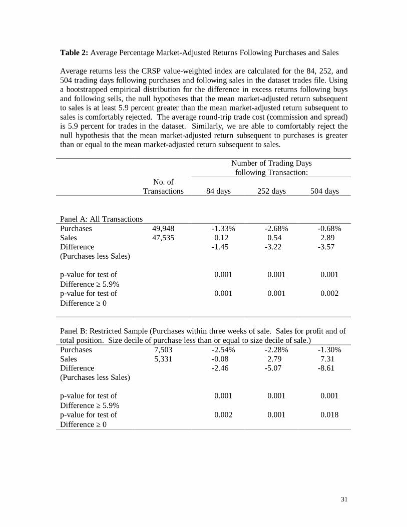
Table 2: Average Percentage Market-Adjusted Returns Following Purchases and Sales
Average returns less the CRSP value-weighted index are calculated for the 84, 252, and504 trading days following purchases and following sales in the dataset trades file. Usinga bootstrapped empirical distribution for the difference in excess returns following buysand following sells, the null hypotheses that the mean market-adjusted return subsequentto sales is at least 5.9 percent greater than the mean market-adjusted return subsequent tosales is comfortably rejected. The average round-trip trade cost (commission and spread)is 5.9 percent for trades in the dataset. Similarly, we are able to comfortably reject thenull hypothesis that the mean market-adjusted return subsequent to purchases is greaterthan or equal to the mean market-adjusted return subsequent to sales.
Number of Trading Daysfollowing Transaction:
No. ofTransactions 84 days 252 days 504 days
Panel A: All TransactionsPurchases 49,948 -1.33% -2.68% -0.68%Sales 47,535 0.12 0.54 2.89Difference(Purchases less Sales)
-1.45 -3.22 -3.57
p-value for test ofDifference ≥ 5.9%
0.001 0.001 0.001
p-value for test ofDifference ≥ 0
0.001 0.001 0.002
Panel B: Restricted Sample (Purchases within three weeks of sale. Sales for profit and oftotal position. Size decile of purchase less than or equal to size decile of sale.)Purchases 7,503 -2.54% -2.28% -1.30%Sales 5,331 -0.08 2.79 7.31Difference(Purchases less Sales)
-2.46 -5.07 -8.61
p-value for test ofDifference ≥ 5.9%
0.001 0.001 0.001
p-value for test ofDifference ≥ 0
0.002 0.001 0.018

32
Figure 1: Prospect Theory Value Function

33
Figure 2: Proportion of Gains Realized (PGR) and Proportion of Loses Realized (PLR)
This figure compares the aggregate Proportion of Gains Realized (PGR) to the aggregateProportion of Losses Realized (PLR), where PGR is the number of realized gains dividedby the number of realized gains plus the number of paper (unrealized) gains, and PLR isthe number of realized losses divided by the number of realized losses plus the number ofpaper (unrealized) losses. Realized gains, paper gains, losses, and paper losses areaggregated over time (1987-1993) and across all accounts in the data set. PGR and PLRare reported for the entire year, for December only, and for January through November.For the entire year there are: 13,883 realized gains, 79,658 paper gains, 11,930 realizedlosses, and 110,348 paper losses. For December there are: 866 realized gains, 7,131 papergains, 1,555 realized losses, and 10,604 paper losses. The t-statistics test the nullhypotheses that the differences in proportions are equal to zero assuming that all realizedgains, paper gains, realized losses, and paper losses result from independent decisions.
0.0980.094
0.128
0.1480.152
0.108
0.00
0.02
0.04
0.06
0.08
0.10
0.12
0.14
0.16
All Months Jan - Nov December
PGRPLR
34
Figure 3: Ratio of Proportion of Gains Realized (PGR) to the Proportion of LossesRealized (PLR) for each Month
PGR is the number of realized gains divided by the number of realized gains plus thenumber of paper (unrealized) gains, and PLR is the number of realized losses plus thenumber of (unrealized) losses. Realized gains, paper gains, losses, and paper losses areaggregated over time (1987-1993) and across all accounts in the data set.
0.0
0.5
1.0
1.5
2.0
2.5
Jan Feb Mar Apr May June Jul Aug Sept Oct Nov Dec
PG
R/P
LR
35
Figure 4: Market-Adjusted Returns subsequent to Buys less Market-Adjusted Returnssubsequent to Sells
Market-adjusted returns are security returns less the CRSP value-weightedNYSE/ASE/Nasdaq index. Day 0 is the day of a buy or sell. The graph depicts themarket-adjusted returns subsequent to buys less the market-adjusted returns subsequent tosells. There are 49,948 buys and 47,535 sells.
-4.00
-3.50
-3.00
-2.50
-2.00
-1.50
-1.00
-0.50
0.001 51 101 151 201 251 301 351 401 451 501
Trading Days After Purchase or Sale
Per
cent
age
Mar
ket-
Adj
uste
d R
etur
ns