Munich Personal RePEc Archive Globalization misguided views OBREGON, CARLOS 9 April 2018 Online at https://mpra.ub.uni-muenchen.de/85813/ MPRA Paper No. 85813, posted 13 Apr 2018 03:34 UTC

Welcome message from author
This document is posted to help you gain knowledge. Please leave a comment to let me know what you think about it! Share it to your friends and learn new things together.
Transcript
Munich Personal RePEc Archive
Globalization misguided views
OBREGON, CARLOS
9 April 2018
Online at https://mpra.ub.uni-muenchen.de/85813/
MPRA Paper No. 85813, posted 13 Apr 2018 03:34 UTC
GLOBALIZATIONMisguided Views
by
CARLOS OBREGÓN
[5]
INDEX
introduction 7
the ict revolution and economic development 18
nationalism and changes in
the income distribution 86
a new look at the 2008 crisis 165
the ict revolution and
the international economic order 225
policy alternatives for developed
and developing countries 265
annex 295
bibliography 302
[7]
INTRODUCTION
Science is about finding the fundamental causes of social events. Today, the world is in an evident disarray; many things seem to have gone wrong at once. Various topics: terrorism, drug trafficking, money laundering, black accounts; financial crises, income distribution, global coordination; or the social angriness and growing anti-migration —nationalistic-protec-tionist— sentiments and policies, show that something has changed for the worse. As we will see, all these events have a common deep cause that we must first understand, in order to be able to cope with its con-sequences. We are living a technological revolution that, in many ways, surpasses the so-called Industrial Revolutions, particularly because of the speed at which it is bringing change.
In these pages, we defend that institutions have not yet adapted to the new world that this technological revolution has brought about. Today’s inadequate institutional arrangements are sustained by old concepts or economic theories and ideas that no longer work as they did before. This mismatch between the new technological world and the old institutions explains most of today’s world economic problems, such as:
1. The 2008 financial crisis —its fast dissemination in the devel-oped world and the slow recovery we are facing.
2. The booms in the real estate and stock markets.3. The low level of inflation and the decline in long-term interest
rates.4. The spread of nationalism and protectionism in developed
countries —that brought, consequently, Brexit and Donald Trump winning in the USA elections.
5. The success of anti-migration policies.6. The fast growth of China —a dictatorial communist country
that did not follow the recommendations of the international governance economic institutions— and the nil growth of Mexico that did follow such recommendations.
7 The deterioration in the income distribution in many countries and the improvement in the global income distribution.
8 Japan’s economic stagnation.
carlos obregón8
9 The growing amounts in money laundering and black ac-counts.
10 The increase in criminal activities like weapons, human and drug trafficking.
11 The increase in terrorism.As Thorstein Veblen taught us, a social institution consists of both: a
conceptual system and the actual institutional arrangement, which instru-ments the social concepts1. Institutions change at the technological level (like in Veblen’s and Marx’ thought) as well as at the social and con-ceptual levels. Ideas and social engineering are relevant for institutional dynamics as Nobel price Douglas North has shown2.
The thesis presented here is that our global ideas and social engi-neering have been unable to adapt with the speed that the Information and Communications Technology (ICT) revolution, we are living, demands. Computing and data storage costs have decreased astronomically —the I. Transmission advances have improved communication beyond be-lief— the C. Likewise, the technology of new work place organizations and working methods have changed dramatically —the T. However, our ideas and our social engineering lagged behind. Ideas are important be-cause they guide the future changes of our social institutional arrange-ments. Today’s ideas relate to informational sets belonging to the past and, as consequence, we have an erroneous image of the world3 (as Kenneth Boulding wrote in The Image). In normal times, the process that coordinates new technology, new social concepts —or ideas— and new institutional arrangements is somewhat smooth, but when rapid changes happen, the process can be very disruptive as it occurs today.
The ICT revolution has made possible to manage corporations at a distance for a very low cost. The consequence has been that international firms have fragmented their manufacturing production in several coun-tries searching for the competitive advantage that low wages represent in developing countries (explaining why China has grown so fast). The ICT revolution made it possible to diffuse knowledge internationally —and it generates growth as Romer’s model clearly shows4. China’s fast growth is the main reason (although other countries start to be relevant also)
1 Thorstein Veblen, 1914.
2 Douglas North, 2005.
3 Kenneth E Boulding, 1971.
4 For an overview on economic growth models, see Obregon 2008a, chapter 5.
introduction 9
that, for the first time, the global income distribution is improving. So the winners and the losers of the new wage technology explain, as Branko Milanovic 2016 brilliantly shows, the income distribution deterioration in many countries. The winners are those that benefit from the new produc-tion mode: on one side the elite in the developed world —or the owners of the international firms—, on the other side, China’s and other developing countries’ population that benefited from their new participation in the global process of production. The losers are the workers in the developed countries previously employed in the manufacturing sector.
Since firms are already using low-wage workers in the developing countries, by fragmenting manufacturing processes, they no longer have the need to obtain low-paid manual labor at home through migration. The consequence is that firms decreased their pro-migration lobbying at the same time that the affected middle class in the developed world has become more willing to hear and support the anti-migration propaganda of radical right movements. This is the explanation for the success of anti-migration policies in several developed countries around the world5.
The world has become integrated not only in manufacturing but also in finances. The new ICT facilitated the interconnection of the global banking system. Global financing developments were a natural companion of the new ICT boom. This globalization explains why, what was considered only a local American problem in a very particular market —the subprime real estate, became a global crisis dimensionaly similar to The Great Depression of the 1930s. At the end, this crisis was fortunately somewhat contained because the institutions are now better designed, compared to those in the 30s. Policy makers in today’s institutions had the advantage of both the experience of the 30s and the recent Japanese’s deflation. The question is why a supposed local phenomenon created such a big international financial crisis. The an-swer, as it will be shown, is that our ideas —our economic theory and our institutional arrangement— were initially unable to cope with the full-blown implications of an unprecedented revolution that globalized finances, related to the unbelievable fast ICT changes. This unprec-edented global revolution in finances happened at the beginning of a crisis poorly understood by the regulators.
Policy makers have been caught by surprise by two recent trends: a) inflation remains subdued despite economic recovery, b) the recovery has been very slow in the USA and is not quite yet happening in Europe.
5 Margaret Peters (2017) have presented a convincing empirical verification of this argument.
carlos obregón10
Consequently, the policy rate has remained unusually low. Mervyn King (governor of the Bank of England from 2003 to 2013) authoritatively argues that we have been applying, and still are, the wrong economic theory to understand the recent phenomena6. The new mode of produc-tion implies large productivity increases due to the massive introduction of low-wage workers and that is what maintains inflation subdued. In addition, the recovery has been very slow because consumers and inves-tors lost confidence in the future —what King, based upon Frank Knight and John Maynard Keynes, calls radical uncertainty— and it is returning very slowly.
China’s participation in the global economy (along with other Asian countries, to a lesser extent) have produced both: an increase in global productivity that has maintained inflation subdued in the developed world through cheap imports —which has lowered long-term inflationary expecta-tions and, therefore, the long-term nominal rate— and an increase in global savings —which reduced the long-term real rate of interest. This dual phe-nomenon promoted the demand for long duration assets, such as the real estate and stock markets, which explains their boom. In addition:
1. Expected profit increases due to the ICT revolution have stim-ulated furthermore the demand for stocks and the increase in its price.
2. While firms exported and fragmented their global manufactur-ing production, they maintained at home manufacturing ser-vices —that is, tasks before and after production such as plan-ning and marketing, as well as coordinating tasks.
Manufacturing services benefits from economies of scale related to hubs of high skilled professionals, concentrated in urban areas. The boom in manufacturing services as well as the one in the financial sec-tor —that concentrates in the cities as well— meant an additional demand pressure that increased even more the real estate prices in urban areas.
A very strange interpretation of economic theory is found in the official explanation of the 2008 financial crisis. It argues that the crisis was due to the so-called savings glut, which reduced real ex-ante long-term interest rates and fostered the real estate boom fueled by irrationality. The boom eventually had to crash and this explains the crisis. This, of course, is an ex-post explanation, a very curious one because, with free exchange rates, autonomous Central Banks did not have to accept the extra savings arriving to their economies, a point that King explicitly
6 Mervyn King, 2016.

introduction 11
recognizes –although argues that it would have been a herculean task for an isolated central bank–. Although we agree with him, we believe the Federal Reserve could have certainly done it, but decided not to. Beyond this technicality, what is critical to understand is that the argument where trade unbalances —which caused the saving glut— produced the crisis is incorrect. What people were expecting ex-ante according to theory was a weaker dollar —which did not happen, nor a real estate crisis. In fact, the crisis started in the USA, one of the countries where the real estate boom had been less strong.
We will demonstrate that the crisis started not as a generalized real estate crash but as a subprime crash of adjustable rate loans caused by the Fed’s interest rate going down to 1% at first, then up to 6% in just few years. Now, because the subprime loans had been safeguarded in com-plex securities, distributed all over the world with 2/3 of the private sector holdings in banks, these could not estimate what was the actual impact of the subprime crisis in a given particular bank. As a result, the banking crisis starts. It first appears with the rise of the interbank lending rate, the Libor, then in bank’s lending rates to the public. This rise in interest rates is what produces the generalized real estate crash, later on.
The order of events is crucial to understand the crisis; it shows that the regulators had opportunities to intervene and prevent the crisis from spreading. It would have been very inexpensive —compared to the actual costs we have had— to take out the subprime loan paper from the market. Then, the question is: why was it not done?
We will argue this: that the financial crisis in 2008 did not have to happen, it was the consequence of old ideas —economic theories— that institutions applied to a new reality, one they could not explain or con-trol. The old theory told us that risk could be managed. Several Nobel prices were given to celebrate this achievement. Regulators expected the market itself to be able to succeed –because risk is probabilistic. For three consecutive years, the Economic Report of the President claimed that the subprime crisis was going to be managed efficiently by the mar-ket. Meanwhile, the Federal Reserve stood away from the problem de-spite its mandate to regulate financial institutions. At the same time, the Europeans maintained that this was a particular problem of the USA economy not related to them. Had the treasury and the Fed intervened in early stages, the subprime crisis would have been controlled and we would have not had the 2008 international financial crisis. However, they did not do it because they were convinced that the markets were
carlos obregón12
going to stabilize the problem. They never understood that uncertainty —in the sense of Knight or Keynes’— cannot be managed by the mar-ket. Regulators are responsible of maintaining an adequate institutional framework, capable to provide the certainty required. Regulators have to closely follow the financial developments and understand their pos-sible consequences. They have gotten away from the markets under the belief that these were going to manage risks much better than the government’s agencies. They were wrong. Due to their distance from the markets, the regulators never understood that, in the context of the increasingly rapid sophistication and internalization of global finances, the adjustable loans subprime crash was a potential economic bomb that could produce drastic global consequences.
The old neoclassical theory taught us that reducing trade barriers, re-ducing the government size, balancing budgets and letting prices adjust freely would attract the required amounts of foreign investment, therefore, developing economies would grow. The proposal was theoretically sound. To maximize global production, the factors of production were supposed to be allocated according to their competitive advantage —therefore, capital was supposed to flow to those countries with low wage levels. Neverthe-less, it did not work in practice for the reasons that developing economies have different institutional arrangements than the developed ones. This translates into additional costs and risks for all sort of reasons: infrastruc-ture, bureaucratic and untrustworthy administrative procedures, and a fundamental mistrust as to the long-term stability of the local legal frame due to political risks. This meant that the required extra-compensation, due to the additional risk, outweighed in many cases the benefits of the low wage. Particularly, transferring long-term investment capital means trans-ferring proprietary technology —a huge risk for multinationals that do not consider the local legal frame solid enough. Thus, long-term capital flows were not as high as expected; many investors chose the route of short-term financial investments, which at the end was one of the reasons of the well-known financial crises in the developing economies.
While the neoclassical model failed, the Asian Development Model applied by Japan and others was successful. This model was based on:
a) Huge local savings, which were the ones that financed long-term growth.
b) A trade surplus that gave them control and stability on their exchange rate through increased Central Bank reserves, avoid-ing the fluctuations produced by short term capital flows.
introduction 13
c) A flexible industrial plan based in transferring knowledge from foreign companies, giving them in exchange good conditions for their investments.
The ICT revolution changed the panorama. It made it possible for firms to export their manufacturing process fragmented and to provide centrally manufacturing services that reduce their risk of transferring confidential proprietary knowledge. Multinationals were willing to go to any country that offered them, basically, three guarantees:
1. Free movement of investments in and out of the country.2. Ensuring global class services such as telecoms, shipping and
custom clearance.3. Intellectual property protection. With the failure of the neoclassical model, some developing countries
decided to offer better conditions to the firms by satisfying as far as pos-sible the three mentioned requirements.
Since manufacturing services remained home, an important consider-ation was the still high cost of personally visiting the offshore locations. Asia was well positioned, it had a large labor supply located in a few countries (mostly in China) and wages were extremely low. The firms went to China and to a lesser extent to Mexico (which only received in-vestments due to NAFTA). China made much better offers to firms than Mexico. It had mercantilist policies that prevented huge imports and, when it joined the World Trade Organization (WTO), it devalued its currency to protect its local industry7. China had also had a dual wage: lower for Chinese companies that hired illegal immigrants (that is, labor going illegally from one Chinese state to the other) and higher for foreign companies that had to hire legal workers. Mexico played by the rules. Its imports were high due to the lack of mercantilist policies, exchange rate was truly free and there was only one wage rate. China had high savings that financed a rapidly increasing local investment, one that fostered a fast economic growth and allowed growing local firms to learn quicker from foreign companies’ technology. Mexico’s savings were low and it sticked to the old neoclassical views of free trade and free exchange rate; therefore, it did not develop its own industrial policy. The consequences were an unstable exchange rate, a much slower learning of the foreign technology, higher imports and nil economic growth.
The comparison between China and Mexico makes it clear that the old neoclassical ideas were wrong. Mexico sticked to them and, despite
7 China joined the WTO on December 11, 2001.
carlos obregón14
its intense participation in the ICT revolution due to the NAFTA, it did not grow. What the theory did not understand was that it was no longer a question of countries’ competition —general trade barriers amongst coun-tries were no longer the issue. International trade theory is based upon national competitiveness (competitive advantage that no longer works with firms fragmented in several countries). That is why the Washington Consensus did not work. What really counts is how well do countries provide the role of host for international firms, for specific fragmented processes of production, and not the overall country’s economic competi-tiveness —or the quality of its overall economic policies— measured by neoclassical standards.
Fragmented plants of a firm’s manufacturing was the relevant factor in the ICT revolution. China understood this, gave the firms superior conditions and succeeded against theoretical expectations. A key factor in China’s success story was to have applied the Asian Development Model instead of the old neoclassical model. What this experience revealed is that the marginal countries capable to develop new institutions and adapt to the new technological requirements, are the ones that succeed. No doubt NAFTA helped Mexico, without it, it would have grown even less and with less quality8. However, the NAFTA is founded with old ideas that did not help Mexico exploit efficiently the new conditions provided by the ICT revolution. China by using the Asian Development Model has been, by far, the main beneficiary of the mentioned revolution.
Given the degree of trade openness in the world, some authors have argued that the next big productivity increase could come from migra-tion9. Then again, this recommendation misses the point that firms, for the most part, do no longer need migration. The productivity increase these authors were looking for is already happening because of the frag-mented manufacturing process, which uses the low wage labor in devel-oping economies. This solution offers the firms even cheaper labor than migration because wages are local, subject to its local laws and social norms of the developing country. Wages and norms that in most cases would have become unacceptable in the developed world; therefore, mi-gration in practice means increasing the wage cost. In a sense, the ICT
8 By less quality we mean growth based upon obsolete technologies, in which industries lose value quickly when exposed to foreign imports competition from global competitive markets with frontier technology, as it happened with East Germany when it joined West Germany.
9 See Rodrik (2011) for example.

introduction 15
revolution can be thought as reverse migration: instead of labor going to developed countries, fragmented technology goes to the developing ones.
Neoclassical economic theory also claimed that openness and an ad-equate macroeconomic behavior including free exchange rates would prevent financial crises. The reality is that capital flows can be very spec-ulative, to the point that in the Asian crisis, at the end of the 90s, the financial contagion reached countries that —according to theory— had very sound macro and micro economic fundamentals. In fact, countries with exchange controls, like Malaysia and China, were the ones that did better in the crisis. The theoretical insistence in avoiding the moral haz-ard made the International Monetary Fund (IMF) programs insufficient and inadequate. In order to avoid both the large costs associated with future financial crisis and the significant costs paid by countries as a result of establishing exchange controls, the Asian economies and others —like Mexico most recently— decided to substantially increase their level of international reserves. This increased global savings even further.
The 2008 financial crisis was costly for the middle class in developed economies. This has produced a return in nationalism and protectionism, which goes hand in hand with the actual recommendations for balancing global trade made by several international institutions. Such recommen-dations are based on traditional international trade theory and advice balancing trade among countries to avoid a future potential financial cri-sis due to creditors’ untrusting debtors10. But traditional trade theory is the wrong frame to understand the ICT revolution. Take for example USA and China; they are so tight together that China cannot seriously untrust a payment from the counter part. Moreover, the USA can always pay by printing USA dollars; let us suppose China sells USA’s bonds, the USA Fed could buy bonds from the market from the same amount with printed money and this is the end of the story. Of course, the real-ity is that it would create serious financial speculation and private sector concerns that would have to be avoided (although the whole situation is very speculative in any case). However, it would just not happen since China and USA are tied together by the ICT production mode, and that seems to be the best situation for both of them.
The recommendation of balancing trade is based on the assumption that the saving glut produced the 2008 crisis. It did not. This is why under-standing what produced the 2008 financial crisis is so fundamental. The recommendation is very risky because it goes against the ICT revolu-
10 IMF report —specifically Olivier Blanchard´s argument in the Sept, 2011 WEO.
carlos obregón16
tion. China will not substantially consume more USA products in the near future, simply because it is at a much different income level. Eighty percent of the Chinese population is poorer than USA’s second poorest income decile. They do not consume the products that the USA produces mostly due to their low income. Then, balancing trade would really mean less global trade; this means less productivity and less global growth in the future, more expected inflation and higher real interest rates, less bor-rowing capacity for the middle class in the USA and a reduction of living standards. It would not make sense to pay this huge price to prevent a risk that did not materialize in the past —as argued— and does not seem to be a risk for the future. Whatever we do, the goal of the global trade and financial system should be to allow the ICT revolution to provide humanity with the productivity increases of which it is capable.
As a final note, the reader is reminded that, even though this is not the topic of analysis of this book, fragmentation of the production process not only occurs in multinationals. Criminals also use the ICT revolution to globalize their operations, to fragment them and to make them more difficult to find. Drugs, weapons and human trafficking have become global as never before. Terrorist groups are now acquiring new members and training them through the internet. The fiscal paradises have grown more than ever —as they provide a solution not only for money escaping its fiscal obligations, but also for money laundering and all sorts of illicit money transfers. Nationalism and protectionism will make very difficult to achieve a global coordination to eliminate the fiscal paradises. And as long as they exist it will be difficult to fight efficiently against global crimi-nality and terrorism. In fact, the scarce global coordination that exists has recently been under pressure, as the announced exit of the USA from the Paris agreement shows, and as the United States pressure on the OTAN members to contribute more with military expenditures also indicates.
Fast globalization, due to the ICT revolution requires an adequate response from global leaders; its institutional arrangements must be re-newed and strengthened. The ICT revolution will bring us even closer to each other and any intent to prevent this will fail. Institutions need to adapt to the ICT revolution or the world will enter difficult times.
In the first chapter, we present the ICT economic revolution and pro-vide a historical perspective to discuss how it distinguishes itself from pre-vious ones. We use it as a frame to discuss a general theory of economic development. We review China’s recent growth and show the direction, levels and characteristics of recent trade flows. In the second chapter,
introduction 17
we discuss the income distribution at both country and global level, and how it relates to the ICT revolution. We show that the reduction in global inequality is mainly due to China, although other countries are becoming also relevant. As far as within country inequality is concerned, we show that Piketty’s 2014 book proposal regarding laws of capitalism that necessarily concentrate the income distribution is wrong. The wealth concentration that Piketty has empirically observed is due to real estate and stock market booms, which are medium-term waves better explained by the ICT revolution. This is more in tune with both Milanovic and Williamson’s recent works on global and USA income distribution. In the third chapter we review the causes of the 2008 crisis that could have been avoided and where do we stand now; how regulators left the man-agement of risk in private hands, without understanding that they were responsible for establishing institutional certainty in Knight or Keynes’ sense. In the fourth chapter we present a theoretical analysis of the global institutional arrangement in trade and finances and how it relates to the ICT revolution; we also make policy recommendations. Finally, in the fifth and final chapter we analyze policy alternatives both for developed and developing countries in the framework of the new technological rev-olution.
[18]
THE ICT REVOLUTION AND
ECONOMIC DEVELOPMENT
the ict revolution
The ICT revolution started somewhere in the mid 80s. We will use as a reference point 1990. The I stands for information, the C for commu-nications, and the T for technology particularly related to new working methods and work place organizations. In his recent and extraordinary book, Richard Baldwin notes: “Between 1986 and 2007, world informa-tion grew at 23%, per year, telecommunications at 28% and computa-tion power at 58% per year”11. To understand what it means, we must recall that global GDP per capita only grew at annual rate of 2.1%12. This means that, while GDP per capita multiplies itself 1.6 times in these twenty-one years, information multiplies by 77.3 times, telecommunica-tions by 178.4 times, and computation by 14852.5 times.
11 Baldwin 2016
12 Maddison Project 2013. In order to compare different countries along the years, one necessarily has to make adjustments. In a given year countries’comparisons have to be made using a common currency, normally being the USA dollar. To translate the values of a given country from its currency to dollars, one cannot just use the prevalent exchange rate for the simple reason that the price of a given product or service is not the same in different countries. Therefore, one needs to calculate what is known as Purchase Power Parity (PPP) dollars. These tells us that one dollar of this kind buys the same at all coun-tries and, to avoid distorsions for inflation, one uses constant dollars. Maddison is the only long historical data series calculted in PPP constant dollars. In its case, 1990 Geary-Khamis dollars. The World Bank has also calculated PPP series, the first one was in 2005 constant PPP international dollars and last one in 2011 PPP constant international dollars. The Pen Tables PPP’s are like the World Bank’s. For 2011 constant PPP international dollars, the World Bank presents data from 1990 onwards. In this work, we will use World Bank data for 1990 onwards and Maddison for any date before, unless stated otherwise. For Mad-dison, there are two series: first is the 2009 series, which is the original of Angus Maddison and presents GDP, population and GDP per capita; second one is a revised version made by his colleages, after his passed away in 2013; this series only presents GDP per capita. We will use the second series whenever we use only GDP per capita.
the ict revolution and economic development 19
Gordon Moore established what is called the Moore’s law, which states that computer power grows exponentially; George Gilder observed that bandwidth grows three times as fast as computer power; and Robert Metcalfe noted that the usefulness of a network increases with the square of the number of users. Therefore, the ICT constitutes a real revolution. The consequences of the ICT revolution have not passed unnoticed by economists. Blinder (2006) called it the next industrial revolution; Jones (1997), challenged the principle of competitive advantage; Grossman and Rossi-Hansberg (2006) pointed out the growing tradability of parts and components, and developed their notion of Trading Tasks; and Baldwin (2016) has discussed it as the second unbundling, referring to the Steam Revolution as the first unbundling. However, despite the awareness of some economists, traditional policies and dominant economic thinking have not yet adapted to the new reality, and as we will maintain, this widely explains the inadequate institutional response to the new abrupt reality brought by the ICT revolution.
The consequences of the ICT revolution are well known to all of us: internet, our mobile phone, Facebook, Twitter, Amazon, Uber and so on have changed our daily lives. What is lesser known is the extent to which it has changed the whole world economy. Whether one looks at inflation, economic growth, the global income distribution, the income distribution within countries, or almost any other economic variable, everything has changed with the ICT revolution.
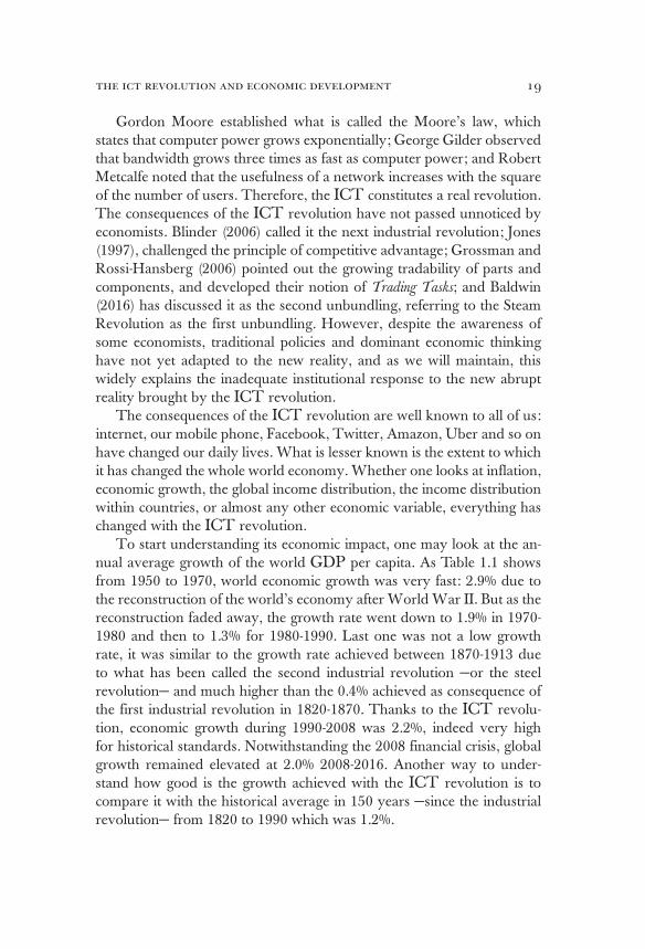
To start understanding its economic impact, one may look at the an-nual average growth of the world GDP per capita. As Table 1.1 shows from 1950 to 1970, world economic growth was very fast: 2.9% due to the reconstruction of the world’s economy after World War II. But as the reconstruction faded away, the growth rate went down to 1.9% in 1970-1980 and then to 1.3% for 1980-1990. Last one was not a low growth rate, it was similar to the growth rate achieved between 1870-1913 due to what has been called the second industrial revolution —or the steel revolution— and much higher than the 0.4% achieved as consequence of the first industrial revolution in 1820-1870. Thanks to the ICT revolu-tion, economic growth during 1990-2008 was 2.2%, indeed very high for historical standards. Notwithstanding the 2008 financial crisis, global growth remained elevated at 2.0% 2008-2016. Another way to under-stand how good is the growth achieved with the ICT revolution is to compare it with the historical average in 150 years —since the industrial revolution— from 1820 to 1990 which was 1.2%.
carlos obregón20
table 1.1. gdp world average annual growth percentage
Period 1 Maddison Project 2013 2 World Bank
1-1500 0.013*
1500-1820 0.051*
1820-1870 0.435
1870-1913 1.303
1913-1950 0.841
1950-1970 2.898
1970-1980 1.931
1980-1990 1.333
1990-2008 2.205 2.063
2008-2016 NA 1.957
Source: 1] The Maddison-Project, http://www.ggdc.net/maddison/maddison-project/home.htm, 2013 version; periods 1-1500 and 1500-1820 (*) come from Angus Maddison 2009, original base available at same site. 2] The World Bank: http://databank.worldbank.org, last updated 08/02/2017.
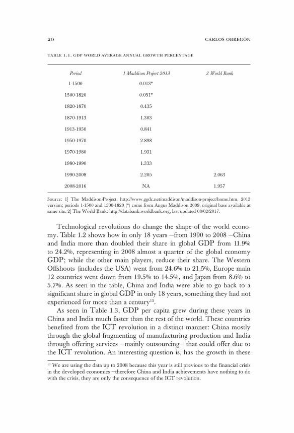
Technological revolutions do change the shape of the world econo-my. Table 1.2 shows how in only 18 years —from 1990 to 2008 —China and India more than doubled their share in global GDP from 11.9% to 24.2%, representing in 2008 almost a quarter of the global economy GDP; while the other main players, reduce their share. The Western Offshoots (includes the USA) went from 24.6% to 21.5%, Europe main 12 countries went down from 19.5% to 14.5%, and Japan from 8.6% to 5.7%. As seen in the table, China and India were able to go back to a significant share in global GDP in only 18 years, something they had not experienced for more than a century13.
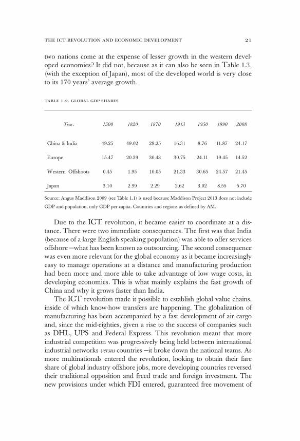
As seen in Table 1.3, GDP per capita grew during these years in China and India much faster than the rest of the world. These countries benefited from the ICT revolution in a distinct manner: China mostly through the global fragmenting of manufacturing production and India through offering services —mainly outsourcing— that could offer due to the ICT revolution. An interesting question is, has the growth in these
13 We are using the data up to 2008 because this year is still previous to the financial crisis in the developed economies —therefore China and India achievements have nothing to do with the crisis, they are only the consequence of the ICT revolution.
the ict revolution and economic development 21
two nations come at the expense of lesser growth in the western devel-oped economies? It did not, because as it can also be seen in Table 1.3, (with the exception of Japan), most of the developed world is very close to its 170 years’ average growth.
table 1.2. global gdp shares
Year: 1500 1820 1870 1913 1950 1990 2008
China & India 49.25 49.02 29.25 16.31 8.76 11.87 24.17
Europe 15.47 20.39 30.43 30.75 24.11 19.45 14.52
Western Offshoots 0.45 1.95 10.05 21.33 30.65 24.57 21.45
Japan 3.10 2.99 2.29 2.62 3.02 8.55 5.70
Source: Angus Maddison 2009 (see Table 1.1) is used because Maddison Project 2013 does not include
GDP and population, only GDP per capita. Countries and regions as defined by AM.
Due to the ICT revolution, it became easier to coordinate at a dis-tance. There were two immediate consequences. The first was that India (because of a large English speaking population) was able to offer services offshore —what has been known as outsourcing. The second consequence was even more relevant for the global economy as it became increasingly easy to manage operations at a distance and manufacturing production had been more and more able to take advantage of low wage costs, in developing economies. This is what mainly explains the fast growth of China and why it grows faster than India.
The ICT revolution made it possible to establish global value chains, inside of which know-how transfers are happening. The globalization of manufacturing has been accompanied by a fast development of air cargo and, since the mid-eighties, given a rise to the success of companies such as DHL, UPS and Federal Express. This revolution meant that more industrial competition was progressively being held between international industrial networks versus countries —it broke down the national teams. As more multinationals entered the revolution, looking to obtain their fare share of global industry offshore jobs, more developing countries reversed their traditional opposition and freed trade and foreign investment. The new provisions under which FDI entered, guaranteed free movement of
carlos obregón22
capital, access to world-class services, and intellectual property protection. Fragmented production meant that competition was no longer country sector based; developing nations became part of the competition stage by stage. This accelerated productivity a lot.
table 1.3. gdp per capita annual growth rates percentage
Period: 1500-1820 1820-1990 1990-2008
China 0.00 0.67 7.37
India 0.00 0.53* 4.62
Japan 0.10 1.98* 0.92
Europe 121 0.14 1.42 1.60
Western Offshoots 0.34 1.69 1.69
USA 0.36 1.68 1.67
Source according to period: Angus Maddison 2009 (1500-1820); Maddison Project 2013 (1820-1990 and 1990-2008), except India and Japan (*) also from Angus Maddison 2009.
1 Twelve main countries. From this point on we represent with a figure, next to the name of region, the number of countries considered in that particular data.
The ICT revolution implied that new economic zones with new rules, belonging to a selected group of developing economies, became all of a sudden an important part of the regular complex trade that had been tak-ing place amongst developed economies, involving not only goods and services, but investments, skilled people, and know-how. The new rules established in the new value chains made the process as trustable as if it was happening within the confines of the developed world.
Fragmenting production made it possible to disaggregate manufac-turing services from manufacturing production. Activities like planning, product design, general management, general coordination of manufac-turing production, financial decisions, and marketing strategies are now performed in the developed economies multinational’s urban offices un-der the general heading of manufacturing services, while manufactur-ing production itself happens fragmented offshore in a selected group of developing countries. This is the case of Apple, whose manufacturing

the ict revolution and economic development 23
services take place in California while actual production occurs in China, organized by unrelated companies.
Historically, industrial activity was concentrated in developed coun-tries, due to the scale economies of industrial activities together, and they had high costs of migration due to all sort of institutional barriers en-countered in the developing countries. Besides its advantages, though, this process meant producing with high wages. The ICT revolution made it possible to maintain the economies of scale in manufacturing services —planning, general managing, marketing, and so on— while en-joying the low wages of the developing economies. It made it possible to fragment the manufacturing process while still manage them efficiently from the urban centers in the developed economies. However, there were still important scale economies associated with having the manufacturing processes somewhat together; therefore, one can speak of industrial con-glomerates by region like Asia, Europe, and North America. Being the first the most successful one.
Growth of China and India meant that a large portion of the world population could increase its income and this generated commodities de-mand that brought growth to the commodities exporting producing coun-tries that were not originally part of the ICT industrial revolution. This revolution, as expected, has had winners and losers, as well as its relevant consequences for the global income distribution. The winners were:
a) Large technological firms based in developed nations, which have had unusually high returns14, the consequence: a stock market boom.
b) High skill workers in developed nations due to the higher de-mand for financial and manufacturing services.
c) The owners of real estate; the boom of financial and manu-facturing services concentrated in urban centers in developed economies, and produced a real estate boom in these areas. Since ownership of real estate and stock market is concentrated in rich people, the rich became richer.
d) Low paid workers in the selected group of developing nations that joined the ICT revolution, who have become more productive.
e) Those countries that benefited from the commodities boom associated with the higher global demand consequence of the higher global growth and the new demand of the fast-growing Asian giants.
14 See Hall 2016
carlos obregón24
f) The general population of the world —but particularly of the developed countries— which enjoyed the higher global produc-tivity as reflected in lower prices, lower expected inflation, and lower long-term interest rates, both real and nominal.
The losers were: a) Low skill workers in manufacturing production processes in devel-
oped economies; which not only were seeing their jobs disap-pear, but also their traditional bargaining power —as the same process that held them together started to vanish.
b) Developed nations that did not join efficiently the ICT revolution, like Japan.
c) Developing nations that did not join it.Developing nations that joined the ICT revolution with old unsuitable
ideas, like Mexico, had both winners and losers. The winners were the firms and workers associated with the ICT revolution, the losers, the rest of the economy which suffered from low growth given the country’s in-ability to use the ICT revolution to foster local national economic growth. The income distribution consequences will be the topic of the next chapter.
The referred revolution produced in the developed economies a polar-ization of the work force. At the top end, highly skilled workers are doing better than ever. At the low-end, low-skilled workers are doing fine because of economic growth related to the increase in global productivity. In the middle low skill, manufacturing workers are losing their jobs due to that revolution, through two distinct channels: their jobs have been moving offshore to selected developing economies and the revolution meant an acceleration of automated process. This automation is only beginning; it certainly will become the way of the future. The unexpected 2008 financial crisis made the polarization much worse. With no economic growth, not only the relative income of the low-skill workers in manufacturing was worse but also their actual absolute income went down. Even the ones in the service sector lost the benefits related to economic growth. Unemploy-ment shot up high and the worker’s value assets in general went down.
As we will see in the third chapter, the 2008 financial crisis goes a long way to explain the growing nationalistic and protectionist sentiments that produced the votes for Brexit and Mr. Trump. The deterioration of the income distribution due to the so-called revolution had already occurred before the crisis started and had not produced the nationalistic and protec-tionist sentiments observed after the crisis. But to fully explain this point, we will need to wait for the explanations provided in the third chapter.
the ict revolution and economic development 25
As far as governments in the developed world is concerned, the ICT revolution is company base, so there is very little they can do to promote or to stop it. In the case of the developing economies, governments do have a role to play: they mostly promote the adequate conditions to become a competitive recipient of the foreign direct investment of the large global firms. Any attempt by a developed economy to go against the ICT revolution will have drastic, undesired consequences in its long-term economic growth because its technology will become uncompeti-tive. Governments in the developed economies, however, should do a much better job in creating adequate institutions capable of solving the structural and income distribution imbalances that this abrupt revolution generated. On the other side, governments in the developing nations that do not actively join the transformation are condemning their countries to old technologies that will eventually be wiped out by the new modern technologies, leaving enormous economic and social costs. This is why governments in developing economies must define an industrial plan that guarantees that the ICT revolution translates itself in national economic growth and benefits the local population. This topic will be discussed further in chapter five.
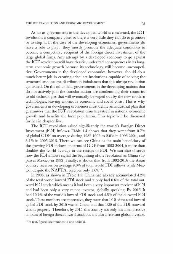
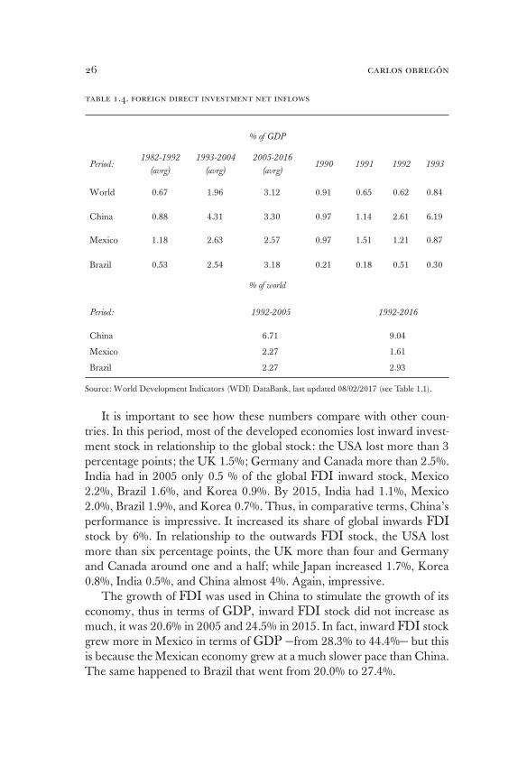
The ICT revolution raised significantly the world’s Foreign Direct Investment (FDI) inflows. Table 1.4 shows that they went from 0.7% of global GDP on average during 1982-1992 to 2.0% in 1993-2004, and 3.1% in 2005-2016. There we can see China as the main beneficiary of the growing FDI inflows; in terms of GDP from 1993-2004, it more than doubles the world average in the receipt of FDI. We can also observe how the FDI inflows signal the beginning of the revolution as China sur-passes Mexico in 1992. Finally, it shows that from 1992-2016 the Asian country receives on average 9.0% of total world FDI inflows while Mex-ico, despite the NAFTA, receives only 1.6%15.
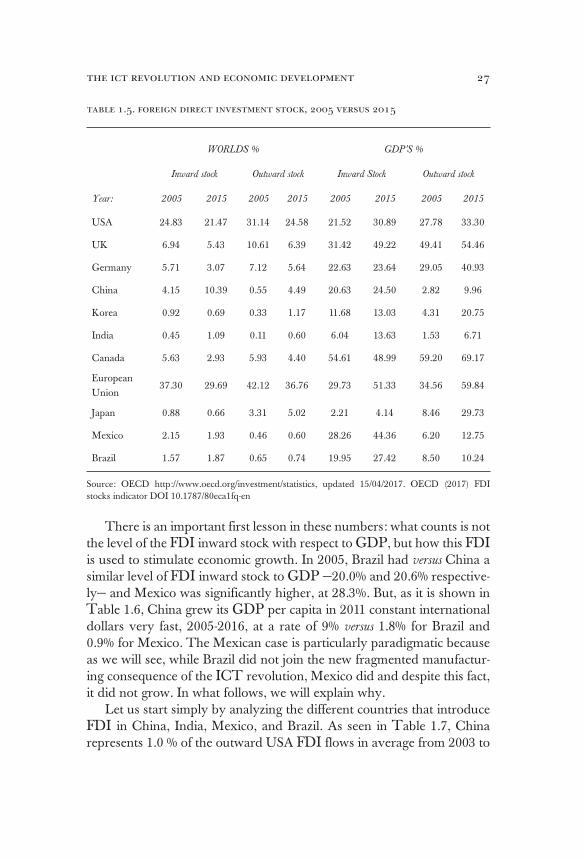
In 2005, as shown in Table 1.5, China had already accumulated 4.2% of the total world inward FDI stock and it only had 0.6% of the total out-ward FDI stock which means it had been a very important receiver of FDI and had been only a very minor investor, globally speaking. By 2015, it had 10.4% of the world’s inward FDI stock and 4.5% of the outward FDI stock. These numbers are impressive, they mean that 1/10 of the total inward global FDI stock by 2015 was in China and that 1/20 of the FDI outward was its property. Therefore, by 2015, this country not only has an impressive amount of foreign direct inward stock but it is also a relevant global investor.
15 In text, figures are rounded to one decimal.
carlos obregón26
table 1.4. foreign direct investment net inflows
% of GDP
Period:1982-1992
(avrg)
1993-2004
(avrg)
2005-2016
(avrg)1990 1991 1992 1993
World 0.67 1.96 3.12 0.91 0.65 0.62 0.84
China 0.88 4.31 3.30 0.97 1.14 2.61 6.19
Mexico 1.18 2.63 2.57 0.97 1.51 1.21 0.87
Brazil 0.53 2.54 3.18 0.21 0.18 0.51 0.30
% of world
Period: 1992-2005 1992-2016
China 6.71 9.04
Mexico 2.27 1.61
Brazil 2.27 2.93
Source: World Development Indicators (WDI) DataBank, last updated 08/02/2017 (see Table 1.1).
It is important to see how these numbers compare with other coun-tries. In this period, most of the developed economies lost inward invest-ment stock in relationship to the global stock: the USA lost more than 3 percentage points; the UK 1.5%; Germany and Canada more than 2.5%. India had in 2005 only 0.5 % of the global FDI inward stock, Mexico 2.2%, Brazil 1.6%, and Korea 0.9%. By 2015, India had 1.1%, Mexico 2.0%, Brazil 1.9%, and Korea 0.7%. Thus, in comparative terms, China’s performance is impressive. It increased its share of global inwards FDI stock by 6%. In relationship to the outwards FDI stock, the USA lost more than six percentage points, the UK more than four and Germany and Canada around one and a half; while Japan increased 1.7%, Korea 0.8%, India 0.5%, and China almost 4%. Again, impressive.
The growth of FDI was used in China to stimulate the growth of its economy, thus in terms of GDP, inward FDI stock did not increase as much, it was 20.6% in 2005 and 24.5% in 2015. In fact, inward FDI stock grew more in Mexico in terms of GDP —from 28.3% to 44.4%— but this is because the Mexican economy grew at a much slower pace than China. The same happened to Brazil that went from 20.0% to 27.4%.
the ict revolution and economic development 27
table 1.5. foreign direct investment stock, 2005 versus 2015
WORLD´S % GDP’S %
Inward stock Outward stock Inward Stock Outward stock
Year: 2005 2015 2005 2015 2005 2015 2005 2015
USA 24.83 21.47 31.14 24.58 21.52 30.89 27.78 33.30
UK 6.94 5.43 10.61 6.39 31.42 49.22 49.41 54.46
Germany 5.71 3.07 7.12 5.64 22.63 23.64 29.05 40.93
China 4.15 10.39 0.55 4.49 20.63 24.50 2.82 9.96
Korea 0.92 0.69 0.33 1.17 11.68 13.03 4.31 20.75
India 0.45 1.09 0.11 0.60 6.04 13.63 1.53 6.71
Canada 5.63 2.93 5.93 4.40 54.61 48.99 59.20 69.17
European Union
37.30 29.69 42.12 36.76 29.73 51.33 34.56 59.84
Japan 0.88 0.66 3.31 5.02 2.21 4.14 8.46 29.73
Mexico 2.15 1.93 0.46 0.60 28.26 44.36 6.20 12.75
Brazil 1.57 1.87 0.65 0.74 19.95 27.42 8.50 10.24
Source: OECD http://www.oecd.org/investment/statistics, updated 15/04/2017. OECD (2017) FDI stocks indicator DOI 10.1787/80eca1fq-en
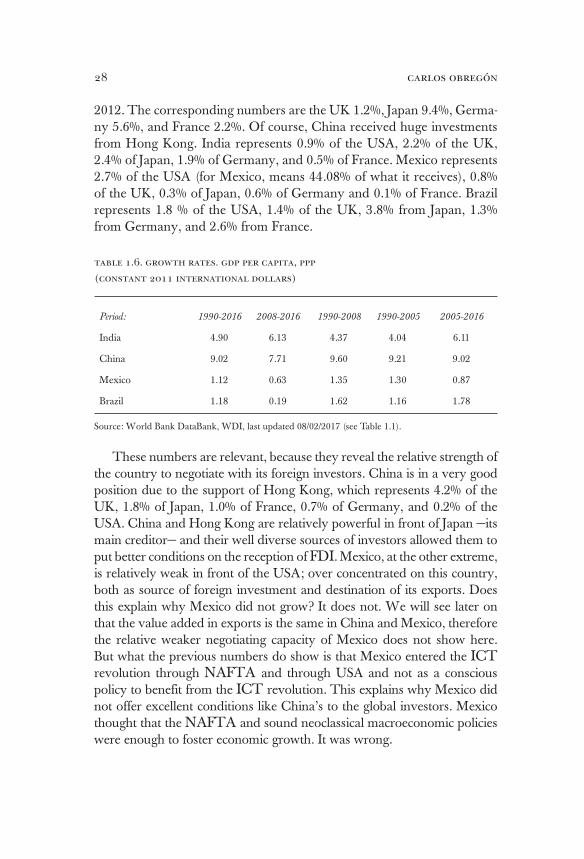
There is an important first lesson in these numbers: what counts is not the level of the FDI inward stock with respect to GDP, but how this FDI is used to stimulate economic growth. In 2005, Brazil had versus China a similar level of FDI inward stock to GDP —20.0% and 20.6% respective-ly— and Mexico was significantly higher, at 28.3%. But, as it is shown in Table 1.6, China grew its GDP per capita in 2011 constant international dollars very fast, 2005-2016, at a rate of 9% versus 1.8% for Brazil and 0.9% for Mexico. The Mexican case is particularly paradigmatic because as we will see, while Brazil did not join the new fragmented manufactur-ing consequence of the ICT revolution, Mexico did and despite this fact, it did not grow. In what follows, we will explain why.
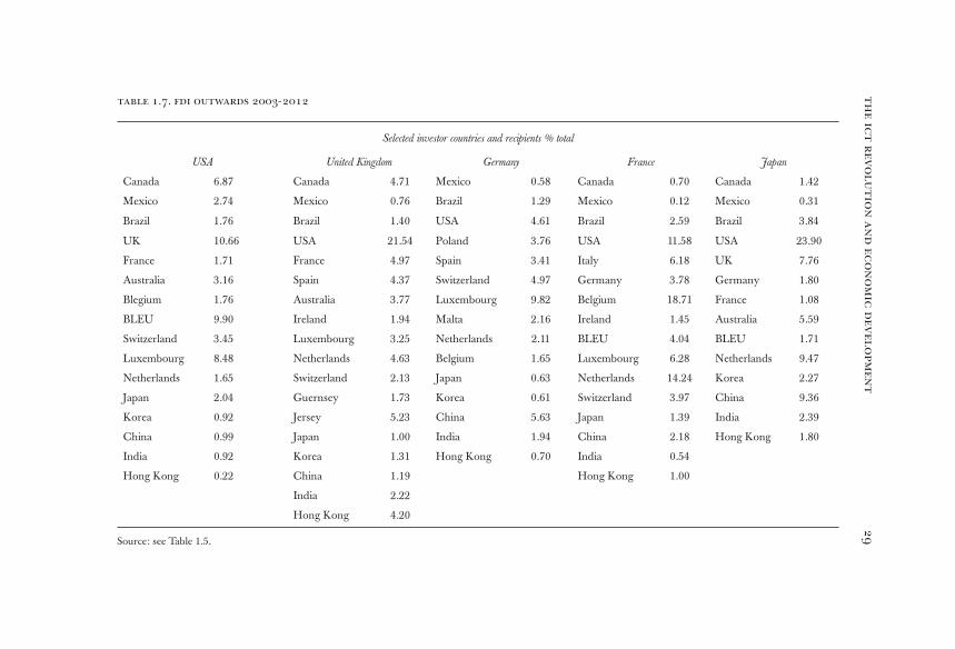
Let us start simply by analyzing the different countries that introduce FDI in China, India, Mexico, and Brazil. As seen in Table 1.7, China represents 1.0 % of the outward USA FDI flows in average from 2003 to
carlos obregón28
2012. The corresponding numbers are the UK 1.2%, Japan 9.4%, Germa-ny 5.6%, and France 2.2%. Of course, China received huge investments from Hong Kong. India represents 0.9% of the USA, 2.2% of the UK, 2.4% of Japan, 1.9% of Germany, and 0.5% of France. Mexico represents 2.7% of the USA (for Mexico, means 44.08% of what it receives), 0.8% of the UK, 0.3% of Japan, 0.6% of Germany and 0.1% of France. Brazil represents 1.8 % of the USA, 1.4% of the UK, 3.8% from Japan, 1.3% from Germany, and 2.6% from France.
table 1.6. growth rates. gdp per capita, ppp
(constant 2011 international dollars)
Period: 1990-2016 2008-2016 1990-2008 1990-2005 2005-2016
India 4.90 6.13 4.37 4.04 6.11
China 9.02 7.71 9.60 9.21 9.02
Mexico 1.12 0.63 1.35 1.30 0.87
Brazil 1.18 0.19 1.62 1.16 1.78
Source: World Bank DataBank, WDI, last updated 08/02/2017 (see Table 1.1).
These numbers are relevant, because they reveal the relative strength of the country to negotiate with its foreign investors. China is in a very good position due to the support of Hong Kong, which represents 4.2% of the UK, 1.8% of Japan, 1.0% of France, 0.7% of Germany, and 0.2% of the USA. China and Hong Kong are relatively powerful in front of Japan —its main creditor— and their well diverse sources of investors allowed them to put better conditions on the reception of FDI. Mexico, at the other extreme, is relatively weak in front of the USA; over concentrated on this country, both as source of foreign investment and destination of its exports. Does this explain why Mexico did not grow? It does not. We will see later on that the value added in exports is the same in China and Mexico, therefore the relative weaker negotiating capacity of Mexico does not show here. But what the previous numbers do show is that Mexico entered the ICT revolution through NAFTA and through USA and not as a conscious policy to benefit from the ICT revolution. This explains why Mexico did not offer excellent conditions like China’s to the global investors. Mexico thought that the NAFTA and sound neoclassical macroeconomic policies were enough to foster economic growth. It was wrong.
th
e i
ct
rev
olu
tio
n a
nd
ec
on
om
ic
dev
elo
pm
en
t2
9table 1.7. fdi outwards 2003-2012
Selected investor countries and recipients % total
USA United Kingdom Germany France Japan
Canada 6.87 Canada 4.71 Mexico 0.58 Canada 0.70 Canada 1.42
Mexico 2.74 Mexico 0.76 Brazil 1.29 Mexico 0.12 Mexico 0.31
Brazil 1.76 Brazil 1.40 USA 4.61 Brazil 2.59 Brazil 3.84
UK 10.66 USA 21.54 Poland 3.76 USA 11.58 USA 23.90
France 1.71 France 4.97 Spain 3.41 Italy 6.18 UK 7.76
Australia 3.16 Spain 4.37 Switzerland 4.97 Germany 3.78 Germany 1.80
Blegium 1.76 Australia 3.77 Luxembourg 9.82 Belgium 18.71 France 1.08
BLEU 9.90 Ireland 1.94 Malta 2.16 Ireland 1.45 Australia 5.59
Switzerland 3.45 Luxembourg 3.25 Netherlands 2.11 BLEU 4.04 BLEU 1.71
Luxembourg 8.48 Netherlands 4.63 Belgium 1.65 Luxembourg 6.28 Netherlands 9.47
Netherlands 1.65 Switzerland 2.13 Japan 0.63 Netherlands 14.24 Korea 2.27
Japan 2.04 Guernsey 1.73 Korea 0.61 Switzerland 3.97 China 9.36
Korea 0.92 Jersey 5.23 China 5.63 Japan 1.39 India 2.39
China 0.99 Japan 1.00 India 1.94 China 2.18 Hong Kong 1.80
India 0.92 Korea 1.31 Hong Kong 0.70 India 0.54
Hong Kong 0.22 China 1.19 Hong Kong 1.00
India 2.22
Hong Kong 4.20
Source: see Table 1.5.

carlos obregón30
table 1.8. country merchandise exports as percentage of world´s
merchandise exports
Year: 1950 1960 1970 1980 1990 2000 2008 2016
Brazil 2.19 0.98 0.86 0.99 0.90 0.85 1.22 1.16
Canada 4.87 4.48 5.30 3.33 3.66 4.28 2.82 2.45
China 0.89 1.98 0.73 0.89 1.78 3.86 8.85 13.15
France 4.97 5.28 5.71 5.70 6.21 5.07 3.81 3.14
Germany 3.21 8.78 10.80 9.47 12.07 8.54 8.95 8.40
Hong Kong 1.05 0.53 0.79 1.00 2.37 3.14 2.29 3.24
China & Hong Kong
1.94 2.51 1.52 1.89 4.14 7.00 11.14 16.39
India 1.85 1.02 0.64 0.42 0.51 0.66 1.21 1.65
Japan 1.33 3.12 6.09 6.41 8.24 7.42 4.84 4.04
Korea 0.04 0.02 0.26 0.86 1.86 2.67 2.61 3.11
Malaysia 1.62 0.91 0.53 0.64 0.84 1.52 1.23 1.19
Mexico 0.86 0.59 0.44 0.89 1.17 2.58 1.80 2.34
Singapore 1.62 0.87 0.49 0.95 1.51 2.13 2.09 2.07
Thailand 0.49 0.31 0.22 0.32 0.66 1.07 1.10 1.35
UK 1.02 8.16 6.13 5.41 5.31 4.42 2.92 2.57
USA 16.12 15.10 13.64 11.08 11.28 12.11 7.97 9.12
Source: World Trade Organization (WTO) database, http://stat.wto.org, consulted 10/08/2017.
Table 1.8 shows the ICT revolution from the point of view of merchan-dise exports. China went from 0.9% of global merchandise exports in 1980 to 1.8% in 1990 and an impressive 13.2% in 2016. Together with Hong Kong the number is 16.4%. A number substantially bigger than Germany, France and the UK together (14.1%) or than the sum of USA, Canada and Mexico (13.9%). From 1980 to 2016 most of the developed economies lost ground: the USA went down from 11.1% in 1980 to 9.1% in 2016, the UK from 5.4% to 2.6%, Germany from 9.5% to 8.4%, France from 5.7% to 3.1% and Japan from 6.4% to 4.0%. In the same period, India went from 0.4% to 1.7%, Mexico from 0.9% to 2.3% and Brazil from 1.0% to only 1.2%.
the ict revolution and economic development 31
table 1.9. merchandise imports as percentage of exports
Year: 1950 1960 1970 1980 1990 2000 2008 2016
UK 1.15 1.23 1.13 1.05 1.20 1.22 1.39 1.55
USA 0.96 0.83 0.98 1.14 1.31 1.61 1.69 1.55
Canada 1.03 1.04 0.85 0.92 0.97 0.88 0.92 1.07
Mexico 1.03 1.55 1.76 1.23 1.07 1.08 1.09 1.06
China 1.05 1.03 0.99 1.10 0.86 0.90 0.79 0.76
India 0.95 1.73 1.05 1.73 1.31 1.22 1.65 1.36
Japan 1.17 1.11 0.98 1.08 0.82 0.79 0.98 0.94
Germany 1.36 0.89 0.87 0.97 0.84 0.90 0.82 0.79
France 1.00 0.91 1.06 1.16 1.08 1.03 1.16 1.14
Brazil 0.80 1.15 1.04 1.24 0.72 1.06 0.92 0.77
Hong Kong 1.02 1.49 1.16 1.13 1.03 1.06 1.06 1.06
China & Hong Kong
1.04 1.13 1.08 1.12 0.96 0.97 0.85 0.82
Korea 2.35 10.75 2.37 1.27 1.07 0.93 1.03 0.82
Malaysia 0.54 0.77 0.83 0.83 0.99 0.83 0.79 0.89
Singapore 1.06 1.17 1.58 1.24 1.15 0.98 0.95 0.86
Thailand 0.69 1.12 1.83 1.42 1.43 0.90 1.01 0.90
Source: see Table 1.8.
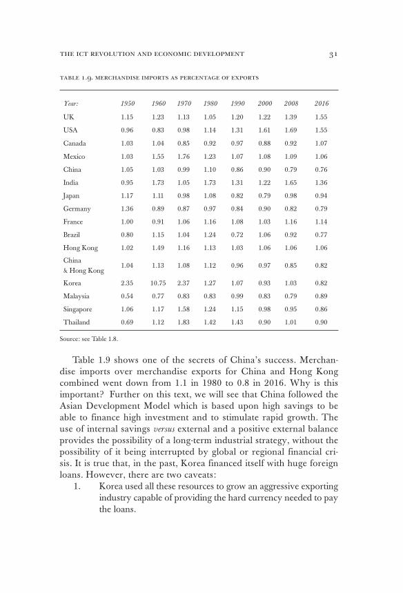
Table 1.9 shows one of the secrets of China’s success. Merchan-dise imports over merchandise exports for China and Hong Kong combined went down from 1.1 in 1980 to 0.8 in 2016. Why is this important? Further on this text, we will see that China followed the Asian Development Model which is based upon high savings to be able to finance high investment and to stimulate rapid growth. The use of internal savings versus external and a positive external balance provides the possibility of a long-term industrial strategy, without the possibility of it being interrupted by global or regional financial cri-sis. It is true that, in the past, Korea financed itself with huge foreign loans. However, there are two caveats:
1. Korea used all these resources to grow an aggressive exporting industry capable of providing the hard currency needed to pay the loans.
carlos obregón32
2. The Asian financial crisis at the end of the 1990s brought a hard lesson for the Asian economies —speculators hit hard, even the economies that had sound and healthy macro finan-cials— due to what is known as the contagious effect.
Therefore, having a trade surplus guarantees long-term stability —both through the lack of foreign investment needed to finance current account, and through the accumulation of huge foreign reserves.
Notice in Table 1.9 that merchandise imports over exports is less than one in 2016 for Japan, Korea, Singapore, Thailand, China, and China, plus Hong Kong. The strategy of the Asian Development Model started with Japan. See how Japan went down from 1.2 to 1.0 from 1950 to 1970. A trade surplus allows the country more sovereign control upon its long-term growth strategy, which, for both Japan and Germany, was a priority after the Second World War, and it continues to be. Notice Germany did the same as Japan; it went down from 1.4 in 1950 to 0.9 in 1970 and in 2016 it is at 0.8.
table 1.10. manufactured exports as percentage of merchandise exports
Year: 1990 2000 2008 2016
USA 74.1 82.7 74.0 63.4
UK 79.1 75.7 68.2 79.1
Japan 95.9 93.9 89.2 88.5
Germany 89.0 83.7 82.1 84.1
China 71.6 88.2 93.0 94.3*
Hong Kong 94.5 95.3 82.8 63.0
France 77.0 80.9 77.6 79.8
Korea 93.5 90.7 86.9 89.6*
Brazil 51.9 58.4 44.8 39.8
Mexico 43.5 85.5 73.6 83.0
India 70.7 77.8 62.8 73.1
Canada 58.8 65.3 47.0 54.5
Source: WDI DataBank, World Bank, see Table 1.1. Used 2015 for China and Korea (*) since 2016 data was not available.
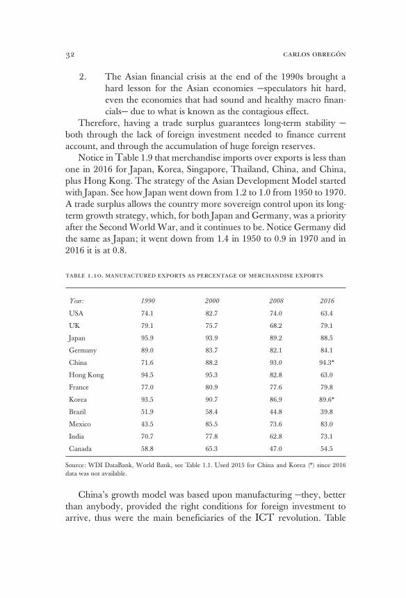
China’s growth model was based upon manufacturing —they, better than anybody, provided the right conditions for foreign investment to arrive, thus were the main beneficiaries of the ICT revolution. Table
the ict revolution and economic development 33
1.10 shows manufacture exports as a percentage of merchandise exports. While this indicator went down for many developed countries (with the exception of the UK and France) from 1990-2016 such as USA, Germa-ny, Canada, Japan, and even Korea, it increased rapidly in China. In that same table, by 1990 China had a 71.6% —already higher than Mexico or Brazil but similar to India. In 2015, the number was 94.3%. This number is higher than any other country’s, with Korea following at 89.6%, Japan at 88.5%, and Germany at 84.1%16. In the same period, India increased slightly, Brazil went down from 51.9% to 39.8%, and Mexico went up from 43.5% to an impressive 83.0%. This last fact brings us back to the question: why did Mexico not grow?
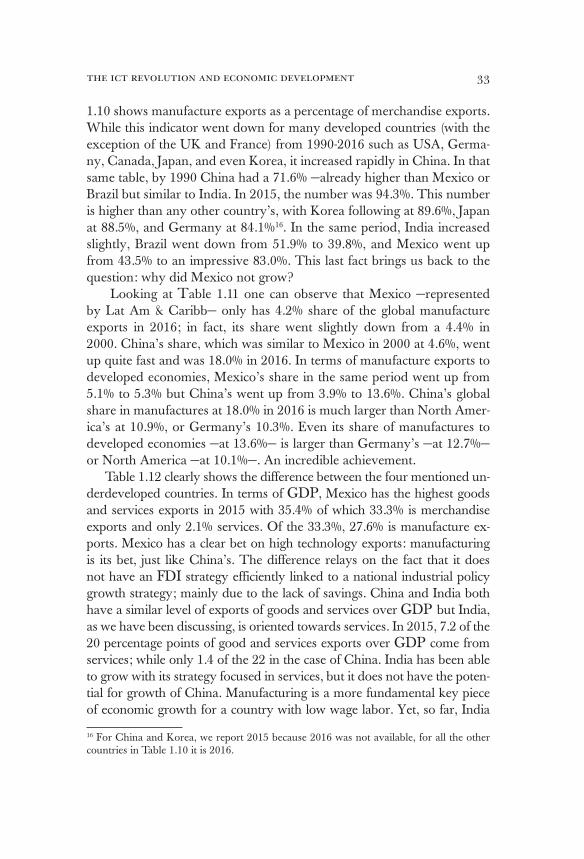
Looking at Table 1.11 one can observe that Mexico —represented by Lat Am & Caribb— only has 4.2% share of the global manufacture exports in 2016; in fact, its share went slightly down from a 4.4% in 2000. China’s share, which was similar to Mexico in 2000 at 4.6%, went up quite fast and was 18.0% in 2016. In terms of manufacture exports to developed economies, Mexico’s share in the same period went up from 5.1% to 5.3% but China’s went up from 3.9% to 13.6%. China’s global share in manufactures at 18.0% in 2016 is much larger than North Amer-ica’s at 10.9%, or Germany’s 10.3%. Even its share of manufactures to developed economies —at 13.6%— is larger than Germany’s —at 12.7%— or North America —at 10.1%—. An incredible achievement.
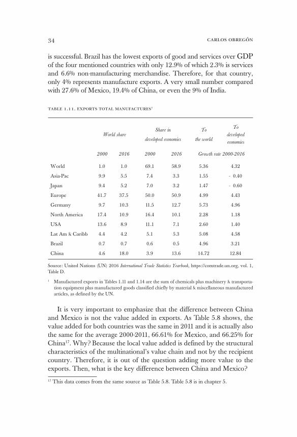
Table 1.12 clearly shows the difference between the four mentioned un-derdeveloped countries. In terms of GDP, Mexico has the highest goods and services exports in 2015 with 35.4% of which 33.3% is merchandise exports and only 2.1% services. Of the 33.3%, 27.6% is manufacture ex-ports. Mexico has a clear bet on high technology exports: manufacturing is its bet, just like China’s. The difference relays on the fact that it does not have an FDI strategy efficiently linked to a national industrial policy growth strategy; mainly due to the lack of savings. China and India both have a similar level of exports of goods and services over GDP but India, as we have been discussing, is oriented towards services. In 2015, 7.2 of the 20 percentage points of good and services exports over GDP come from services; while only 1.4 of the 22 in the case of China. India has been able to grow with its strategy focused in services, but it does not have the poten-tial for growth of China. Manufacturing is a more fundamental key piece of economic growth for a country with low wage labor. Yet, so far, India
16 For China and Korea, we report 2015 because 2016 was not available, for all the other countries in Table 1.10 it is 2016.
carlos obregón34
is successful. Brazil has the lowest exports of good and services over GDP of the four mentioned countries with only 12.9% of which 2.3% is services and 6.6% non-manufacturing merchandise. Therefore, for that country, only 4% represents manufacture exports. A very small number compared with 27.6% of Mexico, 19.4% of China, or even the 9% of India.
table 1.11. exports total manufactures1
World shareShare in
developed economies
To
the world
To
developed
economies
2000 2016 2000 2016 Growth rate 2000-2016
World 1.0 1.0 69.1 58.9 5.36 4.32
Asia-Pac 9.9 5.5 7.4 3.3 1.55 - 0.40
Japan 9.4 5.2 7.0 3.2 1.47 - 0.60
Europe 41.7 37.5 50.0 50.9 4.99 4.43
Germany 9.7 10.3 11.5 12.7 5.73 4.96
North America 17.4 10.9 16.4 10.1 2.28 1.18
USA 13.6 8.9 11.1 7.1 2.60 1.40
Lat Am & Caribb 4.4 4.2 5.1 5.3 5.08 4.58
Brazil 0.7 0.7 0.6 0.5 4.96 3.21
China 4.6 18.0 3.9 13.6 14.72 12.84
Source: United Nations (UN) 2016 International Trade Statistics Yearbook, https://comtrade.un.org, vol. 1, Table D.
1 Manufactured exports in Tables 1.11 and 1.14 are the sum of chemicals plus machinery & transporta-tion equipment plus manufactured goods classified chiefly by material & miscellaneous manufactured articles, as defined by the UN.
It is very important to emphasize that the difference between China and Mexico is not the value added in exports. As Table 5.8 shows, the value added for both countries was the same in 2011 and it is actually also the same for the average 2000-2011, 66.61% for Mexico, and 66.25% for China17. Why? Because the local value added is defined by the structural characteristics of the multinational’s value chain and not by the recipient country. Therefore, it is out of the question adding more value to the exports. Then, what is the key difference between China and Mexico?
17 This data comes from the same source as Table 5.8. Table 5.8 is in chapter 5.
the ict revolution and economic development 35
table 1.12. exports as percentage of gdp (2015)
Manufactured exports Merchandise exportsExports
goods & services
Exports
services
USA 5.4 8.3 12.6 4.2
UK 12.6 16.1 27.6 11.5
Japan 12.6 14.3 17.6 3.4
Germany 33.3 39.5 46.8 7.3
China 19.4 20.6 22.0 1.4
Hong Kong 108.6 165.1 201.6 36.5
France 16.5 20.9 30.0 9.1
Korea 34.3 38.2 45.9 7.7
Brazil 4.0 10.6 12.9 2.3
Mexico 27.6 33.3 35.4 2.1
India 9.0 12.8 20.0 7.2
Canada 13.8 26.3 31.6 5.3
Source: WDI DataBank, last updated 08/02/2017 (see Table 1.1).
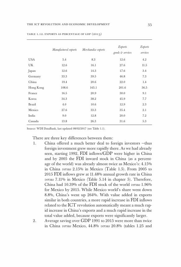
There are three key differences between them: 1. China offered a much better deal to foreign investors —thus
foreign investment grew more rapidly there. As we had already seen, starting 1992, FDI inflows/GDP were higher in China and by 2005 the FDI inward stock in China (as a percent-age of the world) was already almost twice as Mexico’s: 4.15% in China versus 2.15% in Mexico (Table 1.5). From 2005 to 2015 FDI inflows grew at 11.48% annual growth rate in China versus 7.11% in Mexico (Table 5.14 in chapter 5). Therefore, China had 10.39% of the FDI stock of the world versus 1.96% for Mexico by 2015. While Mexico world’s share went down 8.8%, China’s went up 264%. With value added in exports similar in both countries, a more rapid increase in FDI inflows related to the ICT revolution automatically meant a much rap-id increase in China’s exports and a much rapid increase in the total value added, because exports were significantly larger.
2. Average saving over GDP 1991 to 2015 were more than twice in China versus Mexico, 44.8% versus 20.8% (tables 1.25 and
carlos obregón36
1.26)18. The high savings in China explain its growth in the tra-ditional sense of a Solow’s model. But there is more than this. The high savings mean the possibility of growing local com-panies that can learn from foreign investors; Romer’s transfer of knowledge becomes a reality. The problem with Mexico is that its low savings only allows it to grow enough to bring value added to exports and to have a low growth for the rest of the economy. Under these circumstances: it is not possible to develop a national industrial strategy like the one China has; and it is not possible either, to develop champion national companies capable to compete globally.
3. China used the Asian Development Model and had a specific industrial strategy, based upon high savings, high exports, and a positive external balance. Therefore, China accumulated huge reserves. In a first stage, it protected its local industries through restricting imports, and in a second stage —after joining the WTO in 2001—, protected its industries by devaluating the cur-rency. China’s model recognized the fact that economic growth requires large savings and that FDI was not going to solve the problem by itself. Instead, Mexico followed the neoclassical eco-nomic model and assumed that its low local savings were going to be compensated with huge FDI, which not happened. FDI arrived to create value for international chains due to the ICT revolution, not to substitute local savings. Mexico had free trade and a free-floating exchange rate waiting for the FDI that never arrived in the amounts expected by the neoclassical theory. Fi-nally, even though Mexico managed to have a trade surplus with the USA, it had an even higher deficit with the rest of the world (see Table 1.17). Therefore, Mexico was unable to de-velop a truly competitive national industry.
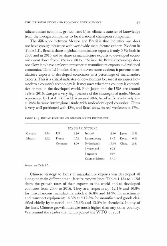
In terms of income producing, China has become even more important for the USA than Mexico (see Table 1.13). In 2015, explained 2.4% of the in-come received by USA FDI’s investors while Mexico only explained 1.9%.
There is however, some hope for Mexico because, while Brazil and Argentina did not enter the ICT revolution, Mexico did. With that ad-vantage, it could be more aggressive and attract more foreign investment. If in addition Mexico increases its savings substantially and implements a national industrial policy, it will be able to obtain two goals: a) a sig-
18 For Mexico it is 1991-2016.
the ict revolution and economic development 37
nificant faster economic growth, and b) an efficient transfer of knowledge from the foreign companies to local national champion companies.
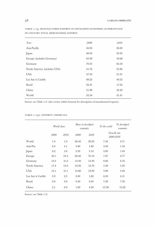
The difference between Mexico and Brazil is that the latter one does not have enough presence with worldwide manufacture exports. Evident in Table 1.11, Brazil’s share in global manufacture exports is only 0.7% both in 2000 and in 2016 and its share in manufacture exports to developed econo-mies went down from 0.6% in 2000 to 0.5% in 2016. Brazil’s technology does not allow it to have a relevant presence in manufacture exports to developed economies. Table 1.14 makes this point even more evident; it presents man-ufacture exports to developed economies as a percentage of merchandise exports. This is a critical indicator of development because it measures how modern a country’s technology is. It measures whether a country is competi-tive or not, in the developed world. Both Japan and the USA are around 32% in 2016, Europe is very high because of the intraregional trade, Mexico represented by Lat Am & Caribb is around 40%, Asia-Pacific is relatively low at 26% because intraregional trade with underdeveloped countries; China is very well positioned with 42%, and Brazil show its real weakness at 17%.
table 1.13. income received on foreign direct investment
USA 2015 % OF TOTAL
Canada 4.74 UK 9.80 Ireland 11.40 Japan 2.31
Mexico 1.92 France 0.52 Luxembourg 8.45 Korea 0.66
Germany 1.00 Netherlands 17.06 China 2.44
Switzerland 6.31
Singapore 0.57
Cayman Islands 5.49
Source: see Table 1.5.
Chinese strategy to focus in manufacture exports was developed all along the main different manufacture exports lines. Tables 1.15a to 1.15d show the growth rates of their exports to the world and to developed countries from 2000 to 2016. They are, respectively: 12.1% and 10.8% for miscellaneous manufacture articles; 16.8% and 14.9% for machinery and transport equipment; 14.3% and 12.3% for manufactured goods clas-sified chiefly by material; and 15.6% and 13.2% in chemicals. In any of the lines, Chinese growth rates are much higher than any other country. We remind the reader that China joined the WTO in 2001.
carlos obregón38
table 1.14. manufactured exports to developed economies as percentage
of country total merchandise exports
Year: 2000 2016
Asia-Pacific 44.36 26.63
Japan 48.59 33.03
Europe (includes Germany) 65.99 59.68
Germany 70.35 62.18
North America (includes USA) 51.76 35.84
USA 47.59 31.91
Lat Am & Caribb 48.22 40.32
Brazil 34.45 17.02
China 51.98 42.20
World 52.50 41.41
Source: see Table 1.11 (also review table´s footnote for description of manufactured exports).
table 1.15a. exports: chemicals
World shareShare in developed
economiesTo the world
To developed
economies
2000 2016 2000 2016Growth rate
2000-2016
World 1.0 1.0 66.43 58.30 7.42 6.71
Asia-Pac 6.9 4.1 3.90 1.80 3.92 1.50
Japan 6.2 3.6 3.30 3.14 3.85 1.04
Europe 56.1 53.2 69.40 70.10 7.07 6.77
Germany 12.3 11.2 14.30 14.40 6.82 6.76
North America 17.4 13.0 16.30 12.70 5.49 5.05
USA 14.1 11.1 12.80 10.00 5.80 5.04
Lat Am & Caribb 2.9 2.5 2.00 1.82 6.39 6.11
Brazil 0.6 0.6 0.40 0.40 7.29 7.36
China 2.1 6.9 1.60 4.20 15.58 13.22
Source: see Table 1.11.
the ict revolution and economic development 39
table 1.15b. exports: manufactured goods classified chiefly by material
World shareShare in developed
economiesTo the world
To developed
economies
2000 2016 2000 2016 Growth rate 2000-2016
World 1.0 1.0 65.7 53.8 5.24 3.93
Asia-Pac 6.5 4.4 3.3 1.9 2.63 - 0.32
Japan 5.4 3.7 2.4 1.4 2.85 0.48
Europe 45.0 35.6 57.2 52.0 3.71 3.31
Germany 8.8 7.9 11.2 11.7 4.50 4.19
North America 12.9 9.1 13.7 9.5 3.00 1.60
USA 8.3 6.7 7.1 5.5 3.87 2.35
Lat Am & Caribb
4.9 4.3 4.8 4.2 4.42 3.04
Brazil 1.3 1.2 1.2 1.0 4.59 3.17
China 4.9 18.3 3.4 11.7 14.25 12.32
Source: see Table 1.11.
In chemical exports —Table 1.15a—, the USA and Germany have a clear lead; however, USA world share went down from 14.1% in 2000 to 11.1% in 2016 and Germany went down from 12.3% to 11.2% while China grew from 2.1% to 6.9%. China’s 2016 global share is still significantly lower than those of the USA and Germany, but growing faster at 15.6% per year versus 6.8% for Germany and 5.8% for the USA. The lead of the latter two is even clearer in chemical exports to developed economies, with the US standing at 10.0% share in 2016 and Germany at 14.4% versus only 4.2% for China. However, the share of the USA went down from 12.8% in 2000, while China went up from 1.6%. Germany maintained its share at around 14.3%, but again its growth rate is substantially lower than China’s, 6.8% versus 13.2%. Although the successful Asian country is behind in chemical exports, it is catching up rapidly.
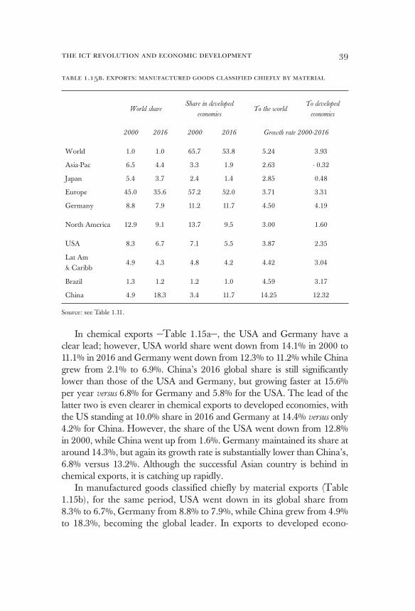
In manufactured goods classified chiefly by material exports (Table 1.15b), for the same period, USA went down in its global share from 8.3% to 6.7%, Germany from 8.8% to 7.9%, while China grew from 4.9% to 18.3%, becoming the global leader. In exports to developed econo-
carlos obregón40
mies, the USA went down from 7.1% to 5.5%, and Germany increased its share from 11.2 to 11.7%, but China grew from 3.4% to 11.7% also becoming in this line the global leader.
table 1.15c. exports: machinery and transport equipment
World shareShare in developed
economies
To
the world
To developed
economies
2000 2016 2000 2016 Growth rate 2000-2016
World 1.0 1.0 68.7 58.4 4.60 3.54
Asia-Pac 12.9 7.4 10.6 5.4 1.04 - 0.69
Japan 12.6 6.2 10.3 5.3 0.98 - 0.71
Europe 38.9 38.2 46.4 47.8 4.49 3.73
Germany 10.4 12.1 12.4 14.3 5.58 4.45
North America 20.0 11.6 18.6 10.2 1.09 - 0.29
USA 15.7 9.4 12.7 6.1 1.28 - 0.40
Lat Am & Caribb 4.7 5.2 6.0 7.5 5.32 4.95
Brazil 0.6 0.6 0.5 0.5 5.22 3.15
China 3.2 18.4 2.6 13.6 16.80 14.90
Source: see Table 1.11.
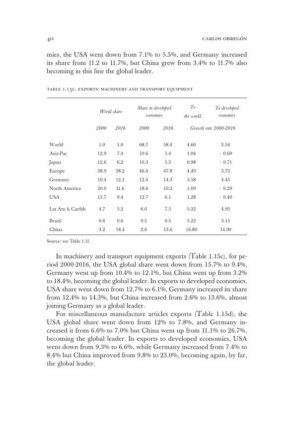
In machinery and transport equipment exports (Table 1.15c), for pe-riod 2000-2016, the USA global share went down from 15.7% to 9.4%, Germany went up from 10.4% to 12.1%, but China went up from 3.2% to 18.4%, becoming the global leader. In exports to developed economies, USA share went down from 12.7% to 6.1%, Germany increased its share from 12.4% to 14.3%, but China increased from 2.6% to 13.6%, almost joining Germany as a global leader.
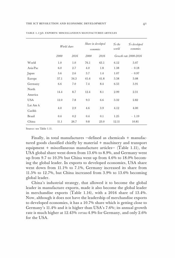
For miscellaneous manufacture articles exports (Table 1.15d), the USA global share went down from 12% to 7.8%, and Germany in-creased it from 6.6% to 7.0% but China went up from 11.1% to 26.7%, becoming the global leader. In exports to developed economies, USA went down from 9.3% to 6.6%, while Germany increased from 7.4% to 8.4% but China improved from 9.8% to 23.0%, becoming again, by far, the global leader.
the ict revolution and economic development 41
table 1.15d. exports: miscellaneous manufactured articles
World shareShare in developed
economies
To the
world
To developed
economies
2000 2016 2000 2016 Growth rate 2000-2016
World 1.0 1.0 76.1 63.1 6.12 5.07
Asia-Pac 6.0 2.7 4.0 1.8 1.38 - 0.18
Japan 5.6 2.6 3.7 1.4 1.07 - 0.97
Europe 37.1 34.3 41.6 41.8 5.58 5.08
Germany 6.6 7.0 7.4 8.4 6.53 5.91
North
America14.4 8.7 12.4 8.1 2.99 2.31
USA 12.0 7.8 9.3 6.6 3.32 2.82
Lat Am &
Caribb4.0 2.9 4.6 3.9 4.12 4.00
Brazil 0.4 0.2 0.4 0.1 1.25 - 1.19
China 11.1 26.7 9.8 23.0 12.11 10.81
Source: see Table 1.11.
Finally, in total manufactures —defined as chemicals + manufac-tured goods classified chiefly by material + machinery and transport equipment + miscellaneous manufacture articles— (Table 1.11), the USA global share went down from 13.6% to 8.9%, and Germany went up from 9.7 to 10.3% but China went up from 4.6% to 18.0% becom-ing the global leader. In exports to developed economies, USA share went down from 11.1% to 7.1%, Germany increased its share from 11.5% to 12.7%, but China increased from 3.9% to 13.6% becoming global leader.
China’s industrial strategy, that allowed it to become the global leader in manufacture exports, made it also become the global leader in merchandise exports (Table 1.16), with a 2016 share of 13.4%. Now, although it does not have the leadership of merchandise exports to developed economies, it has a 10.7% share which is getting close to Germany’s 11.4% and it is higher than USA’s 7.6%; its annual growth rate is much higher at 12.43% versus 4.9% for Germany, and only 2.6% for the USA.

carlos obregón42
table 1.16. exports: total merchandise trade
World shareShare in developed
economies
To the
world
To developed
economies
2000 2016 2000 2016 Growth rate 2000-2016
World 1.00 1.0 6.90 5.24 5.87 4.36
Asia-Pac 8.80 5.5 6.50 3.50 2.82 0.48
Japan 7.50 4.1 5.60 2.70 1.87 - 0.29
Europe 39.80 35.3 48.50 49.10 5.09 4.44
Germany 8.60 8.5 10.50 11.40 5.77 4.90
North America 16.70 11.6 16.00 11.50 3.53 2.22
USA 12.30 9.2 10.00 7.60 3.96 2.57
Lat Am & Caribb 5.60 5.5 5.90 6.30 5.76 4.79
Brazil 0.87 1.2 0.77 0.78 7.87 4.47
China 3.90 13.4 3.30 10.70 14.31 12.43
Source: see Table 1.11.
An interesting question is who exports to whom. Table 1.17 pres-ents merchandise exports over total world’s merchandise exports for several countries or regions. China represents 13.2% of total merchan-dise exports in 2015 and only 9.8% of total imports19. We can see that, even though the USA is its main customer, China has its exports very well diversified. Of the 13.2%, 7.2% goes to several other countries: 2.4% to the USA, 2.1% to the European Union (EU) and 0.8% to Japan. The EU represents 15.4% of total global merchandise exports in the same year and 14.8% of global imports. Its main customer is also the US with 3.1%, followed by China with 1.4%, Switzerland with 1.3%, and Russia with 0.6%. Japan represents 4.0% of global merchandise exports and 3.7% of global imports. USA is also its main customer with 0.8 %, China being second with 0.7%, followed by EU with 0.5, and Korea with 0.3. The USA represents 9.1% of global mer-chandise exports and 13.9% of global imports; its consumption pro-
19 Before, we mentioned 13.4%; this is acceptable because tables 1.16 and 1.17 come from different sources, this comment applies for the other countries. In particular, the European Union in Table 1.17 excludes intratrade while Europe in Table 1.16 does not.
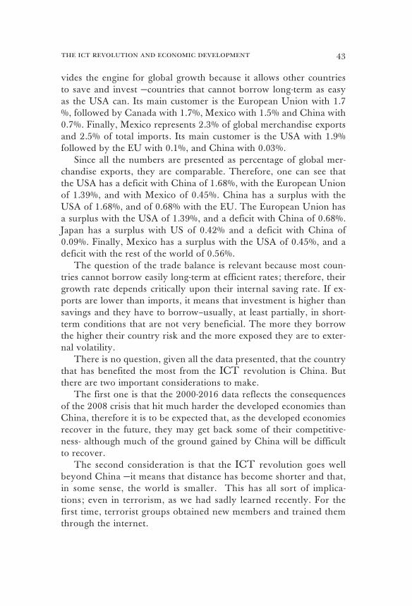
the ict revolution and economic development 43
vides the engine for global growth because it allows other countries to save and invest —countries that cannot borrow long-term as easy as the USA can. Its main customer is the European Union with 1.7 %, followed by Canada with 1.7%, Mexico with 1.5% and China with 0.7%. Finally, Mexico represents 2.3% of global merchandise exports and 2.5% of total imports. Its main customer is the USA with 1.9% followed by the EU with 0.1%, and China with 0.03%.
Since all the numbers are presented as percentage of global mer-chandise exports, they are comparable. Therefore, one can see that the USA has a deficit with China of 1.68%, with the European Union of 1.39%, and with Mexico of 0.45%. China has a surplus with the USA of 1.68%, and of 0.68% with the EU. The European Union has a surplus with the USA of 1.39%, and a deficit with China of 0.68%. Japan has a surplus with US of 0.42% and a deficit with China of 0.09%. Finally, Mexico has a surplus with the USA of 0.45%, and a deficit with the rest of the world of 0.56%.
The question of the trade balance is relevant because most coun-tries cannot borrow easily long-term at efficient rates; therefore, their growth rate depends critically upon their internal saving rate. If ex-ports are lower than imports, it means that investment is higher than savings and they have to borrow–usually, at least partially, in short-term conditions that are not very beneficial. The more they borrow the higher their country risk and the more exposed they are to exter-nal volatility.
There is no question, given all the data presented, that the country that has benefited the most from the ICT revolution is China. But there are two important considerations to make.
The first one is that the 2000-2016 data reflects the consequences of the 2008 crisis that hit much harder the developed economies than China, therefore it is to be expected that, as the developed economies recover in the future, they may get back some of their competitive-ness- although much of the ground gained by China will be difficult to recover.
The second consideration is that the ICT revolution goes well beyond China —it means that distance has become shorter and that, in some sense, the world is smaller. This has all sort of implica-tions; even in terrorism, as we had sadly learned recently. For the first time, terrorist groups obtained new members and trained them through the internet.
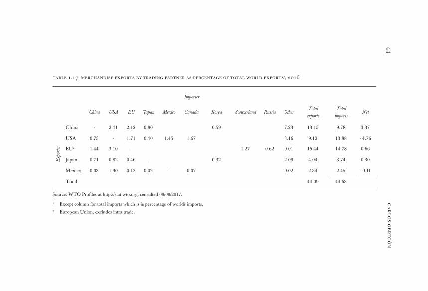
ca
rlo
s o
br
eg
ón
44
table 1.17. merchandise exports by trading partner as percentage of total world exports1, 2016
Importer
China USA EU Japan Mexico Canada Korea Switzerland Russia OtherTotal
exports
Total
importsNet
Exp
orte
r
China - 2.41 2.12 0.80 0.59 7.23 13.15 9.78 3.37
USA 0.73 - 1.71 0.40 1.45 1.67 3.16 9.12 13.88 - 4.76
EU2 1.44 3.10 - 1.27 0.62 9.01 15.44 14.78 0.66
Japan 0.71 0.82 0.46 - 0.32 2.09 4.04 3.74 0.30
Mexico 0.03 1.90 0.12 0.02 - 0.07 0.02 2.34 2.45 - 0.11
Total 44.09 44.63
Source: WTO Profiles at http://stat.wto.org, consulted 08/08/2017.
1 Except column for total imports which is in percentage of world´s imports.2 European Union, excludes intra trade.
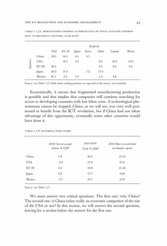
the ict revolution and economic development 45
table 1.17a. merchandise exports as percentage of total country exports
sent to recipient country, year 2016
Recipients
Exp
orte
rs
USA EU 28 Japan Korea China Canada Mexico
China 18.3 16.1 6.1 4.5 -
USA - 18.7 4.4 8.0 18.3 15.9
EU 28 20.1 - 9.3 8.2 4.0
Japan 20.2 11.4 - 7.2 17.6
Mexico 81.1 5.2 1.0 1.4 2.8 -
Source: see Table 1.17. Only main trading partners, as reported in the source, are included.
Economically, it means that fragmented manufacturing production is possible and that implies that companies will continue searching for access to developing countries with low labor costs. A technological phe-nomenon cannot be stopped. China, as we will see, was very well posi-tioned to benefit from the ICT revolution, but if China had not taken advantage of this opportunity, eventually some other countries would have done it.
table 1.18. external indicators
2016 Current account
balance % GDP
2014-2016
Trade % GDP
2016 Share in world total
merchandise exports
China 1.8 20.0 13.15
USA - 2.6 13.9 9.12
EU 28 2.4 16.8 15.44
Japan 3.9 17.7 4.04
Mexico - 2.7 35.7 2.34
Source: see Table 1.17.
We must answer two critical questions. The first one: why China? The second one: is China today really an economic competitor of the size of the USA or not? In this section, we will answer the second question, leaving for a section below the answer for the first one.
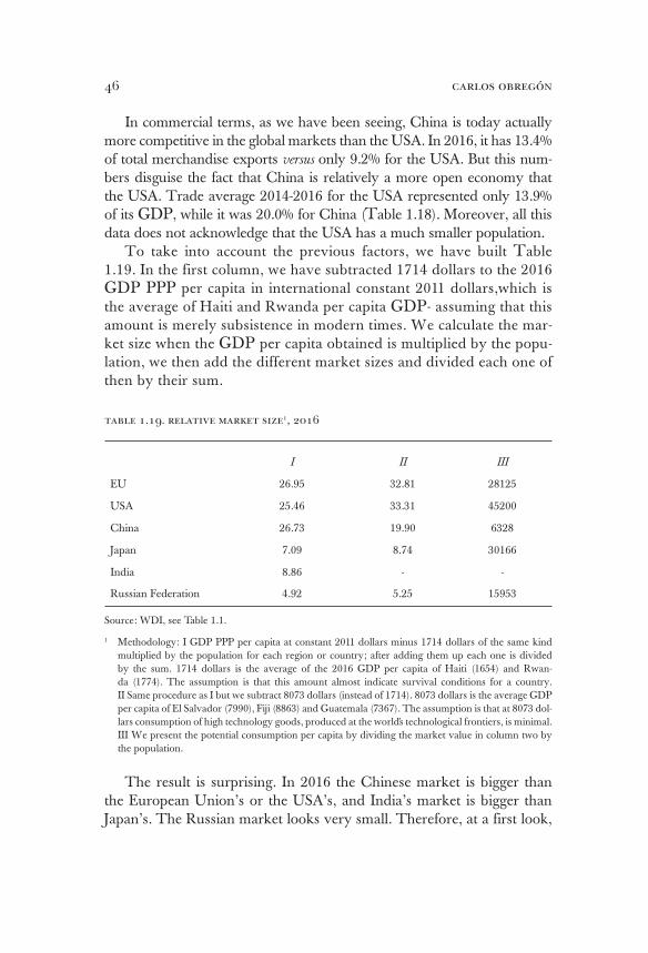
carlos obregón46
In commercial terms, as we have been seeing, China is today actually more competitive in the global markets than the USA. In 2016, it has 13.4% of total merchandise exports versus only 9.2% for the USA. But this num-bers disguise the fact that China is relatively a more open economy that the USA. Trade average 2014-2016 for the USA represented only 13.9% of its GDP, while it was 20.0% for China (Table 1.18). Moreover, all this data does not acknowledge that the USA has a much smaller population.
To take into account the previous factors, we have built Table 1.19. In the first column, we have subtracted 1714 dollars to the 2016 GDP PPP per capita in international constant 2011 dollars,which is the average of Haiti and Rwanda per capita GDP- assuming that this amount is merely subsistence in modern times. We calculate the mar-ket size when the GDP per capita obtained is multiplied by the popu-lation, we then add the different market sizes and divided each one of then by their sum.
table 1.19. relative market size1, 2016
I II III
EU 26.95 32.81 28125
USA 25.46 33.31 45200
China 26.73 19.90 6328
Japan 7.09 8.74 30166
India 8.86 - -
Russian Federation 4.92 5.25 15953
Source: WDI, see Table 1.1.
1 Methodology: I GDP PPP per capita at constant 2011 dollars minus 1714 dollars of the same kind multiplied by the population for each region or country; after adding them up each one is divided by the sum. 1714 dollars is the average of the 2016 GDP per capita of Haiti (1654) and Rwan-da (1774). The assumption is that this amount almost indicate survival conditions for a country. II Same procedure as I but we subtract 8073 dollars (instead of 1714). 8073 dollars is the average GDP per capita of El Salvador (7990), Fiji (8863) and Guatemala (7367). The assumption is that at 8073 dol-lars consumption of high technology goods, produced at the world´s technological frontiers, is minimal. III We present the potential consumption per capita by dividing the market value in column two by the population.
The result is surprising. In 2016 the Chinese market is bigger than the European Union’s or the USA’s, and India’s market is bigger than Japan’s. The Russian market looks very small. Therefore, at a first look,
the ict revolution and economic development 47
it seems unquestionable that China is becoming an adversary of such di-mensions that the United States has not had for the last century or more, but there are some caveats.
In the second column, using a similar procedure, to the GDP PPP per capita in international constant 2011 dollars we have subtracted 8073 dollars, which is the average of El Salvador, Guatemala, and Fiji GDP’s per capita. The assumption here is that, at 8073 dollars GDP per capita, there is little margin for the consumption of sophisticated technological goods —defined as those produced at the technological frontier.
Now India disappears because its GDP per capita is less than 8073 dol-lars. Nevertheless, China does not; it’s GDP is still more than twice Japan’s and it is 60% the USA’s. This indicator is relevant because it shows that China, while important, is still far away from being able to lead the world as the global consumer of sophisticated goods. In the last column, we have presented the per capita potential consumption related to column two by dividing the value of the market by the population. This last column shows that, in terms of very sophisticated products, the USA is the key market in the world followed by the European Union and Japan. In per capita consumption terms, China looks small —around 40% of the Russian Fed-eration. Therefore, technological progress still depends critically on the con-sumption of the middle class of the USA, the European Union, and Japan. Therefore, the answer to the second question is that China is not yet today a match for the USA. It will take many years for China to get where the USA is. But clearly, China is becoming increasingly important.
There are some key factors to take into account in this adversarial re-lation. The USA cannot stopt the ICT revolution; trade policies against China will hurt the latter but will not benefit the former. When the Clin-ton administration launched a set of adversarial trade policies against Japan it hurt this country, but it did not benefit the USA —others took Japan’s place, and the trade deficit and competitive position of the USA remained the same. In fact, the risk —and it is a huge one— is that protec-tionist commercial policies will end up moving away the USA from the privilege competitive international position that it enjoys today.
The ICT technology opportunities will be exploited anyhow. If the USA decides to produce with higher local salaries, it will be replaced very soon from the global leadership. The solution for the USA as a glob-al technological leader is to move forward; trying to move backwards will not work. It should concentrate in its competitive advantages as the leader in the ICT technology, the leader in global finances, the leader
carlos obregón48
innovator of top-line sophisticated technological goods, and as the leader consumer of high technological products.
As for China, it has problems of its own. The most critical question in China is political: will a soft authoritarian regime adapting itself to econom-ic concerns suffice in the future? Alternatively, will the growing economic middle class, more and more influenced by the West because of the commu-nication easiness provided by the ICT revolution, compete for the power with the high classes? No body knows the answer, but what is sure is that for the leaders it will be increasingly difficult to manage political pressures.
In economic issues, the question is whether China can create an en-gine of growth of its own, and if it can abandon the old model of huge savings and high domestic fixed asset investment for a new model with a middle-class supporting, domestic, consumer expense. Can China create a dynamic middle-class consumer that will not compete for the political power? No body has done it before; we will have to see.
In terms of exports, as the salaries increase in China and other poor coun-tries enter the ICT revolution, China needs to move upscale in the value added chain. It needs to promote innovation, as Japan and South Korea did. This seems a less difficult task to achieve than the previously mentioned.
China faces many other challenges like cleaning the environment, in-come inequality, and reforming the financial system and the state-owned enterprises, but perhaps the weakest point for China is its demography. It is changing from a young society to an aging one. That means that the working age population is starting to go down. In addition, the growing old population will put pressure for more public goods20. Will China succeed? No body knows, but what is clear is that it has many obstacles to overcome before it can really compete for the global leadership with the USA.
Immigration and the ICT Revolution
Ricardo developed the principle of competitive advantage, which is still today the main pillar on which neoclassical contemporary economic trade theory rest. The idea is simple: each country should specialize pro-ducing those goods for which it has a competitive advantage whether it is cheap labor, abundant land or anything else. This is the principle behind
20 For a good account of several issues to consider in China’s future, look at Shambaugh, D. 2016.
the ict revolution and economic development 49
the idea of free trade global benefits. It is also the principle in the Wash-ington Consensus proposal that those underdeveloped economies that establish open borders and free prices should develop (because capital looking for cheap labor should go to those countries and therefore they should develop). As we have just seen, it did not happen. Given all sorts of institutional constrains, it was too risky and expensive to produce in the developing economies, therefore, most of the capital stayed in the industrial countries, but this meant producing with expensive labor.
The ICT revolution made it possible for the developed nations com-petitive advantage (know-how) to move into underdeveloped countries avoiding the traditional developing countries institutional constrains; be-cause it did not matter anymore what happened in the developing coun-try as a whole.
The only relevant factors were the conditions under which the frag-ments of the manufacture production are received by the host country. Such conditions represent a lower risk than a transfer of the whole invest-ment process. In these new technological scenario, it became irrelevant whether tariffs in general were low or not in the host country. It was no longer a question of capital moving into the developing country —just know-how of a fragment of production will move. This is why traditional neoclassical trade theory could not explain any longer what was happen-ing, and the reason Mexico did not grow and China did.
Migration can be understood as the movement of one nation’s com-petitive advantage —labor— to another nation. As it is well known, the movement of labor from England to United States’ abundant lands was this country’s fundamental source of growth, particularly after the steam revolution made transportation more affordable.
Given the fact that global tariffs are already very low by historical standards, some authors have argued that the next productivity wave will no longer be associated with more trade, but that it could come from more open migration policies21. However, in the real world, anti-migration poli-cies have become more and more successful. The question is: why?
Migration can be thought as an extension of traditional trade theory. The idea of why it could be a source of future global productivity is very simple. Given the fact that global tariffs are already very low, trade is already near its maximum potential to promote global growth. And given the fact that the developing countries constrains will not disappear in the foreseeable future, most of the capital transfers that had to occur
21 See for example Rodrick 2011, p. 266.
carlos obregón50
also mostly happened already; the capital that could or would migrate has almost done it already. Then, it makes sense that the next wise global policy should be open migration. This will furthermore exploit competi-tive advantages by bringing abundant labor into the developed countries owning capital and know–how. The problem with this way of thinking is that it is pre-ICT.
The ICT revolution can be thought as reverse migration: instead of labor going to the countries with know-how, the know-how goes to the selected group of countries which offer abundant labor. Moreover, once the firms can go into the developing economies through fragmented pro-duction and enjoy the economic advantage of cheap abundant labor, they are no longer interested in cheap labor at home. In fact, migration from the firm’s point of view is an inferior solution, because bringing labor to the developed country is costlier. If migration is based in temporary permits to avoid the migrants from obtaining the full-blown benefits re-lated to the labor conditions in the developed economies, it implies huge administrative, training and transportation costs. If migration is based upon permanent permits, migrants soon will acquire the full-blown ben-efits related to the native workers of the developed nations and labor will become more expensive.
Politically, given the predominant humanistic ideology in the devel-oped countries, eventually it becomes very difficult to sustain in a perma-nent basis two distinct classes of workers. In any case, it is unavoidable that legalizing migrant workers, whether through permanent or transi-tory permits, will become more expensive. The ICT revolution provid-ed the solution through reverse migration. Workers stay in their own countries with their traditional low paid conditions, and know-how goes to them. In the past, the firms were doing pro-migration lobbying, and this was the key element that produced the political balanced required for promigration reforms to be approved. The ICT revolution has un-settled this balance in two ways: first, firms are no longer interested in pro-migration lobbying22; second, the success of fragmented production has meant that workers previously employed in a manufacture process in the developed countries have become unemployed, and many of them have joined the groups that had traditionally supported anti-migration policies —particularly after the 2008 crisis. Traditional trade competitive advantages and migration are still important sources of productivity for the global economy, but they are no longer the key to sustain significant
22 See Peters 2017, who empirically shows that this is the case.
the ict revolution and economic development 51
global productivity increases in the future. The new key is the ICT revo-lution because the world has changed.
why china and how do economic development occurs?
In order to answer in a proper way the first question: why China? We need to fully understand the implications of the ICT revolution and to this purpose it is good to review economic history. Which teaches us two lessons. First, technological revolutions always deeply change human soci-eties. Second, institutions are not always ready to accept the implications of the new coming technology; when they resist, it ends up being very damag-ing for the economic development of those countries involved23.
Technology is what made us human. Seven million years ago, Homi-nids distinguishes themselves from the chimpances by discovering that a broken rock had productive uses24. The new technology produced an economic surplus, which, by a very lengthy process that is not fully un-derstood yet, increases the group size, and transforms the hominids live.
The transformations happen in diverse areas such as:1. Hunting, food recollection and rituals.2. Better cooperation and communication, which expands social
life, teaches hominids to read each other’s minds and to control their own emotions.
3. It increases cognitive capacity and fosters more sophisticated thinking.
4. It frees the hands for productive activities, creates bipedalism and increases phonetic capacity,
5. Brain size grows.6. It slowly sophisticates the language.This process culminates 200 thousand years ago with a very highly
social hominid–our ancestor, the Hommo Sapiens. Who, due to its so-cial abilities, triumphed over other hominids even with bigger brains and
23 The reader not interested in the historical perspective may jump this section and go to the next.
24 It actually has been shown in the laboratory that Chimpances can learn the rock technol-ogy belonging to 3.4 million years ago, but they cannot learn the rock technology of 2.4 million years ago. Therefore, this technological jump seems to be what distinguished the Chimpances from the Hominids. See Obregon 2016, page 37.

carlos obregón52
stronger bodies, like the Neanderthal man. Therefore, technology is what created us as humans. We cannot avoid it or pretend to go against it. The ICT revolution is fragmenting manufacturing production because it is more productive this way. The process should not and could not be stopped; pretending to do so, will be not only unsuccessful but very costly.
The fact that our material relationship with the external environment is critical and fundamental is a necessary consequence of our animal heritage. However, what distinguish us as humans is our greater sociability, which allows a more sophisticated language capable of creating more combina-tions with the images stored in our brain. The human being is the only one capable of an autobiographical memory, and the only one that can imagine an extended time25. Therefore, in humans the relationship with the material environment is mediated by their higher innovative capacity. Technological innovation is a natural consequence of the human brain.
Urban life itself was the outcome of technological discoveries and these continue to be fundamental in shaping the history of urban cultures. Egypt was possible because of the copper revolution, Persia because of the bronze revolution, and Greece because of the iron revolution. Coun-tries that opposed the new technology went down as marginal cultures, diminished under the new technological capabilities. Take the case of Per-sia, which forbid the private production of iron under the rationality that it was a critical advantage in the production of armament. But since it was also very useful for productive uses, new iron producing workshops were constituted offshore, which were the beginning of the Greek culture. The similar starting conditions of the new workshops owners is, by the way, the reason of the newborn democracy in Greece26.
Much later on, ship building technology would allow Europeans to go to Asia —species— and the new Americas —gold— to start the first truly global trade. Countries that owned neither the species nor the gold trade had to produce manufacture products in large scale to join the new grow-ing worldwide commerce.
The most powerful country in Europe had traditionally been France, due to its population size; but because the nobility and the church were big spend-ers and because they had hierarchical power, France did not join manufac-turing production with the same sense of urgency that England did. Thus, the new manufacturing technology flourished more in England. By 1776,
25 Damasio, 2010.
26 This process is beautifully described in an old classic, Gordon Childe 1976. See also Obregon 1997 and Obregon 2016.
the ict revolution and economic development 53
when Adam Smith wrote the Wealth of Nations, it was already evident that England had progressed due to trade and large-scale manufacturing. Smith taught us that the enlargement of the market allows large-scale production, which in turn allows innovation and technological development27.
Due to the increase in global trade, the world triples its annual rate of growth passing from 0.013% in 1 to 1500 to 0.051% in 1500 to 1820 (see Table 1.1). The main beneficiaries of the increase in global trade between 1500 and 1820 were the UK and the Netherlands. In 1500, the richest coun-try in Europe was Italy with an income per capita of 1100 dollars (1990 PPP dollars), versus 714 for the UK, 727 for France, and 761 for the Netherlands28.
In 1820, as Smith forecasted, the UK became the richest European coun-try with an income per capita of 2074, closely followed by the Netherland’s 1874 —due to its powerful trade position—, and France was only 113529. By not joining the new trade and technology France was left behind; its per capita income was already lower than the USA —1361— which benefited from its relationship with the UK. Again, countries that opposed the new technological wave, no matter how powerful they are, always succumb.
France learnt the lesson and from 1820 to 1870 grew its GDP per capita more than the Neanderthals or the UK; but it was too late. Due to the first industrial revolution, by 1870 per capita income in the UK was 3190 (1.54 times the 1820s) dollars, in the Neanderthals 2755 (1.47 times the 1820s), USA was 2445 (1.8 times the 1820s), while France was 1876 dollars (1.65 times the 1820s).
In 1870, in a war against Germany —which already had a similar per capita income that France, 1839 dollars—, France lost the regions of Al-sace and Lorraine, the main regional producers of steel in Europe. There-fore, France lost the steel revolution of the 1870s. The USA, Germany, and Britain would be the main beneficiaries. Had France industrialized itself since the 1500s, it probably would have never lost the war against Germany in 1870-71, because it would have been much richer. Not en-tering with decisiveness in the new trade and manufacturing wave in the 1500s caused France to lose its hegemonic power in Europe, and it was never able to recover. When institutions oppose the new technological
27 See Obregon 2008 a.
28 1990 PPP dollars as estimated in Maddison 2009.
29 From 1820, 1870 and 1913 we are using Maddison Project 2013. O’rourke and William-son 2002, argue that in 1820 the true globalization started as global economic forces had already settled the prices in Great Britain.
carlos obregón54
waves, the leading countries hosting such institutions lose very fastly its privileged economic position.
By 1913, the GDP per capita was already higher in Germany than in France —3648 versus 3485 dollars— and even more relevant was the fact that it had a significantly more modern technology due to the steel revolution. The USA was the highest GDP per capita at 5301, and the UK was 4921 dollars.
New technologies, economic development, trade disputes, and nation-alism (due to the lack of an appropriate global institutional arrangement) produces confrontations and wars all along human history. The first half of the twentieth century was bad for the human race. It dealt with two global wars, the hyperinflation of the twenties, and The Great Depres-sion. These relate to one another by one common factor: national pro-tectionism and the decay of global trade. The true explanation of the First World War was that Europe was not willing to accommodate com-mercially for the growing of Germany’s economic power, consequence of the steel revolution of the 1870s30. Institutions did not accommodate for technological change, and the consequence was war and a very long period of economic chaos and social disarray.
The hyperinflation of the 20s was the consequence of the greedy na-tionalistic peace agreements of the First World War —as Keynes beauti-fully showed in his book, The Economic Consequences of the Peace. The greed of the winners imposed conditions to the losers they could not afford. Therefore, the losers, given the huge payments that had to be made to the winners, printed money to afford local expenditures. The winners did not receive the full amount of the agreed payments —because given the payment conditions imposed, it was impossible for the losers to comply— but they budgeted them in their expenses, and to cover the difference, they also printed money. The outcome was the 20s hyperinflation.
The 20s hyperinflation was followed by drastic monetary policies —to fight it— that initiated The Great Depression. This was seriously ag-gravated by protectionist policies that dramatically reduced global trade, productivity, economic growth, and stock market value, giving raise to The Great Depression, massive unemployment, and human misery31.
Nationalism, communism, and fascism were the consequences of The Great Depression. Fascism won the race in several nations, directly lead-ing to the Second World War. The whole period was a disaster for the
30 Britain lowered tafiffs starting 1815, 1846 to 1879 there was free trade, but 1879-1913 protectionism dominated the scene. See Bairoch and Burke 1989.
31 Tariffs hiked between the two wars.
the ict revolution and economic development 55
global economy; the world per capita GDP grew at an annual rate be-tween 1913-1950 of only 0.8% versus the 1.3% achieved between 1870 and 1913. Trade, protectionism, rearmament, and war are related32. Cap-italism only develops properly if there is an adequate global institutional arrangement that allows for the free operation of the markets. When trade is politically restrained, the economic forces will eventually push for rearmament and war. Conquering foreign markets is one of the oldest reasons for war.
Keynes’ thought has three main contributions. The first one is the the-ory of the consumption function, as Patinkin had argued. Which allowed him to envision an economy with equilibrium unemployment. The second one is the relevance of long-term expectations and uncertainties, as Mrs. Robinson frequently reminded us. The third, related to the second and maybe his most important heritage, is the need to instrument a global mon-etary order that fosters and allows for global trade to occur and for devel-opment to happen in an orderly fashion. Bretton Woods was a successful instrumentation of Keynes’ proposals made since the culmination of the First World War33. The whole purpose of an adequate global institutional arrangement is to foster worldwide trade and economic growth.
Attempts to reduce global trade are very dangerous because they threaten the core fibers by which capitalism is made. All these remarks are historical ones, but they have profound implications in relationship with what the world is living today. Protectionism and nationalism have been recently rising and they are a huge risk —they can be highly destruc-tive of the potential human progress, they must be fought with informa-tion, knowledge, and political activity.
Bretton Woods was very successful in allowing the reconstruction of the world; between 1950 and 1970 global per capita GDP grew very fast at an annual rate of 2.9%. Economists took the good years for granted. They forgot that they were, to a large extent, the consequence of an ad-equate global institutional arrangement. Lucas, the Nobel price winner, wrote Keynes is dead. According to him, markets adjust themselves through rational expectations, and the economies are always close to their full em-32 By the end of the 30s global trade had collapsed in three trading blocks: 1) Germany, Italy, and the Soviet Union; 2) the British Empire and the colonies; and 3) Japan and East Asia. This was an important precedent to war.
33 GATT, after WWII, modernize global trade rules: no discrimination–a tariff applied to any should be the same for all; transparency —written down rules; reciprocity —nations are free to reciprocate; and flexibility. Most GATT’s and later on WTO’s decisions are taken by consensus.
carlos obregón56
ployment trajectory —from this point of view, The Great Depression of the 30s was only a historical curiosum. In chapter 3, we will argue that the main reason for the 2008 economic crisis was mismanagement by the financial authorities. They did not intervene on time because of their erroneous —almost ideological— conviction that the markets had the capacity to adjust themselves. The 2008’s crisis showed us that unemployment and recession were part of the economic possible scenarios. Keynes was right.
It is very important to remind ourselves that economic development is associated with technological changes, which can be smooth or abrupt. The first are usually well accommodated by institutions; the latter usually causes problems, which can be serious. The only way out is the develop-ment of an appropriate global institutional arrangement.
Today we are living the ICT revolution, which has been very abrupt, and we must be very alert. Unless we maintain institutional global flex-ibility, undesired economic scenarios will become a reality. The situation is particularly difficult after a global financial crisis —like the one that started in 2008— because these crisis exacerbate nationalism and induce protectionism. Therefore, we have to be extremely cautious during these years —this is one of the reasons to write this essay.
towards a theory of economic development
One of the critical questions that economist have to ask themselves from the beginning is: What distinguishes capitalism from previous modes of production? Adam Smith already gave us an important cue: the enlarge-ment of the market is decisive for technological innovation and economic development. Therefore, is natural to ask, what produced such large new markets? And, why capitalism has not collapsed like older empires that extended their markets to very large areas?
Distance was always a key problem for economic development. For the older empires, military, administrative, and transportation costs grew exponentially as they conquered increasingly distant regions, while ben-efits grew only linearly, therefore eventual collapse was inevitable. Capi-talism benefited from the beginning from lower costs of transportation, they went down dramatically in the eighteenth and nineteenth centuries. However, the real key for its success was that it created an engine of self-growth, the growing consumption of the middle class.
the ict revolution and economic development 57
In order to understand what happened, it is important to define: what do we mean by middle class? In other works, we have defined the middle class as having two characteristics34: 1) it has a political inclination to dis-pute the control of the country to the high class, and 2) it consumes goods that are produced in the technological frontier35. In the older empires, the middle class was non-existent. Capitalism, form the beginning, created a middle class in certain countries. The first country to have a signifi-cant middle class was England. Already in 1649, because of a civil war, Cromwell —the leader of the chamber of the commons— cut the head of the King; the movement’s goal was for the parliament to get under it’s control taxes and military expenditures.
However, the political power of the middle class took a long time to consolidate itself. In the UK, the chamber of the lords —which is elected by the nobility and the church— regained power, and it was not until the twentieth century that the chamber of the commons —elected demo-cratically— had the power to nominate several prime ministers. In France, the French Revolution of 1789 ended with Kings and Napoleon. And it was not until after the World War II that a real powerful middle class emerged in this country. In the USA, the independence meant already the consolidation of democracy and of a large middle class, but even in here, only a minority of the population had the right to vote. Black slaves and women were not considered citizens36.
But, despite the fact that the political consolidation of the middle class was a very long process, it was a process that had been always alive, and that distinguished capitalism from other modes of production. In the ancient times, production and innovation were mainly directed to the high class, which meant artisans making luxurious goods for them —like pyramids, castles, and so on. In capitalism, manufacturing mass produc-tion allowed technological innovation, and this was from the beginning the key for economic development, as Smith taught us.
Why did development happen in Europe? If Smith was right, it had to be because Europe had the largest available market. That is the case. By 1500, Europe was already richer than other world regions, and it was geographically well positioned for the new global trade. There were four competitive cultures in 1500: the Chinese, the Arabic —represented in here 34 Obregon 2008a.
35 For a measurement of the middle class growth and its economic impact, see Table 4.1. A discussion of the table is presented in chapter 4.
36 See Obregon 2013c.

carlos obregón58
by the 15 west Asian counties as defined by Maddison—, the European —represented by the 12 richest European countries—, and the Hindu.
table 1.20. 1500 world relative market richness
Population %1GDP per
capita2Market %3 Territory %4
Market richness
index 3/45
Europe 12 17.3 797 54.0 12.8 4.22
China 36.9 600 31.1 43.4 0.72
West Asian countries 15
6.4 590 4.6 28.3 0.16
India 39.4 550 10.3 15.6 0.66
Source: Angus Maddison 2009, see Table 1.1.
1 Population of each region as percentage of the sum of all. These regions together represented 63.6% of the total world population.
2 GDP per capita of each region. The world average was 566. Together, these regions represented 69% of the world GDP. Very important note is that Italy had 1100 GDP per capita.
3 Percentage of the market that each region has from the market they conform as a whole. Market is defined as GDP per capita minus 528 dollars. This amount represents the average between the 3.10 poverty line and the 1.90 extreme poverty line of the World Bank. But, since both are expressed in 2011 PPP international dollars, we have to convert the average into 1990 PPP International dollars as defined by Maddison. The idea of subtracting the 528 dollars is that they represent almost subsistence level. Thus, the market size that counts for development is GDP per capita minus 528 dollars.
4 Percentage of the common territory of each region. Together, they represent 14.8% of the worlds territory.5 Measure market richness comes from dividing market percentage by territory percentage.
Table 1.20 measures the market richness of each of these cultures in 1500 taking into account geographical distance, which, being important today was decisive then37. Europe had by far the richest market of the world. It was more than five times better positioned than China, which was the culture that followed. Not only GDP was higher, especially in Italy, whose bankers financed a good part of the maritime adventures that established the global trade of species and gold, but its territory was much smaller. Therefore, despite having half the population than China, the European market was bigger and more concentrated. China’s GDP per capita was very close to subsistence levels and it did not have enough of a surplus to develop a true market. Europe instead had a GDP per capita, 50% above subsistence that created a true potential market.37 Data from Maddison 2009.

the ict revolution and economic development 59
The previous reflection already gives us the first clue we need to understand: why such fast economic growth happened in China? In general, economic growth accelerates because of a technological revolution, and it is the country or region better positioned for ab-sorbing such revolution that grows the fastest.
Now, a critical question is: what produces the technological revo-lution? Smith taught us that it is the enlargement of the market that allows mass production, innovation, and technological progress. He is right, but we are still left with unanswered questions. We cannot deny that the steamboat changed the economic world of its time dra-matically. And in a general sense, Smith is right; the steam boat is a consequence of the enlargement of the market.
But, why did it specifically occur at that time? Moreover, did it have to happen? What is innovation? Like Karl Pooper answered, it is about what we do not know. There is no way to predict when a technological revolution will occur or which one will it be, but what is certain is that it will be more beneficial for whoever is better positioned.
For the ship technology and the enlargement of the markets in 1500, Europe was better positioned, for the ICT technology, China was. This is so for several reasons:
1. It had abundant supply of low wage labor —what the multi-nationals were looking for—, given the new technology that allowed them to manage manufacturing production process-es offshore.
2. China was in Asia, which had already become an impor-tant producer market; this facilitated placing there the new manufacturing value chain processes.
3. The model of economic development based in low-wage la-bor had already been used by other countries in the region that had already developed and had higher wages. There-fore, these high wage countries had to migrate production to a lower wage country.
4. China followed the Asian Development Model consisting of high savings, high manufactured exports, and a positive external balance, which was well known to other countries, like Japan, that were willing to invest in China.
5. Three other countries lead by Chinese population had be-come developed following the Asian Development Model —Taiwan, Singapore, and Hong Kong.

carlos obregón60
6. Honk Kong was key in the process for two reasons: its wealthy investors and its critical trading experience.
7. Chinese leaders had decided to be very pragmatic and to of-fer foreign investors whatever conditions were necessary to attract them.
This is how it began, and then the process itself, as time passed by, produced economies of scale, which made China even more attractive.
It is very important to understand that a key part of the Chinese suc-cess is that China used the already proven Asian Development Model, and adapted it to the new opportunities offered by the ICT revolution. This is what distinguished Mexico from China. Mexico did enter the ICT revolution, but it did so following a traditional neoclassical model that failed to produce the required economic growth. Brazil did not en-ter the ICT revolution. India did but mostly through services.
the asian development model
Is there really a distinct Asian Development Model? Yes, there is. Table 1.21 shows, in the first column, for selected countries and regions GDP per capita growth in 2011 PPP international constant dollars between 1990 and 2016. It is easy to see that East Asia Pacific’s growth rate is much higher. In addition, if one looks at the other columns, one can see that this region happens to have a very distinct pattern of higher savings, high exports, and a positive external balance38. This pattern strengthens in the case of China.
38 Savings are gross savings, exports of goods and services and the external balance of goods and services; all presented as % of GDP. Numbers from tables 1.21 to 1.27 come from WDI DataBank and are the average of the years available at the source —which may not be the same for several countries— for the period indicated in the table (see footnote of Table 1.1). Gross savings are defined as gross national income minus total consumption plus net trans-fers from abroad. National income is equal to GDP plus net income received from abroad. Therefore, gross savings is the best measure of the total savings of a country. An alternative measure is domestic savings, which is defined as GDP minus total consumption, it mea-sures the domestic effort to save; but from the point of view of economic growth, which is what interest us here, gross savings are the relevant measure. However, gross savings are available for significantly less years as shown in an annex to each one of the tables from 1.21 through 1.27; which can be found in the annex at the end of the book. We present the comparison between both measures of savings indicating the years available per country in each case, as the reader can appreciate, the conclusions do not change.
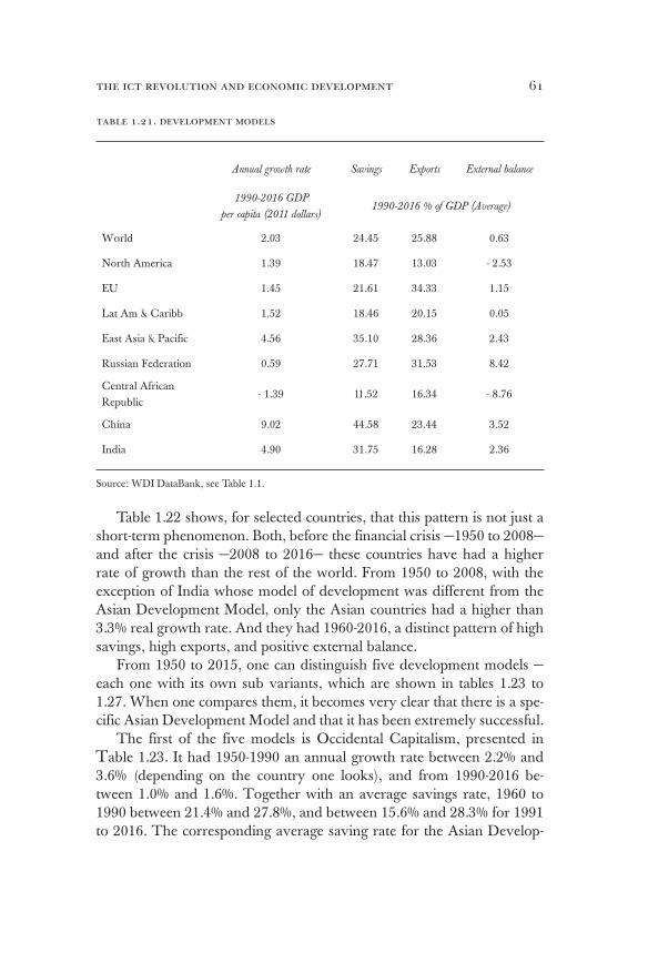
the ict revolution and economic development 61
table 1.21. development models
Annual growth rate Savings Exports External balance
1990-2016 GDP
per capita (2011 dollars)1990-2016 % of GDP (Average)
World 2.03 24.45 25.88 0.63
North America 1.39 18.47 13.03 - 2.53
EU 1.45 21.61 34.33 1.15
Lat Am & Caribb 1.52 18.46 20.15 0.05
East Asia & Pacific 4.56 35.10 28.36 2.43
Russian Federation 0.59 27.71 31.53 8.42
Central African Republic
- 1.39 11.52 16.34 - 8.76
China 9.02 44.58 23.44 3.52
India 4.90 31.75 16.28 2.36
Source: WDI DataBank, see Table 1.1.
Table 1.22 shows, for selected countries, that this pattern is not just a short-term phenomenon. Both, before the financial crisis —1950 to 2008— and after the crisis —2008 to 2016— these countries have had a higher rate of growth than the rest of the world. From 1950 to 2008, with the exception of India whose model of development was different from the Asian Development Model, only the Asian countries had a higher than 3.3% real growth rate. And they had 1960-2016, a distinct pattern of high savings, high exports, and positive external balance.
From 1950 to 2015, one can distinguish five development models —each one with its own sub variants, which are shown in tables 1.23 to 1.27. When one compares them, it becomes very clear that there is a spe-cific Asian Development Model and that it has been extremely successful.
The first of the five models is Occidental Capitalism, presented in Table 1.23. It had 1950-1990 an annual growth rate between 2.2% and 3.6% (depending on the country one looks), and from 1990-2016 be-tween 1.0% and 1.6%. Together with an average savings rate, 1960 to 1990 between 21.4% and 27.8%, and between 15.6% and 28.3% for 1991 to 2016. The corresponding average saving rate for the Asian Develop-
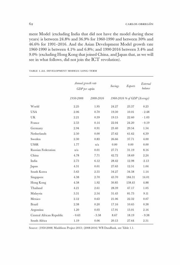
carlos obregón62
ment Model (excluding India that did not have the model during these years) is between 24.8% and 36.9% for 1960-1990 and between 30% and 46.6% for 1991–2016. And the Asian Development Model growth rate 1960-1990 is between 4.1% and 6.8%; and 1990-2016 between 3.4% and 9.0% (excluding Hong Kong that joined China, and Japan that, as we will see in what follows, did not join the ICT revolution).
table 1.22. development models: long-term
Annual growth rate
GDP per capitaSavings Exports
External
balance
1950-2008 2008-2016 1960-2016 % of GDP (Average)
World 2.25 1.95 24.27 23.37 0.23
USA 2.06 0.70 19.30 10.01 - 2.48
UK 2.21 0.39 19.15 22.60 - 1.03
France 2.53 0.14 22.04 24.20 - 0.19
Germany 2.94 0.91 23.40 29.54 1.54
Netherlands 2.50 0.00 27.62 61.62 6.39
Sweden 2.30 0.83 26.66 37.71 4.00
USSR 1.77 n/a 0.00 0.00 0.00
Russian Federation n/a 0.01 27.71 31.19 8.16
China 4.78 7.71 42.72 18.69 2.24
India 2.73 6.12 28.42 12.98 -2.13
Japan 4.31 0.01 27.63 12.51 1.04
South Korea 5.63 2.55 34.27 34.58 1.14
Singapore 4.38 2.70 43.70 184.31 14.01
Hong Kong 4.58 1.92 30.85 138.45 4.88
Thailand 4.21 2.61 28.39 47.17 1.05
Malaysia 3.31 2.54 31.43 81.73 9.11
Mexico 2.12 0.63 21.06 22.32 0.07
Brazil 2.38 0.20 17.16 10.65 0.38
Argentina 1.20 0.03 17.91 13.01 2.16
Central African Republic - 0.63 - 3.58 8.67 18.19 - 9.38
South Africa 1.19 0.06 20.13 27.64 2.51
Source: (1950-2008) Maddison Project 2013; (2008-2016) WB DataBank, see Table 1.1.
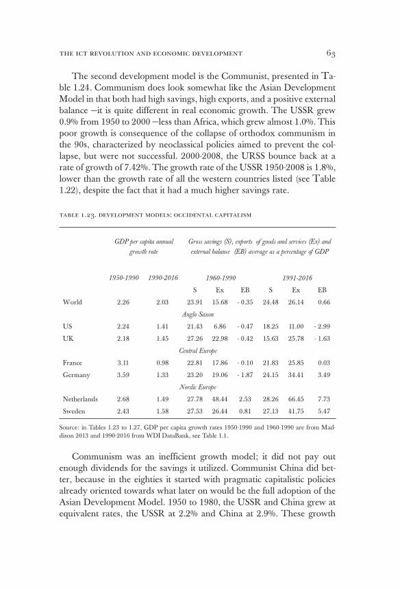
the ict revolution and economic development 63
The second development model is the Communist, presented in Ta-ble 1.24. Communism does look somewhat like the Asian Development Model in that both had high savings, high exports, and a positive external balance —it is quite different in real economic growth. The USSR grew 0.9% from 1950 to 2000 —less than Africa, which grew almost 1.0%. This poor growth is consequence of the collapse of orthodox communism in the 90s, characterized by neoclassical policies aimed to prevent the col-lapse, but were not successful. 2000-2008, the URSS bounce back at a rate of growth of 7.42%. The growth rate of the USSR 1950-2008 is 1.8%, lower than the growth rate of all the western countries listed (see Table 1.22), despite the fact that it had a much higher savings rate.
table 1.23. development models: occidental capitalism
GDP per capita annual
growth rate
Gross savings (S), exports of goods and services (Ex) and
external balance (EB) average as a percentage of GDP
1950-1990 1990-2016 1960-1990 1991-2016
S Ex EB S Ex EB
World 2.26 2.03 23.91 15.68 - 0.35 24.48 26.14 0.66
Anglo Saxon
US 2.24 1.41 21.43 6.86 - 0.47 18.25 11.00 - 2.99
UK 2.18 1.45 27.26 22.98 - 0.42 15.63 25.78 - 1.63
Central Europe
France 3.11 0.98 22.81 17.86 - 0.10 21.83 25.85 0.03
Germany 3.59 1.33 23.20 19.06 - 1.87 24.15 34.41 3.49
Nordic Europe
Netherlands 2.68 1.49 27.78 48.44 2.53 28.26 66.45 7.73
Sweden 2.43 1.58 27.53 26.44 0.81 27.13 41.75 5.47
Source: in Tables 1.23 to 1.27, GDP per capita growth rates 1950-1990 and 1960-1990 are from Mad-dison 2013 and 1990-2016 from WDI DataBank, see Table 1.1.
Communism was an inefficient growth model; it did not pay out enough dividends for the savings it utilized. Communist China did bet-ter, because in the eighties it started with pragmatic capitalistic policies already oriented towards what later on would be the full adoption of the Asian Development Model. 1950 to 1980, the USSR and China grew at equivalent rates, the USSR at 2.2% and China at 2.9%. These growth
carlos obregón64
rates were quite acceptable for international standards (Europe 12 larger countries grew 3.5%, the US 2.2%, and the World 2.6%). But they were obtained with large savings and huge internal investment that produced many structural inefficiencies, that ended up being one of the main causes of the collapse of the USSR.
China avoided the collapse becoming the first capitalist–communist country, by adopting the Asian Development Model and fully entering the ICT revolution. The difference in the economic models of the two mentioned nations can be seen easily. The Russian Federation adopted neoclassical policies 1990-2000 trying to prevent the collapse, conse-quence of many years of inefficiencies, and failed. Between 1990 to 2000, it had a negative annual growth rate of 3.77%.
In 2000, the Russian Federation produced only 0.65% of the GDP that was producing in 1990. As a consequence, between 1990 and 2016, the Russian Federation grew at an annual rate of only 0.6%, despite its savings rate of 27.7%; versus the 9.0% growth of China which had a much higher savings rate of 44.8%; or 5% growth of Thailand, which had a similar savings rates to the Russian Federation.
The third development model, presented in Table 1.25, is the Asian. As we had seen in Table 1.22, the Asian Development Model has clearly different features from other models since the 60s. Its long-term growth performance has been distinctly superior. However, nothing makes the unique characteristics of this model more transparent than analyzing its performance during the ICT revolution, 1990-2016. The first thing to note is that, with the ICT revolution, all the Asian countries listed in-creased significantly their savings as a percentage of their GDP (with the exception of Japan, which did not join the ICT revolution efficiently).
Thailand savings rate went from an average 24.8% in 1961-1990 to 30.2% in 1990-2015; Korea’s from 32.2 % to 35.1%; Malaysia from 26% to 34.4%; Singapore from 35.6% to 46.6%; China from 36.9% to 44.8%. India’s increase is from 21.8% to 31.9%. Hong Kong joined China, but maintained its high saving rate of around 30%. The increase in the saving rate of all these Asian countries is remarkable, especially since most other countries did not increase; the world’s saving average rate remained al-most unchanged between 1960-1990 and 1991-2016 (Table 1.23).
The second thing to note is that with the ICT revolution most of the countries that followed the Asian Development Model increased their ex-ports significantly. Average World exports over GDP increased 1.67 times (Table 1.23). Korea increased its exports over GDP 2.0 times; Hong Kong
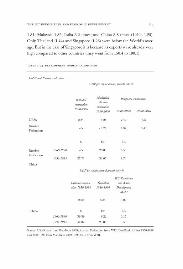
the ict revolution and economic development 65
1.81; Malaysia 1.82; India 3.2 times; and China 3.8 times (Table 1.25).
Only Thailand (1.44) and Singapore (1.26) were below the World’s aver-
age. But in the case of Singapore it is because its exports were already very
high compared to other countries (they went from 150.4 to 190.1).
table 1.24. development models: communism
USSR and Russian Federation
GDP per capita annual growth rate %
Orthodox
communism
1950-1990
Neoclassical
Western
communism
1990-2000
Pragmatic communism
2000-2008 2000-2016
URSS 2.24 - 4.26 7.42 n/a
Russian Federation
n/a - 3.77 6.92 3.41
S Ex EB
Russian Federation
1960-1990 n/a 20.03 0.55
1991-2015 27.71 32.05 8.74
China
GDP per capita annual growth rate %
Orthodox commu-
nism 1950-1980
Transition
1980-1990
ICT Revolution
and Asian
Development
Model
China
2.92 5.84 9.02
S Ex EB
1960-1990 36.89 6.22 0.15
1991-2015 44.82 23.80 3.53
Source: URSS data from Maddison 2009; Russian Federation from WDI DataBank; China 1950-1980
and 1980-1990 from Maddison 2009, 1990-2016 from WDI.
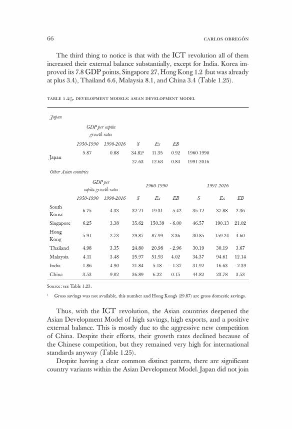
carlos obregón66
The third thing to notice is that with the ICT revolution all of them increased their external balance substantially, except for India. Korea im-proved its 7.8 GDP points, Singapore 27, Hong Kong 1.2 (but was already at plus 3.4), Thailand 6.6, Malaysia 8.1, and China 3.4 (Table 1.25).
table 1.25. development models: asian development model
Japan
GDP per capita
growth rates
1950-1990 1990-2016 S Ex EB
Japan5.87 0.88 34.821 11.35 0.92 1960-1990
27.63 12.63 0.84 1991-2016
Other Asian countries
GDP per
capita growth rates1960-1990 1991-2016
1950-1990 1990-2016 S Ex EB S Ex EB
South Korea
6.75 4.33 32.21 19.31 - 5.42 35.12 37.88 2.36
Singapore 6.25 3.38 35.62 150.39 - 6.00 46.57 190.13 21.02
Hong Kong
5.91 2.73 29.87 87.99 3.36 30.85 159.24 4.60
Thailand 4.98 3.35 24.80 20.98 - 2.96 30.19 30.19 3.67
Malaysia 4.11 3.48 25.97 51.93 4.02 34.37 94.61 12.14
India 1.86 4.90 21.84 5.18 - 1.37 31.92 16.63 - 2.39
China 3.53 9.02 36.89 6.22 0.15 44.82 23.78 3.53
Source: see Table 1.23.
1 Gross savings was not available, this number and Hong Kong´s (29.87) are gross domestic savings.
Thus, with the ICT revolution, the Asian countries deepened the Asian Development Model of high savings, high exports, and a positive external balance. This is mostly due to the aggressive new competition of China. Despite their efforts, their growth rates declined because of the Chinese competition, but they remained very high for international standards anyway (Table 1.25).
Despite having a clear common distinct pattern, there are significant country variants within the Asian Development Model. Japan did not join
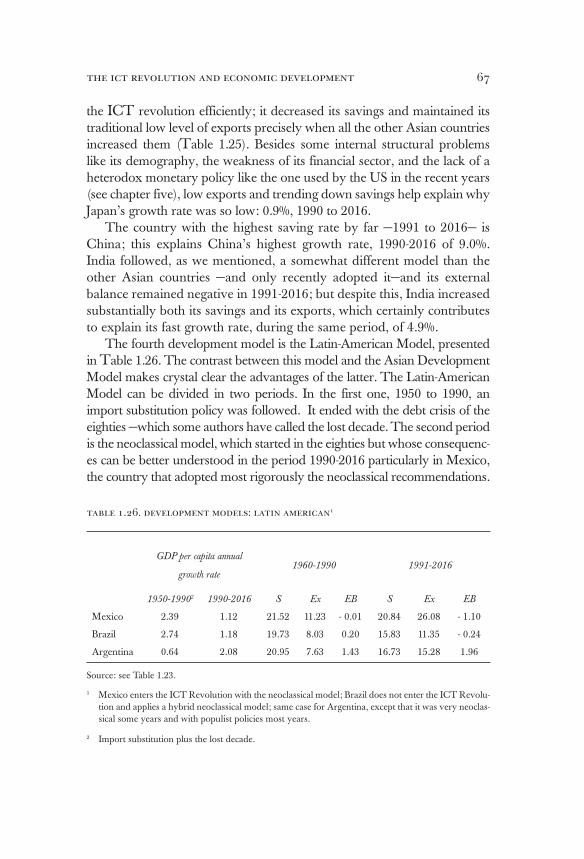
the ict revolution and economic development 67
the ICT revolution efficiently; it decreased its savings and maintained its traditional low level of exports precisely when all the other Asian countries increased them (Table 1.25). Besides some internal structural problems like its demography, the weakness of its financial sector, and the lack of a heterodox monetary policy like the one used by the US in the recent years (see chapter five), low exports and trending down savings help explain why Japan’s growth rate was so low: 0.9%, 1990 to 2016.
The country with the highest saving rate by far —1991 to 2016— is China; this explains China’s highest growth rate, 1990-2016 of 9.0%. India followed, as we mentioned, a somewhat different model than the other Asian countries —and only recently adopted it—and its external balance remained negative in 1991-2016; but despite this, India increased substantially both its savings and its exports, which certainly contributes to explain its fast growth rate, during the same period, of 4.9%.
The fourth development model is the Latin-American Model, presented in Table 1.26. The contrast between this model and the Asian Development Model makes crystal clear the advantages of the latter. The Latin-American Model can be divided in two periods. In the first one, 1950 to 1990, an import substitution policy was followed. It ended with the debt crisis of the eighties —which some authors have called the lost decade. The second period is the neoclassical model, which started in the eighties but whose consequenc-es can be better understood in the period 1990-2016 particularly in Mexico, the country that adopted most rigorously the neoclassical recommendations.
table 1.26. development models: latin american1
GDP per capita annual
growth rate1960-1990 1991-2016
1950-19902 1990-2016 S Ex EB S Ex EB
Mexico 2.39 1.12 21.52 11.23 - 0.01 20.84 26.08 - 1.10
Brazil 2.74 1.18 19.73 8.03 0.20 15.83 11.35 - 0.24
Argentina 0.64 2.08 20.95 7.63 1.43 16.73 15.28 1.96
Source: see Table 1.23.
1 Mexico enters the ICT Revolution with the neoclassical model; Brazil does not enter the ICT Revolu-tion and applies a hybrid neoclassical model; same case for Argentina, except that it was very neoclas-sical some years and with populist policies most years.
2 Import substitution plus the lost decade.
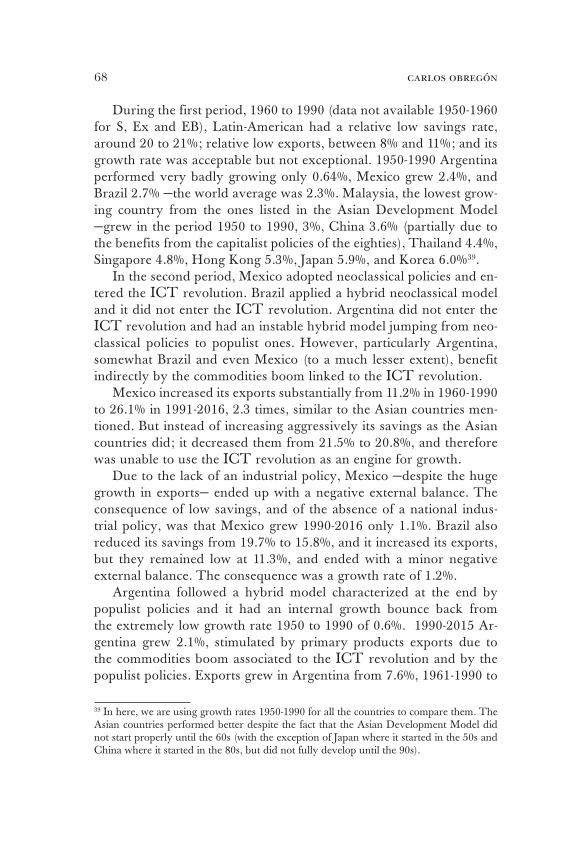
carlos obregón68
During the first period, 1960 to 1990 (data not available 1950-1960 for S, Ex and EB), Latin-American had a relative low savings rate, around 20 to 21%; relative low exports, between 8% and 11%; and its growth rate was acceptable but not exceptional. 1950-1990 Argentina performed very badly growing only 0.64%, Mexico grew 2.4%, and Brazil 2.7% —the world average was 2.3%. Malaysia, the lowest grow-ing country from the ones listed in the Asian Development Model —grew in the period 1950 to 1990, 3%, China 3.6% (partially due to the benefits from the capitalist policies of the eighties), Thailand 4.4%, Singapore 4.8%, Hong Kong 5.3%, Japan 5.9%, and Korea 6.0%39.
In the second period, Mexico adopted neoclassical policies and en-tered the ICT revolution. Brazil applied a hybrid neoclassical model and it did not enter the ICT revolution. Argentina did not enter the ICT revolution and had an instable hybrid model jumping from neo-classical policies to populist ones. However, particularly Argentina, somewhat Brazil and even Mexico (to a much lesser extent), benefit indirectly by the commodities boom linked to the ICT revolution.
Mexico increased its exports substantially from 11.2% in 1960-1990 to 26.1% in 1991-2016, 2.3 times, similar to the Asian countries men-tioned. But instead of increasing aggressively its savings as the Asian countries did; it decreased them from 21.5% to 20.8%, and therefore was unable to use the ICT revolution as an engine for growth.
Due to the lack of an industrial policy, Mexico —despite the huge growth in exports— ended up with a negative external balance. The consequence of low savings, and of the absence of a national indus-trial policy, was that Mexico grew 1990-2016 only 1.1%. Brazil also reduced its savings from 19.7% to 15.8%, and it increased its exports, but they remained low at 11.3%, and ended with a minor negative external balance. The consequence was a growth rate of 1.2%.
Argentina followed a hybrid model characterized at the end by populist policies and it had an internal growth bounce back from the extremely low growth rate 1950 to 1990 of 0.6%. 1990-2015 Ar-gentina grew 2.1%, stimulated by primary products exports due to the commodities boom associated to the ICT revolution and by the populist policies. Exports grew in Argentina from 7.6%, 1961-1990 to
39 In here, we are using growth rates 1950-1990 for all the countries to compare them. The Asian countries performed better despite the fact that the Asian Development Model did not start properly until the 60s (with the exception of Japan where it started in the 50s and China where it started in the 80s, but did not fully develop until the 90s).
the ict revolution and economic development 69
15.2% 1990-2016, which allowed this nation to have a positive exter-nal surplus of 2.0. However, Argentina did not enter the ICT revo-lution, did not improve its manufacturing production processes, and decreased its savings rate from 21%, 1960-1990, to 16.7%, 1990-2015. Therefore, it is clear that the Asian Development Model was quite distinct from the Latin-American Model, and that the second one was inferior in its economic performance.
table 1.27. development models: the hybrid african model
GDP per capita annual
growth rate 1960-1990 1991-2016
1950-1990 1990-2016 S Ex EB S Ex EB
Central African Republic
- 0.46 - 1.39 7.81 24.56 - 11.06 11.68 16.31 - 8.75
South Africa 1.04 0.83 25.37 27.05 3.30 16.69 27.22 0.98
Source: see Table 1.23.
The fifth and last development model is the hybrid African Model, which has so many variants that is almost impossible to define. Table 1.27 present two cases. The first case is the collapse of the Central African Republic that went down from a negative annual growth rate of 0.5% 1950-1990, to a negative 1.4% 1990-2016; as it decreased its exports and increased its savings, but they remained very low at 11.7%. The second case is South Africa, whose growth rate went down in the same periods from 1.0% to 0.8%, as it decreased its savings and main-tained its exports.
Now, we are finally in the position to fully answer the question that we made several pages before: why China? Japan was badly positioned because of its high wages, and the fact that the old institutions in Japan resisted the new technological change. China was well positioned and entered the ICT revolution with the correct new institutions. Thus, China can be explained as: ICT revolution + adoption of the Asian De-velopment Model. Mexico entered the ICT revolution with institutions belonging to old ideas —the neoclassical model— no longer relevant to the new technological conditions. That is why it did not grow.
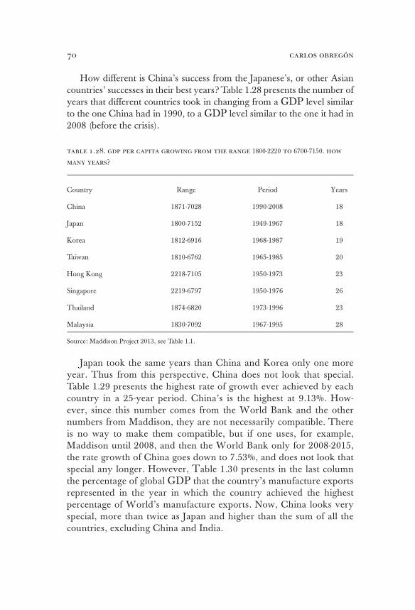
carlos obregón70
How different is China’s success from the Japanese’s, or other Asian countries’ successes in their best years? Table 1.28 presents the number of years that different countries took in changing from a GDP level similar to the one China had in 1990, to a GDP level similar to the one it had in 2008 (before the crisis).
table 1.28. gdp per capita growing from the range 1800-2220 to 6700-7150. how
many years?
Country Range Period Years
China 1871-7028 1990-2008 18
Japan 1800-7152 1949-1967 18
Korea 1812-6916 1968-1987 19
Taiwan 1810-6762 1965-1985 20
Hong Kong 2218-7105 1950-1973 23
Singapore 2219-6797 1950-1976 26
Thailand 1874-6820 1973-1996 23
Malaysia 1830-7092 1967-1995 28
Source: Maddison Project 2013, see Table 1.1.
Japan took the same years than China and Korea only one more year. Thus from this perspective, China does not look that special. Table 1.29 presents the highest rate of growth ever achieved by each country in a 25-year period. China’s is the highest at 9.13%. How-ever, since this number comes from the World Bank and the other numbers from Maddison, they are not necessarily compatible. There is no way to make them compatible, but if one uses, for example, Maddison until 2008, and then the World Bank only for 2008-2015, the rate growth of China goes down to 7.53%, and does not look that special any longer. However, Table 1.30 presents in the last column the percentage of global GDP that the country’s manufacture exports represented in the year in which the country achieved the highest percentage of World’s manufacture exports. Now, China looks very special, more than twice as Japan and higher than the sum of all the countries, excluding China and India.
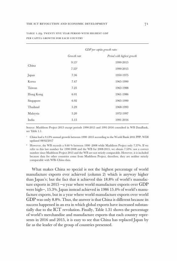
the ict revolution and economic development 71
table 1.29. twenty five year period with highest gdp
per capita growth for each country
GDP per capita growth rates
Growth rate Period with highest growth
China 9.131 1990-2015
7.532 1990-2015
Japan 7.36 1950-1975
Korea 7.47 1965-1990
Taiwan 7.25 1963-1988
Hong Kong 6.01 1961-1986
Singapore 6.92 1965-1990
Thailand 5.29 1968-1993
Malaysia 5.20 1972-1997
India 5.15 1991-2016
Source: Maddison Project 2013 except periods 1990-2015 and 1991-2016 consulted in WB DataBank, see Table 1.1.
1 China had a 9.13% annual growth between 1990 -2015 according to the World Bank 2011 PPP. WDI updated 08/02/2017
2 However, the WB records a 9.60 % between 1990 -2008 while Maddison Project only 7.37%. If we refer to this last number for 1990-2008 and the WB for 2008-2015, we obtain 7.53%: not a correct number since Maddison Project 2013 and the WB are not strictly comparable. However, it is included because data for other countries come from Maddison Project, therefore, they are neither strictly comparable with WB´s China data.
What makes China so special is not the highest percentage of world manufacture exports ever achieved (column 2) which is anyway higher than Japan’s; but the fact that it achieved this 18.8% of world’s manufac-ture exports in 2015 —a year where world manufacture exports over GDP were high—, 15.3%. Japan instead achieved in 1986 15.4% of world’s manu-facture exports, but in a year where world manufacture exports over world GDP was only 8.8%. Thus, the answer is that China is different because its success happened in an era in which global exports have increased substan-tially due to the ICT revolution. Finally, Table 1.31 shows the percentage of world’s merchandise and manufacture exports that each country repre-sents in 2016 and 2015, it is easy to see that China has replaced Japan by far as the leader of the group of countries presented.

carlos obregón72
table 1.30. highest share of world´s exports ever achieved (1960-2016)
Year
1. Highest %
of world´s mer-
chandise exports
ever achieved
2. Highest %
of world´s
manufacture
exports ever
achieved
3. World´s manu-
facture exports as
a % of World´s
GDP
in year, cor-
responding
to column 2
4.- Country´s
manufacture
exports as a
% of world´s
GDP in year,
corresponding to
column 2
China 2015 13.71 18.80 15.33 2.80
Japan 1986 10.12 15.37 8.82 1.36
Korea 2015 3.18 4.14 15.33 0.63
Hong Kong 1993 3.52 4.57 10.73 0.49
Japan & Korea 1986 11.78 17.77 8.82 1.57
Hong Kong & China
2015 16.80 21.72 15.33 3.33
Singapore 1996 2.29 2.65 12.48 0.33
Thailand (year) (2016) 1.34 (2015) 1.46 (2015) 15.33 0.22
Malaysia 2000 1.51 1.71 13.80 0.24
India (year) (2014) 1.69 (2015) 1.65 (2015) 15.33 0.25
∑ (except China + India)
(year) (1994) 19.38 (1993) 24.09 (1993) 10.73 2.58
∑ (year) (2015) 29.93 (2015) 37.29 (2015) 15.33 (2016) 5.71
Source: WDI DataBank, see Table 1.1.
There have been many explanations as to why Japanese growth had been so low for so many years. Many factors can be mentioned, such as its demographic transition to an old population, its financial crisis, and the fact that the Japanese Central Bank monetary policy was never ag-gressive enough —as Bernanke’s, the aggressive commercial policy of the Clinton administration or the transition to a true democracy— when the one party that had been in power for 50 years lost the elections. All these factors may have been of influence, and they may explain, to some ex-tent, why Japan grew only 0.9% 1990 to 2016 versus North America 1.4%,
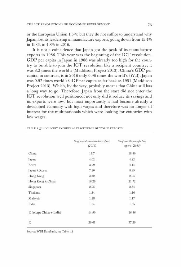
the ict revolution and economic development 73
or the European Union 1.5%; but they do not suffice to understand why Japan lost its leadership in manufacture exports, going down from 15.4% in 1986, to 4.8% in 2016.
It is not a coincidence that Japan got the peak of its manufacture exports in 1986. This year was the beginning of the ICT revolution. GDP per capita in Japan in 1986 was already too high for the coun-try to be able to join the ICT revolution like a recipient country; it was 3.2 times the world’s (Maddison Project 2013). China’s GDP per capita, in contrast, is in 2016 only 0.96 times the world’s (WB). Japan was 0.97 times world’s GDP per capita as far back as 1951 (Maddison Project 2013). Which, by the way, probably means that China still has a long way to go. Therefore, Japan from the start did not enter the ICT revolution well positioned: not only did it reduce its savings and its exports were low; but most importantly it had become already a developed economy with high wages and therefore was no longer of interest for the multinationals which were looking for countries with low wages.
table 1.31. country exports as percentage of world exports
% of world´s merchandise exports
(2016)
% of world´s manufacture
exports (2015)
China 13.7 18.80
Japan 4.02 4.82
Korea 3.09 4.14
Japan & Korea 7.10 8.95
Hong Kong 3.22 2.94
Hong Kong & China 16.29 21.72
Singapore 2.05 2.34
Thailand 1.34 1.46
Malaysia 1.18 1.17
India 1.64 1.65
∑ (except China + India) 14.90 16.86
∑ 29.61 37.29
Source: WDI DataBank, see Table 1.1
carlos obregón74
Japan entered the ICT revolution like the developed economy that it is: like an investor. And as an investor, it was also not very well po-sitioned. Due to its history of producing large part of its manufacturing production locally, Japan as late as 2005 only had an outward foreign direct investment (FDI) equivalent to 8.46% of its GDP compared with 27.78% for USA, or 34.56% for the EU (Table 1.5). Of course, this was not enough for Japan to recover its normal growth or to maintain its lead-ership in manufacture exports. Since 2005, Japan has started a great effort to increase its foreign investments to join the ICT revolution, for 2015 its outward FDI was already 29.7% of GDP, but still lower than USA’s 33.3%, Germany’s 40.93%, UK’s 54.46%, or EU’s 59.84%.
We can distinguish three different technological eras. The first one was the computers chips revolution in which Japan was very successful. The second one is the one we are living, the ICT revolution in which China is being very successful. And the third one, which to some extent seems to be already starting, maybe automation of production with the increased use of robots capable of performing more tasks and to take more decisions. Will automation mature into a new technological revolu-tion? We do not know. But it is a good bet: if it does, its implications will be huge for the global economy.
the sources of growth
There have been several generations of economic growth models trying to explain: what produces economic growth? They are part of the general economic thinking that defines the three generations of economic devel-opment theories40. The first generation of theories was built in the spirit of Keynesianism. The growth model that dominated this generation was Solow’s —the laureate Nobel Prize winner. In this model, technology is exogenous, and the long-term Stationary State (sustainable) growth —as-suming a given technology— is given by the rate of population growth.
An exogenous positive technological shock increases the long-term per capita product. Short-term growth depends on the savings rate; it moves the economy from one growth path to another. If an economy
40 A good summary of the diverse economic growth models in the literature and its impli-cations for the three generations of economic development theories is found in Obregon 2008a.
the ict revolution and economic development 75
increases its saving rate, it will move from a Stationary State with less per capita product to another with more per capita product. Solow’s model, in the spirit of the Keynesian models, suggest a role for the government: to increase savings. The policy recommendation was clear; an economy must increase its saving rate as much as possible until it reaches the maxi-mum possible consumption per capita —which was called the golden rule.
An interesting feature in this model is that savings are always equal to productive investment —investment that produces with the given tech-nology— which implicitly is the best available in the frontier. The notion that savings are always productive is inherited from classic and neoclas-sical economists, and in fact, if we are only concerned with the history of western economic development, it is a good assumption because by definition the technology used is at the frontier —the West includes the most advanced economies of its time. This assumption, however, is not optimal to understand the economic history of less developed economies. The failure of the USSR was precisely that it did not produce with the frontier technology, which was the one used by the West. It was also a problem with the import substitution model, which focused only in the saving rate and not in the quality of the technology used.
The second generation of economic development theories was built in the spirit of the Keynesianism’s demise and the triumph of Monetar-ism and Neoclassical Economics. The main idea was to explain economic growth as endogenous, as consequence of the markets without govern-ment intervention. If capital moves freely between one country and the next, and with global technology given and defining the same growth path for all the countries, given diminishing returns one should expect economic convergence between all the countries of the world —as capital moves to those countries with higher returns, given their relative labor abundance.
Empirically, absolute convergence does happen between developed economies (and within regions in a given develop economy), but not with developing economies (with the exception of a selected group of Asian economies). Endogenous human capital models were built to ex-plain why. The reason given by these models (by Lucas, the Nobel Prize winner) was that developing countries do not have the quality of labor required41. This of course does not explain why the good quality labor does not migrate to the developing countries, if theoretically it could get higher remuneration there —because it will be more productive due to
41 Lucas 1988.
carlos obregón76
the available low-quality labor. Moreover, empirical studies have shown that the years of schooling only explains around 25% of the difference in per per capita GDP. And since only 16% is explain by fixed capital, then around 60% must be explained by institutional differences42.
Lucas’ response to this empirical reality was to argue that human capital is not only education, that there is something that he calls social human capital, which enriches the productivity of a given worker in de-veloped countries. However, if to calculate this human social capital one uses the difference of migrant’s salaries versus their own countries, we still only explain 33% of the previously mentioned difference. Therefore, still 50% is explained by institutional differences43.
Finally, Lucas argued that the Asian countries development must be understood as an increase in human capital through learning-by-doing, due the production of international competitive goods. But then, how do we measure labor? Lucas’ response is that through its value added —us-ing international prices, but this is a tautological definition. Lucas ended where Marx did, because if labor quantity (or quality) is to be defined by the market value added, then really there is no way to measure labor ex ante —and to argue that labor is the cause of the value added by which it is measure is a tautology of not much significance.
The Asian economic growth is explained by the Asian Development Model, and there is no sense in arguing that it is due to more human capital. It happened in Korea, which started with much less human capi-tal than Philippines. The problem with human capital in the second gen-eration is exactly the same as with savings in the first generation: ex ante we do not know if they are going to be productive or not. In the case of physical capital, it depends upon whether it uses or not the technology at the frontier, and the same happens with human capital.
It is not education in general what counts: Argentina, Eastern Europe, and Russia had it, and they did not grow; Korea or Singapore did not have it, and did grow. What counts is labor training related to the frontier technology. What counts is the technology at the frontier, be it for physi-cal or human capital, and this signals the importance of exporting to the developed economies’ middle class.
As the third generation of economist has explicitly acknowledged, there is no way out of the fact that the divergence or convergence of a given developing country towards the developed economies depends 42 Hall and Jones 1999.
43 Klenow and Rodriguez – Clare 1997.

the ict revolution and economic development 77
upon its institutional characteristics. Hall and Jones have shown that the social infrastructure is an important element to explain economic growth44. They define social infrastructure as the institutional arrange-ment that promotes production and investment, instead of consumption and enjoyment. Countries with otherwise similar cultures like South Ko-rea and North Korea, communist China under Mao versus Taiwan or Hong Kong, East Germany versus West Germany —show huge GDP differences that are in the 2.5 to 10 times range45.
Institutional models have been very useful to show the importance of the institutional differences among countries, but in general, have been bias towards arguing that what causes development is to adapt and rede-sign the local institutions so that they resemble the western institutions. Since worldwide regressions always involved the West, and it has great weight on them due the size of its GDP, it is no surprise that the Western institutions ended up correlating well with economic growth.
One of the institutional features argued by the third generation, as required for economic growth, is democracy. Most of Asia developed being non-democratic, but then many countries did become democratic; therefore, there is ground for discussion. But China not only is not demo-cratic, it is communist —and who can deny its success. The undeniable fact is that the only countries that had been successful to converge are a selected group of Asian countries —which construed a specific insti-tutional arrangement that does not resemble the West institutions. Not only they did not follow the recommendations of the western economists, they based their success in an alternative: the Asian Development Model.
In Solow’s model, per capita economic growth without technological change tends to zero. Therefore, it was necessary to explain: why does technology change? Endogenous growth models offered four explana-tions: 1) science; 2) talented individuals; 3) learning by doing; and 4) firms’ research and development46. All of these explanations are very use-ful to understand: why per capita GDP has grown so fast in capitalism? The benefit of science for mankind is undeniable, and it has everything to do with the long-term capitalism growth, but from that does not follow
44 Hall and Jones 1999.
45 Olson 1996.
46 Science: Phelps 1966, Nordhaus 1967, Shell 1966 and 1967. Talented individuals: Baumol 1990 and Murphy, Shleifer, and Vishny 1991. Learning by doing: Arrow 1962. Research and development: P. M. Romer 1990, Grossman and Helpman 1991, Aghion and Hewitt 1992, D. Romer 2001.
carlos obregón78
that investing in science will produce economic growth in a given coun-try, as the USSR learned the hard way.
Moreover, scientific discoveries always existed, and the critical ques-tions is: why did they accelerate as much in Capitalism? North argues that innovation of free individuals is the key, and to a large extent he is right. However, as Veblen pointed out, science and technology are, for the first time in Capitalism, so closely intertwined that they foster each other developments. And technology, as Smith taught us, is related to the size of the market (mainly defined by two factors: global trade and the size of the middle class). Research and development precisely shows the power of the interconnection between science, technology, and market size.
Models of research and development explain convergence through technological transfer47, but human capital differences and particularly institutional asymmetries make such transfer difficult. The ICT revolu-tion made it easier.
The importance of talented entrepreneurs versus rental seekers is undeni-able, but it happens in different ways in diverse societies. Old societies were not exempt of these individuals, and they did not grow fast. These indi-viduals operate in Japan in groups, while they do it individually in the West. The same happens with learning-by-doing: its relevance is undeniable, but it happens in all societies and historical times. What is important is learning-by-doing at the technological frontier, to have talented individuals at that fron-tier, and to have science, technology, firm’s research and development, and markets interconnected —all of this was key in the development of the West.
The Asian Development Model implied learning from the West —through exporting sophisticated goods to the middle class of developed economies. The unique feature of the ICT revolution is that it made easier the transfer of such knowledge, because it allowed for manufactur-ing service centers in the developed world to be able to coordinate manu-facturing production chains offshore. This implies that neither the labor has to migrate to the rich countries, nor sophisticated human capital has to migrate to developing economies.
Physical capital migrates and technology is transferred, but under conditions defined to some extent by the service centers. The countries that were able to learn and to receive adequate technological transfers were those who saved to promote their internal growth; those whose sav-ings allowed them to develop an industrial policy of their own to promote world competitive national companies. Let us discuss briefly what are, in
47 Jaumott 1999, Caselli and Colman 2001.

the ict revolution and economic development 79
general, the growth sources for a given economy. There are three sources of growth: 1) The value added in exports; 2) the substitution of imports; and 3) the growth of internal productive chains, of which a classic exam-ple could be construction, but there are many others including services and primary products. The first thing to understand is that value creation through GDP growth is not necessarily permanent. Take the case of East Germany that had been growing at very high rates before it joined in with West Germany. Before they came together, it was argued that the two Germanys were extremely productive because of the German character. When East Germany joined in, it represented around 13% of West Germany’s GDP; five years later, it was in the vicinity of 8%48. Why? Because most of the goods and services offered by East Germany were not competitive by western standards. The same happened with the USSR when it opened up in 1990. By 2000 it was producing only 65% of the total GDP that it was producing in 199049.
Therefore, the problem is that if an economy closes itself it may be growing fast, but when it opens up to the world, it may be worth very little —because as soon as foreign competitors arrive and make the tech-nology used obsolete, a lot of the old economy’s value disappears. In a competitive international world, value added growth has to be associated with technology at the frontier, at least for significant segments of the economy —that is why exporting to developed economies is so crucial. Later on, other segments of the economy may transform themselves as they get linked more efficiently to the exporting segments.
The difference between the USSR and the successful Asian Develop-ment Model, is that the latest was guided by the dynamic preferences of the middle class in the developed nations, and therefore was always learning technology in the frontier. The USSR invested a lot in science and technol-ogy, but was not successful because it did not have a dynamic market guid-ed by the dynamic preferences of the the middle class mass consumption. The fundamental problem of the communist development model is that it did not participate in world markets; it did have a large domestic market, but the market did not have a broad middle class. The USSR model was driven by military and space spending, and was trying to copy the Western capitalist model; it had high levels of savings, scientific development, and high levels of education, but it did not have the most important element: mass production technology aimed at a middle class.48 See Obregon 1997, p 260 and Smyser 1993, chapters 7 and 8.
49 Calculated with Maddison 2009.
carlos obregón80
The import substitution model has the same faults than the commu-nist model. The consequence of not participating in the developed coun-tries world-class market was that Latin American technology became ob-solete. Pretending to substitute imports of durable consumer goods, and especially capital goods, by definition meant the use of obsolete technol-ogy, given the size of the local market.
The problem with economies whose development is based upon “closing the economy” is that they do not resist the pressure of the in-ternational competition when they open up. Behind the disastrous per-formance of the 1990-2000 USSR —when the neoclassical policies were implemented— was the incapacity of the old industrial plant to face global competition. The poor performance of Latin America in the lost decade of 1980-1990 and afterwards, was not only due to the debt crisis of the 80s. It was also caused by the fact that large part of the industrial plan, built during the years of the import substitution model, was slowly but certainly eroding its economic value due to its incapacity to compete in the global market.
Brazil and Argentina did not join the ICT revolution, and their indus-try technology is obsolete. Mexico did join the ICT revolution, and large part of its export industry has been modernized, consequently. But be-cause of the lack of adequate savings, Mexico has been unable to transfer efficiently this modernization to the rest of the economy, and to promote satisfactory economic growth.
The Asian Development Model is a dependent model in the sense that it is guided by exports to the developed economies. But, it also uses the import substitution strategy —as all of these countries found ways to restrict their imports. Creating a positive trade balance allowed them to have control over their long-term investment and industrial strategy. Their industrial strategy was not dictated by the bureaucrats like in the USSR. The Jetro, created by the MITI in Japan, and the Kotra in Korea, were formed with the participation of the private sector50. Planning was flexible and always ready to be judged by market success, particularly in exports. In Japan, the computer chip industry was a success story leaded by the bureaucrats; the automobile industry was a success story opposed by the bureaucrats, but that the private sector could implement anyway.
50 Kotra and Jetro are associations of foreign trade. The Jetro was instaurated by the MITI in charge of industrial and trade planning in Japan, and the Kotra by the ministry of in-dustry and commerce in Korea —which performed similar tasks to the MITI in Japan. See Obregon 1997, p 304.

the ict revolution and economic development 81
The Asian Development Model is based in huge national savings use for three purposes: 1) Finance a fast growth of internal value chains pro-tected from the competition either by disguised mercantilist policies, or by the exchange rate, or most often a combination of both. 2) Finance a growing interconnection of the internal value chains with the export seg-ments to increase the dissemination of knowledge. 3) Finance a growing exporting national industry, concentrated mainly in manufactures.
The Asian Development Model is distinct in each country, but has some elements in common51:
1. A powerful regulatory state that guides the model. 2. Flexible planning involving the private sector, with a high de-
gree of autonomy for companies. 3. The private sector establishes clear commitments, and it is of
paramount importance in the definition of the model. 4. The model is based on exports; production is oriented to com-
pete in the global market.5. High internal savings.6. Cutting-edge foreign technology. 7. A learning process that promotes local technology and com-
petitiveness with the outside world.8. Exports are the basic axis of the model, but at the same time it
efficiently defends the growth of the domestic market, through: a) a series of regulations that —without being tariffs— hinders the growth of imports, and b) through an undervalued exchange rate.
9. A national agreement that reinforces the historical social be-longing of each nation through the commitment to unite to compete with the outside world. The agreement is for econom-ic growth, in the understanding that the only way to achieve this is by competing head to head with the developed world, that is why is so important to export to it.
10. In all cases, there is awareness that it is necessary to learn from the West and negotiate with the West, but always with the aim of competing with it.
11. In all cases, the competitive model strengthened and used tra-ditional local institutions, while creating new ones oriented to global competition.
12. The central objective is to guarantee economic growth at the national level.
51 (Obregon 1997, 2008c)
carlos obregón82
China had seen the success of the Asian Development Model in other countries, and adopted it to take advantage of its extraordinary position versus the ICT revolution. This was the Key to its success.
conclusion
The key to economic growth is technological innovation, which requires two conditions: a large market and massive consumption. All human kind empires were developed based on increasing the market size, but their problem was always that the empire’s costs of the military and bu-reaucratic administration grew exponentially as it expanded, and the provinces were increasingly more distant from the imperial center. The empires of the past grew on the basis of new markets conquests and of adding wealth to the empire, but lacked an internal motor of growth. What distinguishes capitalism from previous productive models is that it is based on the expansion of the middle class mass consumption. That provides an engine of internal growth.
It is the middle class that rebels against the upper class in Europe. It is the one that changes the productive model’s conditions of consumption; with this begins the great economic expansion that characterizes capital-ism. What was it that changed? Massive production–aimed at meeting the needs of the growing middle class–allowed a brutal expansion in tech-nological development. It is not possible to innovate if a handicraft des-tinated to kings is to be produced by hand, but it is possible to innovate when large-scale consumer goods are produced.
The relationship between the mass consumption of the middle class and technological development has been, however, traditionally underes-timated by the main western schools of economic development.
There are three generations of economic development theories. The first one, guided by Solow’s economic growth model, identifies savings as a source of growth. And to a large extent it was right, because, as Paul Samuelson once told me, “Solow’s model might be wrong in several dimensions, but what remains true is that there is no economic devel-opment without savings”. Savings were a central element of the import substitution policies, which sought for developing economies to save as much as the West did. It was also central in the communist strategy for development, particularly in the USSR, which was trying to obtain eco-
the ict revolution and economic development 83
nomic growth the way the West had done it. But savings, as history has shown us. while required do not suffice.
The Asian Development Model has recognized that saving is crucial, and in fact, it has shown that it is needed to save substantially more than what the West did. However, it has also shown that savings are not enough. Savings have to be oriented to good investments with high inter-national competitive technology —here is where the middle class becomes crucial. A savings strategy must be joined by an exports strategy oriented towards the developed economies’ middle class, so that the investments are guided by the proper technology.
The second generation of economists describe the lack of success of the first generation as due to large bureaucratic governments, the absence of free prices, and the lack of free trade. Based upon this analysis and in the neoclassical model, this second generation of economists argued that if the proper economic policies are followed, capital will flow from the de-veloped to the underdeveloped economies, and development will occur. In real life, it did not happen because of the institutional constrains that characterize the underdeveloped economies, such as the social political and legal framework, lack of infrastructure, slow administrative proce-dures, and so on.
The third generation understood the limitations of the second, and recognized the relevance of institutional factors. But still, it insisted in seeing development as the consequence of the adoption by underdevel-oped economies of the right institutions —identified practically in all the authors as the institutions that characterized the West52.
The Asian Development Model provided in the real world a new ex-planation for development, one that was not foreseen by the theorist of economic development. It was based in high savings —like the first genera-tion—, in orienting the economy towards trade —like the second genera-tion—, and it recognized the relevance of the institutional arrangement–like the third generation; but it added three new surprising elements.
First, a new institutional arrangement was implemented, but it did not copy the West’s. Second, it recognized the need to integrate the economy to the global market —like the second generation—, but it did it primor-dially through promoting exports and restricting imports —like the first generation. And third, like the first generation, it recognized the need of high savings, but it introduced the innovation of savings much higher than the West’s. In a very surprising conclusion, imposed upon us by
52 For a detailed decription of the three generations of economists, see Obregon 2008a.

carlos obregón84
economic reality, we learned with the Asian Development Model that de-velopment happens when the poor save for the rich to consume, and not like previous theory told us, when the rich save to lend to the poor —for the latter to have capital to develop.
In this chapter, we have provided a historical perspective that offers two lessons. First, technological revolutions always deeply change human societies. Second, institutions are not always ready to accept the implica-tions of the new coming technology; and when they resist, it ends up being very damaging for the economic development of those countries involved. Technological revolutions changed the global economic land-scape, and when they are abrupt institutions do not have enough time to adjust themselves; the old ideas and institutional arrangements are unable to change fast enough.
With the advent of the ICT revolution: Japan did not change, it con-tinued with its same old strategies, it lost its primacy, and had nil eco-nomic growth; Mexico applied the old neoclassical ideas and did not develop; China, in instead, understood the opportunity and created new institutional arrangements to host the new investors, under the umbrella provided by the adoption of the Asian Development Model, and was very successful.
An important conclusion of this chapter is that the ICT revolution of-fers the opportunity of a sustained long-term global productivity increase, and that the world must reap its benefits. Trying to prevent the ICT rev-olution from happening —through nationalism and protectionism— will not work; it will occur any how, but a lot of unnecessary damage would be produced to the global economy in the process of pretending to stop it.
We have explained that the ICT revolution allowed for the fragmen-tation of production, and we have shown that the ICT plus the Asian Development Model explains the success of China. The ICT revolution also explains the success of India, but this country followed its own devel-opment model —basically based in offshore services. Japan’s wages were already too high, and the beginning of the ICT revolution signaled the end of the Japan’s primacy. While Japan decreased its savings and main-tained its exports over GDP low, most other Asian countries increased their savings and their exports to face the opportunity, and the increasing competition that the ICT revolution and China meant. These countries performed much better than Japan.
Mexico entered the ICT revolution, while other Latin American countries did not, although they benefited indirectly through the com-
the ict revolution and economic development 85
modities boom. Mexico, however, decreased its savings and did not have an industrial strategy; therefore, despite joining the ICT revolution, it did not grow. The ICT plus the Asian Development Model was a suc-cess story for the Asian countries; the ICT plus the neoclassical model was a story of failure for Mexico.
We have noted the relationship between the anti-migration policies and the ICT revolution. As the firms go offshore, they are no longer interested in promoting migration; therefore, the anti-migration groups no longer have opposition.
In this chapter, we have reviewed the way the ICT revolution ex-plains:
1. The high global economic growth 1990-2008 and why it has remained relatively high, even after the crisis.
2. The fragmenting of manufacturing production in offshore lo-cations.
3. That economic competition is no longer between nations or sectors, but between stages of production.
4. The fast increase of world’s FDI. 5. The rapid increase of world’s manufacture and merchandise
exports over world’s GDP. 6. The fast growth of China and India. 7. The demise of Japan. 8. The low growth of Mexico. 9. The anti-migration policies. Many other critical consequences of the ICT revolution will be ad-
dressed in the following chapters.
[86]
NATIONALISM AND CHANGES
IN THE INCOME DISTRIBUTION
The most surprising event in today’s global economy is the revival of nationalism, protectionism, and anti-migration policies. These three phe-nomena were thought by many as events of the past. The lessons of the two wars, Bretton Woods, The IMF, The World Bank, and the World Trade Organization, particularly the last, seemed to many that had her-alded the triumph of globalization over nationalism and protectionism. The European Union was thought as an initial experiment indicative of what future globalization might look like. But all these optimistic views turned out to be wrong. Not only globalization is not advancing, but lately it seems that it is going backwards. Thus, the inevitable question is: why?
An explanation offered by many authors is that the deterioration in the developed countries’ income distribution, consequence, they say. of the avarice and unsatisfying ambition of the high class, has brought a lot of social discontent53. These authors argue that the middle class has real-ized that “China–large West companies deals” are not in its benefit. We will argue that this view is incorrect.
The concentration of income in the developed economies is not the outcome of class conflict —the abuse of the high class. It is the conse-quence of the fundamental transformations that the ICT revolution has brought about, and the incapacity of the old ideas and institutional ar-rangements to adapt to the new circumstances. We will show that not all the countries responded the same way, and that some institutional arrangements were more resilient than others to the new international mode of production income distribution pressures.
Moreover, we will propose that today’s anger and political disgust of the middle class in the developed countries is a direct consequence of the 2008 crisis, and not of the deterioration of the income distribution. Changes in the income distribution have happened often in history, due to all kind of exogenous shocks, and the way societies accommodate to
53 Piketty 2014, Piketty article in The Guardian 2016, Bourguignon 2016. P VIII.
nationalism and changes in the income distribution 87
them. They happen, most of the times, without the huge social discon-tent that we have been observing lately.
The argument that Chinese exports and the avarice of the rich had damaged the loosely defined middle class in developed economies has been defended by prestigious economists. They have made it popu-lar. The middle class has learned from them. But in reality, the angriness of the middle class is explained by the 2008 financial crisis. A crisis that did not have to happen, and that had nothing to do with the avarice of the rich or with China’s exports.
Chinese exports did damage the income of some sectors of the middle class in developed economies —those employed in manufacturing produc-tion. But three considerations are needed:
1. Independently of the benefits that the ICT revolution has brought to the high class —the top ten percent owning real estate and stocks— all of the middle class in the developed economies benefited from the higher Chinese exports. These meant:
a) Lower prices. b) Lower inflation expectations, and therefore lower nominal
long-term interest rates. c) Lower long-term real interest rates —due to an increase in
global savings. d) b) + c) meant accessible credit at low long-term interest
rates. e) Higher economic growth, and therefore higher employ-
ment growth. Consequently, 2. Each one of the developed economies —as a nation— benefited
from the higher Chinese exports; thus, it ends up being a redis-tribution problem inside each one of these countries.
Moreover,3. The Chinese phenomenon improved the global income distri-
bution.We will show that despite the fact that there has been an income
distribution deterioration in the developed economies, it is not likely that this was what initiated the social discontent that we have been observing. People are angry at the system, not because the relative distribution of income has worsened; but, by its inability to offer economic growth and progress. The income distribution deterioration in the USA and the UK happened before 2008, and in 2008 we did not have the social angriness
carlos obregón88
that we witness today. The main cause of today’s social disgust is the 2008 financial crisis, which produced massive losses of assets, high levels of unemployment and the stagnation of the economy.
The official explanation of the 2008 crisis states that global over sav-ing, consequence of China’s, Germany’s, and others’ exports, brought the real interest rate down and provoked the real state boom —whose inevitable crash was the cause of the 2008 crisis. And it is argued that the crisis was as big as it was because of the high classes’ greediness repre-sented by financial institutions among others. In the next chapter we will show that the official explanation is incorrect.
The 2008 crisis did not have to happen. It was consequence of the incapacity of institutions and ideas to adapt to the new reality brought by the ICT revolution. Due to the success of Bretton Woods, the world forgot that economic growth and stability were not just the result of free markets —but, that the proper institutional arrangement was needed. As the free market ideology expands, the main regulators distant themselves from the markets under the belief that these could auto-regulate them-selves. And, consequently, they did not fulfill their duty to provide the markets with the proper institutional arrangement.
There have been many recent developments, both in economic theo-ry and in economic reality, that have clearly shown that institutions are required to be able to attain a proper economic equilibrium.
As to the theory:1. The demise of welfare economics due to Arrow’s theorem and
its reconstruction by Sen, who introduced value judgments —which are nothing else than conceptual systems, i.e. institutions.
2. Stiglitz informational theory that produces multiequilibria.3. Nash non-paretian (suboptimal) multi equilibriums. 4. The resurgence of institutional economics, North and others.As to the reality:1. The 2008 crisis showed that the theory of rational expectations
was lacking something very crucial in the understanding of economic reality.
2. The failure of the neoclassical theory of economic develop-ment, both in the former USSR and in Latin America —with Mexico being the clearest example, because its strictly adher-ence to the neoclassical model.
But despite of so many evidence, both theoretical and empirical, the old free market ideology has subsisted, and still dominates most local and
nationalism and changes in the income distribution 89
global policy recommendations. We will show in the next chapter that the 2008 crisis was a consequence of the free market ideology’s incapacity to adapt to the new world brought about by the ICT revolution.
People got angry at the system due to assets losses, unemployment, and lack of economic growth, consequence of the 2008 crisis. Also, economists blamed the 2008 crisis and the deterioration of the income distribution on: China’s exports and the wealthiest greediness. Therefore, people believe it. And as a consequence it became popular for politicians to defend national-ism, protectionism, and to support anti-migration proposals:
1. Defend protectionism: policies to force other countries, mainly China, to reduce their external surplus.
2. Defend nationalism: the interest of the rich being linked to ex-ternal interests is argued to be opposed to the interest of the majority–the idea is to force them to behave accordingly to the national interest, prevent the rich companies from producing offshore.
3. Defend anti-migration policies: as we said before, companies producing offshore stopped their pro-migration lobbying, and the consequence was that the anti-migration groups, joined by the new growing nationalist sentiments blaming migrants for the lost jobs, have prevailed.
China’s exports did deteriorate the income distribution in developed economies, but it cannot be seen as the consequence of China’s bad will, nor as the outcome of the consent of developed economies to increase their imports. It is just the inevitable outcome of the ICT revolution. China’s exports were welcome, because of its higher productivity.
China dramatically increased global productivity. Global productivity is welcome in many fronts. It increases global economic growth, reduces inflationary expectations, increases the purchasing power of citizens of developed economies —and therefore their quality of life— and it fosters economic growth in countries like China, whose growing income has been the main factor improving the global income distribution.
The worsening of the within country income distribution in many developed economies should not be seen as the outcome of social conflict among classes. It is the consequence of adopting a new global produc-tion process due to the ICT revolution. The improvement in the global income distribution, due to a better income distribution between coun-tries, should not be seen either as the beginning of the end of income in-equalities amongst countries. The improvement in the between countries
carlos obregón90
income distribution is due to the rapid progress in a limited number of countries participating in the ICT revolution, mainly China.
The view of economic events as the outcome of conflict amongst so-cial classes is inadequate for three reasons. The first and most important one, is that it provides the social classes with a capacity to protect their own self interest that transcends what they really are —peons in a broad economic system of production; guided, to a large extent, by techno-logical progress. The classic economists saw the world in terms of social economic classes; however, they were not autonomous —but the result of the overall production process. This is the case even with Marx, because even though he advocated political activity and the revolution by the proletarians —thus, he saw the economic classes as active and in conflict— the outcome was finally defined by the production process itself. This is a critical point. It means that to understand what happens today, we need to refer to the ICT revolution and its consequences.
Policies pretending to stop economic progress in the interest of benefit-ing one economic class or the other, just do not make sense —the history of man’s technological progress transforming his material environment, cannot be stopped or redefined in lieu of the economic interest of one eco-nomic class or the other. Income distribution policies are important, and they have to be addressed, but always within the context of technological change and economic growth.
The second reason is that the classic economist’s view of the world in terms of economic classes must be modified due to the success of democracy. Democracy has created a middle class that goes beyond its economic interest —it has a political interest, and it is a national interest. Democracy reinforces the view of the world as composed by nations —and not by classes. To some extent, what happens to economic classes at the global level results irrelevant, because they are not politically represented globally. There is no real sense in which one could talk of the high global class or the middle global class.
The third reason, related to the second, is the consolidation of the national State in the twentieth century. One cannot discuss income dis-tribution issues without a theory of the State and the implications of gov-ernments actions. We will argue that with governments getting hold of 40% of the economy in the developed nations, it does not make sense to discuss the income distribution before taxes and public transfers.
Social classes are not income deciles in the global income distribution. A social class should have something in common besides a similar level of income; it has to share interests. What went wrong with Marx’s view of
nationalism and changes in the income distribution 91
the future was precisely that his supposed international proletariat never existed as a class. The world entered the First World War instead of the announced proletarian revolution. What we saw, was proletarians fighting each other to defend the interests of their respective nations. Na-tionalism is an older institution than capitalism, and has survived the latest globalization tendencies. The world’s economic and socio-political dynamics have never been defined by class conflict, and nothing indicates that it will; it has been the outcome of conflicts between national interests.
Income deciles at the country level may or may not conform a so-cial class. In the developed countries, the lowest nine deciles conform a middle class, in the sense that they satisfy the two required conditions: 1) They share the political interest to vote and to challenge the high class’ exclusive right to rule the country politically; and 2) They consume prod-ucts in the technological frontier54. In the developing countries, for the most part, there is not a middle class that wants or could challenge with its vote the high class political ruling —the latest usually zealously main-tains the political control of the country.
Marx was wrong in his forecast, but even with him, as with the rest of the classical economists, social economic classes were never just income deciles. A social economic class was for the classics the consequence of a production process. And what defines the distribution of income among social classes, is the dynamics of the production process. Today, changes in both the national and the global income distribution are a consequence of the ICT revolution. They are not just the outcome of an intentional class conflict between the rich and the poor, or the middle class; con-sequence of the pursuing of each class of its selfish interest. Therefore, even though income deciles may be in developed countries an indication of the social class to which they belong, social classes are not autono-mous —they cannot freely pursue their own self interest. Their efforts to maximize their own well-being have to be understood in the context of the ICT technological revolution, which necessarily preconditions and largely defines the interaction amongst selfish social classes.
The richer in the developed world had particularly benefited from the global fragmentation of the manufacturing process, while those employed in the manufacturing sector in these countries have been especially hurt. But that does not mean that it was the outcome of class confrontation, nor that there will be necessarly a future confrontation amongst social
54 The high class would then be defined as the top income decile. These two conditions are explored and explained with detail in Obregon 2008a and Obregon 2013c.
carlos obregón92
classes. Markets are flexible. The reserve unemployed army due to the automation of the manufacturing process that Marx announced never happened, because new jobs were created in the service sector. Given the proper amount of time, the developed countries will create the new needed employment in the service sector. In this sense, neither the ICT revolution nor the automation process, that has rapidly started and will accelerate a lot, should be feared; markets will adjust. It is true that to properly adjust, markets do need to have the proper institutional arrange-ment; therefore, having an adequate institutional arrangement capable of allowing the markets to adapt appropriately to the new ICT revolution’s conditions should be an important concern of the governments.
The classic economist forecast of the Stationary State’s inevitability ended up being wrong, just like Marx’s forecast of the declining profit rate. They were wrong because they did not acknowledge the brutal expansion of technology, both in the manufacturing process and in au-tomated agriculture. And Marx was particularly wrong in his forecast of the reserve unemployed army, because of the rapid service sector growth, which created additional employment. These historical lessons have taught us that there is no reason to be afraid of the unemployment that the ICT revolution or the new process of automation have been producing, or will produce, in developed economies. New jobs will be created, either in more sophisticated process of manufacturing services or in the service sector, which will necessarily continue growing rapidly.
Recently, very influential books have been calling attention upon the previously mentioned facts: 1) that the within country income distribu-tion has been worsening since 1980 in many countries, particularly the developed ones; 2) there has been an income convergence between coun-tries; and 3) due to the between countries convergence, and despite the worsening of the within country income distribution, the global income distribution has improved for the first time.
Since, these books assume that the between countries income distribu-tion will continue improving as other populous countries besides China and India, mainly in Asia, converge in the future; there are no specific recommendations as to what to do to improve the global income distri-bution. But, there is an urgent call to take policy action to improve the within country income distribution–particularly in the developed coun-tries —because it is argued that the existence of an ample middle class, and thus of democracy itself, is threatened55.
55 Piketty 2014, Bourguignon 2015, Milanovic 2016, Williamson 2016.
nationalism and changes in the income distribution 93
In this chapter we will argue that such statements go too far. Due to the ICT revolution, it is expected that the between countries income dis-tribution will continue improving in the future. However, China’s success was based on the Asian Development Model, which implies significant higher exports than imports, and there may be limits as to how much imports the developed world will be willing to accept. Thus, convergence will continue, but most likely it will slow down.
It seems clear that a sustained convergence will require a larger middle class in the Asian countries, at least in the economic sense of consuming more worldwide frontier technology products. Increasing the size of the global middle class will not only be good for global justice, but would be critical to speed up global economic growth and a sustainable convergence between all countries. It will not only benefit the developing world, but also —and very significantly— the developed world. However, there are no clear signals today that Asia will be able to develop a large middle economic class, capable of importing large amounts of frontier technology products.
Today’s convergence only involves a selected group of countries, and if we move them out of the picture, it is clear that the problem of the unequal and unjust global income distribution between countries subsists, and it will not go away by itself. The economic development of the poor countries would require special global policies, which today do not exist56. It is inad-equate to put in the same basket those countries that do converge with the ones that do not, because even if the average of the two group of countries converges, that does not mean that each one of them does. Today, the world is a very unjust place, where citizenship is decisive for one’s success indepen-dently of merits —and something should be done to solve this situation.
There is an obvious lack of adequate global governance, subject of dis-cussion in chapter four. The world has, slowly but surely, moved away from the Bretton Woods agreements, which is particularly worrisome because they have not been replaced. Today the world has significant less proper governance than in the 60s. And the actual global and local institutional arrangement, and the old ideas that they represent, have been especially inadequate to face the new rapid globalization brought by the ICT revolution.
The lack of global governance is a serious issue in a world that is increasingly being technologically globalized. The problem is shown in many dimensions. Take as an example the fiscal paradises, whose opera-
56 Bourguignon 2015 p. XII explicitly ackowledge that Africa will not converge unless spe-cific strong global policies are design to help it.
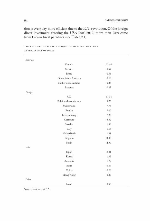
carlos obregón94
tion is everyday more efficient due to the ICT revolution. Of the foreign direct investment entering the USA 2003-2012, more than 25% came from known fiscal paradises (see Table 2.1).
table 2.1. usa fdi inwards 2003-2012. selected countries
as percentage of total
Americas
Canada 11.48
Mexico 0.57
Brazil 0.36
Other South America 0.10
Netherlands Antilles 0.28
Panama 0.27
Europe
UK 17.31
Belgium-Luxembourg 9.73
Switzerland 7.76
France 7.40
Luxembourg 7.29
Germany 6.52
Sweden 1.60
Italy 1.16
Netherlands 1.08
Belgium 3.09
Spain 2.99
Asia
Japan 8.81
Korea 1.33
Australia 1.72
India 0.37
China 0.26
Hong Kong 0.33
Other
Israel 0.68
Source: same as table 1.5.

nationalism and changes in the income distribution 95
The real reason that the developed nations’ governments do not come to an agreement to disappear the fiscal paradises is that these countries benefit, in a privilege manner, from the money coming from such para-dises —whose origins are largely in the developing economies. The conse-quences, however, are unwelcome. One of them is that the governments are losing control of their fiscal policy, because fiscal paradises make capi-tal very mobile. However, there are several others. Fiscal paradises are key for money laundering, and therefore, foster corruption, and criminal and terrorist’s activities.
In respect to the within country income distribution, it has not wors-ened in all the countries. There are very different institutional responses to the ICT revolution. The concentration of income was worse in the Anglo-Saxon countries, because they had weaker social policies as com-pared to other European countries.
The main problem of the world today is not the worsening of the with-in country income distribution in the Anglo-Saxon world, but the lack of proper global governance. The old neoliberal economic ideas were unable to: maintain employment and financial stability in the developed world; create economic growth in the middle-income economies that follow the recommended neoliberal policies; and to move out of poverty at many of the countries that were with urgent needs. The world is not facing in a proper manner the rapid changes brought about by the ICT revolution.
As Milanovic recognizes over and over in his recent magnificent 2016 book, we cannot really forecast the future, but the implications go further than he himself recognizes. Not only are there no long-term laws of capital-ism that necessarily concentrate income as Piketty 2014 has suggested, nei-ther is there the possibility to forecast the future using Milanovic’s Kuznets waves. As Karl Popper once said, innovation is about what we do not know. We do not know what the future will bring —we simply cannot forecast it.
The globalization phenomenon has made trade decisive for income distribution. The worsening of the income distribution in the Unit-ed States could not be understood without China. Since trade and growth are closely related, it means that we cannot look at the income distribution phenomena without discussing technological change and economic growth.
If we state the income distribution question only in distribution terms, for example: whether the middle class in America is worse off versus the rich? And we propose to analyze: which are the policy options? The an-swer would most likely involve nationalism and protectionism, as it did
carlos obregón96
in the USA’s presidential campaigns of both Mr. Trump and Mr. Sand-ers —despite their contradictory ideologies. The answer will involve the incorrect economic logic, which goes as follows: If companies do not go to China or Mexico, there will be more jobs for USA citizens.
The question in instead has to be posed taking into account techno-logical and economic growth considerations. Is America as a country bet-ter or worse off because American companies going to China or Mexico? Is the middle class in general in America better or worse off in absolute terms? Can the ICT revolution really be stopped, and which will be the consequences for the American economy both short and long-term? Asking the right question will take us to very different policy recommen-dations. And of course, as a separate issue, one should ask: whether the world is better or worse off because of China?
Today, analyzing the whole world is imperative because technology has connected it. The critical point to understand is that the ICT revo-lution has brought us closer to one another, and like any technological revolution, it cannot be stopped. It will happen anyway in the long run. But if institutions do not accommodate it, the process will be painful and costly in economic terms. Particularly for the countries that resist it, in this case the USA and the UK, but also for the global economy.
The history of the last two centuries was decided by three global phe-nomena —none of them linked to the class conflict envisioned by Marx. The first one is the political triumph of the middle class in the developed economies, which translates in a significant appropriation of income by the middle class. From the beginning of the twentieth century to today, the middle class–defined as the lowest 90 percent —took away from the rich— defined as the top ten percent —between 22 and 60% of their dis-posable income in real terms (Table 2.14). This percentage first went up and then down since the 1980s, but taking the whole century, the middle class is a big winner. This is important, because as Adam Smith taught us, development has to do with the size of the markets, which allow for spe-cialization of labor and technological progress. The growth of the middle class in the developed world has been crucial to widen the markets, and this has been decisive not only for the economic development of the West but also for the one of the Asian countries that converge–whose model is based on exporting to the middle class in the developed world.
The second global phenomena is the increasing number of formal democracies in developing countries which lack a true middle class. A middle class, as previously said, is defined by two key elements: 1) Its
nationalism and changes in the income distribution 97
economic capacity of consumption of global goods —produced at the world’s technological frontier—, and 2) Its interest and capability to con-front the high classes as to how the country must be governed. The first element is required not only to enlarge the global market, but to foster a local national market that increasingly adheres itself to global standards. The lack of this first element is behind the failure of communist countries to achieve sustainable economic growth. The second element is required because it is the one that allows the middle class to fight efficiently for in-creasing the size of its piece of the pie in the income distribution. The lack of a truly middle class in many developing economies meant that income has remained, to a much larger extent than in the developed countries, in the hands of the rich.
The lowest 90% has not increased substantially its participation in total income in many countries belonging to the developing world. This is particularly the case with African and Latin American countries. There is however a second group of developing economies, many of them in Asia, which may or may not have formal democracies, but which have traditional political systems that provide adequate governance. In this second group, the income distribution is quite acceptable, being as low in some of them as it is in the Western countries.
The third global phenomena is that the world as a whole today is more unequal than the more inegalitarian countries. The globalization of capitalism did not mean the globalization of the world’s governance. A highly unequal income distribution is, to a large extent, the logical con-sequence of the lack of adequate global governance. In the first group of developing countries mentioned above, the lack of a true middle class al-lows for a much worse income distribution than in the developed world, but anyway, having a common governance, and in many of them an incipient democracy, meant that the masses do have some relative power versus the rich —which at the global level is fully absent.
The problem of income distribution has to be analyzed, as we will, in the broader context of the ICT revolution, globalization, economic growth, and political and social institutions. As North has taught us, so-cieties can change either through technological change or due to social engineering57. The income distribution is a consequence of both.
The ICT revolution has had enormous consequences both in the global income distribution and in the income distribution within coun-tries. We will review in the first section of this chapter the global income
57 North 2005.
carlos obregón98
distribution before and after the ICT revolution. The impact of the ICT revolution has been of such magnitude that for the first time, due to it, the global income distribution has improved, mainly because of the large numbers of the Chinese whom had increased their income —although re-cently India and other Asian countries have also had a noticeable impact. Overall, the world income distribution is still extremely unjust showing the lack of adequate global governance.
In the second section of this chapter we will take a closer look at the within country income distribution. We will show that, due to the ICT revolution there is an increasing tendency towards income distribution deterioration, particularly in developed countries. Which however varies substantially from country to country —due to the specific institutional arrangements, social engineering, and policy responses in each country.
the global income distribution
There is not one, but several global distributions of income that should interest us. The first one, is the between countries income distribution non-weighted by their population. This is a measure of the imputed citi-zenship relative rent that each individual accrues just by being a citizen of one country versus another. As we will see, relative rents are highly unequal and its inequality has not gotten down. They reflect the fact that globalization has not happened at the expense of nationalism. The world was and is defined by national interest and not by class conflict. The sec-ond is the global income distribution between countries weighted by their population. This takes into account the relative population relevance of each country. It can be conceptualized as the proportion of the total glob-al income distribution inequality between individuals that comes from the between countries inequality. As we will explain, inequality in this measure has been recently going down mainly due to China. The third one is the truly global income distribution amongst individuals which conceptually can be seen as the sum of two components58: 1) The pro-portion of the total global income distribution inequality between indi-viduals, that comes from the between countries inequality (measure two);
58 If we measure the inequality with the Theil coefficient —with the property that it can be added up— the result is strictly the sum. If the inequality is measured by the Gini coefficient, there is a remanent.

nationalism and changes in the income distribution 99
and 2) The proportion of the total global income distribution inequality between individuals, that comes from the within country inequality. This third measure expresses the inequality amongst individuals in the world independently of their country of origin. In what follows, we will discuss each one of them.
The between countries global income distribution: non weighted by their population
The calculation is done obtaining the selected inequality index of the PPP GDP per capita at constant prices from the different nations in-volved. Several inequality indexes can be used, such as the Theil index or the Gini coefficient. The results will vary depending upon the PPP series used, because each one of them uses distinct ways to estimate the price differentials between countries. As previously mentioned, there are three PPP series often used: Maddison’s 1990, World Bank’s 2005, and World Bank’s 2011. One of the main and critical differences is that China’s pric-es are higher in the 2005 and 2011 PPPs, therefore China’s GDP is smaller in both of them than in Maddison’s59. The only one of the three series that was estimated for a very long period was Maddison’s.
Table 2.2 presents the GDP per capita in 1990 PPP’s and the cor-responding between regions global inequality Gini coefficients since year 1 after Christ. These Ginis do not indicate the real inequality between countries —because they do not reflect the inequalities of countries be-longing to the same region. But they have the advantage that they can be calculated for more than two thousand years. There are two lessons to learn from this table. The first one is that everybody has benefited from development. In 2010 the standard of living in Africa is 4.3 times better than in the year 1.
But the second one is that development has been very unequal. While Africa improved 4.3 times in 2009 years, the Western Offshoots, which include the USA, improved 73.9 times, and the 30 countries represent-ing Europe, 36.3 times. Eastern Europe and Ex USSR improved more than the world average; Latin America improved as the World aver-age, and Asia and Africa less. In recent decades 1980-2010, all the re-gions improved less than the world average, except Asia, that improved 59 See Table 2.4

carlos obregón100
substantially more. The two regions that improved the least are former USSR and Latin America —they improved less than Africa. For Europe 30 and the Western Offshoots the standard of living improvement is only slightly less than the world average. The Gini coefficient in the bottom of Table 2.2 shows that historically economic development has always brought about more inequality. The rise of inequality starts with global-ization around 1500, and continues increasing the next 450 years. The exception is the last 60 years, in which inequality has remained fairly stable, although at the highest historical level.
table 2.2. gdp per capita, 1990 dollars
Year: 1 1000 1500 1820 1870 1913 1950 1980 2008 2010
Europe 30 576 427 771 1455 2006 3488 4517 13118 21518 20889
Western offshoots
400 400 400 1302 2419 5233 9268 18060 30211 29564
Easter Europe
412 400 496 683 953 1726 2088 5829 8696 8678
Former USSR
400 400 499 680* 943* 1414 2841 6427 7878 7733
Latin America 36
400 400 416 628 776 1552 2505 5437 7028 6767
Asia 45 456 470 568 591 548 691 716 2030 5596 6307
Africa 472 425 414 486 648 908 889 1515 1925 2034
World 467 453 566 712 884 1543 2104 4511 7626 7814
Gini 6.68 2.83 12.06 21.05 29.31 36.35 42.14 39.68 40.82 39.62
Sources: for years 1, 1000, 1500 and for USSR 1820 and 1870 are from Angus Maddison 2009; the rest from Maddison Project 2013, except Gini which is our own calculation.
The global economy is nations’ world. The global economy is not con-stituted by regions but by nations. The nation where one is born gives us a significant imputed citizenship relative rent. This is confirmed by obtaining the Gini inequality between countries —from Maddison 2009 series— for 1913, 1980, and 2008; it gives us .328 for 1913, .523 for 1980, and .523 for 2008. The inequality of the citizenship rents went up substantially between 1913 and 1980, and has remained there. Therefore, one can conclude that —given the migration barriers— the world is a very unfair place, where just
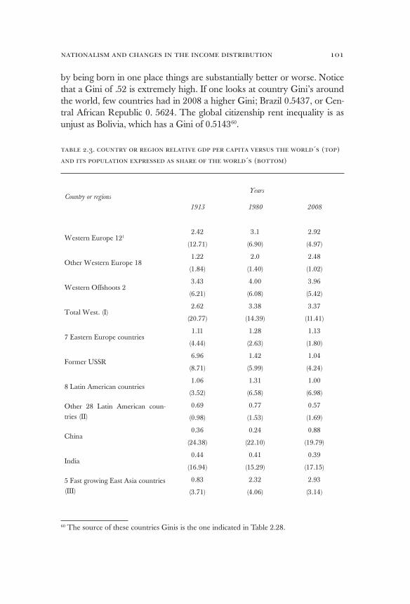
nationalism and changes in the income distribution 101
by being born in one place things are substantially better or worse. Notice that a Gini of .52 is extremely high. If one looks at country Gini’s around the world, few countries had in 2008 a higher Gini; Brazil 0.5437, or Cen-tral African Republic 0. 5624. The global citizenship rent inequality is as unjust as Bolivia, which has a Gini of 0.514360.
table 2.3. country or region relative gdp per capita versus the world´s (top)
and its population expressed as share of the world´s (bottom)
Country or regionsYears
1913 1980 2008
Western Europe 1212.42 3.1 2.92
(12.71) (6.90) (4.97)
Other Western Europe 181.22 2.0 2.48
(1.84) (1.40) (1.02)
Western Offshoots 23.43 4.00 3.96
(6.21) (6.08) (5.42)
Total West. (I)2.62 3.38 3.37
(20.77) (14.39) (11.41)
7 Eastern Europe countries1.11 1.28 1.13
(4.44) (2.63) (1.80)
Former USSR6.96 1.42 1.04
(8.71) (5.99) (4.24)
8 Latin American countries1.06 1.31 1.00
(3.52) (6.58) (6.98)
Other 28 Latin American coun-tries (II)
0.69 0.77 0.57
(0.98) (1.53) (1.69)
China0.36 0.24 0.88
(24.38) (22.10) (19.79)
India0.44 0.41 0.39
(16.94) (15.29) (17.15)
5 Fast growing East Asia countries (III)
0.83 2.32 2.93
(3.71) (4.06) (3.14)
60 The source of these countries Ginis is the one indicated in Table 2.28.
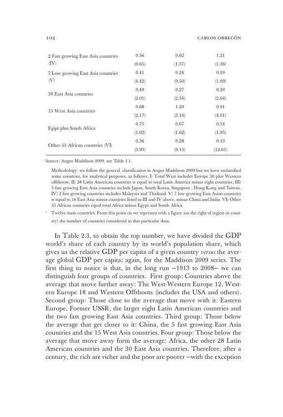
carlos obregón102
2 Fast growing East Asia countries (IV)
0.56 0.62 1.21
(0.65) (1.37) (1.36)
7 Low growing East Asia countries (V)
0.41 0.24 0.59
(4.42) (9.50) (1.09)
30 East Asia countries0.49 0.27 0.30
(2.01) (2.34) (2.64)
15 West Asia countries0.68 1.20 0.91
(2.17) (3.16) (4.01)
Egipt plus South Africa0.75 0.67 0.54
(1.02) (1.62) (1.95)
Other 55 African countries (VI)0.36 0.28 0.19
(5.93) (9.15) (12.61)
Source: Angus Maddison 2009, see Table 1.1.
Methodology: we follow the general classification in Angus Maddison 2009 but we have reclassified some countries, for analytical purposes, as follows: I) Total West includes Europe 30 plus Western offshoots; II) 28 Latin American countries is equal to total Latin America minus eight countries; III) 5 fast growing East Asia countries include Japan, South Korea, Singapore , Hong Kong and Taiwan. IV) 2 fast growing countries includes Malaysia and Thailand. V) 7 low growing East Asian countries is equal to 16 East Asia minus countries listed in III and IV above, minus China and India. VI) Other 55 African countries equal total Africa minus Egypt and South Africa.
1 Twelve main countries. From this point on we represent with a figure (on the right of region or coun-
try) the number of countries considered in that particular data.
In Table 2.3, to obtain the top number, we have divided the GDP world’s share of each country by its world’s population share, which gives us the relative GDP per capita of a given country versus the aver-age global GDP per capita; again, for the Maddison 2009 series. The first thing to notice is that, in the long run —1913 to 2008— we can distinguish four groups of countries. First group: Countries above the average that move further away: The West-Western Europe 12, West-ern Europe 18 and Western Offshoots (includes the USA and others). Second group: Those close to the average that move with it: Eastern Europe, Former USSR, the larger eight Latin American countries and the two fast growing East Asia countries. Third group: Those below the average that get closer to it: China, the 5 fast growing East Asia countries and the 15 West Asia countries. Four group: Those below the average that move away form the average: Africa, the other 28 Latin American countries and the 30 East Asia countries. Therefore, after a century, the rich are richer and the poor are poorer —with the exception
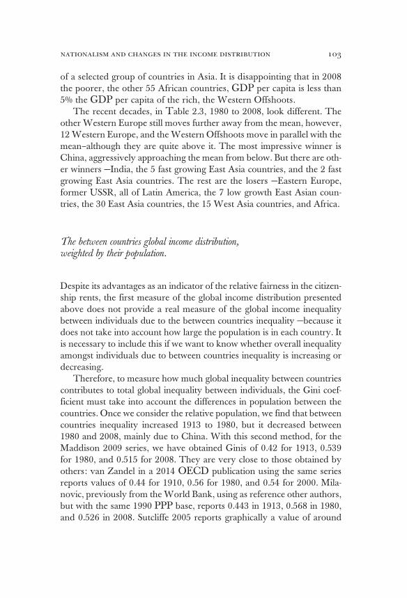
nationalism and changes in the income distribution 103
of a selected group of countries in Asia. It is disappointing that in 2008 the poorer, the other 55 African countries, GDP per capita is less than 5% the GDP per capita of the rich, the Western Offshoots.
The recent decades, in Table 2.3, 1980 to 2008, look different. The other Western Europe still moves further away from the mean, however, 12 Western Europe, and the Western Offshoots move in parallel with the mean–although they are quite above it. The most impressive winner is China, aggressively approaching the mean from below. But there are oth-er winners —India, the 5 fast growing East Asia countries, and the 2 fast growing East Asia countries. The rest are the losers —Eastern Europe, former USSR, all of Latin America, the 7 low growth East Asian coun-tries, the 30 East Asia countries, the 15 West Asia countries, and Africa.
The between countries global income distribution, weighted by their population.
Despite its advantages as an indicator of the relative fairness in the citizen-ship rents, the first measure of the global income distribution presented above does not provide a real measure of the global income inequality between individuals due to the between countries inequality —because it does not take into account how large the population is in each country. It is necessary to include this if we want to know whether overall inequality amongst individuals due to between countries inequality is increasing or decreasing.
Therefore, to measure how much global inequality between countries contributes to total global inequality between individuals, the Gini coef-ficient must take into account the differences in population between the countries. Once we consider the relative population, we find that between countries inequality increased 1913 to 1980, but it decreased between 1980 and 2008, mainly due to China. With this second method, for the Maddison 2009 series, we have obtained Ginis of 0.42 for 1913, 0.539 for 1980, and 0.515 for 2008. They are very close to those obtained by others: van Zandel in a 2014 OECD publication using the same series reports values of 0.44 for 1910, 0.56 for 1980, and 0.54 for 2000. Mila-novic, previously from the World Bank, using as reference other authors, but with the same 1990 PPP base, reports 0.443 in 1913, 0.568 in 1980, and 0.526 in 2008. Sutcliffe 2005 reports graphically a value of around
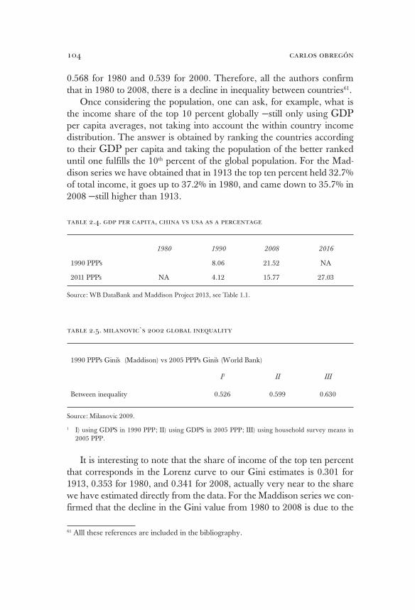
carlos obregón104
0.568 for 1980 and 0.539 for 2000. Therefore, all the authors confirm that in 1980 to 2008, there is a decline in inequality between countries61.
Once considering the population, one can ask, for example, what is the income share of the top 10 percent globally —still only using GDP per capita averages, not taking into account the within country income distribution. The answer is obtained by ranking the countries according to their GDP per capita and taking the population of the better ranked until one fulfills the 10th percent of the global population. For the Mad-dison series we have obtained that in 1913 the top ten percent held 32.7% of total income, it goes up to 37.2% in 1980, and came down to 35.7% in 2008 —still higher than 1913.
table 2.4. gdp per capita, china vs usa as a percentage
1980 1990 2008 2016
1990 PPP´s 8.06 21.52 NA
2011 PPP´s NA 4.12 15.77 27.03
Source: WB DataBank and Maddison Project 2013, see Table 1.1.
table 2.5. milanovic`s 2002 global inequality
1990 PPP`s Gini´s (Maddison) vs 2005 PPP`s Gini´s (World Bank)
I1 II III
Between inequality 0.526 0.599 0.630
Source: Milanovic 2009.
1 I) using GDP`S in 1990 PPP; II) using GDP`S in 2005 PPP; III) using household survey means in 2005 PPP.
It is interesting to note that the share of income of the top ten percent that corresponds in the Lorenz curve to our Gini estimates is 0.301 for 1913, 0.353 for 1980, and 0.341 for 2008, actually very near to the share we have estimated directly from the data. For the Maddison series we con-firmed that the decline in the Gini value from 1980 to 2008 is due to the
61 Alll these references are included in the bibliography.
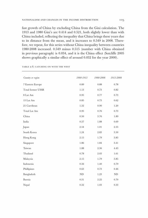
nationalism and changes in the income distribution 105
fast growth of China by excluding China from the Gini calculation. The 1913 and 1980 Gini’s are 0.414 and 0.521, both slightly lower than with China included, reflecting the inequality that China brings these years due to its distance from the mean, and it increases to 0.549 in 2008. There-fore, we repeat, for this series without China inequality between countries 1980-2008 increased. 0.549 minus 0.515 (number with China obtained in previous paragraph) is 0.034, and it is the China effect (Sutcliffe 2005 shows graphically a similar effect of around 0.032 for the year 2000).
table 2.6. catching on with the west
Country or region 1980-1913 1980-2008 1913-2008
7 Eastern Europe 0.89 0.88 0.78
Total former USSR 1.13 0.73 0.82
8 Lat Am 0.95 0.77 0.73
15 Lat Am 0.85 0.73 0.62
21 Carribean 1.32 0.90 1.20
Total Lat Am 0.95 0.76 0.73
China 0.50 3.76 1.89
India 0.37 1.88 0.69
Japan 2.54 1.01 2.55
South Korea 1.24 2.83 3.50
Hong Kong 2.15 1.79 3.85
Singapore 1.86 1.84 3.41
Taiwan 1.88 2.36 4.43
Thailand 0.78 2.03 1.61
Malaysia 2.15 1.79 3.85
Indonesia 0.56 1.40 0.79
Phillipines 0.63 0.73 0.46
Bangladesh ND 1.23 ND
Burnia 0.31 2.22 0.70
Nepal 0.32 1.03 0.33
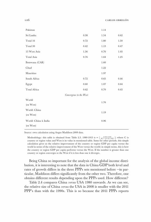
carlos obregón106
Pakistan 1.14
Sri Lanka 0.38 1.54 0.62
Total 16 0.72 1.80 1.30
Total 30 0.42 1.13 0.47
15 West Asia 1.36 0.76 1.03
Total Asia 0.76 1.64 1.25
Botswana (CAR) 1.60
Chad 1.22
Mauritius 1.97
South Africa 0.72 0.65 0.46
Egypt 0.60 1.07 0.64
Total Africa 0.62 0.70 0.43
Convergence to the West:
World
(ex West)1.76
World -China
(ex West)1.19
World -China & India
(ex West)
0.96
Source: own calculation using Angus Maddison 2009 data.
Methodology: this table is obtained from Table 2.3. 1980-1913 is = [ ]; where C is country or region value and West is its value in mentioned table. Same for other periods, this simple calculation gives us the relative improvement of the country or region GDP per capita versus the world in terms of the relative improvement of the West versus the world; in simple terms, this is how the country or region GDP per capita performs versus the West. If the number is greater than one country or region converges to the West if it is less than one it diverges.
Being China so important for the analysis of the global income distri-bution, it is interesting to note that the data in China GDP both level and rates of growth differs in the three PPPs sets mentioned before —in par-ticular, Maddison differs significantly from the other two. Therefore, one obtains different results depending upon the PPPs used. How different?
Table 2.4 compares China versus USA 1980 onwards. As we can see, the relative size of China versus the USA in 2008 is smaller with the 2011 PPP’s than with the 1990s. This is so because the 2011 PPPs reports
nationalism and changes in the income distribution 107
higher prices in China–due to a growing urban China–and therefore less real GDP. Milanovic —formerly from the World Bank— has been argu-ing that the 1990 PPPs used in the Maddison series are wrong, and that they have to be actualized, but nobody has done it. Moreover, it remains as the only series with a long historical perspective. The problem in ad-dition is that data from China is not very good. The 2005 PPPs also had recorded higher prices in China. Milanovic 2009 calculates the between countries global income distribution for year 2002 and obtains 0.53 with the Maddison series, and 0.60 with the 2005 PPP series (see Table 2.5). This is so because China is smaller in relationship to the west in the 2005 PPPs. Thus, the results may vary significantly. Therefore, when comparing results, it is important to remember that PPPs based in 2005 and in 2011 do give a higher global inequality than the Maddison series.
Despite the differences in China’s data, all of the results point out the same direction. The between countries inequality, when measured by an indicator like the Gini coefficient, was higher in 1980 versus 1913, and it is smaller today than in 1980. However, there are differences of opinion as to whether the China effect explains all of between countries inequality re-duction. Using the Maddison 2009 series it does. But using the 2005 PPPs Liberati 2013 found that it does not, it explains only half of the reduction, and that there are other countries involved which explain the other half62.
Let us take a look again at Table 2.3. this time taking in consideration the relative population sizes, bottom indicator Table 2.3. We can divide each region/country top indicator in each year in Table 2.3 by the cor-responding indicator of the total West63. If we get a number greater than one, the region/country is better off than the total West, it converges, and if it is less than one is worse off, it diverges. The results are shown in Table 2.6. Then, we can sum the share of the populations of the cor-responding regions/countries to come up with an estimation of what is the percentage of the global population that is better or worse off than the total West for a given period. We have always taken as a reference the population shares of the last year.
The results are as follows: 1913 to 1980, 86.54% of the population (ex-cluding the West) are worse off; and 1913 to 2008, 73.10% of the popula-tion is worse off. It is only in the period 1980-2008 than less than half of the population is worse off, 46.42%. This seriously questions the convergence
62 Liberati 2013 uses the Penn Tables versión 7. The Penn tables also provide 2005 and 2011 international PPPs at constant prices.
63 Total West = Europe 30 + Western Offshoots as defined by Maddison 2009.
carlos obregón108
between countries weighted by their population sizes. Because even in the best period —1980 to 2008— still almost half of the population —excluding the West— was worse off in 2008 than in 1980 in relationship to total West.
If we restrict ourselves to the period 1980 to 2008, it is relevant to point out that of the 53.58% of the population that is better off in relation-ship to the west 22.3% lives in China, 19.36 in India, and 5.1% in other 7 fast growing Asian countries (5 plus two in Table 2.3). That is 46.76% of the 53.58% of the population that is better off in relationship to the west –1980 to 2008– lives in countries with the Asian Development Model. A model that cannot be extended to the whole world for the simple reason that it is based in exporting substantially more than what is imported.
In the bottom of Table 2.6 we have calculated the world’s convergence to the West for 1980 to 2008, and the number is high 1.76. However, if we take out China it goes down substantially to only 1.19. If we also take out India, the rest of the world diverges from the West —the number goes down to 0.96. This shows how concentrated is the convergence phenomena.
What has happened most recently? Table 2.7 presents similar results to Table 2.6, but this time for the period 1990 to 2016, and based on 2011 World Bank PPPs. It shows relative growth versus total West (as defined in the table). We can see that again China, India, and the fast Asian countries grew faster than the West; but the rest or the World (excluding Japan) grew less than the West, 0.96 the West’s growth. If we add Japan the rest of the world diverges even more, 0.90 the West growth. Even if we add the fast Asian countries, which is equal to the World minus China, minus India, the rest of the World still diverges, 0.95. It is only after adding India that the rest of the World converges to the West —the line represented by world minus China, 1.04.
In summary, convergence is very limited, if we take out China and India the world diverges from the West even as recently as 1990-2016. And this divergence takes place despite the West’s 2008 financial crisis. The West, as defined in the table, grew at annual rate of 1.5% from 1990 to 2016.
The global income distribution between individuals
The previous method assumes that all the individuals in a given country enjoyed the average per capita income, which is not true. Therefore, if we want to obtain the global income distribution between individuals, we have

nationalism and changes in the income distribution 109
to add the within country inequalities. The global income distribution be-tween individuals must include both between countries and within country inequalities.
Within country inequalities can be obtained using diverse sources, such as surveys data, tax data or other supplementary data, which could be based either on deciles of the population or, in the extreme optimal case, in indi-vidual’s data. Tax data is always expressed as market value income, that is before taxes and government’s transfers. Tax underreporting may vary substantially among countries. And at the global level, there is not enough countries’ tax data to construct the global income distribution, but some au-thors use it as reference. Survey’s data usually relates to disposable income, but in the case of some authors, market value income estimates are used. Survey’s data is only available since the mid-eighties, it does not exist for all the years and all the countries, it is inaccurate and to some degree incompat-ible between countries —if for example, the rich respond more surveys in one country than another. Supplementary data may include consumption, disposable monetary incomes and some not specified definitions of income64.
Between countries inequalities can be obtained using as a mean of the distribution GDP per capita or the average household income, consump-tion or expenditures obtained in the surveys. Macroeconomic data like GDP, GDP per capita, population, and in general the macro accounts, is the longest and more accurate set of data.
There are two main methods to obtain the global income distribution between individuals. The first one uses household income distribution sur-veys rescaled by GDP —as a mean, the second one uses both household income distribution surveys and its mean (in instead of the mean GDP)65.
64 Liberati 2013, analyzing the United Nations data base (see Table 2.28 for source reference), for example, reports that: 757 observations refer to disposable income, 319 to consumption, 265 to gross incomes, 242 to disposable monetary incomes and 126 to some not specified definitions of income (disregarding other cases with a smaller number of observations).
65 There are many technical differences between the two methods. The first method, by using decile distribution underestimates inequality because do not take into account the inequality within each decile. The inequality is particularly high in the top decile. The second method, used by Milanovic and others, adds up directly the individuals’ inequality in each country to arrive at a global figure, it uses only surveys data both for the distribution and for the mean. The first method assumes that all the GDP is distributed between the deciles according to the distribution obtained from the surveys data. Missing data is estimated by log normal distribu-tions using the country’s GDP per capita as the mean or by using one year’s known data to substitute missing years. Some studies take Ginis from different countries that correspond to different definitions of income. The goal in all the cases is to add to the between countries in-equality the within country inequality to arrive to a total global inequality number. If theil co-efficients are used they can be added directly; if Gini coefficients are used, overlapping results
carlos obregón110
The results 1988 onwards —with the ICT revolution— are presented in Table 2.8. Three results are obtained with this table:
1. The global income distribution inequality is extremely high, higher than any individual country; in the period 2010 to 2013 is reported in a Gini range of 0.623 to 0.69.
2. The global income distribution is becoming recently less un-equal; between 2008 and 2010 it’s reported as going down in Gini terms between .015 and .009, between 2008 and 2011 .035, and between 2008 and 2013 .043. However, between 1990 and 2010 it is reported as going down between .051 and .08; and between 1988 and 2013 as going down .097. Therefore, for the period 1990 to 2010 or 2013 it went down significantly.
appear from the fact that some income deciles may be richer in poor countries than certain income deciles in rich countries. The advantage of this method is that —thanks to its statistical devices— it can be used for long historical periods. The disadvantage is that when comparing across studies, it becomes impossible to fully understand the consequences of the data het-erogeneity used and/or created through distinct statistical devices. For example, the OECD has shown for many countries and several years that market value income Ginis are much higher than disposable income Ginis. Therefore, we know that estimates by the first method that use market value income data points overestimate within country inequality. If the first method is restricted to the distributional data of disposable income survey data it becomes more accurate, but since such data only exists in reasonable amounts since the mid-eighties, it loses its advantage for providing information for longer periods. Another disadvantage is that distributing GDP by the disposable income decile distribution survey distributes government expenditures minus social expenditures (denoted in what follows as G-S) according to the disposable income shares —an unreasonable assumption. Moreover, the GDP includes some monetary flows that do not accrue to the individual households, such as undistributed firm’s profits. These problems disappear with the second method because instead of using the GDP per capita as the mean, it uses the actual mean income from the surveys. Therefore, G-S is no longer included. The second method —introduced by Milanovic— creates a true global income distribution because it starts with the individual’s disposable income in each country–that is using both the country’s distribution data and its mean. And, as we mentioned before, it has the advantage of eliminating the distorsion introduced by distributing G-S according to the disposable income distribution. But it does not solve the problem of how is G-S distrib-uted? There is a need in the future to study carefully the real distribution of G-S in diverse countries. Today this problem has not been solved. Now it is highly likely that G-S at least in democratic countries is more equally distributed. As an illustration, let us assume that it is distributed in the same proportion to each person; this will imply that the level of inequality is further reduced. This measure is not any longer just disposable income inequality —it could be more properly called income enjoyment inequality. The main problem with using the second method is that the average household income, consumption or expenditures mean obtained in the surveys is much smaller than the income, consumption or expenditures obtained from the macroaccounts —which are more reliable— and particularly in poor countries the difference is bigger. Therefore, the between countries inequality is overestimated —because the poor coun-tries appear as having less income in relation to the more wealthy than what they really have.

nationalism and changes in the income distribution 111
3. It is higher if we use household surveys and its means versus household survey rescaled by GDP. Bourguignon 2015, using the same data set, obtained for 2010 in the first case 0.69, and in the second 0.623 —see footnote 65.
table 2.7. gdp per capita growth versus west’s1
Population % world
2 2016-1990 2016-2008 2008-1990 1990 2008 2016
World 1.15 1.11 1.03 1.00 1.00 1.00
West 1.00 1.00 1.00 14.68 12.78 12.09
China 6.41 1.73 3.71 21.48 19.58 18.53
Japan 0.85 1.01 0.85 2.34 1.89 1.70
India 2.36 1.54 1.54 16.46 17.70 17.79
Fast Asian countries 1.79 1.17 1.52 2.39 2.28 2.21
Rest of the world 0.96 1.05 0.92 42.65 45.75 47.68
Rest of the world plus Japan
0.90 1.03 0.87 44.99 47.64 49.38
World minus China 1.04 1.10 0.95 63.84 67.63 69.38
World minus China & India
0.95 1.04 0.91 47.38 49.93 51.59
Source: WDI DataBank, last update 08/02/2017, see Table 1.1.
1 Methodology: from our own calculations; same methodology as table 2.6. Regional GDP per capitas are estimated using GDP per capita PPP constant 2011 international dollars and total population.
2 West: European Union (28), USA, Canada, Australia and New Zealand. Fast Asian countries: Hong Kong, Singapore, Korea, Thailand and Malaysia.
The ICT revolution meant a rapid rise of the income in China which both: a) Reduced the between countries inequality and b) increased the within country inequality in China and in the developed economies. The overall effect is a decrease in the total global income distribution inequali-ty. However, it remains at a very high level, much higher than any region or country; the highest Gini in 2008 reported for a country or a region in Table 2.9 is .583 for Sub-Saharan Africa versus .705 for the World; the

carlos obregón112
World is by far a more unequal place than Sub-Saharan Africa, hard to understand and accept given the supposed global humanistic values.
table 2.8. global income distrubution (gini)
Household surveys and household surveys means
1990 1995 2000 2005 2008 2010 2013
Bourguignon
(2015)0.741 0.738 0.734 0.712 0.699 0.690
1988 1993 1998 2003 2008 2011
Lakner-Milanovic
(2013)0.722 0.719 0.715 0.719 0.705 0.670
Milanovic
(2016)0.668 0.625
Household surveys data, rescaled by GDP
1990 1995 2000 2005 2008 2010
Bourguignon
(2015)0.703 0.690 0.683 0.658 0.638 0.623
Source as indicated in table.
GDP statistics are more solid than the survey’s data. One of the lat-est problems is that surveys report only a portion of the income that is reflected in national accounts, and in actuality, the proportion is going down. Bourguignon 2015, for the large sample that he uses, reports sur-veys income at 55.8% of GDP in 1990 and at 47.9% in 201066. The fact that global inequality is higher using household surveys versus household surveys rescaled by GDP seems to indicate that poor countries income is underrepresented in the household surveys, likely because they have a higher degree of underreporting from the high class67.
66 P 44.
67 See Bourguignon 2015, p. 43 to 45. Milanovic argues that it is due to sample differences, and to the fact that Bourguignon uses deciles. But since Bourguignon uses the same sample to estimate the results both with GDPs and with the surveys means, and the difference is

nationalism and changes in the income distribution 113
table 2.9. global inequality versus regional
GINI 1988 GINI 2008
World 72.2 70.5
Mature economies 38.2 41.9
China 32.0 42.7
India 31.1 33.1
Other Asia 44.5 45.0
Sub-Saharan Africa*1 53.5 58.3
LatAm and Caribb 52.7 52.8
Russia, Central Asia*, South Caribb 48.3 41.9
Source: Lakner-Milanovic 2013.
1 These regions’ (*) Ginis are from 1993 instead of 1988.
Table 2.10 presents the global income distribution historical Gini from 1820 to 2010. It rises 1820 until 1990 when the ICT revolution starts, and then declines for most authors, although for some of them the declin-ing starts in 2000. As we have previously indicted, the declining 1990 to 2010 is significant; for Bourguignon, the 2010 level goes back to a level almost similar to 1913.
Table 2.11 shows the Gini coefficients for within country inequality and between countries inequality. As it can be seen, in 1820, most of the total global inequality came from within country inequality, however with the rapid development of capitalism between countries inequality rises fast, by 1910 it is even higher than within country inequality, and it remains higher until 2000. Despite the fact that due to the ICT revolution between coun-tries inequality went down (mainly because of China and India) and within country inequality went up (mainly because of China, USA, and other de-veloped economies) between 1990 and 2000; in 2000, between countries inequality is at 0.54 Gini versus a 0.45 Gini for within country inequality.
high and still there, it seems clear that Bourguignon’s hypothesis is superior.
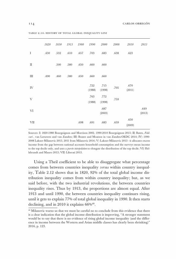
carlos obregón114
table 2.10. history of total global inequality gini
1820 1850 1913 1980 1990 2000 2008 2010 2013
I .430 .532 .610 .657 .703 .683 .638 .623
II .500 .580 .650 .660 .660
III .490 .460 .580 .650 .660 .660
IV.722
(1988).715
(1998).705
.670 (2011)
V.763
(1988)
.772
(1998).759
VI.687
(2003).649
(2013)
VII .698 .691 .683 .659.650
(2009)
Sources: I) 1820-1980 Bourguignon and Morrison 2002, 1990-2010 Bourguignon 2015; II) Baten, Fold-
vari , van Leeuwen and van Zanden; III) Boates and Moatsos in van Zanden-OEDC 2014; IV) 1990-2008 Lakner-Milanovic 2013, 2011 from Milanovic 2016; V) Lakner-Milanovic 2013 –it allocates excess income from the gap between national accounts household consumption and the surveys mean income to the top decile only, and uses a pareto interpolation to elongate the distribution of the top decile; VI) Hel-lebrandt and Mauro 2013; VII) Liberati 2013.
Using a Theil coefficient to be able to disaggregate what percentage comes from between countries inequality versus within country inequal-ity, Table 2.12 shows that in 1820, 92% of the total global income dis-tribution inequality comes from within country inequality; but, as we said before, with the two industrial revolutions, the between countries inequality rises. Thus by 1913, the proportions are almost equal. After 1913 and until 1990, the between countries inequality continues rising, until it gets to explain 77% of total global inequality in 1990. It then starts declining, and in 2010 it explains 66%68.68 Milanovic warns us that we must be careful no to conclude from this evidence that there is a clear indication that the global income distribution is improving, “A stronger statement would be to say that there is no evidence of rising global income inequality (and the differ-ence in income between the Western and Asian middle classes has clearly been shrinking)” 2016, p. 123.
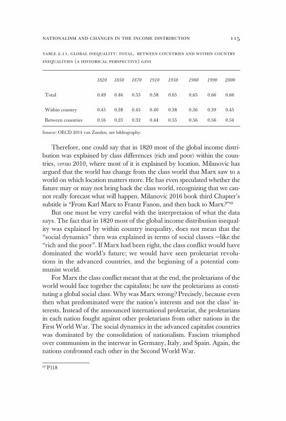
nationalism and changes in the income distribution 115
table 2.11. global inequality: total, between countries and within country
inequalities (a historical perspective) gini
1820 1850 1870 1910 1950 1980 1990 2000
Total 0.49 0.46 0.55 0.58 0.65 0.65 0.66 0.66
Within country 0.45 0.38 0.45 0.40 0.38 0.36 0.39 0.45
Between countries 0.16 0.23 0.32 0.44 0.55 0.56 0.56 0.54
Source: OECD 2014 van Zanden, see bibliography.
Therefore, one could say that in 1820 most of the global income distri-bution was explained by class differences (rich and poor) within the coun-tries, versus 2010, where most of it is explained by location. Milanovic has argued that the world has change from the class world that Marx saw to a world on which location matters more. He has even speculated whether the future may or may not bring back the class world, recognizing that we can-not really forecast what will happen. Milanovic 2016 book third Chapter’s subtitle is “From Karl Marx to Frantz Fanon, and then back to Marx?”69
But one must be very careful with the interpretaion of what the data says. The fact that in 1820 most of the global income distribution inequal-ity was explained by within country inequality, does not mean that the “social dynamics” then was explained in terms of social classes —like the “rich and the poor”. If Marx had been right, the class conflict would have dominated the world’s future; we would have seen proletariat revolu-tions in the advanced countries, and the beginning of a potential com-munist world.
For Marx the class conflict meant that at the end, the proletarians of the world would face together the capitalists; he saw the proletarians as consti-tuting a global social class. Why was Marx wrong? Precisely, because even then what predominated were the nation’s interests and not the class’ in-terests. Instead of the announced international proletariat, the proletarians in each nation fought against other proletarians from other nations in the First World War. The social dynamics in the advanced capitalist countries was dominated by the consolidation of nationalism. Fascism triumphed over communism in the interwar in Germany, Italy, and Spain. Again, the nations confronted each other in the Second World War.
69 P118
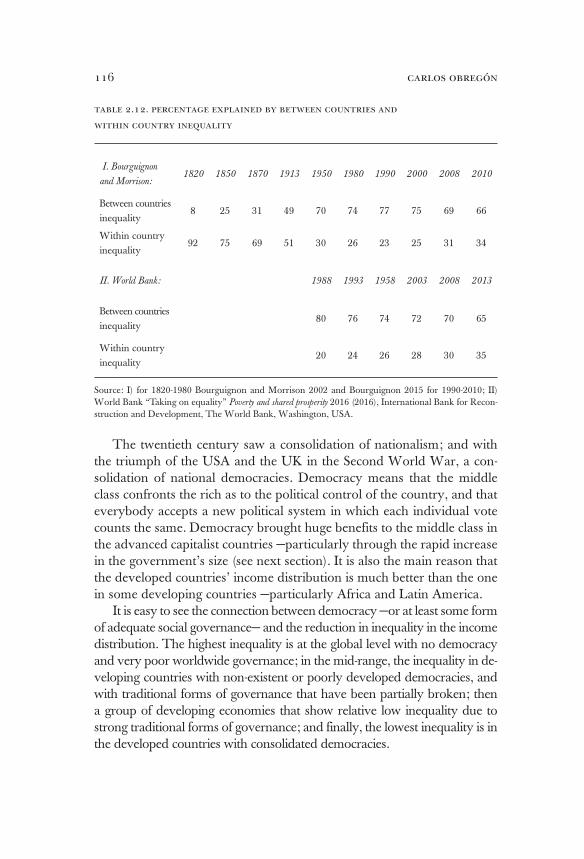
carlos obregón116
table 2.12. percentage explained by between countries and
within country inequality
I. Bourguignon
and Morrison:1820 1850 1870 1913 1950 1980 1990 2000 2008 2010
Between countries inequality
8 25 31 49 70 74 77 75 69 66
Within country inequality
92 75 69 51 30 26 23 25 31 34
II. World Bank: 1988 1993 1958 2003 2008 2013
Between countries inequality
80 76 74 72 70 65
Within country inequality
20 24 26 28 30 35
Source: I) for 1820-1980 Bourguignon and Morrison 2002 and Bourguignon 2015 for 1990-2010; II) World Bank “Taking on equality” Poverty and shared prosperity 2016 (2016), International Bank for Recon-struction and Development, The World Bank, Washington, USA.
The twentieth century saw a consolidation of nationalism; and with the triumph of the USA and the UK in the Second World War, a con-solidation of national democracies. Democracy means that the middle class confronts the rich as to the political control of the country, and that everybody accepts a new political system in which each individual vote counts the same. Democracy brought huge benefits to the middle class in the advanced capitalist countries —particularly through the rapid increase in the government’s size (see next section). It is also the main reason that the developed countries’ income distribution is much better than the one in some developing countries —particularly Africa and Latin America.
It is easy to see the connection between democracy —or at least some form of adequate social governance— and the reduction in inequality in the income distribution. The highest inequality is at the global level with no democracy and very poor worldwide governance; in the mid-range, the inequality in de-veloping countries with non-existent or poorly developed democracies, and with traditional forms of governance that have been partially broken; then a group of developing economies that show relative low inequality due to strong traditional forms of governance; and finally, the lowest inequality is in the developed countries with consolidated democracies.

nationalism and changes in the income distribution 117
That there are rich and poor does not mean that there is a class conflict, not even that they constitute classes, and much less that we can explain the future social dynamics through the income inequal-ity. A class must have characteristics and interests in common. So-cial classes for the classic economists, even for Marx, were the con-sequences of the production process. The income distribution was seen by the classic economists as the consequence of the production process, and not as the result of the interest’s confrontation between income classes that just want more income.
The globalization of the production process meant that nations did confront their national interest in diverse regions of the world, as it happened with Britain, France, Germany, and eventually the USA. The benefits of globalization were unequal for diverse nations and they fought each other for ripping such benefits. The social dynam-ics from 1820 onwards was dominated by national interests, that is why the total global inequality was more and more explained by the between countries inequality.
Now, the fact that the population weighted between countries in-equality is going down and the within country inequality is going up, does not mean that we are reversing into a class society in any sense. The ICT revolution explains both, through the process of produc-tion. The within country increasing inequality is not the outcome of the bad intentions of the rich; it is the consequence of the change in the global process of production due to the ICT revolution. Also, democracies have the capability to implement the adequate policies to counteract the unwanted income distribution consequences of the ICT revolution, as it is shown by the fact that the income distribution did not deteriorate in all of them. The world social dynamics is clearly dominated by national interest, not by class interest. China succeeded as a nation. The fact that the unweighted between countries inequality is not going down, shows us that what really counts, as much today as before, is the nation to which one belongs. At the end of this chapter, we will go back to the topic of the income distribution and economic classes, but for now we return to our main topic in this section, the global income distribution.
Will between countries inequality continue to go down in the future? The ICT revolution will continue expanding, and therefore it is likely that the between countries inequaity will continue to go down. However, the speed at which it will happen is difficult to forecast. China’s growth
carlos obregón118
is due to two factors, the ICT revolution and the Asian Develop-ment Model. The first one will continue, but as we have seen in the previous chapter, it did not produce significant growth in the host country in the Mexican case. The second factor requires that the host country increases savings significantly, and that it exports more than it imports.
Therefore, to forecast the speed at which the between countries inequal-ity will continue to go down, one needs to forecast mainly three variables:
1. Whether China will continue growing very fast, and whether other Asian countries with large populations can and will fol-low its example.
2. Whether the developed countries will be willing to continue ac-commodating increasing exports from developing economies at the expense of maintaining substantial trade deficits.
3. What is the future growth rate of the developed nations? The answer to 1) is yes, but it will be moderated by 2) as the developed
economies refuse to accommodate more and more imports; and 3) heavily depends upon future technology shocks, which are impossible to forecast today. The interested reader may look more on this in Obregon 201470.
the within country income distribution
There have been recent articles and books by very prestigious scholars related to the concentration of income in the last decades in the developed economies. Such concentration, as we have been arguing, is a consequence of the ICT revolution. But, the impact of the new technology in the in-come distribution has not been the same in all the countries. This clearly shows the relevance of the institutional arrangement. Some scholars, how-ever, Piketty being the most renowned one, had argued that there is a long run tendency in capitalism towards the concentration of income; in fact, they argue that there are long-term laws that dictate such concentration
In this section, we will first review the data as to the long run tenden-cies towards the concentration of income in developed economies, then we will look at the data in recent decades both in developed and develop-ing economies, and finally we discuss the theories of income distribution of the classical economists, Kuznets, Piketty, and Milanovic.70 Whose title is Piketty is Wrong and it is available in the Web. See Bibliography.
nationalism and changes in the income distribution 119
The within country income distribution in the last century
At the country level, there are two sets of data for income distribution. The first one is based upon household surveys —this is the official set of data used by governments, the World Bank (WB) and the OECD. For developed economies, the Luxembourg Income Statistics (LIS) data base is one of the usual references for this type of data. This household survey data has been criticized by Piketty and others on the ground that it likely underestimates the share of income of the very wealthy. They have sug-gested instead a second set of data based upon tax reports —which has the additional advantage that it goes back in time for a much longer period. The disadvantage, of course, is tax underreporting and that the quality of tax data can vary substantially in diverse historical periods and between countries. As we said before, there are not enough countries with tax data to build the global income distribution with this type of data. But at the country level, for several countries, both sets of data are available. There is today not enough research to decide on this data controversy, therefore, to explain reality we are left with two sets of reports that are not compatible.
Let us start with Piketty’s claim that in the long run, the income gets concentrated in favor of the richest, top one or ten percent. Using the WID (World Wealth & Income Database) tax data —the one approved by the mentioned author, we have built the graphs that appear as 2.1.a, 2.1.b, and 2.1c, which shows the percentage earned by the top 10 percent for those countries who report market value income share in the WID data base earlier than 1930. We have divided all the countries reported in three groups. Two of them —the USA and the UK— follow Piketty’s suggested U curve, graph 2.1a. Another two —Germany and Norway— show a flat pattern, graph 2.1b. And the last five —France, Sweden, Den-mark, Netherlands, and New Zealand— show a decreasing trend, Graph 2.1.c. Therefore, in the long run, it remains empirically an open question whether Piketty is right or wrong —even for the tax data. The decision has to be made in theoretical terms. But before going into the theory, let us see what else we can learn from the available data.
From the people’s point of view, what counts is their disposable in-come —that is after taxes and social transfers. This is particularly the case given the fact that the size of government’s expenditures in devel-oped economies grew in the 20th century from less than 10% of GDP to

carlos obregón120
more than 40% and social expenditures that were typically less than one percent of GDP in the beginning of the 20th century, are now between 19% and 31% in the main countries (Table 2.13). Therefore, taxes and social transfers have become extremely important to understand inequal-ity. One cannot state the percentage of income that the top 10 percent has only based upon before tax and transfers information, as the WID tax data does —not in a world where governments have gotten so important.
GRAPH 2.1A. TOP 10% NATIONAL INCOME SHARE
Source: www.wid.word
Sh
are
of
tota
l (%
)
GRAPH 2.1B. TOP 10% NATIONAL INCOME SHARE
Source: www.wid.word
Shar
e of
tota
l (%
)
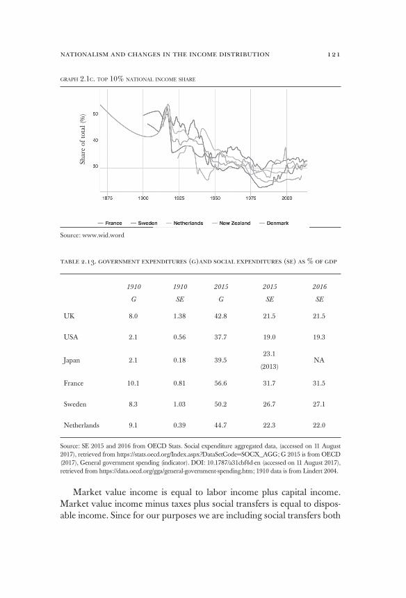
nationalism and changes in the income distribution 121
table 2.13. government expenditures (g)and social expenditures (se) as % of gdp
1910 1910 2015 2015 2016
G SE G SE SE
UK 8.0 1.38 42.8 21.5 21.5
USA 2.1 0.56 37.7 19.0 19.3
Japan 2.1 0.18 39.523.1
(2013)NA
France 10.1 0.81 56.6 31.7 31.5
Sweden 8.3 1.03 50.2 26.7 27.1
Netherlands 9.1 0.39 44.7 22.3 22.0
Source: SE 2015 and 2016 from OECD Stats. Social expenditure aggregated data, (accessed on 11 August 2017), retrieved from https://stats.oecd.org/Index.aspx?DataSetCode=SOCX_AGG; G 2015 is from OECD (2017), General government spending (indicator). DOI: 10.1787/a31cbf4d-en (accessed on 11 August 2017), retrieved from https://data.oecd.org/gga/general-government-spending.htm; 1910 data is from Lindert 2004.
Market value income is equal to labor income plus capital income. Market value income minus taxes plus social transfers is equal to dispos-able income. Since for our purposes we are including social transfers both
GRAPH 2.1C. TOP 10% NATIONAL INCOME SHARE
Source: www.wid.word
Sh
are
of
tota
l (%
)

carlos obregón122
in cash and in kind, we are using social public expenditures as equivalent to social transfers. Therefore, in what follows we will use market value income to imply disposable income plus taxes minus social transfers i.e. social public expenditures. Note that there are two different market val-ues of income, one derived from the tax data and the other from the surveys data. Therefore, one needs to keep always in mind which one of the two is being discuss.
table 2.14. top 10% income share wid data
Market value Disposable income Change %
19101 2013 1910 2013 MV DI
France 51.51 29.81 51.08 20.50 - 42.12 - 59.90
Sweden 43.88 30.62 43.43 21.25 - 30.22 - 51.07
UK 37.03 41.29 36.54 26.83 11.50 - 26.57
US 40.51 45.64 40.25 31.55 12.66 - 21.61
Source: MV share is from World Wealth and Income Data (WID) consulted, August 13 2017. Dispos-able income is calculated with the formula and the notation in text footnote 73. In this formula, SE comes from Public Expenditure in OECD Social expenditure-aggregated data, see Table 2.13; T is total tax revenues from OECD (2017) tax revenue (indicator).doc: 10.1787/d 98b8cfs-en (accessed August 14, 2017). Retrieved from https://data.oecd.org/tax/tax-revenue.htm. OECD presents SE and T as GDP percentages. To obtain Sni and Tni we use GDP and net adjusted national income from the World Bank DataBank available on the web, accessed August 14, 2017. Thus, Sni=[ ] and Tni= [ ]. Sni for1910 is from Lindert (2004) for all countries. Lindert (2004) Growing public social spending and economic growth since the 18th century; vol-the story, Cambridge University Press. Tni for 1910 from Piketty (2014) tables TS 13.1 detailed series. The t and s are as indicated in Table 2.16.
1 France and Sweden 1910, UK 1918, US 1917.
What does all this mean for the long-term comparison between the income distribution at the beginning of the twentieth century versus to-day? In Table 2.14, on the left side we present Piketty’s and the WID data for the MV share of the top 10 percent in four countries with long-term available data, France, Sweden, United Kingdom, and the USA71. It shows what we already mentioned before, that many countries do not show, even in the MV-WID- share, Piketty’s U curve —this is the case for France and Sweden. France top 10% share goes down from 51.5% to 29.8%, and Sweden from 43.9% to 30.6%.71 Since in the middle columns we want to estimate disposable income we need long-term data both for taxes and social expenditures.
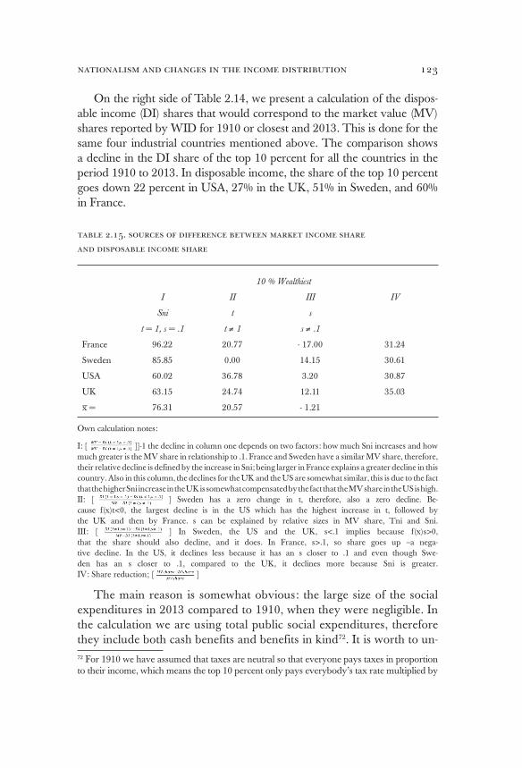
nationalism and changes in the income distribution 123
On the right side of Table 2.14, we present a calculation of the dispos-able income (DI) shares that would correspond to the market value (MV) shares reported by WID for 1910 or closest and 2013. This is done for the same four industrial countries mentioned above. The comparison shows a decline in the DI share of the top 10 percent for all the countries in the period 1910 to 2013. In disposable income, the share of the top 10 percent goes down 22 percent in USA, 27% in the UK, 51% in Sweden, and 60% in France.
table 2.15. sources of difference between market income share
and disposable income share
10 % Wealthiest
I II III IV
Sni t s
t = 1, s = .1 t ≠ 1 s ≠ .1
France 96.22 20.77 - 17.00 31.24
Sweden 85.85 0.00 14.15 30.61
USA 60.02 36.78 3.20 30.87
UK 63.15 24.74 12.11 35.03
x = 76.31 20.57 - 1.21
Own calculation notes:
I: [
]]-1 the decline in column one depends on two factors: how much Sni increases and how much greater is the MV share in relationship to .1. France and Sweden have a similar MV share, therefore, their relative decline is defined by the increase in Sni; being larger in France explains a greater decline in this country. Also in this column, the declines for the UK and the US are somewhat similar, this is due to the fact that the higher Sni increase in the UK is somewhat compensated by the fact that the MV share in the US is high. II: [ ] Sweden has a zero change in t, therefore, also a zero decline. Be-cause f(x)t<0, the largest decline is in the US which has the highest increase in t, followed by the UK and then by France. s can be explained by relative sizes in MV share, Tni and Sni. III: [ ] In Sweden, the US and the UK, s<.1 implies because f(x)s>0, that the share should also decline, and it does. In France, s>.1, so share goes up –a nega-tive decline. In the US, it declines less because it has an s closer to .1 and even though Swe-den has an s closer to .1, compared to the UK, it declines more because Sni is greater. IV: Share reduction; [ ]
The main reason is somewhat obvious: the large size of the social expenditures in 2013 compared to 1910, when they were negligible. In the calculation we are using total public social expenditures, therefore they include both cash benefits and benefits in kind72. It is worth to un-72 For 1910 we have assumed that taxes are neutral so that everyone pays taxes in proportion to their income, which means the top 10 percent only pays everybody’s tax rate multiplied by
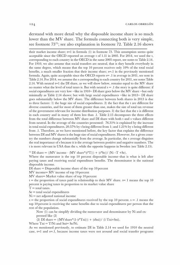
carlos obregón124
derstand with more detail why the disposable income share is so much lower than the MV share. The formula connecting both is very simple, see footnote 7373; see also explanation in footnote 72. Table 2.16 shows
their market income share; t=1 in formula (1) in footnote 73. This assumption seems quite acceptable since the OECD reported an average t of 1.11 in 2005. For 2014, we used the t, corresponding to each country in the OECD in the same 2005 report, see notes to Table 2.14. For 1910, we also assume that social transfers are neutral, that is they benefit everybody in the same degree, which means that the top 10 percent receives only 10% of the total social benefits, a much smaller fraction that their income share; s=.1 in the previously mentioned formula. Again, quite acceptable since the OECD reports s= .1 in average in 2011, see note in Table 2.14. For 2014, we assume the s corresponding to each country for 2011, see notes Table 2.14. With neutral t=1 the DI share, as we will show below, remains equal to the MV share no matter what the level of total taxes is. But with neutral s = .1 the story is quite different: if social expenditures are very low —like in 1910— DI share goes below the MV share —but only minimally as Table 2.14 shows; but with large social expenditures —like in 2013— DI share goes substantially below the MV share. The difference between both shares in 2013 is due to three factors: 1) the huge size of social expenditures. 2) the fact that the t are different for diverse countries, and for most of them greater than one, makes the size of total tax revenue of the government relevant for income distribution purposes. 3) the fact that the s is different in each country and in many of them less than .1. Table 2.15 decomposes the three effects from the total difference between MV share and DI share with both t and s values different from neutral. In the average of the countries presented: 76.31% is explained by the increase in total social expenditures, 20.57% by t being different from 1; and 1.21% by s being different from .1. Therefore, as we have mentioned before, the key factor that explains the difference between DI and MV shares is the huge size of social expenditures. However, for a given coun-try the numbers change substantially from the average. In particular, the s average disguises the real importance of s because it is the average between positive and negative numbers. The t is more relevant in USA than the s, while the opposite happens in Sweden (see Table 2.15).
73 DI share = ((MV income - (MV share*(t*T))) + (s*Se))/ (Ni –T +Se). Where the numerator is the top 10 percent disposable income–that is what is left after paying taxes and receiving social expenditure benefits. The denominator is the national disposable income.DI share = Disposable income share of the top 10 percentMV income= MV income of top 10 percentMV share= Market value share of top 10 percentt = the proportion of taxes paid in relationship to their MV share. t= 1 means the top 10
percent is paying taxes in proportion to its market value shareT = total taxes.Se = total social expendituresNi = net adjusted national income s = the proportion of social expenditures received by the top 10 percent. s = .1 means the top 10 percent is receiving the same benefits due to social expenditures per person that the rest of the population.
Now (1) can be simplify dividing the numerator and denominator by Ni and ex-pressed like (2)(2) DI share = ((MVshare*(1-(t*Tni))) + (sSni))/ (1-Tni+Sni).
Where Tni = T/Ni and Sni= Se/Ni. As we mentioned previously, to estimate DI in Table 2.14 we used for 1910 the neutral case, t=1 and s=.1, because income taxes were not around and social transfer programs
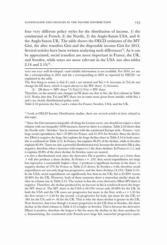
nationalism and changes in the income distribution 125
four very different policy styles for the distribution of income. 1) the continental or French, 2) the Nordic, 3) the Anglo-Saxon USA, and 4) the Anglo-Saxon UK. The table shows the OECD estimates of the MV Gini, the after transfers Gini and the disposable income Gini for 2013. Several articles have been written analyzing such differences74. As it can be appreciated, social transfers are more important in France, the UK, and Sweden, while taxes are more relevant in the USA (see also tables 2.14 and 2.15)75.
were not very well developed —and reliable information is not available. For 2014, we use the s corresponding to 2011 and the t corresponding to 2005 as reported by OECD —as explained in the table.The first thing to notice is that if t and s are neutral and Sni = 0, increases in Tni do not change the DI share, which is equal always to the MV share. (1) becomes
(1) DI share = (MV share *(1-Tni))/(1-Tni) = MV shareTherefore, in the neutral case changes in DI share are due to Sni, the first column in Table 2.15. Notice also that Tni and MV share are in some sense given from outside, while Sni, t and s are clearly distributional policy tools. Table 2.16 presents the Sni, t and s values for France, Sweden, USA, and the UK.
74 Look at OECD Income Distribution studies, there are several articles in here related to this topic.
75 Since the Gini measures inequality all along the Lorenz curve, one should not expect a close relation with our inequality 10/90 measure, however there is a relation. Table 2.16 shows that the Nordic style —Sweden— has in common with the continental Europe style —France— very large social expenditures, Sni = 37.80% for France, and 31.97% for Sweden. Since the deriva-tive DIsni is negative the large, Sni explains the huge decline share in Table 2.14 in both cases; this is confirmed in Table 2.15. In France, Sni explains 96.2% of the decline, while in Sweden explains 85.9%. Taxes are also a powerful distributional tool, because the derivative DIt is also negative, therefore when t increases with respect to 1 the share declines. In France t= 1.1, and it explains 20.8% of the share decline. In Sweden, taxes are neutral. s is also a distributional tool, since the derivative Dis is positive, therefore an s lower than .1 will also produce a share decline. In France s = .135, thus social expenditures are large but regressive; a sustantially higher s than .1 produces a significant increase in the share —a negative decline of 17% for France as Table 2.15 shows. In Sweden s =.66, therefore social expenditures are not only large but progressive, and the share declines 14.15% (Table 2.15). In the USA, social expenditures are significantly less than in the UK; Sni is 21.89% versus 26.80% for the UK. However, both of these countries show a somewhat similar share de-cline in column one in Table 2.15. The reason is that the cross derivative DIsni MVshare is negative. Therefore, the decline produced by an increase in Sni is reinforced more the larger the MV share is. The MV share in the USA is 30.15% versus only 25.68% for the UK. In both the USA and the UK taxes are progressive but more in the first; with a t = 1.35 for the first versus t = 1.20 for the second. s is progressive for both, but more for the UK; s= .081 for the US, and s= .04 for the UK. That is why the share decline is greater in the UK. Note however, that even though s is more progressive in the UK than in Sweden, the share decline in the third column in Table 2.15 is higher in Sweden. This is because the derivative DIssni is positive, therefore the largest is Sni the more the decline in the share produce by s. Summarizing: the continental style–French–uses large Sni, somewhat progressive taxes,
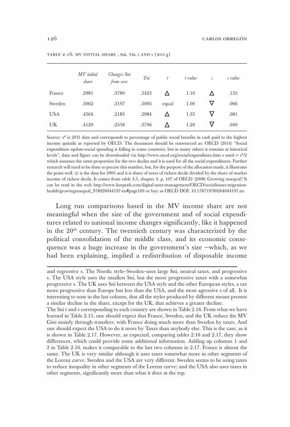
carlos obregón126
table 2.16. mv initial share , sni, tni, t and s (2014)
MV initial
share
Changes Sni
from zeroTni t t value s s value
France .2981 .3780 .5423 1.10 .135
Sweden .3062 .3197 .5005 equal 1.00 .066
USA .4564 .2183 .2984 1.35 .081
UK .4129 .2558 .3796 1.20 .040
Source: s* is 2011 data and corresponds to percentage of public social benefits in cash paid to the highest income quintile as reported by OECD. The document should be outsourced as: OECD (2014) “Social expenditure update-social spending is falling in some countries, but in many others it remains at historical levels”, data and figure can be downloaded via http://www.oecd.org/social/expenditure.htm s used = s*/2 which assumes the same proportion for the two deciles and it is used for all the social expenditures. Further research will need to be done to precise this number, but, for the purpose of the allocation made, it illustrates the point well. (t) is the data for 2005 and it is share of taxes of richest decile divided by the share of market income of richest decile. It comes from table 4.5, chapter 4, p, 107 of OECD (2008) Growing unequal? It can be read in the web http://www.keepeek.com/digital-asset-management/OECD/socialissues-migration-health/growingunequal_978926044197-en#page109 or buy as OECD DOI: 10.178719789264044197.en
Long run comparisons based in the MV income share are not meaningful when the size of the government and of social expendi-tures related to national income changes significantly, like it happened in the 20th century. The twentieth century was characterized by the political consolidation of the middle class, and its economic conse-quence was a huge increase in the government’s size —which, as we had been explaining, implied a redistribution of disposable income
and regressive s. The Nordic style–Sweden–uses large Sni, neutral taxes, and progressive s. The USA style uses the smallest Sni, but the more progressive taxes with a somewhat progressive s. The UK uses Sni between the USA style and the other European styles, a tax more progressive than Europe but less than the USA, and the most agressive s of all. It is interesting to note in the last column, that all the styles produced by different means present a similar decline in the share, except for the UK, that achieves a greater decline. The Sni t and s corresponding to each country are shown in Table 2.16. From what we have learned in Table 2.15, one should expect that France, Sweden, and the UK reduce the MV Gini mainly through transfers; with France doing much more than Sweden by taxes. And one should expect the USA to do it more by Taxes than anybody else. This is the case, as it is shown in Table 2.17. However, as expected, comparing tables 2.16 and 2.17, they show differences, which could provide some additional information. Adding up columns 1 and 3 in Table 2.16, makes it comparable to the last two columns in 2.17. France is almost the same. The UK is very similar although it uses taxes somewhat more in other segments of the Lorenz curve. Sweden and the USA are very different. Sweden seems to be using taxes to reduce inequality in other segments of the Lorenz curve; and the USA also uses taxes in other segments, significantly more than what it does at the top.
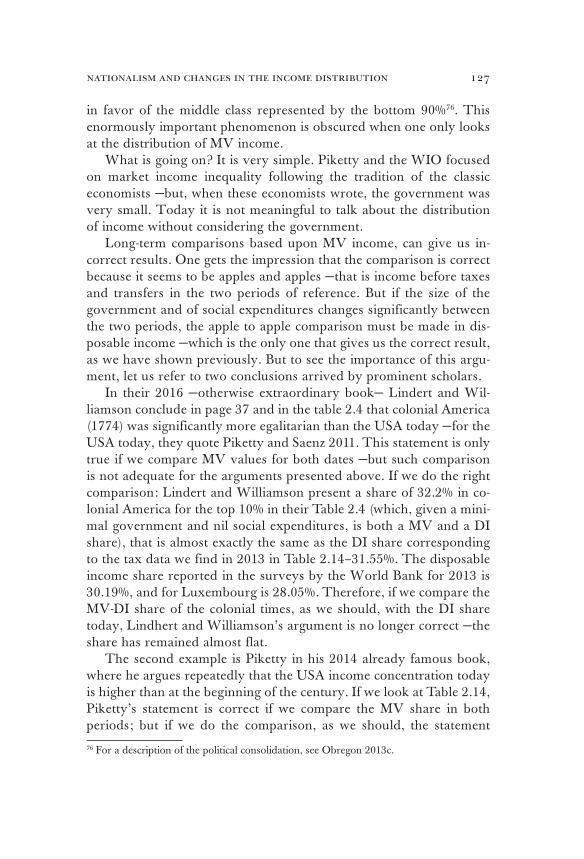
nationalism and changes in the income distribution 127
in favor of the middle class represented by the bottom 90%76. This enormously important phenomenon is obscured when one only looks at the distribution of MV income.
What is going on? It is very simple. Piketty and the WIO focused on market income inequality following the tradition of the classic economists —but, when these economists wrote, the government was very small. Today it is not meaningful to talk about the distribution of income without considering the government.
Long-term comparisons based upon MV income, can give us in-correct results. One gets the impression that the comparison is correct because it seems to be apples and apples —that is income before taxes and transfers in the two periods of reference. But if the size of the government and of social expenditures changes significantly between the two periods, the apple to apple comparison must be made in dis-posable income —which is the only one that gives us the correct result, as we have shown previously. But to see the importance of this argu-ment, let us refer to two conclusions arrived by prominent scholars.
In their 2016 —otherwise extraordinary book— Lindert and Wil-liamson conclude in page 37 and in the table 2.4 that colonial America (1774) was significantly more egalitarian than the USA today —for the USA today, they quote Piketty and Saenz 2011. This statement is only true if we compare MV values for both dates —but such comparison is not adequate for the arguments presented above. If we do the right comparison: Lindert and Williamson present a share of 32.2% in co-lonial America for the top 10% in their Table 2.4 (which, given a mini-mal government and nil social expenditures, is both a MV and a DI share), that is almost exactly the same as the DI share corresponding to the tax data we find in 2013 in Table 2.14–31.55%. The disposable income share reported in the surveys by the World Bank for 2013 is 30.19%, and for Luxembourg is 28.05%. Therefore, if we compare the MV-DI share of the colonial times, as we should, with the DI share today, Lindhert and Williamson’s argument is no longer correct —the share has remained almost flat.
The second example is Piketty in his 2014 already famous book, where he argues repeatedly that the USA income concentration today is higher than at the beginning of the century. If we look at Table 2.14, Piketty’s statement is correct if we compare the MV share in both periods; but if we do the comparison, as we should, the statement
76 For a description of the political consolidation, see Obregon 2013c.
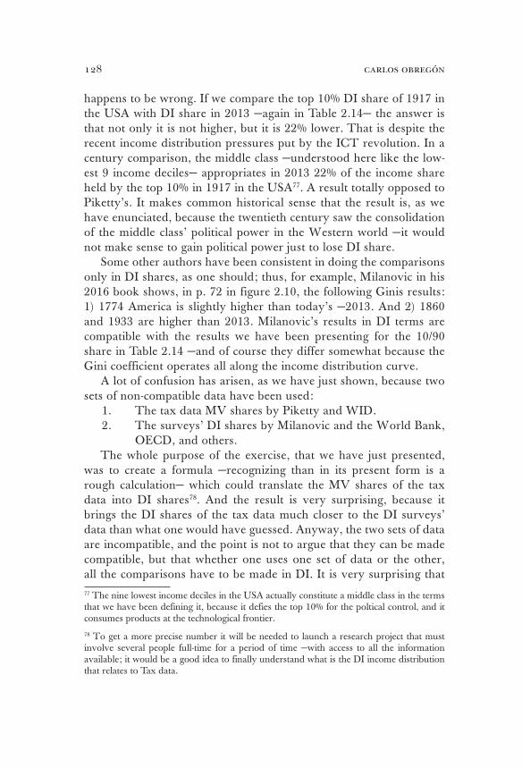
carlos obregón128
happens to be wrong. If we compare the top 10% DI share of 1917 in the USA with DI share in 2013 —again in Table 2.14— the answer is that not only it is not higher, but it is 22% lower. That is despite the recent income distribution pressures put by the ICT revolution. In a century comparison, the middle class —understood here like the low-est 9 income deciles— appropriates in 2013 22% of the income share held by the top 10% in 1917 in the USA77. A result totally opposed to Piketty’s. It makes common historical sense that the result is, as we have enunciated, because the twentieth century saw the consolidation of the middle class’ political power in the Western world —it would not make sense to gain political power just to lose DI share.
Some other authors have been consistent in doing the comparisons only in DI shares, as one should; thus, for example, Milanovic in his 2016 book shows, in p. 72 in figure 2.10, the following Ginis results: 1) 1774 America is slightly higher than today’s —2013. And 2) 1860 and 1933 are higher than 2013. Milanovic’s results in DI terms are compatible with the results we have been presenting for the 10/90 share in Table 2.14 —and of course they differ somewhat because the Gini coefficient operates all along the income distribution curve.
A lot of confusion has arisen, as we have just shown, because two sets of non-compatible data have been used:
1. The tax data MV shares by Piketty and WID. 2. The surveys’ DI shares by Milanovic and the World Bank,
OECD, and others. The whole purpose of the exercise, that we have just presented,
was to create a formula —recognizing than in its present form is a rough calculation— which could translate the MV shares of the tax data into DI shares78. And the result is very surprising, because it brings the DI shares of the tax data much closer to the DI surveys’ data than what one would have guessed. Anyway, the two sets of data are incompatible, and the point is not to argue that they can be made compatible, but that whether one uses one set of data or the other, all the comparisons have to be made in DI. It is very surprising that 77 The nine lowest income deciles in the USA actually constitute a middle class in the terms that we have been defining it, because it defies the top 10% for the poltical control, and it consumes products at the technological frontier.
78 To get a more precise number it will be needed to launch a research project that must involve several people full-time for a period of time —with access to all the information available; it would be a good idea to finally understand what is the DI income distribution that relates to Tax data.
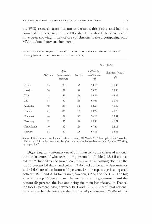
nationalism and changes in the income distribution 129
the WID research team has not understood this point, and has not launched a project to produce DI data. They should because, as we have been showing, many of the conclusions arrived comparing only MV tax data shares are incorrect.
table 2.17. oecd inequality reductions due to taxes and social transfers
in 2013 (survey data, working age population)
% of reduction
MV Gini
After
transfers before
taxes Gini
DI Gini
Explained by
social transfers
(a)
Explained by taxes
(b)
France .45 .33 .29 78.15 21.85
Sweden .38 .31 .28 70.20 29.80
USA .48 .43 .39 55.77 44.23
UK .47 .39 .35 68.64 31.36
Australia .42 .36 .32 58.58 41.42
Canada .41 .36 .33 59.22 40.78
Denmark .40 .29 .25 74.13 25.87
Germany .42 .35 .30 58.29 41.71
Netherlands .40 .32 .28 67.86 32.14
Norway .38 .30 .26 65.15 34.85
Source: OECD income distribution database consulted 20 March 2017, last updated 26 November 2016, retrieved from http://www.oecd.org/social/incomedistribution-database.htm, figure 4, “Working age population”.
Digressing for a moment out of our main topic, the shares of national income in terms of who uses it are presented in Table 2.18. Of course, column 2 divided by the sum of columns 2 and 3 is nothing else than the top 10 percent DI share, and column 3 divided by the same denominator is the DI share of the bottom 90 percent. On the top, usage is compared between 1910 and 2013 for France, Sweden, USA, and the UK. The big loser is the top 10 percent, and the winners are the government and the bottom 90 percent, the last one being the main beneficiary. In France, the top 10 percent loses, between 1911 and 2013, 29.7% of total national income; the beneficiaries are the bottom 90 percent with 72.4% of this

carlos obregón130
amount, and the government with the remaining 27.6%. In Sweden, the top 10 percent loses 22.6% of total national income, 54.9% of this goes to the bottom 90 percent, and 45.1% to the government. In the USA, the top 10 percent loses 9.1% of total national income, of which 57.1% goes to the bottom 90 percent, and 42.9% to the government. In the UK the top 10 percent loses 9.8% of total national income, the beneficiaries are the bottom 90% with the 64.9% of this amount, and the government with the remaining 35.1%.
table 2.18. usage1 of national income
1910 2013
G 10% 90% G 10% 90%
France 8.25 46.87 44.89 16.44 17.13 66.43
Sweden 7.89 40.01 52.10 18.08 17.40 64.51
USA 5.26 38.13 56.62 8.01 29.02 62.97
UK 8.97 33.27 57.77 12.38 23.50 64.11
1980 2013
G 10% 90% G 10% 90%
France 19.13 16.58 64.29 16.44 17.13 66.43
Sweden 23.38 10.79 65.83 18.08 17.40 64.51
USA 15.18 18.55 66.27 8.01 29.02 62.97
UK 17.22 16.45 66.32 12.38 23.50 64.11
Australia 19.89 14.02 66.09 11.49 17.70 70.82
Canada 24.26 18.29 57.46 16.26 23.51 60.23
Denmark 20.28 16.16 63.56 19.52 13.37 67.11
Germany 16.30 17.27 66.43 11.55 24.31 64.14
Netherlands 19.08 11.46 69.45 15.53 15.65 68.82
Norway 31.72 13.25 55.03 26.03 14.86 59.11
Source: Tni and Sni, same sources as Table 2.14.
1 Methodology: Tni-Sni is the usage of the government; (1 - government usage) * DI share=usage of top 10%; (1 - government usage) * (1 - DI share) = usage of 90%.
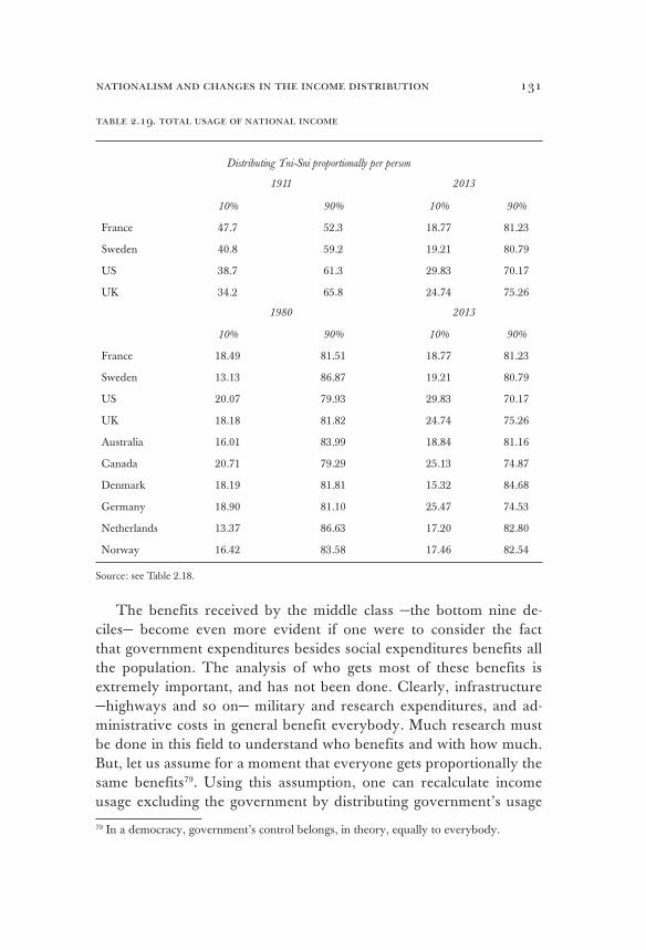
nationalism and changes in the income distribution 131
table 2.19. total usage of national income
Distributing Tni-Sni proportionally per person
1911 2013
10% 90% 10% 90%
France 47.7 52.3 18.77 81.23
Sweden 40.8 59.2 19.21 80.79
US 38.7 61.3 29.83 70.17
UK 34.2 65.8 24.74 75.26
1980 2013
10% 90% 10% 90%
France 18.49 81.51 18.77 81.23
Sweden 13.13 86.87 19.21 80.79
US 20.07 79.93 29.83 70.17
UK 18.18 81.82 24.74 75.26
Australia 16.01 83.99 18.84 81.16
Canada 20.71 79.29 25.13 74.87
Denmark 18.19 81.81 15.32 84.68
Germany 18.90 81.10 25.47 74.53
Netherlands 13.37 86.63 17.20 82.80
Norway 16.42 83.58 17.46 82.54
Source: see Table 2.18.
The benefits received by the middle class —the bottom nine de-ciles— become even more evident if one were to consider the fact that government expenditures besides social expenditures benefits all the population. The analysis of who gets most of these benefits is extremely important, and has not been done. Clearly, infrastructure —highways and so on— military and research expenditures, and ad-ministrative costs in general benefit everybody. Much research must be done in this field to understand who benefits and with how much. But, let us assume for a moment that everyone gets proportionally the same benefits79. Using this assumption, one can recalculate income usage excluding the government by distributing government’s usage
79 In a democracy, government’s control belongs, in theory, equally to everybody.
carlos obregón132
proportionally —that is ten percent to the top decile and ninety percent to the bottom nine deciles. In this case, income usage is the sum of the income usage in Table 2.18, plus the proportional benefits received through other government expenditures not included in social expen-ditures. The results are presented in Table 2.19.
The total usage share of the top 10 percent in national income us-age goes down in a similar fashion that its DI share. In France, the DI share falls, between 1910 and 2013, 30.5 percentage points (Table 2.14), and the total usage share falls 28.9 percentage points (Table 2.19). In Sweden the respective falls are 22.2 and 21.6; in the USA they are 9.7 and 8.9, and in the UK 8.7 and 9.5. Which confirms even further the relevance of using the DI shares and not the MV shares for long-term comparisons.
What have we learned up to here?1. That the top ten percent DI shares corresponding to the MV
shares reported in the WID data in 2013 are significantly smaller —between 21% to 35% for DI shares, versus between 30% to 46% for the MV share (Table 2.14).
2. In the last century, the redistribution in favor of the bottom 90 percent in DI share terms has been huge.
3. In France and Sweden, the top 10 percent DI share is less than half the value at the beginning of the century.
4. Even in the UK and the USA the top 10 percent DI share went down significantly, 27% and 22% respectively80.
The reality of the twentieth century is that the middle class —rep-resented by the bottom 90 percent— has benefited a lot. This is the consequence of democracies’ consolidation in all of these countries during this period. And it is a phenomenon of greater relevance in the political economic history of the World. The simple calculation we have presented, illustrates that doing long-term comparisons using MV income shares as Piketty and the WID do is misleading. Dissemi-nating to everybody the MV income shares —as the WID does— gen-erates a misleading image, both in term of levels and in the long-term direction of the income distribution.
80 Milanovic 2016, using survey data, shows a similar trend in the disposable Gini coef-ficient: for the UK it decreased more than 20%, and somewhat less in the US. Thus, it seems clear that the income distribution improved significantly during this period in both countries.

nationalism and changes in the income distribution 133
The within country income distribution 1980 to today
It is an undeniable fact that there has been an income concentration from 1980 to 2013 in many countries, particularly developed ones, as mea-sured by the top 10 percent’s share. From 1980 to today, the WID–tax data–MV share of the top 10 percent: goes up in twenty one countries, graph 2.2.a; is flat or just slightly up in six countries, graph 2.2.b; and goes down in two, graph 2.2.c.
GRAPH 2.2A. TOP 10% NATIONAL INCOME SHARE
Source: www.wid.word
Sh
are
of
tota
l (%
)
GRAPH 2.2B. TOP 10% NATIONAL INCOME SHARE
Source: www.wid.word
Shar
e of
tota
l (%
)
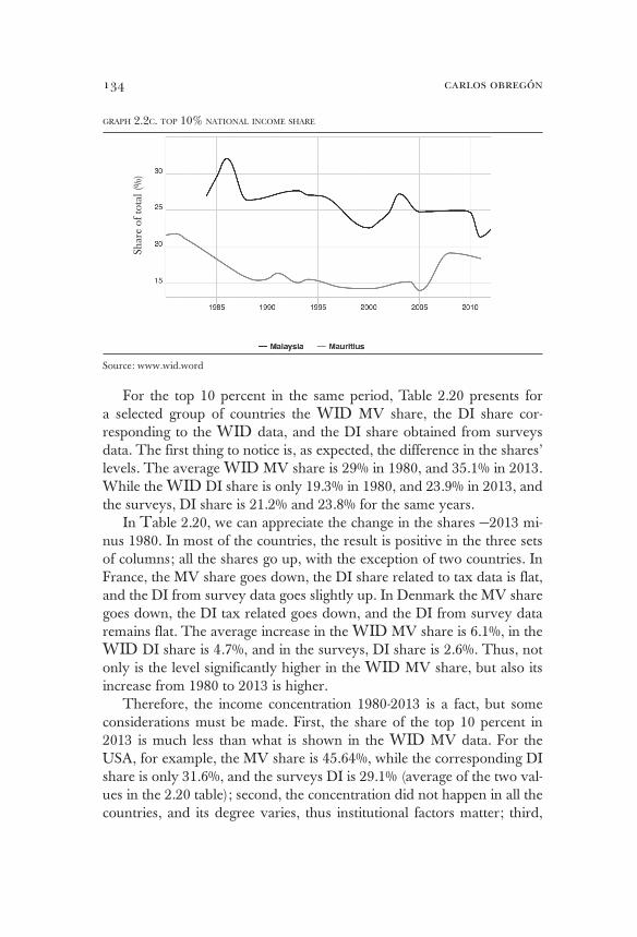
carlos obregón134
For the top 10 percent in the same period, Table 2.20 presents for a selected group of countries the WID MV share, the DI share cor-responding to the WID data, and the DI share obtained from surveys data. The first thing to notice is, as expected, the difference in the shares’ levels. The average WID MV share is 29% in 1980, and 35.1% in 2013. While the WID DI share is only 19.3% in 1980, and 23.9% in 2013, and the surveys, DI share is 21.2% and 23.8% for the same years.
In Table 2.20, we can appreciate the change in the shares —2013 mi-nus 1980. In most of the countries, the result is positive in the three sets of columns; all the shares go up, with the exception of two countries. In France, the MV share goes down, the DI share related to tax data is flat, and the DI from survey data goes slightly up. In Denmark the MV share goes down, the DI tax related goes down, and the DI from survey data remains flat. The average increase in the WID MV share is 6.1%, in the WID DI share is 4.7%, and in the surveys, DI share is 2.6%. Thus, not only is the level significantly higher in the WID MV share, but also its increase from 1980 to 2013 is higher.
Therefore, the income concentration 1980-2013 is a fact, but some considerations must be made. First, the share of the top 10 percent in 2013 is much less than what is shown in the WID MV data. For the USA, for example, the MV share is 45.64%, while the corresponding DI share is only 31.6%, and the surveys DI is 29.1% (average of the two val-ues in the 2.20 table); second, the concentration did not happen in all the countries, and its degree varies, thus institutional factors matter; third,
GRAPH 2.2C. TOP 10% NATIONAL INCOME SHARE
Source: www.wid.word
Sh
are
of
tota
l (%
)

nationalism and changes in the income distribution 135
the change in the concentration from 1980 to 2013 is higher in the MV data. In the USA, the top ten percent share increases in MV data 13.9 perceptual points versus 9.7 for the corresponding DI data, and 7.5 for survey data DI (using only WB data in Table 2.20); and fourth, as no-ticed in the previous section, the 1980-2013 income concentration must be understood as a consequence of the ICT revolution and in the context of the huge income de-concentration that happens between 1910-2013.
table 2.20. top 10% income share 1980-2014
Market value1
WID (MV)
Disposable income WID
(DI)Disposable income surveys2
1980 2013 1980 2013 1980 2013
Australia 24.20 30.09 17.50 19.9923.33 WB 26.53 WB
20.70 L 25.09 L
Canada 36.47 41.38 24.15 28.0724.33 WB 25.74 WB
21.11 L 24.26 L
Denmark 29.13 26.88 20.27 16.62 22.80 VG22.79 WB
21.00 L
France 31.11 29.81 20.50 20.50 24.80 L25.30 ES
26.84 WB
Germany31.36
38.95 20.64 27.49 20.31 L22.90 ES
(1983) 23.69 WB
Netherlands28.46
30.90 14.17 18.53 20.44 L21.30 ES
(1981) 22.57 WB
Norway 26.58 28.33 19.41 20.09 18.58 L19.60 ES
20.53 WB
Sweden 22.48 30.62 14.08 21.25 17.07 L 20.10 ES
USA 31.77 45.64 21.87 31.55 22.69 L30.19 WB
28.05 L
UK 28.37 41.29 19.88 26.83 20.68 L23.40 ES
26.80 L
x3 28.99 35.11 19.25 23.92 21.21 23.81

carlos obregón136
Sources of difference between MV WID and DI WID 2013
Sni t ≠ 1 s ≠ 1
Australia 48.45 32.26 19.29
Canada 61.17 31.03 7.80
Denmark 71.17 3.54 25.30
France 96.22 20.78 - 17.00
Germany 87.18 11.32 1.51
Netherlands 54.28 35.33 10.39
Norway 84.83 - 12.60 27.77
Sweden 85.85 0.00 14.15
USA 60.02 36.78 3.20
UK 63.15 24.74 12.11
Sources: columns 1 to 4 from WID database in the web, accessed 14 August 2017; last two columns from World Income Inequality Database (WIID), UNU-Wider, retrieved from https://www.wider.unu.edu/project/wild-world-income-inequality-database, WIID 3.4, 19 January 2017 excel file.
1 We have made the numbers between WID MV data and the DI surveys data as compatible as pos-sible. Therefore, not all years correspond to 1980-2013 because of data availability and the fact that it could not be fully compatible within two countries´ years. Considering that, years are as follows: Australia 1981-2010; Canada 1981-2010; Denmark 1976-2010; France 1978-2013; Germany 1983-2011, 1983 for the MV and 1981 for the DI surveys; Netherlands 1981-2012, 1981 for the MV and 1983 for the DI surveys; Norway 1979-2011; Sweden 1981-2013; USA 1979-2013; UK 1979-2013. Years for social expenditures: Australia 1980-2010; Canada 1980-2010, Denmark 1980-2010; France 1980-2013; Germany 1980-2010; Netherlands 1980-2013, Norway 1980-2010, Sweden 1980-2013,
USA 1980-2013; UK 1980-2013. Tax revenues years correspond to MV years.2 Disposable income surveys come from UN, same as Table 2.28. Eurostat (ES), World Bank (WB),
Luxembourg (L) and van Ginneken and Park (VG)
3 When two surveys for same year, average is calculated.
The critical question that remains is if the income distribution will or not continue its concentration trend in the future. Piketty’s 2014 book answer is that it will. As we have been shown, the data tendency is clearly insufficient to forecast statistically that such income concentration will happen —as far as the data is concerned, we just do not know. Piketty’s answer, however, is not statistically based —it is a theoretical answer. That is why in the next section we will review his theoretical argument, and we will show that there are no economic laws (or reasons) to expect a future income concentration. If it happens, it will be due to institutional and political factors. We cannot forecast —neither statistically or theoretically— it may or may not happen.
nationalism and changes in the income distribution 137
Before we move into the next section, we would like to do two things: 1. Analyze if there is any relationship between the income concen-
tration that has happened from 1980 to 2013 in the UK and the USA, and the middle class vote for Brexit and Mr. Trump.
2. We would like to compare the income distribution in devel-oped versus the developing economies.
why did people vote for brexit and mr. trump?
In an article of The Guardian in 2016, Piketty argues that the income concentration is to blame for the anger of the middle class shown in the votes in favor of Brexit and Donald Trump. Bourguignon 2015 makes a similar argument. Are they right?
Income distribution deterioration happened before the 2008 crisis. In fact, in 2008-2013 the share of the bottom 90% increased in the UK, and remained almost flat in the USA (see Table 2.21). Thus, the years in which there was income deterioration, mainly 1980-2008, people were not mad at the system. In addition, the years in which the 90% share remained flat or improved are the years where people did get mad. This seems to indicate that what made people mad was not the deterioration in the income distribution, but the 2008 crisis.
Between 1980-2008, considering the income distribution deterio-ration during these years, the GDP PPP per capita of the bottom 90% grew in the USA at an annual rate of 1.58% higher than the av-erage GDP per capita growth in France and Germany during these years; and in the UK, 2% similar to the average in the USA (see Ta-ble 2.22). Therefore, although their income share was going down, the middle class —the lower nine deciles— saw its income growing fast in 1980-2008, that is why they were not angry at the system then. With the crisis, between 2008-2013, the lowest 90% actually saw its share of income increasing very mildly in the USA, 1.8% (in relation to its 2008 share) and a significant 13.2% in the UK. But despite this improvement, they got mad at the system because their GDP per capita almost stagnated 2008-2013 in the USA, with an annual growth rate of only 0.13%, and grew very slowly in the UK, 0.61% in the same basis (see Table 2.22). This happened as house-holds were facing many other economic problems: they were losing

carlos obregón138
their houses, their financial assets, their good credit, and were facing high rates of unemployment. Unemployment went up, see Graph 2.3a and 2.3b. And it did significantly more for certain segments of the population, Graph 2.3b show that unemployment went up more than twice the average for people with basic education.
table 2.21. disposable income top 10% share (survey`s data)
1980 2008 2013
Australia
1981, 2008, 201023.33 WB 27.47 WB 26.53 WB
Canada
1981, 2007, 201024.33 WB 26.06 WB 27.54 WB
Denmark
1976, 2008, 201022.80 VG 21.70 WB 22.79 WB
France
1978, 2008, 201024.80 L 25.20 ES 25.30 ES
Germany
1981, 2008, 201120.31 L 24.30 ES 22.90 ES
Netherlands
1983, 2008, 201220.44 L 23.30 ES 21.30 ES
Norway
1979, 2008, 201118.58 L 21.10 ES 19.60 ES
Sweden
1980, 2008, 201317.07 L 19.80 ES 20.10 ES
USA
1980, 2007, 201322.69 L 30.73 WB 30.19 WB
UK
1980, 2008, 201320.68 L 26.80 ES 23.40 ES
Source and nomenclature: same as Table 2.20.
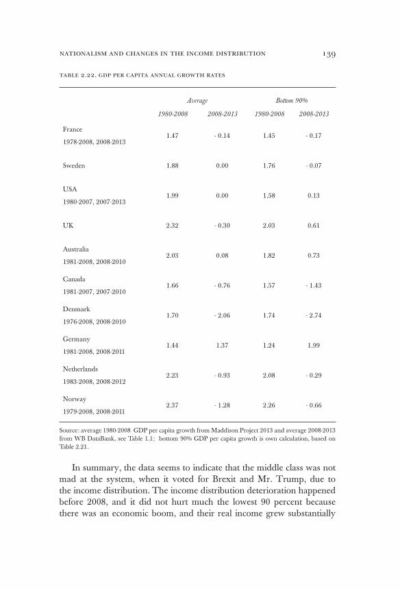
nationalism and changes in the income distribution 139
table 2.22. gdp per capita annual growth rates
Average Bottom 90%
1980-2008 2008-2013 1980-2008 2008-2013
France
1978-2008, 2008-20131.47 - 0.14 1.45 - 0.17
Sweden 1.88 0.00 1.76 - 0.07
USA
1980-2007, 2007-20131.99 0.00 1.58 0.13
UK 2.32 - 0.30 2.03 0.61
Australia
1981-2008, 2008-20102.03 0.08 1.82 0.73
Canada
1981-2007, 2007-20101.66 - 0.76 1.57 - 1.43
Denmark
1976-2008, 2008-20101.70 - 2.06 1.74 - 2.74
Germany
1981-2008, 2008-20111.44 1.37 1.24 1.99
Netherlands
1983-2008, 2008-20122.23 - 0.93 2.08 - 0.29
Norway
1979-2008, 2008-20112.37 - 1.28 2.26 - 0.66
Source: average 1980-2008 GDP per capita growth from Maddison Project 2013 and average 2008-2013 from WB DataBank, see Table 1.1; bottom 90% GDP per capita growth is own calculation, based on Table 2.21.
In summary, the data seems to indicate that the middle class was not mad at the system, when it voted for Brexit and Mr. Trump, due to the income distribution. The income distribution deterioration happened before 2008, and it did not hurt much the lowest 90 percent because there was an economic boom, and their real income grew substantially

carlos obregón140
despite the income distribution deterioration. The problem was the finan-cial 2008 crisis, which diminished dramatically the value of their assets, increased unemployment, and reduced almost to nothing the real growth rate of per capita GDP81.
81 An interesting question to research is: why, despite the fact that people were also mad in France and the Netherlands, the right wing did not win the election in these countries? I do not have the answer; there are cultural, institutional, and specific political considerations for each country that have to be addresed. A posible line of research might be linked to the capacity of the governments to provide protection during the crisis. France’s social expen-ditures are very high (see Table 2.13); the Netherlands, however, is similar to the UK. In 2014, both France and the Netherlands rank very high in the market value Gini reduction they achieved through taxes ad transfers, and the US and the UK Rank low (see Table 2.23 which can be found in the annex at the end of the book).
Source: World Development Indictors www.http://databank.worldbank.org
GRAPH 2.3A UNITED STATES
GRAPH 2.3B UNITED KINGDOM
Source: World Development Indictors www.http://databank.worldbank.org
Unemployment, total
(% of total labor force) (national estimate)
Unemployment with basic education
(% of total labor force with basic education)
Unemployment, total (% of total labor force) (national estimate)
nationalism and changes in the income distribution 141
income distribution: developed versus developing countries
In tables 2.24, 2.25, and 2.26, we can appreciate the relationship between GDP per capita (in 2011 PPPs) and the Gini coefficients. Notice that there is not a simple relationship between the income level and the in-come distribution, neither between regions nor between countries. Mid-dle East and North Africa, with a GDP per capita of 11,939 (2011 con-stant international dollars), had a similar level of development that Latin America and the Caribbean, with a GDP per capita of 10,308, in 1993 (see Table 2.25). Despite this, inequality was much higher in the second region with a 0.49 Gini versus 0.398 in the first. The 0.339 Gini in 1993 of Eastern Europe and Central Asia is similar to the 0.31 Gini of South Asia or the 0.314 Gini of industrialized economies, except that the GDP per capita are very different: 19,367 dollars for the first region, 1,950 for the second, and 30,090 for the third. Latin America and Caribbean, and Sub-Saharan Africa have very high and similar Ginis, 0.49 and 0.476 respectively despite their very different income levels, 10,308 and 2,315.
The effect of economic growth in the Ginis is not clear. East Asia Pacific grew more rapidly than the World, 4.5%, between 1993 to 2008 (Table 2.25), versus 2.46%; and its Gini went up, while the World’s went down. Then, it again grew faster from 2008-2013, 5.14% versus 1.86%, and its Gini went down, while the World’s remained almost flat.
Sub-Saharan Africa and China had a similar GDP per capita in 1993, 2,315 versus 2,090. As China developed, its GDP per capita went to 11951 in 2013, and its Gini went up from 0.355 in 1993 to 0.422 in 2013, as one would expect with Kuznets’ income distribution theory. Sub-Saharan Afri-ca did not develop much, its GDP per capita went up only to 3,391, and its Gini went down from 0.476 to 0.438, not expected with Kuznets’ theory. Moreover, China in 2013 with a much higher GDP per capita has a lower Gini in 2013 (0.422) than the Gini of Sub-Saharan Africa both in 1993 (0.476), and in 2013 (0.438). India in 2013 has a GDP per capita of 4,636 higher than Sub-Saharan Africa, and a much lower Gini of only 0.352.
The industrialized economies have a very low Gini of 0.318 in 2013, which shows good governance, but India has a Gini of only 0.352, and Eastern Europe and Central Asia of 0.314. Therefore, it is very difficult to refer to income categories or development stages related to the income distribution because there are so many counterexamples one just must recognize they seem to be the rule.
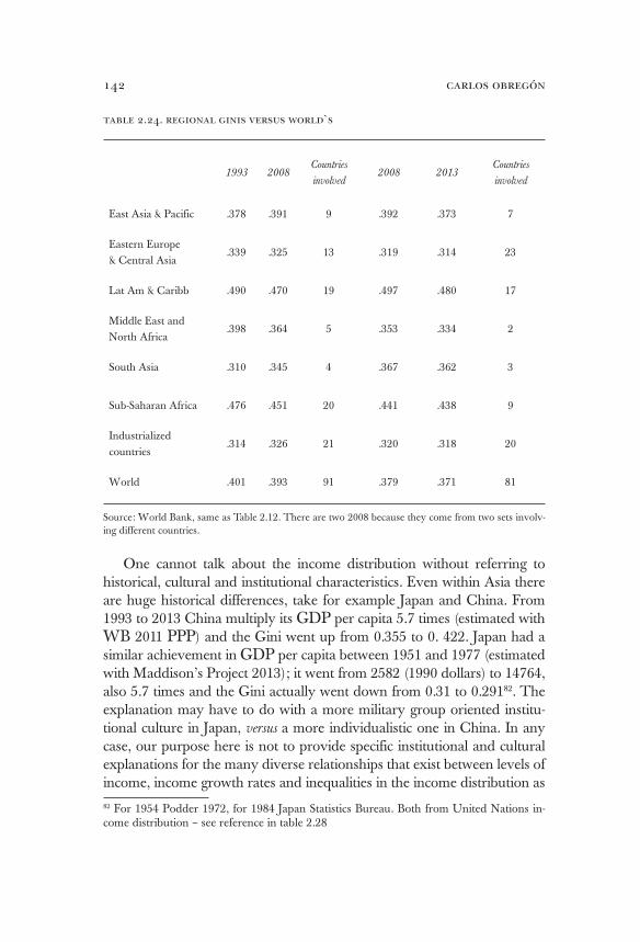
carlos obregón142
table 2.24. regional ginis versus world`s
1993 2008
Countries
involved2008 2013
Countries
involved
East Asia & Pacific .378 .391 9 .392 .373 7
Eastern Europe & Central Asia
.339 .325 13 .319 .314 23
Lat Am & Caribb .490 .470 19 .497 .480 17
Middle East and North Africa
.398 .364 5 .353 .334 2
South Asia .310 .345 4 .367 .362 3
Sub-Saharan Africa .476 .451 20 .441 .438 9
Industrialized countries
.314 .326 21 .320 .318 20
World .401 .393 91 .379 .371 81
Source: World Bank, same as Table 2.12. There are two 2008 because they come from two sets involv-ing different countries.
One cannot talk about the income distribution without referring to historical, cultural and institutional characteristics. Even within Asia there are huge historical differences, take for example Japan and China. From 1993 to 2013 China multiply its GDP per capita 5.7 times (estimated with WB 2011 PPP) and the Gini went up from 0.355 to 0. 422. Japan had a similar achievement in GDP per capita between 1951 and 1977 (estimated with Maddison’s Project 2013); it went from 2582 (1990 dollars) to 14764, also 5.7 times and the Gini actually went down from 0.31 to 0.29182. The explanation may have to do with a more military group oriented institu-tional culture in Japan, versus a more individualistic one in China. In any case, our purpose here is not to provide specific institutional and cultural explanations for the many diverse relationships that exist between levels of income, income growth rates and inequalities in the income distribution as 82 For 1954 Podder 1972, for 1984 Japan Statistics Bureau. Both from United Nations in-come distribution – see reference in table 2.28
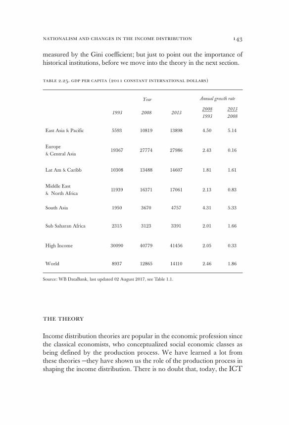
nationalism and changes in the income distribution 143
measured by the Gini coefficient; but just to point out the importance of historical institutions, before we move into the theory in the next section.
table 2.25. gdp per capita (2011 constant international dollars)
Year Annual growth rate
1993 2008 20132008
1993
2013
2008
East Asia & Pacific 5593 10819 13898 4.50 5.14
Europe & Central Asia
19367 27774 27986 2.43 0.16
Lat Am & Caribb 10308 13488 14607 1.81 1.61
Middle East & North Africa
11939 16371 17061 2.13 0.83
South Asia 1950 3670 4757 4.31 5.33
Sub Saharan Africa 2315 3123 3391 2.01 1.66
High Income 30090 40779 41456 2.05 0.33
World 8937 12865 14110 2.46 1.86
Source: WB DataBank, last updated 02 August 2017, see Table 1.1.
the theory
Income distribution theories are popular in the economic profession since the classical economists, who conceptualized social economic classes as being defined by the production process. We have learned a lot from these theories —they have shown us the role of the production process in shaping the income distribution. There is no doubt that, today, the ICT

carlos obregón144
revolution explains most of the income distribution tendencies that we observe, both nationally and globally. However, in their specific fore-casts, all the income distribution theories turned out to be wrong. The Stationary State of the classical economists never happened, Marx’s fall-ing rate of profit did not occur, Kuznet’s theory did not predict the in-come concentration that we have recently observed in many developed countries. I have shown why Piketty’s long-term laws are wrong83, and Milanovic’s recent attempt to reconstruct the Kuznet’s theory as Kuznets Waves, as we will argue later on, can also be counted as a failure. Why?
The reason —among others— is that the production process involves technologies and these change through innovation, and innovation cannot be predicted or forecasted (in fact most exogenous shocks cannot be fore-casted either). As Karl Popper said, innovation is about what we do not know. New technologies always come as a surprise. They define new modes of production that put pressure for new institutions to emerge, and for new ways to redistribute income. But, there is also social engineering, which is as well subject for innovation. Thus, each culture and society adapts to the new technological changes in a specific institutional way of its own.
In what follows, we will describe each one of the main income distri-bution theories and we will explain why they failed. In doing so, we must remind the reader that, despite being unable to forecast the future or a common pattern that all the societies have to follow, these theories have been very helpful in discovering many of the pressures involved in the income distribution’s determination. Therefore, they are useful for our understanding, both of the potential causes of income redistributions and of how the social engineering should respond to them.
The classical economists
The classical economists income distribution theory is shown in Table 2.27, and it actually is conducive to a Stationary State. In summary, more agricultural production implies diminishing returns through the usage of less productive land, which implies that rent in the more productive lands goes up —rentiers income goes up; food becomes more expensive, nominal salaries go up, but real salaries go down in the long run to the subsistence level —worker’s income goes to subsistence levels; and there-83 Obregon, 2015: Piketty is Wrong
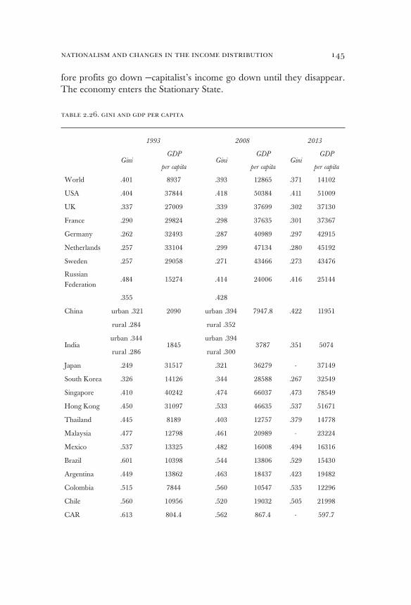
nationalism and changes in the income distribution 145
fore profits go down —capitalist’s income go down until they disappear. The economy enters the Stationary State.
table 2.26. gini and gdp per capita
1993 2008 2013
GiniGDP
per capitaGini
GDP
per capitaGini
GDP
per capita
World .401 8937 .393 12865 .371 14102
USA .404 37844 .418 50384 .411 51009
UK .337 27009 .339 37699 .302 37130
France .290 29824 .298 37635 .301 37367
Germany .262 32493 .287 40989 .297 42915
Netherlands .257 33104 .299 47134 .280 45192
Sweden .257 29058 .271 43466 .273 43476
Russian Federation
.484 15274 .414 24006 .416 25144
China
.355
2090
.428
7947.8 .422 11951 urban .321 urban .394
rural .284 rural .352
Indiaurban .344
1845urban .394
3787 .351 5074rural .286 rural .300
Japan .249 31517 .321 36279 - 37149
South Korea .326 14126 .344 28588 .267 32549
Singapore .410 40242 .474 66037 .473 78549
Hong Kong .450 31097 .533 46635 .537 51671
Thailand .445 8189 .403 12757 .379 14778
Malaysia .477 12798 .461 20989 - 23224
Mexico .537 13325 .482 16008 .494 16316
Brazil .601 10398 .544 13806 .529 15430
Argentina .449 13862 .463 18437 .423 19482
Colombia .515 7844 .560 10547 .535 12296
Chile .560 10956 .520 19032 .505 21998
CAR .613 804.4 .562 867.4 - 597.7

carlos obregón146
Botswana .490 8427 .605 13768 - 15568
South Africa .593 9014 .630 12197 .634 12446
Cameroon - 2248 .428 2664 .465 2815
Kenya .445 2184 .485 2335 - 2683
Congo Rep - 4928 .473 4730 .489 5317
Source: GINIs United Nations, same as Table 2.20; GDP per capita WB DataBank, updated 02 August 2017, see Table 1.1.
There is no room for the capitalists’ profits, because if they increase, the subsistence salary will go down, and population will go down di-minishing the labor supply and increasing the salary again to the subsis-tence level. For Smith, it was key to avoid the Stationary State, which was a natural long run tendency, and for that, capitalism has to be expanding, that is why trade and enlarging the markets was so cru-cial, because larger markets fostered mass production and allowed for the technological innovations needed to maintain capitalism expanding (Smith actually was right, because this is what actually happened later on in Capitalism).
table 2.27. classical economists´ income distribution theory
Higher agricultural production
Diminish-ing returns
despite technological advancements
Less productive land used (rent
goes up)
More expen-sive food (sal-ary goes up)
Profits go down despite technological
improvements in manufactures
MALTHUS
Population grows geometricallyProfits go down and salary becomes a salary of subsistence
Food arithmetically Policy reduce population growth
RICARDO
Points out technological advances but argues that they are not enough
Policy import food
Classes: rent goes upRenter´s income increase, nominal salary goes up but real goes down
Profits down - Capitalists Workers to subsistance level
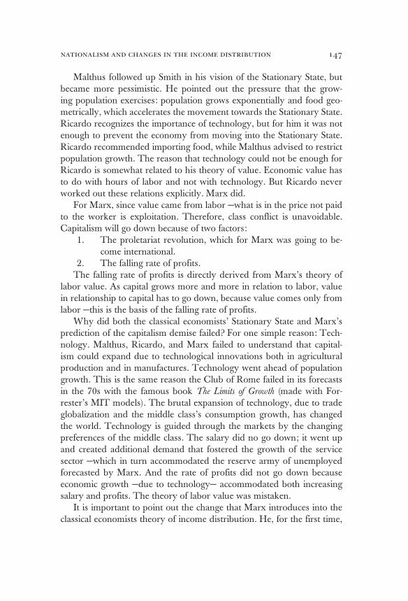
nationalism and changes in the income distribution 147
Malthus followed up Smith in his vision of the Stationary State, but became more pessimistic. He pointed out the pressure that the grow-ing population exercises: population grows exponentially and food geo-metrically, which accelerates the movement towards the Stationary State. Ricardo recognizes the importance of technology, but for him it was not enough to prevent the economy from moving into the Stationary State. Ricardo recommended importing food, while Malthus advised to restrict population growth. The reason that technology could not be enough for Ricardo is somewhat related to his theory of value. Economic value has to do with hours of labor and not with technology. But Ricardo never worked out these relations explicitly. Marx did.
For Marx, since value came from labor —what is in the price not paid to the worker is exploitation. Therefore, class conflict is unavoidable. Capitalism will go down because of two factors:
1. The proletariat revolution, which for Marx was going to be-come international.
2. The falling rate of profits. The falling rate of profits is directly derived from Marx’s theory of
labor value. As capital grows more and more in relation to labor, value in relationship to capital has to go down, because value comes only from labor —this is the basis of the falling rate of profits.
Why did both the classical economists’ Stationary State and Marx’s prediction of the capitalism demise failed? For one simple reason: Tech-nology. Malthus, Ricardo, and Marx failed to understand that capital-ism could expand due to technological innovations both in agricultural production and in manufactures. Technology went ahead of population growth. This is the same reason the Club of Rome failed in its forecasts in the 70s with the famous book The Limits of Growth (made with For-rester’s MIT models). The brutal expansion of technology, due to trade globalization and the middle class’s consumption growth, has changed the world. Technology is guided through the markets by the changing preferences of the middle class. The salary did no go down; it went up and created additional demand that fostered the growth of the service sector —which in turn accommodated the reserve army of unemployed forecasted by Marx. And the rate of profits did not go down because economic growth —due to technology— accommodated both increasing salary and profits. The theory of labor value was mistaken.
It is important to point out the change that Marx introduces into the classical economists theory of income distribution. He, for the first time,
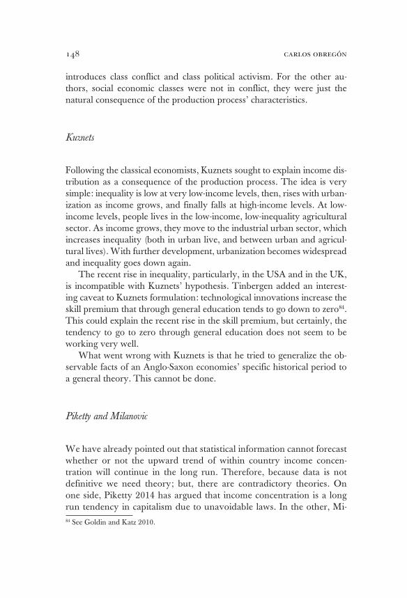
carlos obregón148
introduces class conflict and class political activism. For the other au-thors, social economic classes were not in conflict, they were just the natural consequence of the production process’ characteristics.
Kuznets
Following the classical economists, Kuznets sought to explain income dis-tribution as a consequence of the production process. The idea is very simple: inequality is low at very low-income levels, then, rises with urban-ization as income grows, and finally falls at high-income levels. At low-income levels, people lives in the low-income, low-inequality agricultural sector. As income grows, they move to the industrial urban sector, which increases inequality (both in urban live, and between urban and agricul-tural lives). With further development, urbanization becomes widespread and inequality goes down again.
The recent rise in inequality, particularly, in the USA and in the UK, is incompatible with Kuznets’ hypothesis. Tinbergen added an interest-ing caveat to Kuznets formulation: technological innovations increase the skill premium that through general education tends to go down to zero84. This could explain the recent rise in the skill premium, but certainly, the tendency to go to zero through general education does not seem to be working very well.
What went wrong with Kuznets is that he tried to generalize the ob-servable facts of an Anglo-Saxon economies’ specific historical period to a general theory. This cannot be done.
Piketty and Milanovic
We have already pointed out that statistical information cannot forecast whether or not the upward trend of within country income concen-tration will continue in the long run. Therefore, because data is not definitive we need theory; but, there are contradictory theories. On one side, Piketty 2014 has argued that income concentration is a long run tendency in capitalism due to unavoidable laws. In the other, Mi-84 See Goldin and Katz 2010.
nationalism and changes in the income distribution 149
lanovic 2016 defends cycles that he has called the Kuznets waves. For this second author inequality goes up and down, and up and down, and so on. Who is right? Can we really construct a theory of the income distribution?
Piketty tells us that there are long-term laws that will increase within country inequality, and that between countries inequality will go down significantly —because he sees a very quick convergence from other coun-tries to the West’s quality of life. Thus, for him the world’s key problem is the upward trend of within country inequality. We will argue that Piketty is wrong, as we had been doing before. Milanovic on the other side, sees the United States and the UK approaching the peak of within country inequality, so these countries will start the descending phase of the cycle. We will argue that Milanovic’s Kuznets waves theory lacks any power of prediction.
To judge who is right not only involves a theoretical scrutiny of their thesis, it also requires a discussion of: what is economic theory all about? Do markets define an economic equilibrium by themselves? Or do the markets need an institutional arrangement to function properly? If the answer is no to the first question, and yes to the second, then one has to recognize that the economic equilibrium is the outcome of both the unstoppable market forces and the decisive institutional framework that defines their operation.
Piketty’s laws have in common with classical and neoclassical eco-nomics the believe that there are general market laws that define the eco-nomic relations between individual agents. But this assumption has been proven again and again as theoretically wrong. Whether one looks at informational economics, at institutional economics or at Nash’s theory the undeniable fact is that there are multiequilibria, and that many of them are not pareto optimums.
The institutional arrangement provides information, laws, and insti-tutions that regulate markets, make them feasible, and provides the re-quired certainty for markets to operate. Knight and Keynes had already warned us that markets did not operate well with uncertainty, and that institutions were required to reduce it. But it is not until contemporary economics that multiequilibria are mathematically derived, and that the non-pareto Nash equilibriums were formalized. Against this background, at-tempts to derive the income distribution from market’s necessary laws are awkward, and it is not surprising that when the theoretical work that sustains them is carefully analyzed, it turns out to be wrong.

carlos obregón150
Piketty
Why is he wrong? Piketty is wrong because he confuses wealth and capi-tal. We do have an economic theory of capital, but not one of wealth. The distribution of wealth is not defined by the factors of production, like Piketty has argued. Capital is an input in the production process, and as such it is subject to the long run logic of the markets. Wealth is driven by medium-term economic waves which are technologically and institution-ally driven. Let us look specifically at: where is Piketty wrong? In a recent technical article —which I recommended to the interested reader— I have shown why Piketty is wrong85. In here, I will only summarize some of the arguments presented there to use them for our present discussion. Piketty confuses wealth with capital, and in doing so he creates confusion as to how the economic markets operate. He uses a midwave income concentration produced by the ICT technological revolution to forecast a world’s long-term income concentration; he goes as far as to defend long-term income concentration laws in capitalism. For Piketty, economic world’s growth will slow down. Therefore, with a more or less rigid sav-ings rate, capital income ratio goes up. And with a relatively rigid rate of return on capital, the capital share of income goes up. Since the owner-ship of capital is concentrated, income concentration does occur.
To understand what is wrong, one needs to take two steps. First, explain: where does the statistical factual increase in wealth comes from, and show that it is not a long-term, but a medium-term phenomenon, and because of economic reasons, eventually it will go away. It will become a cycle. Although, we cannot forecast the size or durability of such cycles. Second, explain: how to make compatible the medium-term increase in wealth with the literature on both the elasticity of capital and the behavior of the savings rates in dynamic growth models. Both steps have to rec-ognize one simple economic fact: markets are flexible and they do work —price rigidities do not make sense.
In the mentioned article, we identified the wealth increase with medi-um-term waves happening in the real estate and the stock markets. We have shown that if these phenomena are taking away all the statistics are compatible with the 75-year literature on the capital- labor elasticity for all the countries involved, Table 2.5 and 2.6 of the mentioned article show these results. Capital is not wealth. The return rate in capital is flexible, and
85 Obregon 2015.
nationalism and changes in the income distribution 151
it is subject to the diminishing returns law. Wealth increases do not mean capital increases. The medium-term rate of return on wealth may remain high; but that does not mean that the return on capital also remains high.
The medium-term boom in real estate and the stock market is pro-duced by the ICT revolution which: 1) increases companies’ expected profits due to the increase in productivity, and 2) increases the demand of urban real estate because of urban located manufacturing services com-panies, and the associated boom in the financial sector that increases the number of executives in this sector and their relative salaries. But eventu-ally both phenomenon have a market logic of their own: stock markets in a stationary state —in the long run— have to be governed by book value, and real state prices by reposition costs. Therefore, the medium-term price increase in both markets do produce wealth and income concentra-tion, but it is not a long-term phenomenon —it cannot be used to establish long-term economic laws, neither to forecast the next century.
A higher saving rate does move the economy from one inferior growth path to another superior one; they are both parallel to one another, but in the superior one the output per capita is higher. There has to be a re-lationship between the saving rate and the growth rate of the economy. Dynamic economic models have shown that there is one.
Using both a flexible rate of return in capital and a flexible savings rate, we have constructed alternative forecast to Piketty’s, which behave well according to both the dynamic growth models that define the sav-ings rate, and the seventy-five years of literature in capital labor elasticity. Table 5.1 of the mentioned article shows these results.
Thus, there are no long-term laws, not even a forecastable long run tendency for income concentration. Piketty is wrong. But the medium-term wealth increases produced by the ICT revolution are there, as well as their income distribution consequences. This implies that some income redistribution policies should be recommended; we will be doing so in chapter five.
Milanovic
Milanovic 2016 argues that there are inequality waves —that he calls Kuznets waves— both in preindustrial societies —where the mean income does not grow, and in industrial societies —where the mean income grows.

carlos obregón152
In preindustrial societies, the general idea is similar to the Stationary State of the classical economists. Rent is defined by the marginal productivity of the least productive land. Inequality is given by the land rent —subsistence salary ratio, which is stable. In addition, inequality goes up or down, only temporarily, by exogenous shocks such as epidemics, war or trade.
In preindustrial societies, inequality goes down because:1. Events that reduce the supply of labor, increase wages, and
reduce inequality. Amongst these events, we find: a) epidem-ics like the Plague or Black Death, and b) war because of the demand for soldiers.
2. Events that destroy capital or required higher taxes from the rich, such as wars.
Also, inequality goes up when there are temporary increases in mean income that generate a surplus that can go to capitalist’s profits. Due to the surplus, capitalist’s profits can increase without bringing the salary below the subsistence level. Such temporary increases in mean income may be consequence of positive trade shocks such as the discovery of the Americas or the new trade routes with Asia, conquered territories that provide a premium over war expenses, or positive production shocks. Milanovic cites, for example, a period of increase wood production in Spain. Thus, as mean income increase in preindustrial societies, it pro-vides space for inequality to go up, and as the economic surplus goes down inequality has to go down, because societies are moving back to the Classical economists’ Stationary State. Milanovic cites the case of Rome, whose Gini was around 0.41 in the mid second century, and as Rome falls it gets to be around 0.15-0.16 in the year 700.
In industrial societies, technology positive shocks create the necessary surplus for inequality to increase. Both urban inequality and urban-agri-cultural inequality go up. Inequality goes down because of:
1. Wars —through destruction and higher taxation.2. Civil conflict (state breakdown). 3. Social pressure through politics (socialism, welfare state, trade
unions). 4. Widespread education.5. Aging population (demand for social protection).6. Technological change that favors low-skilled workers (of which
we have not seen much).Milanovic points out that diverse societies respond institutionally dif-
ferent to the economic forces described above, but he insists that institu-

nationalism and changes in the income distribution 153
tions are endogenous —in the sense that they can only act within the mar-gin that the income level allows them. The income distribution for him is the result of the interplay between economic and institutional forces.
Milanovic provides several examples of the so-called Kuznets waves. Let us review first the USA’s wave (see Table 2.29). The Gini goes up from 0.441 in 1774 to around 0.50 in 1933, then goes down until 0.35 after Second World War and remains there until 1979 when it bottoms down, and afterwards starts increasing until 2013, when its is around .040. We can see the Kuznets waves in here right away. From 1774 to 1933, the Gini go up and then go down from 1933 to 1979 jus as Kuznets forecasted, and then go up again producing the wave, which Kuznets did not forecast. What happened was that the Gini increased again after 1979. What was against Kuznets forecast? The ICT revolution.
In here, we can already appreciate the most important limitation of the Kuznets waves. They lack predictive power —because all the forces that Milanovic mentions, cannot be forecasted. If the ICT revolution had not happened, the Gini would have remained low because salaries in the man-ufacturing sector in the USA would have remained high, and because the increase in executive salaries associated with the ICT revolution would not have happened, nor the stock market and real estate booms.
The world changes as a result of exogenous shocks that cannot be forecasted. Therefore, we know that there are exogenous forces that push inequality up and down. Describing them is important, and in that Mi-lanovic has had a very important contribution –—we have learned a lot from him. But, that does not mean that we can forecast the future.
Moreover, much has to be done to understand the interplay between institutional and economic forces. To do that, we need to understand the institutional history of each country or region. There is not a straight for-ward relation between the level of income and the income distribution. It is true that low-income levels restrict the possibility of inequalities, in the sense of the classical economist Stationary State. If there is no surplus there cannot be inequality. However, it is not true that once a surplus is created inequality will necessarily go up, and it is even less true that if it goes up we can forecast the path that it will take. There are just too many possibilities that depend in the particular institutional and historical background of each country. One must look at economic forces as exercising pressures, which may define in many cases the direction that inequality will follow. But the end result of what will happen with the income distribution —the Gini level that it will take— is not known and cannot be forecasted.
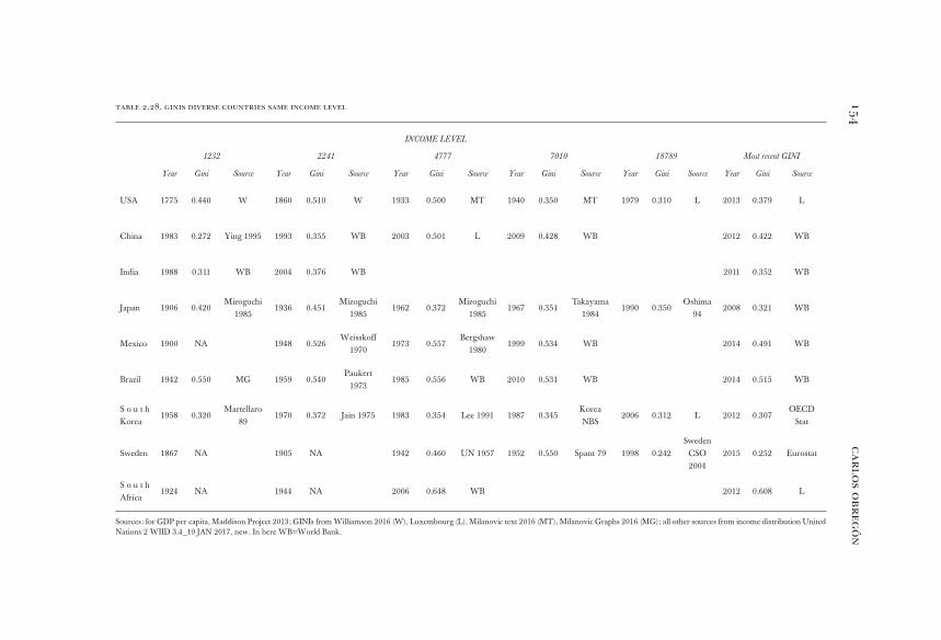
ca
rlo
s o
br
eg
ón
15
4
table 2.28. ginis diverse countries same income level
INCOME LEVEL
1232 2241 4777 7010 18789 Most recent GINI
Year Gini Source Year Gini Source Year Gini Source Year Gini Source Year Gini Source Year Gini Source
USA 1775 0.440 W 1860 0.510 W 1933 0.500 MT 1940 0.350 MT 1979 0.310 L 2013 0.379 L
China 1983 0.272 Ying 1995 1993 0.355 WB 2003 0.501 L 2009 0.428 WB 2012 0.422 WB
India 1988 0.311 WB 2004 0.376 WB 2011 0.352 WB
Japan 1906 0.420Mizoguchi
19851936 0.451
Mizoguchi 1985
1962 0.372Mizoguchi
19851967 0.351
Takayama 1984
1990 0.350Oshima
942008 0.321 WB
Mexico 1900 NA 1948 0.526Weisskoff
19701973 0.557
Bergshaw 1980
1999 0.534 WB 2014 0.491 WB
Brazil 1942 0.550 MG 1959 0.540Paukert
19731985 0.556 WB 2010 0.531 WB 2014 0.515 WB
S o u t h Korea
1958 0.320Martellaro
891970 0.372 Jain 1975 1983 0.354 Lee 1991 1987 0.345
Korea NBS
2006 0.312 L 2012 0.307OECD
Stat
Sweden 1867 NA 1905 NA 1942 0.460 UN 1957 1952 0.550 Spant 79 1998 0.242Sweden
CSO 2004
2015 0.252 Eurostat
S o u t h Africa
1924 NA 1944 NA 2006 0.648 WB 2012 0.608 L
Sources: for GDP per capita, Maddison Project 2013; GINIs from Williamson 2016 (W), Luxembourg (L), Milanovic text 2016 (MT), Milanovic Graphs 2016 (MG); all other sources from income distribution United Nations 2 WIID 3.4_19 JAN 2017, new. In here WB=World Bank.
nationalism and changes in the income distribution 155
Table 2.28 shows Ginis coefficients for diverse countries at the same level of GDP per capita. We can see that modernization from a GDP per capita of 1,232 to 2,241 (1,990 PPP dollars) did imply the Gini to rise in all these examples, thus there is no doubt that there are economic pres-sures, and that the Kuznets story is there as a background pressuring the direction the Gini will follow86.
But the story evolves very differently in each case. It happens at very different levels of inequality defined by institutional and historical spe-cific factors in each case. At 2,241 dollars, there is a very wide range of Ginis from 0.54 in Brazil to 0.355 in China. Thus, there is no doubt that institutional factors are the decisive ones in the end result —as far as the inequality level is concerned. As modernization happens differently, countries experienced it in a different way. With the GDP per capita go-ing from 2,241 to 18,789, the direction of the Gini is defined by economic pressures in the Kuznets sense in the USA, Japan, and South Korea —in all cases the Gini goes down. But, how much does it go down? That is de-fined by historical and institutional forces. In USA, the Gini goes down a lot, 0.2, in Japan half of this, 0.1, and in South Korea only 0.06, less than one third the fall in the US.
However, even the Gini’s direction is not necessarily defined by eco-nomic pressures. Take the modernization from 2,241 dollars to 7,010 dollars as an example; in some countries, the Gini goes down, and in others, it goes up. In China, Mexico, and Brazil the Gini goes up as predicted by Kuznets; but in the USA, Japan, and South Korea the Gini goes down. In China it went up 0.146, in Mexico it went up 0.031, and in Brazil 0.016. While in USA the Gini goes down 0.16, in Japan 0.05, and in South Korea 0.018. If we take the modernization from 7,010 dollars to 18,789 dollars, USA’s Gini goes down 0.04, Japan is flat, and Sweden goes down a lot, 0.308.
It could be argued that we are taking very reduced income changes, that we must look at the whole country’s income history. But even if one does that, the picture is still dominated by institutional and histori-cal factors. There seems to be different long run Gini levels in different countries —Gini differences that seem independent of the income levels, and that seem to reflect diverse institutional historical characteristics.
Table 2.29, presents the history of the Gini’s for selected countries. USA inequality has remained very constant at around 0.4 (0.41 is the average of all the historical points reported in the table). 1774 to 2013,
86 In here, for the GDP per capita, we are using the Maddison 2013 Project, which is the same one used by Milanovic 2016.

carlos obregón156
the Gini goes from 0.441 to 0.39587. UK has a similar inequality history than the USA (its average of the points reported is 0.39), but lately insti-tutional policies have brought inequality down to European standards. 1688 to 2013 the Gini goes from 0.45 to 0.326. In Germany, inequality has historically been lower than in USA or the UK (the average of the points reported is 0.31), and it has been around today’s level of 0.3. 1882 to 2015, the Gini goes from 0.34 to 0.307. The Netherlands started as an unequal country as much as the USA or the UK, but institutional poli-cies have brought the Gini substantially down (the average of the points reported is 0.35 versus a level of around 0.25 -0.26 since the 80s). 1561 to 2015, the Gini goes from 0.55 to 0.264. Italy also started as an unequal country, and has become more equal as it modernizes (the average of the points reported is 0.37 versus actual level of 0.32), but it is less egalitarian than the Netherlands. 1861 to 2015, the Gini goes from 0.51 to 0.324. Spain has had a fairly stable history of inequality (the average of the points reported is 0.36 versus today’s level of 0.36). 1850 to 2013, the Gini goes from 0.38 to 0.359. Japan was always more egalitarian than other countries in the West, and it has had a fairly stable history of inequality (average of the points reported is 0.35 versus today’s 0.32). 1895 to 2011, the Gini goes from 0.42 to 0.32. Brazil and Chile had been traditionally very unequal countries (the average of the points reported for both is 0.52 versus today’s 0.52 for Brazil, and 0.51 for Chile). In Brazil, 1850 to 2014, the Gini goes from 0.48 to 0.515. In Chile, 1850 to 2013, it goes from 0.53 to 0.505. Right away, we can see that there are long run histori-cal institutional characteristics that differentiate the countries.
table 2.29. historical ginis (selected countries)
Year Gini Source Year Gini Source
USA UK
1774 0.441 W 1688 0.450 MG
1860 0.510 W 1867 0.575Collete 2000
(UN)
1933 0.500 MT 1913 0.500 MT
1947 0.350 MT 1938 0.380 UN 1957
87 Average of the two reports for 2013 in Table 2.29.

nationalism and changes in the income distribution 157
1974 0.359 L 1963 0.300 MT
1979 0.310 L 1979 0.267 L
2010
0.369 L 1995 0.346 L
0.405 WB2010
0.337 L
0.400 MT 0.348 WB
20130.379 L
20130.332 L
0.411 WB 0.326 WB
=40.59 x=38.77
SPAIN ITALY
1850 0.380 MG 1861 0.510 MG
1953 0.540 MG & MT 1931 0.850 MG
1965 0.320Statistical yearbook
1948 0.420 Brandolini
1980 0.300 L 1982 0.310 Brandolini
1985 0.300 MG 1983 0.300 MG
1995 0.356 L 1986 0.309 L
20100.333 L 1998 0.351 L
0.358 WB2010
0.328 L
20130.343 L 0.317 Eurostat
0.359 WB 2015 0.324 Eurostat
x=36.16 x=36.63
GERMANY NETHERLANDS
1882 0.340 MG 1561 0.550 MG
1913 0.320 MG 1914 0.500 MG
1950 0.396 Brandolini 1962 0.420 MG
1962 0.390 MG 1962 0.440 UN 1957
1973 0.300 L 1983 0.252 L
1978 0.264 L 1999 0.231 L
1981 0.255 Brandolini 2010 0.257 L
2010 0.288 L 2013 0.264 L
2013 0.295 L 2015 0.264 Eurostat
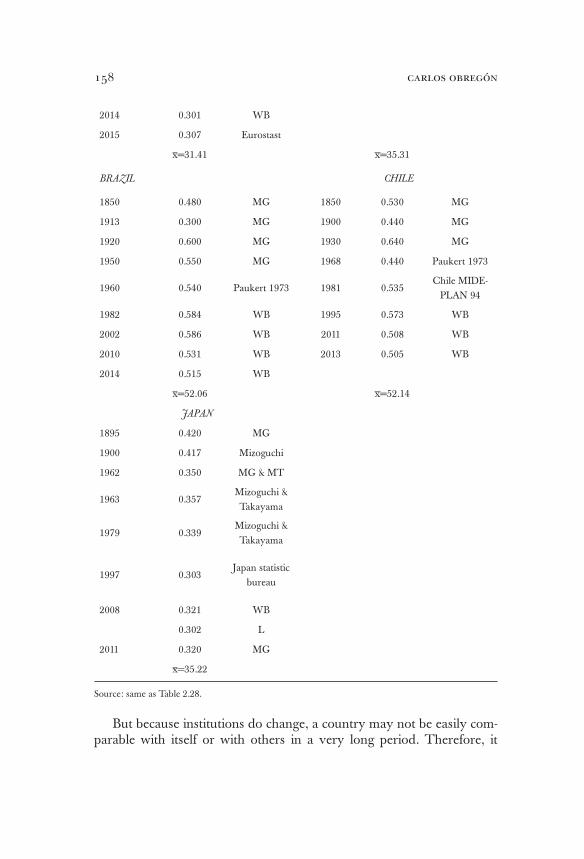
carlos obregón158
2014 0.301 WB
2015 0.307 Eurostast
x=31.41 x=35.31
BRAZIL CHILE
1850 0.480 MG 1850 0.530 MG
1913 0.300 MG 1900 0.440 MG
1920 0.600 MG 1930 0.640 MG
1950 0.550 MG 1968 0.440 Paukert 1973
1960 0.540 Paukert 1973 1981 0.535Chile MIDE-
PLAN 94
1982 0.584 WB 1995 0.573 WB
2002 0.586 WB 2011 0.508 WB
2010 0.531 WB 2013 0.505 WB
2014 0.515 WB
x=52.06 x=52.14
JAPAN
1895 0.420 MG
1900 0.417 Mizoguchi
1962 0.350 MG & MT
1963 0.357Mizoguchi & Takayama
1979 0.339Mizoguchi & Takayama
1997 0.303Japan statistic
bureau
2008 0.321 WB
0.302 L
2011 0.320 MG
x=35.22
Source: same as Table 2.28.
But because institutions do change, a country may not be easily com-parable with itself or with others in a very long period. Therefore, it
nationalism and changes in the income distribution 159
will be useful to also compare them in a shorter period. If we compare countries in modernity —around 1980 to today— we still find profound differences. Japan’s Gini from 1979 to 2011 is flat. The Netherlands from 1983 to 2015 is flat. Italy 1982 to 2015 is almost flat. Germany’s 1973 to today is flat. USA’s 1979 to 2013 is up 0.101. The UK’s 1979 to 2015 is up 0.062. Spain’s 1980 to 2013 is up 0.059. Brazil’s is down 1982 to 2014 0.069, and Chile’s 1981 to 2013 is down 0.03. Thus, four countries’ Ginis are flat or almost flat, three countries are up, and two are down.
Milanovic resumes his Kuznets waves findings in his Table 2.2, in page 88. The countries involved are only six: USA, UK, Spain, Italy, Japan, and Netherlands. And despite using very few countries, he reports huge variances. He reports a level of maximum inequality between 0.51 and 0.61 Gini, but at very different GDP per capita levels that range be-tween 1,500 dollars (1990 PPP’s, Maddison project 2013) and 4,800 dol-lars (300% difference). And a level of minimum inequality that goes from 0.27 to 0.35 Gini again at very different GDP per capita levels that range from 10000 to 19000 dollars (190% difference). The years of downswing of the Kuznets curve go from 50 to 250 years (500% difference). He finds relative commonalities at the expense of huge variances.
Are there really Kuznets waves? The answer is not a straight yes or no. Milanovic has a very interesting proposal that unveils for us the exogenous pressures that push inequality up or down. He does recog-nize institutional factors and the difficulty that one has in forecasting the future. Thus, in some ways one cannot ask for more; but being a scientist, one always does ask for more.
After telling us how difficult forecasting is, Milanovic tries to forecast, and after recognizing the importance of institutional factors, he wants to find strong commonalities instead of exploring institutional differences. There is nothing wrong with that; it is a very scientific procedure. But as very often happens in science, he uncovers the opposite of what he was looking for. His work clearly shows that there is not a general theory that can describe how the income distribution is defined, unless it con-siders historical institutional factors, and the specific exogenous shocks that occur to each country. There are no strong commonalities because there are deep institutional differences. We may theoretically understand what economic or other exogenous shocks, like epidemics or war, may produce in the income distribution, but we cannot forecast when these events will happen nor the magnitude of their impact in the income dis-tribution of a given country —which necessarily depends on it’s specific institutional arrangement.
carlos obregón160
The Kuznets model and the Kuznets waves have a similar problem that Solow’s growth model. Solow’s model can only be rescued (recon-ciled with data) by acknowledging that each country has its own growth path defined by human capital, and its own institutional characteristics. Kuznets’ theory and the Kuznets waves may be rescued by acknowledg-ing that institutional historical factors do give a specific inequality path to each country in a specific historical period. That however, does not solve the problem that some countries are Kuznets’ countries, while others are Kuznets Waves countries, and some are neither.
If we look at Table 2.29 again, we find Kuznets waves in four coun-tries–that is Ginis go up, down, and up again: USA, UK, Germany, and Spain88. We find two Kuznets countries where its Ginis go up and then down: Brazil and Chile89. Moreover, we find three countries which are neither Kuznets countries nor Kuznets waves countries, whose Gini’s mostly just go down as they modernize90.
Milanovic faces the same problem that all the theorists of economic cy-cles have faced: they can describe many of the causes that produce them, but not when they will occur, nor the specific characteristics or magnitude that they will have. Milanovic’s income distribution Kuznets waves theory, like the theorists of economic cycles, lacks predictive power. I have the impres-sion, after listening several lectures from Milanovic, that deep down inside he knows that this is the case. Thus, I do not want to be over critical. His book is an excellent contribution, but there is not a general economic theory that can describe the income distribution, neither as a straight upward line like Piketty has proposed, nor as waves or cycles as Milanovic suggested.
88 USA: up (0.441 -1774 to 0.51 -1860), down (to 0.31 -1979), and up (to 39.5 – 2013); 2) UK: up ( 0.45 – 1688 to 0.575 – 1867), down (to .267 -1979), and up (to .329 – 2013); 3) Germany: up (0.34 – 1882 to 0.396 – 1950), down (to .264 1978), and up (to .307 2015); 4) Spain: up (0.38 – 1850 to 0-54 – 1953), down (to .30 – 1980), and up (to .359 – 2013).
89 Brazil: up (0.48 – 1850 to 0.584 – 1982), and down (to 0.515). Brazil went down before from 0.48 – 1850 to 0.30 – 1913, but this movement, although it is a wave, should not be classified as Kuznets wave because the whole point of Kuznets was that moderniza-tion brings inequality up nor down. Therefore, this movement can be disregarded and the whole movement then looks like Kuznets. 2) Chile: Chile goes first down, and then up, and then down, and then up, and the down again. But because of the same argument used with Brazil, all these movements could be disregarded, and Chile could be seen as a Kuznets country, first up (0.53 - 1850 to 0.573 – 1995), and then down (to 50.5 – 2013).
90 Netherlands, Japan, and Italy. Netherlands goes down (0.55 – 1561 to 0.252 – 1983), and remains almost flat at 0.264 – 2015. Japan goes down (0.42 – 1895 to 0.303 – 1997), and remains almost flat at 0.32 – 2011. Italy goes down (0.51 – 1861 to 0.30 in 1983), and remains almost flat at 0.324 in 2015.

nationalism and changes in the income distribution 161
In their excellent book Lindhert and Williamon list in the first chapter their findings. To conclude this section, I am quoting their last finding:
Inequality movements are driven not by any fundamental law of capitalist develop-
ment but instead by episodic shifts in six basic forces: demography, education policy,
trade competition, finance, and labor saving technological change. These forces
appear to be exogenous with respect to inequality. If they are indeed exogenous and
hard to predict, then four centuries of American inequality can hardly have been
driven by some capitalist law of motion (2016, p 12).
beyond income distribution
We cannot close this chapter without mentioning that economic growth and income distribution are not necessarily the only dimensions that de-fine the well-being of a given society. The excellent work by Nobel Prize winner Amartya Sen has proven that this is the case. On his influence, the United Nations have developed the millennium goals and the HDI —Human Development Index— that consider many more variables of well being and not only income. However, as Bourguignon argues, the problem is that we do not have good historical data to analyze yet and, I would add, not even enough theory.
We will discuss again the HDI in chapter five, but let me advance two conclusions.
1. It is important to look at the HDI when we think about policy actions.
2. The HDI brings additional sources of data, and relevant, but cannot replace the information that income and its distribution provides. The income distribution data, despite its limitations, continues to be very relevant for social analysis.
Before we finish, we would like to briefly mention the consequences of the ICT revolution on poverty.
Poverty and the ICT Revolution
The World Bank 2016 report estimates that in 2013 10.7% of the world population were poor —living below the 1.90 2011 PPP dollars per day—,

carlos obregón162
(see Table 4.5). In millions, they are 767. The ICT meant a huge decrease in the number of poor people. In 1990, the number of poor people was 1,850 millions, and represented 35% of the world population. In 2008, the number was 1,206 millions, and still represented 17.8 % of the world population.
But poverty has not decreased evenly amongst regions. In East Asia and Pacific, mainly due to China, the number of poor people went dra-matically down from 966 millions in 1990 to only 71 millions in 2013; and they went down from representing 60.2% of the population in the re-gion to represent only 3.5%. In Sub Saharan Africa, in the other extreme, the number of poor people increased from 276 millions in 1990 to 389 in 2013, and they still represent 41% of the population in 2013 (down from 54.3% in 1990). In South Asia, the poor still represent 15.1% of the popu-lation (down from 44.6% in 1990). Looking at Table 2.24 we can see that Sub-Saharan Africa also has an income distribution problem, with a Gini of 0.438. And a problem of economic growth, in Table 2.25 we can see that its GDP per capita is only 8.2% the one in high-income countries. South Asia also has a problem of economic growth with an income of only 11.5% the one in high-income countries.
conclusion
As Milanovic has shown, there are external shocks of economic nature and other kind that introduce pressures for more or less inequality in the societies; the ICT revolution is one of such events.
Whenever societies do not have an economic surplus, the income dis-tribution is defined by the land rent subsistence salary ratio, like in the Stationary State of the classical economists.
When an economic surplus is generated, there is margin for inequal-ity to grow. What characterizes capitalism is economic growth due to technological innovations, consequence of the market’s enlargement. Such enlargement is due to two causes: increasing trade due to globaliza-tion forces, and the growing middle class mass consumption of goods produced in the frontier technology. Due to economic growth there is margin for inequality to increase in Capitalism. However, there are two caveats to consider. First, the external technological shocks affect in dis-tinct ways at diverse countries or regions. And second, besides the exter-nal technological shocks there are strong historical institutional arrange-
nationalism and changes in the income distribution 163
ments particular to each country or region that define, together with the shocks, the path taken by the income distribution.
One of the important contributions of Milanovic’s recent book is that it shows together long-term data for diverse countries —that for the USA was possible by the new extraordinary historical analysis made by Lindert and Williamson 2016. Looking at this data one finds very different cases. Some countries follow a Kuznets path, others a Kuznets wave, and some others do not follow either. None of the countries observed is a Piketty’s country —in none of them is there a long run tendency towards a higher Gini. What is clear in this data is that institutional and historical specific forces have had a decisive influence in the final income distribution; and this appears not only in the comparison between diverse countries or regions, but also in comparing the same country in diverse periods.
The history of the twentieth century can not be understood without two key historical factors: the rise of the middle class in the developed economies, and the undeniable fact that this did not happen in the devel-oping economies, nor in the world as a whole. The world’s main prob-lem is not the income distribution in the developed economies, but the income distribution in the world as a whole. The fact that the world is as inequitable as the most underdeveloped and unequal countries should seriously concern us.
However, there is nothing inherently good about a more egalitar-ian income distribution. In fact, during the first century the world was more egalitarian than today, but people in general were much worse off. Capitalism is about economic growth —this is the main feature that dis-tinguishes it. Growth should not, and does not, need to be sacrificed in search of an egalitarian income distribution.
Market dynamics in Capitalism, as Adam Smith taught us, imply eco-nomic freedom, and the selfish search for individual profits will necessar-ily produce some degree of inequality. There are, however, two caveats. The first caveat is that economic growth can happen with very different degrees of inequality —with the economic history both in the West and in Asia this can be shown to be true. Thus, there is ample margin for institu-tional decisions, as to the degree of inequality that is politically desirable.
The second caveat is that extreme inequality does hurt global capital-ist growth. What distinguishes capitalism from previous modes of pro-duction is the enlargement of the market, which is not only due to global trade, but to the growing mass consumption of the middle class. It is the middle class consumption of the growing urban areas that allows for the
carlos obregón164
mass production, which sustains technological development. Previous empires collapsed because enlarging the market through conquest was increasingly expensive as the empire grew in territory. Capitalism instead has its own internal growth dynamics, through the middle class growing consumption. Therefore, several income distribution arrangements are compatible with global capitalist growth, but all of them have to satisfy two conditions: 1) a large middle class, and 2) maintaining incentives for personal profits.
A note of caution, however, is that there is not a straight connection between a country’s middle class and its rate of economic growth, be-cause technology is defined globally by the middle class’ consumption of technological frontier products. Asia developed mainly exporting to the West’s middle class. Attempts to grow the internal market by enlarging a specific country’s middle class have often been big failures, because they end up developing obsolete technology.

[165]
A NEW LOOK AT THE 2008 CRISIS
The 2008 crisis is a good example of how the institutional arrangement, including the old conceptual system, does not respond properly when the technological changes are as abrupt as the ICT revolution has been. In the postwar years of economic stability, the triumphant conceptual system was the neoclassical, on which all of the new generation econo-mists were educated. Keynes’ theoretical contributions that had been so relevant to explain the interwar years of economic instability were no longer studied. Keynes insights were lost in the Monetarist —Keynesian controversy— and by the end of the seventies, Nobel Prize Lucas, among others, had convinced the profession that Keynes was intellectually dead.
The years of the big economic depression were seen as a curiosum–an event of the past, as an outlier in the economic system’s real dynam-ics. The economy system was seen as governed by rational expectations, which meant that all the economic agents had all the available informa-tion, and made proper use of it.
The main reason of the previous disequilibriums was argued to be the irresponsible behavior of prior governments and financial authorities. Therefore, it was enough for them to behave responsible —conserva-tive— and not to make unneeded mistakes for the economy to maintain itself close to the desirable equilibrium. If markets were left alone, they would perform their natural task to maintain the economy in equilib-rium. As we have been arguing, ideas and institutional arrangements go together. Therefore, regulators and official institutions distant them-selves increasingly from the markets, because they wanted to leave the market alone. It was thought that markets, do a better job than the government. The new theoretical thinking developed a new vision of risk, diametrically opposed to Keynes and Knight’s uncertainty, which was thought as more scientific.
In Keynes’ macro thinking, there were two tools to understand how the future’s uncertainty could produce macroeconomic disequilibrium: his theory of the marginal efficiency of capital, and his theory of liquidity preference. Hicks, in his IS-LM model transformed the marginal efficien-cy of capital into the interest rate —investment theory— and therefore

carlos obregón166
eliminated the relationship with the unknown future. And Tobin trans-formed the liquidity preference into his portfolio theory, and replaced the uncertainty related to the unknown future with probabilistic risk —with volatility, which could be measured and known in the present. Institu-tions, therefore, were not needed anymore to bridge into the future. Con-sequently, the economic equilibrium was thought as endogenous, pro-duced by market forces.
In the story we are about to tell about how the 2008 crisis really hap-pened, the main actors are the governments and the financial authorities that did not understand the implications of the ICT revolution, and that, when faced with initial signals of disequilibrium, did not intervene because they thought the markets were going to solve the risky situation by them-selves. The Economic Report of the President argued several years that the markets were going to take care of the subprime real estate crisis, and that they could do it better —more efficiently— than the government. Therefore, there was no need to intervene. The European authorities argued for several years that the subprime crisis was a USA problem not related to them.
How could such prominent economists and regulators have been so wrong? Mainly because of two reasons:
The first one was: That the abrupt changes brought about by the ICT revolution surprised them. Greenspan wrote in his memories that he thought the economic cycles were over, and that the economy could face, for the first time, a very long period of growth. He was facing growth with no inflation due to the Chinese productivity.
That encouraged him to be more aggressive than traditional mon-etary theory would have recommend, and he reduced drastically the Fed’s interest rate in 2001, 2002, and 2003 (see Table 3.1). The Fed’s real interest rate in the period 2001-2005 was for the first time negative, for a five-year period, since 1956 (see Table 3.2).
Why did he do it? He was convinced that due to the low inflation (see Table 3.2, the inflation 1996-2000 was low) the Fed could lower the interest rate without causing inflation, and in this he was right —it was the new world brought about by he ICT revolution. It was an opportu-nity he was decided to take, and in doing so, he was trying to solve two problems: 1) the potential recession of 2001 in which the economy was entering (see Table 3.3); and 2) the crisis in the 80s of the Savings and Loans had left the economy without a good substitute to promote hous-ing for poor people.
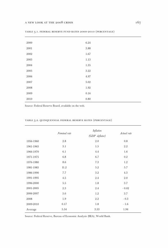
167a new look at the 2008 crisis
table 3.1. federal reserve fund rates 2000-2010 (percentage)
2000 6.24
2001 3.88
2002 1.67
2003 1.13
2004 1.35
2005 3.22
2006 4.97
2007 5.02
2008 1.92
2009 0.16
2010 0.80
Source: Federal Reserve Board, available on the web.
table 3.2. quinquennial federal reserve rates (percentage)
Nominal rateInflation
(GDP deflator)Actual rate
1956-1960 2.8 2.0 0.8
1961-1965 3.1 1.5 2.2
1966-1970 6.1 4.4 1.6
1971-1975 6.8 6.7 0.2
1976-1980 8.6 7.3 1.2
1981-1985 11.2 5.2 5.7
1986-1990 7.7 3.2 4.3
1991-1995 4.5 2.4 2.0
1996-2000 5.5 1.8 3.7
2001-2005 2.3 2.4 - 0.02
2006-2007 5.0 1.2 3.7
2008 1.9 2.2 - 0.3
2009-2010 0.17 1.8 - 1.6
Average 5.54 3.53 1.94
Source: Federal Reserve, Bureau of Economic Analysis (BEA), World Bank.

carlos obregón168
table 3.3. gdp growth per quarter (dollars from 2005)
2001q1 - 1.3
2001q2 2.7
2001q3 - 1.1
2001q4 1.4
2002q1 3.5
2002q2 2.1
2002q3 2.0
2002q4 0.1
2003q1 1.7
2003q2 3.4
2003q3 6.7
2003q4 3.7
2004q1 2.7
2004q2 2.6
2004q3 3.0
2004q4 3.3
Source: Bureau of Economic Statistics (BEA)
The second reason was: The conceptual ideology that markets ad-just by themselves. Greenspan must have known that lowering the interest rate so drastically would produce disequilibriums, but he was not worried because as everybody else, he thought the market could manage them properly.
Surely enough, lowering the interest rate so much did produce disequilibrium; but, the market did not manage it well. Instead, a local disequilibrium in the subprime market became a global banking and economic crisis only second in dimensions to The Great Depression in the 30s.
Greenspan and the regulators underestimated and not fully un-derstood the enormous changes that the ICT revolution had brought about in the financial sector. Due to the ICT revolution, just as manu-facturing had become global, finances did. The banks’ role had dra-matically changed during the ICT revolution; they were no longer local loan providers, but global agencies connecting investors (funds
169a new look at the 2008 crisis
suppliers) with loan seekers (demanding funds). Lowering the interest rate accelerated this process to an extent that the regulators could not foresee. At low interest rates, there were more loan seekers and less suppliers, therefore there was an incentive to make the process more efficient by lowering the intermediation cost. Banks did this by taking the loans out of their books; diminishing the bank’s risk meant they could charge less for the intermediation cost. Their profits increased by managing larger volumes as intermediary agencies, which could be done due to the new technology.
The new securities to be distributed amongst investors were cre-ated bunching distinct classes of loans together. At low interest rates, these new securities became very attractive in yields; and the banks themselves became large holders of these new securities. The sub-prime crisis became generalized for the following reasons:
1. Even though the long-term real estate interest rate is not much influenced by the Fed’s rate —as Greenspan and Bernanke had argued— the adjustable rate is influenced directly. Therefore, more than half of the subprime loans originated with the low-rates were at adjustable rates. And the rapid Fed’s interest rate increased in 2006 and 2007 (see Table 3.1) produced a sharp increase of the monthly payments in these loans (see Table 3.4). And consequently, a rapid increase in default rates in this type of loans (see Table 3.5).
2. These loans have become part of packages —part of the new securities previously described, that were positively rated by the specialized rating agencies. They were well rated for two reasons: a) they include other higher quality loans, and b) the subprime adjustable rates loans previous default rates had not been very high (see Table 3.5).
3. Because of the low interest rates that existed, and the good yields and good rating that these new securities offered, the banks themselves held them. They actually held 75% of the securities back by mortgage loans (MBS securities) not held by subsidized government agencies such as Fannie Mae and Freddie Mack. Therefore, when the subprime crisis started, it involved directly the banks. Thus, a subprime crisis became a banking crisis.
4. These securities were sold globally. Thus, contrary to what the European regulators had been arguing, it was their problem;

carlos obregón170
because their banks had bought the new securities, the crisis became global.
5. The banking crisis pushed up the Libor rate —the interbank rate (see Table 3.6), and as consequence, interest rates in gen-eral went up, and a credit crisis started.
6. The higher interest rates and the low credit generalized the crisis to all the real estate market.
7. Leverage risk taken against the real estate market, even in triple A type of investments, crashed —this explains Lehman’s bankruptcy.
8. Risk was not that manageable after all.
table 3.4. monthly mortgage payment increase
(according to loan year of origination)
Increase percentage
Year of origination 2006 2007
2000 - 16 - 22
2001 24 17
2002 73 63
2003 93 82
2004 76 66
2005 28 19
Source: own calculation based on annual national average one-year adjustable rate loans from http://www.hsh.com (The Trusted Mortgage Resource since 1999) and Federal Reserve data. In this table, the monthly payments are modified based on changes in the Treasury rate of one year.
As we will show, the order of the crisis was as follows: 1. Adjustable rate subprime crisis. 2. Banking crisis —general interest rates go up and credit goes
down. 3. General real estate crisis, because of the higher rates and the
scarce credit.
This order is very important because it clearly shows why the official explanation of the 2008 crisis is incorrect. But before we continue, let us review with some detail the official explanation.

171a new look at the 2008 crisis
TABLE 3.5. MORTGAGE DELINQUENCY RATES (60 DAYS AND MORE)
MORTGAGE LOANS WITH 90 DAYS DELINQUENCY RATE OR IN FORECLOSURE PROCESS.
Fixed rate (FRM)
Adjustable rate (ARM)
Interest only and payment-option loans
2003:1 2004:1 2005:1 2006:1 2007:1
30
25
20
15
10
5
0
35
30
25
20
15
10
5
0
2004 2005 2006 2007 2008
Subprime adjustable rate
(ARM)
Prime adjustable rate (ARM)
Subprime fixed rate
(FRM)
Prime fixed rate (FRM)
2008:Q3
Source: The State of the Nations Housing, Joint Center for Housing Studies of Harvard University 2008.
Mortgage Bankers Association. Economic Report of the President 2009.
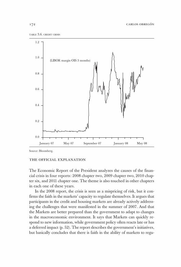
carlos obregón172
the official explanation
The Economic Report of the President analyzes the causes of the finan-cial crisis in four reports: 2008 chapter two, 2009 chapter two, 2010 chap-ter six, and 2011 chapter one. The theme is also touched in other chapters in each one of these years.
In the 2008 report, the crisis is seen as a mispricing of risk, but it con-firms the faith in the markets’ capacity to regulate themselves. It argues that participants in the credit and housing markets are already actively address-ing the challenges that were manifested in the summer of 2007. And that the Markets are better prepared than the government to adapt to changes in the macroeconomic environment. It says that Markets can quickly re-spond to new information, while government policy often reacts late or has a deferred impact (p. 52). The report describes the government’s initiatives, but basically concludes that there is faith in the ability of markets to regu-
Source: Bloomberg.
TABLE 3.6. CREDIT CRISIS
January 07
0.0
0.2
0.4
0.6
0.8
1.0
1.2
May 07 September 07 January 08 May 08
(LIBOR margin OIS 3 months)
173a new look at the 2008 crisis
late themselves. It is also argued that Markets naturally are self-correcting, rewarding good strategies, and punishing bad markets (p.77).
In 2009, the crisis is seen as a serious problem, and a more complete version of what happened is given. The 2009 report explains the crisis in terms similar to those of the Turner’s report to be discussed few para-graphs below. The argument in this 2009 report is as follows:
1. The rapid increase in savings in developing countries produces an excess of ex ante world savings (known as “global savings glut”).
2. Lower interest rates on low risk assets. 3. Investors look for additional performance in higher risk assets
and excess capital inflows are also related to the performance of these assets.
4. As a consequence, a price too low is placed on risk in several markets —houses, commercial real estate, and others; both in the United States and in other countries.
5. Risk with the wrong price is distributed around the world. 6. The inflow of cheap capital is what produces the real estate
price boom. 7. Subprime loan growth and the growth of securities backed by
mortgage loans strengthened the boom. 8. The boom was strengthened by the availability of credit, an
income effect, and very optimistic expectations regarding the future.
9. Both bidders and credit claimers took excessive risk assuming that risky loans could be refinanced or that houses could be sold in case mortgage payments could not be made.
10. The securitization allowed to distribute the risk; and credit standards relaxed, including the subprime loans.
11. The fall in prices in mortgage-backed securities had a significant impact in the financial sector, because a good proportion of these new securities were in banks, investment banks and, other insti-tutions, many of which were financed by short-term loans.
12. Before the crisis, investment banks were leveraged 25 to 1 (i.e. they had investments for 25 times their capital versus 12 to 1 in commercial banking), so that a 4% change in the price of their assets made them lose their capital. And since they were short-term financed, they were very vulnerable to liquidity problems in the market, which made refinancing difficult.
carlos obregón174
13. The bankruptcies of big investment banks, like Bearn Stearns and especially Lehman Brothers, provoked that both investors and banks became conservative, and the credit was severely reduced.
In 2010, chapter 6 analyzes the regulatory deficiencies that led to the crisis. It mentions three regulatory failures:
1. Capital requirements were insufficient, particularly in invest-ment banks.
2. Fragmented regulatory oversight —no one had a global vision. 3. Many of the new institutions were out of regulation such as: mu-
tual funds (mutual funds bought by clients invest in the market directly, and the risks they take are not regulated), and hedge funds (these funds may have very strong leverage i.e. risk many times their clients’ investments and are not regulated).
The consequence is that no regulator understood the speed of conta-gion between the different institutions through the exit of depositors or clients, the sale of assets to hedge positions, and the counterparty risks that became more acute given the credit derivatives boom —because they allowed an institution to transfer the credit risk to another institution without selling the assets.
An example, the famous CDS —credit default swaps that allowed the buyer to secure the risk of not being paid a loan. Mortgage loan securities were secured with CDS. For example, Goldman insured large amounts with AIG. The financial system is designed to perform three functions: produce symmetric information so that depositors or investors understand their risks; transform liquidity creating the opportunity for long-term in-vestments despite short-term deposits; and provide diversification allowing the depositor or saver to participate in a number of investment projects and not just one. Inadequate regulation led to abusive practices, particularly in the subprime markets and non-traditional mortgage lending.
In 2011, the report shows that economic growth from 2001 to 2005 was very unbalanced, according to its historical averages, towards consump-tion expenditures and investment in residences, versus exports and fixed businesses investments. In addition, it indicates that the administration of President Obama should implement a strategy to: 1) reduce the USA’s trade deficit by promoting exports, and 2) increase investment levels.
The version of the Federal Reserve, as expected, was practically the same as that of the President’s Economic Report. Bernanke was in fact the first to coin the term of “global savings glut” (Bernanke, 2005). Also,
175a new look at the 2008 crisis
in various presentations he defended Greenspan’s low interest rate policy arguing that they were necessary to avoid the recession (Bernanke 2010).
In the United Kingdom there are two reports that should be referred to. The first is Turner’s, and the second is the official report presented to the English Parliament in 2009 by the Chancellor. This second report cites Turner’s. The report concludes that: “global regulatory standards, and the global consensus on risk, failed to keep pace with innovation and financial globalization.” It focuses on regulatory reforms, and on strength-ening corporate governance in the national and global financial system.
The Turner report bases its explanation of the crisis on eight pillars, which are:
1. In recent years, large surpluses and deficits have accumulated in the current account balances of various countries. In particu-lar, surpluses in the oil-exporting countries, Japan, China, and other East Asian countries have basically financed the United States’ deficit, but also that of England, Ireland, Spain, and other countries.
2. Current account surpluses are due to an excess of savings, and given the fixed or semi-fixed exchange rates of China and oth-er countries, they have accumulated increasing international reserves in their Central Banks.
3. These reserves are primarily invested in risk-free assets, USA’s Treasury bonds, but also in other countries.
4. This has led to a fall of these risk-free assets real rate to unprec-edented levels, which has stimulated the abundance of credit in general, and mortgage credit in particular.
5. The abundance of mortgage credit generates a real estate boom.
6. Credit standards are degraded, and the cost of such degrada-tion is not understood because with the boom everyone wins.
7. The fall of risk-free assets real rate makes any additional ob-tainable spread very attractive, so that a demand is generated for products that offer that additional spread.
8. This demand was met by financial innovation —by new prod-ucts that securitized mortgage loans, and created the possibility of offering the spread demanded by investors— basically be-cause the new securities did not involve the use of bank capital.
In the European Union, the European Central Bank posted its month-ly Bulletin in January 2011 (entitled “The Financial Crisis and Strength-
carlos obregón176
ening of International Economic Cooperation”) that explains the crisis based on imbalances in current account deficits and surpluses in different countries, coupled with financial sector oversight that lags behind devel-opments. It argues that the dynamics of macro-financial linkages (i.e. the relationship between financial market activity and macroeconomic devel-opments), and macro-prudential linkages (between the prudential regula-tions applicable to financial institutions and their impact in macroeco-nomic developments) were, to a large extent, unexplored. It argues that addressing these shortcomings —the weakness of corrective mechanisms and the lack of understanding of global interrelations— should be a key element of any reform. Finally, it notes that the crisis has made evident the need to improve cooperation and collective action. The report uses elements similar to Turner’s.
The OECD (Organization for Economic Cooperation and Devel-opment) published “Lessons from the Financial Market Turmoil: Chal-lenges ahead for the Financial Industry and Policy Makers”, by Gert Wehinger in 2008. The report consists of four main points:
1. Global liquidity lowers interest rates.2. The origination-distribution model allows to increase the risk a
lot.3. The crisis of the subprime moratorium is triggered. It spreads
to the securities of loan packages, and from there to the balance sheets of the banks and to the cost of interbank funding, then to credit in general.
4. The shares fall, the demand for assets without risk rises, volatility grows very much, and the illiquidity of the market is marked. In the whole process the regulatory environment failed, the responses were disordered and different for each case. Finally, it proposes a series of reforms to the local and global regulatory system. The report overall analysis is very similar to that of Turner.
The IMF (International Monetary Fund) addresses the crisis in many of its reports on financial stability (Global Finance Stability Report). The September 2007 Report discusses that credit standards have deteriorated especially in subprime loans and leveraged loans. April 2008 notes that private sector risk management, transparency, supervision, and regula-tion marched behind financial innovation, and as a consequence, the sys-tem has incurred excessive risk. In October of the same year, it mentions that more losses will come in the United States, that is the epicenter.
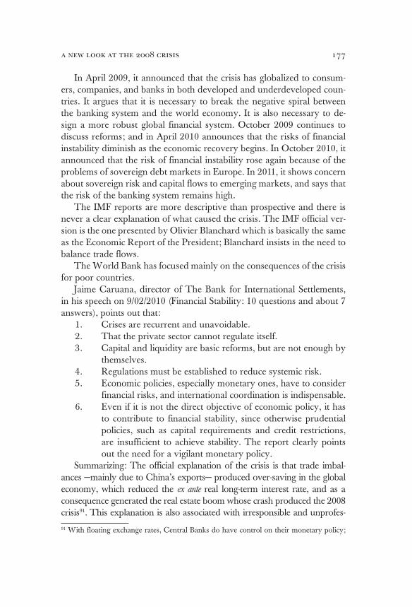
177a new look at the 2008 crisis
In April 2009, it announced that the crisis has globalized to consum-ers, companies, and banks in both developed and underdeveloped coun-tries. It argues that it is necessary to break the negative spiral between the banking system and the world economy. It is also necessary to de-sign a more robust global financial system. October 2009 continues to discuss reforms; and in April 2010 announces that the risks of financial instability diminish as the economic recovery begins. In October 2010, it announced that the risk of financial instability rose again because of the problems of sovereign debt markets in Europe. In 2011, it shows concern about sovereign risk and capital flows to emerging markets, and says that the risk of the banking system remains high.
The IMF reports are more descriptive than prospective and there is never a clear explanation of what caused the crisis. The IMF official ver-sion is the one presented by Olivier Blanchard which is basically the same as the Economic Report of the President; Blanchard insists in the need to balance trade flows.
The World Bank has focused mainly on the consequences of the crisis for poor countries.
Jaime Caruana, director of The Bank for International Settlements, in his speech on 9/02/2010 (Financial Stability: 10 questions and about 7 answers), points out that:
1. Crises are recurrent and unavoidable.2. That the private sector cannot regulate itself. 3. Capital and liquidity are basic reforms, but are not enough by
themselves.4. Regulations must be established to reduce systemic risk. 5. Economic policies, especially monetary ones, have to consider
financial risks, and international coordination is indispensable.6. Even if it is not the direct objective of economic policy, it has
to contribute to financial stability, since otherwise prudential policies, such as capital requirements and credit restrictions, are insufficient to achieve stability. The report clearly points out the need for a vigilant monetary policy.
Summarizing: The official explanation of the crisis is that trade imbal-ances —mainly due to China’s exports— produced over-saving in the global economy, which reduced the ex ante real long-term interest rate, and as a consequence generated the real estate boom whose crash produced the 2008 crisis91. This explanation is also associated with irresponsible and unprofes-
91 With floating exchange rates, Central Banks do have control on their monetary policy;
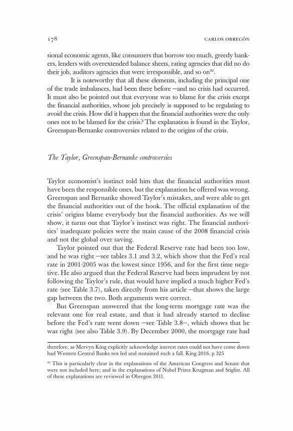
carlos obregón178
sional economic agents, like consumers that borrow too much, greedy bank-ers, lenders with overextended balance sheets, rating agencies that did no do their job, auditors agencies that were irresponsible, and so on92.
It is noteworthy that all these elements, including the principal one of the trade imbalances, had been there before —and no crisis had occurred. It must also be pointed out that everyone was to blame for the crisis except the financial authorities, whose job precisely is supposed to be regulating to avoid the crisis. How did it happen that the financial authorities were the only ones not to be blamed for the crisis? The explanation is found in the Taylor, Greenspan-Bernanke controversies related to the origins of the crisis.
The Taylor, Greenspan-Bernanke controversies
Taylor economist’s instinct told him that the financial authorities must have been the responsible ones, but the explanation he offered was wrong. Greenspan and Bernanke showed Taylor’s mistakes, and were able to get the financial authorities out of the hook. The official explanation of the crisis’ origins blame everybody but the financial authorities. As we will show, it turns out that Taylor’s instinct was right. The financial authori-ties’ inadequate policies were the main cause of the 2008 financial crisis and not the global over saving.
Taylor pointed out that the Federal Reserve rate had been too low, and he was right —see tables 3.1 and 3.2, which show that the Fed’s real rate in 2001-2005 was the lowest since 1956, and for the first time nega-tive. He also argued that the Federal Reserve had been imprudent by not following the Taylor’s rule, that would have implied a much higher Fed’s rate (see Table 3.7), taken directly from his article —that shows the large gap between the two. Both arguments were correct.
But Greenspan answered that the long-term mortgage rate was the relevant one for real estate, and that it had already started to decline before the Fed’s rate went down —see Table 3.8—, which shows that he was right (see also Table 3.9). By December 2000, the mortgage rate had
therefore, as Mervyn King explicitly acknowledge interest rates could not have come down had Western Central Banks not led and sustained such a fall. King 2016, p 325
92 This is particularly clear in the explanations of the American Congress and Senate that were not included here; and in the explanations of Nobel Prizes Krugman and Stiglitz. All of these explanations are reviewed in Obregon 2011.

179a new look at the 2008 crisis
already declined more than one percentage point, while the Fed’s rate had remained high. Greenspan argued that the reason for the decline in the long-term mortgage rate had to be found elsewhere, most likely in ex ante over saving and favorable inflationary expectations.
To show Central Banks responsibility, Taylor pointed out the correla-tion between lower central bank’s rates and higher real estate prices in Europe, r =.19 in Table 3.10 (that comes from the IMF World Economic Outlook), and between Taylor residuals and real state prices in Europe, r = .17 in Table 3.11(from the same source)93.
However, Bernanke shows that they do not hold at the global level, where they are only r =.05 and r = .03 respectively, (see again tables 3.10 and 3.11). Moreover, Bernanke also shows that there is a correlation between current account changes and real estate prices at the global level, r =.24 (see Table 3.12). This settled the score in favor of the Fed. It was off the hook, and trade imbalances, due to over saving mainly in Asia, were to blame.
93 In fact, even a higher correlation could be found, see for example the OECD study for the European Union, which obtains a correlation of .35. Ahrend, Cournede and Price, OECD 2008.
2000 2004 2005 20060
1
2
3
4
5
6
7
2003
Taylor´s rule
Fed´s rate
20022001
Source: The Financial Crisis and the Policy Responses: An Empirical Analysis of What Went Wrong,
Taylor, 2008.
TABLE 3.7 FED´S RATE VERSUS TAYLOR´S RULE
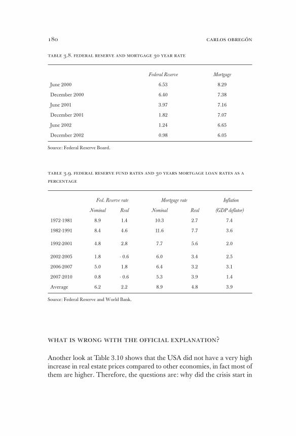
carlos obregón180
table 3.8. federal reserve and mortgage 30 year rate
Federal Reserve Mortgage
June 2000 6.53 8.29
December 2000 6.40 7.38
June 2001 3.97 7.16
December 2001 1.82 7.07
June 2002 1.24 6.65
December 2002 0.98 6.05
Source: Federal Reserve Board.
table 3.9. federal reserve fund rates and 30 years mortgage loan rates as a
percentage
Fed. Reserve rate Mortgage rate Inflation
Nominal Real Nominal Real (GDP deflator)
1972-1981 8.9 1.4 10.3 2.7 7.4
1982-1991 8.4 4.6 11.6 7.7 3.6
1992-2001 4.8 2.8 7.7 5.6 2.0
2002-2005 1.8 - 0.6 6.0 3.4 2.5
2006-2007 5.0 1.8 6.4 3.2 3.1
2007-2010 0.8 - 0.6 5.3 3.9 1.4
Average 6.2 2.2 8.9 4.8 3.9
Source: Federal Reserve and World Bank.
what is wrong with the official explanation?
Another look at Table 3.10 shows that the USA did not have a very high increase in real estate prices compared to other economies, in fact most of them are higher. Therefore, the questions are: why did the crisis start in
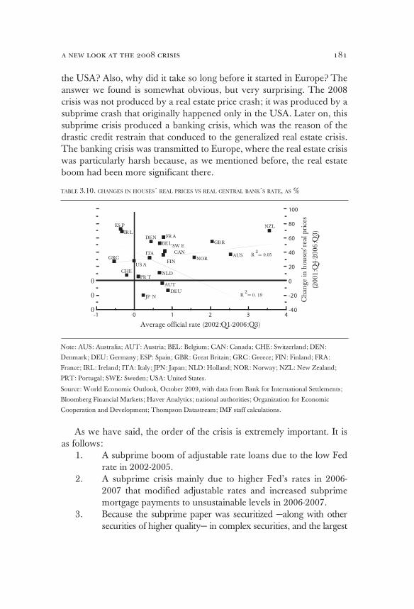
181a new look at the 2008 crisis
the USA? Also, why did it take so long before it started in Europe? The answer we found is somewhat obvious, but very surprising. The 2008 crisis was not produced by a real estate price crash; it was produced by a subprime crash that originally happened only in the USA. Later on, this subprime crisis produced a banking crisis, which was the reason of the drastic credit restrain that conduced to the generalized real estate crisis. The banking crisis was transmitted to Europe, where the real estate crisis was particularly harsh because, as we mentioned before, the real estate boom had been more significant there.
As we have said, the order of the crisis is extremely important. It is as follows:
1. A subprime boom of adjustable rate loans due to the low Fed rate in 2002-2005.
2. A subprime crisis mainly due to higher Fed’s rates in 2006-2007 that modified adjustable rates and increased subprime mortgage payments to unsustainable levels in 2006-2007.
3. Because the subprime paper was securitized —along with other securities of higher quality— in complex securities, and the largest
0
0
0
-1 0 1 2 3 4-40
-20
0
20
40
60
80
100
FIN
FR A
DEU
NLD
ITA
ES P
IR L
R = 0.052
GRC
PR T
AUT
BE L
R = 0. 192
NZL
GB R
AUSNOR
CAN
SW E
DEN
US A
CHE
JP N
Ch
ange
in
hou
ses´
real
pri
ces
(2001:Q
4-2
006:Q
3)
Average official rate (2002:Q1-2006:Q3)
Note: AUS: Australia; AUT: Austria; BEL: Belgium; CAN: Canada; CHE: Switzerland; DEN:
Denmark; DEU: Germany; ESP: Spain; GBR: Great Britain; GRC: Greece; FIN: Finland; FRA:
France; IRL: Ireland; ITA: Italy; JPN: Japan; NLD: Holland; NOR: Norway; NZL: New Zealand;
PRT: Portugal; SWE: Sweden; USA: United States.
Source: World Economic Outlook, October 2009, with data from Bank for International Settlements;
Bloomberg Financial Markets; Haver Analytics; national authorities; Organization for Economic
Cooperation and Development; Thompson Datastream; IMF staff calculations.
TABLE 3.10. CHANGES IN HOUSES´ REAL PRICES VS REAL CENTRAL BANK´S RATE, AS %

carlos obregón182
0
-5 -4 -3 -2 -1 01-40
-20
0
20
40
60
80
100
CAN
NZL
GBR
AUS
US A
SW E
NOR
JP N
R = 0. 172
ES P
IR LFR A
DENBE L
R = 0. 032
GRC
FIN
DEU
AUT
NLDCHE
PR T
ITA
Ch
ange
in
hou
ses´
real
pri
ces
(2001:Q
4-2
006:Q
3)
Average Taylor´s residuals (2002:Q1-2006:Q3)
Note: AUS: Australia; AUT: Austria; BEL: Belgium; CAN: Canada; CHE: Switzerland; DEN:
Denmark; DEU: Germany; ESP: Spain; GBR: Great Britain; GRC: Greece; FIN: Finland; FRA:
France; IRL: Ireland; ITA: Italy; JPN: Japan; NLD: Holland; NOR: Norway; NZL: New Zealand;
PRT: Portugal; SWE: Sweden; USA: United States.
Source: World Economic Outlook, October 2009, with data from Bank for International Settlements;
Bloomberg Financial Markets; Haver Analytics; national authorities; Organization for Economic
Cooperation and Development; Thompson Datastream; IMF staff calculations.
TABLE 3.11. CHANGES IN HOUSES´ REAL PRICES VS TAYLOR´S RESIDUALS, AS %
TABLE 3.12. CHANGES IN HOUSES´ REAL PRICES VS CURRENT ACCOUNT DEFICITS OVER GDP, AS %
Note: AUS: Australia; AUT: Austria; BEL: Belgium; CAN: Canada; CHE: Switzerland; DEN:
Denmark; DEU: Germany; ESP: Spain; GBR: Great Britain; GRC: Greece; FIN: Finland; FRA:
France; IRL: Ireland; ITA: Italy; JPN: Japan; NLD: Holland; NOR: Norway; NZL: New Zealand;
PRT: Portugal; SWE: Sweden; USA: United States.
Source: World Economic Outlook, October 2009, with data from Bank for International Settlements;
Bloomberg Financial Markets; Haver Analytics; national authorities; Organization for Economic
Cooperation and Development; Thompson Datastream; IMF staff calculations.
Chan
ge in h
ouse
s´ re
al p
rice
s
(2001:Q
4–2006:Q
3)
Average percentual quarterly change in current account
over GDP (2002:Q1–2006:Q3)ttt
-0.4 -0.2 0 0.2 0.4 0.6-40
-20
0
20
40
60
80
100
R = 0.242
NLDCHE
DEUJP N
SWECANAUS
ESP NZLFRA GBR
IRL
DEN
NORFIN ITA
USA
AUT
GRC
PRT
BEL

183a new look at the 2008 crisis
share (75%) of MBS in the private sector, excluding agencies subsidies by the government, was held by the banks; we enter a banking crisis that starts officially in august 10, 2007.
4. This meant higher interbank and lending rates and less credit available.
5. The higher rates and lower credit then produced a generalized real estate and a stock market crash.
6. The worsening of consumers’ and institutions’ balance sheets explains the extent, size, and duration of the crisis.
In what follows, we will document our explanation. Yet, before we do it, it is necessary to emphasize the importance of defining: what really happened? If we assume for a moment that the official explanation is cor-rect, that means that we have to acknowledge that the markets had pro-duced unsustainable trade imbalances which have to be rebalanced —Ol-ivier Blanchard’s argument in the Sept 2011 WEO-IMF report. But since it is incorrect, we do not need to do so. Balanced trade means less trade, closing the door for underdeveloped economies to develop, and lowering the living standard in the developed economies94. Since unbalanced trade did not produce the crisis, it means that we should reconsider the need to balance it —particularly in the USA case, whose trade deficit has been an engine for the growth of the global economy and a mechanism to elevate the standard of living of the USA citizens; a win win situation. These ideas will be further explored in chapter four.
Did real estate crash before the banking crisis?
The critical issue is whether the banking crisis was a consequence of a real estate crash, like the official view states, or whether it was the other way around, as we argue. The question is empirically very simple: Did real estate prices crash before august 10, 2007 or not? The answer, how-ever, is not as straightforward. It partially depends in which real estate
94 For the USA to balance its trade account without reducing global trade; China, Japan and other countries would have to consume more but they are not ready for this. Their economies are geared towards exports. Take the case of China, its population in general is too poor to consume the middle class frontier products produced in the USA. If, for example, China does not increase its imports, the only way out to balance trade accounts is for the USA to import less, which means reducing global trade, with all the implications previously mentioned.
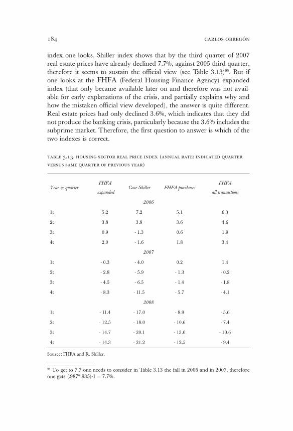
carlos obregón184
index one looks. Shiller index shows that by the third quarter of 2007 real estate prices have already declined 7.7%, against 2005 third quarter, therefore it seems to sustain the official view (see Table 3.13)95. But if one looks at the FHFA (Federal Housing Finance Agency) expanded index (that only became available later on and therefore was not avail-able for early explanations of the crisis, and partially explains why and how the mistaken official view developed), the answer is quite different. Real estate prices had only declined 3.6%, which indicates that they did not produce the banking crisis, particularly because the 3.6% includes the subprime market. Therefore, the first question to answer is which of the two indexes is correct.
table 3.13. housing sector real price index (annual rate: indicated quarter
versus same quarter of previous year)
Year & quarterFHFA
expandedCase-Shiller FHFA purchases
FHFA
all transactions
2006
1t 5.2 7.2 5.1 6.3
2t 3.8 3.8 3.6 4.6
3t 0.9 - 1.3 0.6 1.9
4t 2.0 - 1.6 1.8 3.4
2007
1t - 0.3 - 4.0 0.2 1.4
2t - 2.8 - 5.9 - 1.3 - 0.2
3t - 4.5 - 6.5 - 1.4 - 1.8
4t - 8.3 - 11.5 - 5.7 - 4.1
2008
1t - 11.4 - 17.0 - 8.9 - 5.6
2t - 12.5 - 18.0 - 10.6 - 7.4
3t - 14.7 - 20.1 - 13.0 - 10.6
4t - 14.3 - 21.2 - 12.5 - 9.4
Source: FHFA and R. Shiller.
95 To get to 7.7 one needs to consider in Table 3.13 the fall in 2006 and in 2007, therefore one gets (.987*.935)-1 = 7.7%.
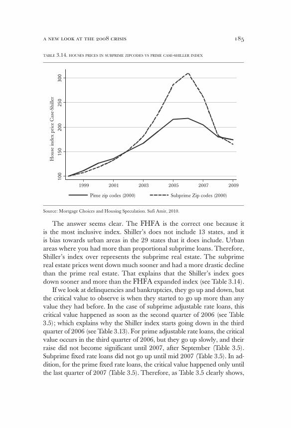
185a new look at the 2008 crisis
The answer seems clear. The FHFA is the correct one because it is the most inclusive index. Shiller’s does not include 13 states, and it is bias towards urban areas in the 29 states that it does include. Urban areas where you had more than proportional subprime loans. Therefore, Shiller’s index over represents the subprime real estate. The subprime real estate prices went down much sooner and had a more drastic decline than the prime real estate. That explains that the Shiller’s index goes down sooner and more than the FHFA expanded index (see Table 3.14).
If we look at delinquencies and bankruptcies, they go up and down, but the critical value to observe is when they started to go up more than any value they had before. In the case of subprime adjustable rate loans, this critical value happened as soon as the second quarter of 2006 (see Table 3.5); which explains why the Shiller index starts going down in the third quarter of 2006 (see Table 3.13). For prime adjustable rate loans, the critical value occurs in the third quarter of 2006, but they go up slowly, and their raise did not become significant until 2007, after September (Table 3.5). Subprime fixed rate loans did not go up until mid 2007 (Table 3.5). In ad-dition, for the prime fixed rate loans, the critical value happened only until the last quarter of 2007 (Table 3.5). Therefore, as Table 3.5 clearly shows,
TABLE 3.14. HOUSES PRICES IN SUBPRIME ZIPCODES VS PRIME CASE-SHILLER INDEX
300
250
200
150
100
1999 2001 2003 2005 2007 2009
Subprime Zip codes (2000)Pime zip codes (2000)
Hou
se in
dex
pri
ce C
ase-
Sh
ille
r
Source: Mortgage Choices and Housing Speculation. Sufi Amir, 2010.
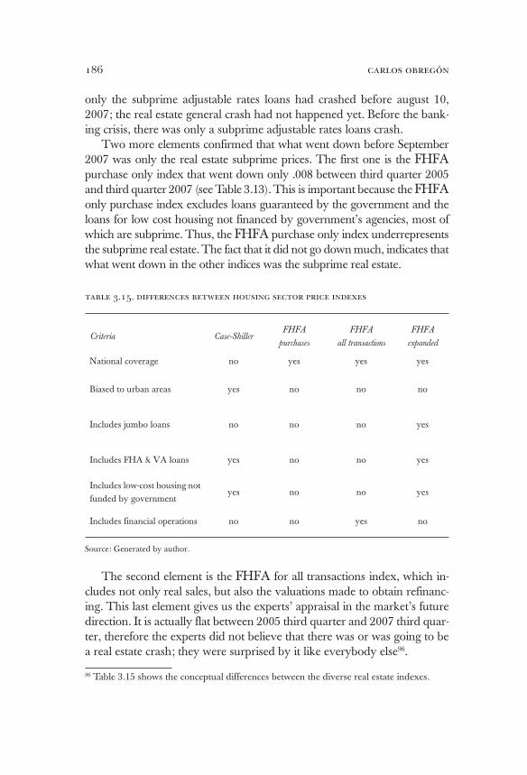
carlos obregón186
only the subprime adjustable rates loans had crashed before august 10, 2007; the real estate general crash had not happened yet. Before the bank-ing crisis, there was only a subprime adjustable rates loans crash.
Two more elements confirmed that what went down before September 2007 was only the real estate subprime prices. The first one is the FHFA purchase only index that went down only .008 between third quarter 2005 and third quarter 2007 (see Table 3.13). This is important because the FHFA only purchase index excludes loans guaranteed by the government and the loans for low cost housing not financed by government’s agencies, most of which are subprime. Thus, the FHFA purchase only index underrepresents the subprime real estate. The fact that it did not go down much, indicates that what went down in the other indices was the subprime real estate.
table 3.15. differences between housing sector price indexes
Criteria Case-ShillerFHFA
purchases
FHFA
all transactions
FHFA
expanded
National coverage no yes yes yes
Biased to urban areas yes no no no
Includes jumbo loans no no no yes
Includes FHA & VA loans yes no no yes
Includes low-cost housing not funded by government
yes no no yes
Includes financial operations no no yes no
Source: Generated by author.
The second element is the FHFA for all transactions index, which in-cludes not only real sales, but also the valuations made to obtain refinanc-ing. This last element gives us the experts’ appraisal in the market’s future direction. It is actually flat between 2005 third quarter and 2007 third quar-ter, therefore the experts did not believe that there was or was going to be a real estate crash; they were surprised by it like everybody else96.
96 Table 3.15 shows the conceptual differences between the diverse real estate indexes.
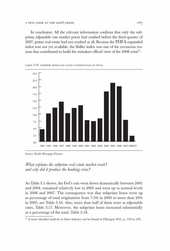
187a new look at the 2008 crisis
In conclusion: All the relevant information confirms that only the sub-prime adjustable rate market prices had crashed before the third quarter of 2007; prime real estate had not crashed at all. Because the FHFA expanded index was not yet available, the Shiller index was one of the erroneous rea-sons that contributed to build the mistaken official view of the 2008 crisis97.
What explains the subprime real estate market crash? and why did it produce the banking crisis?
As Table 3.1 shows, the Fed’s rate went down dramatically between 2001 and 2004, remained relatively low in 2005 and went up to normal levels in 2006 and 2007. The consequence was that subprime loans went up as percentage of total originations from 7.5% in 2003 to more than 20% in 2005, see Table 3.16. Also, more than half of them were at adjustable rates, Table 3.17. Moreover, the subprime loans increased substantially as a percentage of the total, Table 3.18.97 A more detailed analysis in these indexes can be found in Obregon 2011, p. 139 to 150.
TABLE 3.16. SUBPRIME MORTGAGE LOANS AS PERCENTAGE OF TOTAL
Source: Inside Mortgage Finance.
1994 1995 1996 1997 1998 1999 2000 2001 2002 2003 2004 2005 2006 2007
0.0
2.5
5.0
7.5
10.0
12.5
15.0
17.5
20.0
22.5
25.0
2008 Q1
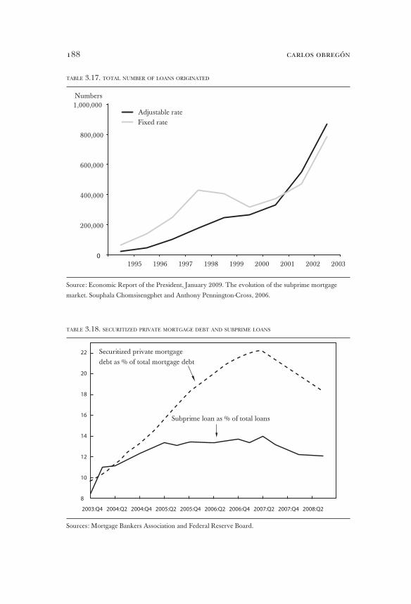
carlos obregón188
TABLE 3.17. TOTAL NUMBER OF LOANS ORIGINATED
0
200,000
400,000
600,000
800,000
1,000,000
Numbers
Adjustable rate
Fixed rate
1995 1996 1997 1998 1999 2000 2001 2002 2003
Source: Economic Report of the President, January 2009. The evolution of the subprime mortgage
market. Souphala Chomsisengphet and Anthony Pennington-Cross, 2006.
TABLE 3.18. SECURITIZED PRIVATE MORTGAGE DEBT AND SUBPRIME LOANS
22
20
18
16
14
12
10
8
2003:Q4 2004:Q42004:Q2 2005:Q2 2006:Q2 2006:Q4 2007:Q2 2008:Q22007:Q42005:Q4
Securitized private mortgage
debt as % of total mortgage debt
Subprime loan as % of total loans
Sources: Mortgage Bankers Association and Federal Reserve Board.
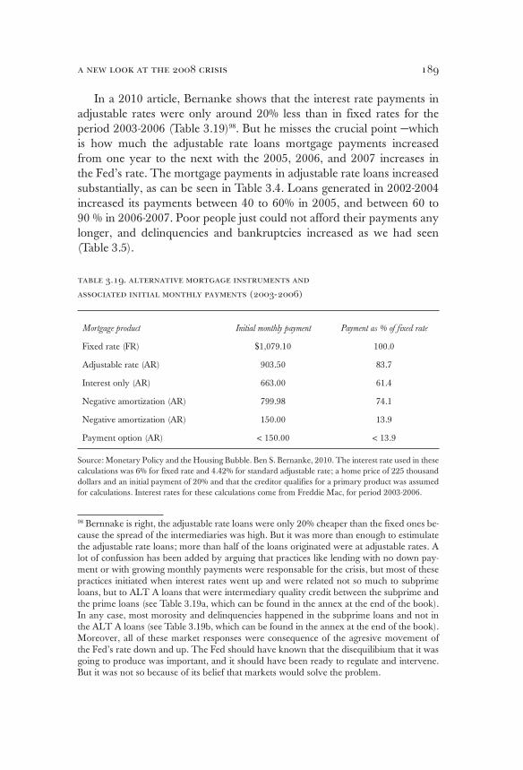
189a new look at the 2008 crisis
In a 2010 article, Bernanke shows that the interest rate payments in adjustable rates were only around 20% less than in fixed rates for the period 2003-2006 (Table 3.19)98. But he misses the crucial point —which is how much the adjustable rate loans mortgage payments increased from one year to the next with the 2005, 2006, and 2007 increases in the Fed’s rate. The mortgage payments in adjustable rate loans increased substantially, as can be seen in Table 3.4. Loans generated in 2002-2004 increased its payments between 40 to 60% in 2005, and between 60 to 90 % in 2006-2007. Poor people just could not afford their payments any longer, and delinquencies and bankruptcies increased as we had seen (Table 3.5).
table 3.19. alternative mortgage instruments and
associated initial monthly payments (2003-2006)
Mortgage product Initial monthly payment Payment as % of fixed rate
Fixed rate (FR) $1,079.10 100.0
Adjustable rate (AR) 903.50 83.7
Interest only (AR) 663.00 61.4
Negative amortization (AR) 799.98 74.1
Negative amortization (AR) 150.00 13.9
Payment option (AR) < 150.00 < 13.9
Source: Monetary Policy and the Housing Bubble. Ben S. Bernanke, 2010. The interest rate used in these calculations was 6% for fixed rate and 4.42% for standard adjustable rate; a home price of 225 thousand dollars and an initial payment of 20% and that the creditor qualifies for a primary product was assumed for calculations. Interest rates for these calculations come from Freddie Mac, for period 2003-2006.
98 Bernnake is right, the adjustable rate loans were only 20% cheaper than the fixed ones be-cause the spread of the intermediaries was high. But it was more than enough to estimulate the adjustable rate loans; more than half of the loans originated were at adjustable rates. A lot of confussion has been added by arguing that practices like lending with no down pay-ment or with growing monthly payments were responsable for the crisis, but most of these practices initiated when interest rates went up and were related not so much to subprime loans, but to ALT A loans that were intermediary quality credit between the subprime and the prime loans (see Table 3.19a, which can be found in the annex at the end of the book). In any case, most morosity and delinquencies happened in the subprime loans and not in the ALT A loans (see Table 3.19b, which can be found in the annex at the end of the book). Moreover, all of these market responses were consequence of the agresive movement of the Fed’s rate down and up. The Fed should have known that the disequilibium that it was going to produce was important, and it should have been ready to regulate and intervene. But it was not so because of its belief that markets would solve the problem.
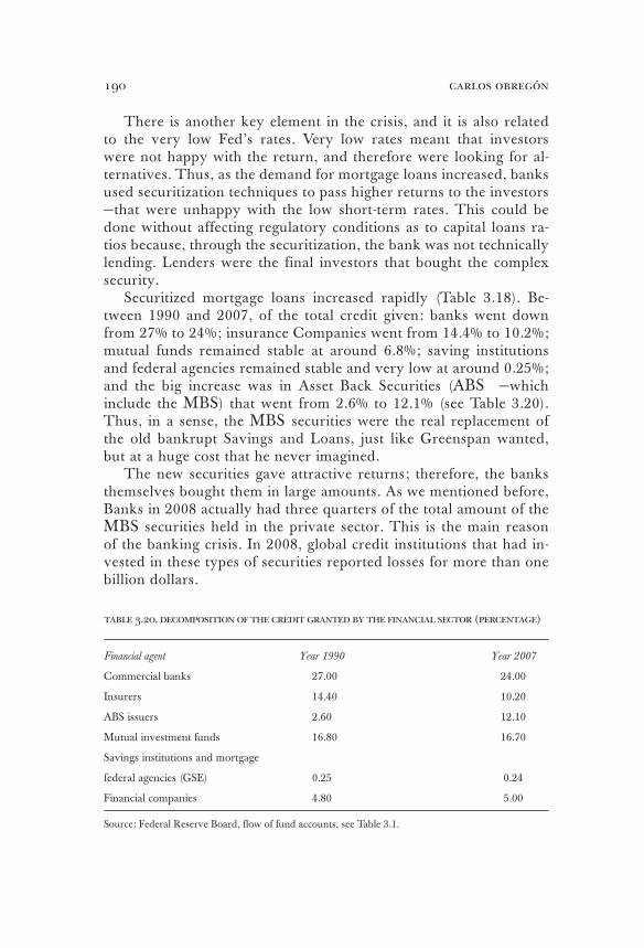
carlos obregón190
There is another key element in the crisis, and it is also related to the very low Fed’s rates. Very low rates meant that investors were not happy with the return, and therefore were looking for al-ternatives. Thus, as the demand for mortgage loans increased, banks used securitization techniques to pass higher returns to the investors —that were unhappy with the low short-term rates. This could be done without affecting regulatory conditions as to capital loans ra-tios because, through the securitization, the bank was not technically lending. Lenders were the final investors that bought the complex security.
Securitized mortgage loans increased rapidly (Table 3.18). Be-tween 1990 and 2007, of the total credit given: banks went down from 27% to 24%; insurance Companies went from 14.4% to 10.2%; mutual funds remained stable at around 6.8%; saving institutions and federal agencies remained stable and very low at around 0.25%; and the big increase was in Asset Back Securities (ABS —which include the MBS) that went from 2.6% to 12.1% (see Table 3.20). Thus, in a sense, the MBS securities were the real replacement of the old bankrupt Savings and Loans, just like Greenspan wanted, but at a huge cost that he never imagined.
The new securities gave attractive returns; therefore, the banks themselves bought them in large amounts. As we mentioned before, Banks in 2008 actually had three quarters of the total amount of the MBS securities held in the private sector. This is the main reason of the banking crisis. In 2008, global credit institutions that had in-vested in these types of securities reported losses for more than one billion dollars.
table 3.20. decomposition of the credit granted by the financial sector (percentage)
Financial agent Year 1990 Year 2007
Commercial banks 27.00 24.00
Insurers 14.40 10.20
ABS issuers 2.60 12.10
Mutual investment funds 16.80 16.70
Savings institutions and mortgage
federal agencies (GSE) 0.25 0.24
Financial companies 4.80 5.00
Source: Federal Reserve Board, flow of fund accounts, see Table 3.1.

191a new look at the 2008 crisis
the mismanagement of the crisis
For three years, the Fed and the economic report of the president argued that the markets were going to take care of the subprime crisis, and the Eu-ropean regulators insisted that it was a USA problem that did not concern them. They all were wrong. Despite the fact that the subprime loan market was not that large, the securities that represented them were already part of complex securities held in large amounts by the banks all over the world, and subprime bankruptcies made it impossible to value the complex securi-ties. Therefore, banks became concerned with one another’s good credit. The interbank lending rate —Libor— rose dramatically in August 10, 2007 signaling the beginning of the banking crisis (again Table 3.6).
The banking crisis was mismanaged by the financial authorities. It was required to sustain the market price of the subprime mortgag-es by buying a portion of them at a discount. With a given reason-able price for the subprime loans, the complex securities would have been valued properly, and banks would have known how to evalu-
Source: Inside Mortgage Finance.
TABLE 3.21. TOTAL SUBPRIME LOANS IN THE SYSTEM
0
200
400
600
800
1000
1200
1400
1995 1996 1997 1998 1999 2000 2001 2002 2003 2004 2005 2006 2007 2008 1Q
290 283 319 344382
416479
574
699
940895
973
1,200 1,240Total amount of subprime mortgage loans
US $ Billion dollars
carlos obregón192
ate each other and we would not have had a banking crisis. Since the total value of the subprime mortgages in 2006 was only 1240 billion dollars (see Table 3.21), given the delinquencies and bankruptcies rates of 6% and 3%, a rescue program for 200 billion dollars would have been more than enough. Let us assume a 100 billion dollars cost of such a program (which is in the upside). Banks could have absorbed half of this amount, let us say repaying the government in a ten-year period. There were many other options, and all of them, if applied early enough, would have been extremely cheap compared to the costs incurred later on. Instead, the authorities waited for the market to solve the problem. They did not realize the cost of waiting because they did not understand the complex global links that the financial system had brought about due to the ICT revolution.
A large part of the financial system was based on instruments pricing assets volatility, like derivatives and others. Waiting meant allowing the volatility to increase out of forecastable ranges; it was very dangerous. Moreover, USA banks total capital was 700 billion dollars and their profits only 113 in 2006, therefore, the amounts involved were too high for the banks to manage it by themselves (see Table 3.22).
Before August 10, 2007, the authorities did not intervene. After this day, there were diverse interventions to provide the market with extra liquidity. But, the bank’s problem was solvency, not liquidity. As long as they had the subprime loans embedded in complex secu-rities in their balance sheets, more liquidity was not going to help.
The banking crisis continued surprising the authorities, which responded chaotically without a well-designed program. Many cru-cial financial institutions entered serious problems or went bankrupt. On March 14, Bear Stearns; on July 11, Indy Mac; September 8, Fannie Mae and Freddie Mac; September 15, Lehman Brothers; Sep-tember 15, Merril Lynch and Co.; September 16, AIG; September 25, Washington Mutual Inc.; September 29, Wachovia. Bear Stearns was rescued, AIG was bail out, Lehman Brothers was not rescued. AIG bailed out prevented Goldman Sachs from facing bankruptcy. Goldman had huge amounts of CDS —credit default swaps— from AIG, which were paid, controversially, at full price.
The erratic public policy made the market very nervous and the interbank rate high rocket (see Table 3.23). In September 19, the TARP program (Troubled Asset Relief Program) announced it was

193a new look at the 2008 crisis
buying toxic securities from the banks —finally a step in the right direction, but was soon abandoned and transformed only in provid-ing more capital to the banks (see Table 3.24). By then the solvency problem had become very acute; the balance of the banks was in disarray. The decision to not rescue Lehman was a systemic mis-take. Additional capital was not going to solve the problem —and it did not. Finally, the Federal Reserve had to print large amounts of money, and enter the market to buy toxic securities for more than two billion dollars because the treasury did not do its job.
table 3.22. assets, capital and earnings of main north american banks (bil-
lions of dollars, end of 2006)
2006
EarningsAssets Capital
2007
Earnings
2008
Earnings
Citigroup 22 1 884 120 4 - 10
Bank of America 21 1 460 135 15 6
JP Morgan Chase 14 1352 116 15 5
Morgan Stanley 7 1 121 35 3 4
Merril Lynch 7 841 39 - 8 - 12
Fannie Mae 4 835 42 - 2 - 33
Goldman Sachs 10 835 36 12 4
Freddie Mac 2 813 28 - 3 - 26
Wachovia 8 707 70 6 - 33
Lehman 4 501 19 4 - 6
Wells Fargo 8 482 46 8 5
Bear Stearns 2 350 12 0 #NA
Wa Mu 4 346 27 0 #NA
Source: FactSet, COMPUSTAT.
It is important to realize that the 2008 crisis was not produced by global trade imbalances and over saving, as the official version argues. It was just a typical credit crisis. A theoretical framework to understand what really happened is provided by Minsky (whose model was used by Kindleberger in his famous book Manias, Panics, and Crisis) and Keynes; both will be re-viewed for the theoretical inclined reader at the end of this chapter.

carlos obregón194
January 07
0.0
0.5
2.5
1.5
3.0
1.0
2.0
July 08January 08 April 08 October 09April 07 October 07
(Margin LIBOR-OIS)
3.5
4.0
TABLE 3.23. THE CREDIT CRISIS CONTINUES
Source: Bloomberg.
July 07
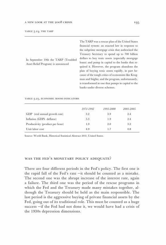
195a new look at the 2008 crisis
table 3.24. the tarp
In September 19th the TARP (Troubled Asset Relief Program) is announced
The TARP was a rescue plan of the United States financial system: an enacted law in response to the subprime mortgage crisis that authorized the Treasury Secretary to spend up to 700 billion dollars to buy toxic assets (especially mortgage loans) and pump in capital to the banks that re-quired it. However, the program abandons the plan of buying toxic assets rapidly, in part be-cause of the tough critics of economists like Krug-man and Stiglitz, and the program, unfortunately, is transformed in one that pumps in capital to the banks under diverse schemes.
table 3.25. economic boom indicators
1971-1992 1993-2000 2001-2005
GDP (real annual growth rate) 3.2 3.9 2.4
Inflation (GDP´s deflator) 5.3 1.9 2.4
Productivity (product per hour) 1.9 2.0 3.2
Unit labor cost 4.9 1.7 0.8
Source: World Bank, Historical Statistical Abstract 2011, United States.
was the fed’s monetary policy adequate?
There are four different periods in the Fed’s policy. The first one is the rapid fall of the Fed’s rate —it should be counted as a mistake. The second one was the abrupt increase of the interest rate, again a failure. The third one was the period of the rescue programs in which the Fed and the Treasury made many mistakes together, al-though the Treasury should be held as the main responsible. The last period is the aggressive buying of private financial assets by the Fed, going out of its traditional role. This must be counted as a huge success —if the Fed had not done it, we would have had a crisis of the 1930s depression dimensions.

carlos obregón196
Greenspan was right: a new world was coming due to the ICT revolution, and there was no reason to be afraid of inflation. Table 3.25 shows that because of the the ICT revolution from 1993 to 2000 the GDP growth went up, inflation went down, productivity went up, and the labor unitary cost went down. Therefore, Greenspan was correct. There was no need to miss the potential future growth that the econo-my could have. He understood very cleverly some of the the ICT revo-lution’s dimensions, but he was too aggressive. There was no need of such aggressive moves in the Fed’s rate. A correction is always welcome in the markets, and the medium upward trend would not have stopped, had the Fed not decreased so aggressively the interest rate. In fact, the short-term correction needed, happened anyway in the stock market (see Table 3.26)99. Why? Precisely because of the same argument that Greenspan used later on: the Fed’s rate cannot change the fundamental trend of the long interest rate, which obeys more structural factors.
Table 3.28 presents the fiscal policy that Greenspan faced. As it can be seen, from 2001 to 2005, government’s deficit was only 1.9% of the GDP, small compared for example to what Volcker faced. From 1981-1988 it was 4.2, and from 1989-1992 was 4.0. Greenspan did face a larger current account deficit of 4.8%, but was coming from the private sector due to the ICT revolution–and was actually one of the reasons for the low inflation. Thus, from the fiscal side, he did not have to worry too much. But, there was no need either to bring the interest rate down so much.
99 In fact, the real estate market and the stock market follow their own tendencies, guided by the long-term interest rate and their own value characteristics, which were actually in opposite directions: The Stock Market went down and the Real Estate Market went up. Why? Because the Stock market had risen a lot in the 90s and was expensive, while the Real estate market was not. Between 1993 and 2000, the stock market rised 12% annually in real terms because expected future profits got up a lot (Table 3.26), while the real estate market only went up 2.1% annually in real terms. The P/E was high in the period 1993-2000. As can be seen in Table 3.26, it was 26.6, therefore stocks became expensive, while the rent price ratio was in the same period around 4.7 (see Table 3.27), hence real estate was still relative cheap. How do you compare both numbers? You multiply the rent price ratio by the real rate of annual return for real estate, and you end up with 6.8%. To this number you have to deduct the expenses incur to be able to rent, you probably end up with a number slightly lower than 6%, less than half the annual return in the Stock Market in 1993-2000. But 26.6 in the stock market means only 4.4 expected return, too low for historical standards. The average historical return since 1881 was 6.1% with a P/E 10 (calculated 10 years backwards) of 16.42. Therefore, the Stock market had become expensive; while the 4.7 in the rent price ratio was normal for historical standards. The stock market always looks forward and the outlook was for good profits, but the price was already too high. With the stock market adjusting, the consumer wealth high, a reasonable rent price ratio, and inflationary expectations low,bringing down the long-term interest rate all theconditions were there for the beginning of the real estate boom in 2000. But any way, real estate prices in the USA went up significantly less than in Europe (see Table 3.11).

197a new look at the 2008 crisis
table 3.26. usa stock market
(annual yield %, p/e and p/e10 in the last year of the period)
P/E P/E10 Nominal Yield Real yield
1971-1976 10.6 11.6 2.5 -3.8
1977-1980 9.0 9.4 6.3 -3.7
1981-1988 11.6 14.7 9.5 5.0
1989-1992 22.8 20.5 12.0 7.6
1993-2000 26.6 37.3 15.0 12.1
2001-2005 18.0 26.4 -1.1 -3.5
2006-2007 22.0 26.0 8.3 4.8
2008-2010 16.0 22.4 -5.7 -7.0
2011 (August) 13.7 20.3 -6.7 -11.2
Source: S & P500. Actual performance is deflated by the Consumer Price Index (CPI). Real yield is
calculated without dividends.
Table 3.29 compares Greenspan monetary policy with other periods. As it can be seen, there was no precedent for his aggressiveness. There was nothing in monetary theory that suggested that Greenspan could really in-fluence the long-term growth path of the economy, which is given by struc-tural factors —as Friedman and Schwartz (1963) had concluded many years ago. In the long-term, money only influences prices; in the short-term, the economic cycle can be influenced by monetary policy if the bank is cred-ible —that means if the market believes that a future low inflation is cred-ible. Hence, a Fed’s intervention to influence the short-term economic cycle may be justifiable. But, notice in Table 3.3 that by the first quarter of 2002 the economy was already growing normally, thus not even the economic short-term cycle justification was there anymore. Greenspan maintains the rates low too long because of the housing for the poor, and his belief that there were no limits anymore in the economy’s growth potential. Given the ICT revolution, the Fed thought it could be much more aggressive than usual. And even though he does not recognize it, he did not like the adjust-ment that the stock market was having. For him the future was brighter. In many ways, given the ICT revolution, he was right. Nevertheless, it is not the central banker’s job to join the party, but to close the door at certain hour and to maintain the party under control. Greenspan, in our opinion, got too involved with the market to be able to maintain his role as referee.
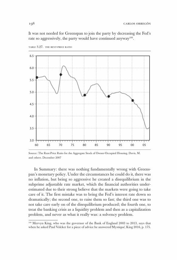
carlos obregón198
It was not needed for Greenspan to join the party by decreasing the Fed’s rate so aggressively, the party would have continued anyway100.
In Summary: there was nothing fundamentally wrong with Greens-pan’s monetary policy. Under the circumstances he could do it, there was no inflation, but being so aggressive he created a disequilibrium in the subprime adjustable rate market, which the financial authorities under-estimated due to their strong believe that the markets were going to take care of it. The first mistake was to bring the Fed’s interest rate down so dramatically; the second one, to raise them so fast; the third one was to not take care early on of the disequilibrium produced; the fourth one, to treat the banking crisis as a liquidity problem and then as a capitalization problem, and never as what it really was: a solvency problem.
100 Mervyn King, who was the governor of the Bank of England 2003 to 2013, says that when he asked Paul Volcker for a piece of advice he answered Mystique¨, King 2016, p. 175.
Source: The Rent-Price Ratio for the Aggregate Stock of Owner-Occupied Housing. Davis, M.
and others. December 2007
TABLE 3.27. THE RENT-PRICE RATIO
3.0
3.5
4.0
4.5
5.0
5.5
6.0
6.5
60 65 70 75 80 85 90 95 00 05
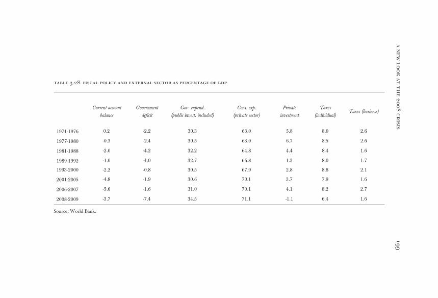
19
9a
new
lo
ok
at
th
e 2
00
8 c
ris
is
table 3.28. fiscal policy and external sector as percentage of gdp
Current account
balance
Government
deficit
Gov. expend.
(public invest. included)
Cons. exp.
(private sector)
Private
investment
Taxes
(individual)Taxes (business)
1971-1976 0.2 -2.2 30.3 63.0 5.8 8.0 2.6
1977-1980 -0.3 -2.4 30.5 63.0 6.7 8.5 2.6
1981-1988 -2.0 -4.2 32.2 64.8 4.4 8.4 1.6
1989-1992 -1.0 -4.0 32.7 66.8 1.3 8.0 1.7
1993-2000 -2.2 -0.8 30.5 67.9 2.8 8.8 2.1
2001-2005 -4.8 -1.9 30.6 70.1 3.7 7.9 1.6
2006-2007 -5.6 -1.6 31.0 70.1 4.1 8.2 2.7
2008-2009 -3.7 -7.4 34.5 71.1 -1.1 6.4 1.6
Source: World Bank.
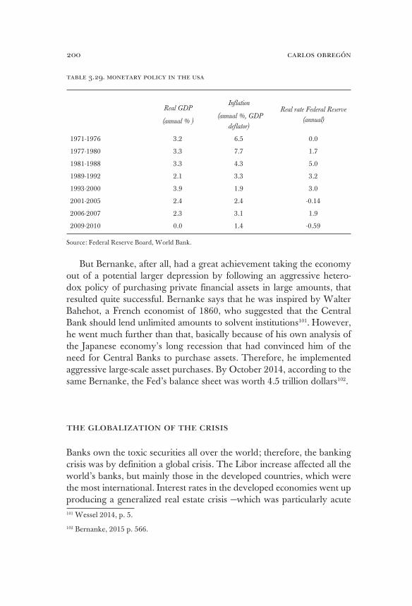
carlos obregón200
table 3.29. monetary policy in the usa
Real GDP
(annual % )
Inflation
(annual %, GDP
deflator)
Real rate Federal Reserve
(annual)
1971-1976 3.2 6.5 0.0
1977-1980 3.3 7.7 1.7
1981-1988 3.3 4.3 5.0
1989-1992 2.1 3.3 3.2
1993-2000 3.9 1.9 3.0
2001-2005 2.4 2.4 -0.14
2006-2007 2.3 3.1 1.9
2009-2010 0.0 1.4 -0.59
Source: Federal Reserve Board, World Bank.
But Bernanke, after all, had a great achievement taking the economy out of a potential larger depression by following an aggressive hetero-dox policy of purchasing private financial assets in large amounts, that resulted quite successful. Bernanke says that he was inspired by Walter Bahehot, a French economist of 1860, who suggested that the Central Bank should lend unlimited amounts to solvent institutions101. However, he went much further than that, basically because of his own analysis of the Japanese economy’s long recession that had convinced him of the need for Central Banks to purchase assets. Therefore, he implemented aggressive large-scale asset purchases. By October 2014, according to the same Bernanke, the Fed’s balance sheet was worth 4.5 trillion dollars102.
the globalization of the crisis
Banks own the toxic securities all over the world; therefore, the banking crisis was by definition a global crisis. The Libor increase affected all the world’s banks, but mainly those in the developed countries, which were the most international. Interest rates in the developed economies went up producing a generalized real estate crisis —which was particularly acute 101 Wessel 2014, p. 5.
102 Bernanke, 2015 p. 566.
201a new look at the 2008 crisis
in Europe because real estate prices there had risen more. If one looks at tables 3.10 and 3.11, one can see that the low central bank rates in Europe had a higher impact on real estate prices. The correlation in Europe is much higher than for the rest of the world.
What explains the global boom in real estate? It is explained by three elements:
1. Because the ICT revolution there was an economic boom in developed economies, and the consumer’s wealth had increased substantially.
2. Inflationary expectations were low because of China’s produc-tivity; therefore, the long-term nominal interest rate came down.
3. Huge global savings brought down the long-term real interest rate.These three elements increased the demand for real estate. What explains that some countries in Europe did have a more rapid
increase in real estate prices than others? The spending pattern of some countries was higher than others; hence, they had a faster increase in ag-gregate demand. Given a fixed exchange rate regime, this additional aggre-gate demand translates itself in higher current account deficits and higher real estate prices (Table 3.12). Those countries, like Germany —oriented towards exports and high savings— did not have a real estate boom. As it can be seen in Table 3.12, real estate prices in Germany went down.
There are four main transmission mechanisms of the crisis at the global level. The first is the real transmission of the crisis —that is to say, indepen-dently of any other factor, the fall in global aggregate demand has a de-pressing effect on a given country’s growth rate. How strong is this effect? Depends on how open the economy in question is. The more dependent is its growth on exports, the more affected it will be. The more inward-oriented countries or the ones depending on local interregional trade are less affected.
The second mechanism is a financial transmission via the credit crisis. Re-ducing international credit affects all world banks. This effect will be stronger in those countries that have a more internationalized banking system.
The third mechanism is a transmission via the undefined prices and the illiquidity of the toxic assets —linked to the subprime loans of the United States. Those international banks that had in their assets toxic securities were as affected as the American banks. Note that as the crisis progressed, the defi-nition of toxic asset widened. Once the credit crisis hit the prices of real es-tate in general, delinquencies rose–even for the prime loans. And this meant that positions in MBS (Mortgage Backed Securities), or derivatives of MBS, that were initially not “toxic” because of low exposure to subprime loans,
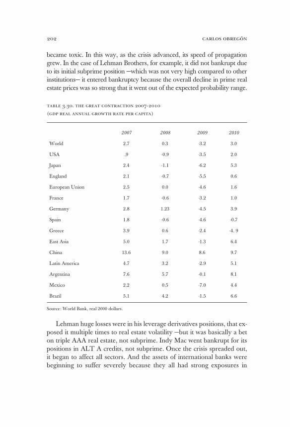
carlos obregón202
became toxic. In this way, as the crisis advanced, its speed of propagation grew. In the case of Lehman Brothers, for example, it did not bankrupt due to its initial subprime position —which was not very high compared to other institutions— it entered bankruptcy because the overall decline in prime real estate prices was so strong that it went out of the expected probability range.
table 3.30. the great contraction 2007-2010
(gdp real annual growth rate per capita)
2007 2008 2009 2010
World 2.7 0.3 -3.2 3.0
USA .9 -0.9 -3.5 2.0
Japan 2.4 -1.1 -6.2 5.3
England 2.1 -0.7 -5.5 0.6
European Union 2.5 0.0 -4.6 1.6
France 1.7 -0.6 -3.2 1.0
Germany 2.8 1.23 -4.5 3.9
Spain 1.8 -0.6 -4.6 -0.7
Greece 3.9 0.6 -2.4 -4. 9
East Asia 5.0 1.7 -1.3 6.4
China 13.6 9.0 8.6 9.7
Latin America 4.7 3.2 -2.9 5.1
Argentina 7.6 5.7 -0.1 8.1
Mexico 2.2 0.5 -7.0 4.4
Brazil 5.1 4.2 -1.5 6.6
Source: World Bank, real 2000 dollars.
Lehman huge losses were in his leverage derivatives positions, that ex-posed it multiple times to real estate volatility —but it was basically a bet on triple AAA real estate, not subprime. Indy Mac went bankrupt for its positions in ALT A credits, not subprime. Once the crisis spreaded out, it began to affect all sectors. And the assets of international banks were beginning to suffer severely because they all had strong exposures in

203a new look at the 2008 crisis
their books to USA’s assets. Those developed countries that had a more internationalized banking system were more affected by the credit crisis. And their credit crises, in turn, produced credit crises in other countries to whom they lent regularly —like Greece.
The fourth mechanism of transmission occurs because the credit crisis reduces global demand for real estate and therefore deflates real estate price bubbles in those countries that have had a real estate boom. The fall of these real estate prices initiates negative feedback circuits within these countries.
According to the transmission mechanism that they were exposed, the countries were more or less affected by the great contraction of 2008. The most affected were those countries where the real estate price bubble burst, and did not have an autonomous monetary policy. Because, in ad-dition to the internal contraction produced by the bursting of real estate prices, these countries received the exogenous shock of low world growth and a fall in the global credit level; and they could not adjust to these ex-ternal shocks by a devaluation that encouraged their exports and reduced their imports. We will return later to this point.
Table 3.30 shows the consequences of the global financial crisis in the GDP per capita annual growth rate in diverse regions and countries. As can be seen, the crisis has been more acute in the developed world, since it is the most financially interconnected. Europe, that initially believed the USA crisis was not its concern, suffered a great contraction. European regulators that had distanced themselves from the markets did not under-stand was happening in the real financial world of their own economies. In hindsight, it is unbelievable that they had not appreciated the enor-mous interconnection of their financial system with the USA’s banks. But European policymakers, as the Americans, held two erroneous concep-tions: the first is that markets are self-regulating; the second is that real es-tate booms should not be a subject of concern for financial authorities. To these two misconceptions, the European policymakers added a third one of their own: that what happened in the USA in the subprime market was not their concern. The crisis and the speed of its contagion have shown us all —with clarity— how wrong were these three conceptions. The late intervention of the European financial authorities and the insufficiency of their measures had great costs for Europe. Among them, the economic imbalance of the weaker countries of the community, like Greece.
There were diverse cases within the European Union. Germany had a strong position: it had a current account surplus, it did not have a real estate boom, and the monetary policy of the Central European Bank fitted well

carlos obregón204
with what the Taylor’s rule would recommend. In the case of France, the monetary policy also fitted reasonably well with the Taylor’s rule, but it had a current account deficit and a real estate boom, so it was more impacted than Germany by the crisis. England had a tight monetary policy in relationship to the Taylor rule, but a significant deficit in current account, a banking system heavily interlinked with the USA, and a very strong boom in real estate. So that of the three major European countries, it is the most affected by the crisis.
The strength of the crisis in Japan and Mexico was due to their strong trade dependence with the United States.
The underdeveloped countries had a much less developed international banking system, and therefore were not so much subject to the credit crisis (with exceptions, like those in the European Union). The strong growth of these countries in relation to the developed countries confirms our the-sis that the true detonator of the crisis of 2008 was the credit crisis in the developed world. Several of the least interconnected countries in the inter-national financial circuit had their own real estate price bubbles, but these did not break out, and did not produce a sharp drop in GDP. Among the countries that had real estate price bubbles, but resisted the crisis well were China, Russia, Argentina, South Korea, and India.
The problems of the European Union and the case of Greece
The crisis in Europe has been deep and long. The reason is to be found in the structural problems of the European Union. The central problem of the Euro-pean Union is that it is a monetary union that has had problems from its con-ceptualization. It is not theoretically feasible to have a single currency without two other fundamental conditions: free migration and a common fiscal policy.
The first condition is not fully satisfied in the European Union par-tially due to the differences of languages, but mainly by the great distance between the levels of education and of professional abilities specific to the different countries that make up the Union. The second condition is simply not met; policies aimed to have certain common rules regarding fiscal policy in general have failed. As can be seen in Table 3.11, the mon-etary policy of the European Central Bank is approximately similar to the Taylor rule for Germany and France, but it was very accommodating for other European countries, such as Spain and Greece. The consequence
205a new look at the 2008 crisis
has been a very divergent behavior, economically speaking, between dif-ferent countries of the European Union.
The basic problem of a monetary union is that it greatly restricts the possibilities of adjustment to an exogenous shock. Essentially this was the problem of Greece. In what follows, we will discuss the Greek example because it illustrates very clearly the economic problems of the European Union.
Let us see what the position of Greece was. It had an accommoda-tive monetary policy that was not balanced by a restrictive fiscal poli-cy, but on the contrary, it had a very large fiscal deficit. Thus, before the crisis, Greece had a large current account deficit and a real estate boom, even if not as pronounced as Spain’s. The consequence was that the crisis affected Greece seriously, as can be seen in Table 3.31; but initially less than Spain, because Greece heavily expanded public spending. However, for 2010, Greece entered a crisis of growth much more profound than that of Spain. Why? Because Greece entered into a huge credit crisis. As a result of the 2008 crisis, its external debtors were not willing to continue to finance Greek growth based on exter-nal indebtedness; that already looked very unsustainable before 2008. When external indebtedness stops, Greece enters into a serious credit crunch, and the GDP collapses in 2010.
What would normally be the solution to an economic growth prob-lem of such dimensions? If we speak of developed countries, the solu-tion is to expand aggregate demand by incurring into a large public sector deficit and a significant money supply expansion. Exactly what the United States did. These measures that expand aggregate demand when GDP is contracting are called anti-cyclical policies.
For underdeveloped countries, the IMF has generally recom-mended pro-cyclical economic policies —exactly the opposite of what the USA did. Why? The argument of the IMF is that there is no confidence in the underdeveloped country. Therefore, if the aggre-gate demand increases substantially via an expansionary monetary policy and an increase of the public sector deficit; the larger current account deficit will provoke an investors run-out, which will quickly force a mayor devaluation. To avoid this scenario, the IMF recom-mends pro-cyclical policies —for which it has been harshly criticized, among others by Stiglitz— but the truth is that the IMF lacks the resources to sustain an anti-cyclical recovery program of an under-developed country.

ca
rlo
s o
br
eg
ón
20
6
table 3.31. greece: crisis economonic indicators
Real GDP
(annual %)
CPI
(annual %)
Balance of payments (GDP
% )
Government
net position GDP %
Gov. debt (accumulated
GDP % )Unemployment
2001 4.2 3.7 -7.2 -4.3 81.2 10.8
2002 3.4 3.9 -6.5 -4.8 85.5 10.3
2003 5.9 3.4 -6.6 -5.7 97.3 9.7
2004 4.4 3.0 -5.9 -7.4 98.8 10.5
2005 2.3 3.5 -7.4 -5.3 100.3 9.9
2006 5.2 3.3 -11.2 -6.1 106.1 8.9
2007 4.3 3.0 -14.4 -6.7 105.4 8.3
2008 1.0 4.2 -14.7 -9.8 110.7 7.7
2009 -2.3 1.4 -11.0 -15.5 127.0 9.4
2010 -4.4 4.7 -10.4 -10.4 142.0 12.5
2011
(IMF forecast)
-5.0 2.9 -8.4 -8.0 153.0 16.5
Source: IMF. World economic Outlook database https://www.imf.org/external/1pubs/ft/weo
207a new look at the 2008 crisis
So, even though technically Stiglits is right, it is not really a problem that the IMF can solve; it must be solved by the developed countries —but the developed countries have been reluctant to give the guarantees that would be required to sustain anti-cyclical recovery programs in the underdeveloped countries. Each one of them fears that if it supports an underdeveloped country, the benefit of the recovery will not benefit it (the guarantor), but it will benefit some other country that has not risked anything to support the underdeveloped economy’s recovery. It is a clas-sic game theory problem.
The IMF adjustment programs policies are: to restrict the money sup-ply, to reduce public spending, devalue the currency, privatizations, free trade and free internal markets, structural reforms of the labor market, and raising real interest rates.
The consequence of these adjustment programs is a sharp decline in nominal and real GDP that reduces imports —which are also reduced via the devaluation. Finally, the devaluation increases exports and allows the substitution of imports. This new growth path substantially complements the endogenous recovery of growth, and the country begins to grow; it becomes reliable again and returns to international credit (the one that never came before, when it was really need it). The IMF programs are successful, but harsh on the population of the underdeveloped countries.
What is important to emphasize from the previous history is the pow-erful aid that the devaluation provides by reducing the imports and in-creasing the exports. In the traditional IMF model, devaluation brings with it an automatic reduction of the local wage in terms of the foreign currency, and this encourages exports. It is often impossible to control the inflation that is produced by the most expensive imported goods, which helps to lower the local real wage even more. Devaluations help re-duce imports because they become more expensive. Both factors–exports grow and imports decay —contribute powerfully to the recovery of local production. Devaluations are essential to reduce the impact of exogenous shocks on output and national income.
If there is no devaluation, there are only two ways to recover the ex-ternal balance and generate credible income to repay the debt. The first is to stimulate exports by lowering the nominal wage, which is socially unacceptable. The second is to lower imports through draconian GDP reductions, which implies a deep recession with great social discontent. If it had been able to devalue its currency, Greece would not had suffered a recession as deep as it did. Greece, without its own monetary policy and
carlos obregón208
without being able to devalue, is completely at the mercy of the goodwill of its neighbors to continue to lend to it–but of course, this has the same limits as always, no one wants to risk their money with the underdevel-oped country until it proves that it is credible. But for Greece, it will be very painful to prove that it is credible without being able to devalue.
There has been a real confrontation between the interests of the common Greek citizen and the interests of powerful European coun-tries, such as Germany and France. Street conflicts in Greece had been a manifestation of the above. The IMF adjustment programs have al-ways been proven unacceptable and have often triggered social unrest, which we can only expect to be much more intense in a country that cannot devalue. Greece had suffered a much higher wage adjustment and a much deeper recession than was necessary.
Greece reveals at once the contradiction of the European Monetary Union–it just does not work. It would be more advisable for Europeans to think of developing within Europe a model like Bretton Woods, with multiple currencies and fixed exchange rates to achieve what the European Union seeks, but with the possibility of devaluing when it is indispensable–as has been the case with Greece —and with more extensive and consistent international support. For further discussion in this topic see chapter four.
The European Union does not have the correct economic model to foster a reasonably quick recovery, so it will probably take many years more to get to a sustainable adequate growth path. Thus, the world economy’s current situation remains delicate, but this will be the topic of the next chapter.
The next two sections are written for the theoretical inclined readers; others may skip them and go directly to the conclusion of this chapter. The first one discusses the concept of risk and shows how it is related to the 2008 crisis. The second one discusses the characteristics of a credit economy and uses them to describe what happened in the 2008 crisis.
risk is more than just volatility
Defining risk as volatility was a great contribution of contemporary economics and finances. It produced profound changes in the financial world, such as pension funds investing in the market indexes, the fast de-velopment of the derivatives market, and the Modigliani-Miller theorem —which is the basis for modern thinking about capital structure.
209a new look at the 2008 crisis
However, despite its many contributions, the view of risk as volatility is also responsible for the rapid contagion occurred in the 2008 finan-cial crisis and for the regulators’ lack of response. Regulators thought that markets could manage risk properly because it was volatility, and therefore it could be known and could be handled by the market. They were wrong. Risk is more than just volatility, and the markets can only manage themselves properly if the governments provide the adequate institutional arrangement.
In what follows we will address the differences between the contem-porary vision of risk as volatility, and the Knight-Keynes vision of risk as uncertainty related to the unknown future. We will argue that both visions are needed, that they are complementary to each other, and that one of the reasons of the crisis is contemporary economists and regula-tors wrongly disregard of the Knight-Keynes vision.
Knight and Keynes
Frank Knight —a leading professor at the University of Chicago in the first half of the twentieth century— defined risk as non-probabilistic uncertainty, as the unknown. According to Knight, this is the type of risk that will char-acterize the future. John M. Keynes —the most important economist of the first half of the twentieth century— based his General Theory on this type of uncertainty and used it to explain The Great Depression103. In Keynes, risk is not based on a known probability function. For him, uncertainty has to do with a state of confidence regarding the future, and has precisely the function of being able to understand how events like The Great Depres-sion or The Great Contraction can happen. Uncertainty in Keynes is the centerpiece of both his theory of liquidity preference and his marginal ef-ficiency of capital. Therefore, Keynes’ uncertainty cannot be reduced to a probability function based on what we do know, as Tobin did104.
103 Mervyn King in his new 2016 book calls it radical uncertainty and argues for the enorme-ous relevance that it has to understand real economies and financial markets. See for ex-ample pages 151- 155.
104 We must not confuse future uncertainty with psychological irrationality, as Shiller and others have done. In an economic boom, economic agents do not ignore that houses are ex-pensive in relation to incomes. They read the newspapers, and do not ignore that the interest rates are unusually low, and they do not process the information irrationally. They have the information and they process it rationally–i.e. according to a rational expectations model. But
carlos obregón210
The three great contributions of defining volatility as risk
Keynes and Knight’s view of uncertainty as that which is unknown was replaced by postwar economists with the notion of a probabilis-tic risk based on information of what is known. This transformation had great consequences in the history of macroeconomics and finances. This is initially due to the 1981 Nobel Prize winner, James Tobin. In his initial contribution to the theory of the portfolio in 1956, Tobin argues that the reason people diversify their portfolio between bonds and cash, although the cash does not have any return, is because there is uncertainty in relation to the future rate of interest. Cash is a way to protect yourself in the event that interest rates rise and the bond posi-tion becomes a loser. To measure this future uncertainty, Tobin uses a probability function.
Thus, curiously enough, in an article in which it appears that Tobin is enriching Keynes’s theory, he actually disappears Keynes’ uncertain-
that does not mean that what is rational for them is not to buy because they have identified a boom. The key is to understand the notion of real time (in which Shackle always put a lot of emphasis). To know that, in the end, the real estate will return to a rational average in terms of its replacement cost (construction cost) does not solve the problem of when it will happen. The models run in an abstract time, different from the historical-time in the real world where economic agents live and die. Economic agents do have an age. In this way, even taking all the information and using it rationally —having the best model— it is rational to buy a good that is expensive, simply because what is not known is how much more expensive it will get in the real period that is of interest. Economic agents do not buy the house without calculations and only guided by their irrational emotions. They make calculations rationally, and there is nothing wrong with using a rational expectations model to reproduce what people do. But the model has the limitation that it cannot forecast when in real time will the boom end. It cannot reduce future uncertainty. Take the example of Microsoft, no rational expectations model would have predicted what happened. The acquisition of this company, as of others, implies an optimistic vision of the future. If it goes well, then it is said that the economic agent had a great vision; if it goes wrong, is argued that it was irrational.In the face of uncertainty, we act. Booms have logical reasons to develop. The economic boom may continue for many more years or not, nobody knows. The real estate boom could have lasted longer. Real estate prices in general, even when already high, were not the reason for the crisis. It was not irrational for participants to buy at high prices, like Shiller had argued. Real estate in Europe was much more expensive. Participants in the subprime boom could not have predicted that interest rates would go up as rapidly as they did. Even professional market participants did not predict it. If someone could do this kind of predictions, with cer-tainty, they could become inmensely rich. Even using the best rational models, no body can predict for how long a market would remain overvalued or undervalued —adjustments may take decades. Economic agents buy in a boom not because they act irrationally, but because there is future uncertainty and it makes decisions very difficult. That you must make decisions in a world with uncertainty and real time does not mean that you are irrational in taking them.
211a new look at the 2008 crisis
ty theory from contemporary discussion. Tobin was successful, to the point that the great majority of the postwar economists have not read thoroughly Keynes’ General Theory.
From the point of view of finances, Tobin’s conception of risk had great consequences. Tobin’s notion joined that of Harry Mar-kowitz, who had already written that investment portfolios had to be diversified, and that the risk of the total portfolio could be measured through the covariances of the shares it contains. Tobin suggested that the decision between risk-free and risky assets could be done with his portfolio theory, and that risky assets could be selected using the Markowitz methodology that maximized performance for a given risk level. Markowitz’s efficient frontier is the set of all portfolios that will deliver the highest expected return for each given level of risk. These concepts of efficiency are essential for the development of the Capital Asset Pricing Model (CAPM) model, developed later on by William Sharpe, a student of Markowitz’s, who shared the Nobel Prize with him in 1990. CAPM proposes a systematic methodology to maxi-mize return, minimizing total portfolio risk. It is based on the covari-ances between the assets.
Sharpe proved that the most efficient portfolio of all, the one opti-mizing risk-return, is the portfolio that buys the entire market. Sharpe’s result forever changed the professional investment fund management industry. Pension investment funds increasingly acquired the total stock market index. This was the first great contribution of the defini-tion of volatility as risk.
Franco Modigliani (Nobel 1985) and Merton Miller (Nobel 1990), would also use the efficiency of the markets to show their theorem —that establishes that the value of a company is independent of its capital structure, i.e. it is independent of whether the company uses capital from its shareholders or market debt. The Modigliani-Milller theorem is the basis for modern thinking about capital structure. This is the sec-ond critical contribution of volatility as risk.
Fischer Black and Myron Scholes (Nobel 1997) would also use the markets’ efficiency to show that the price of a derivative is independent of the price of the underlying asset, and depends only on the underly-ing asset’s volatility. All things being equal, the theoretical value of an option is a monotonous increasing function of implied volatility. The derivative market changed forever the practice of finance. This is the third enormously important contribution of defining volatility as risk.
carlos obregón212
The macroeconomic consequences of defining risk as volatility
From the point of view of macroeconomics, Tobin’s demand for money replaced Keynes’ liquidity preference and was incorporated into the IS-LM model, initially proposed by Sir John Hicks (Nobel Prize 1972). Pre-viously, Hicks had eliminated Keynes’ marginal efficiency of capital and had introduced his own investment theory related to the interest rate. The result is that Keynes’ conception of uncertainty and the two theoreti-cal pieces he used to understand the macroeconomic consequence of such uncertainty disappeared from the economic literature. Which in retro-spect was a shame because these two pieces were the key to understand the Great Contraction’s origins and why it has lasted so long —despite the mega-cannon money injected by the Central Banks.
The IS-LM model was used as a theoretical basis for the Keynesian-Monetarist controversy, which was discussed using the empirical data of the American Economy as evidence; which throughout the second half of the 20th century remained very close to equilibrium. Finally, the stagflation gave the definitive triumph to the monetarists. Monetarism became ratio-nal expectations and the centerpiece of the macroeconomic thinking of the main tradition. But the point is that these controversies left aside the kind of problem that Keynes had visualized with the General Theory —The Great Depression. The IS-LM model was used to develop growth models with en-dogenous expectations and differential equations to simulate and understand economic cycles. The consequence of endogenizing expectations was that the way was opened to what would eventually become Rational Expectations. In this way, both economic theory and the empirical reality of the United States reinforced the view that markets were self-regulating.The Great Depression became historically distant; the world economy since Bretton Woods was stable. Therefore, the post-war financial crises were seen as a characteristic of the developing countries, consequence of their institu-tional weaknesses. The developed world was conceived as in equilibrium. Lucas, Nobel Prize in Economics and the main exponent of the school of Rational Expectations, wrote that Keynes’ theory was already dead. Rational expectations theory is based on the assumption that all economic agents use rationally all available information and argued that economies, if left alone, are brought to equilibrium by the market’s dynamics. Rational expectations were the theoretical frame that better explained the stagflation phenomenon. But, despite Lucas’ dictum, the 2008 crisis brought Keynes back.
213a new look at the 2008 crisis
The problems of defining risk as volatility
Measuring volatility requires historical observations, therefore depends on the specific historical period used. To minimize this bias, analysts typi-cally use a reference period as long as possible —though this does not take away its historical dependence.
One of the recent failures in the use of this type of risk estimates was the famous Long Term Capital Management (LTCM) fund that had the advice of Nobel Prize winners in economics, and the financing by the big USA banks. The LTCM fund developed risk models to invest in Russia. Nevertheless, the Russian crisis of 1998 brought great losses to the LTCM fund. Why? Because the crisis did not behave like the historical past. There is really no way to know the future through prob-ability models.
The basic reason for Lehman Brothers’ bankruptcy was that the vola-tility of the markets did not behave like anything they had seen in recent history. Lehman’s risk models failed, and Lehman broke eventually. The risk ultimately turned out to be something different, something more than just volatility. Volatility risk as defined by the various Nobel Prizes that studied it (such as Tobin, Markowitz, Sharpe, and others) cannot explain the 2008 crisis. Knight and Keynes were right after all. Unfortu-nately, their thinking was not followed by the main tradition because the economy of the developed countries took, after the 30s, eighty years to register a new global financial crisis.
The derivatives market and the 2008 crisis
The derivatives, as discussed, relate to the volatility of the underlying asset and there may be many derivatives in any type of asset (i.e. many positions on the future volatility of that asset). It is important to distin-guish between Futures and Options. Futures: A futures contract is simply established for the future purchase or sell of an asset at a preestablished price; example, Swaps, in which the characteristics of one asset are ex-changed for those of the other (i.e., an interest rate swap exchanges the future flows of interest rates of one asset for another). Options: there are very different types of options, but the two fundamental ones are the call

carlos obregón214
and the put. Buying a call means the right to be able to buy the asset at a future fixed price (it differs from the future in that it is only the right, but not the obligation to buy it). Selling the call means giving the right for another to buy it. Buying a put means the right to be able to sell the asset at a certain price. Selling the put means giving the other the right to sell the asset at a certain price.
Derivatives can be sold and bought on the stock exchange and then be named Exchange Traded (ET), or they can be exchanged by two counterparts privately and called Over the Counter (OTC).
It is necessary to distinguish between the notional value of a deriva-tive and the gross market value. The notional value is that established in the contract; the gross market value is what the instrument would have if it were settled at this time. The gross market value is the one that would be comparable, for example, to the value of a company’s stock or the value of a house —it is the value of the derivative itself. However, since the value of derivatives is based on volatility, it is necessary to maintain the notional value as a reference. This means that the market value of a derivative can change abruptly if we move outside the traditional equi-librium of the markets —outside historical volatility. This is exactly what happened in 2008.
Most ET derivatives are interest rate swaps (futures) or interest rate options —which, in general, do not present a systemic risk and they were not those that triggered the concern in 2008. A large part of the OTC derivatives is also interest rate swaps that do not present systemic risk either. Nevertheless, the OTC includes the Credit Default Swaps (CDS), —including those securing the payment of mortgage loan pack-ages (CMOs - Collateralized Mortgage Obligation) — which can produce systemic risk, and they did in 2008.
In 2007, before the crisis, the gross market value of the global de-rivatives market (excluding interest rate swaps) was 8.6 trillion dollars —around 5% of the total value of all financial assets worldwide. Of the 8.6 trillion, the CDS represented 2 trillion. In 2008, the CDS went up to 5.1 trillion. Why did they go up so much? Because of systemic risk, when it occurs, risk changes are parametric. This is what drove AIG (the most important insurer in the United States) into bankruptcy.
Derivatives are the price of volatility, therefore, if volatility gets out of its historical trend and increases a lot, the derivatives price can move sharply. The gross market value of the CDS in 2007 did not include the systemic risk that materialized in 2008. Here we have a clear example of
215a new look at the 2008 crisis
the two type of risks we have been discussing. What was in the value in 2007 was historical volatility risk; the value in 2008 was volatility risk plus systemic risk —institutional risk, the risk of the unknown future, people did not know what was going to happen, that is why the CDS value moved so sharply.
What is risk?
Who is right, Tobin or Keynes? Is it okay to use volatility as a measure of risk? Why did the value-at-risk models based on volatility (VAR) failed? Is it possible that so many Nobel Prizes are wrong?
There are clearly two very different visions about what is risk: 1) for Knight and Keynes, risk was uncertainty related to the unknown; and 2) for the postwar economist of the main tradition, risk was volatility. The two visions belong to two different conceptions of the economic world, constructed to explain different real economic situations. Keynes was concerned about explaining how situations such as The Great De-pression and the Great Contraction can arise. Postwar theorists were concerned about understanding the near-equilibrium economy that was experienced in the second half of the twentieth century. It is not the case that one vision of risk is correct and the other is wrong. In fact, they complement each other and are useful to explain distinct circumstances of the economic reality.
The notion of equilibrium is necessary to obtain contemporary fi-nance theories’ results. If the economy is close to equilibrium, historical volatility is a good indicator. Consequently, the three great contributions of risk as volatility do hold up. Derivatives markets work well, investing in the market as a whole is good advice, and it does not really matter whether a company is financed with equity or not. However, if we move away from the equilibrium, the results of finance theories no longer hold up because historic volatility is no longer a good indicator. This is what happened with the LTCM fund or with Lehman Brothers.
Neither of the two visions is wrong, they just explain distinct realities. Depending on the type of problem we are going to solve, one vision or the other may be more appropriate. Both visions could be complementary. But what is certain is that postwar economist and regulators had totally disregarded the Knight-Keynes vision. The consequence was that in the

carlos obregón216
2008 crisis the market participants’ conception of risk and of the regulators was only based on the vision of risk as volatility. Therefore, when the 2008 credit crisis occurred and produced unusual large volatilities —for historical standards— the financial market collapsed, because the risk models used could not contemplate volatilities so distant from the historical ranges.
The concept of risk as volatility is only sustainable in an economy close to equilibrium in which the future does not differ substantially from the past. The basic concept of VAR models is that the value at risk is related to the historical volatility of the investments made, particular to their covariances. When there is a generalized collapse of confidence, we move from the world of equilibrium to the world of Knight and Keynes and historical volatility ceases to function properly as a guide for the fu-ture —this is what happened in 2008.
A theoretical framework
Minsky modifies the money demand of the IS-LM model to make explic-it the precautionary demand of money; in the IS-LM model, the demand for money is given by (1) and in Minsky by (2) as shown:
(1) Ld = Ld (y, p)(2) Ld = Ld (y, p, Pk, F, NM)In this case, y is national income, p is the deposit interest rate, Pk is the
price of capital goods and introduces the uncertainty associated with its possession, F is the precautionary motive for possession of Money and NM quasi-money, which can also be used to satisfy the precautionary de-mand for money. For Minsky, the key is that the price of real capital as-sets in relation to financial debts depends on U (the state of uncertainty). In a recession, when the money supply goes up and p goes down, the debt capitalization rises and Pk should also rise, but if U deteriorates, then Pk does not go up enough. The balance of the companies deteriorates; given their higher risk, banks raise their margin and r (the bank lending rate) rises, or banks ration the credit, or a combination of both. Note that in this recessive process there is an increase in real balances because of the fall in prices and monetary wages, and that this stimulates consump-tion (the neoclassical effect). But Minsky’s point is that the effect of the increase in the companies’ debt (and we would add the consumers’, con-sequence also of the fall in prices and wages), can more than offset the effect of the real balance sheets’ increase.
217a new look at the 2008 crisis
Summarizing the previous model, the distinctive feature of a credit economy is that it depends on the state of confidence U, on uncertainty, on the vision of the economic agents’ future. If the state of confidence de-teriorates, assets whose value depends on the vision of the future (in the case of Minsky, capital goods) lose their value, the balance sheet of the agents that own them deteriorates, the banks restrict credit and the dif-ferential between the central bank rate and the lending rate of the banks rises. Then negative feedback loops are unleashed.
Minsky’s model does not include consumers nor parallel banking, but it is relatively easy to see how it would operate in this case. Parallel bank-ing is more willing, and able (because it is less regulated), to take higher risk so that they should reduce their credit less, thus, taking the route of significantly higher lending rates. Consumer’s long-term assets, such as their home and their investments in the stock market, also look into the future. Therefore, the consumer’s accumulated wealth (net worth) also goes down. In a recession, when the central bank rate goes down the stock market should rise, but given the little confidence in the future, U deteriorates and —consequently— the stock market, instead of rising, goes down. The same happens with real estate, but nominal consumer debts are maintained. Hence, the balance of the consumer deteriorates, this leads to the reduction of bank credit, r rises, and a negative feedback loop is unleashing. That is exactly what happened and that is why recovery has been so slow. In a credit economy, monetary policy is not as effective as it is in a traditional macroeconomic model. That is why Bernanke had to use heterodox policies.
Minsky’s, Wicksell’s, and Stiglitz’s & Greenwlad’s (2003) models em-phasize the decline in the supply of credit as a result of the deterioration in the balance sheets of credit claimants. The Stiglitz & Greenwald model has the advantage of its more elegant and precise mathematical formaliza-tion, but it operates in a similar way to Minsky’s105. These authors point out that the objective of monetary policy is not p but r. If r rises above the desired equilibrium —if in a recession r is contractionary rather than stimulating— the central bank must lower p even more and reduce the required reserves. This task is difficult if parallel banking is widespread, as the central bank has little control over it.
Minsky’s model makes an explicit description of the demand for money that is not in Keynes’s work, but is compatible with the view of this author. In Keynes, Minsky, and Stiglitz & Greenwald, finan-
105 For a summary of this model, see Obregon 2008a.
carlos obregón218
cial relations are given in nominal terms. Keynes criticizes Fischer106 because Fischer distinguishes between the nominal interest rate and the real rate, but does not distinguish whether future changes in the value of money were anticipated or not107. Thus, for Keynes, Fischer’s theory is written based on a real interest rate that would have to prevail “as a result of a change in expectations about the future value of money, so that this change has no effect on the cur-rent product”108. The distinction of Minsky and Stiglitz & Greenwald between p and r is very compatible with Keynes’ original thinking on the preference for liquidity.
But Keynes goes further because, besides the preference for li-quidity, he introduces the marginal efficiency of capital rd, the dis-count rate used by investors to discount the future. If rd is very high, it means that investors are very concerned about the future. Thus, in Keynes, two mechanisms slow economic recovery and hinder the effectiveness of monetary policy. The first is the preference for li-quidity: the contraction of bank credit and the rise in the lending rate of banks. The second is the rise in the marginal efficiency of capital. According to Keynes, uncertainty is reflected both in the preference for liquidity and in the marginal efficiency of capital. The first maintains r too high and/or reduces credit amounts, and the second rises rd.
In Keynes, the demand for credit and the supply of credit can determine r and the amount of credit, but not rd. The lack of credit may be a problem for investment, but the presence of credit does not necessarily solve the investment problem since rd is defined by the uncertainty associated with expected future flows. This is why, despite Bernanke’s heterodox policies, the economic recovery has been slow.
With this background, we can see with theoretical clarity why it has been so difficult for Central Banks to stimulate the economy. 1) Central Banks have control over p, but not a good control over r (and with the growth of the parallel banks, have been losing control over monetary aggregates), 2) and even if they manage to influence r, they have no control over the demand for credit and over rd. What
106 A point Patinkin did not understand
107 Keynes, quote in Obregon, 1989, p. 173
108 Idem
219a new look at the 2008 crisis
Bernanke brilliantly did was to understand that he needed to sustain asset prices by buying them directly, which was equivalent to lower r.
In Keynes, there is also no theory that describes what happens to the consumer, but we can see that it is easy to extend the model. The con-sumer has his own discount rate of the future: let us call it, rdc. Thus, even if the Central Bank manages to influence r, it is possible that the economy recovers slowly because rdc and rd remain too high. There-fore, if we compare what had happened in Japan before with what hap-pened in the USA after 2008, the difference is that, due to Bernanke’s heterodox policies, the USA was able to influence r, which Japan never managed to do. This is why recovery happened faster in the USA than in Japan. Still, Bernanke’s large purchases of assets did not influence rcd and rd, that is why the US recovery —despite being faster than Japan’s— was also slow.
How does this model of credit economy work in the great contraction of 2008?
The crisis of 2008 begins with the banks’ credit crisis, confidence in the future U deteriorates. Then, at first, the supply of credit is reduced (the supply curve shifts to the left). Later, as the credit quality of credit clamors is getting worse, besides continuing to reduce the supply of credit, it is also becoming inelastic (insensitive to changes in p). Finally, the demand for credit itself is reduced because of rd and rdc rise (the demand curve also shifts to the left and becomes inelastic). At first, with the reduction in the supply of credit, r rises; then, with the fall in demand for credit, r tends to decline. The final result on r is indeterminate. But, what we do know is that the total amount of credit is reduced, and that the new LM (for those who are economists) is inelastic (insensitive) to both changes in p and r.
With the rise of rd and rdc, both investment and consumption fall and become insensitive to changes in p and r (for economists, the IS shifts to the left and becomes inelastic).
With the shift of LM and IS to the left, the aggregated demand is reduced, and as a consequence of the inelasticity of both curves, the ag-gregate demand becomes inelastic, making the Central Banks’ task to recover the economy more difficult.
The consequence of the above is that total credit falls, credit on GDP is low and GDP growth is low, exactly what happened in the Great

carlos obregón220
Contraction of 2008. As can be seen in Table 3.32, total credit fell 42% in 2008 and was negative in 2009. Credit granted by financial institutions fell in 2008 23.2% and was also negative in 2009. These brutal declines in credit reduced it to GDP and led to GDP declines of -0.3% in 2008, and -3.5% in 2009. The theory fits perfectly with what happened in real-ity. That the credit crisis was still present in 2010, the total credit flow represented only 12.3% of the flow in 2007, and the flow of credit from financial institutions was still negative.
table 3.32. total credit in the market-loans (flow billions of dollars)
Total loans Loans created by financial institutions
2006 4 040.9 2 854.0
2007 4 482.3 3 055.7
2008 2 580.9 2 384.1
2009 - 606.6 - 843.2
2010 553.0 - 279.9
2001(2t) 704.9 939.7
Source: Federal Reserve, flow of funds, Table F1.
What happens to fiscal policy in the great contraction?
In principle, fiscal policy has the great advantage of increasing aggre-gate demand directly, and does not have the problem of traditional monetary policy, which with the uncertainty of the future (U, rd and rdc) does not work properly. Even Bernanke’s large purchases of as-sets, given the uncertainty of the future (rd and rdc) work slowly. Yet, Keynes himself warned us that, while he knew that monetary policy in an environment such as The Great Depression had difficulties in recov-ering the economy, he was not sure that fiscal policy could solve the problem. Why? Because the government cannot replace the private sec-tor. Government demand lacks the main virtue of the capitalist system, the consumer preferences’ transmission in an efficient way through the price system. The government’s task to regain private sector confidence may or may not be successful and if it is not, government spending will
221a new look at the 2008 crisis
only nationalize parts of the economy rendering them inefficient. Thus, not only it is necessary to expand government spending (since mone-tary policy has limitations), it is also essential that government spending be directed towards re-establishing the confidence of the private sector, which was not well done in the USA.
What policies were needed?
The basic problem of the economy in 2008 was the lack of condidence in the future as a result of the deterioration in financial agents’ balance sheets. Thus, the main policy goal of the government should have been to regain confidence, raise U. Government spending should have been directed first of all to clean up those balance sheets; it was of paramount importance to have withdrawn the toxic assets of the banks at an early stage.
In addition, the government’s objective should have been to restore confidence in the proper functioning of the private sector. Therefore, it was unwise to launch such widespread criticism of the private sector’s conduct. The more it was announced that the private sector was mal-functioning, and that there were irresponsibility problems in the balance sheets of many financial agents, the more U deteriorated, and the worse the credit economy was.
Without a policy to reestablish economic agent’s healthy balance sheets, it was not possible to achieve economic recovery soon. Capitalism without a properly functioning financial system simply does not work. Hence, the government’s main objective should have been the long-term restructuring of all economic agents’ balance sheets so that U would re-cover, and the credit economy could have been put to work. That is why events like the mismanagement of Greece’s case by the European financial authorities was so disturbing for the world economy because they raised U —the distrust in the ability of the credit economy to func-tion properly.
Another goal policy for the government is to influence rd; to do this, the government has to ensure that the private sector firmly believes in the economic recovery. Government spending has to go directly to projects that involve increases in private sector investment —seeking joint ven-tures is very important. The government with its spending should lead the recovery of private investment, not replace it.
carlos obregón222
As we mentioned, the government should have entered early on in the crisis to rescue the toxic assets in order to avoid the deterioration of rdc. However, once it was deteriorated, the policy goal should have been to recover rdc. This is a very difficult task and has much to do with the proper management of social communication. It was not wise to keep tell-ing the consumer that he was irresponsible for getting into so much debt. The consequence has been that convincing the consumer to increase his consumption and his debt levels has become a very difficult task. Due to this, recovering consumer confidence has been an extremely slow process.
Bernanke’s heterodox policies were very successful because he influ-enced r directly with his large asset purchases. If he had not done so, tra-ditional monetary theory would have helped very little, as the previous experience with Japan taught us. Anyway, the USA economic recovery has been much slower than it could have been, for three reasons:
1. The required early policy to consistently get rid of the toxic fi-nancial assets was never implemented. This policy could have avoided both the deterioration of the economic agents’ balance sheets and the deterioration in rdc and in rd.
2. Public spending did not involve massive alliances with the pri-vate sector, and therefore was not very efficient in raising rd.
3. There was not a proper communication policy to regain con-sumer confidence gradually- ie to raise rdc.
conclusion
The vision of risk as volatility gave rise to a big revolution in both financ-es and economics. The big innovations that followed changed forever the financial markets, such as the derivatives market, the indexed funds industry, and the Modigliani-Miller theorem —which is the basis for mod-ern thinking about capital structure. Despite all its success, there were unwanted consequences in the introduction of the vision of risk as vola-tility. Risk began to be thought as endogenous and capable to be known probabilistically, therefore the role of institutions as a bridge between the present and the unknown future was disregarded.
Tobin’s demand for money replaced Keynes liquidity preference and, together with the previous replacement that Hicks had done eliminating Keynes’s marginal efficiency of capital and introducing his investment
223a new look at the 2008 crisis
demand as an interest rate function, fully eliminated from macroeconom-ic-thinking Knight and Keynes’ notion of risk as the uncertainty related to the unknown future. With the economy near equilibrium for many years, economist built endogenous models and developed distinct theo-ries of expectations that finally gave raise to the School of Rational Ex-pectations, which elegantly explained why the economy is always near equilibrium. In addition —despite many theoretical advances that indicate that, in order for markets to operate properly, they need an adequate in-stitutional arrangement— regulators and market participants became con-vinced that markets regulate themselves and could manage risk properly through sophisticated probabilistic models.
The subprime crash was a consequence of the Fed drastically moving down and up the Fed’s rate. Once the subprime crash started, if the regu-lators and financial authorities have had the proper vision of risk, as in-cluding not only volatility but also the uncertainty about the future, they would have understood properly the characteristics of a credit economy. And they would have intervened to get rid of the toxic subprime loans from the banks —and the banking crisis would have been avoided. They did not do so because, as the Economic Report of the President reiterates, they were convinced that the markets were going to do a better job than they could in managing risk.
However, markets do not operate well unless they have the proper institutional framework; which does not mean overregulation, it means to be vigilant and intervene whenever is needed. But to be able to do so, regulators need the proper theoretical framework to analyze the financial economy and be very close to the financial innovations happening in the market. Regulator distant from the market, because they thought it could auto-regulate itself, and the rapid financial innovations —partially due to the new managing capacity allowed by the ICT revolution— was the worst of combinations. Financial authorities took the wrong decisions, and the consequences happened extremely fast and were huge. A minor local problem —the crash of the adjustable rate subprime loans in the USA— became a global financial crisis of unexpected dimensions.
Bernanke finally understood that he had to act beyond traditional monetary theory; he had to influence credit directly, and he did so through his large asset purchases that prevented a second Great Depres-sion. However, he entered too late, and the economy’s state of confidence respecting the future had deteriorated a lot. In terms of the last section, U had deteriorated and rd and rdc had gone up substantially. Bernanke’s
carlos obregón224
heterodox policies helped with U, but not with rd and rdc —that is why recovery has been slow.
In the postwar period, Knight and Keynes’ vision was simply forgot-ten because in the real world the economy was near equilibrium. To un-derstand what happen in 2008, we need to have a dual vision of risk. We must accept the advantages of risk seen as volatility, but without forget-ting that parametric changes —due to changes in the uncertainty as to the future— can occur. We must acknowledge that an adequate institutional framework is required for the markets to operate well. We must listen to the many prestigious dissidents that have been warning us not to rely so much on the system’s homeostasis capacity to maintain equilibrium.
Paul Samuelon (Nobel 1971) and Robert Solow (Nobel 1987) always opposed the vision of the School of Rational Expectations. In a television interview, Samuelson said: “we have created monsters”, referring to all derivatives involved in the 2008 financial crisis, such as CDS. Krugman (Nobel 2008) has also shown skepticism about the vision of an economy in equilibrium. Nash (Nobel 1994) showed theoretically that there are multiple general equilibria that are not pareto efficient. Stiglitz (Nobel 2001) showed the existence of multiequilibria based on information failures. North (Nobel 1993) warned us that the market always works within an institutional arrangement. These dissidents were not the ones who suc-ceeded in the postwar tradition; but after the 2008 crisis, we must listen to them. Keynes is not dead.
In this chapter, we have discussed why the official explanation of the 2008 crisis is wrong. The crisis was not due to global over saving and current account imbalances; therefore, there is no need to balance them. This will be one of the topics of the next chapter.
[225]
THE ICT REVOLUTION AND THE INTERNATIONAL
ECONOMIC ORDER
Capitalism and democracy were born together in the West. Democracy gave capitalism a motor engine of its own. As a result of the political triumph of the middle class we had mass production, which is the key to technological innovation, and, therefore, for economic development. The dynamic preferences of the middle class are what distinguished capitalism from communism. The USSR had high savings, high quality education, advanced technology, sophisticated science and a large market, but it did not have the middle class’ mass consumption that the West had.
As Table 4.1 shows, Europe’s 30, plus the Western Offshoots, plus 7 Eastern Europe explain most of the world’s market growth from 1500 to 1950109. In 1500, they had 32% of the global middle class market; in 1950, they had 94%. Hence, these countries as a group have had an endogenous growth —independent from the rest of the world, sustained precisely by the growth in the mass consumption of their middle class. No other previous empire could have achieved such a market expansion in an endogenous manner for 450 years as this group of countries did. To expand, previous empires had needed new conquered territories. Capital-ism expands itself endogenously because of the growth of middle class mass consumption.
However, as capitalism matures, new technologies bring markets and people closer together. This creates the fundamental contradiction of this mode of production, the one between global capitalism and national de-mocracies. The ICT revolution has accelerated globalization and has deepened the contradiction.
The two great wars were consequence of the confrontation between the national democracies’ growing global interests. But the economic and social costs of the confrontation were so high that, in Bretton Woods, a new global order is designed to ameliorate the inherent contradiction between global markets and national interests. The new global order
109 Market is defined as (World’s GDP per capita in 1990 PPP dollars minus the correspond-ing Africa’s GDP per capita)*world population, see footnote in Table 4.1.
carlos obregón226
was so successful that people had forgotten how much a global order is needed. The newborn ideologies at the end of the 70s —in a revival of neoclassical economics— defended that the economic market process naturally tends towards equilibrium. Thus, for these thinkers, what was wrong in globalization was that governments had created barriers that do not allow the global economic process to achieve its natural equilibrium. In this view, developed countries were always close to equilibrium, and underdevelopment was the result of not allowing the market forces to operate freely. The consequence was that Bretton Wood’s institutions were either dismantled or maintained with a scope of operation substan-tially reduced. The new ideologies at the end of the 70s offered a world of economic growth and stability for the West; and they maintained that those underdeveveloped countries that follow liberal policies were going to become developed, and that extreme poverty was going to disappear from the planet. Bretton Woods was substituted by the invisible global hand of liberalism.
The story told by the new liberal ideologies never materialized itself. The West ended up with the 2008 crisis. The underdeveloped countries that followed the liberal policies did not develop and the poor countries remained poor. The only countries that did develop were the ones that adopted the Asian Development Model, and these were the only coun-tries that reduced drastically the number of poor people.
The consequence of the 2008 crisis was the revival of nationalism and protectionism in the West. Such revival explains both the votes for Brexit and Mr. Trump and the growth of the right wing parties in many other developed countries —where even if they do not win the elections, they have become a much more important political player.
The failure of the developing countries that followed liberal policies, produced also a revival of nationalism. In both Argentina and Brazil, populism won the elections and were in power until recently. Populism however lost the power because its economic proposals were not success-ful either. In Mexico, a left wing nationalistic candidate has been growing more and more popular. There is a general worldwide dissatisfaction of the masses with the economic and social results of liberalism.
However, we must not confuse liberalism with globalization. In gen-eral, the globalization process has been highly beneficial to the world economy; the Asian Development Model was oriented and guided by the globalization process. But globalization, to operate properly, needs an adequate institutional arrangement that liberalism was unable to provide.
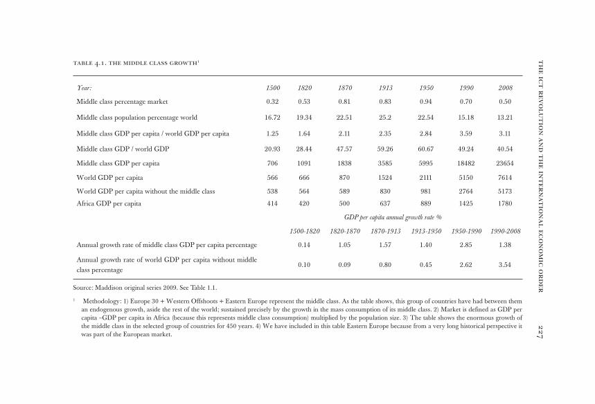
th
e i
ct
rev
olu
tio
n a
nd
th
e i
nt
er
nat
io
na
l e
co
no
mic
or
der
22
7table 4.1. the middle class growth1
Year: 1500 1820 1870 1913 1950 1990 2008
Middle class percentage market 0.32 0.53 0.81 0.83 0.94 0.70 0.50
Middle class population percentage world 16.72 19.34 22.51 25.2 22.54 15.18 13.21
Middle class GDP per capita / world GDP per capita 1.25 1.64 2.11 2.35 2.84 3.59 3.11
Middle class GDP / world GDP 20.93 28.44 47.57 59.26 60.67 49.24 40.54
Middle class GDP per capita 706 1091 1838 3585 5995 18482 23654
World GDP per capita 566 666 870 1524 2111 5150 7614
World GDP per capita without the middle class 538 564 589 830 981 2764 5173
Africa GDP per capita 414 420 500 637 889 1425 1780
GDP per capita annual growth rate %
1500-1820 1820-1870 1870-1913 1913-1950 1950-1990 1990-2008
Annual growth rate of middle class GDP per capita percentage 0.14 1.05 1.57 1.40 2.85 1.38
Annual growth rate of world GDP per capita without middle class percentage
0.10 0.09 0.80 0.45 2.62 3.54
Source: Maddison original series 2009. See Table 1.1.
1 Methodology: 1) Europe 30 + Western Offshoots + Eastern Europe represent the middle class. As the table shows, this group of countries have had between them an endogenous growth, aside the rest of the world; sustained precisely by the growth in the mass consumption of its middle class. 2) Market is defined as GDP per capita –GDP per capita in Africa (because this represents middle class consumption) multiplied by the population size. 3) The table shows the enormous growth of the middle class in the selected group of countries for 450 years. 4) We have included in this table Eastern Europe because from a very long historical perspective it was part of the European market.
carlos obregón228
The failed story of liberalism, however, will not become a success story just by replacing liberalism with nationalism. Nationalism, as we mentioned, failed recently in Argentina and Brazil. And at the global level, nationalism had its days of triumph that ended up in the First World War, the hyper-inflation of the 20s, the Great Economic Depression of the 30s, the surge of Fascism and of a nationalistic communism, the Second World War, and the huge failures of nationalistic communism in the USSR, Mao’s China, and Cuba. If liberalism has been bad, nationalism has been worse.
The world has never had a true international economic order, only few of the potential goals of such an order had been historically addressed. National interests have always prevailed over worldwide considerations. The ICT revolution, however, has brought the world together as never before and it has increased substantially the cost of not addressing prop-erly the global venues for worldwide improvement.
There had been three international economic regimes in the last two centuries. The Gold Standard, Bretton Woods, and the actual neoclas-sical revival with floating exchange rates and free capital flows. In the Gold Standard, the main idea was to control inflation due to previous irresponsible government spending. Gold, due to its restricted supply, was thought that could provide an anchor to global prices and allowed financial and commercial transactions to happen with a degree of cer-tainty —as to the negotiated prices. Beyond that, the functioning of the global economy was left to the markets. However, in its best years, the Gold Standard was closely supervised by the Central Bank of England.
Bretton Woods was the explicit acknowledge that, for the markets to work properly, they need an adequate institutional arrangement. The UN, the IMF, The World Bank, The General Agreement on Tariffs and Trade [GATT, which would later on become the World Trade Organization (WTO)] and NATO were created under this vision. The success of Bret-ton Woods was seen in the rapid reconstruction of Europe as well as in Japan’s westernization and rapid economic growth. However, later on, this same success was going to produce the dismantling of the institutional ar-rangement which was erroneously judge as no longer needed. The IMF and the World Bank changed from institutions oriented towards Europe’s recovery and its proper financial management to its actual role —mainly related to developing economies. But in this process, their goals had also changed, they were no longer concerned with economic development but, mainly, with economic stability and very concrete and minor development goals. The vision has changed from the previous one —that markets, to

the ict revolution and the international economic order 229
work properly, need an institutional arrangement—, to the actual neoclas-sical one —that markets work well if left by themselves. The neoclassical revival was the response to the demise of the Bretton Woods system in 1971 due to the incapacity of the USA to maintain gold convertibility. In this new conception, countries’ autonomous monetary policy is maintained. Oth-erwise, Bretton Woods is turned upside down: instead of fixed exchange rates, floating rates; and instead of capital controls, free capital flows.
The actual system in the grand scheme of things, consequence of the neoclassical revival, was conceived up to 2008 as follows:
1. Markets operate well by themselves (Neoclassical School). 2. The Great Depression was a policy mistake, but we have
learned. It will not happen again. (Lucas). 3. The developed countries do not need the support of global
institutions; they maintain themselves close to equilibrium (Ra-tional Expectations).
4. Developing countries do not develop because they have the improper institutional arrangement, three versions:
a) Washington consensus: they need free prices, open borders, and reduced governments. b) North: they need institutions like the West’s, which allows individual creativity. c) Sen: if mini-mum capacities are guaranteed, development will occur.
5. A world made of national democracies will be peaceful and will have economic progress due to markets’ efficiency and in-dividual creativity.
The actual system, however, was unable to: 1. Provide financial stability to the developed world —we had the
2008 crisis. 2. Provide financial stability to the developing economies. The
floating exchange rates resulted to be too volatile in develop-ing economies and were incompatible with commercial trans-actions; therefore, developing countries had to recur to semi-fixed or fixed exchange rates that were subject of speculation from the free capital flows. The Latin America financial crisis in the 80s, and particularly the Asian financial crisis of the 90s, convinced the developing countries that they needed to protect themselves —in the absence of a proper global institutional ar-rangement— by building huge monetary reserves.
3. Foster development in underdeveloped countries. The coun-tries that followed the neoclassical recommendations did not

carlos obregón230
develop, and the ones that did develop followed a nationalistic development model oriented towards exports to the developed countries: The Asian Development Model.
4. Eradicate poverty. It went down mostly because of the ICT revolution and the Asian Development Model.
In today’s world, criminal activities of all sorts have been globalized: drug and human trafficking, corruption, and so on. Even terrorism has globalized itself. Fiscal paradises have grown significantly; as a result, there is a free movement of financial flows —with inadequate control by the national states—, which means:
a) Governments are losing capacity to implement aggressive fiscal policies because, if they increase taxes to capital too much, it goes away to other locations —through the fiscal paradises.
b) Governments are also losing their supervising capability of corrupt activities because the financial flows cannot be prop-erly followed.
c) The world cannot control the financial flows of criminal or terrorism activities, which makes much more difficult to stop them and to get hold of their illegal wealth.
The ICT revolution has brought the world together and has made evident that the market, without a proper institutional arrangement, does not work properly. The 2008 crisis has provoked a revival of nationalism, protectionism and anti-migration sentiments and policies that are a treat for the future well-being of the global community. It is time to think out of the box and propose modifications to the actual international economic order.
To do that, we need to start by recognizing that:1. There has never been a true international economic order, nor
there will be one in the near future, because national interests dominate the world.
2. Any proposal has to confront the previous fact. 3. The ICT is a technological revolution that has a dynamics
of its own, it cannot and should not be stopped. It can bring enormous progress to the human race if faced properly by an adequate institutional arrangement. Attempts to stop it will fail, although such pretensions can derail the process and become very expensive for humanity.
4. The ICT revolution allows the globalization of many types of activities, criminal ones and terrorism among them. To be
the ict revolution and the international economic order 231
able to control these properly, an institutional arrangement that supervise closely fiscal paradises and financial flows has to be built.
5. That means that the legal global institutional arrangement has to be scaled up.
6. The ICT revolution will increase global trade, and the WTO has to be strengthened. Multilateral agreements are the best way to go. However, given the predominance of national in-terests, regional trade agreements will subsist.
7. National interests always mean the possibility of armed con-frontations, the risk of this can be diminished by recourse to international economic agreements and institutional global ar-rangements.
8. Economic development as a goal has never been properly ad-dressed; it is time to do it.
9. Monetary and financial stability is not guaranteed by today’s regime; improvements should be made.
This chapter will discuss the possibilities to modify the actual inter-national economic order. We start by discussing in the first section the historical background, comparing the actual international economic order to its most recent antecessors, the Gold Standard and Bretton Woods. We will review how each one of these regimes work, and what we have learned from them. In the second section, we list the potential goals that a future international economic order should address, and we review the three previously mentioned regimes against them. We show that the three regimes had been Nash-Pareto inefficient solutions. That is, they are the result of games played between national interests in which each nation optimizes its own position at the expense of sac-rificing the global gains that could have been obtained. In particular, there are many pareto moves —a pareto move is one that benefits at least one of the countries involved without damaging any other country— that have not occurred because the institutional arrangement of the three previously mentioned regimes is inadequate, and therefore do not allow for them to happen. It is shown that Bretton Woods was a step in the right direction, but despite its many contributions, it was still not enough. The actual system has been a step backwards from Breton Woods; this is one of the reasons for the calamities the world economic order has seen, such as the 2008 crisis.
carlos obregón232
In the second section, in the light of the ICT revolution, we pres-ent the potential goals of a future international economic order; and we discuss how each one of them relates to the three “partial” international economic orders regimes previously discussed. The rest of the sections in this chapter are used to discuss the goals listed in section two.
Section three discusses trade, economic growth, and migration. Sec-tion four, monetary and financial stability. Section five, poverty, human development, income distribution, and economic development. Section six briefly discusses the international legal framework and fiscal paradises supervision as a means to control financial flows. Required instruments to reduce tax evasion, and to properly fight terrorism and criminal ac-tivities in general. Section seven succinctly addresses global sustainability and the possibility of a global demographic policy.
The only way for the global economy to operate well is with an ad-equate institutional arrangement —like the Bretton Woods’ success story has shown us. But Bretton Woods is gone, liberalism has failed, and nationalism is resurging; we must not allow it to happen, it will be a great tragedy for humanity. We must —we need to— propose a new interna-tional economic and social order. This is the goal of this chapter, in the understanding, of course, that this is only one of the many proposals that had, and should continue, to be offered. It is not our intention to argue that the proposals offered here are the best ones —that is to be judged by others. Our only goal is to contribute to the discussion and to that purpose, together with our proposals, we will occasionally also review and judge other’s. We hope the reader finds the context of the discussion useful for his own reflections on the topic.
The new international economic order proposed in this chapter goes well beyond the actual system, and it has the main mission of allowing the ICT revolution to bring to the world the huge productivity increas-es that it can offer. If properly managed, in the adequate institutional arrangement, the ICT revolution has the possibility of causing signifi-cant long-term sustainable benefits in economic growth and economic human well-being.
Unfortunately, it is likely that the world will not follow the right path due to entrenched national interest, that will make very difficult to estab-lish the needed international coordination. Therefore, in the next chap-ter we will discuss what policies should the countries follow, assuming the actual institutional framework and the minor adjustments that it will most likely have.

the ict revolution and the international economic order 233
the historical background: what have we learned?
The Gold Standard governed most of the nineteenth century until The Great Depression, it had its best performance from 1880 to 1914, when it what was called The Classic Gold Standard. In this period, most internation-al trade was financed by short-term loans issued in the London market and the long-term projects of underdeveloped countries were financed through loans from private investors —which were obtained in the major financial centers of London and Paris.
The good performance of the Gold Standard was due to the worldwide leadership of the English Central Bank. But this arrangement was only pos-sible thanks to the real economic and political leadership, that England had at that time. World War I interrupted the Gold Standard, the English lead-ership was questioned, and the economic and political agreements that un-derlaid its good functioning dissolved. The return to the Gold Standard in the postwar era was a failure because, by this time, England had lost its pre-vious hegemonic leadership. Finally, the Gold Standard was discontinued in 1931 when other countries demanded from England gold in kind. Note the parallelism: both the Gold Standard and Bretton Woods performed well while there was solid leadership —in the first case of England, in the second of the United States; both were shipwrecked when this leadership was ques-tioned and the leading country was requested to provide gold in kind110.
In reality, large trading monetary-financial systems never worked as independent, autonomous systems —they were always managed— and their good administration required cooperation between the major coun-tries involved. As we said, the Gold Standard in its good time was ad-ministered through the short-term loans of the English market and the interventions of the Central Bank of England. Bretton Woods was ad-ministered by international agencies under the American leadership. The actual system of floating exchange rates that was supposed to be defined freely by the markets; in practice, it has also been managed. The actual system has required broad agreements and negotiations between coun-tries, which involved not only trade, monetary and financial aspects but also different models of economic growth; which recognized and repro-duced distinct relative positions of power at the international level.
110 In both cases the events were related to high internal inflation in the leading country. In the case of England, war’s inflation made the intended return to the previous pound-gold parity a chimera. In the case of the United States, the high inflation was consequence of its expansionary monetary policy.
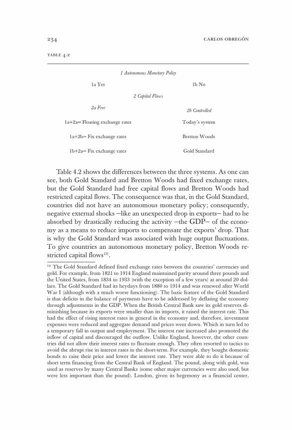
carlos obregón234
table 4.2
1 Autonomous Monetary Policy
1a Yes 1b No
2 Capital Flows
2a Free2b Controlled
1a+2a= Floating exchange rates Today’s system
1a+2b= Fix exchange rates Bretton Woods
1b+2a= Fix exchange rates Gold Standard
Table 4.2 shows the differences between the three systems. As one can see, both Gold Standard and Bretton Woods had fixed exchange rates, but the Gold Standard had free capital flows and Bretton Woods had restricted capital flows. The consequence was that, in the Gold Standard, countries did not have an autonomous monetary policy; consequently, negative external shocks —like an unexpected drop in exports— had to be absorbed by drastically reducing the activity —the GDP— of the econo-my as a means to reduce imports to compensate the exports’ drop. That is why the Gold Standard was associated with huge output fluctuations. To give countries an autonomous monetary policy, Bretton Woods re-stricted capital flows111. 111 The Gold Standard defined fixed exchange rates between the countries’ currencies and gold. For example, from 1821 to 1914 England maintained parity around three pounds and the United States, from 1834 to 1933 (with the exception of a few years) at around 20 dol-lars. The Gold Standard had its heydays from 1880 to 1914 and was renewed after World War I (although with a much worse functioning). The basic feature of the Gold Standard is that deficits in the balance of payments have to be addressed by deflating the economy through adjustments in the GDP. When the British Central Bank saw its gold reserves di-minishing because its exports were smaller than its imports, it raised the interest rate. This had the effect of rising interest rates in general in the economy and, therefore, investment expenses were reduced and aggregate demand and prices went down. Which in turn led to a temporary fall in output and employment. The interest rate increased also promoted the inflow of capital and discouraged the outflow. Unlike England, however, the other coun-tries did not allow their interest rates to fluctuate enough. They often resorted to tactics to avoid the abrupt rise in interest rates in the short-term. For example, they bought domestic bonds to raise their price and lower the interest rate. They were able to do it because of short term financing from the Central Bank of England. The pound, along with gold, was used as reserves by many Central Banks (some other major currencies were also used, but were less important than the pound). London, given its hegemony as a financial center,
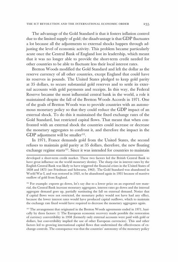
the ict revolution and the international economic order 235
The advantage of the Gold Standard is that it fosters inflation control due to the limited supply of gold; the disadvantage is that GDP fluctuates a lot because all the adjustments to external shocks happen through ad-justing the level of economic activity. This problem became particularly acute once the Central Bank of England lost its leadership, which meant that it was no longer able to provide the short-term credit needed for other countries to be able to fluctuate less their local interest rates.
Bretton Woods modified the Gold Standard and left the dollar as the reserve currency of all other countries, except England that could have its reserves in pounds. The United States pledged to keep gold parity at 35 dollars, to secure substantial gold reserves and to settle its exter-nal accounts with gold payments and receipts. In this way, the Federal Reserve became the most influential central bank in the world, a role it maintained despite the fall of the Bretton Woods Accords in 1971. One of the goals of Bretton Woods was to provide countries with an autono-mous monetary policy so that they could reduce the GDP impact of an external shock. To do this it maintained the fixed exchange rates of the Gold Standard, but restricted capital flows. That meant that when con-fronted with an external shock the countries could increase or decrease the monetary aggregates to confront it, and therefore the impact in the GDP adjustment will be smaller112.
In 1971, France demands gold from the United States, the second refuses to maintain gold parity at 35 dollars, therefore, the new floating exchange regime starts113. Since it was intended for countries to maintain
developed a short-term credit market. These two factors led the British Central Bank to have great influence on the world monetary destiny. The sharp rise in interest rates by the English Central Bank was likely to have triggered the financial crises in the United States of 1838 and 1873 (see Friedman and Schwartz, 1963). The Gold Standard was abandoned in World War I, and was restored in 1925, to be abandoned again in 1931 because of massive outflow of gold from England.
112 For example: exports go down, let’s say due to a lower price on an exported raw mate-rial, the Central Bank increase monetary aggregates, interest rates go down and the internal aggregate demand goes up, partially sustituting the fall on external demand. Notice that if capital flows were not restricted, the monetary policy would not have had any effect, because the lower interest rates would have produced capital outflows, which to maintain the exchange rate fixed would have required to decrease the monetary aggregates again.
113 The arrangement that originated in the Bretton Woods agreements ended in 1971, basi-cally by three factors: 1) The European economic recovery made possible the restoration of currency convertibility in 1958 (formerly only external accounts were paid with gold or dollars, but convertibility implied the use of other European currencies). This and other factors led to growing international capital flows that undermined the effectiveness of ex-change controls. The consequence was that the countries’ autonomy of the monetary policy
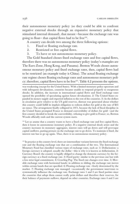
carlos obregón236
their autonomous monetary policy (so they could be able to confront negative external shocks through an expansive monetary policy that stimulated internal demand), that meant —because the exchange rate was going to float— that capital flows had to be free114.
A country can decide two among the three following options:1. Fixed or floating exchange rate. 2. Restricted or free capital flows.3. To have or not autonomous monetary policy.The Gold Standard choses fixed exchange rates and free capital flows,
therefore there was no autonomous monetary policy (today’s examples are The Euro Zone, Hong Kong, and Panama). Bretton Woods choses auton-omous monetary policy and fixed exchange rates, then, capital flows had to be restricted (an example today is China). The actual floating exchange rate regime choses floating exchange rates and autonomous monetary poli-cy; therefore, capital flows have to be free115. Table 4.2 presents the options.
was weakening (except for the United States). With a limited monetary policy spectrum and with infrequent devaluations, countries became unable to respond properly to exogenous shocks. In addition, the increase in international capital flows and fixed exchange rates opened the possibility of speculating against future devaluations. 2) The United States ex-panded its money supply and exported inflation to the rest of the countries. 3) As the dollars in circulation grew relative to the US gold reserves, distrust was generated about whether this country could fulfill its implicit obligation to redeem dollars for gold at the rate of $35 an ounce. The arrangement finally collapsed in 1971, because the lack of fiscal discipline in the United States prompted France to demand convertibility of dollars for gold —and the first country decided to break the convertibility, refusing to give gold to France; so, Bretton Woods officially ends and the current system starts.
114 Let us asume that a country wants to have a fixed exchange rate and free capital flows, then it losses its autonomous monetary policy. If a negative external shock arises and the country increases its monetary aggregates, interest rates will go down and will provoque capital outflows, putting presure on the exchange rate to go down. To maintain it fixed, the interest rate has to go up again. Thus, there is no autonomous monetary policy.
115 In practice at the country level, there are intermediate variants between the fixed exchange rate and the floating exchange rate that are a combination of the two. The International Monetary Fund has classified various types of exchange rates, such as: 1) Dollarization: a foreign currency is adopted, usually the dollar —this is why it is known as dollarization. 2) Currency Board: the country is legally obliged to change the domestic currency by the for-eign currency at a fixed exchange rate. 3) Fixed parity: similar to the previous one but with a less strict legal commitment. 4) Crawling Peg: The fixed rate changes over time. 5) Mov-able exchange rates with horizontal bands: in addition to sliding, the exchange rate moves within certain bands that are specified. 6) Floating exchange rate —freely determined by the market. 7) Floating exchange rate managed —occasionally the government intervenes to systematically influence the exchange rate. Exchange rates 1 and 2 are fixed parities since the countries that adopt them cannot really print dollars and therefore their reserves, for their balance of payments ouflows, depend on other countries. Exchange rates 4 and 5 are
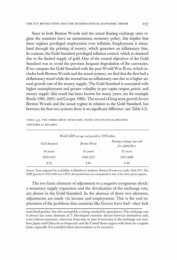
the ict revolution and the international economic order 237
Since in both Bretton Woods and the actual floating exchange rates re-gime the countries have an autonomous monetary policy, this implies that these regimes privileged employment over inflation. Employment is stimu-lated through the printing of money, which generates an inflationary bias. In contrast, the Gold Standard privileged inflation control, which is obtained due to the limited supply of gold. One of the central objectives of the Gold Standard was to avoid the previous frequent degradation of the currencies. If we compare the Gold Standard with the post World War II era (which in-cludes both Bretton Woods and the actual system), we find that the first had a deflationary trend while the second has an inflationary one due to a higher an-nual growth rate of the money supply. The Gold Standard is associated with higher unemployment and greater volatility in per capita output, prices, and money supply (this result has been known for many years, see for example Bordo 1981, 2001; and Cooper 1982). The record of long-term growth favors Bretton Woods and the actual regime in relation to the Gold Standard, but between the first two systems there is no significant difference (see Table 4.3).
table 4.3. the three great monetary, trade and financial regimes
(historical record)
World´s GDP average real growth in 1990 dollars
Gold Standard Bretton WoodsFloating exchange rates and
free capital flows
43 years 31 years 37 years
1870-1913 1940-1971 1971-2008
2.12 3.81 3.49
Source: Years adjusted for availability in Maddison’s database. Bretton Woods was really 1944-1971. The GDP growth in 1913-1940 was 1.87%, this period does not correspond to any of the three great regimes.
The two basic elements of adjustment to a negative exogenous shock: a monetary supply expansion and the devaluation of the exchange rate, are absent in the Gold Standard. In the absence of these two elements, adjustments are made via income and employment. This is the real ex-planation of the problems that countries like Greece have had —they lack
semi-fixed parities, but also susceptible to being attacked by speculators. The exchange rate 6 always has some elements of 7. Developed countries discuss between themselves and, even without announce, intervene from time to time if necessary in the exchange rate mar-kets. Japan and China do so frequently and the United States argues with them on a regular basis, especially if it considers these interventions to be excessive.
carlos obregón238
the possibility of a devaluation and do not have a monetary policy of their own. Therefore: imports have to fall via a reduction in national income generating large unemployment; and promoting exports requires substantial declines in nominal wages that are downright unpopular.
As already noted, both Bretton Woods and the actual regime, allow countries to have an autonomous monetary policy, but they differ in that Bretton Woods has fixed exchange rates and capital controls, while the actual system has free capital flows and floating exchange rates. Bret-ton Woods allows the devaluation adjustment, but only occasionally and with the help of international institutions. The International Monetary Fund was created initially with this objective in mind (even though it modified its objectives later on). The advantage of the actual system is that the floating exchange rate allows an adjustment to an exogenous shock via the price of the currency.
If, as exemplified, exports fall, this implies that the demand for the local currency falls and then its price falls in relation to other currencies. The new lower exchange rate stimulates exports again and discourages imports. The fluctuation in the exchange rate reduces fluctuations in employment and income resulting from real external shocks in the balance of payments. This is the main advantage of the actual system over Bretton Woods. The actual regime has three additional advantages: it produces efficiency in cap-ital flows, avoids the problems associated with exchange rate controls and it does not present the asymmetry that existed in Bretton Woods between the dollar as reserve currency and the other currencies.
However, the actual regime also has two main drawbacks. The first is that, due to fluctuations in the price of the currency, uncertainty is pro-duced as to the level of exchange rate in commercial transactions. Exces-sive fluctuations make international trade operations very difficult. The second disadvantage is that the free flow of capital favors financial instabil-ity (see Table 4.4). The first disadvantage had the consequence that floating exchange rates were replaced in many of the underdeveloped countries by fixed or semi-fixed exchange rates. The contradiction between free capital flows and the semi-fixed or fixed exchange rates in the underdeveloped countries led to a greater frequency of financial crises in these countries116.
116 There is a clear relationship between the world trade, monetary and financial regimes, and financial crises in developing countries. The 1971-dollar’s crisis was a major antecedent of the financial crises in underdeveloped countries in the 1980s and the 90s. The dollar’s crisis produced the oil price increase in the 70s —because the oil producers were selling in dollars and were buying from Europe in other currencies, therefore they had to increase the dollar price of oil. The oil shock was wrongly received with accommodative policies by

the ict revolution and the international economic order 239
The outcome has been the recent trend to very high reserves in these coun-tries. The advantages and disadvantages of the three systems are presented in Table 4.4.
table 4.4. advantages and disadvantages of the three great regimes
(priority given to each goal)
Gold Standard Bretton Woods Today’s system
Inflation control high low low
Full employment low high high
Defending employment against external shocks
low medium high
Certainty of commercial prices high high low
Efficient allocation of resources high low high
Financial stability low high low
Source by author.
Each one of the three regimes mentioned respond to the specific needs of its historical epoch. The Gold Standard emphasized the control of in-flation due to the frequent degradations of the currency in previous times. Bretton Woods privileged employment because the antecedent was The Great Depression. The present system arose because the asymmetry be-tween the reserve currency and the other currencies became unaccept-able —once the European and Japanese economic recovery took place.
the developed economies —producing the 70s inflation, which ended with Volcker highly restrictive monetary policy and the rapid rise of interest rates to unimaginable levels. The high interest rates were the major reason of the financial crisis in developing countries in the 80s —mainly in Latin America. Because the floating exchange rates of the underdeveloped countries were too volatile against the hard currencies of developed countries, the under-developed countries opted for semi-fixed and fixed exchange rates. But this made them vulnerable to financial speculation. The current system showed one of its great weaknesses: on one hand, the volatility of exchange rates is excessive, on the other; the semi-fixed or fixed exchange rates are easy prey to speculation. In the 90s, the Asian crisis, because of speculative reasons, involved countries with solid economic basis. The lesson learned is that the underdeveloped countries had to protect themselves against speculative attacks. This is why they have recently opted for large international reserves.
carlos obregón240
What have we learned? The Gold Standard taught us that an interna-tional economic order requires the decisive leadership of the most power-ful country (or countries). We also learned that adjustments to external shocks through GDP were extremely expensive; therefore, an autono-mous monetary policy at the country level is necessary. At the global level, both Bretton Woods and the actual system learned this lesson, but as strange that it may seem, the Euro Zone has returned to an arrange-ment in which countries do not have an autonomous monetary policy —a position which theoretically does not make much sense. We will later on argue that the Euro Zone has to implement a different arrangement.
Bretton Woods taught us that a proper institutional arrangement can be very effective in promoting both economic growth and financial sta-bility. The actual floating exchange rate regime has taught us that free capital flows, together with the ICT revolution, globalized finances to the point where the national regulators could not understand what was going on any longer. Therefore, there is a need for the national regulators to be much closer to the markets, and to get together with regulators from oth-er countries to understand the world’s financial market. It also taught us that the exchange rate volatility was too high for developing economies and that, as theoretically expected, semi-fixed or fixed exchange rates were not the solution because of two reasons: 1) they left the country without a proper autonomous monetary policy; and 2) they estimulate capital flows speculation that generates financial crisis.
the potential goals of the international economic order
In what follows we present the potential goals of a future international economic order; and we discuss how each one of them relates to the three “partial” international economic orders regimes previously discussed.
1. To promote and sustain world’s economic growth. Economic growth was seen as a natural outcome of allowing the markets to freely operate by themselves. Only Bretton Woods saw the need to have it as a specific institutional international goal.
2. Establish a legal international framework for national and other disputes to be solved. It was a concern in the three re-gimes, but only Bretton Woods saw the need to go beyond the
the ict revolution and the international economic order 241
minimum requirements. This goal has always been opposed by the national interests of the leading countries who see their own national legal system as reference for the world.
3. Organize global trade. A concern due to Bretton Woods, which has been able to survive.
4. Provide monetary and financial stability. In the Gold Stan-dard, it supposes to be a natural consequence of using gold as the standard. In the actual system, it was conceived as a natural consequence of implementing free capital flows and floating exchange rates. Only Bretton Woods recognizes the need to implement a specific institutional arrangement.
5. Promote economic development. It supposes to happen natu-rally both in the Gold Standard and in the actual regime. It is not a concern in Bretton Woods, which was mainly focused in the recovery of Europe and Japan.
6. Promote human development. It is mainly a concern in the actual system, but refers only to minimum welfare standards.
7. Eliminate global poverty. It is mainly a concern in the actual system, but refers only to extreme poverty.
8. Give a solution for migration. It has always been discussed, but it has never been a major concern in any of the three re-gimes.
9. Eliminate or supervise the fiscal paradises very closely. It has always been discussed but it has never been a major con-cern in any of the three regimes.
10. Promote national control of taxes for which 9 is useful. It has always been discussed, but never has been taking seriously by any of the three regimes.
11. Fight global crime and global terrorism, for which 9 is also useful. It has always been discussed, but never has been taking seriously by any of the three regimes.
12. Global sustainability —environment. Discussed seriously only in the actual regime, but still very controversial, since it damages powerful national interests.
13. A global demographic policy. Not a concern for any of the three regimes. It has always been assumed that this is a prob-lem to be solved at the national level.
Why have so few international potential goals been addressed histori-cally? The answer is very simple, because the global problems are not
carlos obregón242
any country’s specific concern —each country looks for its own interest, and it is only concerned with worldwide problems as far as they relate to its own national interest. Using game theory, the world is in a Nash equilibrium, which is without doubt pareto suboptimal. It is clear that there are many potential moves that will benefit everybody, but they do not happen because the path to get there is not without the risk that some-one would end worse off. Take goal 5) as an example. It is clear that an economic plan to promote the economic development of underdeveloped countries will benefit everybody, just like the Plan Marshall did after the WWII. But developed countries do not want to pursue this route because there is always the risk that one developed country puts more of the cost and take less of the benefit, ending up being a loser. Creating the proper institutional framework to guarantee that only pareto moves will be taken by all the participants has been proven to be very difficult in a world in which national interest predominates.
Today’s problem, however, is that the actual regulatory global system has become extremely inefficient because of the challenges brought about by the ICT revolution. Technology has drastically changed the world, by bringing countries closer to each other; consequently, the solutions based only in national interests have become extremely inefficient —as the 2008 crisis and global criminal activities and terrorism have shown.
Trade, economic growth and migration
As we have seen in chapter one, the ICT revolution has increased global economic growth; thus, even with the 2008 crisis the world continues grow-ing at high rate (Table 1.1). Trade has also increased significantly: world’s exports as a percentage of GDP went from 15.7% average in 1966-1990 to 26.1% in 1991-2016 (Table 1.23). Foreign direct investment flows are very high for historical standards (Table 1.4), and has gone mainly to China (Table 1.5). Foreign technology, high savings and exports to the developed world have made China’s growth very fast: an annual rate of 9.0% between 1990 and 2016 (Table 1.21). China went from 1871, 2011 PPP dollars, GDP per capita in 1990 (36% or World’s average) to 14401 in 2016 (96% of World’s average, Table 1.22a, to be found in annex at the end of the book). China’s merchandise exports share of total world merchandise exports went from 1.8% in 1990 to 13.2% in 2016. China plus Hong Kong share was in 2016
the ict revolution and the international economic order 243
16.39%, significantly higher than that of USA, Canada, and Mexico together —13.91%— or Germany’s share, France, and the UK together —14.11%— Ta-ble 1.8. The increase in China’s exports happened with two additional factors to consider: 1) China’s share of manufacture exports to merchandise exports was the highest in the world, 94.3% (Table 1.10); and 2) China maintained a high share of merchandise exports to developed countries (Table 1.14).
Thus, China has dramatically changed due to the ICT revolution and the adoption of the Asian Development Model, and it has changed the world. Any analysis of where the world is today and any prospective discussion as to where it is going to be, necessarily has to be related to the ICT revolution and to China. It is important to distinguish the two clearly. The ICT revolution will continue with no doubt, however, most certainly, it will encounter some difficulties due to protectionist policies. Technology will prevail at the end, as it always does, but if the protection-ist measures are temporarily successful, they may slow down the ICT revolution’s advances. China will continue to be a key player, but it has difficulties of its own, such as its political future and how well will it cope with becoming a middle-income country. Therefore, we do not know to what extent in the future the ICT revolution will involve significantly oth-er key countries or not, but there are already large populated Asian coun-tries that are good candidates to start replacing China, at least partially.
What is certain is that the ICT revolution has already changed the world. Many indicators, like the global income distribution or the pov-erty level, have improved but we must be aware that it is mostly due to China. Take the case of the global income distribution; it clearly has improved (Table 2.8). But if we take away China and India, the rest of the world from 1980-2008 or 1990-2016 does not converge to the West GDP per capita (Tables 2.6 and 2.26).
Democracy has strengthened the political power of the middle class in the developed economies, which can be shown in an increase in its share of disposable income in the twentieth century (Table 2.14), mainly due to government expenditures and social expenditures’ rapid increase as a percentage of GDP (Table 2.13). Thus, while national democracies in the developed world have consolidated national governance, at the world level governance has weakened —at least in relationship to Bretton Woods. The ICT revolution has fostered rapid globalization and the conflict of global capitalism and consolidated national democracies in the developed countries has become more acute, that is why protectionism, however, and nationalism are revival tendencies in these countries.
carlos obregón244
The ICT revolution has substantially improved the world in which we live, but it has not done so evenly: there have been big winners, losers, and non-participants. Therefore, in terms of averages: economic growth is higher, the global income distribution is better and poverty is substantially less; but that obscures the fact that there have been losers and non-participants.
The most important threat for the future comes from the losers in the developed economies that, together with traditionally right wing nation-alistic groups, are voting for protectionist measures, for anti-migration policies and for a nationalistic perspective. This will not only not work but can create chaos and global disarray; as it happened before, when nationalism triumphed.
The ICT revolution means that global trade and economic growth will continue to have an upward trend in the future, but the world’s outlook will be the better if the global institutional arrangement is the adequate one. Protectionism is a real threat.
As for migration: the ICT revolution has made migration unneeded, as we discussed in chapter one. Firms are better off moving manufacturing produc-tion offshore instead of bringing migrants. Therefore, migration will continue growing as decreasing transportation costs will make it easier and as the de-mography from the developed countries requires it (because their populations are getting old), but it will not be in the center of future productivity revolu-tions. Multilateral agreements related to migration issues are very unlikely.
What institutional global policies are required? The WTO organiza-tion should be strengthened, multilateral agreements should be preferred to regional or bilateral ones, and protectionism should be avoided. Trade is not the place to resolve unemployment or income distribution prob-lems; these have to be addressed with specific policies at the national level that will be discussed in chapter five. The world must be allowed to rip the benefits that the ICT revolution can provide.
The ICT revolution does not hurt the developed countries; it benefits them in several ways. The higher productivity translates into:
1. Lower expected inflation.2. Lower real long interest rates —due to higher global savings. 3. 1 and 2 mean lower nominal long interest rates and more cred-
it availability, which substantially increase the population’s standard of living in developed countries.
4. Lower prices today, which also benefit the living standard of the population in developed countries.
the ict revolution and the international economic order 245
The benefits clearly offset the costs of income redistributions and greater unemployment in some sectors of the developed economies. The costs should be addressed with specific national policies, but trade should not be reduced because its benefits clearly outweigh its costs by much.
A lot of confusion has been created by blaming the 2008 crisis in trade unbalances and over saving, but as we have shown in the previous chapter, that explanation was wrong. Hence, there is no need to balance trade. Bal-ancing trade means drastically reducing the possibility set of global potential trade arrangements, which necessarily has the consequences of diminishing the amount of global trade. In very specific terms, the proposal of balancing global trade amounts to reducing USA’s trade deficit and the surplus of the main exporting countries. But is there anything wrong with a large USA trade deficit? The answer is that there is nothing wrong. In general, the main problem of a large trade deficit is the potential future problem of not being able to finance it. The USA, however, does not have this problem. The dol-lar has been the global currency reserve per excellence. The USA is the only real military power left. In fact, other countries had been very happy to save and increase dollar reserves because they have been able to develop this way.
The world before the 2008 crisis had successfully discovered that eco-nomic development does not occur when rich countries export capital to poor countries, but the other way around. It is their own savings what develop the poor countries; because of the well-known duality, savings are also exports. It is by exporting to the middle class of the developed countries —mainly the USA— that some countries in Asia have devel-oped. This, by the way, is the only case in the history of capitalism that underdeveloped countries did develop. For the USA it had meant enjoy-ing huge global productivity increases due to the incorporation of large populations at low wages —that substantially improved the American people’s way of life. There was nothing wrong with the world before the crisis, we should not be afraid to go back to that status quo.
Monetary and financial stability
There are critical problems to solve related to monetary and financial stability. The most important ones are:
1. Global regulation of financial markets, mainly in the devel-oped world.

carlos obregón246
2. Define the role of monetary policy versus fiscal policy.3. Solve the problem of the excess volatility of exchange rates,
mainly in developing countries, to prevent the enormous costs associated with speculative capital flows.
4. Restructure the monetary and financial system of the Euro Zone to allow countries in extreme situations to have a mon-etary policy of their own.
5. Redefine the role of the IMF.6. Define the global monetary and financial arrangement that will
be able to deal with the previous listed problems.To start, we should identify two main causes of the previously men-
tioned problems: 1) the belief in the capacity of the markets to adjust themselves, and 2) the unwillingness of the developed countries to truly commit to sustain and defend a global monetary and financial arrange-ment. Removing any one of these causes is a titan’s task, and it may turn out to be impossible. But given the huge costs that the world has recently experienced by not having an appropriate institutional arrangement, it is worth at least a discussion. What are the potential alternatives?
Markets only work properly given the right institutional arrangement. Markets can manage probabilistic risk very well, but they are unable to manage future uncertainty (what Mervyn King calls radical uncertainty). The only way to bridge between the now and the future is by establish-ing the proper institutions. What provides the bridge is the credibility of the institutions commitment to maintain stability; this was Knight and Keynes’ central message. What institutions do is provide information, they provide the framework that make private contracts credible and re-spectable, and show the negotiated path to avoid some of the traps of the prisoner’s dilemma, i.e., the difficulty of achieving a good outcome given the obstacles for cooperation. Institutions may be the difference between the “wrong games” and the “good games”; because they may put penal-ties to the participants that do not follow pareto moves —i.e., moves in the direction of a pareto optimum (a point in which none of the participants can benefit without hurting some other participant).
What commitments must regulators, governments, and Central Banks make? The most important one is that they strongly commit to maintain stability. Lately, we have seen many mistakes related to this point; which makes clear that it is not well understood. Two examples are letting Lehman Brothers go bankrupt and not supporting Greece – ie asking private banks to absorb huge losses in Greek’s debt.
the ict revolution and the international economic order 247
The name of the game is not overregulation. Markets must be able to operate freely, but regulators must be vigilant and intervene when need-ed, in early stages —as the USA regulators should have done with the subprime adjustable rate loans market crisis. Regulators have to be very familiar with the diverse types of risk in the banks’ balance sheets and of other financial institutions and players that they suppose to supervise. It is impossible to intervene on time without such understanding, which is exactly what happened in 2008. USA regulators did not understand the risk in the balance sheets of the banks and other financial players associ-ated with the subprime adjustable rate loans market crash, neither did the European regulators.
What is the role of monetary policy?
Before, answering this question would have been easy, the answer could have been found in any good textbook. Today, it is not that easy. Central Banks had intervened in the markets to perform huge buys of private financial assets. The first things to clarify are the following: Did they do it only because of an emergency? Will, or should they continue doing it? What are the implications?
Traditionally, the role of Central Banks was seen as to maintain control on monetary aggregates to prevent governments from overspending. This is reflected in a single mandate to the Central Bank to maintain price sta-bility —i.e. reduce the degree of uncertainty associated with the price level over the long run. It was also thought by some that Central Banks should also care about short-term output fluctuations, because these fluctuations could be influenced by monetary policy. That is why some banks, like the Fed, have a dual mandate. Moreover, it was agreed that the Central Bank role goes beyond monetary aggregates, it has to inspire trust. That is why the main Central Banks adopted an inflation targeting policy —for most of them is two percent, which precisely aims at communicating the serious-ness of the commitment and to inspire trust. The two main traditional Cen-tral Bank munitions have been: first, setting the Central Bank rate; second, buying or selling government bonds of different maturities.
But the 2008 crisis raised a new question, should Central Banks also care about big disequilibriums like the 2008 crisis? The answer before 2008 was that they should not; in fact, these kind of disequilibriums
carlos obregón248
were not suppose to have happened. Today the answer is, clearly, yes. However, this implies new tasks for the Central Banks such as guiding the allocation of credit amongst sectors, through control policies usually known as macroprudential.
In 2008, with interest rates of all maturities going close to zero, the traditional Central Bank munitions were exhausted. That is why they went into buying private sector assets, which really meant they were taking credit risk, and entering the realm of fiscal policy. Should they continue?
The answer is yes, it will have several advantages: 1) it will main-tain the Central Banks paying attention to real market conditions; 2) the Central Bank has more flexibility to act than the fiscal policy. It is truly the discovery of a new instrument that is a hybrid between fiscal and monetary policies, and that should continue to be used. But a much well thought legislation and regulation for this activity must be designed.
Global regulation of financial markets, mainly in the developed world
A more active monetary policy necessarily requires global coordination. Giving free capital flows the macroprudential task necessarily implies co-ordination amongst countries. What we learned with the 2008 crisis is that financial risks are globally interconnected. Financial regulation has to be global, this requires building the proper institutions to be able to do so.
The Euro Zone
The Euro Zone was not well designed. An economic zone, to be able to have a unique monetary policy, must also have a unique fiscal policy and free migration. Migration in the Euro Zone is free. The Maastricht Treaty supposedly obliged countries to coordinate their fiscal policy —in the practical world it did not happen. Therefore, as we saw in Tables 3.10 and 3.11, the monetary policy was too accommodating for several coun-tries —because their fiscal policies were not aligned. Germany and France tolerated other countries’ large governmental and merchandise deficits to be able to export to them. The 2008 crisis made evident the disarray already occurring in the Euro Zone.

the ict revolution and the international economic order 249
Once countries like Greece entered the crisis, the weakness of the Euro Zone became evident. The solution for a significant negative external shock like Greece experienced can be one of four:
1. Receive huge capital inflows from other European coun-tries —but the required flows were and are politically unac-ceptable in Germany and in France.
2. Change the rules of the Euro Zone: allowing Greece tem-porarily out —to have its own currency, to establish capital controls, to recover its own monetary policy, and devalue its new currency against the euro establishing a new fixed exchange rate between the new currency and the euro.
3. Change the rules of the Euro Zone: allowing Greece tem-porarily out, to have its own currency and letting it float against the euro, this will bring back monetary autonomy to Greece and soften the impact of the recovery.
4. Maintain the status quo with limited capital inflows to Greece from other European countries, which means a draconian adjustment —through GDP falls to reduce imports, and through reducing nominal wages to promote exports— ex-tremely expensive economically, and —especially— socially for Greece. Notice that this option is very similar to the Gold Standard regime. The fourth option was taken, but it is inferior to the second and the third. We will argue that the third option should have been taken, and that it should have been reflected in a permanent change of rules in the Euro Zone.
It is very simple, if the Euro Zone wants to survive, it has to modify its rules; it cannot ask countries to go through draconian adjustments each time they have a significant external shock. As long as Europe is not one single country, each one of the countries participating is ex-posed in distinct ways to different external shocks —thus not even an agreed fiscal policy (like the Maastricht’s treaty) will solve the issue. Modern economic tools tell us that, when confronted with an external shock, the optimum solution is for the country to have its autonomous monetary policy. Now, as we saw before, to have an autonomous mon-etary policy there are only two options: 1) a fixed exchange rate and capital controls (like Bretton Woods); and 2) a floating exchange rate and free capital flows (like the actual regime).
carlos obregón250
In our opinion, given that the world’s actual regime is the second option (which is the right option, given the flexibility required by the ICT revolution), this is the one that the Euro Zone should use when in especial occasions a country is confronted with a significant external shock. How will it work? In the new proposed regime, there would be multiple currencies, one for each country. In normal times, the ex-change rates between the diverse currencies will be fixed and there will be free capital flows. Therefore, in normal times the new regime will mimic the actual Euro Zone regime. But when a country faces a signifi-cant external shock it will be able to let its currency float, recovering its autonomous monetary policy, which in fact means leaving temporarily, only in monetary terms, the Euro Zone.
The IMF
The International Monetary Fund was originally designed to provide exchange rate and financial stability to contribute to the recovery of Eu-rope; but it has changed and has become a short-term lender for develop-ing countries. As a consequence, the IMF is no longer concerned with economic recovery or growth. The reason is simple, in the beginning, it had full support from the world’s leader —the USA—; today, developed countries put a lot of pressure on the IMF to recover its loans in a short period. To be able to go to its initial role, it would need much more sup-port from the developed countries.
The excess volatility of exchange rates
As we mentioned before, floating exchange rates have resulted too vola-tile in developing countries. Therefore, they adopted fixed or semi-fixed exchange rates, which, under free capital flows, were soon the target of speculators and very serious financial crisis have occurred. To avoid this situation, the developing countries have decided to create very large international reserves that would allow them to control better their ex-change rates. However, the economic cost of doing so is high, and the exchange rates still fluctuate more than it is desired.

the ict revolution and the international economic order 251
A cheaper alternative that will work much better would be to strength-en the IMF and charge it with maintaining exchange rate stability in de-veloping countries. In practice, that means a very strong IMF that has to be fully back up by the developed countries. Does it make sense? It only does if it is linked to an economic development strategy to modernize the underdeveloped countries. See the section below titled: Development, a great global opportunity.
Towards a new global monetary and financial institutional arrangement
The ICT has progress so fast that institutions have not been able to cope with it, even in developed countries. As we showed in the previous chap-ter, USA and European regulators did not understand what was really going on in the financial markets. Therefore, they did not intervene on time and that explains the magnitude of the 2008 financial crisis. One of the reasons is that the ICT revolution has globalized situations that used to be national. At the global level, institutions had traditionally been less developed; and global coordination had been slower and more inefficient than the one we find in a typical developed country. That explains why the European regulators insisted for years that the subprime crisis in the USA was not their concern, they never understood the globalizing power of the ICT revolution.
However, due to the 2008 crisis, today’s monetary policy is already well beyond the boundaries of national monetary aggregates. It has en-tered the realm of credit —credit is a global phenomenon— and, there-fore, worldwide coordination (particularly among the main players, the developed countries) is required. Macroprudential policies cannot be understood or executed without global coordination. Steps in that direc-tion have been taken already, but they are still coordinated, mainly, by the countries themselves. The international institutions are not strong enough; they really do not have an independent role of their own. The future risk is that, as the memory of the 2008 crisis fades away, global coordination amongst countries weakens again. To avoid such risk, the IMF —and other global financial institutions— must become stronger and truly independent.
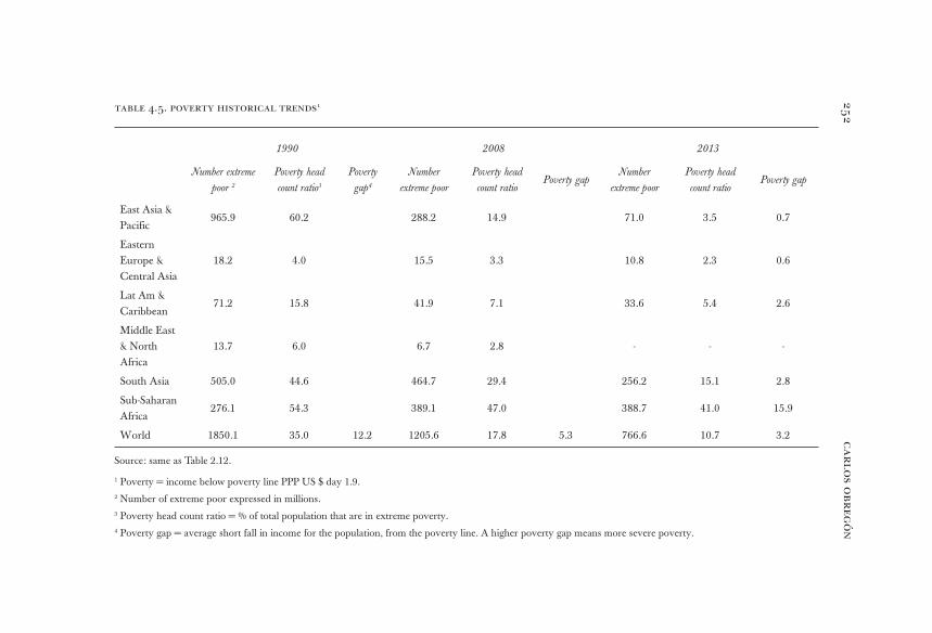
ca
rlo
s o
br
eg
ón
25
2table 4.5. poverty historical trends1
1990 2008 2013
Number extreme
poor 2
Poverty head
count ratio3
Poverty
gap4
Number
extreme poor
Poverty head
count ratioPoverty gap
Number
extreme poor
Poverty head
count ratioPoverty gap
East Asia & Pacific
965.9 60.2 288.2 14.9 71.0 3.5 0.7
Eastern Europe & Central Asia
18.2 4.0 15.5 3.3 10.8 2.3 0.6
Lat Am & Caribbean
71.2 15.8 41.9 7.1 33.6 5.4 2.6
Middle East & North Africa
13.7 6.0 6.7 2.8 - - -
South Asia 505.0 44.6 464.7 29.4 256.2 15.1 2.8
Sub-Saharan Africa
276.1 54.3 389.1 47.0 388.7 41.0 15.9
World 1850.1 35.0 12.2 1205.6 17.8 5.3 766.6 10.7 3.2
Source: same as Table 2.12.
1 Poverty = income below poverty line PPP US $ day 1.9.2 Number of extreme poor expressed in millions.3 Poverty head count ratio = % of total population that are in extreme poverty.4 Poverty gap = average short fall in income for the population, from the poverty line. A higher poverty gap means more severe poverty.
the ict revolution and the international economic order 253
The actual regime of floating exchange rates and free capital flows is needed for the speed of change involved in the ICT revolution. However, it has the risks that, precisely because of the speed at which it can change, it can become disruptive of the economic order —as the 80s Latin Ameri-can financial crisis, the 90s Asian crisis and the 2008 crisis have shown. In order to avoid such disruptive events, the actual regime needs a much stronger global institutional framework. This does not mean overregula-tion, means regulators that do participate in the markets and understand them. Regulators that are supervising the credit flows and the banks’ bal-ance sheets and the ones of other financial institutions and players at the global level. Regulators that are always asking themselves whether the institutional arrangement is or is not providing the institutional certainty related to the future that is required. The speed of financial innovations that the ICT revolution allows requires very fast regulating innovations at the global level —to that account, global financial institutions must be substantially strengthened.
Poverty, human development, income distribution and economic development
Many global indicators present a positive scenario for the future; the global income distribution is improving, the United Nations Human De-velopment Index (HDI) shows a clear upward trend and poverty has been declining rapidly. All these have created several illusions. The first one is that the global program against extreme poverty is a success. The second illusion is that the global program to improve the quality of hu-man life is a success. The third one is that the underdevelopment prob-lem will be solved by itself.
Let us start with the third one. It is true that the global income distribu-tion is improving, and that it is due to the fact that the between country inequality is decreasing. It is true that the underdeveloped countries are converging towards the developed ones. But, it is not true that this will solve the underdevelopment problem. Convergence is relevant because the countries involved are heavily populated; however, it is a very limited phe-nomenon in terms of the countries participating. Moreover, while it is true that the ICT revolution will continue and it may expand to other popu-lated countries in Asia. Even if it happens, it would still be a concentrated phenomenon. There is discussion as to whether the global convergence is
carlos obregón254
due to China only and, some more recent data, seems to indicate that it may include other countries, but they are still a limited number. With all of them related to the Asian Development Model, which given its export-ing characteristics may present difficulties if it were to be applied to most of the underdeveloped countries. However, in any case, that is not a likely scenario. If the ICT expands, it will be to a limited set of countries.
Is the improvement in the global income distribution a relevant phe-nomena? Of course, because it involves large populations. Will it solve the problem of underdevelopment? No, because of its limited character. Moreover, we should not lose sight of the fact that, in terms of the global income distribution, despite its relative recent improvement, the world is a very unjust place. Any way we measure it, it is less equal than the most unequal countries on earth. The truth is that the world today is very inegalitarian; the citizenship rent, as defined in chapter two, is as high as always. The nation in which one is born, explains most of the future income that one will have. Convergence, even if it continues at a proper speed, will not solve the inegalitarian problem of the world, at least not in a foreseeable future.
As for the first illusion, poverty is going down rapidly, but just like the global income distribution improvement, it is a very concentrated phenomenon mainly due to the combination of the ICT revolution and the Asian Development Model. Between 1990 and 2013, 82.3% of the reduction on the number of global people in extreme poverty happened in East Asia and Pacific. In Sub-Saharan Africa, the number of extreme poor people actually increased in the same period 41% (Table 4.5). Sub-Saharan Africa is the one that should be reflecting the victory against poverty, not East Asia. If we look at Table 4.5, it is true that extreme poverty is going down as a percentage of the population in Sub-Saharan Africa, from 54.3% to 41%, speaking of some advances.
But if we look at countries’ relative poverty, that is how poor Sub-Saharan Africa is in relation to the rest of the world; we find that it is 20% poorer in 2015 versus 1990 (Table 4.6). The truth is that the main reason poverty is going down is economic growth in key Asian countries and not the global programs to fight poverty, and it is going down insufficiently. Does it mean we should stop the programs against poverty? Absolutely not, they are necessary and highly beneficial, but they are not enough. To get rid of poverty, the world needs to solve the problem of underdevelopment.
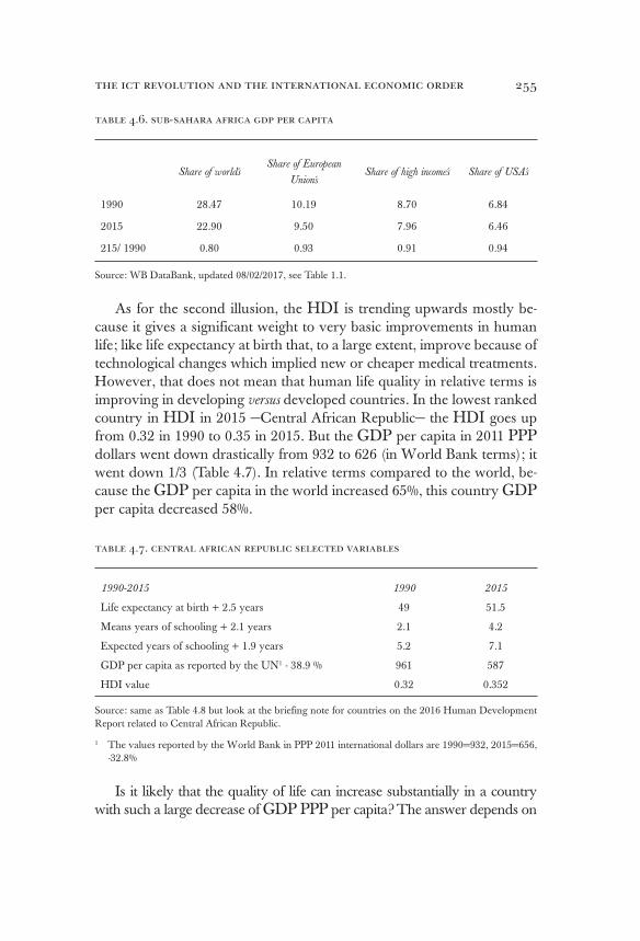
the ict revolution and the international economic order 255
table 4.6. sub-sahara africa gdp per capita
Share of world´s
Share of European
Union´sShare of high income´s Share of USA´s
1990 28.47 10.19 8.70 6.84
2015 22.90 9.50 7.96 6.46
215/ 1990 0.80 0.93 0.91 0.94
Source: WB DataBank, updated 08/02/2017, see Table 1.1.
As for the second illusion, the HDI is trending upwards mostly be-cause it gives a significant weight to very basic improvements in human life; like life expectancy at birth that, to a large extent, improve because of technological changes which implied new or cheaper medical treatments. However, that does not mean that human life quality in relative terms is improving in developing versus developed countries. In the lowest ranked country in HDI in 2015 —Central African Republic— the HDI goes up from 0.32 in 1990 to 0.35 in 2015. But the GDP per capita in 2011 PPP dollars went down drastically from 932 to 626 (in World Bank terms); it went down 1/3 (Table 4.7). In relative terms compared to the world, be-cause the GDP per capita in the world increased 65%, this country GDP per capita decreased 58%.
table 4.7. central african republic selected variables
1990-2015 1990 2015
Life expectancy at birth + 2.5 years 49 51.5
Means years of schooling + 2.1 years 2.1 4.2
Expected years of schooling + 1.9 years 5.2 7.1
GDP per capita as reported by the UN1 - 38.9 % 961 587
HDI value 0.32 0.352
Source: same as Table 4.8 but look at the briefing note for countries on the 2016 Human Development Report related to Central African Republic.
1 The values reported by the World Bank in PPP 2011 international dollars are 1990=932, 2015=656, -32.8%
Is it likely that the quality of life can increase substantially in a country with such a large decrease of GDP PPP per capita? The answer depends on
carlos obregón256
what we mean by life. If we want to measure how far is a country from oth-ers in terms of an international basket of goods, in this case the 2011 GDP per capita is a better indicator. The GDP per capita measures a country in relative terms against others and itself across time. There is no doubt that Central African Republic is much worse off in 2015 than in 1990 in these terms. But then, how come it improved the HDI? Because HDI measures the country with a set of minimum standards. This critique, however, does not mean that the Millennium Goals are irrelevant or that we should discon-tinue efforts to improve the HDI. Such efforts are very welcome; they do a lot of good to many people, but again, they are not enough.
Programs to improve the income distribution in developing countries are important. Social programs to fight extreme poverty and to improve the HDI index are welcome and necessary. But these programs are not sufficient. An economic development program is required. Its goal has to be that, in relative terms developing countries grow their GDP PPP per capita more than the developed countries. Development in terms of economic growth is required to improve in a sustainable long-term way human beings’ quality of life.
The global income distribution
The fact that the global income distribution has been improving recently should not be confused, as we said, with the statement that the poor countries are converging towards the rich ones. The global income distri-bution is an average —that has been heavily influenced by China due to the ICT revolution— but if we take China and India away, the rest of the world does no necessarily converge.
Will the world become more egalitarian? In the average, it most likely will. Although we cannot define the speed of convergence and there are many reasons to believe that it will slow down, such as:
1. Increasing protectionism in developed countries, mostly due to their refusal to grow their trade deficit indefinitely.
2. The uncertain political future in China.3. The uncertainty as to how well China will manage to become
a middle-income country.4. We do not know to what extent other large populated Asian
countries will manage the Asian Development Model properly.
the ict revolution and the international economic order 257
But even if convergence continues in the average at a proper speed. That does not mean poor countries are developing as they should —and much less that the world is growing near its potential.
The human development index and poverty
Sen’s thinking has influenced, as we said before, the United Nations De-velopment Goals which have been redefined in terms of developing ca-pabilities and opportunities for all individuals, and are measure by the Human Development Index (HDI)117. Table 4.8 presents how the HDI has performed in 1990 versus 2015. As it can be seen, it shows a big im-provement worldwide and even a larger improvement in Sub-Saharan Africa. How is it possible? What does the HID really measures? How does it differ from the GDP per capita? Should we use the GDP per capita or the HDI index to understand inequality?
The HDI in Sub-Saharan Africa improves more than the World from 1990 to 2015 (Table 4.8). This is an improvement, as we mentioned, against a set of minimum standards of living. However, if we look at poverty from 1990-2013 in Sub-Saharan Africa, there actually was an absolute increase (Table 4.5). Moreover, the fact that Sub-Saharan Africa is improving its minimum standards of living —because of global tech-nological reasons— does not mean that it is not becoming a less modern country in terms of the rest of the world. Despite its HDI improvement, Sub-Saharan Africa diverges from the whole world and from the West in 1990-2015, anyway we measure it (Table 4.6). That means that its quality of life compared with the rest of the world is going down. Both the HDI and the GDP per capita are relevant data. However, we must not confuse ourselves. We must be clear that improving the HDI index should be one of the global development goals, but it is not sufficient. The main goal has to be that Sub-Saharan Africa improves its quality of life in modern terms compared to others.
At a minimum, the world should implement an economic program aimed at developing the poor countries; but, the world could even go further than this. In the next section, we will argue that the developed economies should finance the development of the whole underdeveloped world; and that they would be the first beneficiaries of such a program.117 For a review of Sen’s proposals, see Obregon 2008a and 2014a.
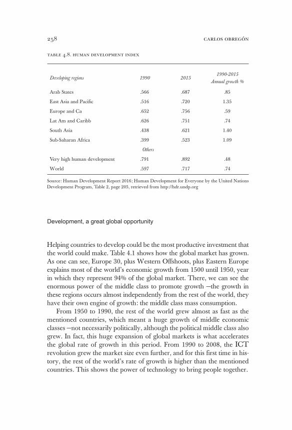
carlos obregón258
table 4.8. human development index
Developing regions 1990 20151990-2015
Annual growth %
Arab States .566 .687 .85
East Asia and Pacific .516 .720 1.35
Europe and Ca .652 .756 .59
Lat Am and Caribb .626 .751 .74
South Asia .438 .621 1.40
Sub-Saharan Africa .399 .523 1.09
Others
Very high human development .791 .892 .48
World .597 .717 .74
Source: Human Development Report 2016; Human Development for Everyone by the United Nations Development Program, Table 2, page 205, retrieved from http://hdr.undp.org
Development, a great global opportunity
Helping countries to develop could be the most productive investment that the world could make. Table 4.1 shows how the global market has grown. As one can see, Europe 30, plus Western Offshoots, plus Eastern Europe explains most of the world’s economic growth from 1500 until 1950, year in which they represent 94% of the global market. There, we can see the enormous power of the middle class to promote growth —the growth in these regions occurs almost independently from the rest of the world, they have their own engine of growth: the middle class mass consumption.
From 1950 to 1990, the rest of the world grew almost as fast as the mentioned countries, which meant a huge growth of middle economic classes —not necessarily politically, although the political middle class also grew. In fact, this huge expansion of global markets is what accelerates the global rate of growth in this period. From 1990 to 2008, the ICT revolution grew the market size even further, and for this first time in his-tory, the rest of the world’s rate of growth is higher than the mentioned countries. This shows the power of technology to bring people together.
the ict revolution and the international economic order 259
What particularly interests us in here is the fast growth of the markets in 1950 to 1990. There are two reasons: 1) the expansion of transporta-tion and communications technology due to the Second World War and 2) that the right institutional arrangement was implemented. The Mar-shall Plan aimed mainly at the recovery of Europe and Japan, but because technology has brought markets closer to each other, Europe and Japan’s growth stimulated the growth of the whole world. These explains that the world GDP per capita without the middle class’ annual growth rate is almost equal to the middle class’, in Table 4.1118.
The impact of the ICT revolution, in terms of bringing the markets together, as we have pointed out, has been very powerful and it will con-tinue. What will the adequate institutional arrangement to foster future economic growth be? What will today’s equivalent to the old Marshall Plan be, that could trigger a much faster worldwide growth? The answer might be an economic program at the global level to modernize the under-developed economies, financed by the developed countries. Why should they do it? Because they would be key beneficiaries of such a program.
118 After all, there was wisdom in the Stationary State of the classical economists. Technol-ogy impacts society in several ways, but four key areas are medical technology, technol-ogy in agricultural production, technology in manufacturing production and technology in communications and transportation. Medical technology decreases infant mortality and in-creases life expectancy, therefore fosters population growth. The increase demand for food has to be matched with technology in agricultural production, which historically has been so succesful that less and less human labor is required. Therefore, people move to the cities that provide the first restrain to population growth, because the number of descendants per family goes down in the ciites. Urban life requires technology in manufacturing to go up and societies enter the positive cycle that Smith described: as the market gets bigger, due to trade and growth of the middle class, mass production fosters technological innovations in manufacturing. Transportation and communications technology bring markets together, therefore increases Smith’s innovation factor and the expansión of technology in manu-facturing. But the process is a delicate one, protectionism is a menace because it decreases trade and slows innovations in manufacturing technology which is dangerous —particularly because the population continues to grow, mainly due to new developments in medical technology. Historically, Smith’s positive technology cycle has been more powerful than Malthus’ population exponential growth, but it is of paramount importance that technol-ogy is permitted to work properly. The world has to allow the ICT technology deliver the productivity increases that it can. The Malthus-Smith cycles can be seen historically if we compare the world in period 1913-1950 where trade slows down, versus 1870-1913 and 1950-2008 where trade expands. Global population grows annually at 0.79% in 1870-1913, and GDP per capita at PPP 1990 dollars grows at 1.31%. In 1913-1950, trade slows down and the population continues growing at an anual rate of 0.93%. The consequence is that GDP per capita annual growth rate slowed down to 0.88% annual rate. In 1950 to 2008, as trade expands sustantially due to improvements in transportation and communications technology, the annual rate of growth of GDP per capita is 2.24%. This allows for a more rapid population growth of 1.71% annually.
carlos obregón260
The Marshall Plan ended up being excellent for the world, particu-larly for the USA. A truly well conceived development plan to modernize the world would benefit everyone, especially the developed countries. Why does it not happen then? The answer, as we have been saying, is game theory. There are no institutions which can guarantee that only pareto moves will be made, and building them is costly; therefore, maxi-mizing its individual interests, developed countries sacrifice the potential for a much rapid global growth. But given the opportunity that the ICT revolution presents, it will be a critical point in history to build the previ-ously mentioned institutions.
We do not want to be called idealists, we believe that a global econom-ic development program like the one we are proposing is very unlikely. However, it is our duty to point out its convenience. After all, nobody would have believed after the First World War that the Marshall Plan could happen after the Second World War. In any case, it is clear that eco-nomic development is not a solved issue and it will not be solved by itself.
What should be the IMF’s role in a global development program like the one we just proposed? Based on an economic development program agreed with each underdeveloped economy, the IMF could provide fi-nancial support to reduce the volatility of the exchange rates of devel-oping economies; exchange rate volatility whose risk will become the IMF’s. In other words, the IMF will support the exchange rates within a pre-agreed bands. They will become semi-fixed exchange rates. If a developing economy has a significant external shock, the IMF will agree on a new band for its exchange rate. This will imply that the developing country is free to use its autonomous monetary policy —because within the band, the exchange rate is floating and also changing the band is pos-sible. But the excess exchange rate volatility related to fears of financial crisis that prevents planning for the future will disappear.
As a final point, we would like to comment that markets enlarge par-tially due to the uneven income distributions, because even though the average citizen of a given country may not be able to become a global consumer of products with frontier technology, some population deciles might. Table 4.9 presents the case of China (2012) and the United States (2013). In 2012, two Chinese deciles had a higher income per capita than the USA’s second bottom decile in 2013, and one decile had it higher than the USA’s fourth and fifth bottom deciles. There are many ways to think these numbers, but whichever we choose, it is clear that technology incor-porates more and more people to the global markets and that this process

the ict revolution and the international economic order 261
clearly speeds up global economic growth. A development program like the one we have just described will greatly accelerate such a process.
table 4.9. gdp per capita (2011 ppp constant international dollars) per decile
CHINA (2012) VS USA (2013)
DECILES
I II III IV V VI VII VIII IX X
CHINA
2285 3544 4793 6086 7479 9073 11045 13754 18357 35031
USA
8671 17343 23260 29228 35706 43051 51978 63863 82889 153995
Source: WB 2016 from United Nations, see Table 2.28. GDP per capita 2011 PPP constant international dollars from WB DataBank, see Table 1.1.
The international legal framework, fiscal paradises disappearance or close supervision and control of financial flows as required instruments to control tax evasion, corruption, terrorism and criminal activities in general
The world’s institutions are not well prepared for the huge changes that the ICT revolution has been bringing about. When many legal and illegal activities can be globalized and managed from offshore, the absence of a clear international law with international courts and judges is a big minus. But again, national interest, as expected by game theory, have blocked consistently any serious advance in this direction. The United States and other developed nations insist in seeing their national local law as the global standard, and their judges and courts as having an international reach. Of course, there is a sophisticated international law today, but it is insufficient when the main participants do not recognize the international courts.
One of the biggest consequences of such an international legal vac-uum has been the growth of fiscal paradises, which today intermediate
carlos obregón262
a significant percentage of the foreign direct investment that enters into the developed countries (see Table 2.1). This is bad news because a large portion of this money does not have licit origins. At best, it does not pay taxes properly in the country of origin, and at worse, it is money from criminal activities and terrorist groups. It has become vey difficult for governments to increase taxes to capital income substantially, or inheri-tance taxes, because capital can escape the country through fiscal para-dises and ends up investing in other country. This has become a serious restriction in implementing a redistributive fiscal policy. This situation is unfair for those that do pay their tax share. The global trafficking of people, arms, and drugs could be diminished largely if there was not a way for their financial flows to be hidden. Thus, the disappearance or strict supervision of fiscal paradises would bring to the world many ben-efits, but it cannot occur as long as there is not full global coordination in legal issues —through laws, courts, and judges accepted by all the nations.
Global sustainability and the possibility of a global demographic policy
The recent USA’s announcement of its intentions to abandon the Paris Accords has shown how fragile the sustainability policies really are. Here, like in many previous topics, national interest and the wrong games played have prevailed over optimizing the common interest. It is expected that there will be future advances in this area, but they will always be limited as long as there is not a proper international common legal arrangement. As for the global demographic policy, like many other policies, it has been traditionally delegated to the countries, and it will continue being this way if there is not a worldwide coordinated development program.
conclusion
The ICT revolution has brought the world closer together as never be-fore and the institutional global arrangement has not been able to re-spond efficiently. In this chapter, we have reviewed the goals that a future global economic order should have, and we have arrived at the conclu-sions that follow.
the ict revolution and the international economic order 263
The actual floating exchange rates - free capital flows regime is the adequate one because its flexibility is required due to the rapid ICT revo-lution changes. But, because finances have become global, it is no longer enough for a Central Bank to define its monetary policy in traditional terms. In addition to setting the Central Bank’s rate and buying or sell-ing government bonds, today the Central Banks have to enter the credit realm —getting very close to what traditionally had been fiscal policy. En-tering credit means getting guidance by a set of macroprudential policies. Because credit is globalized today, for the Central Banks to enter credit they have to coordinate efficiently at the global level. In addition, for these coordinating processes to be permanent in the future, it is recom-mended to strengthen the role of the global financial institutions.
The ICT revolution has globalized many activities, both legal and illegal. It has allowed the flourishing of fiscal paradises, consequently, countries have lost their redistributive fiscal policy capability and money laundering and illegal financial flows have grown up substantially. How-ever, disappearing or supervising closely the fiscal paradises will not be easy in a world that does not have accepted international laws to be used in common international courts with accepted international judges.
Democracy means that national governance has increased in most of the developed countries, while global governance has decayed. Conse-quently, the world today is a very unjust place, more unequal in terms of income distribution that the least egalitarian countries on earth.
There are misleading positive indicators that must be reinterpreted correctly. The global income distribution is improving recently, extreme poverty is going down quickly and the HDI has a clear upward trend. However, the improvement in the global income distribution is conse-quence of the isolated development of a selected group of countries; it is not a global phenomenon. Convergence between rich and poor countries is not general. Most of the reduction in extreme poverty happened in East Asia and it is not a global phenomenon. In Sub-Saharan Africa, for example, the number of extreme poor people has increased in absolute numbers. The HDI upward trend is mostly due to the heavy weight given to minimum standards of living —variables such as life expectancy at birth, mean years of schooling and expected years of schooling; these variables improve mostly due to technological advances in medicine and other fields. But despite the HDI improvement, the real standard of living is clearly going down in countries like Central African Republic, whose GDP PPP per capita went down in 1990-2015, 33%. In relative

carlos obregón264
terms, the Central African Republic GDP per capita fell 58% respect to the world’s and the Sub-Saharan Africa fell 13%.
The world is not solving properly the problems of poverty, improve-ment in human quality of life and income distribution. Something else has to be done. At a minimum, a developing program for poor countries should be implemented, and ideally —which we recognize will be very difficult to accomplish—, an economic program to modernize the entire underdeveloped world should be launched. Such an ambitious program would be the right way to use the potential of the ICT revolution to sig-nificantly improve the world’s rate of economic growth.

[265]
POLICY ALTERNATIVES FOR DEVELOPED
AND DEVELOPING COUNTRIES
In the previous chapter, we discussed policies from the world’s perspec-tive, but many of them, despite their convenience, have low probability of implementation because of the games involved in the competition be-tween nations. The world is ruled by game theory and not by traditional neoclassical optimizing behavior. The world is defined mostly by nation-al interests and, only occasionally, by coordinated moves. A country may have policies towards promoting coordinated moves but cannot assume that it will be successful and that such coordinated moves will occur —it has to optimize its national interest. In this chapter, we limit ourselves to the perspective of an individual country’s selfish national interest. In what follows, we will review some of the policies that developed and developing countries should have.
Along the previous chapters, we have been building a scenario that provides us with likely parameters that all the countries will face. Coun-tries will have to optimize their individual policies against these likely scenarios. We have discussed that automation will develop further and will put extra pressure on low and medium skill workers from developed countries. The ICT revolution will continue and will likely be strength-ened in the future by telerobotics, telepresence and virtual migration119. Developed countries will lose more and more competitiveness at the global level in low to medium skill workers, and they will remain com-petitive in high-skill workers and robotized activities.
The ICT revolution makes migration less needed, as firms find low wage labor offshore. Migrant labor supply will be reduced in the developed countries, but it will be more than compensated by the labor from offshore locations120. Therefore, it is clear that low to medium skill workers in de-veloped countries will continue to be under pressure, both from offshore competition and from automation. Anti-migration policies will continue because they are a natural consequence of the ICT revolution, hence, de-
119 For more on this see Baldwin 2016, chapter ten.
120 Peters 2017.
carlos obregón266
veloping countries may find increasingly difficult to rely in migration as a solution. It is likely that national interest in the developed countries will prevent the financing of the global economic program to modernize the underdeveloped world, that we suggested in the previous chapter, so:
a) Trade barriers in agricultural products will continue to be used by developed countries.
b) Trade preferences given to poor countries will remain very limited.
c) Property rights will continue to be defended by developed countries through agreements such as TRIPS (agreements on Trade-Related Aspects of Intellectual Property).
d) Development aid will continue to be very limited and fragile.It is very unlikely that, in the short-term, fiscal paradises will be close-
ly supervised or disappear. Therefore, fiscal reforms based upon taxation of capital income and inheritance income will have limited potential. The stock market in the developed countries will boom again as huge interna-tional companies take advantage of the ICT revolution, and executive’s salaries in the financial sector will remain very high (it is already happen-ing in USA). Asian institutions (and maybe other developing countries) will become more and more competitive as it has happened already —and this new level of competitiveness cannot be confronted through trade restrictions. Large populated countries in Asia, such as Vietnam or Ban-gladesh, are better positioned than other countries to partially replace China if needed; but other developing countries are aware of what is happening and will try to compete. Among these other countries, Mexico is particularly well position.
With the previous scenario in mind, we will discuss the policies that developed and developing countries must adopt.
policies for developed countries
The main economic problems of any economy are growth and income distribution. And, as we have been arguing, growth is compatible with many distributions of income. Therefore, there is no need to choose one goal or the other, they can be reached together.
There are only three sources of growth: labor, capital and the process of production that puts them together. However, none of them is a static
267policy alternatives for developed and developing countries
component. The three are subject of technological innovations; in addi-tion, labor quality changes by education. If the developed countries want to continue growing, they need to bet on technological innovations and in higher education. They have to train their population so that they can incorporate themselves to high skill tasks. Within-the-job-training should be encouraged. They should modernize their economies’ infrastructure by using some of the low to medium skill labor that becomes available due to the ICT technological revolution.
Well understood, the ICT revolution is a great opportunity for de-veloped countries. In terms of economic growth, the ICT revolution means higher global productivity, which, specifically for the developed countries, translates into cheaper goods for the population and higher profits for the companies involved. The higher global productivity trans-lates into lower inflation expectations, the higher global savings into a lower real interest rate. Both factors together lower nominal interest rates, which increase the credit capacity of the middle class in developed countries and substantially improves its standard of living. The policies for developed economies are summarized below in Table 5.1 and 5.1a.
What the developed countries cannot do is to oppose the ICT tech-nological revolution; opposing technological revolutions is futile and counterproductive. A developed nation cannot compete against low wage underdeveloped countries in manufacturing production that involves low to medium skill labor. Attempts to do it by creating trade barriers will only worsen the situation in the end. The country that closes itself through trade barriers and anti-migration policies will just become less and less productive in relationship to the rest of the world. Developed countries cannot go backwards; they have to continue moving forward. The way to go is to create the proper institutional arrangement to grasp the potential productivity increases that the new technological revolution can bring. The point is to not oppose the ICT revolution, but use it in the favor of the developed country involved.
As for trade policies, the developed countries should sign convenient regional agreements seeking gains in global competitiveness, but they have to avoid protectionism. Nationalism and protectionism will not im-pede the ICT revolution to go on but will damage the medium and long- term interest of the country involved. On the contrary, the developed countries must place themselves on the vanguard of the ICT revolution and try to be competitive in innovative information, communications, robot technology and others.
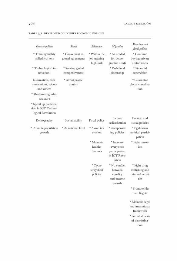
carlos obregón268
table 5.1. developed countries economic policies
Growth policies Trade Education MigrationMonetary and
fiscal policies
* Training highly skilled workers
* Convenient re-gional agreements
* Within the job training high skill
* As needed for demo-
graphic needs
* Continue buying private sector assets
* Technological in-novation:
* Seeking global competitiveness
* Redefined citizenship
* Financial supervision
Information, com-munications, robots
and others
* Avoid protec-tionism
* Guarantee global coordina-
tion
* Modernizing infra-structure
* Speed up participa-tion in ICT Techno-logical Revolution
Demography Sustainability Fiscal policyIncome
redistributionPolitical and social policies
* Promote population growth
* At national level * Avoid tax evasion
* Compensat-ing policies
* Egalitarian political partici-
pation
* Maintain healthy finances
* Increase everyone´s
participation in ICT Revo-
lution
* Fight terror-ism
* Coun-tercyclical policies
* No conflict between equality
and income growth
* Fight drug trafficking and criminal activi-
ties
* Promote Hu-man Rights
* Maintain legal and institutional
framework
* Avoid all sorts of discrimina-
tion
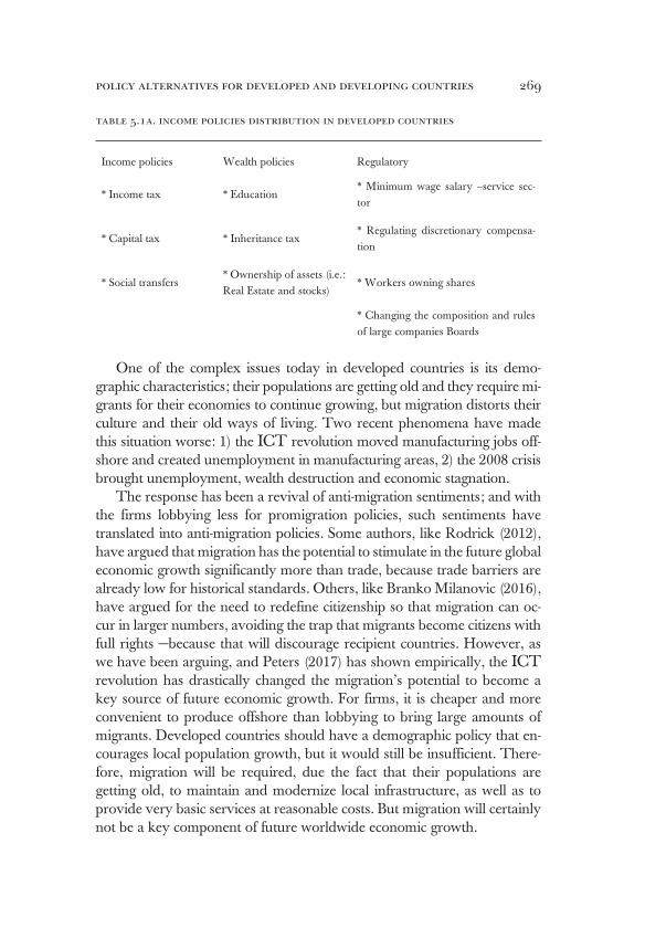
269policy alternatives for developed and developing countries
table 5.1a. income policies distribution in developed countries
Income policies Wealth policies Regulatory
* Income tax * Education* Minimum wage salary –service sec-tor
* Capital tax * Inheritance tax* Regulating discretionary compensa-tion
* Social transfers* Ownership of assets (i.e.: Real Estate and stocks)
* Workers owning shares
* Changing the composition and rules of large companies Boards
One of the complex issues today in developed countries is its demo-graphic characteristics; their populations are getting old and they require mi-grants for their economies to continue growing, but migration distorts their culture and their old ways of living. Two recent phenomena have made this situation worse: 1) the ICT revolution moved manufacturing jobs off-shore and created unemployment in manufacturing areas, 2) the 2008 crisis brought unemployment, wealth destruction and economic stagnation.
The response has been a revival of anti-migration sentiments; and with the firms lobbying less for promigration policies, such sentiments have translated into anti-migration policies. Some authors, like Rodrick (2012), have argued that migration has the potential to stimulate in the future global economic growth significantly more than trade, because trade barriers are already low for historical standards. Others, like Branko Milanovic (2016), have argued for the need to redefine citizenship so that migration can oc-cur in larger numbers, avoiding the trap that migrants become citizens with full rights —because that will discourage recipient countries. However, as we have been arguing, and Peters (2017) has shown empirically, the ICT revolution has drastically changed the migration’s potential to become a key source of future economic growth. For firms, it is cheaper and more convenient to produce offshore than lobbying to bring large amounts of migrants. Developed countries should have a demographic policy that en-courages local population growth, but it would still be insufficient. There-fore, migration will be required, due the fact that their populations are getting old, to maintain and modernize local infrastructure, as well as to provide very basic services at reasonable costs. But migration will certainly not be a key component of future worldwide economic growth.
carlos obregón270
The monetary policy in developed countries should continue to be heterodox; Central Banks should continue buying private sector assets. This will maintain them close to what is happening in the real markets and will allow for an efficient financial supervision. But because credit is already globalized, developed countries must ensure that proper global coordination takes place in money and finances to avoid a future interna-tional financial crisis.
As we have argued, nationalism and protectionism are related to the damages of the 2008 financial crisis and not to the medium-term income distribution changes. But nonetheless, losers of the ICT revolution in the developed economies should be compensated.
Developed countries must rip the huge economic growth benefits as-sociated with the ICT revolution and they should compensate locally at the losers. The aim is to allow everybody to participate in the huge benefits brought about by the ICT revolution. There are three sets of policies that can be enacted to influence the national income distribution:
1. Policies to distribute income, such as income tax, capital taxes and social transfers.
2. Wealth policies trying to even out the assets with which each person enters his economic activity, such as education train-ing, inheritance taxes, and policies to broaden the ownership of stocks and real estate.
3. Regulatory policies, such as minimum wage, contractual con-ditions affecting particularly the service sector, and regulating discretionary compensation in large multinationals and banks.
Some of these policies are national decisions, but others require interna-tional cooperation that may not be obtained. Capital and inheritance taxes require global coordination to get rid of the fiscal paradises, which, as we have argued, at this point seems very unlikely. Therefore, without ample use of these two key instruments, the national policies will have to focus in the other instruments. Personal income taxes and social transfers can still be used in many countries. Education training —particularly job related— is much needed and can be done. The broadening of the stocks ownership and real estate can be achieved. Increasing the minimum wage and the contrac-tual conditions, particularly related to the service sector, is quite possible. Regulation of top executives’ salaries should not be done directly —because the government should not intervene with market’s efficiency— but the gov-ernments can influence them indirectly by resolving some market structural failures that maintain them unjustifiably high. We will explore with more
271policy alternatives for developed and developing countries
detail each one of these policies, but the point to make now is that even with the present limited global coordination it is quite possible for a developed country to compensate the losers. Thus, helping the losers should not be used as an excuse to foster protectionist policies.
The goals of a fiscal policy in general are to promote an egalitarian society, to avoid tax evasion, to enact countercyclical policies if needed and to maintain healthy state finances. Fiscal paradises limit the scope of capital and inheritance taxes, restricting very much the possibilities of the fiscal policies to promote an egalitarian society. Although there is still room for egalitarian policies through the personal income tax and through social transfers and in addition, as we had seen in points 2) and 3) above, other policies (not related to the fiscal policy) can be used. Also, fiscal paradises significantly difficult the task of preventing tax evasion.
Proper countercyclical policies require international coordination if the crisis is global, but for the most part, it can be defined at the national level. Healthy state finances are a goal that can also normally be achieved at the national level.
Political security and social policies are guided to obtain egalitarian political participation, to avoid discrimination of all sorts, to promote hu-man rights, to maintain a legal institutional arrangement, to fight drug trafficking and criminal activities and to fight terrorism. Many of these goals can be achieved locally but others require international coordina-tion, which, as we have seen, today is insufficient. As long as fiscal para-dises can be used for illegal money transfers, it will be almost impossible to efficiently fight drug trafficking, terrorism and other criminal activities. Finally, environmental sustainability should be a national goal ant it can be partially achieved at this level; but without global coordination, it can-not be fully achieved.
Since this general policy frame applies for all the developed countries, in what follows we will discuss only briefly specific policies for the USA, Europe, and Japan.
The United States
The USA has several distinctive assets such as its global political and mili-tary leadership. It is by far the wealthiest society on earth; its consump-tion is definitive in defining the future direction of the ICT revolution. It
carlos obregón272
is the leader in developing ICT technology and in global finances. The principal task of any set of policies designed must be for the USA to main-tain its privileged position. Is there anyway it can lose it? Yes, it will lose it if it opposes the ICT revolution. The point is very simple: the USA cannot survive in the competitive global market by refusing migrants and the offshore manufacturing of the USA’s companies at the same time —because that means producing manufacturing goods at higher price com-pared to others. Which will reduce USA competitiveness and initiate the USA’s decay.
What specific emphasis should the USA’s policies have? Of all coun-tries, the USA is the one with a greater need to fully ride the ICT revolu-tion. It has to continue to be in the frontier for information technology and communications and needs to speed up its competitiveness in robot technology. Telerobotics, telepresence, virtual migration, and automa-tion are coming; the USA has to maintain itself in the frontier. It has to intensify, as much as possible, offshore manufacturing. Growth for the USA must come from:
a) Continuing developing its leadership in innovative ICT technology; and bet on new technologies to come, like auto-mation or space technology121.
b) Maintaining its leadership in global finances. c) From manufacturing offshore —maintaining home manufac-
turing services. d) From the service sector at home. To promote economic growth, it is a good idea to renew the infra-
structure in highways, buildings and so on. There is room to do this but not at higher prices than the rest of the world. If the USA takes this route, it will create jobs for US citizens —some of the low to medium skill labor unemployed by the ICT revolution could be used here— but will also have to hire migrants if it wants to do it at reasonable prices. The country will buy inputs from local USA companies but it also has to increase its
121 In terms of economic growth, the historical modern record of the USA is very good. From 1820-2008 it grew at 1.73% versus the world’s 1.21% (see Table 5.2). From 1950 to 1990, the world benefited a lot from the Marshall Plan and from the war’s economic recovery and it grew at 2.25%, but the USA also benefited a lot. Its rate of growth went from 1.61% in 1913-1950 to 2.24% in 1950-1990. From 1990-2008 the USA grows at 1.66%, while the world’s grows at 2.20%. But that does not mean that the USA growth is low or inadequate. The USA is a mature economy and grew as such and very close to its long-term growth average of 1.72%. Other mature economies grew even less than the USA, Europe 12 grew 1.57% and Japan 1.08%. What is surprising is not the USA growth, but the high growth rate of the rest of the world and that is due to China and the ICT revolution.

273policy alternatives for developed and developing countries
imports from low wage countries. No country can survive in a globalized world, building its infrastructure at very high prices. Therefore, building infrastructure does not change the medium to long-term fact that the jobs in the service sector will have to increase and that better conditions in these jobs will have to be guaranteed.
table 5.2. usa market share1 and relative growth versus
the world in gdp per capita and population
YearUSA Market
share %Period
GDP per capita
(annual growth rate)
Population
(annual growth rate)
USA World USA World
1500 - 1500-1820 0.36 0.051 0.50 0.27
1820 3.26 1820-1870 1.34 0.540 2.83 0.41
1870 16.59 1870-1913 1.82 1.310 2.08 0.79
1913 28.62 1913-1950 1.61 0.880 1.21 0.93
1950 42.76 1950-1990 2.24 2.250 1.25 1.85
1990 27.75 1990-2008 1.66 2.200 1.09 1.30
2008 22.90
1820-1990 1.73 1.210 1.91 0.96
1820-2008 1.72 1.300 1.83 0.99
Source: Maddison 2009, see Table 1.1.
1 Methodology: USA market share is defined as [(USA GDP per capita - Africa GDP per capita) * USA Population] / [(World GDP per capita - Africa GDP per capita) * world population]. Therefore, this market share relates to somewhat sophisticated goods. See Table 4.4.
Trade and growth are always related. It is true that the USA has not had proper access to the Asian markets, particularly to Japan and to China due to the Asian Development Model. Thus, it is natural for the USA to want to reciprocate —but it cannot do it producing at high pric-es and creating trade barriers. Its opportunity is Mexico and NAFTA, which later on could be expanded to other Latin American countries. If the USA wants to remain competitive, it needs to produce with low wage labor and it can find it in the south. The best thing for the world is mul-tilateral agreements; the best thing for the USA is a regional agreement like NAFTA, which could allow it to negotiate better with China, Japan, and Europe.
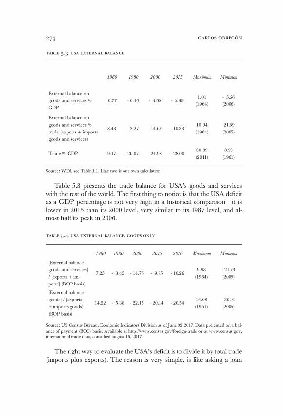
carlos obregón274
table 5.3. usa external balance
1960 1980 2000 2015 Maximum Minimum
External balance on goods and services % GDP
0.77 - 0.46 - 3.65 - 2.891.01
(1964)- 5.56 (2006)
External balance on goods and services % trade (exports + imports goods and services)
8.43 - 2.27 - 14.63 - 10.3310.94 (1964)
-21.59 (2005)
Trade % GDP 9.17 20.07 24.98 28.0030.89 (2011)
8.93 (1961)
Source: WDI, see Table 1.1. Line two is our own calculation.
Table 5.3 presents the trade balance for USA’s goods and services with the rest of the world. The first thing to notice is that the USA deficit as a GDP percentage is not very high in a historical comparison —it is lower in 2015 than its 2000 level, very similar to its 1987 level, and al-most half its peak in 2006.
table 5.4. usa external balance. goods only
1960 1980 2000 2015 2016 Maximum Minimum
[External balance goods and services] / [exports + im-ports] (BOP basis)
7.25 - 3.45 - 14.76 - 9.95 - 10.269.93
(1964)- 21.73 (2005)
[External balance goods] / [exports + imports goods] (BOP basis)
14.22 - 5.38 - 22.15 - 20.14 - 20.5416.08 (1961)
- 30.01 (2005)
Source: US Census Bureau, Economic Indicators Division as of June 02 2017. Data presented on a bal-ance of payment (BOP) basis. Available at http://www.census.gov/foreign-trade or at www.census.gov, international trade data, consulted august 16, 2017.
The right way to evaluate the USA’s deficit is to divide it by total trade (imports plus exports). The reason is very simple, is like asking a loan
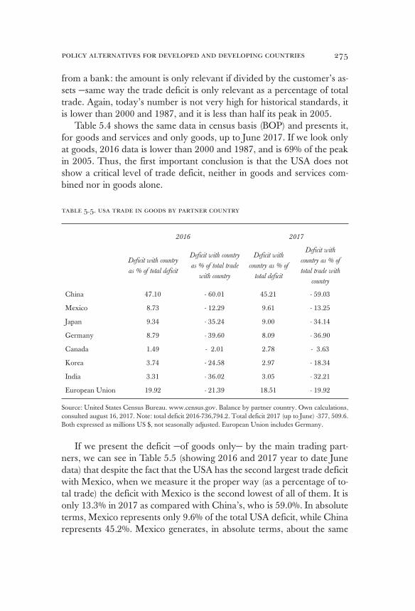
275policy alternatives for developed and developing countries
from a bank: the amount is only relevant if divided by the customer’s as-sets —same way the trade deficit is only relevant as a percentage of total trade. Again, today’s number is not very high for historical standards, it is lower than 2000 and 1987, and it is less than half its peak in 2005.
Table 5.4 shows the same data in census basis (BOP) and presents it, for goods and services and only goods, up to June 2017. If we look only at goods, 2016 data is lower than 2000 and 1987, and is 69% of the peak in 2005. Thus, the first important conclusion is that the USA does not show a critical level of trade deficit, neither in goods and services com-bined nor in goods alone.
table 5.5. usa trade in goods by partner country
2016 2017
Deficit with country
as % of total deficit
Deficit with country
as % of total trade
with country
Deficit with
country as % of
total deficit
Deficit with
country as % of
total trade with
country
China 47.10 - 60.01 45.21 - 59.03
Mexico 8.73 - 12.29 9.61 - 13.25
Japan 9.34 - 35.24 9.00 - 34.14
Germany 8.79 - 39.60 8.09 - 36.90
Canada 1.49 - 2.01 2.78 - 3.63
Korea 3.74 - 24.58 2.97 - 18.34
India 3.31 - 36.02 3.05 - 32.21
European Union 19.92 - 21.39 18.51 - 19.92
Source: United States Census Bureau. www.census.gov. Balance by partner country. Own calculations, consulted august 16, 2017. Note: total deficit 2016-736,794.2. Total deficit 2017 (up to June) -377, 509.6. Both expressed as millions US $, not seasonally adjusted. European Union includes Germany.
If we present the deficit —of goods only— by the main trading part-ners, we can see in Table 5.5 (showing 2016 and 2017 year to date June data) that despite the fact that the USA has the second largest trade deficit with Mexico, when we measure it the proper way (as a percentage of to-tal trade) the deficit with Mexico is the second lowest of all of them. It is only 13.3% in 2017 as compared with China’s, who is 59.0%. In absolute terms, Mexico represents only 9.6% of the total USA deficit, while China represents 45.2%. Mexico generates, in absolute terms, about the same
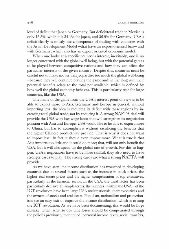
carlos obregón276
level of deficit that Japan or Germany. But deficit/total trade in Mexico is only 13.3%, while it is 34.1% for japan, and 36.9% for Germany. USA’s deficit clearly is mostly the consequence of trading with countries with the Asian Development Model —that have an export-oriented bias— and with Germany, which also has an export oriented economic model.
When one looks at a specific country’s interest, inevitably, one is no longer concerned with the global well-being, but with the potential games to be played between competitive nations and how they can affect the particular interests of the given country. Despite this, countries must be careful not to make moves that jeopardize too much the global well-being —because they will continue playing the game and, in the long run, their potential benefits relate to the total pot available, which is defined by how well the global economy behaves. This is particularly true for large countries, like the USA.
The name of the game from the USA’s interest point of view is to be able to export more to Asia, Germany and Europe in general, without importing less; the idea is reducing its deficit with these regions by in-creasing total global trade, not by reducing it. A strong NAFTA deal will provide the USA with low wage labor that will strengthen its negotiation position with Asia and Europe. USA would like to be able to export more to China, but has to accomplish it without sacrificing the benefits that the higher Chinese productivity provide. That is why it does not want to import less —in fact, it should even import more. What is true is that Asia imports too little and it could do more; that, will not only benefit the USA, but it will also speed up the global rate of growth. For this to hap-pen, USA’s negotiators have to be more skillful, they also need to have stronger cards to play. The strong cards are what a strong NAFTA will provide.
As we have seen, the income distribution has worsened in developing countries due to several factors such as the increase in stock prices, the higher real estate prices and the higher compensation of top executives, particularly in the financial sector. In the USA, the third factor has been particularly decisive. In simple terms, the winners —within the USA— of the ICT revolution have been large USA multinationals, their executives and the owners of stocks and real estate. Populism, nationalism and protection-ism see an easy exit to improve the income distribution, which is to stop the ICT revolution. As we have been documenting, this would be huge mistake. Then, what to do? The losers should be compensated through the policies previously mentioned: personal income taxes, social transfers,
277policy alternatives for developed and developing countries
educating and training high skill workers, broadening assets ownership of stocks and real estate, increasing the minimum salary and improving con-tractual conditions, particularly, as it relates to the service sector.
Compared with Europe, the USA still has space for egalitarian poli-cies through personal income taxes and through social transfers, and it should use it. But given the fact that only these two fiscal instruments are fully available —because the usage of capital income taxes and inheritance taxes is limited due to fiscal paradises—, the other available egalitarian policies should also be used.
At the end, the adjustment that the ICT revolution is bringing to the USA inevitably means that the service sector will grow, that is why given better contractual conditions to workers in this sector is a good idea, as well as increasing the minimum salary and giving higher education and on-the-job-training for higher skill labor is a most. Broadening the owner-ship of stocks and real estate can be achieved by several means. One of the ways to do it is to foster workers’ ownership of his own company’s stocks by law. The other is to create large diversified stock funds with two characteristics: a) a government insurance of, let us say 90% of principal, with a minimum investment period of five years, b) worker’s possibility to obtain loans against the fund when needed up, to let us say 40% of the investment. Investing in these large funds will be partially mandatory and partially voluntary. Providing liquidity and insurance will make stock in-vesting very popular, therefore, voluntary investment will be large. Real estate can actually be acquired through investment funds. In relationship to the high salaries of top executives, they should not be regulated, but a structural problem in relationship to the companies’ boards composi-tion should be solved. In the companies’ boards there should be both regulators and enough board members representing small stockholders and investment funds. Plus, the responsibilities of the boards should be extended. One of the problems today in the USA is that large companies’ boards are conformed by chairman of other large companies, which cre-ates a situation where nobody wants to criticize the big salary of another because it runs the risk that his own salary will be questioned.
In terms of migration, it must be understood that migrants in the USA are not the cause of manufacturing unemployment. Migrants per-form low skill services and agricultural related work. The manufactur-ing unemployment phenomenon is fully related to the ICT revolution and cannot be influenced by anti-migration policies. The US has been very inconsistent and has not been able to delineate a definitive migration
carlos obregón278
policy. The reason: a divided country in which part of the population receives the benefits of the migrants while others are culturally defensive and against migration. It is true that a minority, especially of very low skill workers, suffers from the migrant’s competition, but they are too few to make a difference. The case against migration is culturally and ideo-logically driven. However, an evident fact is that the USA cannot survive without migrants. Migration has been one of the key reasons of the long-term USA economic growth achievement (see Table 5.2). Therefore, a solution is urgently needed.
For the USA in particular, Milanovics’s idea of partial citizenship may be a good solution because it will actually clarify today’s migrant’s status —giving them the possibility to travel in and out without being treated like criminals. It is much better to recognize explicitly that they do not have full rights and spell which rights do they have than the actual situ-ation —which is not only inhuman but very costly in economic terms for the USA. Migrants do not produce at their full potential because they spend too much energy hiding or fighting for his rights. Border security is expensive and deporting costs too. A well define policy would be very much welcome, but just hardening conditions to try to prevent migrants to cross the border will not solve anything.
The USA, due to its worldwide leadership, should become more aware of the need for better global coordination. The ICT revolution has brought the world closer together than ever before. A technological-ly globalized world is in many ways incompatible with a world that pre-tends to be managed only through games based on national interests. There are just too many contradictions arising. Fiscal paradises make it very difficult to impose higher capital and inheritance taxes and make it almost impossible to fight efficiently against corruption, tax evasion, drug trafficking, other criminal activities and terrorism. Environmen-tal sustainability requires world’s coordination. It is unbelievable that the USA is moving backwards instead of forward by abandoning the Paris Accord. Monetary and financial stability, and efficient trade, also require global coordination. Even the pursue of human rights requires it. And, of course, the development problem, as we have been arguing, will not be solved without such coordination. The world needs much more global coordination, not less. The USA should use his leader’s role to promote it; the problem is that the USA is not understanding and it is not doing it. The USA mistakes will be costly both for the USA and for the world.
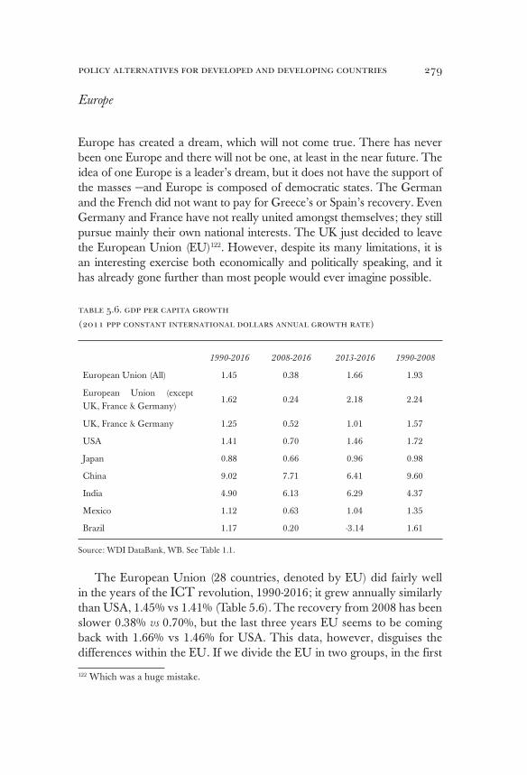
279policy alternatives for developed and developing countries
Europe
Europe has created a dream, which will not come true. There has never been one Europe and there will not be one, at least in the near future. The idea of one Europe is a leader’s dream, but it does not have the support of the masses —and Europe is composed of democratic states. The German and the French did not want to pay for Greece’s or Spain’s recovery. Even Germany and France have not really united amongst themselves; they still pursue mainly their own national interests. The UK just decided to leave the European Union (EU)122. However, despite its many limitations, it is an interesting exercise both economically and politically speaking, and it has already gone further than most people would ever imagine possible.
table 5.6. gdp per capita growth
(2011 ppp constant international dollars annual growth rate)
1990-2016 2008-2016 2013-2016 1990-2008
European Union (All) 1.45 0.38 1.66 1.93
European Union (except UK, France & Germany)
1.62 0.24 2.18 2.24
UK, France & Germany 1.25 0.52 1.01 1.57
USA 1.41 0.70 1.46 1.72
Japan 0.88 0.66 0.96 0.98
China 9.02 7.71 6.41 9.60
India 4.90 6.13 6.29 4.37
Mexico 1.12 0.63 1.04 1.35
Brazil 1.17 0.20 -3.14 1.61
Source: WDI DataBank, WB. See Table 1.1.
The European Union (28 countries, denoted by EU) did fairly well in the years of the ICT revolution, 1990-2016; it grew annually similarly than USA, 1.45% vs 1.41% (Table 5.6). The recovery from 2008 has been slower 0.38% vs 0.70%, but the last three years EU seems to be coming back with 1.66% vs 1.46% for USA. This data, however, disguises the differences within the EU. If we divide the EU in two groups, in the first
122 Which was a huge mistake.

carlos obregón280
one we include UK, France, and Germany and in the second one the rest of the countries; we can observe that the three larger EU countries grew less 1990-2016 than the USA, 1.25% vs 1.41%. They recovered less rapidly than USA 2008-2016, 0.52% vs 0.70%. And from 2013-2016 they are growing at only 1.01% vs 1.46% of USA. Clearly, the three larger EU countries are less efficient than the USA, despite the fact that they benefit from the Euro Agreement. The reason that the EU average performed 1990 to 2016 similarly to the USA, is that the growth of the rest of the EU performed better than the average of UK, France and Germany.
table 5.7. origins of value added in total final demand
Percentage originated in the country where final demand happens (2011)
USA 85.64
European Union 84.31
Japan 86.57
China 84.54
Mexico 78.79
Canada 75.89
India 76.47
Brazil 86.91
Korea 67.14
Malaysia 54.79
Singapore 52.35
Taiwan 63.05
Thailand 59.29
Source: OECD.Stat http://stats.oecd.org. Trade in value added (TIVA): December 2016. Consulted August 16, 2017.
In terms of trade, the European Union trades a lot within itself but not so much with the outside world; it is as much a close economy as the USA or Japan. The origin of value added of the EU’s final demand coming from itself, 84.3%, is equivalent to the 85.6% of the USA or the 86.6% of Japan (see Table 5.7). The origin of value added in gross exports coming from itself is again similar to the USA or Japan, 85.4% for the EU, 85.0% for
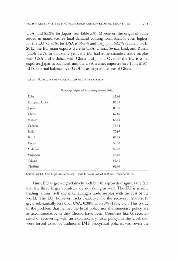
281policy alternatives for developed and developing countries
USA, and 85.3% for Japan (see Table 5.8). Moreover, the origin of value added in manufactures final demand coming from itself is even higher, for the EU 75.75%, for USA is 66.3% and for Japan 68.7% (Table 5.9). In 2015, the EU main exports were to USA, China, Switzerland, and Russia (Table 1.17). In that same year, the EU had a merchandise trade surplus with USA and a deficit with China and Japan. Overall, the EU is a net exporter, Japan is balanced, and the USA is a net importer (see Table 5.10). EU’s external balance over GDP is as high as the one of China.
table 5.8. origins of value added in gross exports
Percentage originated in exporting country (2011)
USA 85.03
European Union 85.39
Japan 85.30
China 67.89
Mexico 68.31
Canada 76.44
India 75.97
Brazil 89.28
Korea 58.37
Malaysia 59.42
Singapore 58.27
Taiwan 56.49
Thailand 61.05
Source: OECD Stat, http://stats.oecd.org, Trade In Value Added (TIVA), December 2016.
Thus, EU is growing relatively well but this growth disguises the fact that the three larger countries are not doing as well. The EU is mainly trading within itself and maintaining a trade surplus with the rest of the world. The EU, however, lacks flexibility for the recovery; 2008-2016 grew substantially less than USA, 0.38% vs 0.70% (Table 5.6). This is due to the problem that neither the fiscal policy nor the monetary policy are as accommodative as they should have been. Countries like Greece, in-stead of recovering with an expansionary fiscal policy, as the USA did, were forced to adopt traditional IMF procyclical policies, with even the
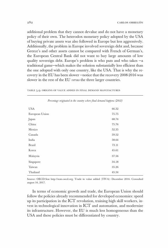
carlos obregón282
additional problem that they cannot devalue and do not have a monetary policy of their own. The heterodox monetary policy adopted by the USA of buying private assets was also followed in Europe but less aggressively. Additionally, the problem in Europe involved sovereign debt and, because Greece’s and other assets cannot be compared with French of German’s, the European Central Bank did not want to buy large amounts of low quality sovereign debt. Europe’s problem is who puts and who takes —a traditional game—which makes the solution substantially less efficient than the one adopted with only one country, like the USA. That is why the re-covery in the EU has been slower —notice that the recovery 2008-2016 was slower in the rest of the EU versus the three larger countries.
table 5.9. origins of value added in final demand manufactures
Percentage originated in the country where final demand happens (2011)
USA 66.32
European Union 75.75
Japan 68.74
China 75.76
Mexico 52.35
Canada 39.52
India 58.64
Brazil 73.11
Korea 45.61
Malaysia 37.56
Singapore 34.18
Taiwan 35.26
Thailand 45.34
Source: OECD.Stat http://stats.oecd.org. Trade in value added (TIVA): December 2016. Consulted august 16, 2017.
In terms of economic growth and trade, the European Union should follow the policies already recommended for developed economies: speed up its participation in the ICT revolution, training high skill workers, in-vest in technological innovation in ICT and automation, and modernize its infrastructure. However, the EU is much less homogeneous than the USA and these policies must be differentiated by country.
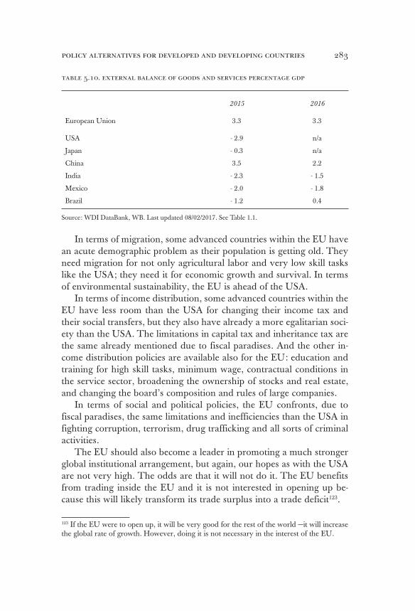
283policy alternatives for developed and developing countries
table 5.10. external balance of goods and services percentage gdp
2015 2016
European Union 3.3 3.3
USA - 2.9 n/a
Japan - 0.3 n/a
China 3.5 2.2
India - 2.3 - 1.5
Mexico - 2.0 - 1.8
Brazil - 1.2 0.4
Source: WDI DataBank, WB. Last updated 08/02/2017. See Table 1.1.
In terms of migration, some advanced countries within the EU have an acute demographic problem as their population is getting old. They need migration for not only agricultural labor and very low skill tasks like the USA; they need it for economic growth and survival. In terms of environmental sustainability, the EU is ahead of the USA.
In terms of income distribution, some advanced countries within the EU have less room than the USA for changing their income tax and their social transfers, but they also have already a more egalitarian soci-ety than the USA. The limitations in capital tax and inheritance tax are the same already mentioned due to fiscal paradises. And the other in-come distribution policies are available also for the EU: education and training for high skill tasks, minimum wage, contractual conditions in the service sector, broadening the ownership of stocks and real estate, and changing the board’s composition and rules of large companies.
In terms of social and political policies, the EU confronts, due to fiscal paradises, the same limitations and inefficiencies than the USA in fighting corruption, terrorism, drug trafficking and all sorts of criminal activities.
The EU should also become a leader in promoting a much stronger global institutional arrangement, but again, our hopes as with the USA are not very high. The odds are that it will not do it. The EU benefits from trading inside the EU and it is not interested in opening up be-cause this will likely transform its trade surplus into a trade deficit123.
123 If the EU were to open up, it will be very good for the rest of the world —it will increase the global rate of growth. However, doing it is not necessary in the interest of the EU.
carlos obregón284
Finally, in terms of the monetary and financial policy, as we men-tioned before, the EU needs to change the Euro agreement by allowing countries in problems —with significant negative external shocks— to leave temporarily the Euro Agreement and to have a floating exchange rate as well as an autonomous monetary policy. It should also enforce a truly common fiscal policy in the future and expel countries that do not comply. These policies will enhance the EU flexibility for the recovery.
Japan
Japan was the success story of the recovery years after the war. It en-tered the chips computer revolution and invented the production of cars through modules instead of the traditional lines of production used in the USA. This meant that many more car models could be produced at cheaper prices because the models share many components —produced in modules124. But, as we mentioned in chapter one, Japan was a loser with the advent of the ICT technology revolution. Japan’s economic growth has been the lowest when compared with the USA and the EU. From 1990-2016 it grew only 0.88% in per capita terms (Table 5.6). In 1986, Japan had 15.4% of global manufacture exports (Table 1.30), by 2000 it had 9.4%, and for 2015 only 5.2% (Table 1.11).
Japan entered the ICT revolution as a mature developed economy, and with its high wages it could not compete with China and other low wage countries. Its old competitive mode of production was based in local manufacturing complemented to some extent with offshore produc-tion, but the full offshore model was not in place. Therefore, Japan did not enter early the ICT revolution like a developed economy sending manufacturing production offshore.
In Table 1.5, it can be appreciated that as late as 2005 Japan’s foreign di-rect investment (FDI) outward stock as a percentage of GDP was only 8.5% as compared with 27.8% for the USA, and 34.6% for the EU —this clearly shows that Japan entered the ICT revolution too late. It has been correcting this, thus by 2015 it is already 29.7% versus 33.3% for the USA, and 59.8% for the EU. But even in 2015 a problem remains: Japan is not competitive as an offshore production center because of its high wages and it is not very interesting as place to invest and produce for local Japanese consumption– 124 Diverse car models share the same fronts, same back or same doors.
285policy alternatives for developed and developing countries
because local consumption and the service sector are not well developed. Therefore, the FDI inward stock in 2015 is only 4.1% as a percent-
age of GDP vs 30.9% for USA, and 51.3% for the EU. That means that, while in 2015 around 80 to 90% of the FDI outward stock is compensat-ed in USA and the EU by FDI inward stock, in Japan only 14% is com-pensated —this leaves the Japanese economy with less resources to grow.
Japan’s rate of economic growth, as we said, was the lowest among developed nations. As it can be seen in Table 5.6. Its GDP PPP per capita growth rate was only 0.9% in 1990-2016 vs 1.4% for the USA and 1.3% for Germany, France and the UK together. If Japan wants to increase its rate of economic growth, it would have to change substantially. It has to develop furthermore its presence in the ICT revolution by increasing even more its offshore production. For this country, it will be necessary to de-velop further the service sector to be able to absorb the unemployment that manufacturing production offshore will produce —which will be a huge cultural change for Japan. As for the rest of Japan, it has to follow the policies already mentioned for developed countries such as training high skill workers, leading technological innovations in information, communi-cations and automation. In the latter one, Japan has already a competitive advantage in relationship to the rest of the world. In the future, robot’s pro-duction will also be subject to the ICT revolution —that will accelerate with telepresence, telerobotics and virtual migration. Automation will accelerate the ICT technology. Therefore, even if Japan develops a solid competitive advantage in robotics and automation, it still needs to enter even more aggressively the ICT revolution, moving more manufacturing production offshore and developing its service sector economy.
In terms of trade, Japan’s economy is as close as the USA or the EU: merchandise trade as a percentage of GDP, in 2014-2016 was 17.7% slight-ly higher to USA 13.9% or EU 16.8% (Table 1.18). 20.2% of its exports go to USA, 17.6% to China and 11.4% to EU (Table 1.17a). It has a deficit with China and a surplus with USA and the EU (Table 1.17). The value added in exports is 85.3 and in total final demand, 86.6%; both very similar to USA and the EU (Tables 5.7 and 5.8). With the whole world, its exter-nal balance of goods and services are almost balanced versus a significant deficit for the USA and a significant surplus for the EU (Table 5.10).
One of the factors that have made the situation in Japan worse is the fact that its population is getting old, and that there has always been an anti-migration national sentiment. But without migrants and without enough offshore production, Japan is not competitive —it will have to change. It
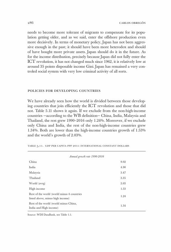
carlos obregón286
needs to become more tolerant of migrants to compensate for its popu-lation getting older, and as we said, enter the offshore production even more decisively. In terms of monetary policy, Japan has not been aggres-sive enough in the past; it should have been more heterodox and should of have bought more private assets. Japan should do it in the future. As for the income distribution, precisely because Japan did not fully enter the ICT revolution, it has not changed much since 1962, it is relatively low at around 35 points disposable income Gini. Japan has remained a very con-troled social system with very low criminal activity of all sorts.
policies for developing countries
We have already seen how the world is divided between those develop-ing countries that join efficiently the ICT revolution and those that did not. Table 5.11 shows it again. If we exclude from the non-high-income countries —according to the WB definition— China, India, Malaysia and Thailand, the rest grew 1990–2016 only 1.24%. Moreover, if we exclude only China and India, the rest of the non-high-income countries grew 1.34%. Both are lower than the high-income countries growth of 1.53% and the world’s growth of 2.03%.
table 5.11. gdp per capita ppp 2011 international constant dollars
Annual growth rate 1990-2016
China 9.02
India 4.90
Malaysia 3.47
Thailand 3.35
World (avrg) 2.03
High income 1.53
Rest of the world (world minus 4 countries listed above, minus high income)
1.24
Rest of the world (world minus China, India and High income)
1.34
Source: WDI DataBank, see Table 1.1.
287policy alternatives for developed and developing countries
Thus, due to the ICT revolution, most developing countries are not converging but diverging from the high-income economies. If these coun-tries do not develop a growth strategy, they will be even further away from the rich countries in the future. How to do it? They have to join the ICT revolution, and the Asian Development Model is a good role mod-el. They have to attract foreign direct investment and offer it privileged conditions, as long as it is directed towards exports which include value added from the recipient country. In terms of the legal framework, it must be simplified and it should be particularly transparent for the interest of the foreign investors. The developing countries have to save significantly more to be able to invest in national value-added chains, which will allow the country both to learn from the FDI and to promote economic growth. Structure must be modernized and administrative procedures simplified. Regional trade agreements should be seek when possible.
Developing countries that do not join the ICT revolution will face diffi-culties in the future. Not only because they will not grow properly, but also because they will lose an important escape valve that they had been having, that is migration. Firms in developed countries no longer need migrants; therefore, migration policies will become tougher, as we are already seeing. But if migrants are to stay in their country of origin, it means that they will need a job, and, to offer jobs, countries need to grow. For that, they need to join the ICT revolution and increase national savings. Population control policies will help but they will not be the solution if there is not sufficient economic growth. In addition to overall national economic growth, devel-oping countries must develop specific policies for those regions that were most benefited from migration in the past, and that will be hit harder by the new anti-migration policies in the developed countries.
In terms of income redistribution, developing countries must remem-ber that there is no conflict between egalitarian policies and economic growth policies. As we had been arguing, a growth strategy is compatible with many income distribution policies. It is not true that distributing income will jeopardize the growth rate of the country, but it is also not true that distributing income will increase the rate of growth. Middle mass consumption was one of the keys of capitalistic development, but that does not mean that distributing income in a developing economy trying to generate a larger middle class will stimulate economic growth. An example has been communism in diverse countries. Middle class con-sumption in a developing country, when it is associated with obsolete technology, promotes only an artificial growth that will not last. This
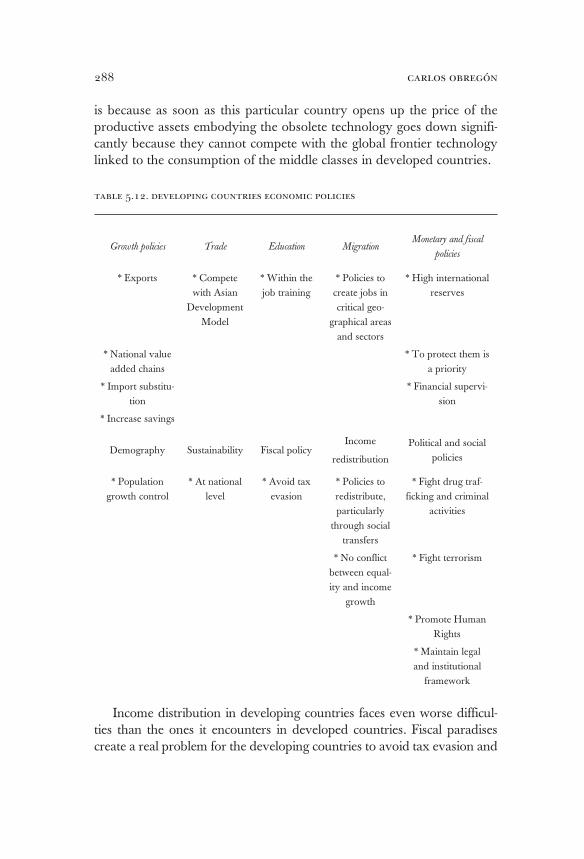
carlos obregón288
is because as soon as this particular country opens up the price of the productive assets embodying the obsolete technology goes down signifi-cantly because they cannot compete with the global frontier technology linked to the consumption of the middle classes in developed countries.
table 5.12. developing countries economic policies
Growth policies Trade Education MigrationMonetary and fiscal
policies
* Exports * Compete with Asian
Development Model
* Within the job training
* Policies to create jobs in critical geo-
graphical areas and sectors
* High international reserves
* National value added chains
* To protect them is a priority
* Import substitu-tion
* Financial supervi-sion
* Increase savings
Demography Sustainability Fiscal policyIncome
redistribution
Political and social policies
* Population growth control
* At national level
* Avoid tax evasion
* Policies to redistribute, particularly
through social transfers
* Fight drug traf-ficking and criminal
activities
* No conflict between equal-ity and income
growth
* Fight terrorism
* Promote Human Rights
* Maintain legal and institutional
framework
Income distribution in developing countries faces even worse difficul-
ties than the ones it encounters in developed countries. Fiscal paradises create a real problem for the developing countries to avoid tax evasion and
289policy alternatives for developed and developing countries
to implement a redistributive policy through capital or inheritance taxes. Therefore, they have to focus mainly in income taxes, social transfers, and education. The last two are particularly useful in developing economies. Scholarly education must be avoided. Education must be guided by the development model and be specific and worldwide competitive; On-the-job-training must be privileged. Owning stocks is less popular in develop-ing countries, which makes it more difficult to use it with redistributive purposes. Minimum wage increases, as a redistributive policy has the limi-tations that it reduces the global competiveness of the country.
Monetary and fiscal policies in developing economies cannot be coun-tercyclical because their currencies do not generate enough global trust. Thus, any significant increase in government expenditures and money supply will be met with a lower demand for the currency that will force a devaluation. And a large devaluation can cause a financial crisis in the country in question. To avoid unneeded extreme fluctuations in the cur-rency, it is advisable that developing countries maintain an austere highly disciplined monetary and fiscal policy, which should be associated with a healthy external balance, and very high international reserves are rec-ommended. Capital controls can usually be avoided through the use of the previous policies, and they should not be used —except in absolute extreme cases in which defending the international reserves must be a priority above anything else. Financial close supervision in developing economies is a must and they should start implementing a more hetero-dox monetary policy through the buying of private sector assets —this will maintain the regulators closer to the market.
Human rights, education, social transfers, and maintaining a national legal framework are important tasks in developing countries in which usually a significant portion of the population faces rough living condi-tions. The solution to these problems is even more difficult due to the existence of fiscal paradises, which difficult substantially the fight against corruption, drug trafficking and criminal activities. The developing coun-tries economic policies are presented in Table 5.12.
Mexico
As we have been saying before, Mexico is a good example that joining the ICT revolution is not enough to generate economic growth if it is
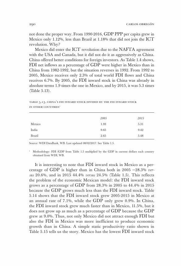
carlos obregón290
not done the proper way. From 1990-2016, GDP PPP per capita grew in Mexico only 1.12%, less than Brazil at 1.18% that did not join the ICT revolution. Why?
Mexico did enter the ICT revolution due to the NAFTA agreement with the USA and Canada, but it did not do it as aggressively as China. China offered better conditions for foreign investors. As Table 1.4 shows, FDI net inflows as a percentage of GDP were higher in Mexico than in China from 1982-1992, but the situation reverses in 1992. From 1992 to 2005, Mexico receives only 2.3% of total world FDI flows and China receives 6.7%. By 2005, the FDI inward stock in China was already in absolute terms 1.9 times the one in Mexico, and by 2015, it was 5.3 times (Table 5.13).
table 5.13. china’s fdi inward stock divided by the fdi inward stock
in other countries1
2005 2015
Mexico 1.93 5.31
India 9.65 9.42
Brazil 2.65 5.48
Source: WDI DataBank, WB. Last updated 08/02/2017. See Table 1.5.
1 Methodology: FDI /GDP from Table 1.5 multiplied by the GDP in current dollars each country obtained from WDI, WB.
It is interesting to note that FDI inward stock in Mexico as a per-centage of GDP is higher than in China both in 2005 —28.3% ver-sus 20.6%, and in 2015 44.4% versus 24.5% (Table 1.5). This reflects the problem of the economic Mexican model: the FDI inward stock grows as a percentage of GDP from 28.3% in 2005 to 44.4% in 2015 because the GDP grows much less than the FDI inward stock. Table 5.14 shows that the FDI inward stock grew 2005-2015 in Mexico at an annual rate of 7.1%, while the GDP only grew 0.9%. In China, the FDI inward stock grew much faster than in Mexico, 11.5%, but it does not grow up as much as a percentage of GDP because the GDP grew at 9.0%. Thus, not only Mexico did not attract enough FDI but also the FDI in Mexico was more inefficient to produce economic growth than in China. A simple static productivity ratio shown in Table 5.15 tells us the story. Mexico has the lowest FDI inward stock

291policy alternatives for developed and developing countries
productivity ratio of all the countries shown in both 2005 and 2015. Why? Because the Mexican economic model was not designed to pro-mote internal growth. FDI alone cannot produce adequate economic growth, internal savings are required and they were too low in the Mexican case. Table 5.16 shows saving, exports, and external balance average from 1991 to 2015 and the GDP per capita growth for China, India, Mexico, and Brazil. As it can be appreciated, both Mexico and Brazil had low savings and low economic growth.
In terms of its own GDP, Mexico is a very open economy —it even exports more than China— but because its GDP is not growing and it is becoming smaller in relationship to China in terms or world exports, Mexico has been losing competitiveness. In 1980, Mexico’s merchandise exports over the world’s were the same as China at 0.9%, in 1990 they were higher in China 1.8% vs 1.2%, but they were still close. Even as late as 2000 they were relatively close, China 3.9% vs 2.6% for Mexico. In 2001, China joined the WTO and entered fully in the ICT revolution with the Asian Development Model, the consequence is that for 2008, China’s is 8.9% vs Mexico’s 1.8%, and by 2016, China’s is 13.2% and Mexico’s is 2.3% (Table 1.8).
table 5.14. gdp growth versus fdi inward stock1. annual growth rate 2005-2015
GDP FDI GDP FDI GDP
Current dollarsInward stock cur-
rent dollarsPPP 2011
Inward stock
PPP 2011
Per capita
PPP 2011
China 17.08 19.11 9.58 11.48 9.02
Mexico 2.88 7.63 2.39 7.11 0.87
India 10.07 19.40 7.55 16.67 6.11
Brazil 7.30 10.77 2.77 6.09 1.78
Source: table 1.5 and WDI DataBank, WB updated 08/02/2017, see Table 1.1
1 Methodology: FDI/GDP from Table 1.5, GDP current dollars and GDP PPP 2011 from WDI DataBank.
The problem of Mexico its not that it does not bring value added in its exports, in fact as Table 5.8 shows, it brings the same value added than China. With the ICT revolution, the international chains of production pretty much define what is the local value added that the country could bring. Its problem is that it does not grow because a lack of savings —
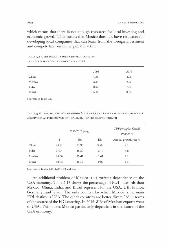
carlos obregón292
which means that there in not enough resources for local investing and economic growth. That means that Mexico does not have resources for developing local companies that can learn from the foreign investment and compete later on in the global market.
table 5.15. fdi inward stock gdp productivity
(the inverse of fdi inward stock / gdp)
2005 2015
China 4.85 4.08
Mexico 3.54 2.25
India 16.56 7.34
Brazil 5.01 3.65
Source: see Table 1.5.
table 5.16. saving, exports of goods & services and external balance of goods
& services as percentage of gdp. also, gdp per capita growth
1990-2015 (avrg)
GDP per capita. Growth
1990-2015
S Ex EB Annual growth rate %
China 44.91 23.96 3.58 9.1
India 27.94 16.30 - 2.40 4.8
Mexico 20.60 25.61 - 1.07 1.1
Brazil 19.03 11.30 - 0.27 1.4
Source: see Tables 1.28, 1.29, 1.30 and 1.6.
An additional problem of Mexico is its extreme dependence on the USA economy. Table 5.17 shows the percentage of FDI outwards than Mexico, China, India, and Brazil represent for the USA, UK, France, Germany, and Japan. The only country for which Mexico is the main FDI destiny is USA. The other countries are better diversified in terms of the source of the FDI entering. In 2016, 81% of Mexican exports went to USA. This makes Mexico particularly dependent in the future of the USA economy.
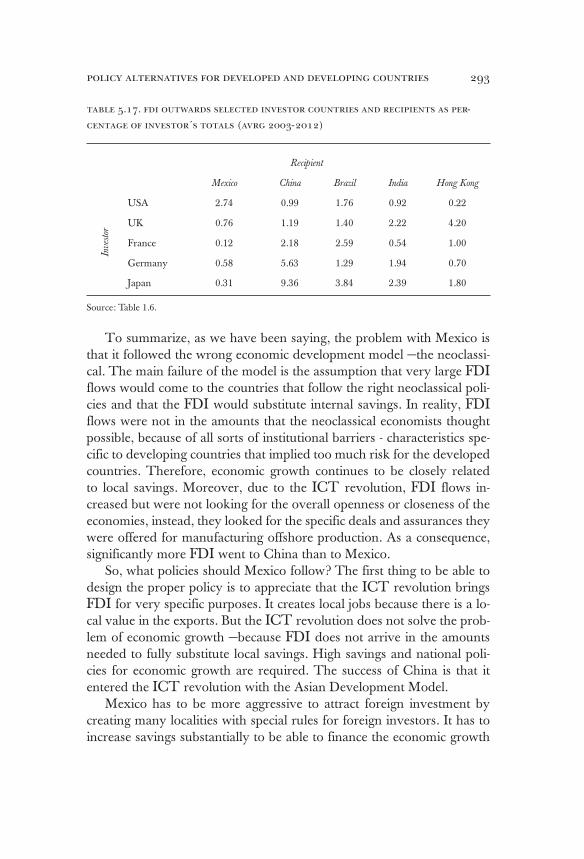
293policy alternatives for developed and developing countries
table 5.17. fdi outwards selected investor countries and recipients as per-
centage of investor´s totals (avrg 2003-2012)
Recipient
Mexico China Brazil India Hong Kong
Inve
stor
USA 2.74 0.99 1.76 0.92 0.22
UK 0.76 1.19 1.40 2.22 4.20
France 0.12 2.18 2.59 0.54 1.00
Germany 0.58 5.63 1.29 1.94 0.70
Japan 0.31 9.36 3.84 2.39 1.80
Source: Table 1.6.
To summarize, as we have been saying, the problem with Mexico is that it followed the wrong economic development model —the neoclassi-cal. The main failure of the model is the assumption that very large FDI flows would come to the countries that follow the right neoclassical poli-cies and that the FDI would substitute internal savings. In reality, FDI flows were not in the amounts that the neoclassical economists thought possible, because of all sorts of institutional barriers - characteristics spe-cific to developing countries that implied too much risk for the developed countries. Therefore, economic growth continues to be closely related to local savings. Moreover, due to the ICT revolution, FDI flows in-creased but were not looking for the overall openness or closeness of the economies, instead, they looked for the specific deals and assurances they were offered for manufacturing offshore production. As a consequence, significantly more FDI went to China than to Mexico.
So, what policies should Mexico follow? The first thing to be able to design the proper policy is to appreciate that the ICT revolution brings FDI for very specific purposes. It creates local jobs because there is a lo-cal value in the exports. But the ICT revolution does not solve the prob-lem of economic growth —because FDI does not arrive in the amounts needed to fully substitute local savings. High savings and national poli-cies for economic growth are required. The success of China is that it entered the ICT revolution with the Asian Development Model.
Mexico has to be more aggressive to attract foreign investment by creating many localities with special rules for foreign investors. It has to increase savings substantially to be able to finance the economic growth
carlos obregón294
that it requires. It must have an industrial policy of its own with the fol-lowing goals:
1. Developed national value added chains to promote local eco-nomic growth.
2. Support industries for import substitution purposes. 3. A strategy to support local companies that can become global
competitors. 4. Continue supporting companies that add value in exports.It has to modernize the NAFTA, which is a great opportunity, but
it should not depend on it for solving its economic growth problem. It should diversify as possible its sources of FDI and the countries towards which exports are directed. It has to modernize its educational system that is very scholastic today. On-the-job-training should be encouraged. The competitive model must guide education.
Mexico should continue with demographic policies aiming at slowing the population growth, but they will not be enough. Mexico is facing a serious economic growth problem which requires urgent attention. Fur-thermore, the employment problem will become even worse due to the anti-migration policies in the developed countries, particularly in USA. Therefore, in addition to the general policy for economic growth, region-al policies will ne needed for those locations that will be more negatively impacted for the reduced migration to the USA.
Income distribution in Mexico is not good, it requires to be improved, but we should not confuse the problem of income distribution with the problem of human well-being. China’s income distribution has deterio-rated but Chinese in general are, no question, much better off. The priori-ty must be economic growth and not income distribution. But as we have been saying, there is room for both. Mexico should have simultaneously three goals: economic growth, income redistribution and improving mini-mum standards of living of the marginal population.
Mexico is still awaiting a broad fiscal reform that is needed to increase savings and to promote income distribution. Monetary policy in Mexico has been traditionally, particularly lately, well managed.
In addition to economic growth, Mexico’s main problem is crime. Original drug criminals have diversified into many criminal activities and they have broken into small groups. Criminal activity corrupts and defies the political institutional life of the country and it is a serious menace for its future. This is not the topic of this book, but it had to be mentioned.

[295]
ANNEX
table 1.21. annex1
1990-2016 Year starts:
Savings Gross Savings Domestic S Gross S Domestic
World 24.45 25.16 70 66
North America 18.47 18.66 70 60
EU 21.61 22.63 75 70
Lat Am & Caribb 18.46 20.26 76 60
East Asia & Pacific 35.10 34.75 96 70
Russian Federation 27.71 31.55 94 89
Central African Republic 11.52 2.59 77 60
China 44.58 44.65 82 60
India 31.75 29.84 75 60
Source: WDI DataBank, see Table 1.1.
1 Savings are gross savings exports of goods and services and the external balance of goods and ser-vices; all presented as % of GDP. Numbers from tables 1.21 to 1.27 come from WDI DataBank and are the average of the years available at the source –which may not be the same for several countries– for the period indicated in the table (see footnote of Table 1.1). Gross savings are defined as gross national income minus total consumption plus net transfers from abroad. National income is equal to GDP plus net income received from abroad. Therefore, gross savings is the best measure of the total savings of a country. An alternative measure is domestic savings, which is defined as GDP minus total consumption, it measures the domestic effort to save; but from the point of view of economic growth, which is what interest us here, gross savings are the relevant measure. However, gross savings are available for significantly less years as shown in an annex to each one of the tables from 1.21 through 1.27. We present the comparison between both measures of savings indicating the years available per country in each case, as the reader can appreciate, the conclusions do not change.
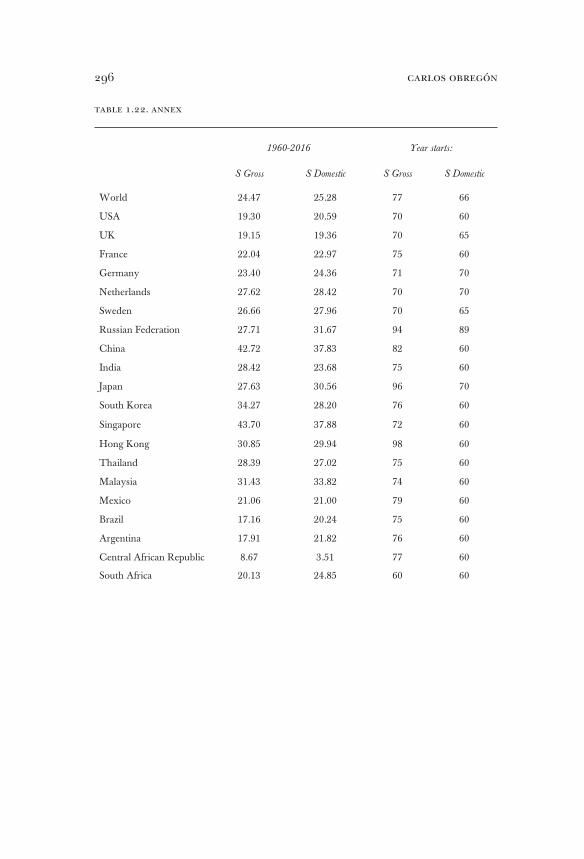
carlos obregón296
table 1.22. annex
1960-2016 Year starts:
S Gross S Domestic S Gross S Domestic
World 24.47 25.28 77 66
USA 19.30 20.59 70 60
UK 19.15 19.36 70 65
France 22.04 22.97 75 60
Germany 23.40 24.36 71 70
Netherlands 27.62 28.42 70 70
Sweden 26.66 27.96 70 65
Russian Federation 27.71 31.67 94 89
China 42.72 37.83 82 60
India 28.42 23.68 75 60
Japan 27.63 30.56 96 70
South Korea 34.27 28.20 76 60
Singapore 43.70 37.88 72 60
Hong Kong 30.85 29.94 98 60
Thailand 28.39 27.02 75 60
Malaysia 31.43 33.82 74 60
Mexico 21.06 21.00 79 60
Brazil 17.16 20.24 75 60
Argentina 17.91 21.82 76 60
Central African Republic 8.67 3.51 77 60
South Africa 20.13 24.85 60 60

297annex
table 1.22a. gdp per capita levels
Maddison Project 2013 (1990 PPP) World Bank (2011 PPP)
1950 1990 2008 1990 2016
World 2104 5149 7626 8908 15023
USA 9561 23201 31251 37062 53272
UK 6939 16430 24602 26769 38901
France 5186 17647 22047 29528 38058
Germany 3881 15929 20801 31287 44072
Netherlands 5996 17262 25112 32090 47128
Sweden 6739 17609 25181 30934 46441
USSR 2841 6894 7878 n/a n/a
Russian Federation n/a 6170 4037 20639 24026
China 448 1871 6725 1526 14401
India 619 1309 2952 1755 6093
Japan 1921 18789 22175 30447 38240
South Korea 854 8704 20454 11632 34986
Singapore 2219 14220 20454 34338 81443
Hong Kong 2218 17541 29810 26974 54279
Thailand 817 4633 8923 6651 15682
Malaysia 1559 5131 9880 10551 25660
Mexico 2365 6085 7978 12584 16831
Brazil 1672 4920 6542 10344 14023
Argentina 4987 6433 9972 10816 18479
Central African Republic 772 642 536 932 648
South Africa 2535 3834 5048 9899 12260
Source: see Table 1.1.
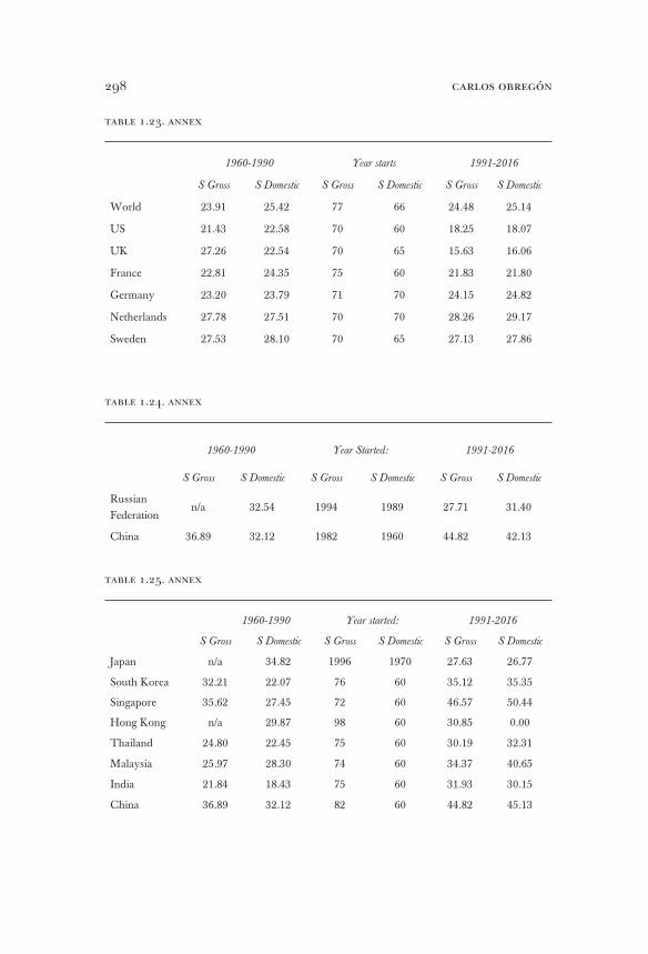
carlos obregón298
table 1.23. annex
1960-1990 Year starts 1991-2016
S Gross S Domestic S Gross S Domestic S Gross S Domestic
World 23.91 25.42 77 66 24.48 25.14
US 21.43 22.58 70 60 18.25 18.07
UK 27.26 22.54 70 65 15.63 16.06
France 22.81 24.35 75 60 21.83 21.80
Germany 23.20 23.79 71 70 24.15 24.82
Netherlands 27.78 27.51 70 70 28.26 29.17
Sweden 27.53 28.10 70 65 27.13 27.86
table 1.24. annex
1960-1990 Year Started: 1991-2016
S Gross S Domestic S Gross S Domestic S Gross S Domestic
Russian Federation
n/a 32.54 1994 1989 27.71 31.40
China 36.89 32.12 1982 1960 44.82 42.13
table 1.25. annex
1960-1990 Year started: 1991-2016
S Gross S Domestic S Gross S Domestic S Gross S Domestic
Japan n/a 34.82 1996 1970 27.63 26.77
South Korea 32.21 22.07 76 60 35.12 35.35
Singapore 35.62 27.45 72 60 46.57 50.44
Hong Kong n/a 29.87 98 60 30.85 0.00
Thailand 24.80 22.45 75 60 30.19 32.31
Malaysia 25.97 28.30 74 60 34.37 40.65
India 21.84 18.43 75 60 31.93 30.15
China 36.89 32.12 82 60 44.82 45.13
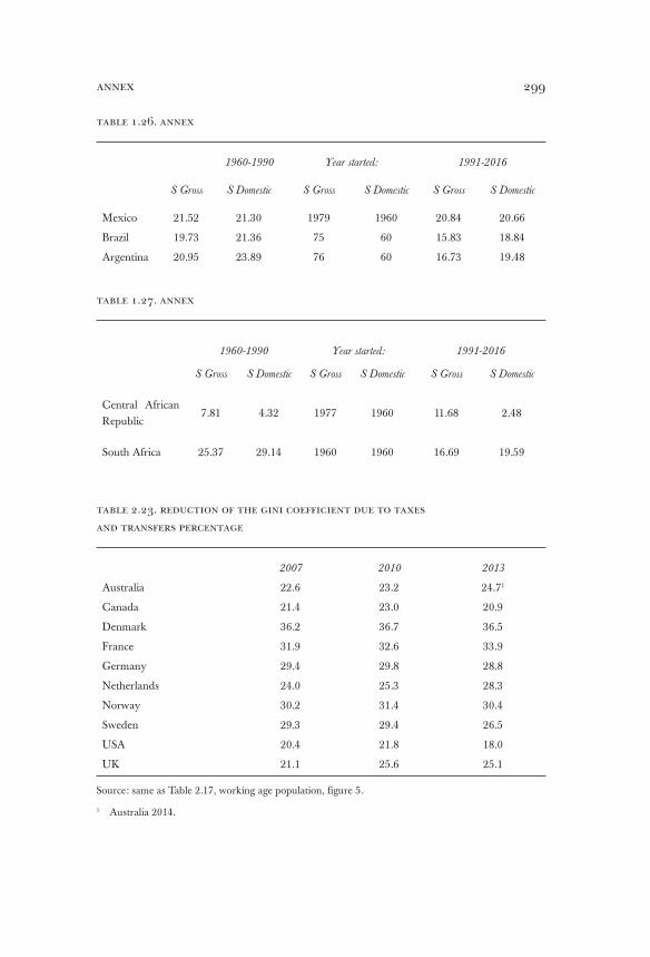
299annex
table 1.26. annex
1960-1990 Year started: 1991-2016
S Gross S Domestic S Gross S Domestic S Gross S Domestic
Mexico 21.52 21.30 1979 1960 20.84 20.66
Brazil 19.73 21.36 75 60 15.83 18.84
Argentina 20.95 23.89 76 60 16.73 19.48
table 1.27. annex
1960-1990 Year started: 1991-2016
S Gross S Domestic S Gross S Domestic S Gross S Domestic
Central African Republic
7.81 4.32 1977 1960 11.68 2.48
South Africa 25.37 29.14 1960 1960 16.69 19.59
table 2.23. reduction of the gini coefficient due to taxes
and transfers percentage
2007 2010 2013
Australia 22.6 23.2 24.71
Canada 21.4 23.0 20.9
Denmark 36.2 36.7 36.5
France 31.9 32.6 33.9
Germany 29.4 29.8 28.8
Netherlands 24.0 25.3 28.3
Norway 30.2 31.4 30.4
Sweden 29.3 29.4 26.5
USA 20.4 21.8 18.0
UK 21.1 25.6 25.1
Source: same as Table 2.17, working age population, figure 5.
1 Australia 2014.
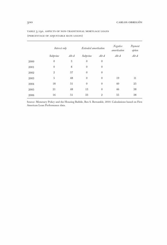
carlos obregón300
table 3.19a. aspects of non-traditional mortgage loans
(percentage of adjustable rate loans)
Interest only Extended amortization
Negative
amortization
Payment
option
Subprime Alt-A Subprime Alt-A Alt-A Alt-A
2000 0 3 0 0
2001 0 8 0 0
2002 2 37 0 0
2003 5 48 0 0 19 11
2004 18 51 0 0 40 25
2005 21 48 13 0 46 38
2006 16 51 33 2 55 38
Source: Monetary Policy and the Housing Bubble, Ben S. Bernankle, 2010. Calculations based on First American Loan Performance data.
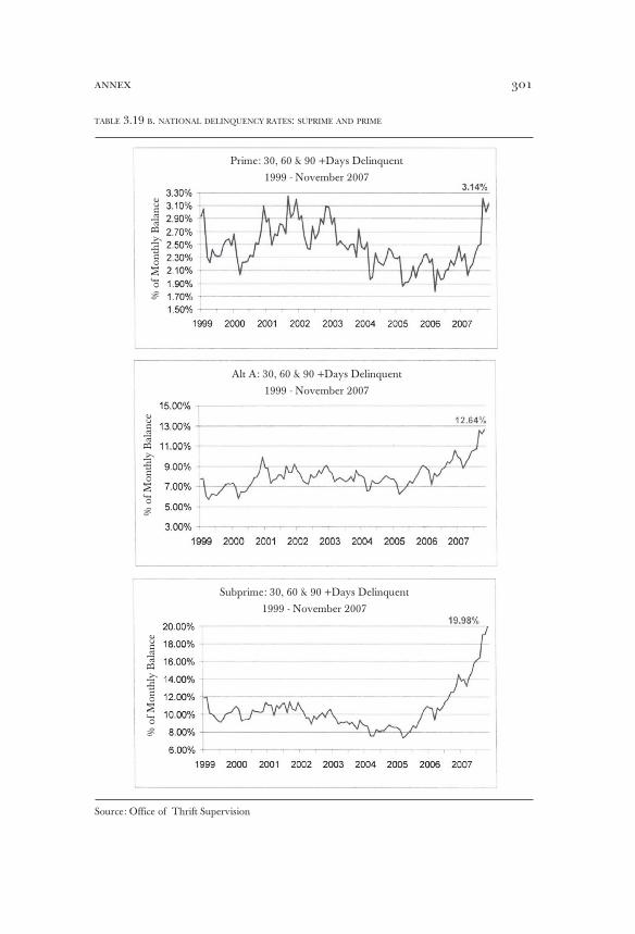
301annex
Source: Office of Thrift Supervision
TABLE 3.19 B. NATIONAL DELINQUENCY RATES: SUPRIME AND PRIME
Prime: 30, 60 & 90 +Days Delinquent
1999 - November 2007
Alt A: 30, 60 & 90 +Days Delinquent
1999 - November 2007
% o
f M
on
thly
Bal
ance
% o
f M
on
thly
Bal
ance
% o
f M
onth
ly B
alan
ce
Subprime: 30, 60 & 90 +Days Delinquent
1999 - November 2007
[302]
BIBLIOGRAPHY
Abramovitz, M. (1986). “Catching Up, Forging Ahead, and Falling Behind”. The Journal of Economic History, 46(2), 385-406. DOI: 10.1017/S0022050700046209
–––– (1993). “The Search for the Sources of Growth: Areas of Ignorance, Old and New”. The Journal of Economic History, 53(2), 217-243. DOI: 10.1017/S0022050700012882
Acemoglu, D. (1997). “Training and Innovation in an Imperfect Labour Market”. Review of Economic Studies, 64 (3), 445-464. DOI: 10.2307/2971723
Acemoglu, D., Aghion, P., & Zilibotti, F. (2002). “Distance to Frontier Selection, and Eco-nomic Growth”. NBER Working Paper 9066. DOI: 10.3386/w9066
Acemoglu, D., Johnson, S., & Robinson, J.A. (2000). The Colonial Origins of Comparative Devel-opment. MIT, unedited manuscript.
–––– (2003). “An African Success Story: Botswana”, in Rodrik, D. (Ed.). In Search of Prosperity. Analytic Narratives on Economic Growth. Princeton University Press, Princeton, 80-151.
–––– (2000a). Inefficient Redistribution. MIT, unedited manuscript. –––– (2000b). “Political Losers as a Barrier to Economic Development”. American Economic
Review, 90(2), 126-130. DOI: 10.1257/aer.90.2.126Adelman, I. (2002). “Falacies in Development Theory and Their Implications for Policy”,
in Meier, G.M., & Stiglitz, J.E. (Eds.): Frontiers of Development Economics. The Future in Perspective, Third Ed. World Bank/Oxford University Press, Washington, 103-148.
Adelman, I., & Morris, C.T. (1967). Society, Politics and Economic Development: A Quantitative Approach. Johns Hopkins University Press, Baltimore.
Adelman, I., & Robinson, S. (1978). Income Distribution Policy in Developing Countries: A Case Study of Korea. Stanford University Press, Stanford.
Adsera, A., & Debraj, R. (1998). “History and Coordination Failure”. Journal of Economic Growth, 3(3), 267-276.
Agarwala A.N. & Singh S.P. (Eds.) (1958). The Economics of Underdevelopment. Oxford Uni-versity Press, London.
Aghion, P., & Howitt, P. (1992). “A Model of Growth through Creative Destruction”. Econo-metrica, 60(2), 323-351. DOI: 0012-9682(199203)60:2<323:AMOGTC>2.0.CO;2-#
–––– (1998). Endogenous Growth Theory. MIT Press, Cambridge.–––– (2003). “Growth with Quality-Improving Innovations: An Integrated Framework”, first
treatment of a chapter of the book in press Handbook on Economic Growth, April 18, 2003.Aiyagari, S.R., Christiano, L.J., & Eichenbaum, M. (1992). “The Output, Employment, and
Interest Rate Effects of Government Consumption”. Journal of Monetary Economics, 30(1), 73-86. DOI: 10.1016/0304-3932(92)90045-4
Akerlof, G.A. (1970). “The Market for ‘Lemons’: Quality Uncertainty and the Market Mechanism”. Quarterly Journal of Economics, 84(3), 488-500. DOI: 10.2307/1879431
Akerlof, G.A., & Yellen, J.L. (1985). “A Near-Rational Model of the Business Cycle, With Wage and Price Inertia”. Quarterly Journal of Economics, 100, supplement, 823-838. DOI: 10.1093/qje/100.Supplement.823
–––– (1990). “The Fair Wage-Effort Hypothesis and Unemployment”. Quarterly Journal of Economics, 105(2), 255-283. DOI: 10.2307/2937787
Alchian, A.A. (1961). Some Economics of Property. RAND D-2316. RAND Corporation, Santa Monica (CA).
bibliography 303
–––– (1965a). “The Basis of Some Recent Advances in the Theory of Management of the Firm”. Journal of Industrial Economics, 14(1), 30-41. DOI: 10.2307/2097649
–––– (1965b). “Some Economics of Property Rights”. Il Politico, 30 (4), 816-829. –––– (1970). “Information Costs Pricing and Resource Unemployment”, in Phelps, E.S. (Dir.):
Microeconomic Foundation of Employment and Inflation Theory. W.W. Norton, New York.Alesina, A., & Drazen, A. (1991). “Why Are Stabilizations Delayed?” American Economic
Review, 81(5), 1170-1188. DOI: 10.3386/w3053Alesina, A., & Summers, L.H. (1993). “Central Bank Independence and Macroeconomic Per-
formance”. Journal of Money, Credit and Banking 25(2), 151-162. DOI: 10.2307/2077833Allen, F. Gale, D. (2007). Understanding Financial Crises. Oxford University Press, Oxford.Alt, J.R. & Martin, L.L. (1994). “Contracting and the Possibility of Multilateral Enforce-
ment”. Journal of Institutional and Theoretical Economics, 150(1), 265-271.Alt, J.R., Calvert, R., & Humes, B. (1988). “Reputation and Hegemonic Stability: A
Game Theoretic Analysis”. American Political Science Review, 82(2), 445-466. DOI: 10.2307/1957395
Amelina, M. (2000). False Transformations: From Stalin’s Peasants to Yeltsin’s Collective Farmers. World Bank, Washington, in press.
Amin, S., Faire, A., Hussein, M., & Massiah, G. (1975). La crise de l’impérialisme. Minuit, Paris.Ando, A., & Modigliani, F. (1957). “Tests of the Life-Cycle Hypothesis of Savings: Com-
ments and Suggestions”. Bulletin of the Oxford University Institute of Statistics, 19.–––– (1963): “The Life-Cycle Hypothesis of Saving: Aggregate Implications and Tests”.
American Economic Review, 53(1, part 1), 55-84.Aoki, M., Murdock, K., & Okuno-Fujiwara, M. (1997). “Beyond the East Asian Miracle:
Introducing the Market Enhancing View”, in Aoki, M., Okuno-Fujiwara, M., & Kim, H. (Eds.): The Role of Government in East Asian Economic Development: Comparative Institutional Analysis. Oxford University Press, Oxford.
Arnott, R., & Stiglitz, J.E. (1991). “Moral Hazard and Nonmarket Institution: Dysfunctional Crowding Out or Peer Monitoring?” American Economic Review, 81(1), 179-190. DOI: 10.7916/D8NV9V7F
Arrow, K.J. (1962). “The Economic Implications of Learning by Doing”. The Review of Economic Studies, 29(3), 155-173. DOI: 10.2307/2295952
–––– (1969). “The Organization of Economic Activity: Issues Pertinent to the Choice of Market versus Non-Market Allocation”, in The Analysis and Evaluation of Public Ex-penditures: The PBB-System. Joint Economic Committee, 91st Cong., 1st Sess. Vol. 1.Government Printing Office, Washington.
–––– (1988). “General Economic Theory and the Emergence of Theories of Economic Development”, in Arrow, K.J. (Ed.): The Balance between Industry and Agriculture in Economic Development. Vol. 1. Saint Martin’s Press, New York.
Arrow, K.J., & Hahn F.A. (1972). General Competitive Analysis. Holden Day, San Francisco.Arteta, C., & Wyplosz, C. (2003). “When does Capital Account Liberalization Help More
than it Hurts?” in Eichengreen, B.: Capital Flows and Crisis. MIT Press, Cambridge/London, 71-96.
Axelrod, R. (1986). The Evolution of Cooperation. Basic Books, New York.Azariadis, C. (1975). “Implicit Contracts and Underemployment Equilibria”. Journal of Po-
litical Economy, 83(6), 1183-1202. DOI: 10.1086/260388Baily, M.N. (1974). “Wages and Employment under Uncertain Demand”. The Review of
Economic Studies, 41(1), 37-50. DOI: 10.2307/2296397Bain, J. (1958). Industrial Organization. John Wiley & Sons, New York/London.Bairoch, P. & Burke, S. (Eds.) (1989). “European Trade Policy, 1815-1914”. The Cam-
bridge Economic History of Europe. Cambridge University Press, Cambridge, 1-160. DOI:10.1017/CHOL9780521225045.002
carlos obregón304
Baker, G.P., Jensen, M.C., & Murphy, K.J. (1988). “Compensation and Incentives: Practice vs. Theory”. Journal of Finance, 43(3), 593-616. DOI: 10.2307/2328185
Balassa, B. (1979). “A Stages Approach to Comparative Advantage”, in Adelman I. (Ed.): Proceedings of the Fifth World Congress of the International Economic Association. Macmillan, London, 121-156
–––– (1984). “Adjustment Policies in Developing Countries: A Reassessment”. World Devel-opment, 12 (9). World Bank, Montreal. DOI: 10.1016/0305-750X(84)90053-6
Baldwin, R. (2016). The Great Convergence. The Bellknap Press of Harvard University, Cam-bridge.
Ball, L. (1991). “The Genesis of Inflation and the Costs of Disinflation”. Journal of Money, Credit and Banking, 23(3, part 2), 453-456. DOI: 10.3386/w3621
–––– (1999). “Efficient Rules for Monetary Policy”. International Finance, 2(1), 63-83. DOI: 10.1111/1468-2362.00019
Ball, L., Mankiw, N.G., & Romer, D. (1988). “The New Keynesian Economics and the Output-Inflation Trade-off”. Brookings Papers on Economic Activity, 1, 1-65.
Ball, L., & Cecchetti, S.G. (1990). “Inflation and Uncertainty at Short and Long Horizons”. Brookings Papers on Economic Activity, 1, 215-254.
Ball, L., & Romer, D. (1990). “Real Rigidities and the Non-Neutrality of Money”. The Re-view of Economic Studies 57(2), 183-203. DOI: 10.2307/2297377
European Central Bank (January 2011). The Financial Crisis and the Strengthening of Global Policy Cooperation. Monthly bulletin.
World Bank. (2011).World Development Indicators (WDI).–––– (December 2008). Lessons from World Bank Group. Responses to Past Financial Crisis. Pre-
sented by Director-General, Evaluation.Banerjee, A., & Newman, A.F. (1998). “Information, the Dual Economy, and Develop-
ment”. Review of Economic Studies, 65(4), 631-653. DOI: 10.1111/1467-937X.00062 Baran, P.A. (1952). “On the Political Economy of Backwardness”. The Manchester School, 20,
66-84. DOI: 10.1111/j.1467-9957.1952.tb00830.x –––– (1957). The Political Economy of Growth. Modern Reader Paperbacks, New York.Barro, R.J. (1979). “On the Determination of Public Debt”. Journal of Political Economy, 87(5),
940-971. DOI: 10.1086/260807–––– (1981). “The Equilibrium Approach to Business Cycles”, in Money, Expectations and
Business Cycles. Academic Press, New York.–––– (1984). Macroeconomics. John Wiley & Sons, New York.–––– (1991). “Economic Growth in a Cross Section of Countries”. The Quarterly Journal of
Economics, 106(425), 407-443. DOI: 10.3386/w3120–––– (1997). Determinants of Economic Growth. A Cross-Country Empirical Study. MIT Press, Cam-
bridge.Barro, R.J., & Becker, G.S. (1989). “Fertility Choice in a Model of Economic Growth”. Econo-
metrica, 57(2), 481-501. DOI: 0012-9682(198903)57:2<481:FCIAMO>2.0.CO;2-F–––– (1976). “Recent Developments in Monetary Theory”. Journal of Monetary Economics,
2(2), 133-167. DOI: 10.1016/0304-3932(76)90031-3Barro, R.J., & Grossman, H.I. (1976). Money, Employment and Inflation. Cambridge University
Press, Cambridge.Barro, R.J., & Sala-i-Martin X. (2004). Economic Growth. MIT Press, Cambridge.Barsky, R., Mankiw, N.G., & Zeldes, S.P. (1986). “Ricardian Consumers with Keynesian
Propensities”. American Economic Review, 76(4), 676-691. DOI: 10.3386/w1400Barzel, Y. (1982). “Measurements Cost and the Organization of Markets”. Journal of Law
and Economics, 25(1), 27-48. DOI: 10.1086/467005 Basu, K. (2000). The Social and Political Foundations of Economics: A Prelude to Political Economy.
Oxford University Press, Oxford.

bibliography 305
Basu, S. (1995) “Intermediate Goods and Business Cycles: Implications for Productivity and Welfare”. American Economic Review, 85(3), 512-531. DOI: 10.3386/w4817
Baumol, W. (1990). “Entrepreneurship: Productive, Unproductive and Destructive”. Jour-nal of Political Economy, 98(5, part 1) 893-921. DOI: 10.1086/261712
Baxter, M., & King R.G. (1993). “Fiscal Policy in General Equilibrium”. American Economic Review, 83(3), 315-334.
Becker, G.S. (1983). “A Theory of Competition among Pressure Groups for Political Influ-ence”. Quarterly Journal of Economics, 98(3), 371-400. DOI: 10.2307/1886017
–––– (1991). “The Demand for Children”, in Becker, G.S.: A Treatise on the Family. Harvard University Press, Cambridge, chapter 5.
Becker, G.S., Murphy, K.M., & Tamura, R. (1990). “Human Capital, Fertility, and Eco-nomic Growth”. Journal of Political Economy, 98(5), S12-S37. DOI: 10.3386/w3414
Becker, G.S., & Barro, R.J. (1988). “A Reformulation of the Economic Theory of Fertility”. Quarterly Journal of Economics, CIII (412), 1-25. DOI: 10.3386/w1793
Begg, D.K.H. (1983). The Rational Expectations Revolution in Macroeconomics: Theories and Evi-dence. Johns Hopkins University Press, Baltimore.
Benetti, C. (1976). La acumulación en los países capitalistas subdesarrollados. Fondo de Cultura Económica (FCE), Mexico/Madrid/Buenos Aires.
Benhabib, J., & Farmer, R.E.A. (1999). “Indeterminacy and Sunspots in Macroeconom-ics”, in Taylor, J.B., & Woodford, M. (Eds.): Handbook of Macroeconomics, Elsevier, Amsterdam, 387-448.
Bennasy, J.P. (1982). The Economics of Market Disequilibrium. Academic Press, New York.Bernanke, B.S.–––– (1983). “Non-monetary Effects of the Financial Crisis in the Propagation of the Great
Depression”. American Economic Review, 73(3), 257-276. DOI: 10.3386/w1054–––– (1995). “The Macroeconomics of the Great Depression: A Comparative Approach”.
Journal of Money, Credit and Banking, 27(1), 1-28. DOI: 10.3386/w4814–––– (March 10, 2005). “The Global Saving Glut and the U.S. Current Account Deficit”.
Comments by Ben S. Bernanke at the Sandridge Lecture, Virginia Association of Economists, Richmond, Virginia. Bernanke presented similar comments at the Homer Jones Lecture, St. Louis, Missouri, April 14, 2005.
–––– (January 3, 2010). “Monetary Policy and the Housing Bubble” at the Annual Meeting of the American Economic Association, Atlanta, Georgia.
–––– (August 26, 2011). “The Near- and Longer-Term Prospects for the U.S. Economy” at the Federal Reserve Bank of Kansas City Economic Symposium, Jackson Hole, Wyoming.
–––– (2015). The Courage to Act. W.W. Norton & Company, New York.Bernanke, B.S., & Gertler, M. (1989). “Agency Costs, Net Worth, and Business Fluctua-
tions”. American Economic Review, 79(1), 14-31. DOI: 10.3386/w2015 Bernanke, B.S., & Lown, C.S. (1991). “The Credit Crunch”. Brookings Papers on Economic
Activity, 2, 205-247. DOI: 10.2307/2534592Bernanke, B.S., & Parkinson, M.L. (1991). “Procyclical Labor Productivity and Competing
Theories of the Business Cycle: Some Evidence from Interwar U.S. Manufacturing Industries”. Journal of Political Economy, 99(3), 439-459. DOI: 10.3386/w3503
Bernheim, B.D. (1987). “The Economic Effects of Social Security: Toward a Reconcilia-tion of Theory and Measurement”. Journal of Public Economics, 33(3), 273-304. DOI: 10.1016/0047-2727(87)90057-0
Besen, S.M., & Raskind, L.J. (1991). “An Introduction to the Law and Economics of Intel-lectual Property”. Journal of Economics Perspectives 5(1), 3-27. DOI: 10.1257/jep.5.1.3
Besley, T., & Coate, S. (1998). “Sources of Inefficiency in a Representative Democracy: A Dynamic Analysis”. American Economic Review, 88(1), 139-156.

carlos obregón306
Bhagwati, J. (1985). Essays of Development Economics. Vol. 1. MIT Press, Cambridge.–––– (1998). “The Capital Myth. The Difference between Trade in Widgets and Trade in
Dollars”. Foreign Affairs, 77(3), 7-12. DOI: 10.2307/20048871 Bank of International Settlements (BIS). Quarterly Review, September 2011.Black, F. (1982). “General Equilibrium and Business Cycles”. NBER Working Paper 950.
DOI: 10.3386/w0950 Blanchard, O.J., & Diamond, P.A. (1989). “The Beveridge Curve”. Brookings Papers on Eco-
nomic Activity, 1, 1-76.Blanchard, O.J., & Fischer, S. (1989). Lectures on Macroeconomics. MIT Press, Cambridge.Blanchard, O.J., & Kiyotaki, N. (1987). “Monopolistic Competition and the Effects of Ag-
gregate Demand”. American Economic Review, 77(4), 647-666. DOI: 10.3386/w1770Blanchard, O.J., & Summers, L.H. (1986). “Hysteresis and the European Unemployment
Program”. NBER Macroeconomics Annual, 1, 15-78. DOI: 10.3386/w1950 Blanchard, O.J., & Wolfers, J. (1999). “The Role of Shocks and Institution in the Rise of
European Unemployment”. NBER Working Paper 7282. DOI: 10.3386/w7282 Blaug, M. (1978). Economic Theory in Retrospect. Third Ed. Cambridge University Press, Cambridge.Blinder, A.S. Offshoring: The Next Industrial Revolution? Foreign Affairs March/April 2016
issue.Bloom, D.E., & Sachs, J.D. (1998). “Geography, Demography, and Economic Growth in
Africa”. Brookings Papers on Economic Activity (2), 207-295. DOI: 10.2307/2534695 Blyth, M. (2003). Great Transformations. Economic Ideas, and Institutional Change in the Twentieth
Century. Cambridge University Press, Cambridge.Bordo, M.D. (May 1981). “The Classical Gold Standard; Some Lessons for Today”. Fed-
eral Reserve Bank of St. Louis.–––– (1998). “The Financial Crisis of 1825 and the Restructuring of the British Financial
System”, commentary. Review, 80(3), 77-82, Federal Reserve Bank of St. Louis.Bordo, M.D., Dueker, M., Wheelock, D. (2001). “Aggregate Price Shocks and Financial
Stability: the United Kingdom 1796-1999”. Working Papers 2001-018A, Federal Reserve Bank of St. Louis.
Boulding, K. E.–––– (1952). “Welfare Economics” in Bob Haley (Ed.): A Survey of Contemporary Economics.
Vol. II. The American Economic Association, Homewood (IL).–––– (1957). “A New Look at Institutionalism”. The American Economic Review, papers and
proceedings, 47(2), 1-12.–––– (1971). The Image. University of Michigan Press, Ann Arbor.–––– (1982). Evolutionary Economics. Second Ed. Sage Publications, Beverly Hills/London.Bourguignon, F. (2015). The Globalization of Inequality. Princeton University Press, Princeton.Bourguignon, F. & Morrison, C. (2002). “Inequality among World Citizens 1820-1992”.
American Economic Review, 92 (4), 727-744. DOI: 10.1257/00028280260344443Boyd, R., & Richerson P.J. (1985). Culture and the Evolutionary Process. University of Chicago
Press, Chicago.Branson, W.H. (1997). Macroeconomic, Theory and Policy. Third Ed. Harper & Row, New York.Braun, R.A. (1994). “Tax Disturbances and Real Economic Activity in the Postwar
United States”. Journal of Monetary Economics, 33(3), 441-462. DOI: 10.1016/0304-3932(94)90039-6
Bresciani-Turroni, C. (1937). The Economics of Inflation: A Study of Currency, Depreciation in Post-war Germany. Allen & Unwin, London.
Brownlee, O.H., & Buttrick, J.A. (1968). Producer, Consumer, and Social Choice. McGraw-Hill, New York.
Bruno, M., & Chenery, H.B. (1962). “Development Alternatives in an Open Economy”. Economic Journal, 72(285), 79-103. DOI: 10.2307/2228618
bibliography 307
Bruno, M., & Easterly, W. (1998). “Inflation Crises and Long Run Growth”. Journal of Monetary Economics 41(1), 3-26. DOI: 10.1016/S0304-3932(97)00063-9
Bruno, M., & Sachs, J.E. (1985). Economics of Worldwide Stagflation. Harvard University Press, Cambridge.
Buchanan J.M., & Wagner, R.E. (1977). Democracy in Deficit. Academic Press, New York.Buchanan, J.M. (1986). Liberty, Market, and the State. Wheatsheaf Books, Brighton.Buiter, W.H., & Sibert, A.C. (1999). “UDROP: A Small Contribution to the New Interna-
tional Financial Architecture”. International Finance, 2, 227-248. DOI: 10.1111/1468-2362.00026
Burmeister, E., Dobell, R., & Kuga, K. (1968). “A Note on the Global Stability of a Simple Growth Model with Many Capital Goods”. Quarterly Journal of Economics, 82(4), 657-665. DOI: 10.2307/1879605
Burnside, C., Eichenbaum, M., & Rebelo, S. (1999). “Prospective Deficits and the Asian Currency Crisis”. Policy Research Working Paper Series 2174, World Bank.
–––– (2000). “Understanding the Korean and Thai Currency Crises”. Economic Perspectives, issue Q III, Federal Reserve Bank of Chicago, 45-60.
–––– (2001). “Hedging and Financial Fragility in Fixed Exchange Rate Regimes”. European Economic Review, 45(7), 1151-1193. DOI: 10.3386/w7143
Caballero, R.J. (1999). “Aggregate Investment” in Taylor, J.B., & Woodford, M. (Eds.): Handbook on Macroeconomics, 813-862. DOI: 10.1016/S1574-0048(99)10020-X
–––– (2000). Macroeconomic Volatility in Latin America: A View and Three Case Studies. Mimeo, MIT, Cambridge.
Caballero, R.J., & Krishnamurthy, A. (2001). “Smoothing Sudden Stops”. NBER Working Papers 8427. DOI: 10.3386/w8427
Cagan, P. (1956). “The Monetary Dynamics of Hyperinflation” in Friedman, M. (Ed.): Studies in the Quantity Theory of Money. University of Chicago Press, Chicago, 25-117.
Calomiris, C., & Meltzer, A. (1999). Reforming the IMF. Mimeo, Columbia Business School/Carnegie Mellon University.
Calvert, R.L. (1987). “The Rational Choice Theory of Social Institutions: Cooperation, Coor-dination, and Communication” in J.S. Banks & E.A. Hanushek (Eds.): Modern Political Economy: Old Topics, New Directions. Cambridge University Press, Cambridge, 216-269.
–––– (1995). “Rational Actors, Equilibrium, and Social Institutions”, in J. Knight, & Sened, I. (Eds.): Explaining Social Institutions. University of Michigan Press, Ann Arbor, 57-93.
Calvo, G. (1988). “Servicing the Public Debt: The Role of Expectations”. American Economic Review, 78(4), 647-661. DOI: 10.1016/B978-0-444-87387-3.50017-7
Campbell, J.Y. (1994). “Inspecting the Mechanism: An Analytical Approach to the Sto-chastic Growth Model”. Journal of Monetary Economics 33(3), 463-506. DOI: 10.1016/0304-3932(94)90040-X
Campbell, J.Y., & Cochrane, J.H. (1999). “By Force of Habit: A Consumption-Based Ex-planation of Aggregate Stock Market Behavior”. Journal of Political Economy 107(2), 205-251. DOI: 10.1086/250059
Campbell, J.Y., & Mankiw, N.G. (1987). “Are Output Fluctuations Transitory?” Quarterly Journal of Economics, 102, 857-880. DOI: 10.3386/w1916
–––– (1989a). “International Evidence on the Persistence of Economic Fluctuations”. Jour-nal of Monetary Economics, 23(2), 319-333. DOI: 10.1016/0304-3932(89)90054-8
–––– (1989b). “Consumption, Income and Interest Rates: Reinterpreting the Time Series Evidence”. NBER Macroeconomics Annual, 4, 185-216. DOI: 10.3386/w2924
Campos, N.F., & Nugent, J.B. (1999). “Development Performance and the Institutions of Governance: Evidence from East Asia and Latin America”. World Development, 27(3), 439-452. DOI: 10.1016/S0305-750X (98)00149-1
carlos obregón308
Caplin, A.S., & Spulber, D.F. (1987). “Menu Costs and the Neutrality of Money”. Quarterly Journal of Economics, 102, 703-725. DOI: 10.3386/w2311
Cardoso, E., & Helwege, A. (1992). Latin America’s Economy. Diversity, Trends and Conflicts. MIT Press, Cambridge.
Carlton, D.W. (1982). “The Disruptive Effects of Inflations on the Organization of Markets”, in Hall, R.E. (Ed.): Inflation: Causes and Effects. University of Chicago Press, Chicago, 139-152.
Carroll, C.D. (1992). “The Buffer-Stock Theory of Saving: Some Macroeconomic Evi-dence”. Brookings Papers on Economic Activity, (2), 61-156. DOI: 10.2307/2534582
–––– (1997). “Buffer-Stock Saving and the Life Cycle/Permanent Income Hypothesis”. Quarterly Journal of Economics, 112(1), 1-55. DOI: 10.1162/003355397555109
Carroll, C.D., & Summers, L.H. (1991). “Consumption Growth Parallels Income Growth: Some New Evidence” in Bernheim, B.D., & Shoven, J.B. (Eds.): National Saving and Economic Performance. Chicago University Press, Chicago.
Caruana Jaime-Director of Bank for International Settlements. (2010). “Financial stability: 10 questions and about seven answers”, speech at the 50th Anniversary Symposium of the Reserve Bank of Australia, February. https://www.bis.org/speeches/sp100209.pdf
Caselli, F., & Coleman, W.J. (2001). “Cross-Country Technology Diffusion: The Case of Computers”. American Economic Review, 91(2), 328-335. DOI: 10.3386/w8130
Cass, D., & Shell, K. (1983). “Do Sunspots Matter?” Journal of Political Economy, 91(2), 193-227. DOI: 10.1086/261139
Chang, R., & Velasco, A. (1999). “Liquidity Crises in Emerging Markets: Theory and Pol-icy” in Bernanke, B., & Rotemberg, J. (Eds.): NBER Macroeconomics Annual. MIT Press, Cambridge.
Chapela, L., & Obregon, C. (1980). “El valor de la teoría del valor” in Leff, E. (Ed.): Teoría del valor. National Autonomous University of Mexico (UNAM), Mexico, 173-210.
Chenery, H. (1955). “The Role of Industrialization in Development Programs”. American Economic Review, 45(2), 40-57.
Chenery, H.B. (1960). “Patterns of Industrial Growth”. American Economic Review, 50(4), 624-654.–––– (1975). “Restructuring the World Economy”. Foreign Affairs, 53(2), 242-263. DOI:
10.2307/20039506 Chenery, H.B., & Srinivasan, T.N. (Eds.) (1988). Handbook of Development Economics. Vol. 1.
North-Holland, Amsterdam.Chenery, H.B., & Syrquin, M. (1975). Patterns of Development, 1950-1970. Oxford University
Press, London.Chomsisengphet, S, Penningto-Crooss, A. (January-February 2006). “The Evolution of the
Subprime Mortgage Market”. Federal Reserve Bank of St Louis. Christiano, L.J., & Eichenbaum, M. (1992). “Current Real-Business-Cycle Theories and
Aggregate Labor-Market Fluctuations”. American Economic Review, 82(3), 430-450.Clark, C.W. (1977). “The Economics of Overexploitation” in Hardin, G., & Baden, J.
(Eds.): Managing the Commons. Freeman, San Francisco, 82-95.Clark, G., & Wolcott, S. (2003). “One Polity, Many Countries: Economic Growth in India,
1873-2000” in Rodrik, D. (Ed.): In Search of Prosperity. Analytic Narratives on Economic Growth. Princeton University Press, Princeton, 53-79.
Clower, R.W. (1967). “A Reconsideration of the Microfoundations of Monetary Theory”. Economic Inquiry, 6(1), 1-8. DOI: 10.1111/j.1465-7295.1967.tb01171.x
Clower, R.W., & Leijonhufvud, A. (1975). “The Coordination of Economic Activities: A Keynesian Perspective”. American Economic Review Papers and Proceedings, 65(2), 182-188.
Coase, R.H. (1937). “The Nature of the Firm”. Economica, 4(16), 386-405. Reprinted in Stigler, G.J., & Boulding, K.E. (Eds.): Readings in Price Theory (1952). Richard D. Irwin, Homewood.
–––– (1960). “The Problem of Social Cost”. Journal of Law and Economics, 3, 1-44.
bibliography 309
–––– (1972). “Industrial Organization: A Proposal for Research” in Fuchs, V.R. (Ed.): Policy Issues and Research Opportunities in Industrial Organization. NBER, New York, 59-73.
–––– (1978). “Economics and Contiguous Disciplines”. Journal of Legal Studies, 7(2), 201-211. DOI: 10.1086/467590
–––– (1984). “The New Institutional Economics”. Journal of Institutional and Theoretical Eco-nomics, 140, 229-231.
Cogley, T., & Nason, J.M. (1995). “Output Dynamics in Real-Business-Cycle Models”. American Economic Review, 85(3), 492-511.
Cole, H., & Kehoe, T. (1998). A Self-fulfilling Debt Crisis. Federal Reserve of Minneapolis Staff Report 211.
Coleman, J.S. (1990). Foundations of Social Theory. Belknap Press/Harvard University Press, Cambridge.
Collier, P. (1998). “Social Capital and Poverty”. Social Capital Initiative Working Paper 4, World Bank, Washington.
Cook, T., & Hahn, T. (1989). “The Effect of Changes in the Federal Funds Rate Target on Market Interest Rates in the 1970s”. Journal of Monetary Economics, 24(3), 331-351. DOI: 10.1016/0304-3932(89)90025-1
Cooper, R. (1984). “A Monetary System for the Future”. Foreign Affairs, 63(1), 166-184. DOI: 10.2307/20042091
Cooper, R., Dornbusch, R. & Hall, R. (1982). “The Gold Standard: Historical Facts and Future Prospects”. Brookings Papers on Economic Activity, 13(1), 1-56. DOI: 10.2307/2534316
Cooter, R.D. (2000). “Law from Order: Economic Development and the Jurisprudence of Social Norms” in Olson, M., & Käh-könen, S. (Eds.): A Not-So-Dismal Science. Oxford University Press, Oxford, 228-244.
Corsetti, G., Presenti, P., & Roubini, N. (1999). What Caused the Asian Currency and Financial Crisis? Part I: A Macroeconomic Overview, mimeo.
Craine, R. (1989). “Risky Business: The Allocation of Capital”. Journal of Monetary Economics, 23(2), 201-218. DOI: 10.1016/0304-3932(89)90048-2
Cukierman, A., Kalaitzidakis, P., Summers, L.H., & Webb, S.B. (1993). “Central Bank Independence, Growth, Investment, and Real Rates”. Carnegie-Rochester Conference Series on Public Policy, 39, 95-140. DOI: 10.1016/0167-2231(93)90005-H
Cukierman, A., Webb, S.B., & Neyapti, B. (1992). “Measuring the Independence of Central Banks and its Effect on Policy Outcomes”. World Bank Economic Review, 6(3), 353-398. DOI: 10.1093/wber/6.3.353
Cukierman, A., & Meltzer, A.H. (1986). “A Theory of Ambiguity, Credibility and Inflation under Discretion and Asymmetric Information”. Econometrica, 54(5), 1099-1128. DOI: 10.2307/1912324
Dahlman, C.J. (1979). “The Problem of Externality”. Journal of Law and Economics, 22(1), 141-162. DOI: 10.1086/466936
Damasio, A. (2010). Self Comes to Mind. Random House. New York. Davidson, P. (1978). Money and the Real World. Second Ed. Macmillan, London.Davis, M., Lehnert, A. & Martin, R. (December 2007). “The Rent Price Ratio for the Ag-
gregate Stock of Owner Occupied Housing”. Web.Davis, S.J., & Haltiwanger, J. (1999). “On the Driving Forces behind Cyclical Movements
in Employment and Job Reallocation”. American Economic Review, 89(5), 1234-1258. DOI: 10.3386/w5775
De Alessi, L. (1983). “Property Rights, Transaction Costs, and X-efficiency”. American Eco-nomic Review, 73(1), 64-81.
De Long, J.B., & Shleifer, A. (1993). “Princes and Merchants: European City Growth be-fore the Industrial Revolution”. Journal of Law and Economics, 36(2), 671-702. DOI: 10.1086/467294
carlos obregón310
De Melo, M., Denizer, C., & Gelb, A. (1996). “Patterns of Transition from Plan to Mar-ket”, World Bank Economic Review, 10(3), September 1996, 397-424. DOI: 10.1093/wber/10.3.397
De Soto, H. (2000). The Mystery of Capital. Why Capitalism Triumphs in the West, and Fails Every-where Else. Basic Books, New York.
Deaton, A.S. (1998). The Analysis of Household Surveys: A Microeconometric Approach to Develop-ment Policy. Johns Hopkins University Press/World Bank, Baltimore.
Debelle, G. (1996). “The Ends of Three Small Inflations: Australia, New Zealand, and Canada”. Canadian Public Policy, 22(1), 56-78. DOI: 10.2307/3551749
Demsetz, H. (1964). “The Exchange and Enforcement of Property Rights”. Journal of Law and Economics, 7, 11-26. DOI: 10.1086/466596
–––– (1967). “Toward a Theory of Property Rights”. American Economic Review, papers and proceedings, 57(2), 347-359.
–––– (1969). “Information and Efficiency: Another Viewpoint”. Journal of Law and Economics, 12(1), 1-22. DOI: 10.1086/466657
Démurger, S. (2001). “Infrastructure Development and Economic Growth: An Explanation for Regional Disparities in China”. Journal of Comparative Economics, 29(1), 95-117. DOI: 10.1006/jcec.2000.1693
Diamond, P.A. (1982). “Aggregate Demand Management in Search Equilibrium”. Journal of Political Economy 90(5), 881-894. DOI: 10.1086/261099
Diamond, D., Dybvig, P. (1983). “Bank Runs, Deposit Insurance, and Liquidity”. Journal of Political Economy, 91(3), 401-419. DOI: 10.1086/261155
Dixit, A.K. (1996). The Making of Economic Policy: A Transaction Cost Politics Perspective. MIT Press, Cambridge.
Dobb, M. (1966). Soviet Economic Development since 1917. Routledge, New York/London.–––– (1975). Theories of Value and Distribution since Adam Smith. Cambridge University Press,
Cambridge.Domar, E. (1947). “Expansion and Employment”. American Economic Review, 37(1), 34-55.Dornbusch, R. (1976a). “Expectations and Exchange Rate Dynamics”. Journal of Political
Economy, 84(6), 1161-1176. DOI: 10.1086/260506 –––– (1976b). “Exchange Rate Expectations and Monetary Policy”. Journal of International
Economics, 6(3), 231-244. DOI: 10.1016/0022-1996(76)90001-5Dos Santos, T. (1969). “La crisis de la teoría del desarrollo y las relaciones de dependencia
en América Latina”, in Jaguaribe, H., et al. (Eds.): La dependencia político-económica de América Latina. Centro de Estudios Socio-Económicos (CESO) Bulletin, Universi-dad de Chile, 3, Chile.
Dowrick, S., & Nguyen, D. (1989). “OECD Comparative Economic Growth 1950-1985: Catch-Up and Convergence”. American Economic Review, 79(5), 1010-1030.
Easterlin, R. (1999). “How Beneficent is the Market? A Look at the Modern History of Mortality”. European Review of Economic History, 3(3), 257-294. DOI: 10.1017/S1361491699000131
Easterly, W. (1993). “How Much Do Distortion Affect Growth?” Journal of Monetary Eco-nomics, 32(2), 187-212. DOI: 10.1016/0304-3932(93)90002-W
–––– (2003). National Policies and Economic Growth: A Reappraisal. New York University, New York.
Easterly, W., & Levine, R. (1997). “Africa’s Growth Tragedy: Policies and Ethnic Divisions”. Quarterly Journal of Economics, 112(4), 1203-1250. DOI: 10.1162/003355300555466
Eatwell, J., & Taylor, L. (Eds.) (1999). Global Finance at Risk: The Case for International Regula-tion. In press.
–––– (Eds.) (2002). International Capital Markets: Systems in Transition. Oxford University Press, New York.
bibliography 311
U.S. Government. Economic Report of the President 2007, 2008, 2009, 2010, 2011. United States Government Printing Office (GPO).
Eichengreen, B. (1999a). Toward a New International Financial Architecture: A Practical PostAsia Agenda. Institute for International Economics, Washington.
–––– (1999b). “Bailing in the Private Sector” in Hunter, W., Kaufman, G., & Krueger, T. (Eds.). The Asian Financial Crisis: Origins, Implications and Solutions. Kluwer Academic Publishers, New York.
–––– (2002). Financial Crises and What to do About Them. Oxford University Press, Oxford.–––– (2003). Capital Flows and Crises. MIT Press, Cambridge.Eichengreen, B., & Bordo, M. (2001). Crises Now and Then: What Lessons from the Last Era of
Financial Globalization? University of California, Berkeley.Eichengreen, B., & Portes, R. (1989). “Dealing with Debt: The 1930s and the 1980s”. Econom-
ics Working Papers, University of California, Berkeley, 89-104. DOI: 10.3386/w2867–––– (1990). “The Interwar Debt Crisis and Its Aftermath”. World Bank Research Observer,
5-1, Oxford University Press, January 1990, 69-94. DOI: 10.1093/wbro/5.1.69 –––– (1997). “Managing Financial Crises in Emerging Markets”. Proceedings, Federal Re-
serve Bank of Kansas City, 193-225. DOI: 10.2469/dig.v28.n4.355Emmanuel, A. (1972). Unequal Exchange: A Study of the Imperialism of Trade. Monthly Review
Press, New York/London.Engerman, S.L., Haber, S., & Sokoloff, K.L. (1999). Inequality, Institutions, and Differential
Paths of Growth among New World Economies. University of California, Department of Economics, Los Angeles, processed.
Engerman, S.L., & Sokoloff, K.L. (1997). “Factor Endowments, Institutions, and Differ-ential Paths of Growth Among New World Economies: A View From Economic Historians of the United States” in Haber, S. (Ed.): How Latin America Fell Behind: Essays on the Economic Histories of Brazil and Mexico, 1800-1914. Stanford University Press, Stanford, 260-304.
Escobar, A. (1995). Encountering Development. The Making, and Unmaking of the Third World. Princeton University Press, Princeton.
Evans, I. (1997). Bureaucracy and Race: Native Administration in South Africa. University of Cali-fornia Press, Berkeley.
Fama, E.F. (1970). “Efficient Capital Markets: A Review of Theory and Empirical Work”. Journal of Finance, 25(2), 383-417. DOI: 10.2307/2325486
Fama, E.F., & Jensen, M. (1983). “Separation of Ownership and Control”. Journal of Law and Economics, 26(2), 301-325. DOI: 10.1086/467037
Fazzari, S.M., Hubbard, R.G., & Petersen, B.C. (1988). “Financing Constraints and Cor-porate Investment”. Brookings Papers on Economic Activity, 1, Washington, 141-206. DOI: 10.2307/2534426
Feldstein, M.S.–––– (1977). “Social Security and Private Savings: International Evidence in an Extended
Life-Cycle Model” in The Economics of Public Services, An International Economic Associa-tion Conference Volume. Harvard University Press, Boston.
–––– (1998a). “Refocusing the IMF”. Foreign Affairs, 77(2), 20-33. DOI: 10.2307/20048786–––– (1998b). “What the IMF Should Do” Wall Street Journal. New York, October 6, 1998.–––– (1999). “Self-Protection for Emerging Market Economies”. NBER Working Papers
6907. DOI: 10.3386/w6907Fernandez R., & Rodrik, D. (1991). “Resistance to Reform: Status Quo Bias in the Presence
of Individual-Specific Uncertainty”. American Economic Review, 81(5), 1146-1155.Ferrero, A. (2011). “House Price Booms and Current Account Deficits”. Federal Reserve
Bank of New York, February. FHFA, July 2010. Housing and Mortgage Markets in 2010.
carlos obregón312
––––, June 2011 report.Financial Services Authority of England (FSA), spring 2009. Turner Report. Web.Fischer, S. (1977). “Long-Term Contracts, Rational Expectations and the Optimal Money
Supply Rule”. Journal of Political Economy, 85, 191-205. DOI: 10.1086/260551–––– (1980). “On Activist Monetary Policy with Rational Expectations” in Fischer, S.
(Dir.): Rational Expectations and Economic Policy. University of Chicago Press, Chicago.–––– (1993). “The Role of Macroeconomic Factors in Growth”. Journal of Monetary Econom-
ics, 32, 485-512.–––– (1999). Reforming the International Financial System. Mimeo, IMF.–––– (2000). “On the Need for an International Lender of Last Resort”. Journal of Economic
Perspectives, 13(4), 85-104.Fishlow, A. (1991). “Some Reflections on Comparative Latin American Economic Per-
formance and Policy” in Banuri, T. (Ed.): Economic Liberalization: No Panacea— The Experiences of Latin America and Asia. Oxford University Press, Oxford.
Foley, D.K. (1970). “Economic Equilibrium with Costly Marketing”. Journal of Economic Theory, 2(3), 276-291. DOI: 10.1016/0022-0531(70)90042-6
Frank, A.G. (1967). Capitalism and Underdevelopment in Latin America. Historical Studies of Chile and Brazil. Monthly Review Press, New York.
Frank, R.H. (1992). “Melding Sociology and Economics: James Coleman’s Foundations of Social Theory”. Journal of Economic Literature, 30, 147-170.
Freddie Mac Update, September 2011. Web.Friedman, M. (1968). “The Role of Monetary Policy”. American Economic Review, 58, 1-17.–––– (Dir.) (1956). Studies in the Quantity Theory of Money. University of Chicago Press, Chicago.Friedman, M., & Schwartz, A.J. (1963). “Money and Business Cycles”. Review of Economics
and Statistics, 45 February 1963, 32-64. Reprinted in Friedman, M., & Schwartz, A.J.: Monetary Trends in the United States and the United Kingdom: Their Relationship to Income, Prices and Interest Rates, 1867-1982. University of Chicago Press, Chicago, 1982.
Fuhrer, J.C. (1997). “The (Un)Importance of Forward-Looking Behavior in Price Specifica-tions”. Journal of Money, Credit and Banking 29(3), 338-350. DOI: 10.2307/2953698
Furtado, C. (1963). The Economic Growth of Brazil. University of California Press, Berkeley.–––– (1976). Economic Development of Latin America. Second Ed. Cambridge University Press,
Cambridge/London/New York/ Melbourne.Furubotn, E.G., & Richter, R. (2003). Institutions and Economic Theory. The Contribution of the
New Institutional Economics. University of Michigan Press, Ann Arbor.Gaertner, W., Pattanaik, P.K., & Suzumura, K. (1992). “Individual Rights Revisited”. Eco-
nomica, 59(234), 161-177. DOI: 10.2307/2554744Gallup, J.L., Sachs, J., & Mellinger, A. (1999). “Geography and Economic Growth” in Ples-
kovic, B., & Stiglitz, J.E. (Eds.): Annual World Bank Conference on Development Economics 1998. World Bank, Washington, 127-178.
Gandolfo, G. (1983). Economic Dynamics: Methods, and Models. Revised Ed. North-Holland, Amsterdam.
Gardenfors, P. (1981). “Rights, Games and Social Choice”. Noûs, 15(3), 341-356. DOI: 10.2307/2215437
Garrett, G., & Weingast, B.R. (1993). “Ideas, Interests, and Institutions: Constructing the European Community’s Internal Market” in Goldshein, J., & Keohane, R. (Eds.): Ideas and Foreign Policy. Cornell University Press, New York, 173-206.
Gerschenkron, A. (1962). Economic Backwardness in Historical Perspective. Belknap Press/Har-vard University Press, Cambridge.
Gertler, M., & Gilchrist, S. (1994). “Monetary Policy, Business Cycles and the Behavior of Small Manufacturing Firms”. Quarterly Journal of Economics, 109(2), 309-340. DOI: 10.2307/2118465
bibliography 313
Ghosh, A.R. (1995). “Intertemporal Tax-Soothing and the Government Budget Surplus: Canada and the United States”. Journal of Money, Credit and Banking, 27, part 1, 1033-1045.
Giavazzi, F., & Pagano, M. (1990). “Can Severe Fiscal Contractions Be Expansionary? Tales of Two Small European Countries”. NBER Macroeconomics Annual, 5, 75-111. DOI: 10.3386/w3372
Giddens, A. (1998). The Third Way and the Renewal of Social Democracy. Polity, Cambridge.Gilson, R. (1984). “Value Creation by Business Lawyers: Legal Skills and Asset Pricing”.
Law and Economics Program Working Paper 18, Stanford University, Stanford.Glaeser, E.; Gottlieb, D.; Gyourko. (July 28, 2010). “Can Cheap Credit Explain The Hous-
ing Boom?” Web, Harvard, Cambridge.Goldin C. & Katz, L. (2010). The Race between Education and Technology. The Bellknap Press of
Harvard University, Cambridge Massachusetts.Goolsbee, A. (1998). “Investment Tax Incentives, Prices, and the Supply of Capital Goods”.
Quarterly Journal of Economics, 113, 121-148. DOI: 10.3386/w6192Gordon, D. (1974). “A Neoclassical Theory of Keynesian Unemployment”. Economic In-
quiry, 12(4), 431-459. DOI: 10.1111/j.1465-7295.1974.tb00415.xGordon, C. (1976). What Happened in History. Penguin Books LTD, Hamondsworth, Mid-
dlexex.Gottfries, N. (1992). “Insiders, Outsiders, and Nominal Wage Contracts”. Journal of Political
Economy, 100(2), 252-270. DOI: 10.1086/261817Grabel, I. (2003). “International Private Capital Flows and Developing Countries” in
Chang, H.J. (Ed.): Rethinking Development Economics. Anthem Press, London, 325-345.
Greenspan, A. (June 14 1999). “High-tech Industry in the U.S. Economy”, testimony at the Joint Economic Committee, U.S. Congress. http://usembassy-australia.state.gov/hyper/WF981105/epf405.htm
–––– (2007). “The Roots of the Mortgage Crisis”. Wall Street Journal, 12 December. Avail-able on the web.
–––– (2008). La Era de las Turbulencias (The Age of Turbulence). Ediciones B, S.A. Barce-lona.
Greenwald, B.C., & Stiglitz, J.E. (1988). “Examining Alternative Macroeconomic Theories”. Brookings Papers on Economic Activity, 1, Washington, 207-270. DOI: 10.2307/2534427
Greenwood, J., & Huffman, G.W. (1991). “Tax Analysis in a Real Business Cycle Model: on Measuring Harberger Triangles and Okun Gaps”. Journal of Monetary Economics 27-2, 167-190. DOI: 10.1016/0304-3932(91)90040-U
Greenwood-Nimmo Matthew, Yongcheol Shin, Till van Treeck. November 1, 2010. “The Great Moderation and the Decoupling of Monetary Policy from Long-Term Rates in the U.S. and Germany”. Working paper, available on the web. Macroeconomic Policy Institute (IMK), Düsseldorf.
Greif, A. (1994). “Cultural Beliefs and the Organization of Society: A Historical and The-oretical Reflection on Collectivist and Individualist Societies”. Journal of Political Economy, 102(5), 912-950. DOI: 10.1086/261959
Grilli, V., Masciandaro, D., & Tabellini, G. (1991). “Political and Monetary Institutions and Public Financial Policies in the Industrial Countries”. Economic Policy 13, 341-392. Reprinted in Persson, T., & Tabellini, G. (Eds.): Monetary and Fiscal Policy, vol. 2. Politics, MIT Press, Cambridge, 1994.
Grindle, M.S. (1997). “The Good Government Imperative: Human Resources, Organiza-tions, and Institutions” in Grindle, M.S. (Ed.): Getting Good Government: Capacity Building in the Public Sectors of Developing Countries. Harvard Institute for International Development, Cambridge, 3-28.
carlos obregón314
Grindle, M.S., & Thomas, J.W. (1991). Public Policy and Policy Change. The Political Economy of Reform in Developing Countries. Johns Hopkins University Press, Baltimore/London.
Grossman, G.M., & Helpman, E. (1991). Innovation and Growth in the Global Economy. MIT Press, Cambridge.
Grossman, G.M., & Rossi-Hansberg E. Trading Task: A Simply Theory of Offshoring. NBER Working Paper No. 12721 issued in december 2006
Group of Seven (1999). Strengthening the International Financial Architecture: Report of G-7 Finance Ministers to the Köln Economic Summit. Cologne.
Group of Ten (1996). Resolving Sovereign Liquidity Crises. Group of Ten, Washington.Hahn, F.H. (1966). “Equilibrium Dynamics with Heterogeneous Capital Goods”. Quarterly
Journal of Economics 80(4), 633-646. DOI: 10.2307/1882919–––– (1982). Money and Inflation. Basil Blackwell, Oxford.Hall, R (2016). “Macroeconomics of Persistent Slumps” in Handbook of Macroeconomics. vol.
2b. Ed. John Taylor and Harald Uhlig. Elsevier, North Holland.Hall, R.E. (1984). “Monetary Strategy with an Elastic Price Standard” in Price, Stability and
Public Policy. Federal Reserve Bank of Kansas City, Kansas, 137-159.–––– (1988). “The Relation between Price and Marginal Costs in U.S. Industry”. Journal of
Political Economy, 96(5), 921-947. DOI: 10.1086/261570Hall, R.E., & Jones, C.I. (1999). “Why Do Some Countries Produce So Much More Output
per Worker than Others?” Quarterly Journal of Economics, 114, 83-116. DOI: 10.3386/w6564
Hansen, G.D. (1985). “Indivisible Labor and the Business Cycle”. Journal of Monetary Eco-nomics, 16(3), 309-327. DOI: 10.1016/0304-3932(85)90039-X
Hansen, G.D., & Prescott, E.C. (1998). “From Malthus to Solow”. NBER Working Paper 6858, University of Chicago.
Harberger, A.C. (1983). “The Cost-Benefit Approach to Development Economics”. World Development, 11(10), 863-873. DOI: 10.1016/0305-750X(83)90069-4
Hardin, G. (1968). “The Tragedy of the Commons”. Science, 162, 1243-1248.Harrod, R.F. (1938). “Scope and Method of Economics”. Economic Journal, 48(191), 383-412.
DOI: 10.2307/2225434Harvard University. The Joint Center for Housing Studies. 2007, 2008, 2009, 2010. The
State of the Nation Housing. Hayek, F.A. (1960). The Constitution of Liberty. University of Chicago Press, Chicago.Hellebrandt, T. & Mauro, P. (2015). “The Future of Worldwide Income Distribution”. Pe-
terson Institute for International Economics, working paper, 15-7. DOI: 10.2139/ssrn.2593894
Helpman, P., & Krugman, P. (1985). Market Structure and Foreign Trade: Increasing Returns Imperfect Competition, and the International Economy. MIT Press, Cambridge.
Hicks, J. (1939). Value and Capital. Second Ed. Clarendon Press, Oxford, 1946. Hicks, J.R. (1974). The Crisis in Keynesian Economics. Basic Books, New York.Hirshleifer, J., & Riley, J.G. (1979). “The Analytics of Uncertainty and Intermediation: An
Expository Survey”. Journal of Economic Literature, 17(4), 1375-1421.Hoff, K. (1994). “The Second Theorem of the Second Best”. Journal of Public Economics,
54(2), 223-242. DOI: 10.1016/0047-2727(94)90061-2 ·–––– (1997). “Bayesian Learning in an Infant-Industry Model”. Journal of International
Economics, 43 (3-4), 400-436. DOI: 10.1016/S0022-1996(97)00007-X–––– (2000). “Beyond Rosenstein-Rodan: The Modern Theory of Coordination Problems
in Development” in Pleskovic, B. (Ed.): Proceedings of the XII Annual World Bank Conference on Development Economics. World Bank, Washington.
Hoff, K., & Sen, A. (2000). Homeownership, Coordination Games and Polarization in Neighborhoods. World Bank, manuscript.
bibliography 315
Hoff, K., & Stiglitz, J.E. (2002). “Modern Economic Theory and Development” in Meier, G.M., & Stiglitz, J.E. (Eds.): Frontiers of Development Economics. The Future in Perspective. Third Ed., World Bank/Oxford University Press, Washington, 389-485.
Holmstrom, B.R., & Milgrom, P. (1987). “Aggregation and Linearity in the Provision of Intertemporal Incentives”. Econometrica, 55(2), 303-328. DOI: 10.2307/1913238
Huang, C., & Lin, K.S. (1993). “Deficits, Government Expenditures and Tax Smoothing in the United States, 1929-1988”. Journal of Monetary Economics, 31(3), 317-339. DOI: 10.1016/0304-3932(93)90051-G
Hubbard, R.G., Skinner, J., & Zeldes, S.P. (1994). “The Importance of Precautionary Mo-tives in Explaining Individual and Aggregate Saving”. Carnegie-Rochester Conference Series on Public Policy, 40, 59-126. DOI: 10.3386/w4516
Hubbard, R.G., Skinner, J., & Zeldes, S.P. (1995). “Precautionary Savings and Social Insur-ance”. Journal of Political Economy, 103(2), 360-399. DOI: 10.3386/w4884
Huntington, S.P. (1991). The Third Wave. Democratization in the Late Twentieth Century. Univer-sity of Oklahoma Press, Norman.
–––– (1997). The Clash of Civilizations and the Remaking of World Order. Touchstone, New York.Hurwicz, L. (1972). “On Informationally Decentralized Systems” in McGuire, C.B. & Rad-
ner, R. (Eds.): Decision and Organization. North Holland, Amsterdam, 297-336.–––– (1973). “The Design of Mechanisms for Resource Allocation”. American Economic Re-
view, 63(2), 1-30.IMF (International Monetary Fund) (2010). Kamil Herman & Kuwanr Rai. “The Global
Credit Crunch and Foreign Banks Lending to Emerging Markets; why did Latin America Fare Better?”, Working Paper.
–––– World Economic Outlook. April 2008, October 2009, September 2011.–––– Global Finance Stability Report. September 2007, April 2008, April 2009, October 2009,
April 2010, October 2010, April 2011, September 2011.Intrilligator, M.D. (1971). Mathematical Optimization, and Economic Theory. Prentice-Hall, Upper
Saddle River (NJ).Jappelli, T., & Pagano, M. (1994). “Saving, Growth and Liquidity Constraints”. Quarterly
Journal of Economics, 109, 83-109. DOI: 10.2307/2118429Jaumott, F. (1999). Technological Catch-Up, and the Growth Process. Harvard University, uned-
ited manuscript.Jensen, M.C. (1983). “Organization Theory and Methodology”. Accounting Review, 58(2),
319-339. DOI: 10.2139/ssrn.94036Jensen, M.C., & Meckling, W.H. (1976). “Theory of the Firm: Managerial Behavior, Agen-
cy Costs and Ownership Structure”. Journal of Financial Economics, 3(4), 305-360. DOI: 10.1016/0304-405X(76)90026-X
Jones, C.I. (1995). “Time Series Tests of Endogenous Growth Models”. Quarterly Journal of Economics, 110(2), 495-525. DOI: 10.2307/2118448
–––– (1998). Introduction to Economic Growth. W.W. Norton, New York.–––– (1999). “Growth: With or Without Scale Effects?” American Economic Review 89(2), 139-
144. DOI: 10.1257/aer.89.2.139–––– (2001). “Was an Industrial Revolution Inevitable? Economic Growth over the Very
Long Run”. Advances in Macroeconomics, 1(2, article 1). First version: NBER Working Paper 7375, October 1999. DOI: 10.3386/w7375
Jones R.W. Ohlin Lectures 1997, published at Globalization and Theory of Imput Trade MIT Press, Cambridge MA. 2000.
Jorgenson, D.W. (1960). “A Dual Stability Theorem”. Econometrica, 28(4), 892-899. DOI: 10.2307/1907571
Kandel, S., & Stambaugh, R.F. (1991). “Asset Returns and Intertemporal Preferences”. Jour-nal of Monetary Economics, 27, 39-71. DOI: 10.1016/0304-3932(91)90004-8
carlos obregón316
Kanger, S. (1970). “New Foundations for Ethical Theory” in Hilpinen, R. (Ed.): Deontic Logic: Introductory and Systematic Readings. Reidel, Dordrecht, 36-58. Previous mimeographic version: New Foundations for Ethical Theory, part 1, Stock-holm, 1957.
Kanger, S., & Ohman, S. (Eds.) (1980). Philosophy and Grammar. Reidel, Dordrecht.Kaplan, S.N., & Zingales, L. (1997). “Do Investment-Cash Flow Sensitivities Provide Useful
Measures of Financing Constraints?” Quarterly Journal of Economics, 112-1, 169-215. DOI: 10.1162/003355397555163
Kashyap, A.K., Lamont, O.A., & Stein, J.C. (1994). “Credit Conditions and the Cycli-cal Behavior of Inventories”. Quarterly Journal of Economics, 109(3), 565-592. DOI: 10.2307/2118414
Katz, L.F. (1986). “Efficiency Wage Theories: A Partial Evaluation”. NBER Macroeconomics Annual 1, 235-276. DOI: 10.3386/w1906
Kaufman, H. (1998). “Preventing the Next Global Financial Crisis”. Washington Post, January 28, 1998, A17.
Kehoe, T.J., & Cole, H.L. (2000). “Self-Fulfilling Debt Crises”. Review of Economic Studies 67, 91-116. DOI: 10.1111/1467-937X.00123
Kendrick, J.W. (1981). “International Comparisons of Recent Productivity Trends” in Fellner, W. (Ed.): Contemporary Economic Problems. American Enterprise Institute, Washington.
Kennen, P.B. (2001). The International Financial Architecture: What’s New? What’s Missing? Insti-tute for International Economics, Washington.
Keohane, R.O. (1984). After Hegemony: Cooperation and Discord in the World Political Economy. Princeton University Press, Princeton.
Keynes, J.M. (1920). The Economic Consequences of the Peace. Harcourt Brace/World, New York.–––– (1926). Laissez-Faire and Communism. New Republic, New York.–––– (1937a). “The General Theory of Employment”. Quarterly Journal of Economics, 51(2),
209-223. DOI: 10.2307/1882087–––– (1937b). “Alternative Theories of the Rate of Interest”. The Economical Journal, 47(186),
241-252. DOI: 10.2307/2225525–––– (1937c). “The ‘Ex-Ante’ Theory of the Rate of Interest”. Economic Journal, 47(188),
663-669. DOI: 10.2307/2225323–––– (1971a). A Tract on Monetary Reform. The Collected Writings, Macmillan, London.–––– (1971b). A Treatise on Money. The Collected Writings. Macmillan, London.Kindleberger, C.P. (1965). Economic Development. McGraw-Hill, New York.–––– (1977). Manias, Panics and Crashes: A History of Financial Crisis. Basic Books, New York.King, M. (2016). The End of Alchemy. W.W. Norton & Company, New York–––– (1999). “Reforming the International Financial System: The Middle Way”. Speech
at the Federal Reserve Bank, New York, September 9, 1999. Available on the webKing, R.G., & Levine, R. (1993a). “Finance and Growth: Schumpeter Might Be Right”.
Quarterly Journal of Economics, 108(3), 717-737. DOI: 10.2307/2118406–––– (1993b). “Finance, Entrepreneurship and Growth: Theory and Evidence”. Journal of
Monetary Economics, 32(3), 513-542. DOI: 10.1016/0304-3932(93)90028-EKiyotaki, N., & Moore, J. (1997). “Credit Cycles”. Journal of Political Economy, 105(2), 211-
248. DOI: 10.3386/w5083Klaus, A. Kuang, P. Marcet, A. March 18, 2011. “House Price Booms and the Current
Account”. JEL Class. USA. DOI: 10.1086/663990Klein, B., & Leffler, K.B. (1981). “The Role of Market Forces in Assuring Contractual Per-
formance”. Journal of Political Economy, 89(4), 615-641. DOI: 10.1086/260996Klenow, P.J., & Rodriguez-Clare, A. (1997). “The Neoclassical Revival in Growth Econom-
ics: Has Gone Too Far?” NBER Macroeconomics Annual, 12, 73-114.
bibliography 317
Knack, S., & Keefer, P. (1997). “Does Social Capital Have an Economic Payoff? A Cross-country Investigation”. Quarterly Journal of Economics, 112(4), 1251-1288. DOI: 10.1162/003355300555475
Knight, F.H. (1922a). Risk, Uncertainty, and Profit. Harper & Row, New York.–––– (1922b). “Ethics and the Economic Interpretation”. Quarterly Journal of Economics,
36(3), 454-481. Reprinted in Knight, F.H.: The Ethics of Competition and Other Essays. George Allen & Unwin/Harper & Bros., London/New York, 1935, 1951. DOI: 10.2307/1886033
–––– (1931). “Relation of Utility Theory to Economic Method in the Work of William Stanley Jevons and Others” in Rice, S.A. (Ed.): Methods in Social Science. University of Chicago Press, Chicago, 59-69.
–––– (1941). “Social Science”. Ethics 51(2), 127-143. Reprinted in Knight, F.H.: On the History and Methods of Economics: Selected Essays. University of Chicago Press, Chicago, 1956.
Knight, J., & Sened, I. (Eds.) (1995). Explaining Social Institutions. University of Michigan Press, Ann Arbor.
Kole, L. Martin, R. (Sept. 24, 2009). “The Relationship between House Prices and Current Account”. Federal Reserve Board of Governors.
Koopmans T. (1964). “Economic Growth at a Maximal Rate”. Quarterly Journal of Economics, 78(3), 355-394. DOI: 10.2307/1879473
Kornai, J. (1969). “Multi-level Programming—A First Report on the Model and on the Experimental Computations”. European Economic Review, 1, 134-191. DOI: 10.1016/0014-2921(69)90021-X
Kranton, R.E. (1996). “Reciprocal Exchange: A Self-Sustaining System”. American Economic Review, 86(4), 830-851.
Kremer, M. (1993). “Population Growth and Technological Change: One Million B.C. to 1990”. Quarterly Journal of Economics, 108(3), 681-716. DOI: 10.2307/2118405
Kreps, D.M. (1979). “A Representation Theorem for ‘Preference for Flexibility’”. Economet-rica, 47(3), 565-577. DOI: 10.2307/1910406
Kreps, D.M. (1988). Notes on the Theory of Choice. Westview Press, Boulder.–––– (1990). A Course in Microeconomic Theory. Harvester, New York.Kronman, A. (1985). “Contract Law and the State of Nature”. Journal of Law, Economics and
Organization, I, 5-32. DOI: 10.1093/oxfordjournals.jleo.a036890Krueger, A.O. (1993). “Virtuous and Vicious Circles in Economic Development”. American
Economic Review, 83(2), 351-355.–––– (1974). “The Political Economy of the Rent-Seeking Society”. American Economic Re-
view, 64(3), 291-303.–––– (November 26, 2001). “International Financial Architecture for 2002: A New Ap-
proach to Sovereign Debt Restructuring”. Speech of Anne Krueger, First Deputy Managing Director, International Monetary Fund, at the National Economists Club Annual Members Dinner, American Enterprise Institute, Washington. Avail-able at: http://www.imf.org/external/np/speeches/2001/112601.htm
Krugman, P.–––– (1979). “A Model of Balance and Payment Crises”. Journal of Money, Credit and Banking,
11(3), 311-325. DOI: 10.2307/1991793Krugman, P.–––– (1993). “Towards a Counter-Counterrevolution in Development Theory”. Proceed-
ings of the World Bank Annual Conference on Development Economics, 1992, World Bank, Washington. DOI: 10.1093/wber/6.suppl_1.15
–––– (1995). “The Fall and Rise of Development Economics”. Development Geography and Economic Theory. MIT Press, Cambridge.
–––– (1997). Pop Internationalism. MIT Press, Cambridge.

carlos obregón318
–––– (1998). “It’s Baaack: Japan’s Slump and the Return of the Liquidity Trap”. Brookings Papers on Economic Activity, 2, Washington, 137-205. DOI: 10.2307/2534694
–––– (2002). Development, Geography, and Economic Theory. Sixth printing. MIT Press, Cam-bridge.
–––– (2003). The Great Unraveling. Losing Our Way in the New Century. W.W. Norton, New York/London.
–––– (2009). The Conscience of a Liberal. W.W. Norton, New York/London.–––– (2009). The Return of Depression Economics. W.W. Norton, New York/London.Krusell, P., & Rios-Rull, J.V. (1996). “Vested Interests in a Positive Theory of Stagnation
and Growth”. Review of Economic Studies, 63(2), 301-329. DOI: 10.2307/2297854Kydland, F.E., & Prescott, E.C. (1977). “Rules Rather than Discretion: The Inconsistency
of Optimal Plans”. Journal of Political Economy, 85(3), 473-492. DOI: 10.1086/260580–––– (1982). “Time to Build and Aggregate Fluctuations”. Econometrica, 50(6), 1345-1370.
DOI: 10.2307/1913386Laclau, E. (1971). “Imperialism in Latin America”. New Left Review, 67, may-june 1971. Laibson, D. (1997). “Golden Eggs and Hyperbolic Discounting”. Quarterly Journal of Econom-
ics 112(2), 443-478. DOI: 10.1162/003355397555253Lakner, C. & Milanovic B. (2015). “Global Income Distribution from the Fall of the Berlin
Wall to the Great Recession”. World Bank Economic Review, 30(2), 203-232. DOI: 10.1093/wber/lhv039
Lall, S. (1975). “Is ‘Dependence’ a Useful Concept in Analyzing Underdevelopment?” World Development, 3(11-12), 799-810. DOI: 10.1016/0305-750X(75)90081-9
Lamont, O. (1995). “Corporate Debt Overhang and Macroeconomic Expectations”. Ameri-can Economic Review, 85(5), 1106-1117.
–––– (1998). “Earnings and Expected Returns”. Journal of Finance, 53(5), 1563-1587. DOI: 10.3386/w5671
Leibenstein, H. (1957). Economic Backwardness and Economic Growth. John Wiley, New York/Chapman & Hall, London.
Leibenstein, H., & Galenson, W. (1955). “Investment Criteria, Productivity and Economic Development”. Quarterly Journal of Economics. 69(3), 343-370. DOI: 10.2307/1885846
Leijonhufvud, A. (1983). “Effective Demand Failures” in Obregon, C. (Comp.): Keynes: la macroeconomía del desequilibrio. Trillas, Mexico.
Leontief, W. (1953). “Dynamic Analysis” in Leontief, W., et al. (Eds.): Studies in the Structure of the American Economy. Oxford University Press, New York, 53-90.
–––– (Ed.) (1977). Structure, System, and Economic Policy. Cambridge University Press, Cambridge.Levi, M. (1988). Of Rule and Revenue. University of California Press, Berkeley.Levine, R., & Zervos, S. (1998). “Stock Markets, Banks, and Economic Growth”. American
Economic Review, 88(3), 537-558.Lewis, W.A. (1954). “Economic Development with Unlimited Supplies of Labour”. Man-
chester School of Economic and Social Studies, 22(2), 139-191. DOI: 10.1111/j.1467-9957.1954.tb00021.x
–––– (1955). The Theory of Economic Growth. Richard D. Irwin, Chicago.Leys, C. (1996). The Rise & Fall of Development Theory. EAEP, Indiana University Press/James
Currey, London.Liberati, P. (2013). “The World Distribution of Income and Its Inequality, 1970-2009”. The
Review of Income and Wealth, 61(2), 248-273. DOI: 10.1111/roiw.12088Lindert, P & Williamson, J. (2016). Unequal Gains. Princeton University Press, PrincetonLittle, I., et al. (1993). Boom, Crisis, and Adjustment: The Macroeconomic Experience of Developing
Countries. Oxford University Press/World Bank, New York.Ljungvist, L., & Sargent, T.J. (1998). “The European Unemployment Dilemma”. Journal of
Political Economy, 106(3), 514-550. DOI: 10.1086/250020
bibliography 319
Llewellyn, K.N. (1931). “What Price Contract? An Essay in Perspective”. Yale Law Journal 40(5), 704-751. DOI: 10.2307/790659
Loewenstein, G., & Thaler, R.H. (1989). “Anomalies: Intertemporal Choice”. Journal of Economic Perspectives, 3(4), 181-193. DOI: 10.1257/jep.3.4.181
Long, J.B., & Plosser, C.I. (1983). “Real Business Cycles”. Journal of Political Economy, 91, 39-69. DOI: 10.1086/261128
Lucas, R.E., Jr. (1993). “Making a Miracle”. Econometrica, 61(2), 251-272. DOI: 10.2307/2951551
–––– (1972). “Expectations and the Neutrality of Money”. Journal of Economic Theory, 4(2), 103-124. DOI: 10.1016/0022-0531(72)90142-1
–––– (1975). “An Equilibrium Model of the Business Cycle”. Journal of Political Economy, 83(6), 1113-1144. DOI: 10.1086/260386
–––– (1976). “Econometric Policy Evaluation: A Critique” in Brunner, K., & Meltzer, A.H. (Dirs.): The Phillips Curve and Labor Markets. Supplement to the Journal Monetary Economics.
–––– (1977). “Understanding Business Cycles” in Brunner, K., & Meltzer, A.H. (Dirs.): Stabilization of the Domestic and International Economy. North-Holland, Amsterdam.
–––– (1980). “Methods and Problems in Business Cycle Theory”. Journal of Money Credit and Banking, 12(4), 696-715. DOI: 10.2307/1992030
–––– (1987). Models of Business Cycles. Basil Blackwell, Oxford.–––– (1988). “On the Mechanics of Economic Development”. Journal of Monetary Economics,
22(1), 3-42. DOI: 10.1016/0304-3932(88)90168-7–––– (2002). Lectures on Economic Growth. Harvard University Press, Cambridge/London.Maddison Project (2013). Data up to 2010, but includes only GDP per capita. Available on
the web: http://www.ggds.net/maddison/maddison-project/home.htmMaddison, A. (2009). Original series. Latest revision 2010, data up to 2008. Available on
the web: http://www.ggdc.net/MADDISON/orindex-htm–––– (1983). “A Comparison of Levels of GDP per capita in Developed and Develop-
ing Countries, 1970-1980”. Journal of Economic History, 43, 27-41. DOI: 10.1017/S0022050700028965
–––– (1995). Monitoring the World Economy 1820-1992. OECD, Paris.–––– (2002). The World Economy: A Millennial Perspective. OECD, Paris.–––– (2011). Web.Malinvaud E. (1982). “Wages and Unemployment”. Economic Journal, 92(365), 1-12. DOI:
10.2307/2232252–––– (1977). The Theory of Unemployment Reconsidered. Basil Blackwell, Oxford.–––– (1980). Profitability and Unemployment. Cambridge University Press, Cambridge.Malthus, T.R. (1977a). Ensayo sobre el principio de la población. 1st reprint. Fondo de Cultura
Económica, Mexico.–––– (1977b). Principios de economía política. 1st reprint. Fondo de Cultura Económica, Mexico.Mankiw, N.G. (1985). “Small Menu Costs and Large Business Cycles: A Macroeco-
nomic Model of Monopoly”. Quarterly Journal of Economics, 100(2), 529-538. DOI: 10.2307/1885395
–––– (1989). “Real Business Cycles: A New Keynesian Perspective”. Journal of Economic Perspectives, 3(3), 79-90. DOI: 10.1257/jep.3.3.79
Mankiw, N.G., Romer, D., & Weil, D.N. (1992). “A Contribution to the Empirics of Econom-ic Growth”. Quarterly Journal of Economics 107(2), 407-437. DOI: 10.2307/2118477
Mankiw, N.G., & Zeldes, S.P. (1991). “The Consumption of Stockholders and Non-Stock-holders”. Journal of Financial Economics, 27, 97-112. DOI: 10.3386/w3402
Margolis, H. (1982). Selfishness, Altruism and Rationality: A Theory of Social Choice. Cambridge University Press, Cambridge.
Martin, R. (1994). “Rawl’s New Theory of Justice”. Chicago-Kent Law Review, 69(3), 737-761.
carlos obregón320
Maruyama, M., Togawa, Y., Sakai, K., Sakamoto, N., & Arakawa, M. (1989). “Distribution Sys-tems and Business Practices in Japan”. Paper presented at the Seventh International Sym-posium of the EPA, Economic Research Institute, Economic Planning Agency, Tokyo.
Marx, K. (1963). The Poverty of Philosophy. Marxist Library, Works of Marxism-Leninism, vol. XXVI, International Publishers, New York.
–––– (1964). Early Manuscripts. McGraw-Hill, New York; translated and edited by T.B. Bottmore.
–––– (1967a). The Capital (1867). 3 vols. International Publishing Co., New York.–––– (1969). Critique of the Gotha Program (1875). International Publishing Co., New York.–––– (1970). A Contribution to the Critique of Political Economy (1859). International Publishing
Co., New York; Ed. M. Dobb.–––– (1971). The Grundrisse (1859). Harper & Row, New York; translated and edited by D.
McLellan.Marx, K., & Engels, F. (1964). The Communist Manifesto (1848). Washington Square Press,
New York.–––– (1971). The German Ideology (1845). International Publishing Co., New York.Masson, P. (1999a). “Contagion: Macroeconomic Models with Multiple Equilibria”.
Journal of International Money and Finance 18(4), 587-602. DOI: 10.1016/S0261-5606(99)00016-9
–––– (1999b). “Contagion: Monsoonal Effects, Spillovers and Jumps between Multiple Equilibria” in Agenor, P.R., Miller, M., Vines, D., & Weber, A. (Eds.): The Asian Financial Crisis: Causes, Contagion and Consequences. Cambridge University Press, Cam-bridge.
–––– (1995). “Corruption and Growth”. Quarterly Journal of Economics, 110(3), 681-712. DOI: 10.2307/2946696
Mayhew, L. (1984). “In Defense of Modernity: Talcott Parsons and the Utilitarian Tradi-tion”. American Journal of Sociology, 89(6), 1273-1305. DOI: 10.1086/228016
McDermott, J. (2002). “Development Dynamics: Economic Integration and the De-mographic Transition”. Journal of Economic Growth, 7(4), 371-409. DOI: 10.1023/A:1020879817975
McGuire, M.C., & Olson, M., Jr. (1996). “The Economics of Autocracy and Majority Rule: The Invisible Hand and the Use of Force”. Journal of Economic Literature, 34, 72-96.
McKinnon, R.I. (1973). Money and Capital in Economic Development. The Brookings Institution, Washington.
Mehra, R., & Prescott, S. (1985). “The Equity Premium: A Puzzle”. Journal of Monetary Economics, 15(2), 145-161. DOI: 10.1016/0304-3932(85)90061-3
Meier, G.M. (2000). Leading Issues in Economic Development. Seventh Ed. Oxford University Press, New York.
–––– (2002). “The Old Generation of Development Economists and the New” in Meier, G.M., & Stiglitz, J.E. (Eds.): Frontiers of Development Economics. The Future in Perspective, Third Ed. World Bank/Oxford University Press, Washington, 13-60.
Meier, G.M., & Seers, D. (Eds.) (1984). Pioneers in Development. Oxford University Press/World Bank, Oxford/New York.
Meier, G.M., & Stiglitz, J.E. (Eds.) (2002). Frontiers of Development Economics. The Future in Perspective. Third Ed. World Bank/Oxford University Press, Washington.
Meltzer, A.H. (1988). Keynes’ Monetary Theory: A Different Interpretation. Cambridge University Press, Cambridge.
Milanovic, B. (2011). “A Short History of Global Inequality. The Past Two Centuries” Explorations on Economic History, 48(4), 494-506. DOI: 10.1016/j.eeh.2011.05.001
–––– (2016). Global Inequality. The Bellknap Press of Harvard University, Cambridge Mas-sachusetts.

bibliography 321
Milken Institute. January 2009. “The Rise and Fall of the US Mortgage and Credit Mar-kets”. Web.
Millennium Development Goals: A Compact among Nations to End Human Poverty, Human Development Report. United Nations Development Program, Oxford University Press, Oxford/New York.
Miller, G.J. (1992). Managerial Dilemmas: The Political Economy of Hierarchy. Cambridge Uni-versity Press, Cambridge.
Minsky, H.P. (1975). John Maynard Keynes. Columbia University Press, New York.Mirrlees, J.A. (1974b). “Theories of Discrimination and Economic Policy” in von Fursten-
berg, G.M., Horowitz, A.R., & Harrison, B. (Eds.): Patterns of Racial Discrimination. D.D. Heath/Lexington Books, Lexington, 5-26.
–––– (1975). “The Theory of ‘Screening,’ Education and the Distribution of Income”. Amer-ican Economic Review, 65(3), 283-300.
–––– (1976). “The Optimal Structure of Incentives and Authority within an Organization”. Bell Journal of Economics 7, 105-131. DOI: 10.2307/3003192
–––– (1988). “Economic Organization, Information and Development” in Chenery, H., & Srinivasan, T.N. (Eds.): Handbook of Development Economics, 1, North Holland, Am-sterdam, 93-160.
Moatsos, M.; Baten, J.; Foldvari, P.; Leeuwen, B.; & Zande, J. (2014). “Income Inequality since 1820”. How Was Life, Global Well Being since 1820, OECD.
Modigliani, F., & Cohn, R.A. (1979). “Inflation, rational valuation and the Market”. Finan-cial Analysts Journal 35(2), 24-44. DOI: 10.2469/faj.v35.n2.24
Moe, T.M. (1990). “Political Institutions: The Neglected Side of the Story”. Journal of Law, Economics, and Organization, 6 (special issue), 213-253. DOI: 10.1093/jleo/6.special_is-sue.213
–––– (1991). “Politics and the Theory of Organization”. Journal of Law, Economics, and Orga-nization, 7 (special issue), 106-129. DOI: 10.1093/jleo/7.special_issue.106
Mookherjee, D., & Debraj, R. (1999). Contractual Structure and Wealth Accumulation. Boston University, unedited manuscript.
Morishima, M. (1958). “A Dynamic Analysis of Structural Change in a Leontief Model”. Economica, new series, 25(98), 119-125. DOI: 10.2307/2551020
–––– (1969). Theory of Economic Growth. Clarendon Press, Oxford.Morris, C.T., & Adelman, I. (1988). Comparative Patterns of Economic Development: 1850-1914.
Johns Hopkins University Press, Baltimore.Murphy, K.M. (1993). “Why is Rent-Seeking so Costly to Growth?” American Economic Re-
view, 83(2), 409-414.Murphy, K.M., Shleifer, A., & Vishny, R.W. (1991). “The Allocation of Talent: Implications
for Growth”. Quarterly Journal of Economics, 106(2), 503-530. DOI: 10.2307/2937945Mussa, M.L. (1977). “External and Internal Adjustment Costs and the Theory of Aggregate
and Firm Investment”. Economica, 44(174), 163-178. DOI: 10.2307/2553718Myint, H. (1967). “Economic Theory and Development Policy”. Inaugural Lecture, Lon-
don School of Economics and Political Science. December 1 1966, Economica, 34(134), 117-130. DOI: 10.2307/2552479
Myrdal, G. (1956). Development and Underdevelopment. National Bank of Egypt, Cairo.–––– (1968). The Asian Drama. Penguin Books, Hammonds-Worth.–––– (1975). Against the Stream. Critical Essays on Economics. Vintage Books, New York.Nelson, C.R., & Plosser, C.I. (1982). “Trends and Random Walks in Macroeconomic Time
Series: Some Evidence and Implications”. Journal of Monetary Economics, 10(2), 139-162. DOI: 10.1016/0304-3932(82)90012-5
Nelson, R.R. (1956). “A Theory of the Low-Level Equilibrium Trap in Underdeveloped Economies”. American Economic Review, 46(5), 894-908.

carlos obregón322
Nelson, R.R., & Winter, S.G. (1982). An Evolutionary Theory of Economic Change. Harvard University Press, Cambridge.
Noeth, B. & Sebgupta, R. July 2011. “A Closer Look at House Price Indexes”. Web. Nordhaus, W.D. (1967). “The Optimal Rate and Direction of Technical Change” in Shell, K.
(Ed.): Essays on the Theory of Optimal Economic Growth. MIT Press, Cambridge, 53-66.North, D.C. (1981). Structure and Change in Economic History. W.W. Norton, New York.–––– (1990). Institutions, Institutional Change and Economic Performance. Cambridge University
Press, London/Cambridge University Press, Cambridge, 2004.–––– (1994). “Economic Performance through Time”. American Economic Review 84(3), 359-
368. Alfred Nobel Memorial Prize, Lecture in Economic Science.–––– (2005). Understanding the Process of Economic Change. Princeton University Press, Princeton.North, D.C., & Thomas, R.P. (1973). The Rise of the Western World. A New Economic History.
Cambridge University Press, Cambridge.North, D.C., & Weingast, B.R. (1989). “The Evolution of Institutions Governing Public
Choice in 17th Century England”. Journal of Economic History, 49(4), 803-832. DOI: 10.1017/S0022050700009451
Noyer, C. (Governor of the Bank of France). September 2009. “Regulating Finance after the Crisis”.
Nozick, R. (1974). Anarchy, State, and Utopia. Basic Books, New York.Nurkse, R. (1952). Some Aspects of Capital Accumulation in Underdeveloped Countries. National
Bank of Egypt, Fiftieth Anniversary Commemoration Lectures, Cairo.Nussbaum, M.C. (1999). Sex, and Social Justice. Oxford University Press, Oxford.–––– (2000). Women, and Human Development. Cambridge University Press, Cambridge.Nussbaum, M.C. (2001). Upheavals of Thought. The Intelligence of Emotions. Cambridge Univer-
sity Press, Cambridge.O´Rourke, K. & Williamson, J. (2002). “When Did Globalization Begin?” European Review of
Economic History, 6(1). 23-50. DOI: 10.3386/w7632O’Driscoll, G.P., Jr. (1977). “The Ricardian Nonequivalence Theorem”. Journal of Political
Economy 85, 207-210. DOI: 10.1086/260552Obregon, C. (1980). “La teoría del valor de Adam Smith” in Leff, E. (Coordinator): Teoría
del valor, Universidad Nacional Autónoma de México, Mexico, 13-63.–––– (1984a). De la filosofía a la economía. Historia de la armonía social. Trillas, Mexico.–––– (1984b). “Teoría del capital: antecedentes y perspectivas”. El Trimestre Económico.
51(204), Mexico, 843-870.–––– (1989). Controversias macroeconómicas contemporáneas. Trillas, Mexico.–––– (1997). Capitalismo hacia el tercer milenio. Nueva Imagen, Editorial Patria. Mexico.–––– (2008a). Teorías del Desarrollo Económico. PUI, Mexico. (Aviable in Research Gate and
www.amazon.com).–––– (2008b). Institucionalismo y desarrollo. PUI, Mexico. (Aviable in Research Gate and www.
amazon.com).–––– (2008c). Globalización y subdesarrollo. PUI, Mexico. (Aviable in Research Gate and www.
amazon.com).–––– (2011) La crisis financiera mundial: Perspectivas para México y América Latina. Siglo XXI, Mexico.–––– (2013a). El Camino a la libertad. PUI, Mexico. (Aviable in Research Gate and www.
amazon.com).–––– (2013b). México: Un país desarrollado. PUI, Mexico. (Aviable in Research Gate and
www.amazon.com).–––– (2013c) La libertad y sus consecuencias: Preconcepciones filosóficas de Occidente sobre la libertad
política y económica. PUI, Mexico. (Aviable in Research Gate and www.amazon.com).–––– (2014a) La ética y la justicia: Fundamentos científicos. PUI, Mexico. (Aviable in Research
Gate and www.amazon.com).
bibliography 323
–––– (2014b) La existencia y el tiempo: Fundamentos filosóficos y científicos. PUI, Mexico. (Aviable in Research Gate and www.amazon.com).
–––– (2015a) Darwin, Marx y Freud. PUI, Mexico.(Aviable in Research Gate and www.amazon.com).
–––– (2015b) Piketty is Wrong. Ideas Repec. MPRA Paper 64593. (Aviable in Research Gate and www.amazon.com).
–––– (2016) El arte de vivir. Ediciones Universitarias, Mexico.(Aviable in Research Gate and www.amazon.com).
Obstfeld, M. (1996). “Models of Currency Crisis with Self Sustaining Features“. European Economic Review, 40(3-5), 1037-1047. DOI: 10.1016/0014-2921(95)00111-5
–––– (2001). “International Macroeconomics: Beyond the Mundell-Fleming Model”. Inter-national Monetary Fund Staff Papers. Special Issue, 2001. DOI: 10.3386/w8369
OFHEO (former FHFA). (2008). “Revisiting the Differences between the OFHEO and the Case-Shiller house price indexes”.
–––– (2007). “A Note on the Differences between the OFHEO and the S&P Case-Shiller House Price Indexes”, July 25.
International Labour Office. Genève (2011). “Global Employment Trends 2011: The chal-lenge of a jobs recovery”.
Okun, A.M. (1971). “The Mirage of Steady Inflation”. Brookings Papers on Economic Activity, 2, 485-498. DOI: 10.2307/2534234
–––– (1975). “Inflation: Its Mechanics and Welfare Costs”. Brookings Papers on Economic Activ-ity 2, 351-401. DOI: 10.2307/2534106
–––– (1980). “Rational Expectations with Misperceptions as a Theory of the Business Cycle”. Journal of Money, Credit and Banking, 12(4, part 2), 817-825. DOI: 10.2307/1992036
–––– (1981). Prices and Quantities: A Macroeconomic Analysis. The Brookings Institution, Washington.
Oliner, S.D., & Rudebusch, G.D. (1996). “Monetary Policy and Credit Conditions: Evidence from the Composition of External Finance: Comment”. American Economic Review 86, 300-309.
Olson, M., Jr. (1965). The Logic of Collective Action: Public Goods and the Theory of Groups. Har-vard University Press, Cambridge.
–––– (1982). The Rise and Decline of Nations. Yale University Press, New Haven.–––– (1996). “Big Bills Left On the Sidewalk: Why Some Nations Are Rich, And Others
Poor”. Journal of Economic Perspectives, 10(2), 3-24. DOI: 10.1257/jep.10.2.3Ostrom, E. (1990). Governing the Commons: The Evolution of Institutions for Collective Action. Cam-
bridge University Press, Cambridge.Ostrom, V. (1971). The Political Theory of a Compound Republic: A Reconstruction of the Logical
Foundations of Democracy as Presented in the Federalist. VPI, Center for Study of Public Choice, Blacksburg (VA).
Pagano, M. (1989). “Endogenous Market Thinness and Stock Market Volatility”. Review of Economic Studies, 56(2), 269-287. DOI: 10.2307/2297461
Palma, G. (2003). “The ‘Three Routes’ to Financial Crisis: Chile, Mexico and Argentina [1]; Brazil [2]; and Korea, Malaysia and Thailand [3]” in Chang, H.J. (Ed.): Rethink-ing Development Economics. Anthem Press, London, 347-376.
Parente, S.L., & Prescott, E.C. (1994). “Barriers to Technology Adoption and Develop-ment”, Journal of Political Economy, 102(2), 298-321. DOI: 10.1086/261933
–––– (2003). “A Unified Theory of the Evolution of International Income Levels” in Aghion, P., & Durlauf, S. (Eds.): The Handbook of Economic Growth. Elsevier/North-Holland, Amsterdam, 2005.
Pargal, S., & Wheeler, D. (1996). “Informal Regulation of Industrial Pollution in Develop-ing Countries: Evidence from Indonesia”. Journal of Political Economy, 104(6), 1314-1327. DOI: 10.1086/262061
carlos obregón324
Park, M. (2017). IMF and WTO: How does Geopolitics influence Global Finance and International Trade? Coal Harbour Publishing LTD. British Columbia, Canada.
Parker, J. (1999). “The Response of Household Consumption to Predictable Changes in Social Security Taxes”. American Economic Review, 89(4), 959-973. DOI: 10.1257/aer.89.4.959
Patinkin, D. (1956). Money, Interest and Prices. Harper & Row, New York.–––– (1978). “The Process of Writing the General Theory: A Critical Survey” in Patikin,
D., & Clark, L.J. (Dirs.): Keynes, Cambridge, and the General Theory. University of Toronto Press, Toronto.
Pattanaik, P.K. (1989). A Conceptual Assessment of Sen’s Formulation of Rights. Mimeo, Birming-ham University.
–––– (1991). Welfarism, Individual Rights and Game Forms. Mimeo, University of California, Riverside.
Peet, R., & Hartwick, E. (1999). Theories of Development. The Guilford Press, New York.Persson, T., & Svenson, L.E.O. (1989). “Why Stubborn Conservative Would Run a
Deficit: Policy with Time-Inconsistent Preferences”. Quarterly Journal of Economics, 104(2), 325-345. DOI: 10.2307/2937850
Peters, M. (2017). Trading Barriers. Princeton University Press, Princeton.Pettifor, A. (2002). Resolving International Debt Crises: The Jubilee Framework for International
Insolvency. Jubilee Plus, London.Phelps, E.S. (1966). “Models of Technical Progress and the Golden Rule of Research”.
Review of Economic Studies, 33(2), 133-145. DOI: 10.2307/2974437–––– (1968). “Money-Wage Dynamics and Labor Market Equilibrium”. Journal of Political
Economy, 76(4, Part 2), 678-711. DOI: 10.1086/259438–––– (1972). Inflation Policy and Unemployment Theory: The Cost-Benefit Approach to Monetary Plan-
ning. W.W. Norton, New York.Phillips, A.W. (1958). “The Relation between Unemployment and the Rate of Change of
Money Wage Rates in the United Kingdom, 1861-1957”. Economica, New Series, 25(100), 283-299. DOI: 10.2307/2550759
Phlips, L. (1988). The Economics of Imperfect Information. Cambridge University Press, Cam-bridge.
Piketty, T (2014). Capital in the Twenty First Century. The Bellknap Press of Harvard Univer-sity, Cambridge Massachusetts.
–––– (2016). “We Must Rethink Globalization or Trumpism Will Prevail” The Guardian, November, on the web.
Pissarides, C.A. (1999). “Policy Influences on Unemployment: The European Experience”. Scottish Journal of Political Economy, 46(4), 389-418. DOI: 10.1111/1467-9485.00140
Pollack, A. (1983). “Texas Instruments’ Pullout”. The New York Times, October 31, D1.Pollard, P.S. (1993). “Central Bank Independence and Economic Performance”. Federal
Reserve Bank of St. Louis Review, 75(4), 21-36.Portes, R. (2000). Sovereign Debt Restructuring: The Role of Institutions for Collective Action. Mimeo,
LBS/CEPR.Posner, R.A. (1972). “The Appropriate Scope of Regulation in the Cable Television Indus-
try”. Bell Journal of Economics and Management Science, 3, 98-129. DOI: 10.2307/3003072–––– (1979). “The Chicago School of Antitrust Analysis”. University of Pennsylvania Law Re-
view, 127, 925-948.Poterba, J.M., & von Hagen, J. (Eds.) (1999). Fiscal Institutions and Fiscal Performance. Univer-
sity of Chicago Press, Chicago.Prebisch, R. (1950). The Economic Development of Latin America and its Principal Problems. United Nations,
Economic Commission for Latin America and the Caribbean (ECLAC), New York.Prescott, E.C. (1986). “Theory Ahead of Business-Cycle Measurement”. Carnegie-Rochester
Conference Series on Public Policy, 25, 11-44. DOI: 10.1016/0167-2231(86)90035-7

bibliography 325
Punzi, M. (2007). “The Link between Housing Prices and Current Account Deficit”. JEL, USA, June.
Qian, Y. (2003). “How Reform Worked in China” in Rodrik, D. (Ed.): In Search of Prosperity. Analytic Narratives on Economic Growth. Princeton University Press, Princeton, 297-333.
Quinn, J.F. (1997). “Retirement Trends and Patterns in the 1990s: The End of an Era?” Boston College Working Papers in Economics, 385, Boston College Department of Economics.
Ranis, G. (1977). “Growth and Distribution: Trade-offs or Complements” in Loehr, W., & Powelson, J.P. (Eds.): Economic Development, Poverty, and Income Distribution. Westview Press, Boulder.
Rawls, J. (1971). A Theory of Justice. Harvard University Press, Cambridge.Rawls, J. (1982). Social Unity and Primary Goods in Utilitarianism and Beyond. Cambridge Uni-
versity Press, Cambridge.–––– (1987). “The Idea of an Overlapping Consensus”. Oxford Journal of Legal Studies, 7,
1-25. DOI: 10.1093/ojls/7.1.1Rawls, J. (1996). Political Liberalism. Columbia University Press, New York.Rawls, J., et al. (1987). Liberty, Equality and Law: Selected Tanned Lectures on Moral Philosophy.
University of Utah Press, Salt Lake City.Reinhart, M. Rogoff, K. (2009). Esta vez es distinto: ocho siglos de necedad financiera. Fondo de
Cultura Económica, Mexico.Riker, W.H. (1976). “Comments on Vincent Ostrom’s Paper”. Public Choice, 27, 13-19.
DOI: 10.1007/BF01718943Rodriguez, F., & Rodrik, D. (1999). “Trade Policy and Economic Growth: A Skeptic’s
Guide to the Cross-National Evidence”. NBER Macroeconomics Annual, Cambridge. DOI: 10.3386/w7081
Rodriguez-Clare, A. (1996a). “Coordination Failures and Government Policy: A Model with Applications to East Asia and Eastern Europe”. Journal of International Economics 40(1-2), 1-22. DOI: 10.1016/0022-1996(95)01386-5
–––– (1996b). “The Division of Labor and Economic Development”. Journal of Development Economics, 49, 3-32. DOI: 10.1016/0304-3878(95)00051-8
Rodrik, D. (1995). “Getting Interventions Right: How South Korea and Taiwan Grew Rich”. Economic Policy, 10(20), 53-107. DOI: 10.2307/1344538
–––– (1996). “Understanding Economic Policy Reform”. Journal of Economic Literature, 34(1), 9-41.–––– (1997). Has Globalization Gone Too Far? Institute for International Economics. Washington.–––– (1999). The New Global Economy and Developing Countries: Making Openness Work. John
Hopkins University Press, Baltimore.–––– (2003). Growth Strategies, Handbook of Economic Growth. Harvard University, Cambridge.–––– (2011). The Globalization Paradox. W.W. Norton, New York/London.Rogerson, R. (1988). “Indivisible Labor, Lotteries and Equilibrium”. Journal of Monetary
Economics, 21, 3-16. DOI: 10.1016/0304-3932(88)90042-6Rogoff, K. (1987). “Reputational Constraints on Monetary Policy”. Carnegie-Rochester Confer-
ence Series on Public Policy, 26, 141-181. DOI: 10.1016/0167-2231(87)90024-8–––– (1990). “Equilibrium Political Budget Cycles”. American Economic Review, 80, 21-36.Roll, E. (1973). A History of Economic Thought. Fourth Edition. Faber & Faber, London.Romer, C.D. (1986a). “Spurious Volatility in Historical Unemployment Data”. Journal of
Political Economy, 94, 1-37. DOI: 10.1086/261361–––– (1986b). “Is the Stabilization of the Postwar Economy a Figment of the Data?” Ameri-
can Economic Review, 76, 314-334.–––– (1989). “The Prewar Business Cycle Reconsidered: New Estimates of Gross National
Product, 1869-1908”. Journal of Political Economy, 97, 1-37. DOI: 10.3386/w1969–––– (1993). “The Nation in Depression”. Journal of Economic Perspectives, 7(2), 19-39. DOI:
10.1257/jep.7.2.19
carlos obregón326
–––– (1994). “Remeasuring Business Cycles”. Journal of Economic History, 54(3), 573-609. DOI: 10.3386/w4150
–––– (1999). “Changes in Business Cycles: Evidence and Explanations”. Journal of Economic Perspectives, 13(2), 23-44. DOI: 10.1257/jep.13.2.23
–––– (1999). Misconceptions and Political Outcome, unedited manuscript, University of Califor-nia, Berkeley.
–––– (2001). Advanced Macroeconomics. Second Edition. McGraw Hill, New York.Romer, C.D., & Romer, D.H. (1989). “Does Monetary Policy Matter? A New Test in the
Spirit of Friedman and Schwartz”. NBER Macroeconomics Annual 4, 121-170. DOI: 10.3386/w2966
–––– (2000). “Federal Reserve Information and the Behavior of Interest Rates”. American Economic Review, 90(3), 429-457.
Romer, P.M. (1986). “Increasing Returns and Long Run Growth”. Journal of Political Econo-my, 94(5), 1002-1037. DOI: 10.1086/261420
–––– (1990). “Endogenous Technological Change”. Journal of Political Economy, 98(5), S71-S102. DOI: 10.1086/261725
Rose, A., & Wyplosz, C. (2003). “Exchange Market Mayhem: The Antecedents and Af-termath of Peculative Acts” in Eichengreen, B.: Capital Flows and Crisis. MIT Press, Cambridge/London, 99-153.
Rosenstein-Rodan, P.N. (1943). “Problems of Industrialization of Eastern and South-East-ern Europe”. Economic Journal, 53, 202-211.
Ross, S. (1973). “The Economic Theory of Agency: The Principal’s Problem”. American Economic Review, 63, 134-139.
Rostow, W.W. (1960). The Stages of Economic Growth: A Non-Communist Manifesto. Cambridge University Press, Cambridge.
Rotemberg, J.J., & Woodford, M. (1996). “Real-Business-Cycle Models and Forecastable Movements in Output, Hours, and Consumption”. American Economic Review, 86, 71-89. DOI: 10.7916/D87D2S2H
Roubini, N. (2000). Bail-Ins, Burden Sharing Private Sector Involvement (PSI) in Crisis Resolutioned and Constructive Engagement of the Private Sector. Mimeo, New York University, NY.
–––– (2001a). Bail-Ins, Bailouts, Burden Sharing and Private Sector Involvement in Crisis Resolution: The G-7 Framework and Some Suggestions on the Open Unresolved Issues. Stern School of Business, New York University, NY, unedited manuscript.
–––– (2001b). Why Should the Foreign Creditors of Argentina Take a Greater Hit/Haircut than the Domestic Ones: On the Economic Logic, Efficiency, Fairness and Legality of “Discriminating” Between Domestic and Foreign Debt in Sovereign Debt Restructurings. Stern School of Busi-ness, New York University, NY, unedited manuscript.
Roubini, N., & Sachs, J. (1989). “Government Spending and Budget Deficits in the Indus-trial Economies”. NBER Working Papers 2919. DOI: 10.3386/w2919
Sachs, J.D. (1994). Do We Need an International Lender of Last Resort? Harvard University, unedited manuscript.
–––– (2005). The End of Poverty. Penguin Press, New York.Sachs, J.D., & Warner, A. (1995). “Economic Reform and the Process of Global Integra-
tion”. Brookings Papers on Economic Activity, (1), 1-118. DOI: 10.2307/2534573Sachs, J.D., & Woo, W.T. (2000). “A Reform Agenda for a Resilient Asia” in Sachs, J., &
Woo, W.T.: The Asian Financial Crisis: Lesson for a Resilient Asia. MIT Press, Cam-bridge.
Sacks, S. (1983). Self-Management and Efficiency. George Allen & Unwin, London.Sah, R.K., & Stiglitz, J.E. (1989). “Sources of Technological Divergence between Developed
and Less Developed Countries” in Calvo, G., et al. (Eds.): Debt, Stabilizations and Devel-opment: Essays in Memory of Carlos Diaz Alejandro. Basil Blackwell, Cambridge, 423-446.
bibliography 327
Sahasakul, C. (1986). “The U. S. Evidence on Optimal Taxation Over Time”, Journal of Monetary Economics, 18(3), 251-275. DOI: 10.1016/0304-3932(86)90039-5
Sala-i-Martin, X. (2002a). “La nueva economía del crecimiento: ¿qué hemos aprendido en quince años?”. Economía Chilena, 5(2), 5-15.
Samuelson, P.A. (1947). Foundations of Economic Analysis. Harvard University Press, Cam-bridge, 1983.
–––– (1955). Economics, Third Edition. McGraw-Hill, New York.SAPRIN (Structural Adjustment Participatory Review Initiative Network) (2000a). Stand-
ing up to Structural Adjustment: http://www.igc.apc.org/dgap/saprin/index.html–––– (2000b). “Challenges World Bank Unfailure of Adjustment Programs”: http://www.
igc.apc.org/dgap/saprin/april2000.htmlSchumpeter, J. (1950). Capital, Socialism and Democracy. Harper & Row, New York.Schwartz, A.J. (1999). “Assessing IMF’s Crisis Prevention and Management Record” in
Hunter, W., Kaufman, G., & Krueger, T. (Eds.): The Asian Financial Crisis: Origins, Implications, and Solutions. Kluwer Academic Publishers, Boston.
Sen, A. (1970a). Collective Choice and Social Welfare. Elsevier, Amsterdam.–––– (1970b). “The Impossibility of a Paretian Liberal”. Journal of Political Economy, 78, 152-
157. Reprint in Sen, A.: Choice, Welfare and Measurement, Basil Blackwell, Oxford, 1982.
–––– (1983). “The Concept of Development” in Chenery H., & Srinivasan, T.N. (Eds.): Handbook of Development Economics. North-Holland, Amsterdam, 1988.
–––– (1993). “Internal Consistency of Choice”. Econometrica, 61(3), 495-521. DOI: 10.2307/2951715
–––– (2000). Development as Freedom. Anchor Books, New York.–––– (2002a). “Justice across Borders” in De Greiff, P., & Cronin, C. (Eds.): Global Justice
and Transnational Politics. MIT Press, Cambridge/London, 37-51.–––– (2002b). Rationality and Freedom. Belknap Press/Harvard University Press, Cambridge/
London.Seymour, M.L. (1959). Some Social Requisites of Democracy: Economic Development and Political
Legitimacy. Bobbs-Merrill, Indianapolis.–––– (1963). Political Man. Anchor, New York.Shackley, G.L.S. (1958). Time in Economics. North Holland, Amsterdam.Shambaugh, D. (2016). China´s Future. Polity Press, Cambridge UK.Shea, J. (1995). “Union Contracts and the Life-Cycle/Permanent In-come Hypothesis”.
American Economic Review, 85, 186-200. Shefrin, H.M., & Thaler, R.H. (1988). “The Behavioral Life-Cycle Hypothesis”. Economic
Inquiry, 26(4), 609-643. DOI: 10.1111/j.1465-7295.1988.tb01520.xShell, K. (1966). “Toward a Theory of Inventive Activity and Capital Accumulation”.
American Economic Review, 56, 62-68.–––– (1967). “A Model of Inventive Activity and Capital Accumulation” in Shell, K. (Ed.):
Essays on the Theory of Optimal Economic Growth. MIT Press, Cambridge, 67-85.Shepsle, K.A., & Weingast, B.R. (1987). “The Institutional Foundations of Committee Pow-
er”. American Political Science Review, 81, 85-104. DOI: 10.2307/1960780Shiller, R. (2006). Irrational Exuberance and the New Financial Order. Princeton University Press.–––– (2008). The Subprime Solution: How Today’s Global Financial Crisis Happened, and What to
Do about It. Broadway Books, New York.Shleifer, A., & Vishny, R.W. (1993). “Corruption”. Quarterly Journal of Economics, 108(3),
599-617. DOI: 10.2307/2118402Singer, H.W. (1950). “The Distribution of Gains between Investing and Borrowing Coun-
tries”. American Economic Review, 40(2), 473-485.Smith, A. (1759). The Theory of Moral Sentiments. A. Millar, London, Sixth Edition: 1790.
carlos obregón328
–––– (1776). An Inquiry into the Nature and Causes of the Wealth of Nations. Methuen & Co., London, 1904; Ed.: Edwin Cannan. The Wealth of Nations. The Modern Library, New York, 1965.
Smith, V.L. (1969). “On Models of Commercial Fishing”. Journal of Political Economy, 77(2), 181-198. DOI: 10.1086/259507
Smyser, W.R., (1993). The German Economy. St Martin Press, New York.Solow, R.M. (1957). “Technical Change and the Aggregate Production Function”. Review of
Economics and Statistics, 39(3), 312-320. DOI: 10.2307/1926047–––– (1959). “Investment and Technical Progress” in Arrow, K.J., Korbin, S., & Suppes, P.
(eds.): Mathematical Methods in the Social Sciences. Stanford University Press, Stanford. Reprinted in Stiglitz, J.E., & Uzawa, H. (Eds.): Readings in the Modern Theory of Eco-nomic Growth. Fifth Edition. MIT Press, Cambridge, 1979.
–––– (1970). Growth Theory. An Exposition. Oxford University Press, London.–––– (1985). “Insiders and Outsiders in Wage Determination”. Scandinavian Journal of Eco-
nomics, 87(2), 411-428. DOI: 10.2307/3439843Solow, R.M., & Stiglitz, J.E. (1968). “Output, Employment and Wages in the Short Run”.
Quarterly Journal of Economics, 82(4), 537-560. DOI: 10.2307/1879599Sommer, K; Sullivan P; Verbrugge, R. (2011). “Run-Up in the House price-rent ratio: How much
can be explained by fundamentals?” US Bureau of Labor Statistics. Working paper 441, June.Soros, G. (2002). George Soros on Globalization. Public Affairs Books, New York.Souleles, N.S. (1999). “The Response of Household Consumption to Income Tax Refunds”.
American Economic Review, 89(4), 947-958.Spence, A.M. (1974). Market Signaling: Information Transfer in Hiring and Related Screening Pro-
cesses. Harvard University Press, Cambridge.Spence, A.M., & Zeckhauser, R. (1971). “Insurance, Information, and Individual Action”.
American Economic Review, 61(2), 380-387.Spiegel, H.W. (1971). The Growth of Economic Thought. Prentice Hall, Englewood Cliffs (NJ).Spremann, K. (1987). “Agency Theory and Risk Sharing” in Bamberg, G., & Spreeman, K.
(eds.): Agency Theory, Information, and Incentives. Springer, Heidelberg, 3-37.Sraffa, P. (1960). Production of Commodities by Means of Commodities. Cambridge University
Press, Cambridge.Staiger, D., Stock, J.H., & Watson, M.W. (1997). “How Precise Are Estimates of Natural
Rate of Unemployment?” in Romer, C.D., & Romer, D.H. (Eds.): Reducing Inflation: Motivation and Strategy. University of Chicago Press, Chicago, 195-242.
Starr, R.M. (1997). General Equilibrium Theory. An Introduction. Cambridge University Press, Cambridge.
Stein, H. (1984). Presidential Economics: The Making of Economic Policy from Roosevelt to Reagan and Beyond. Simon & Schuster, New York.
Stern, N., & Stiglitz, J.E. (1997). “A Framework for a Development Strategy in a Market Economy” in Malinvaud, E., & Sen, A.K. (Eds.): Development Strategy and Manage-ment of Market Economy, Chapter 8. Clarendon Press, Oxford.
Stigler, G.J. (1963). “United States v. Loew’s Inc.: A Note of Block-Booking”. The Supreme Court Review, 152-164. Reprinted in Klein, B., & Lerner, A.V. (Eds.): Economics of An-titrust Law. Vol. II, Edward Elgar Publishing, Cheltenham (UK)/Camberley (UK)/Northampton (USA), 2008.
Stigler, G.J. (1968). The Organization of Industry. Richard D. Irwin, Homewood (IL).Stiglitz, J.E. (1974). “The Demand for Education in Public and Private School Systems”.
Journal of Public Economics, 3(4), 349-385. DOI: 10.1016/0047-2727(74)90005-X–––– (1975). “The Theory of ‘Screening’, Education, and the Distribution of Income”.
American Economic Review, 65-3, June 1975, 283-300.–––– (1979). “Equilibrium in Product Markets with Imperfect Information”. American Eco-
nomic Review, 69(2), 339-345.

bibliography 329
–––– (1985) “Information and Economic Analysis: A Perspective”. Economic Journal, supple-ment, 95, 21-41. DOI: 10.2307/2232867
–––– (1986). “The New Development Economics”. World Development, 14(2), 257-265. DOI: 10.1016/0305-750X(86)90057-4
–––– (1998a). More Instruments and Broader Goals: Moving Toward the Post-Washington Consensus. WIDER Annual Lecture, Helsinki. On the web.
–––– (1998b). “Distinguished Lecture on Economics in Government: The Private Uses of Public Interests: Incentives and Institutions”. Journal of Economic Perspectives, 12(2), 3-22. DOI: 10.1257/jep.12.2.3
–––– (2000). “The Contributions of the Economics of Information to Twentieth Century Econom-ics”. Quarterly Journal of Economics, 115(4), 1441-1478. DOI: 10.1162/003355300555015
–––– 2002). El malestar en la globalización. Aguilar/Altea/Taurus/Alfaguara, Buenos Aires.–––– (2006). “Economic Crisis or Global Malaise in 2006?” The Economists’ Voice 3(2). DOI:
10.7916/D8NV9V3N–––– (2010). Free Fall. W.W. Norton, New York/London.–––– (2010). The Stiglitz Report. The New Press. New York.Stiglitz, J.E., & Greenwald, B. (2003). Towards a New Paradigm in Monetary Economics. Cam-
bridge University Press, Cambridge.Stiglitz, J.E., & Uzawa, H. (1969). Readings in the Modern Theory of Economic Growth, MIT Press,
Cambridge.Streeten, P. (1979). “Development Ideas in Historical Perspective”, in Toward a New Strategy
for Development. Rothko Chapel Colloquium. Pergamon Press, New York, 21-52. Sufi, A. September 2010. “Mortgage Choice and House Speculation”. University of Chi-
cago Booth School of Business, Chicago.Sugden, R. (1981). The Political Economy of Public Choice. Martin Robertson, Oxford.
–––– (1985). “Liberty, Preference and Choice”. Economics and Philosophy 1(2), 213-229. DOI:
10.1017/S0266267100002479Sugden, R. (1986). The Economics of Rights, Cooperation, and Welfare. Blackwell, Oxford.Summers, L.H. (1991). “Research Challenges for Development Economists”. Finance and
Development, 28(3), 2-5.–––– (2000). “International Financial Crises: Causes, Prevention and Cures”. American Eco-
nomic Review, Papers and Proceedings of the One Hundred Twelfth Annual Meet-ing of the American Economic Association, 90(2), 1-16.
Sunkel, O., & Paz, P. (1977). El subdesarrollo latinoamericano y la teoría del desarrollo. Tenth Edi-tion, Siglo XXI, Mexico.
Sutclife, B (2005). “A Converging or Diverging World?” UN Department of Economic and Social Affairs (DESA) Working Papers, 2. DOI: 10.18356/75103035-en
Suzumura, K. (1991). “Alternative Approaches to Libertarian Rights” in Arrow, K.J. (Ed.): Markets and Welfare. Mac-Millan, London.
Tabellini, G., & Alesina, A. (1990). “Voting on the Budget Deficit”. American Economic Review, 80, 37-49.Tamura, R. (1991). “Income Convergence in an Endogenous Growth Model”. Journal of
Political Economy, 99(3), 522-540. DOI: 10.1086/261765–––– (1996). “From Decay to Growth: A Demographic Transition to Economic Growth”.
Journal of Economic Dynamics and Control, 20(6-7), 1237-1262. DOI: 10.1016/0165-1889(95)00898-5
Taylor, J. B. (2007). “Housing and Monetary Policy”. Paper presented at the Federal Re-serve Bank of Kansas City Symposium on Housing, Housing Finance, and Monetary Policy. Jackson Hole. (August 30-September 1).
–––– (November 2008). “The Financial Crisis and the Policy Responses: an Empirical Analysis of What Went Wrong”. Bank of Canada.
carlos obregón330
–––– (1979). “Staggered Wage Setting in a Macro Model”. American Economic Review, 69(2), 108-113.
–––– (1980). “Aggregate Dynamics and Staggered Contracts”. Journal of Political Economy, 88, 1-23. DOI: 10.1086/260845
–––– (1981). “On the Relation between the Variability of Inflation and the Average In-flation Rate”. Carnegie-Rochester Conference Series on Public Policy, 15, 57-86. DOI: 10.1016/0167-2231(81)90019-1
–––– (1993). “Discretion versus Policy Rules in Practice”. Carnegie-Rochester Conference Series on Public Policy, 39, 195-214. DOI: 10.1016/0167-2231(93)90009-L
Temple, J., & Johnson, P.A. (1998). “Social Capability and Economic Growth”. Quarterly Journal of Economics, 113(3), 965-990.
The Chancellor of the Exchequer to Parliament (2009). “Reforming Financial Markets”. Available on the web.
Tirole, J. (1996). “A Theory of Collective Reputations (with Applications to the Persistence of Corruption and to Firm Quality)”. Review of Economic Studies, 63(1), 1-22. DOI: 10.2307/2298112
–––– (2002). Financial Crises, Liquidity, and the International Monetary System. Princeton Univer-sity Press, Princeton/Oxford.
Tobin, J. (1977). “How dead is Keynes” Economic Inquiry, 15(4), 459-468. DOI: 10.1111/j.1465-7295.1977.tb01111.x
–––– (1980). “Stabilization Policy Ten Years After”. Brookings Papers on Economic Activity, Tenth Anniversary Issue (1), 19-89. DOI: 10.2307/2534285
UN (2011). “International Trade Statistics”. U.S. Congress. (January 2011). Financial Crisis Inquiry Report, Final Report of the National
Commission on the Causes of the Financial and Economic Crisis in the United States.U.S. Senate Permanent Subcommittee on Investigations (2011). Wall Street and the Financial
Crisis: Anatomy of a Financial Collapse.Van Huyck, J.B., Battalio, R.C., & Beil, R.O. (1990). “Tacit Coordination Games, Strategic
Uncertainty, and Coordination Failure”. American Economic Review, 80, 234-248.–––– (1991). “Strategic Uncertainty, Equilibrium Selection, and Coordination Failure in Average
Opinion Games”. Quarterly Journal of Economics, 106(3), 885-910. DOI: 10.2307/2937932Varian, H.R. (1984). Microeconomic Analysis. W.W. Norton, New York/London; Third Edi-
tion: 1992.Veblen, T (1914). The Instinct of Workmanship and the State of the Industrial Arts. Reprint of Eco-
nomic Classics, New York.Vickers, J. (1986). “Signaling in a Model of Monetary Policy with Incomplete Information”.
Oxford Economic Papers, 38(3), 443-455. Von Hagen, J., & Harden, I. (1995). “Budget Processes and Commitment to Fiscal Discipline”.
European Economic Review, 39(3-4), 771-779. DOI: 10.1016/0014-2921(94)00084-DVreeland, J.R. (2003). The IMF and Economic Development. Cambridge University Press, Cambridge.Wallis, J.J., & North, D.C. (1988). “Measuring the Transaction Sector in the American
Economy, 1870-1970” in Engerman, S.L., & Gallman, R.E. (Eds.): Long-Term Fac-tors in American Economic Growth, Studies in Income and Wealth 51. University of Chicago Press, Chicago/London, 95-161.
Weaver, K: Deutche Bank. 2008. “The Subprime Mortgage Crisis”. Global Securitization and Structured Finance.
Weingast, B.R. (1984). “Congretional-Bureaucratic System: A Principle Agent Perspective (with Applications to SEC)”. Public Choice, 44, 147-191. DOI: 10.1007/BF00124821
Weingast, B.R., Shepsle, K., & Johnsen, C. (1981). “The Political Economy of Benefits and Costs: A Neoclassical Approach to Distributive Politics”. Journal of Political Economy 89(4), 642-664. DOI: 10.1086/260997
bibliography 331
Weingast, B.R., & Marshall, W. (1988). “The Industrial Organization of Congress; or, Why Legislatures, Like Firms, Are Not Organized as Markets”. Journal of Political Economy, 96, 132-163. DOI: 10.1086/261528
Weitzman, M.L. (1976). “Optimal Revenue Functions for Economic Regulation”. MIT, Department of Economics, Working Papers, 193.
–––– (1985). “The Simple Macroeconomics of Profit Sharing”. American Economic Review, 75(5), 937-953.
Wessel, D. Editor (2014). Central Banking after the Great Recession. Brookings Institution Press, Washington D. C.
Wiggins, D. (2006). Ethics: Twelve Lectures on the Philosophy of Morality. Penguin, New York.Wilcox, D.W. (1989). “Social Security Benefits, Consumption Expenditure, and the Life
Cycle Hypothesis”. Journal of Political Economy, 97(2), 288-304. DOI: 10.1086/261604Williamson, J. (1990). The Progress of Policy Reform in Latin America. Institute for International
Economics, Washington.Williamson, O.E. (1985). The Economic Institutions of Capitalism. Free Press, New York.Woodford, M. (1990). “Learning to Believe in Sunspots”. Econometrica, 58(2), 277-307. DOI:
10.2307/2938205–––– (1991). “Self-fulfilling Expectations and Fluctuations in Aggregate Demand”. New
Keynesian Economics, 2, 77-110. DOI: 10.3386/w3361World Bank (1993). The East Asian Miracle: Economic Growth and Public Policy. Washington.–––– (1996). World Development Report, 1980 to 1996. Oxford University Press, New York.Yellen, J.L. (1984). “Efficiency Wage Models of Unemployment”. American Economic Review,
74(2), 200-205.Yusuf, S., & Stiglitz, J.E. (2002). “Development Issues: Settled and Open” in Meier, G.M.,
& Stiglitz, J.E. (Eds.): Frontiers of Development Economics. The Future in Perspective. Third Edition. World Bank/Oxford University Press, Washington, 227-268.
Zanden, V; Luiten, J.; Baten, J.; Foldvari P.; & Leeuwen, B. (2014): “The Changing Shape of Global Inequa, 1820-2000”. Review of Income and Wealth 60(2), 279- 297. DOI: 10.1111/roiw.12014
Zeldes, S.P. (1989). “Consumption and Liquidity Constraints: An Empirical Investigation”. Journal of Political Economy, 97(2), 305-346. DOI: 10.1086/261605
Zinke, G. (1967). The Problem of Malthus: Must Progress End in Overpopulation? University of Colorado Studies, Series in Economics 5, Boulder.
Related Documents