Matrix Solutions Inc. 1
Cokriging to improve geomodels and hydrogeological models
Maxime Claprood, Alexander Haluszka, Louis-Charles BoutinWater Technologies Symposium, April 2017
Matrix Solutions Inc. 2
Objective
• Integration of available data to best represent the regional groundwater flow
Matrix Solutions Inc. 3
Outline
• Background–Why do we talk about cokriging at Water Tech?
• Kriging and Cokriging–Simple approach to cokriging
• Examples–Mapping a structural unconformity
–Mapping net isopach in aquifers

Matrix Solutions Inc. 4
Background - Why is this important?

Matrix Solutions Inc. 5
Background – Why is this important?• Hydrogeology assessment for:
• Any project application
• Water supply
• Environmental Assessment
• Regional scale: 10’s to 100’s km
Matrix Solutions Inc. 6
Background – Why is this important?• Hydrogeology assessment for:
• Any project application
• Water supply
• Environmental Assessment
• Regional scale: 10’s to 100’s km
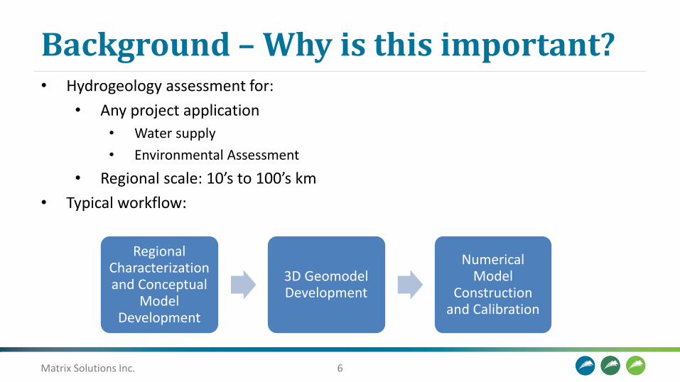
• Typical workflow:
Regional Characterization and Conceptual
Model Development
3D GeomodelDevelopment
Numerical Model
Construction and Calibration
Matrix Solutions Inc. 7
Background – Why is this important?
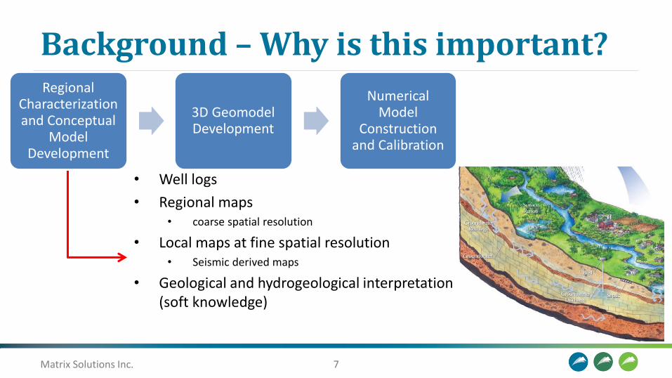
• Well logs
• Regional maps • coarse spatial resolution
• Local maps at fine spatial resolution• Seismic derived maps
• Geological and hydrogeological interpretation (soft knowledge)
Regional Characterization and Conceptual
Model Development
3D GeomodelDevelopment
Numerical Model
Construction and Calibration

Matrix Solutions Inc. 8
Background – Why is this important?
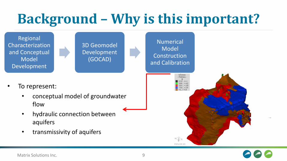
• To represent major hydrostratigraphic units into a 3D frame
• To consider different levels of confidence in the available data
• Interpolation of units structure can play an important role in numerical model of groundwater flow
Regional Characterization and Conceptual
Model Development
3D GeomodelDevelopment
Numerical Model
Construction and Calibration
Matrix Solutions Inc. 9
Background – Why is this important?
• To represent:
• conceptual model of groundwater flow
• hydraulic connection between aquifers
• transmissivity of aquifers
Regional Characterization and Conceptual
Model Development
3D Geomodel Development
(GOCAD)
Numerical Model
Construction and Calibration
Matrix Solutions Inc. 10
Cokriging

Matrix Solutions Inc. 11
Cokriging
• Kriging:– Learn from your initial data:
• To define the spatial structure for interpolation
–Apply optimal weights to your data points–Take into account:
• Distance between data points and points to interpolate• Structure of variable through:
– the trend– the variogram
Matrix Solutions Inc. 12
Cokriging
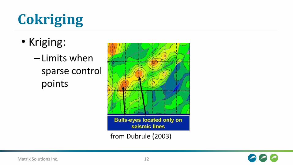
• Kriging:
– Limits when sparse control points
from Dubrule (2003)
Matrix Solutions Inc. 13
Cokriging
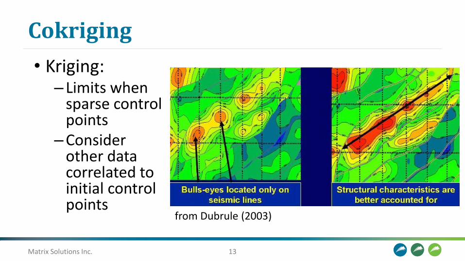
• Kriging:– Limits when
sparse control points
–Consider other data correlated to initial control points
from Dubrule (2003)

Matrix Solutions Inc. 14
Cokriging
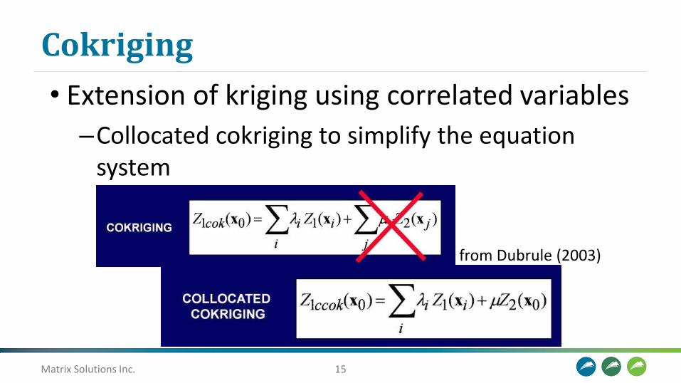
• Extension of kriging using correlated variables
from Dubrule (2003)• Z1 : primary data• Z2 : secondary data
Matrix Solutions Inc. 15
Cokriging
• Extension of kriging using correlated variables
–Collocated cokriging to simplify the equation system
from Dubrule (2003)
Matrix Solutions Inc. 16
Example 1 – Mapping a Structural Unconformity
Matrix Solutions Inc. 17
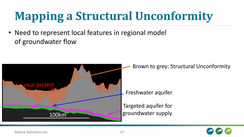
Mapping a Structural Unconformity• Need to represent local features in regional model
of groundwater flow
100km
Freshwater aquifer
Targeted aquifer forgroundwater supply
your project
Brown to grey: Structural Unconformity
Matrix Solutions Inc. 18
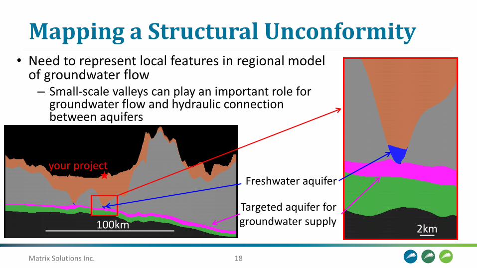
Mapping a Structural Unconformity• Need to represent local features in regional model
of groundwater flow– Small-scale valleys can play an important role for
groundwater flow and hydraulic connection between aquifers
100km
Freshwater aquifer
Targeted aquifer forgroundwater supply
2km
your project
Matrix Solutions Inc. 19
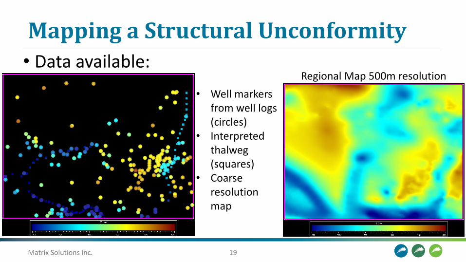
Mapping a Structural Unconformity
• Data available:Regional Map 500m resolution
• Well markers from well logs (circles)
• Interpreted thalweg(squares)
• Coarse resolution map
Matrix Solutions Inc. 20
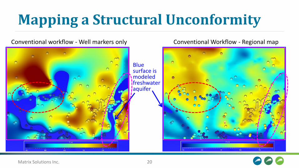
Mapping a Structural Unconformity
Conventional Workflow - Regional map only
Conventional workflow - Well markers only
Blue surface is modeled freshwater aquifer
Matrix Solutions Inc. 21
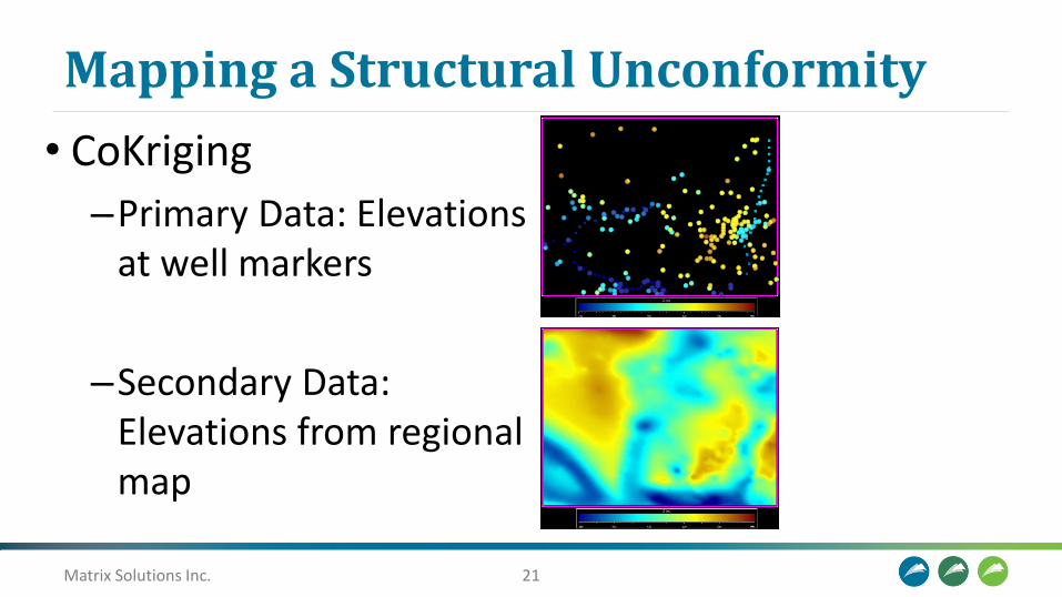
Mapping a Structural Unconformity
• CoKriging
–Primary Data: Elevations at well markers
–Secondary Data: Elevations from regional map
Matrix Solutions Inc. 22
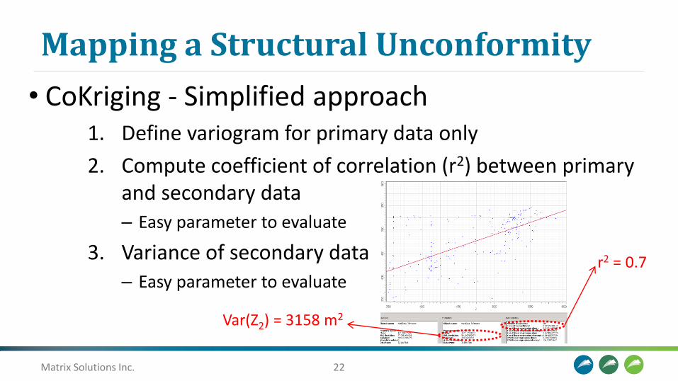
Mapping a Structural Unconformity
• CoKriging - Simplified approach1. Define variogram for primary data only
2. Compute coefficient of correlation (r2) between primary and secondary data– Easy parameter to evaluate
3. Variance of secondary data– Easy parameter to evaluate
r2 = 0.7
Var(Z2) = 3158 m2
Matrix Solutions Inc. 23
Mapping a Structural Unconformity
• CoKriging
–1st step: Define variogram on primary data:
• variation of variance with distance between data points
• Learn from the data to find best function for interpolation
Matrix Solutions Inc. 24
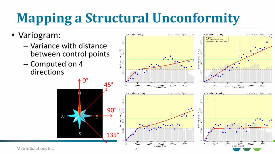
Mapping a Structural Unconformity• Variogram:
– Variance with distance between control points
– Computed on 4 directions
0°45°
90°
135°
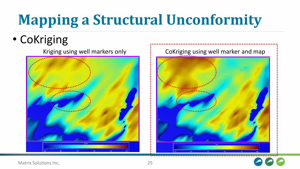
Matrix Solutions Inc. 25
Mapping a Structural Unconformity
Kriging using well markers only
• CoKrigingCoKriging using well marker and map
Matrix Solutions Inc. 26
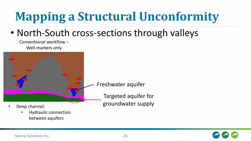
Mapping a Structural Unconformity• North-South cross-sections through valleys
Conventional workflow –Well markers only
Freshwater aquifer
Targeted aquifer forgroundwater supply
• Deep channel:• Hydraulic connection
between aquifers
Matrix Solutions Inc. 27
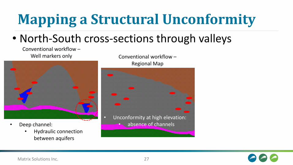
Mapping a Structural Unconformity• North-South cross-sections through valleys
Conventional workflow –Well markers only Conventional workflow –
Regional Map
• Deep channel:• Hydraulic connection
between aquifers
• Unconformity at high elevation:• absence of channels

Matrix Solutions Inc. 28
Mapping a Structural Unconformity• North-South cross-sections through valleys
CoKrigingConventional workflow –Well markers only Conventional workflow –
Regional Map
• Shallow channel:• No hydraulic
connection between aquifers
• Deep channel:• Hydraulic connection
between aquifers
• Unconformity at high elevation:• absence of channels
Matrix Solutions Inc. 29
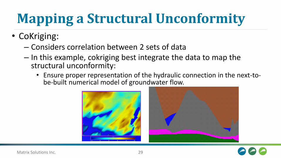
Mapping a Structural Unconformity• CoKriging:
– Considers correlation between 2 sets of data– In this example, cokriging best integrate the data to map the
structural unconformity:• Ensure proper representation of the hydraulic connection in the next-to-
be-built numerical model of groundwater flow.

Matrix Solutions Inc. 30
Example 2 – Mapping Net Isopach
Matrix Solutions Inc. 31
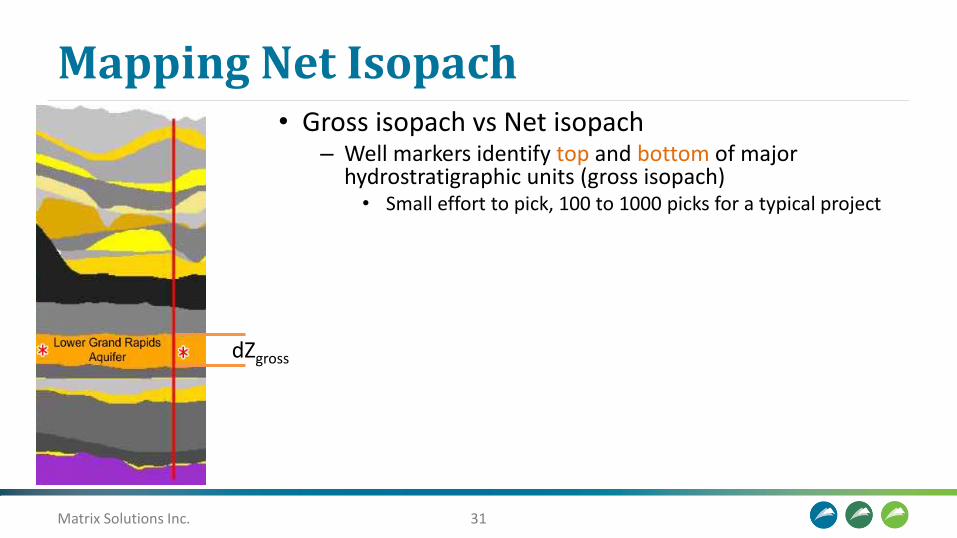
Mapping Net Isopach
dZgross
• Gross isopach vs Net isopach– Well markers identify top and bottom of major
hydrostratigraphic units (gross isopach)• Small effort to pick, 100 to 1000 picks for a typical project

Matrix Solutions Inc. 32
Mapping Net Isopach• Gross isopach vs Net isopach
– Well markers identify top and bottom of major hydrostratigraphic units (gross isopach)• Small effort to pick, 100 to 1000 picks for a typical project
– but if we look at the well logs within that unit
Matrix Solutions Inc. 33
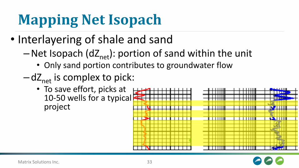
Mapping Net Isopach
• Interlayering of shale and sand–Net Isopach (dZnet): portion of sand within the unit
• Only sand portion contributes to groundwater flow
–dZnet is complex to pick:• To save effort, picks at
10-50 wells for a typical project
Matrix Solutions Inc. 34
Mapping Net Isopach
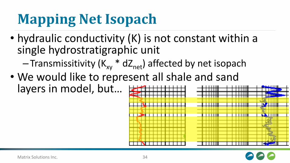
• hydraulic conductivity (K) is not constant within a single hydrostratigraphic unit–Transmissitivity (Kxy * dZnet) affected by net isopach
• We would like to represent all shale and sand layers in model, but…
Matrix Solutions Inc. 35
Mapping Net Isopach
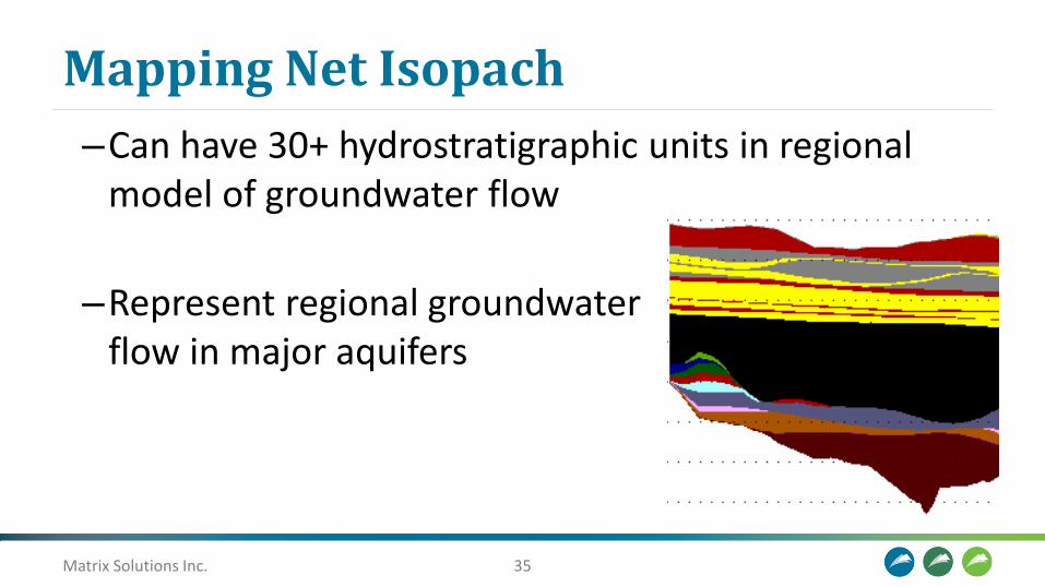
–Can have 30+ hydrostratigraphic units in regional model of groundwater flow
–Represent regional groundwater flow in major aquifers
Matrix Solutions Inc. 36
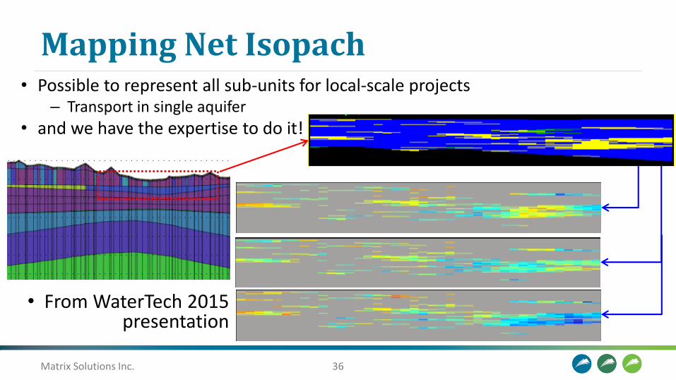
Mapping Net Isopach• Possible to represent all sub-units for local-scale projects
– Transport in single aquifer
• and we have the expertise to do it!
• From WaterTech 2015 presentation
Matrix Solutions Inc. 37
Mapping Net Isopach
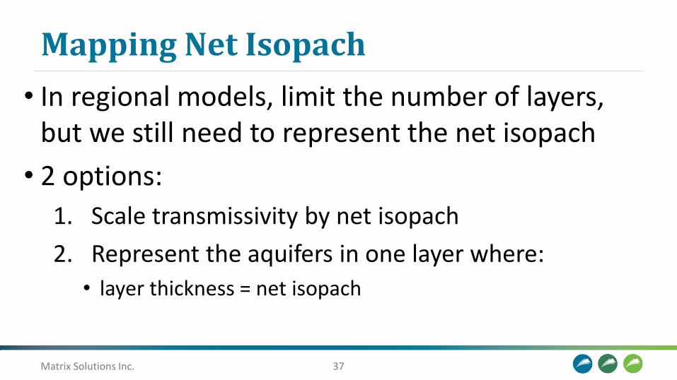
• In regional models, limit the number of layers, but we still need to represent the net isopach
• 2 options:
1. Scale transmissivity by net isopach
2. Represent the aquifers in one layer where:
• layer thickness = net isopach

Matrix Solutions Inc. 38
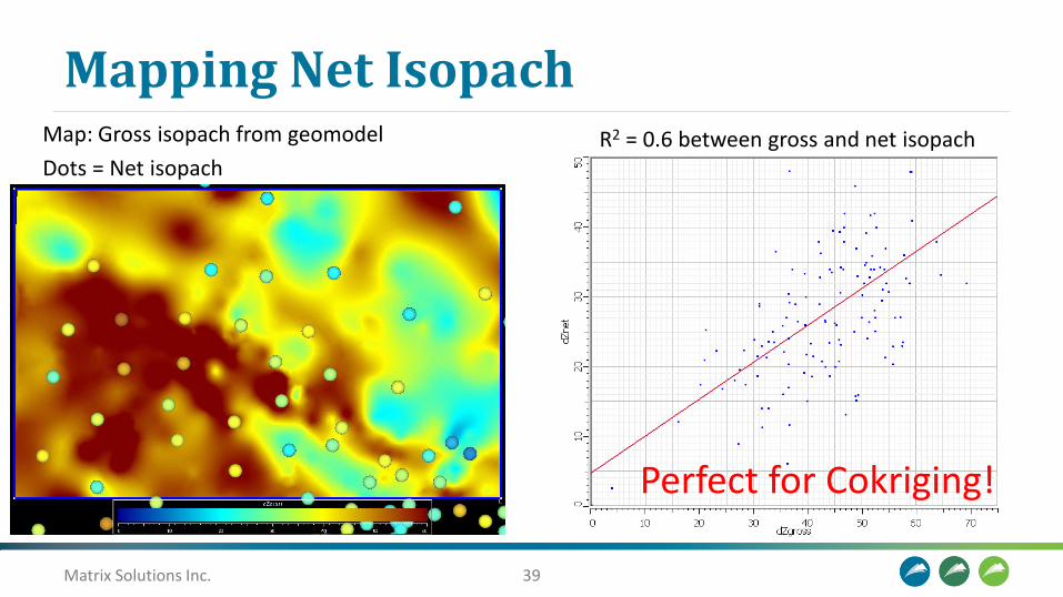
Mapping Net IsopachMap: Gross isopach from geomodel
Dots = Net isopach
0m (blue) to 60m (red)
Matrix Solutions Inc. 39
Mapping Net IsopachMap: Gross isopach from geomodel
Dots = Net isopachR2 = 0.6 between gross and net isopach
Perfect for Cokriging!
Matrix Solutions Inc. 40
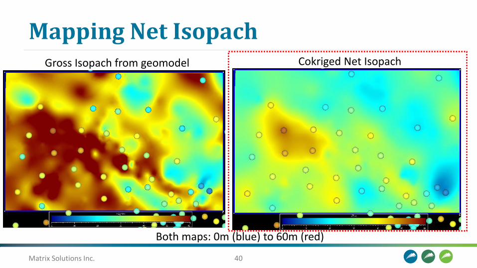
Mapping Net IsopachGross Isopach from geomodel Cokriged Net Isopach
Both maps: 0m (blue) to 60m (red)
Matrix Solutions Inc. 41
Mapping Net Isopach
• What impact does it have on regional groundwater flow?– Let’s assume the aquifer’s horizontal conductivity:
• Kxy = 5x10⁻⁵ m/s
–… and we compute the transmissivity (T) of the aquifer• T = K * dz
Matrix Solutions Inc. 42
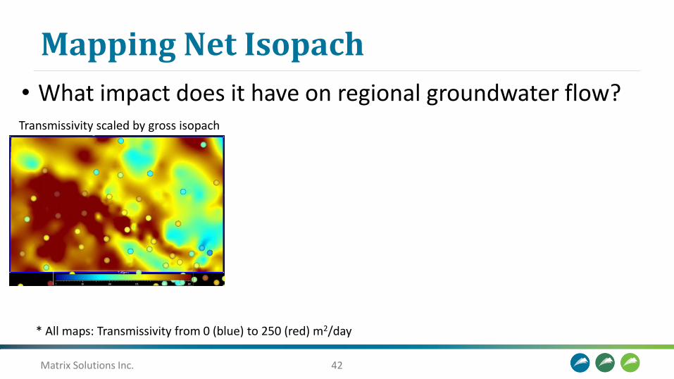
Mapping Net Isopach
• What impact does it have on regional groundwater flow?Transmissivity scaled by gross isopach
* All maps: Transmissivity from 0 (blue) to 250 (red) m2/day

Matrix Solutions Inc. 43
Mapping Net Isopach
• What impact does it have on regional groundwater flow?Transmissivity scaled by gross isopach
* All maps: Transmissivity from 0 (blue) to 250 (red) m2/day
Transmissivity scaled by net isopachinterpolated from well markers only
Matrix Solutions Inc. 44
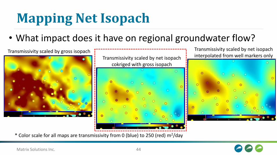
Mapping Net Isopach
• What impact does it have on regional groundwater flow?Transmissivity scaled by gross isopach
* Color scale for all maps are transmissivity from 0 (blue) to 250 (red) m2/day
Transmissivity scaled by net isopachcokriged with gross isopach
Transmissivity scaled by net isopachinterpolated from well markers only

Matrix Solutions Inc. 45
Conclusions
Matrix Solutions Inc. 46
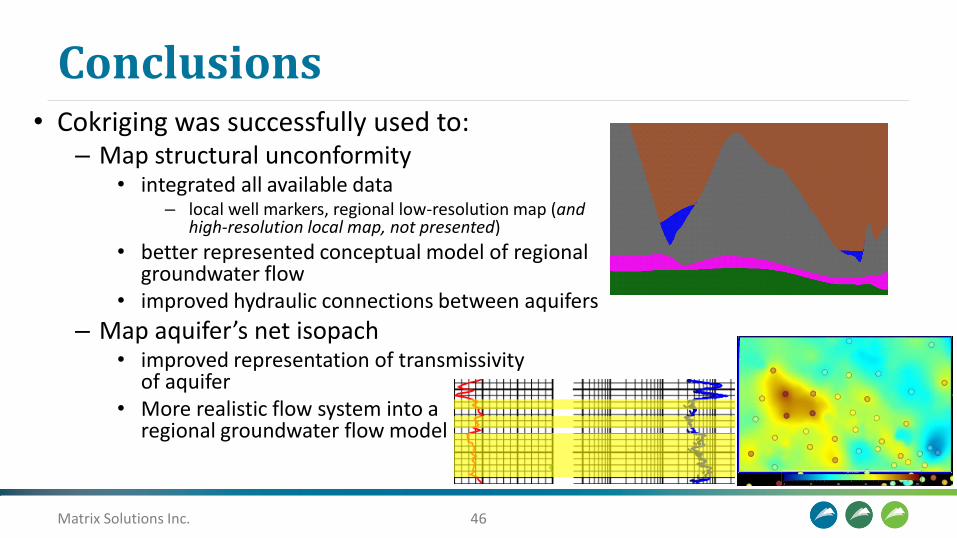
Conclusions• Cokriging was successfully used to:
– Map structural unconformity • integrated all available data
– local well markers, regional low-resolution map (and high-resolution local map, not presented)
• better represented conceptual model of regional groundwater flow
• improved hydraulic connections between aquifers
– Map aquifer’s net isopach• improved representation of transmissivity
of aquifer• More realistic flow system into a
regional groundwater flow model

Matrix Solutions Inc. 47
Matrix Contacts
• Maxime [email protected]
• Alexander [email protected]
• Louis-Charles [email protected]